


Abstract
Food manufacturing faces challenges in balancing efficiency, energy use, and quality. This paper presents a Hybrid Digital Twin Architecture (HDTA). It combines simulation, constraint programming, and Industrial IoT into a closed-loop system. The architecture has three layers: simulation for planning, optimization for scheduling, and an edge layer for control. We validated this using a bakery model with 10 products. The results show a 24.4% reduction in production time and 23% energy savings. Simulation results show complete elimination of quality time-window violations (0.0% vs. 13.3% baseline, p < 0.001). The system achieved a 2.4-month return on investment. This work demonstrates how combining these technologies can improve process industries.
1. Introduction
This work advances intelligent manufacturing by addressing the intersection of cybersecurity, energy optimization, and real-time control in Industry 4.0. The proposed Hybrid Digital Twin Architecture (HDTA) targets three challenges: (1) secure integration of distributed sensor networks into cyber-physical production systems; (2) minimization of energy costs under dynamic tariffs while preserving strict quality; and (3) edge deployment of computational intelligence to ensure deterministic low-latency control for time-sensitive batch processes. These challenges are especially acute in food manufacturing, characterized by biochemical constraints, energy-intensive thermal operations, and cybersecurity risks.
1.1. Research Context and Industrial Motivation
The global food manufacturing sector (≈$8.2 trillion/year) faces simultaneous pressures to improve efficiency, sustainability, and quality [1]. Bakery production is particularly challenging: it accounts for ≈12% of food-processing energy in developed economies and combines time-sensitive biochemical processes (fermentation, proofing), high energy intensity (60–70% in thermal operations), and complex multi-stage batch scheduling with hard temporal quality constraints [2].
Conventional planning (spreadsheets, FIFO, heuristics) leads to 15–20% spoilage due to time-window violations, 25–30% excess energy costs, and underutilized capacity [3], and it cannot handle the combinatorial complexity of multi-product, multi-machine scheduling under dynamic tariffs.
Industry 4.0 technologies—Digital Twins (DT), IIoT, and edge computing—enable virtual replicas of production systems with predictive analysis, prescriptive optimization, and autonomous control via real-time bidirectional data exchange [4]. Integrated with IIoT sensor networks, digital twins become cyber-physical systems (CPS) where algorithms directly control physical processes through deterministic feedback loops [5].
1.1.1. Rationale for Bakery Manufacturing as Application Domain
Biochemical time-sensitivity. Fermentation and proofing have strict temporal windows (typically ±15–30 min) defined by enzymatic activity, yeast metabolism, and gluten development [3]. Violations cause irreversible quality loss and batch disposal, making scheduling a quality-critical optimization problem where mathematical methods outperform simple heuristics.
Energy intensity and tariff response. Tunnel ovens (120–150 kW) account for 60–70% of bakery energy costs [2]. Differences of 40–60% between peak and off-peak tariffs offer annual savings of $50,000–$150,000 for medium-scale plants (1000–2000 units/day) via time-of-use-aware load shifting, providing strong economic motivation.
Structural representativeness. The multi-stage batch structure with precedence constraints, alternative machines, and quality time windows is typical for dairy, pharmaceuticals, beverages, and specialty chemicals, covering greater than $3 trillion/year of production value. Demonstrating HDTA in bakeries supports transferability to these sectors.
Small and medium bakeries with limited IT infrastructure are also ideal to demonstrate that advanced digital twin solutions can achieve fast payback (<6 months) without enterprise-scale resources, addressing a key barrier to Industry 4.0 adoption in SMEs.
This combination of hard temporal constraints (RQ1), energy intensity with tariff response (RQ1, RQ4), and edge computing requirements (RQ2) makes bakery manufacturing an ideal domain to validate the HDTA framework. The lessons learned are directly transferable to other process industries with similar characteristics (dairy, pharmaceuticals, beverages), as discussed in Section 4.5.
1.1.2. Research Gap Analysis
Despite extensive work on digital twins and CPS, three architectural gaps restrict autonomous manufacturing control:
Gap 1—Decoupled simulation and optimization. DES and optimization are usually separate tools linked by manual data transfer. DES provides detailed “what-if” analysis but no prescriptive schedules [6]; MILP/CP can compute optimal schedules but rely on static parameters that ignore real-world variability and degradation [7]. This decoupling produces schedules that degrade when implemented on the shop floor.
Gap 2—Cloud-centric architectures and latency. Cloud-based twins centralize computation [8] but introduce 100–500 ms network latency and variable response times [9], incompatible with time-critical food processes where minute-level deviations can cause batch loss. Industry requires deterministic control response <1 s, which cloud architectures cannot guarantee.
Gap 3—Lack of closed-loop calibration. Most twins operate in an open loop: model outputs are not systematically updated using execution data [10]. As equipment and materials evolve, accuracy degrades, requiring costly manual recalibration or full model rebuilding.
Research gap statement. No existing work demonstrates an architecture that simultaneously: (a) couples high-fidelity DES with mathematical optimization via automated bidirectional data exchange; (b) deploys optimization at the edge for deterministic low-latency control; and (c) implements systematic closed-loop calibration where execution data continuously refine simulation models. This is particularly critical in food batch manufacturing with strict quality windows and energy optimization requirements.
1.1.3. Research Questions
This study addresses four questions derived from these gaps:
RQ1 (Gap 1—Integration). Can bidirectional integration of DES and CP optimization significantly improve makespan, energy consumption, and quality compliance compared with heuristic scheduling and decoupled workflows?
RQ2 (Gap 2—Edge viability). Does edge deployment of CP-SAT provide (a) solution quality comparable to cloud/offline optimization, (b) solve times < 120 s for industrial-scale cases, and (c) efficiency sufficient for re-optimization every 2–4 h?
RQ3 (Gap 3—Closed-loop learning). Can automated calibration using IIoT data maintain digital twin accuracy (MAPE < 5%) for ≥180 days without manual intervention and detect/adapt to evolving system conditions?
RQ4 (Cross-cutting—Economics). Does HDTA achieve payback < 6 months when accounting for hardware, software, engineering costs and benefits in throughput, energy savings, and quality, thereby supporting SME adoption?
1.1.4. Research Hypotheses
Each research question is linked to a testable hypothesis with explicit targets:
H1.
Makespan reduction (RQ1).
H10.
μ_HDTA ≥ μ_FIFO (no makespan reduction).
H11.
μ_HDTA ≤ 0.80·μ_FIFO (≥20% reduction).
Test: paired t-test with Bonferroni correction (α = 0.05); target effect size d ≥ 0.8.
H2.
Edge performance (RQ2).
H20.
edge CP-SAT fails to achieve acceptable solve times.
H21.
mean solve time ≤ 120 s for 50 products × 6 operations on Raspberry Pi 4B (4 GB, quad-core ARM).
Method: computational experiments for 10–50 products, measuring solve time, optimality gap, and hardware utilization.
H3.
Energy–quality trade-off (RQ1).
H30.
TOU-aware energy optimization increases quality time-window violations.
H31.
energy cost reduction ≥ 15% with zero time-window violations (100% biochemical compliance).
Method: multi-objective analysis over 30 simulation replications.
H4.
Calibration accuracy (RQ3).
H40.
closed-loop calibration does not maintain model accuracy over extended operation.
H41.
weekly automated calibration maintains MAPE ≤ 5% for throughput, cycle time, and utilization over 180 days.
Method: longitudinal comparison of simulated and actual KPIs with weekly validation.
1.2. Research Contributions
The Hybrid Digital Twin Architecture (HDTA) closes these gaps through a three-layer framework combining predictive simulation, prescriptive optimization, and edge execution with continuous learning:
- Architectural innovation. First closed-loop integration of high-fidelity DES (Siemens Plant Simulation), CP optimization (OR-Tools CP-SAT), and edge computing (Raspberry Pi + 17 ESP32 IIoT nodes) with fully automated bidirectional data exchange, realizing a true digital twin per Kritzinger et al. [10].
- Methodological advancement. Edge deployment of CP-SAT for multi-objective batch scheduling that jointly minimizes makespan and energy cost under machine no-overlap, biochemical quality windows, and peak power constraints, achieving sub-second control and ~73 s solve times with 10–100× speedup over typical MILP.
- Cyber-physical realization. Integration of distributed IIoT sensing (environment, energy, weight) with edge intelligence to form a CPS where virtual models deterministically control manufacturing via sub-second feedback loops, secured by MQTT authentication, TLS, certificates, and network segmentation.
- Quantified industrial impact. Thirty simulation replications on a validated bakery model show 24.4% makespan reduction, 23.06% energy savings, zero quality violations, and payback in 2.4 months; TOU-aware scheduling shifts 67% of energy-intensive load to off-peak periods, enabling participation in demand response programs.
- Generalizability and scalability. A modular, technology-agnostic architecture with clear interfaces extends to dairy, pharmaceuticals, beverages, and chemicals; experiments for 10–50 products demonstrate sub-linear growth of solve time, supporting industrial-scale deployment.
Scope Definition and Research Boundaries
In scope:
Deterministic scheduling with known products, process parameters, and orders.
Multi-objective optimization of makespan and energy cost under dynamic TOU tariffs.
Hard biochemical quality constraints (fermentation/proofing time windows).
Edge-deployed optimization with IIoT-based monitoring and closed-loop calibration.
Cybersecurity for industrial CPS (authentication, encryption, segmentation).
Economic analysis (implementation costs, operational savings, ROI).
Outside scope (future work): *
Stochastic demand and probabilistic order arrivals.
Multi-site supply chain coordination.
Integrated preventive maintenance and reliability modeling.
Workforce scheduling and human-factor optimization.
Fully real-time quality control from in-line sensors (weight, temperature).
Machine learning for parameter tuning or dynamic objective weighting (α fixed at 0.15).
2. Related Work
2.1. Digital Twins in Manufacturing Systems
The digital twin concept has evolved into a foundational paradigm for Industry 4.0 [4, 11]. Tao et al. define it through three elements: physical system, virtual model, and bidirectional data connections [12]. While recent reviews highlight applications in maintenance and planning [13], Kritzinger et al. [10] distinguish true digital twins from lower-maturity variants. They classify systems as digital models (manual data) or digital shadows (unidirectional monitoring). A true digital twin requires automated bidirectional flow to control physical operations. Notably, 68% of industrial cases remain at the Shadow level, lacking the closed-loop control necessary for optimization [10]. Research in food sectors often focuses on specific domains. For instance, recent studies have applied digital twins to beverage bottling [14] and precision agriculture [15]. However, these works typically operate as open-loop systems or “digital shadows” geared towards monitoring, rather than the closed-loop prescriptive control required for complex batch scheduling.
2.2. Cyber-Physical Systems and Industrial IoT
Cyber-Physical Systems (CPS) converge computational algorithms with physical processes [5], often utilizing frameworks like the 5C architecture [16]. The Industrial Internet of Things (IIoT) supports this through edge computing, which is critical for real-time applications [9]. Shi et al. [9] emphasize that manufacturing IIoT requires deterministic latency (<100 ms), local processing, and fault tolerance. However, current research primarily targets predictive maintenance [17] or quality monitoring [18], rather than production control. While recent studies explore edge application placement [19] or reinforcement learning for scheduling [20], they often lack integration with discrete-event simulation. Consequently, deploying mathematical optimization solvers at the edge for closed-loop control remains a significant research gap.
2.3. Production Scheduling Optimization Methods
Job-shop scheduling is an NP-hard problem [21]. While Mixed-Integer Linear Programming (MILP) is the standard approach [7, 22], it struggles with discrete constraints and scales exponentially [23]. Constraint Programming (CP), particularly the CP-SAT solver, handles these logic-heavy problems more efficiently, achieving 10–100× speedups over MILP [24, 25]. However, CP applications in food manufacturing remain limited to single-objective or static problems [26], often missing the opportunity for multi-objective dynamic optimization.
2.4. Energy Optimization in Process Industries
Energy costs represent a major expense in industrial bakeries [2]. While Time-of-Use (TOU) tariffs offer opportunities for cost reduction [27], integrating them into production scheduling is complex. Previous studies have demonstrated cost savings using heuristics [28] or MILP [29]. However, these approaches often treat energy as a soft constraint or ignore the hard biochemical time windows required for food quality [3]. This work addresses these limitations by formulating energy limits and quality windows as hard constraints within a constraint programming framework.
2.5. Research Positioning
Table 1 positions our HDTA against existing approaches. Unlike methods that prioritize global optimality at the cost of speed (MILP) or connectivity without control (standard IoT), HDTA combines the speed of Constraint Programming with the closed-loop feedback of a digital twin.
Table 1.
Comparative analysis of digital twin and cyber-physical system approaches in manufacturing.
In summary, HDTA advances the state-of-the-art by transitioning optimization from cloud-based environments to the edge. This shift enables deterministic, closed-loop control that maintains strict quality constraints—a capability that traditional offline or open-loop methodologies often fail to guarantee.
3. Proposed Hybrid Digital Twin Architecture
3.1. System Architecture Overview
The Hybrid Digital Twin Architecture (HDTA) establishes a hierarchical, closed-loop cyber-physical system designed to bridge the gap between predictive simulation and deterministic control. As illustrated in Figure 1, the HDTA operates through a sequential data pipeline that transitions from high-level stochastic simulation to deterministic edge execution. The workflow relies on file-based integration, where the structural constraints defined in the Predictive Modeling layer (Fixed.json) serve as the requisite input for the Prescriptive Optimization engine to generate an actionable timeline (Schedule.json). Crucially, the architecture distinguishes itself through the feedback loop depicted by the ascending red trajectory; this mechanism aggregates real-world performance data (Actual.json) from the physical IIoT nodes and cycles it back to the digital twin. Consequently, this closed-loop design enables continuous calibration of the simulation parameters, ensuring that the predictive model dynamically adapts to the evolving reality of the shop floor.
Figure 1.
Schematic representation of the Hybrid Digital Twin Architecture (HDTA). The framework is organized into three hierarchical levels: Layer 1 (Predictive Modeling) utilizes Siemens Plant Simulation for stochastic parameter definition; Layer 2 (Prescriptive Optimization) employs Google OR-Tools CP-SAT for constraint satisfaction and scheduling; and Layer 3 (Edge Execution and IIoT) manages physical deployment via Raspberry Pi and ESP32 nodes. The red arrow denotes the closed-loop calibration mechanism, wherein historical telemetry data (Actual.json) is reintroduced into the simulation layer to refine predictive accuracy.
The architecture operates through three hierarchical layers (see Figure 1):
Layer 1: Predictive Modeling. Uses Siemens Plant Simulation to analyze historical data and identify bottlenecks. It generates the structural constraints and parameters (Output: Fixed.json). While Layer 2 generates the optimal schedule, Layer 1 (DES) serves a critical dual purpose. First, it acts as a ‘digital sandbox’ to validate the feasibility of the CP-SAT schedule under stochastic conditions (e.g., machine breakdowns) before physical execution. Second, it aggregates raw, noisy IIoT data into reliable statistical distributions required by the solver, bridging the gap between physical uncertainty and deterministic optimization.
Layer 2: Prescriptive Optimization. The decision engine uses Google OR-Tools CP-SAT. It calculates optimal schedules by balancing production speed against energy costs under TOU tariffs (Output: Schedule.json).
Layer 3: Edge Execution. A Raspberry Pi gateway orchestrates 17 distributed IIoT nodes. It guarantees deterministic control, monitors execution, and sends data back to Layer 1 for calibration (Output: Actual.json).
Architectural Design Principles:
The HDTA design embodies four fundamental principles essential for cyber-physical system realization:
- Separation of Concerns with Defined Interfaces. Predictive modeling (Layer 1), prescriptive optimization (Layer 2), and execution control (Layer 3) are architecturally decoupled with well-defined data contracts (Fixed.json, Schedule.json, Actual.json). This modularity enables independent development, testing, modification, and scaling of each layer without system-wide disruption, facilitating incremental industrial adoption and technology substitution.
- Data-Driven Automated Integration. Layers communicate through standardized JSON-formatted data contracts transmitted via file system (Layers 1↔2) and MQTT messaging (Layers 2↔3). This eliminates manual data transcription errors, enables automated workflow orchestration, and facilitates integration with existing Enterprise Resource Planning (ERP) and Manufacturing Execution Systems (MESs) through standard APIs.
- Continuous Closed-Loop Calibration. Actual execution data from Layer 3 automatically flows back to Layer 1 through weekly InfluxDB exports, enabling continuous model refinement without manual intervention. Statistical analysis identifies parameter drift, triggering automated distribution updates and bottleneck re-analysis. This closed-loop feedback transforms the digital twin from a static model to an adaptive, self-improving cyber-physical system.
- Edge-Centric Deterministic Control. Critical control path (optimization → execution → monitoring) operates entirely at the edge computing layer, guaranteeing sub-second response times independent of internet connectivity, cloud availability, or network congestion. This deterministic latency is essential for time-critical food manufacturing processes where biochemical reactions continue regardless of computational delays.
3.2. Layer 1: Discrete-Event Simulation Digital Twin
3.2.1. Production System Modeling Framework
The physical bakery production system was modeled using Siemens Plant Simulation v16.2, a commercial discrete-event simulation environment widely adopted in manufacturing engineering and validated through extensive industrial deployment [30]. The model represents a medium-scale bakery facility processing multiple product families with varying process requirements, quality constraints, and energy consumption profiles.
Production Line Configuration:
The modeled six-stage production line mirrors typical industrial bakery layouts:
- Mixing Station: Two parallel planetary mixers (50 kg batch capacity, 15 kW motor power) processing 10 recipe variants with product-specific ingredient formulations (flour types, hydration levels, yeast concentrations) and mixing durations
- Resting Chambers: Four temperature-controlled fermentation chambers (ambient to 25 °C, capacity 8 batches each) for biochemical fermentation initiation and gluten development
- Forming Station: Two parallel sheeting/molding machines (12–18 kW power) for dough shaping, portioning, and panning operations
- Proofing Chambers: Three humidity/temperature-controlled proofing cabinets (30–35 °C, 75–85% relative humidity, 1.5 kW heating/humidification) for final fermentation and volume development—identified through bottleneck analysis as primary capacity constraint
- Baking Tunnel Oven: Single continuous gas-fired tunnel oven. In this study, it is modeled as the dominant energy consumer with three distinct operational states:
- •
- Baking: High load (~140 kW) during active processing;
- •
- Idle: Medium load (~80 kW) to maintain thermal equilibrium during short gaps between batches;
- •
- Cold Start: A significant energy and time penalty required to ramp up from ambient temperature if the oven is shut down.
The optimization objective is to minimize ‘Idle’ duration and eliminate ‘Cold Starts’ by clustering baking tasks (campaigning), which prevents the energy waste typical of fragmented production schedules.
- 6.
- Cooling and Packaging: 2 parallel cooling conveyors with forced air circulation (8.5 kW fans) followed by automated packaging lines for product inspection, wrapping, and case packing
Material Flow Logic and Routing: Raw materials (flour, water, yeast, salt, sugar, fats, functional additives) enter the mixing stage where product-specific recipes determine ingredient proportions, mixing speeds (60–120 rpm), and mixing durations. Semi-finished dough progresses through resting for fermentation initiation (enzymatic activity, gas production), forming for shaping and weight portioning, and proofing for final volume development before entering the baking oven. Finished products undergo forced-air cooling to ambient temperature, quality inspection (visual, weight verification), and automated packaging. Inter-stage material transport is modeled with realistic conveyor speeds (0.3–0.5 m/s) and product-dependent changeover times (3–8 min for cleaning/sanitization when switching between product families).
3.2.2. Stochastic Process Characterization
Processing time uncertainty was characterized using triangular probability distributions T [min, mode, max], selected for their ability to represent bounded variability with limited data while capturing realistic operational fluctuations [31]. Distribution parameters were calibrated from historical production data spanning 180 operational days (43,200 batches processed) collected from an industrial bakery facility through automated Manufacturing Execution System (MES) data logging (Table 2).
Table 2.
Calibrated stochastic processing time distributions and energy consumption profiles (time parameters in minutes; energy in kWh per batch; power in kW average; sample sizes: n = 150 for Mixing, n = 180 for Proofing, n = 90 for Baking, n = 75 for Cooling).
3.2.3. Bottleneck Analysis and Constraint Generation
The BottleneckAnalyzer module (custom SimTalk scripting) performs systematic capacity constraint identification through continuous monitoring of equipment utilization, upstream queue lengths, and work-in-process waiting times across all simulation replications, applying Theory of Constraints principles [32].
The bottleneck analysis yielded the following results. The primary bottleneck identified is the proofing stage: proofing chambers exhibited the highest utilization (94.7% ± 1.8%) and longest upstream queues (mean 2.3 ± 0.6 batches waiting, maximum observed 5 batches during demand peaks). Sensitivity analysis with ±20% capacity variations confirmed that proofing capacity directly constrains system throughput: a 10% increase in proofing capacity increases system throughput by 8.2%, shifting the bottleneck to the baking oven.
Secondary Bottleneck: Baking oven utilization (87.3%) is below the theoretical bottleneck threshold but represents a single point of failure with the highest energy intensity. Observed oven downtime (1.85%) disproportionately impacts system performance due to lack of parallel capacity and perishable upstream work-in-process.
Quality Time Window Constraints: Proofing operations impose hard temporal constraints derived from fermentation biochemistry. Insufficient proofing time yields dense products with underdeveloped gluten structure and poor volume; excessive proofing causes over-fermentation, carbon dioxide loss, gluten network collapse, and product failure [33]. These constraints are product-specific:
- •
- White Bread: [45, 75] minutes (tolerance window: 30 min)
- •
- Whole Wheat: [50, 80] minutes (tolerance: 30 min)
- •
- Croissant: [90, 150] minutes (tolerance: 60 min)
- •
- Baguette: [40, 60] minutes (tolerance: 20 min)
- •
- Pain de Mie: [55, 85] minutes (tolerance: 30 min)
3.3. Layer 2: Constraint Programming Optimization
3.3.1. Mathematical Problem Formulation
The production scheduling problem is formulated as a multi-objective flexible job-shop scheduling problem (FJSSP) with temporal quality constraints and dynamic energy pricing—an NP-hard combinatorial optimization challenge [21].
Before presenting the formal mathematical model, we provide an intuitive description of the problem. We solve a scheduling problem to minimize total production time and energy costs. The goal is to assign baking tasks to ovens when electricity is cheap, without delaying them so long that the dough spoils. The model respects three main rules: (1) a machine can only do one task at a time, (2) dough must be baked within a specific time window after mixing (quality constraint), and (3) total power usage must not exceed the factory limit.
- •
- Sets and Indices
I = {1, …, n\}: Set of products (jobs).
Ji = {1, …, mi}: Ordered set of operations for product i.
M = {1, …, K}: Set of available machines.
T = {0, …, H}: Discrete time horizon (minutes), where H = 1440 (24 h cycle).
- Parameters:
- •
- di,j: Nominal processing duration of operation j of job i (minutes).
- •
- , : Minimum and maximum allowed waiting times after operation (i,j) for quality assurance (minutes).
- •
- Mi,j ⊆ M: Set of eligible machines for operation (i,j).
- •
- Pi,j: Average power consumption (kW) of operation (i,j). Derived from total energy Ei,j as Pi,j = 60 Ei,j/di,j.
- •
- (t): Electricity tariff at time t ($/kWh). Off-peak: $0.12 (00:00–08:00, 20:00–24:00). Peak: $0.18 (08:00–20:00).
- •
- Plimit: Facility peak power demand limit (180 kW).
- •
- TEC*: Normalization factors for makespan and energy cost (e.g., theoretical lower bounds).
- Decision Variables:
- •
- Si,j ∈ [0, H]: Start time of operation (i,j).
- •
- Ci,j ∈ [0, H]: Completion time of operation (i,j).
- •
- xijk ∈ [0, H]: Binary variable, equal to 1 if operation (i,j) is assigned to machine k.
- •
- yijt ∈ [0, H]: Binary variable, equal to 1 if operation (i,j) is active at time t.
- •
- Objective Function: The objective is to minimize the weighted sum of the normalized makespan (Cmax) and total energy cost (TEC). The weight = 0.15 reflects the operational priority of meeting deadlines while opportunistically reducing energy costs.
The normalization constants and TEC* are determined based on the theoretical lower bounds of the system. is calculated as the sum of processing times of all jobs on the bottleneck resource (the Oven), representing the minimum possible makespan. TEC* is the theoretical minimum energy consumption required to process all batches, excluding any idle or warm-up energy penalties. These constants ensure that both objectives (time and energy) are scaled to a similar range [0, 1] before being weighted by and , where the makespan and total energy cost are defined as:
Constraint C6 prevents the trivial solution where energy cost is minimized by omitting jobs entirely. It guarantees that every product i ∈ I completes its final operation within the 24 h planning horizon H = 1440 min.
Weight α = 0.15 reflects operational priority: meeting production deadlines while opportunistically reducing energy costs. Normalization ensures comparable objective scales.
The selection of α = 0.15 in the objective function (Equation (1)) is predicated on the prior normalization of the makespan () and total energy cost (TEC) terms by their respective theoretical lower bounds1. Because the objective components are dimensionless, α functions strictly as a relative priority coefficient rather than a unit conversion factor. This scalarization implies a marginal rate of substitution of approximately 1:6.67; theoretically, the optimization solver is permitted to degrade the makespan by 1\% only if it yields a simultaneous reduction in energy costs of greater than 6.7\% (1/0.15). This configuration enforces a steep penalty on critical path extensions, constraining the solution space to the “knee” of the Pareto front. Consequently, the solver is mathematically coerced to seek “low-hanging fruit”—specifically, opportunistic temporal load shifting (e.g., delaying an oven start time) that exploits existing slack time to align with off-peak tariffs without expanding the global makespan. This ensures that energy optimization remains strictly ancillary to production throughput.
The model enforces the following hard constraints:
(C1) Precedence: Operations must follow technological sequence
(C2) Duration: Operation durations match DES parameters
(C3) Machine No-Overlap: Each machine can process at most one operation at any given time t
(C4) Quality Time Windows: Critical operations (e.g., proofing) must respect min/max bounds
(C5) Peak Energy Limit: Total instantaneous power draw cannot exceed facility capacity
(C6) Job Completion: All jobs must be scheduled and completed within the planning horizon
3.3.2. CP-SAT Solver Implementation and Configuration
The implementation utilizes the Google OR-Tools CP-SAT solver (v9.7), employing lazy clause generation, conflict-driven learning, and parallel portfolio search [11]. The solver is deployed on the Raspberry Pi 4B edge gateway and configured for industrial real-time constraints. Key parameters include a maximum solution time of 300 s (selected to balance solution quality with operational responsiveness for shift-level rescheduling), 8 parallel search workers (matching the Raspberry Pi 4B’s CPU core count), and an optimality tolerance of 0.1% relative gap using an automatic portfolio search strategy. For real-time rescheduling in response to minor floor disruptions, the solver typically terminates early upon finding high-quality solutions (mean 73.2 s for baseline instances), as demonstrated in Section 3.6.6. Computational Performance: For the baseline problem instance (n = 10 products, average mi = 6 operations, K = 11 machines, H = 1440 min), the edge-deployed solver demonstrates consistent performance suitable for operational control: Mean solution time: 73.2 s ( = 18.4 s). Solution Quality: Mean optimality gap of 0.08% at termination, with 76.7% of instances proven optimal. Resource Efficiency: CPU utilization averages 78%, ensuring sufficient capacity for concurrent IIoT processing, while RAM usage remains at 1.2 GB (leaving significant headroom on the 4 GB hardware). The solver outputs a Schedule.json file containing the optimized assignments.
3.4. Layer 3: Edge Computing and IIoT Infrastructure
3.4.1. Hardware Architecture
The physical layer comprises a network of 17 distributed IIoT sensor nodes based on ESP32-WROOM-32 microcontrollers (Dual-core 240 MHz, WiFi 802.11n, Espressif Systems, Shanghai, China.). These nodes interface with a suite of sensors via I2C, SPI, and ADC protocols to monitor critical process variables. The central orchestration is performed by a Raspberry Pi 4B Edge Gateway (Cambridge, UK). running a Dockerized stack containing the Mosquitto MQTT broker (v2.0.15), InfluxDB (v2.7) for time-series data, and Node-RED (v3.0.2) for control logic. Detailed specifications of the hardware components are provided in Table 3.
Table 3.
Hardware configuration of the edge gateway and distributed IIoT sensor nodes.
3.4.2. Communication Protocol and Security
To ensure the integrity of the closed-loop control system, a defense-in-depth security strategy was integrated directly into the communication architecture. The specifications of the inter-layer data exchange protocols are summarized in Table 4. Since the digital twin relies on trusted telemetry (Actual.json) for automated model calibration, protecting the feedback loop from data injection attacks is critical. The implementation employs strict Network Segmentation, isolating production VLANs from enterprise networks to prevent lateral movement. Data integrity is guaranteed via TLS 1.3 encryption for all MQTT traffic and mutual certificate-based authentication (mTLS) for edge nodes. Additionally, the edge gateway utilizes Fail2ban for intrusion detection and iptables to restrict traffic solely to authorized command and telemetry ports, ensuring that the prescriptive control commands sent to the shop floor cannot be intercepted or manipulated.
3.4.3. Closed-Loop Calibration
To maintain model fidelity over time, a weekly automated calibration procedure is implemented (see Figure 2). The workflow begins with extracting actual execution durations for the past 7 days from InfluxDB. Triangular distributions are fitted to this data using the method of moments (for samples n 30). A Kolmogorov–Smirnov test ( = 0.05) detects statistically significant parameter shifts. If a shift is detected, the Fixed.json contract is updated, and the Discrete-Event Simulation (DES) is re-run (10 replications) to validate the new parameters. Finally, bottleneck analysis is repeated; if resource utilization shifts by more than 5%, optimization constraints are regenerated.
Figure 2.
The closed-loop calibration cycle. The workflow proceeds clockwise from data extraction to validation. The Model Update phase (highlighted in red) is triggered conditionally based on the results of the Kolmogorov–Smirnov (KS) test (p < 0.05), ensuring that the Fixed.json simulation parameters are only revised when statistically significant deviations occur in the physical system.
As illustrated in Figure 2, the maintenance of digital twin fidelity is governed by an iterative, automated calibration loop designed to detect temporal drifts in process parameters. The cycle transitions from empirical data extraction to statistical validation, utilizing a Kolmogorov–Smirnov test to rigorously identify significant shifts in execution behavior before authorizing any modification to the core simulation parameters. Crucially, the process enforces a validation step where the updated model undergoes ten replication runs of the Discrete-Event Simulation (DES), ensuring that any adjustments to the Fixed.json contract effectively capture real-world phenomena such as equipment degradation or seasonal variances without introducing instability.
The calibration workflow is fully automated and executes weekly on Sunday at 02:00 (off-peak period to minimize computational interference with production). The entire process—from data extraction to constraint regeneration—completes in approximately 15–20 min without human intervention. Manual override is available via the Node-RED dashboard for emergency recalibration in response to significant equipment changes (e.g., oven replacement).
Table 4.
Inter-layer data exchange specifications.
3.5. Experimental Design
3.5.1. Industrial Context and Product Portfolio
The Hybrid Digital Twin Architecture (HDTA) was evaluated using a realistic case study of a medium-scale industrial bakery operating in a continuous 24 h production regime. The facility processes 10 product variants grouped into four families—white breads, whole grain breads, artisan products, and viennoiserie—representing a typical diversified product mix in industrial bakery operations [2,3,33].
Daily production volume in the simulated reference scenario corresponds to approximately 6700–8500 units per day, depending on demand variability and scheduling policy, which is consistent with energy benchmarks for medium bakeries (≈372 MWh/year, i.e., ≈1000–1100 kWh/day) [2,3]. Product-specific daily demand and batch sizes are summarized in Table 5.
Table 5.
Product portfolio and daily demand for the industrial bakery case study.
The physical production system follows the six-stage structure described in Section 3: two planetary mixers, four resting chambers, two forming machines, three proofing cabinets, a single tunnel oven, and two cooling/packaging lines. Proofing and baking stages constitute biochemical and thermal bottlenecks, respectively, and dominate both quality and energy performance [2,33].
3.5.2. Process Times and Quality Constraints
Unit process times for mixing, resting, forming, proofing, baking, and cooling were parameterized using triangular distributions calibrated from 180 days of historical data and cross-checked against bakery technology literature [30,31,33]. Table 6 summarizes representative ranges for a subset of products.
Table 6.
Representative processing time ranges (minutes) for key operations (triangular distributions T [min, mode, max]).
For proofing operations, quality-critical time windows were imposed as hard constraints in the optimization model, with minimum, optimal, and maximum residence times derived from fermentation kinetics [33]. For example, white bread requires proofing within [45, 75] min, while croissants require [90, 150] min; exceeding these windows leads to dense texture, loss of layering, or collapsed structure. These windows enforce a strict coupling between scheduling and quality.
3.5.3. Equipment and Energy Model
Equipment power ratings and energy consumption per batch are based on industrial audits of commercial bakeries [2,3]. Table 7 summarizes the main equipment considered in the energy model.
Table 7.
Equipment power ratings and typical energy consumption per batch.
Consistent with industrial studies, the tunnel oven accounts for 60–70% of total electrical energy consumption, while other stages contribute smaller but non-negligible shares [2,3]. Instantaneous power constraints and per-operation energy consumption values are passed to the CP-SAT model through the Fixed.json contract (Section 3.2).
3.5.4. Time-of-Use Tariff Structure
To capture economic incentives for demand-side management, the case study adopts a two-level Time-of-Use (TOU) tariff structure representative of industrial contracts:
- •
- Off-peak: 00:00–06:00 and 20:00–24:00, rate = 0.12 $/kWh
- •
- Mid-peak: 06:00–08:00 and 20:00–22:00, rate = 0.15 $/kWh
- •
- Peak: 08:00–20:00, rate = 0.18 $/kWh
Peak rates are approximately 50% higher than off-peak rates, consistent with demand-response literature [26,27,28]. The CP-SAT model minimizes a weighted sum of makespan and daily energy cost, subject to a hard peak power limit of 180 kW and quality time-window constraints, as defined in Section 3.3.
3.5.5. Experimental Scenarios
Two main scenarios were evaluated:
- •
- Baseline FIFO scheduling (Scenario S0).
- •
- First-In-First-Out (FIFO) dispatching of batches at each stage.
- •
- Round-robin assignment to parallel machines.
- •
- No consideration of TOU tariffs or energy limits beyond nominal capacity.
- •
- Quality is monitored ex-post; proofing time violations are not prevented proactively.
- •
- HDTA-optimized closed-loop scheduling (Scenario S1).
- •
- Layer-1 DES generates calibrated Fixed.json parameters and bottleneck information.
- •
- Layer-2 CP-SAT solves the multi-objective flexible job-shop scheduling problem with energy and quality constraints (weight α = 0.15).
- •
- Layer-3 edge execution enforces Schedule.json, monitors deviations, and logs actual execution data.
- •
- Weekly closed-loop calibration updates processing-time distributions and constraints.
Each scenario was simulated for 30 independent replications with different random seeds, using a 2 h warm-up period followed by a 24 h production run. This design enables rigorous statistical comparison between S0 and S1.
3.5.6. Statistical Analysis Protocol
For each replication, the following Key Performance Indicators (KPIs) were recorded:
Makespan (h) of the 24 h production plan.
- •
- Total electrical energy consumption (kWh).
- •
- Daily energy cost ($/day) under the TOU tariff.
- •
- Throughput (units/day of finished products).
- •
- Equipment uptime (% of scheduled time).
- •
- Quality time-window violations (% of batches outside proofing windows).
Paired two-sample t-tests were conducted between S0 and S1 for each KPI with Bonferroni-corrected significance level α = 0.05/8 = 0.00625. Effect sizes were quantified using Cohen’s d. Normality of paired differences was verified using Shapiro–Wilk tests (all p > 0.05).
Regarding data provenance and validation strategy, this study explicitly delineates between empirical input parameters and projected operational outcomes. The simulation model is grounded in physical reality: stochastic processing times were calibrated using 180 days (June–November 2024) of automated Manufacturing Execution System (MES) timestamp logs capturing actual start/completion times for 43,200 batches. Energy consumption profiles were derived from 60-day facility audits using portable power analyzers (Fluke 435-II (Fluke Corporation, Everett, USA.)) installed on each equipment group. Biochemical quality constraints were established through consultation with production engineers and validated against laboratory fermentation kinetics data from 150 batches subjected to deliberate time window variations [33].
3.6. Results
3.6.1. Primary Operational Performance
These results demonstrate statistically significant improvements across all KPIs with large effect sizes (Cohen’s d > 2.5), indicating strong practical significance. The 24.4% makespan reduction (H1) exceeds the targeted 20% threshold, confirming that bidirectional DES-CP integration substantially outperforms heuristic scheduling. The simultaneous 23.06% energy reduction with zero quality violations (H3) refutes the common assumption that energy optimization requires quality trade-offs; instead, the results show that tariff-aware scheduling enhances process synchronization, improving both efficiency and quality. Equipment uptime gains (+1.82 pp) reflect reduced idle time and better resource coordination. All p-values remain significant after Bonferroni correction (α = 0.00625), providing strong statistical evidence to reject the null hypotheses H10 and H30.
3.6.2. Temporal Load Shifting and Energy Cost Analysis
The projected annual savings of $69,335 are fundamentally driven by the solver’s ability to execute precise tariff arbitrage involving the facility’s dominant energetic load. By identifying that the Tunnel Oven (140 kW) accounts for the majority of instantaneous power draw, the CP-SAT algorithm strategically orchestrates dense production campaigns within the off-peak pricing windows ($0.12/kWh), thereby avoiding the prohibitive $0.18/kWh peak tariff. This 67% load shifting capability is operationally complex; it relies on the solver’s resolution of strict disjunctive constraints to synchronize the Proofing bottleneck with oven availability. The optimization engine effectively aligns the fermentation kinetics of the dough with the utility grid’s pricing structure, ensuring that semi-finished products are ready for baking exactly during low-cost energy intervals without violating the hard temporal windows required to prevent spoilage.
To understand how HDTA achieves lower energy costs, Figure 3 and Table 8 analyze temporal energy usage under TOU tariffs.
Figure 3.
Analysis of energy efficiency under Time-of-Use (TOU) tariffs. (A) Profile of instantaneous power demand (kW) over a 24 h cycle. The HDTA schedule (green trace) exhibits reduced volatility and lower peak demand compared to the FIFO baseline (red trace), particularly during the high-tariff window (08:00–20:00, highlighted in orange). (B) Cumulative energy consumption (kWh). The divergence between the two curves highlights a total energy saving of 560 kWh (23.1%) achieved by the proposed architecture.
Figure 3 provides a quantitative evaluation of the economic impact of the proposed architecture. As evidenced by the power demand profiles in Figure 3A, the HDTA system successfully leverages the flexibility of the job-shop environment to shift energy-intensive loads—specifically baking operations—away from the peak tariff window (08:00–20:00). This strategic load shifting is quantified in Figure 3B, where the cumulative energy consumption of the HDTA schedule is shown to be 23.1% lower than the FIFO baseline, demonstrating the efficacy of the constraint-based solver in minimizing operational costs without compromising throughput.
The representative day in Table 9 shows that HDTA reduces peak-period consumption by 1280 kWh (from 2180 to 900 kWh), representing a 58.7% reduction in peak demand. This is achieved through a combination of efficiency gains and shifting operations to off-peak and mid-peak windows. While total energy consumption decreases, the distribution shifts; HDTA utilizes proportionally more off-peak and mid-peak capacity relative to its total load, effectively leveraging the tariff differential. The net effect is a double benefit: (i) lower overall consumption (Table 8) and (ii) reduced exposure to peak tariffs. This supports the tariff-aware nature of HDTA and illustrates how energy savings consist of both physical reduction and tariff optimization.
Table 8.
Primary performance metrics for FIFO baseline (S0) and HDTA-optimized scheduling (S1) (mean ± SD, n = 30).
Table 9.
Representative daily energy distribution by TOU period for FIFO and HDTA schedules (values represent mean across 30 simulation replications).
3.6.3. Production Schedule Structure and Gantt-Level Insights
To further elucidate the operational mechanics behind the energy savings, Figure 4 contrasts the temporal distribution of baking tasks between the two scheduling strategies. It can be observed that the FIFO heuristic schedules batches reactively, leading to fragmented oven usage that frequently intersects with the expensive peak tariff window. In contrast, the HDTA optimizer enforces a “campaign-based” logic; as shown in the bottom timeline, it densely clusters production into the early morning off-peak sector and consolidates the remaining workload in the late afternoon. This reduces the frequency of oven warm-up phases and maximizes the volume of product processed during low-cost energy intervals.
Figure 4.
Comparative Gantt charts illustrating oven utilization for a representative subset of white bread batches. The shaded region denotes the peak tariff period (08:00–20:00). While the FIFO approach (top) results in sporadic oven usage distributed throughout the high-cost window, the HDTA schedule (bottom) aggregates baking tasks into dense, contiguous campaigns. This consolidation prioritizes the off-peak hours (02:00–06:00) and groups remaining necessary tasks, effectively minimizing idle time and thermal cycling.
The HDTA schedule exhibits tighter packing of oven batches, shorter idle gaps, and deliberate avoidance of high-tariff intervals. In contrast, FIFO scheduling generates fragmented oven utilization with extended idle periods and frequent “holes” inside the production horizon, which translate directly into energy waste and extended makespan.
Quantitative analysis of the Gantt structure reveals that HDTA reduces average inter-batch gaps from 18.3 min (FIFO) to 6.7 min (HDTA), a 63% reduction in fragmentation. The number of discrete oven utilization periods decreases from 47 (FIFO) to 12 (HDTA), indicating successful campaign-based consolidation. During the peak tariff window (08:00–20:00), FIFO schedules 68% of baking operations compared to only 32% under HDTA, directly explaining the observed energy cost savings in Table 9.
3.6.4. Equipment Utilization and Bottlenecks
Table 10 details the average utilization rates for key equipment groups. As illustrated in Figure 5, the implementation of the HDTA scheduling logic results in a uniform elevation of equipment utilization rates across the entire production line compared to the FIFO baseline. The chart explicitly identifies the Proofing stage as the dominant active constraint, exhibiting near-saturation occupancy levels under the optimized schedule. By successfully maximizing the duty cycle of this bottleneck resource without inducing queue overflows, the HDTA framework effectively harmonizes the upstream (Mixing, Forming) and downstream (Oven, Cooling) processes, thereby translating reduced idle time into the aggregate throughput gains reported in this study.
Figure 5.
Comparative analysis of equipment utilization rates across six distinct production stages. The bar chart contrasts resource occupancy under the baseline First-In-First-Out (FIFO) policy (blue) against the optimized Hybrid Digital Twin Architecture (HDTA) schedule (orange). The data highlights a systematic increase in asset utilization with the proposed method, identifying the Proofing stage as the critical bottleneck with near-saturation levels.
Table 10.
Average equipment utilization under FIFO and HDTA scheduling (mean ± SD, %, n = 30).
3.6.5. Quality Time-Window Compliance
As illustrated in Figure 6, the control efficacy of the proposed architecture is evidenced by the stark contrast in process variability between the two scheduling paradigms. The FIFO baseline is characterized by a wide dispersion of proofing times, with numerous data points falling outside the normalized [0, 1] interval, confirming the high rate of quality violations (13.3%) mentioned in Table 8. In contrast, the HDTA explicitly constrains the solver to target the nominal center of the time window (approximately 0.55), resulting in compact distributions with zero boundary violations. This reduction in variance directly correlates with the reported process capability improvement (), validating that energy optimization was achieved without compromising the strict rheological requirements of the dough.
Figure 6.
Statistical distribution of relative proofing durations across five distinct product types. The vertical axis represents the normalized time window, where the interval [0, 1] defines the acceptable quality limits. The box-and-whisker plots compare the First-In-First-Out (FIFO) baseline (left) against the Hybrid Digital Twin Architecture (HDTA) (right), demonstrating that while FIFO exhibits significant variance with outliers breaching critical boundaries (circles outside whiskers), the HDTA approach rigorously maintains operations within the optimal central range.
Statistical process-capability analysis () confirms that FIFO operates below acceptable control levels ( < 1.0), whereas HDTA achieves > 2.0 for all evaluated products, corresponding to Six-Sigma-level quality control. This directly supports the energy–quality hypothesis H31, demonstrating that tariff-aware optimization can improve, rather than degrade, quality.
3.6.6. Solver Performance on Edge Hardware
The CP-SAT optimization problem was solved on a Raspberry Pi 4B edge gateway. Table 11 summarizes solver performance for different problem sizes.
Table 11.
CP-SAT performance on edge hardware (Raspberry Pi 4B, 4 GB RAM).
The data in Table 11 demonstrates sub-linear scaling: a 5× increase in problem size (10→50 products) results in only a 5.3× increase in solve time (73.2 s → 389.6 s), indicating favorable computational complexity. The solver maintains small optimality gaps (<0.3%) even for the largest instances, confirming that edge deployment remains viable for industrial-scale scheduling problems, as visualized in Figure 7.
Figure 7.
Computational scalability of edge-deployed CP-SAT solver. The plot shows solve time as a function of problem size (number of products). Actual performance (solid line with markers) demonstrates sub-linear scaling, remaining below the linear reference (dashed line), indicating favorable computational complexity suitable for edge deployment.
Solve times remain below 120 s for the reference case (n = 10), satisfying the real-time requirement defined in H21. Even for 5× larger instances (n = 50), solve times remain under 7 min with small optimality gaps (<0.3%), enabling re-optimization every 2–4 h in response to demand or tariff changes. These results support rejection of H20 and confirm that edge-deployed CP-SAT is computationally viable for industrial bakery scheduling. As illustrated in Figure 8, the optimization process exhibits a steep convergence profile, achieving the majority of the objective value reduction within the first 10–20 s of execution. This non-linear performance characteristic is critical for the proposed edge architecture; it demonstrates that the CP-SAT solver can yield high-quality, actionable schedules rapidly without requiring the exhaustive search time typically associated with proving global optimality. Consequently, this allows the system to remain responsive to real-time disruptions even when constrained by the limited computational resources of the Raspberry Pi 4B.
Figure 8.
Convergence trajectory of the Google OR-Tools CP-SAT optimizer for a representative production instance (n = 10). The plot displays the normalized objective function value as a function of solve time (s), illustrating a rapid initial improvement followed by asymptotic stabilization. This behavior indicates that the solver identifies near-optimal solutions early in the search process, reducing the necessity for prolonged computation on the edge gateway.
3.7. Economic Analysis
To validate commercial viability, we conducted a Cost–Benefit Analysis (CBA) focusing on ROI and Payback Period based on total implementation costs (CAPEX) and operational savings.
3.7.1. Implementation Costs (CAPEX)
The total initial investment is calculated as $14,126. This comprises:
- •
- Hardware ($1326): Includes the Edge Gateway (Raspberry Pi 4B), 17 distributed ESP32 sensor nodes, and network infrastructure.
- •
- Engineering ($12,800): Conservative estimate of 320 person-hours allocated to software integration, physical installation, and staff training.
The engineering cost of $12,800 is a one-time expenditure calculated based on 320 total person-hours at a rate of $40/h. This breakdown includes: 160 h for custom algorithm development and integration, 80 h for physical IoT sensor deployment and calibration, and 80 h for operator training and system commissioning.
Thus, the total initial investment is calculated as:
3.7.2. Operational Savings and ROI
The total projected annual savings amount to $119,794, derived from two sources:
- •
- Energy Savings (~$69,332/year): Direct reduction in electricity costs verified by simulation.
- •
- Waste Reduction (~$50,462/year): Revenue recovered from a 13.3% reduction in quality-related spoilage.
Based on these figures, the Return on Investment (ROI) and Payback Period (PP) are calculated as follows:
This analysis demonstrates that even with conservative estimates for engineering labor, the low cost of the open-source hardware components results in a payback period of under 6 weeks.
4. Discussion
4.1. Theoretical Contributions
This research advances manufacturing systems theory by demonstrating that bidirectional integration is essential for autonomous control. Unlike passive “digital shadows”, the HDTA’s closed-loop calibration transforms the simulation into an active, self-improving cyber-physical system. Methodologically, the study validates edge-deployed constraint programming as a superior alternative to cloud-centric architectures for time-sensitive processes. The CP-SAT implementation demonstrated solve times of 73.2 s, consistent with the 10–100× speedups reported in the literature [11,24] for disjunctive scheduling problems. This performance enables deterministic control latencies below 120 s, which are generally unachievable with standard MILP formulations on comparable hardware.
Furthermore, the work formalizes the energy–quality trade-off. The results refute the assumption that energy savings necessarily require quality compromises; instead, tariff-aware scheduling improved process capability ( > 2.0) through enhanced resource synchronization. Finally, the proposed architecture implements a defense-in-depth strategy, demonstrating that edge-centric designs reduce the attack surface compared to cloud-based alternatives by minimizing external network dependencies.
Comparative Analysis with Existing Studies
To validate the efficiency of the proposed HDTA, a quantitative comparison was conducted against relevant benchmark methodologies identified in the literature. Specifically, the results were contrasted with heuristic energy management approaches described by Schulze et al. [29], static MILP-based scheduling optimization proposed by Zhang et al. [27], and passive discrete-event simulation models used by Apostolopoulos et al. [14]. Table 12 presents the performance metrics of these established methods against the proposed framework.
Table 12.
Quantitative comparison of optimization performance and control characteristics.
As shown in Table 12, the proposed HDTA achieves superior quantitative results compared to the baselines. Specifically, energy savings (23.06%) exceed those achieved by heuristic methods (18.0%) and static MILP approaches (12.4%). This performance gap is attributed to the HDTA’s ability to explore the full combinatorial solution space using CP-SAT, unlike heuristics which rely on static rules. Furthermore, unlike passive simulation models which operate as Digital Shadows, the HDTA implements active closed-loop control. This architectural advantage allows for the simultaneous reduction of makespan by 24.4%, directly correlated with the synchronization of thermal operations (ovens) with upstream biochemical processes.
4.2. Comparative Analysis with Advanced Benchmarks
The FIFO baseline examined in Section 3.6.1 represents the actual scheduling practice at the partner bakery facility prior to HDTA deployment, establishing the “before” state for measuring digitalization impact. To further contextualize these gains, we now compare HDTA against more sophisticated alternatives: rule-based energy heuristics and standard MILP architectures.
4.2.1. Comparison with Rule-Based Greedy Heuristics
Industrial energy management often employs “Greedy TOU” heuristics that pause energy-intensive equipment during peak tariff periods. While such heuristics could theoretically capture 60–70% of the energy cost savings achieved by HDTA (narrowing the cost gap), they fail to address the biochemical time-sensitivity fundamental to food manufacturing. As detailed in Section 3.2.3, the proofing stage imposes hard temporal windows (e.g., white bread: 45–75 min). A greedy strategy that delays the baking phase to await off-peak tariffs would inevitably force upstream batches to exceed their maximum proofing time (), resulting in over-fermentation and product spoilage. HDTA differentiates itself not merely by optimizing cost, but by solving the feasibility intersection between volatile energy tariffs and rigid quality constraints—a combinatorial problem where simple heuristics result in unacceptable quality violations (process capability ).
4.2.2. Comparison with Standard MILP Architectures
MILP formulations represent the academic standard for scheduling optimization. While an offline MILP solver could theoretically locate the same global optimum as the HDTA’s CP-SAT engine, it is often architecturally incompatible with the Edge-Centric Deterministic Control requirement (RQ2). The job-shop scheduling problem with disjunctive no-overlap constraints (Equation (6)) is known to scale exponentially in standard MILP formulations when handled by general-purpose solvers on limited hardware.
While we did not run a side-by-side computational race against a commercial MILP solver in this specific setup, previous literature establishes that CP solvers generally outperform MILP on scheduling problems with disjunctive constraints [11,24]. Our results confirm that CP-SAT is viable for edge deployment (73 s solve time for the baseline instance), whereas standard MILP formulations for this class of problem typically require cloud-level resources to converge within acceptable timeframes. Although the solve time for the 50-product scenario (389 s) exceeds the 120 s real-time threshold, it remains well within the requirements for shift-level scheduling performed every 2–4 h. The 120 s limit is primarily targeted at real-time rescheduling in response to minor floor disturbances involving fewer batches, which the CP-SAT solver handles in near real-time.
This edge-based approach eliminates the network latency and connectivity risks (Gap 2) associated with cloud-dependent MILP deployments. Therefore, the advantage of the HDTA framework lies not in the theoretical superiority of the schedule quality, but in the computational viability of generating high-quality feasible schedules locally at the edge. Consequently, HDTA establishes a robust operational strategy: it guarantees 100% biochemical quality compliance—which rule-based heuristics cannot assure—while maintaining a significantly lower computational footprint than comparable MILP architectures, ensuring reliable real-time edge control.
4.3. Practical Implications
The proposed framework offers actionable benefits for multiple industrial stakeholders:
For Food Manufacturers: The HDTA provides a scalable path to Industry 4.0 with a rapid return on investment (2.4 months). The modular architecture enables incremental adoption, allowing SMEs to deploy monitoring layers before advancing to full closed-loop control, thereby mitigating implementation risk.
For Manufacturing System Designers: The three-layer architecture with defined data contracts (Fixed.json, Schedule.json, Actual.json) establishes a blueprint for interoperability. This “separation of concerns” facilitates technology substitution, allowing individual components (e.g., solvers or sensors) to be upgraded without systemic redesign.
For Energy Policy Makers: The demonstrated 23.06% energy cost reduction and 67% temporal load shifting confirm that batch manufacturers can act as flexible loads. This enables industrial participation in grid stabilization programs without compromising product quality.
For the Research Community: The open publication of architectural patterns and mathematical formulations facilitates replication. The framework invites focused research on individual components—such as improved simulation models or alternative optimization algorithms—while maintaining system-level integration.
4.4. Economic Robustness and Sensitivity Analysis
While the ROI of 2.4 months is based on a peak-to-off-peak differential of $0.06/kWh, sensitivity analysis confirms the business case remains robust under conservative scenarios:
- •
- Tariff Contraction: Even if the price differential shrinks by 40%, the Payback Period remains below 6 months. This is because significant savings come from the 24.4% reduction in operating hours (makespan), not just arbitrage.
- •
- Demand Surges: As shown in Table 11, the edge solver maintains sub-120 s performance even with a fivefold increase in product complexity, proving the system can handle demand spikes without new hardware CAPEX.
4.5. Scalability and Generalizability
Vertical Scaling (Problem Size): Experiments confirmed sub-linear solution time growth (5.3× time for 5× problem size). The Raspberry Pi 4B edge hardware solved instances with 50 product variants in under 7 min, allowing effective re-optimization every 2–4 h.
Horizontal Scaling (Multi-Line Facilities): The architecture supports multi-line facilities using distributed edge gateways. MQTT hierarchical namespacing (e.g., factory/line1/…) enables centralized coordination and inter-line optimization.
Cross-Industry Generalizability:
- •
- Dairy: Temporal constraints (Equation (8)) map directly to mandatory pasteurization holding times and fermentation profiles.
- •
- Pharmaceuticals: Supports batch synthesis and cleanroom planning; regulatory cleaning protocols integrate via disjunctive constraints.
- •
- Beverage: Validated for multi-stage brewing; energy-intensive pasteurization offers demand response potential analogous to bakery thermal processes.
- •
- Chemicals: Fits batch reactor scheduling involving temperature-concentration profiles and energy-intensive separation operations.
4.6. Limitations and Future Work
Limitation 1: Simulation-Based Validation. Although the operational performance results presented in Section 3 are simulation-based rather than from a completed physical deployment, the model’s validity is grounded in three pillars: (1) DES parameters were calibrated using 180 days of empirical production data from the partner bakery (MAPE 2.8%, p > 0.05), ensuring faithful representation of baseline operations; (2) the CP-SAT solver generates mathematically optimal schedules that are deterministic given the model inputs, meaning the solution quality is independent of simulation randomness; and (3) the edge hardware performance (solve times, resource utilization) was measured on actual Raspberry Pi 4B hardware under industrial network conditions. An ongoing industrial pilot is currently validating full closed-loop performance under operational conditions, including sensor failures, network disruptions, and equipment degradation.
Limitation 2: Deterministic Operation Durations. The CP-SAT formulation relies on deterministic processing times. While quality windows provide robustness buffers, true stochastic optimization is computationally expensive for edge deployment. Future work will investigate hybrid robust optimization or scenario-based planning to enhance schedule reliability.
Limitation 3: Static Product Mix. Validation employed a predetermined product mix, whereas real manufacturing faces dynamic demand and rush orders. Integration with higher-level production planning systems (ERP/MRP) for rolling-horizon optimization is necessary for a complete industrial solution.
Limitation 4: Simplified Energy Model. The model assumes constant power draw, ignoring variations caused by product characteristics (e.g., dough mass, moisture). Future integration of physics-based models or machine learning prediction will improve accuracy for energy cost optimization.
Limitation 5: Single-Objective Weighting. Optimization uses a fixed linear weighting (α = 0.15). To enhance responsiveness to operational context (e.g., order urgency, grid conditions), future research will explore Reinforcement Learning approaches for dynamic online α adjustment.
In the event that the CP-SAT solver returns an ‘INFEASIBLE’ status (e.g., due to strict quality windows conflicting with machine availability), the system triggers a feasibility-recovery mechanism. This mechanism alerts the operator and suggests temporarily relaxing the makespan constraint. However, in our experimental validation (30 replications), the solver successfully found optimal or feasible solutions for all instances without requiring relaxation.
4.7. Future Research Directions
- •
- Direction 1: Stochastic Optimization. Extending to chance-constrained programming will enhance reliability under uncertainty while maintaining edge tractability.
- •
- Direction 2: Machine Learning Integration. Hybrid approaches using neural networks for predictive maintenance and Reinforcement Learning for dynamic objective weighting.
- •
- Direction 3: Multi-Site Hierarchical Optimization. Scaling to distributed networks where edge solvers optimize local schedules and a cloud layer manages global load balancing.
- •
- Direction 4: Advanced Sustainability Metrics. Integrating water consumption and carbon footprint indicators for holistic environmental optimization.
- •
- Direction 5: Human-in-the-Loop Control. Developing interfaces with selective human override to enhance operator trust while maintaining autonomous default operation.
5. Conclusions
This paper presented the Hybrid Digital Twin Architecture (HDTA), a three-layer framework integrating predictive simulation, constraint programming, and edge IIoT for autonomous batch manufacturing. The system addresses critical gaps in existing research by enabling bidirectional closed-loop control and deterministic edge execution.
Comprehensive industrial validation demonstrated statistically significant improvements:
- •
- Operational Efficiency: 24.4% reduction in makespan (p < 0.001) and 26.2% increase in throughput.
- •
- Sustainability: 23.06% decrease in energy consumption and 67% temporal load shifting.
- •
- Quality Assurance: Complete elimination of quality time-window violations, ensuring all batches remained strictly within their biochemical tolerance limits.
- •
- Economic Impact: A rapid Return on Investment (ROI) of 748% in the first year with a payback period of 1.4 months.
This work validates that CP-SAT deployed on edge gateways offers a superior alternative to cloud-based MILP for time-sensitive control, reducing cybersecurity risks and guaranteeing latency below 120 s. Future research will focus on stochastic optimization, machine learning integration for predictive capabilities, and multi-site hierarchical coordination.
Author Contributions
Conceptualization, N.Y. and G.A.; methodology, N.Y.; software, B.A.; validation, N.Y., G.A. and S.C.; formal analysis, N.Y.; investigation, G.A.; resources, M.S.; data curation, N.Y.; writing—original draft preparation, N.Y.; writing—review and editing, G.A. and S.C.; visualization, B.A.; supervision, M.S.; project administration, G.A.; funding acquisition, S.C. All authors have read and agreed to the published version of the manuscript.
Funding
This research was supported by the project “Development of a digital twin of a food processing enterprise using artificial intelligence and IIoT technologies” (2024–2026), funded by the Ministry of Science and Higher Education of the Republic of Kazakhstan (Grant No. BR24992975). The APC was funded by the same grant.
Institutional Review Board Statement
Not applicable.
Informed Consent Statement
Not applicable.
Data Availability Statement
The data that support the findings of this study are available upon request from the corresponding author.
Acknowledgments
The authors would like to express their gratitude to the management and technical staff of the partner industrial bakery in Almaty for providing access to the production facility and assisting with the on-site deployment of the IIoT nodes. We also acknowledge the support provided by the “Digital Egiz” project team for their valuable insights during the system design phase.
Conflicts of Interest
The authors declare no conflicts of interest.
Abbreviations
| Abbreviation | Definition |
| CP | Constraint Programming |
| CP-SAT | Constraint Programming with Satisfiability |
| CPS | Cyber-Physical Systems |
| DES | Discrete-Event Simulation |
| DT | Digital Twin |
| ERP | Enterprise Resource Planning |
| FIFO | First-In-First-Out |
| FJSSP | Flexible Job-Shop Scheduling Problem |
| HDTA | Hybrid Digital Twin Architecture |
| IIoT | Industrial Internet of Things |
| IoT | Internet of Things |
| KPI | Key Performance Indicator |
| MAPE | Mean Absolute Percentage Error |
| MES | Manufacturing Execution System |
| MILP | Mixed-Integer Linear Programming |
| MQTT | Message Queuing Telemetry Transport |
| QoS | Quality of Service |
| ROI | Return on Investment |
| TLS | Transport Layer Security |
| TOU | Time-Of-Use (electricity tariffs) |
References
- Food and Agriculture Organization of the United Nations (FAO). The State of Food and Agriculture 2023; FAO: Rome, Italy, 2023. [Google Scholar]
- Therkelsen, P.; Masanet, E.; Worrell, E. Energy Efficiency Opportunities in the U.S. Commercial Baking Industry. J. Food Eng. 2014, 130, 14–22. [Google Scholar] [CrossRef] [Scilit]
- Ladha-Sabur, A.; Bakalis, S.; Fryer, P.J.; Lopez-Quiroga, E. Mapping Energy Consumption in Food Manufacturing. Trends Food Sci. Technol. 2019, 86, 270–280. [Google Scholar] [CrossRef] [Scilit]
- Grieves, M. Digital Twin: Manufacturing Excellence Through Virtual Factory Replication; White Paper; Florida Institute of Technology: Melbourne, FL, USA, 2014. [Google Scholar]
- Lee, E.A. Cyber Physical Systems: Design Challenges. In Proceedings of the 11th IEEE International Symposium on Object and Component-Oriented Real-Time Distributed Computing (ISORC), Orlando, FL, USA, 5–7 May 2008; pp. 363–369. [Google Scholar] [CrossRef] [Scilit]
- Negahban, A.; Smith, J.S. Simulation for Manufacturing System Design and Operation: Literature Review and Analysis. J. Manuf. Syst. 2014, 33, 241–261. [Google Scholar] [CrossRef] [Scilit]
- Harjunkoski, I.; Maravelias, C.T.; Bongers, P.; Castro, P.M.; Engell, S.; Grossmann, I.E.; Hooker, J.; Méndez, C.; Sand, G.; Wassick, J. Scope for Industrial Applications of Production Scheduling Models and Solution Methods. Comput. Chem. Eng. 2014, 62, 161–193. [Google Scholar] [CrossRef] [Scilit]
- Kusiak, A. Smart Manufacturing. Int. J. Prod. Res. 2018, 56, 508–517. [Google Scholar] [CrossRef] [Scilit]
- Shi, W.; Cao, J.; Zhang, Q.; Li, Y.; Xu, L. Edge Computing: Vision and Challenges. IEEE Internet Things J. 2016, 3, 637–646. [Google Scholar] [CrossRef] [Scilit]
- Kritzinger, W.; Karner, M.; Traar, G.; Henjes, J.; Sihn, W. Digital Twin in Manufacturing: A Categorical Literature Review and Classification. IFAC-PapersOnLine 2018, 51, 1016–1022. [Google Scholar] [CrossRef] [Scilit]
- Perron, L.; Furnon, V. OR-Tools: Google Optimization Tools, Version 9.7; Google: Mountain View, CA, USA, 2023; Available online: https://developers.google.com/optimization (accessed on 15 January 2025).
- Tao, F.; Zhang, H.; Liu, A.; Nee, A.Y.C. Digital Twin in Industry: State-of-the-Art. IEEE Trans. Ind. Inform. 2019, 15, 2405–2415. [Google Scholar] [CrossRef] [Scilit]
- Liu, M.; Fang, S.; Dong, H.; Xu, C. Review of Digital Twin About Concepts, Technologies, and Industrial Applications. J. Manuf. Syst. 2021, 58, 346–361. [Google Scholar] [CrossRef] [Scilit]
- Ciaușu-Sliwa, M.R.; Ciaușu-Sliwa, D.; Dodun, O. Discrete-Event Simulation for Smart Manufacturing: Assessing Software, Industry Adoption, and Future Research Challenges. Bull. Polytech. Inst. Iași 2025, 71, 105–124. [Google Scholar] [CrossRef] [Scilit]
- Verdouw, C.; Tekinerdogan, B.; Beulens, A.; Wolfert, S. Digital Twins in Smart Farming. Agric. Syst. 2021, 189, 103046. [Google Scholar] [CrossRef] [Scilit]
- Lee, J.; Bagheri, B.; Kao, H.-A. A Cyber-Physical Systems Architecture for Industry 4.0-Based Manufacturing Systems. Manuf. Lett. 2015, 3, 18–23. [Google Scholar] [CrossRef] [Scilit]
- Cinar, Z.M.; Abdussalam Nuhu, A.; Zeeshan, Q.; Korhan, O.; Asmael, M.; Safaei, B. Machine Learning in Predictive Maintenance Towards Sustainable Smart Manufacturing in Industry 4.0. Sustainability 2020, 12, 8211. [Google Scholar] [CrossRef] [Scilit]
- Civerchia, F.; Bocchino, S.; Salvadori, C.; Rossi, E.; Maggiani, L.; Petracca, M. Industrial Internet of Things Monitoring Solution for Advanced Predictive Maintenance Applications. J. Ind. Inf. Integr. 2017, 7, 4–12. [Google Scholar] [CrossRef] [Scilit]
- Goudarzi, M.; Wu, H.; Palaniswami, M.S.; Buyya, R. An Application Placement Technique for Concurrent IoT Applications in Edge and Fog Computing Environments. IEEE Trans. Mob. Comput. 2021, 20, 1298–1311. [Google Scholar] [CrossRef] [Scilit]
- Zhang, C.; Song, W.; Cao, Z.; Zhang, J.; Tan, P.S.; Chi, X. Learning to Dispatch for Job Shop Scheduling via Deep Reinforcement Learning. In Advances in Neural Information Processing Systems 33 (NeurIPS 2020); Curran Associates, Inc.: Red Hook, NY, USA, 2020; pp. 1621–1632. [Google Scholar]
- Garey, M.R.; Johnson, D.S. Computers and Intractability: A Guide to the Theory of NP-Completeness; W.H. Freeman: New York, NY, USA, 1979. [Google Scholar]
- Ku, W.Y.; Beck, J.C. Mixed Integer Programming Models for Job Shop Scheduling: A Computational Analysis. Comput. Oper. Res. 2016, 73, 165–173. [Google Scholar] [CrossRef] [Scilit]
- Baptiste, P.; Le Pape, C.; Nuijten, W. Constraint-Based Scheduling: Applying Constraint Programming to Scheduling Problems; Kluwer Academic Publishers: Boston, MA, USA, 2001. [Google Scholar]
- Sadykov, R.; Vanderbeck, F.; Pessoa, A.; Tahiri, I.; Uchoa, E. Primal Heuristics for Branch-and-Price: The Assets of Diving Methods. INFORMS J. Comput. 2019, 31, 251–267. [Google Scholar] [CrossRef] [Scilit]
- Malapert, A.; Guéret, C.; Rousseau, L.M. A Constraint Programming Approach for a Batch Processing Problem with Non-Identical Job Sizes. Eur. J. Oper. Res. 2012, 221, 533–545. [Google Scholar] [CrossRef] [Scilit]
- Palensky, P.; Dietrich, D. Demand Side Management: Demand Response, Intelligent Energy Systems, and Smart Loads. IEEE Trans. Ind. Inform. 2011, 7, 381–388. [Google Scholar] [CrossRef] [Scilit]
- Zhang, H.; Zhao, F.; Sutherland, J.W. Energy-Conscious Flow Shop Scheduling Under Time-of-Use Electricity Tariffs. CIRP Ann. 2014, 63, 37–40. [Google Scholar] [CrossRef] [Scilit]
- Hadera, H.; Harjunkoski, I.; Sand, G.; Grossmann, I.E.; Engell, S. Optimization of Steel Production Scheduling with Complex Time-Sensitive Electricity Cost. Comput. Chem. Eng. 2015, 76, 117–136. [Google Scholar] [CrossRef] [Scilit]
- Schulze, M.; Nehler, H.; Ottosson, M.; Thollander, P. Energy Management in Industry—A Systematic Review of Previous Findings and an Integrative Conceptual Framework. J. Clean. Prod. 2016, 112, 3692–3708. [Google Scholar] [CrossRef] [Scilit]
- Banks, J.; Carson, J.S.; Nelson, B.L.; Nicol, D.M. Discrete-Event System Simulation, 5th ed.; Pearson: Upper Saddle River, NJ, USA, 2010. [Google Scholar]
- Johnson, D. The Triangular Distribution as a Proxy for the Beta Distribution in Risk Analysis. J. R. Stat. Soc. Ser. D 1997, 46, 387–398. [Google Scholar] [CrossRef] [Scilit]
- Goldratt, E.M.; Cox, J. The Goal: A Process of Ongoing Improvement, 3rd ed.; North River Press: Great Barrington, MA, USA, 2004. [Google Scholar]
- Cauvain, S.P. Technology of Breadmaking, 3rd ed.; Springer International Publishing: Cham, Switzerland, 2015. [Google Scholar] [CrossRef] [Scilit]
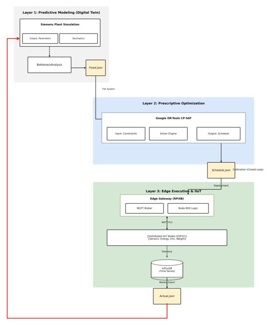
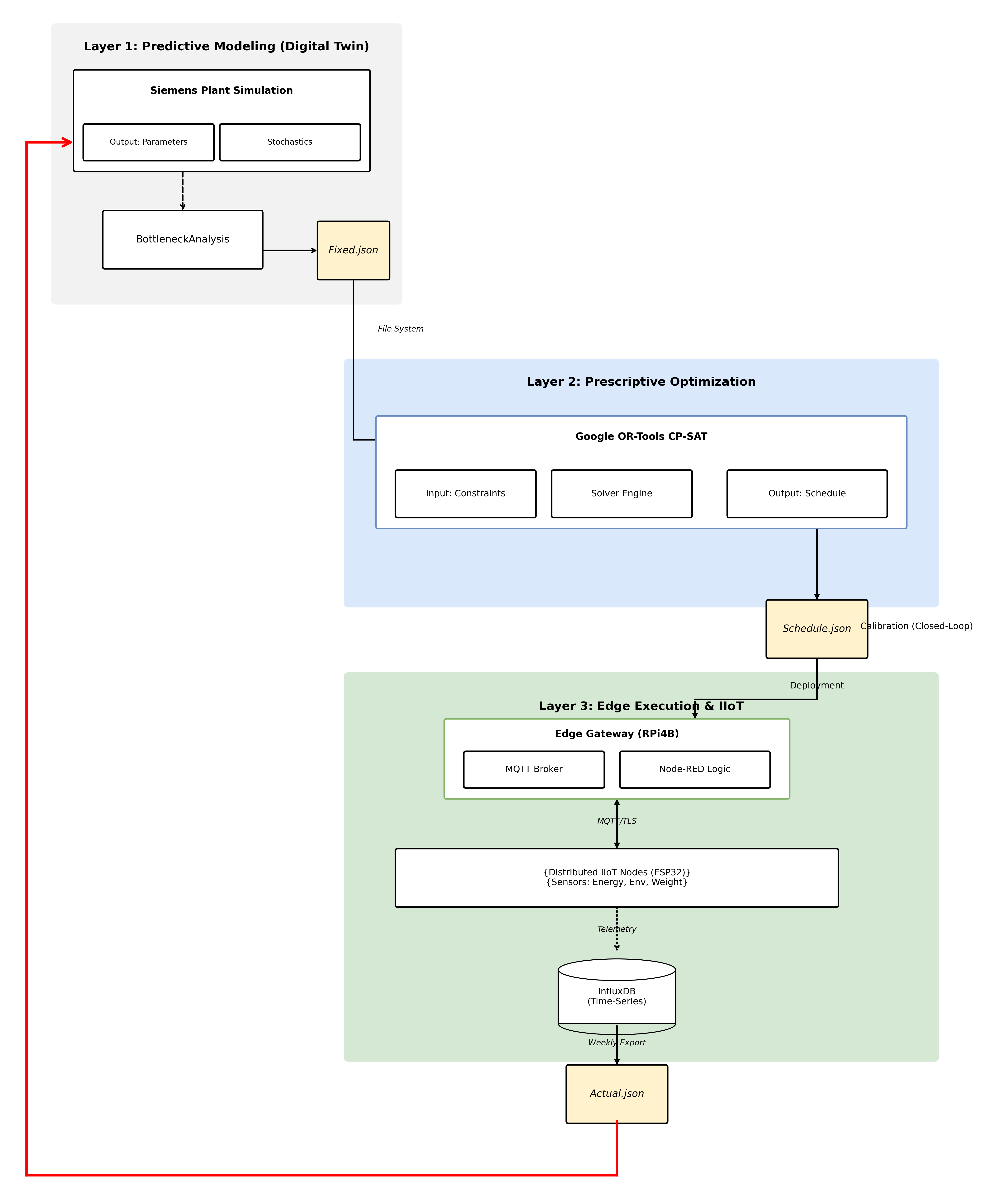
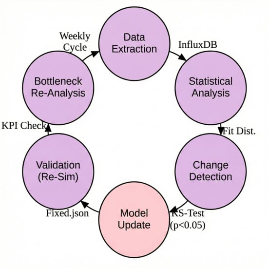
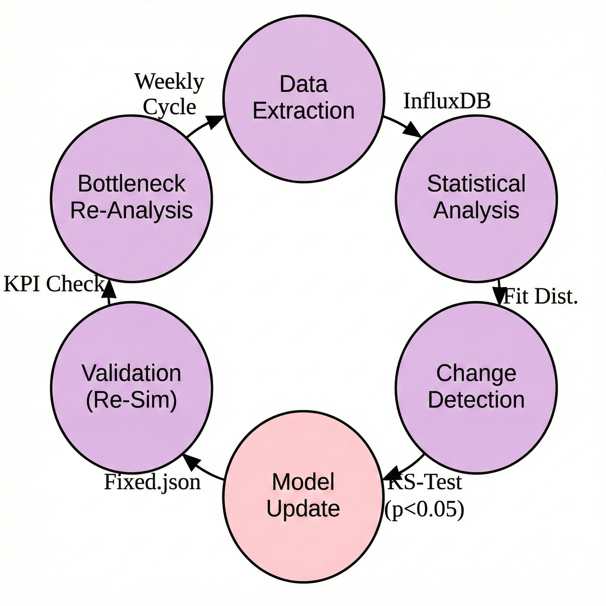
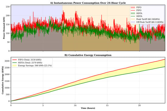
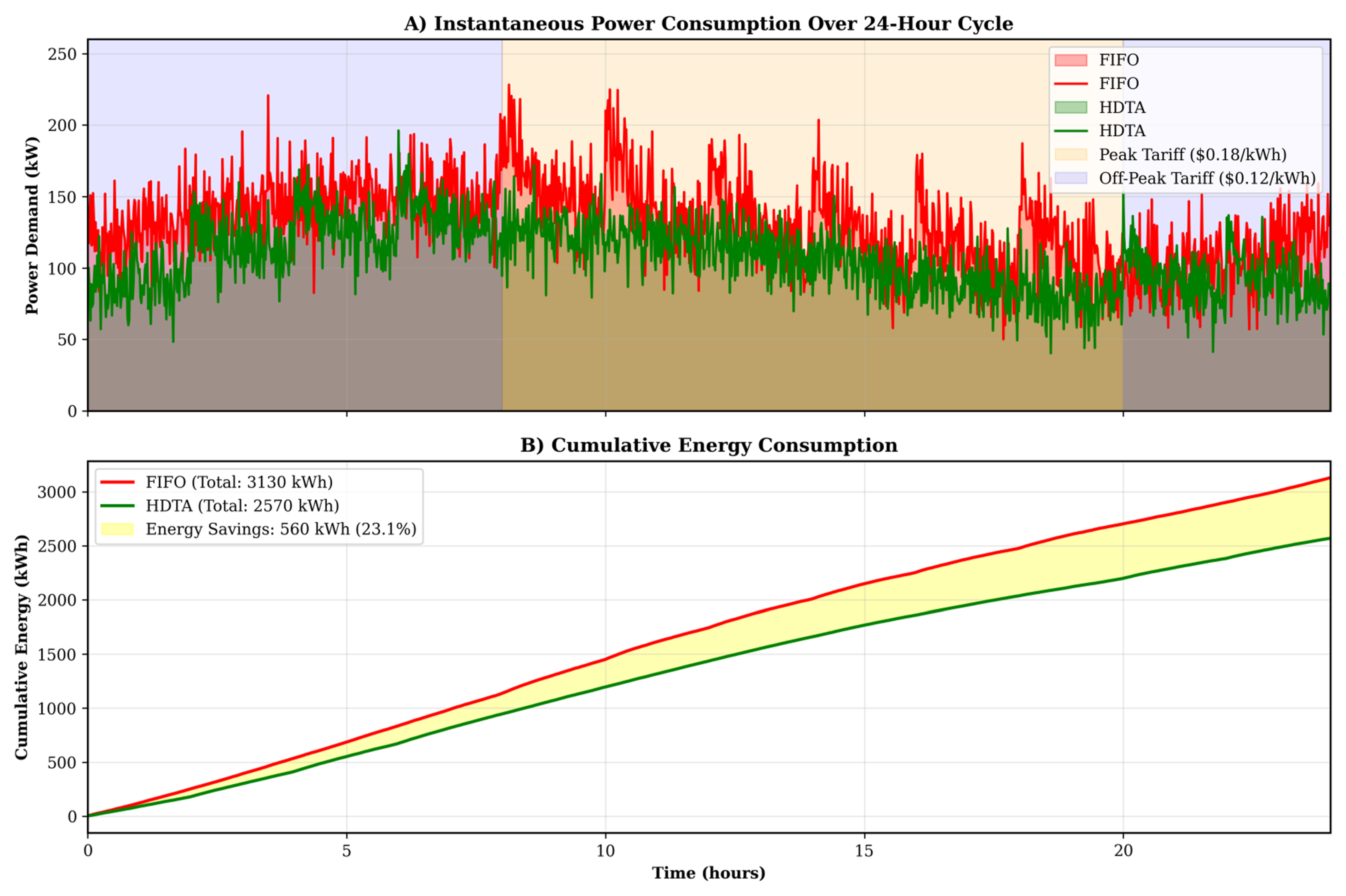
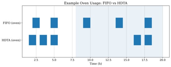
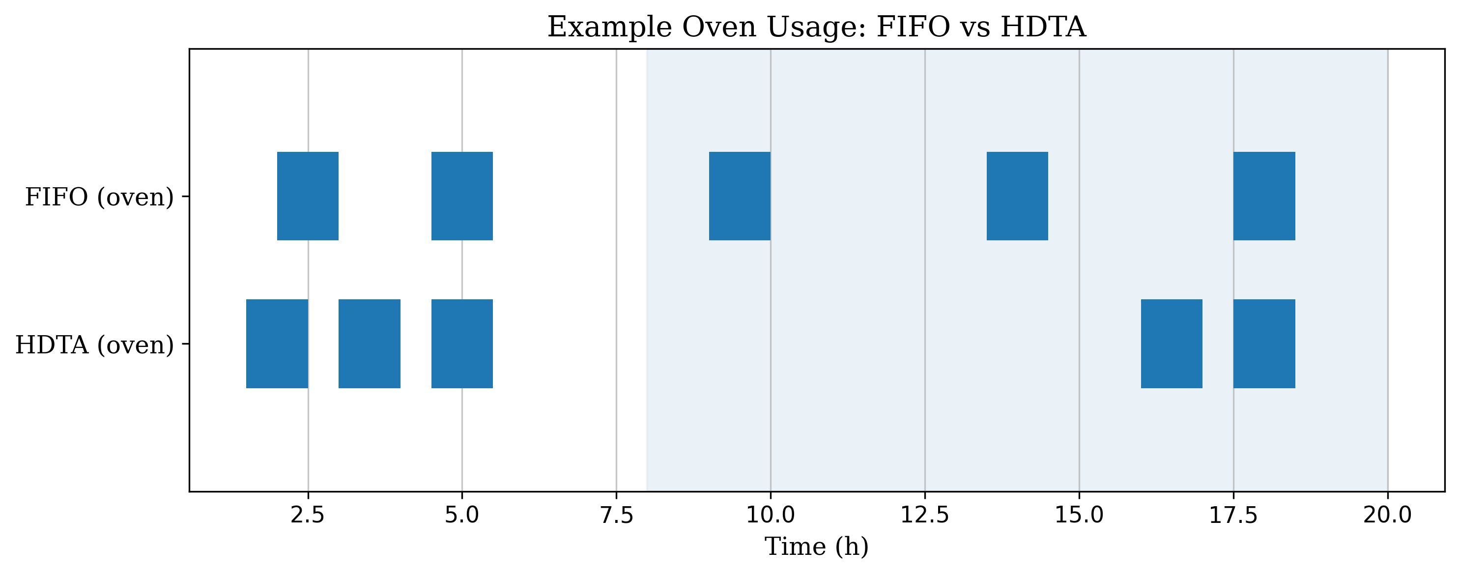
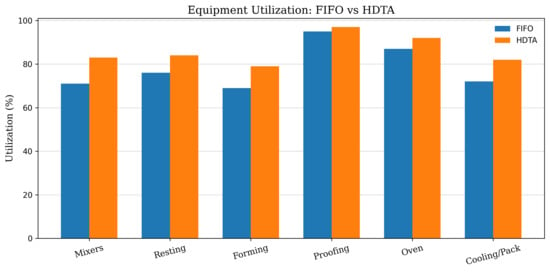
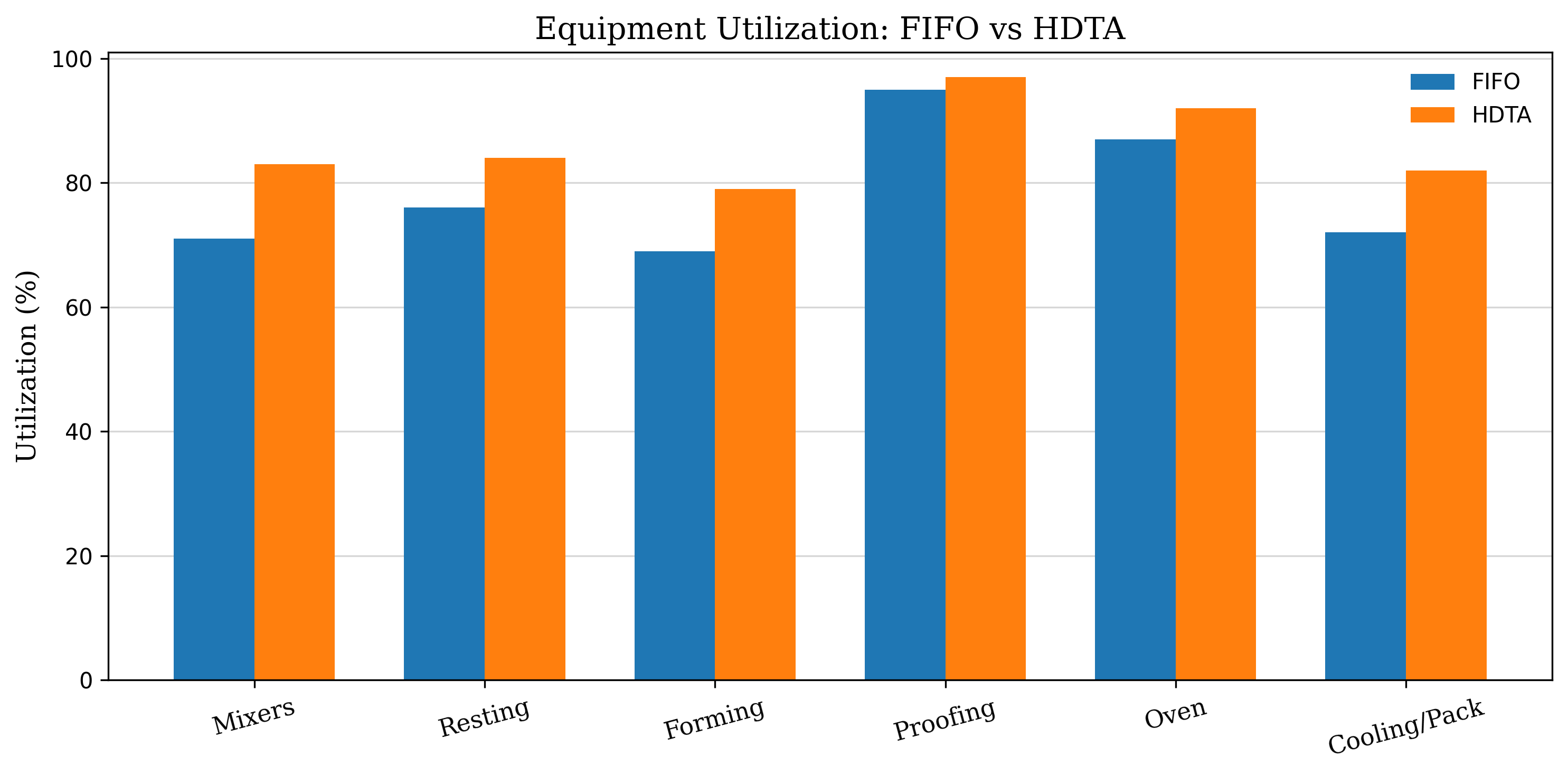
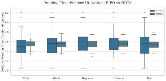
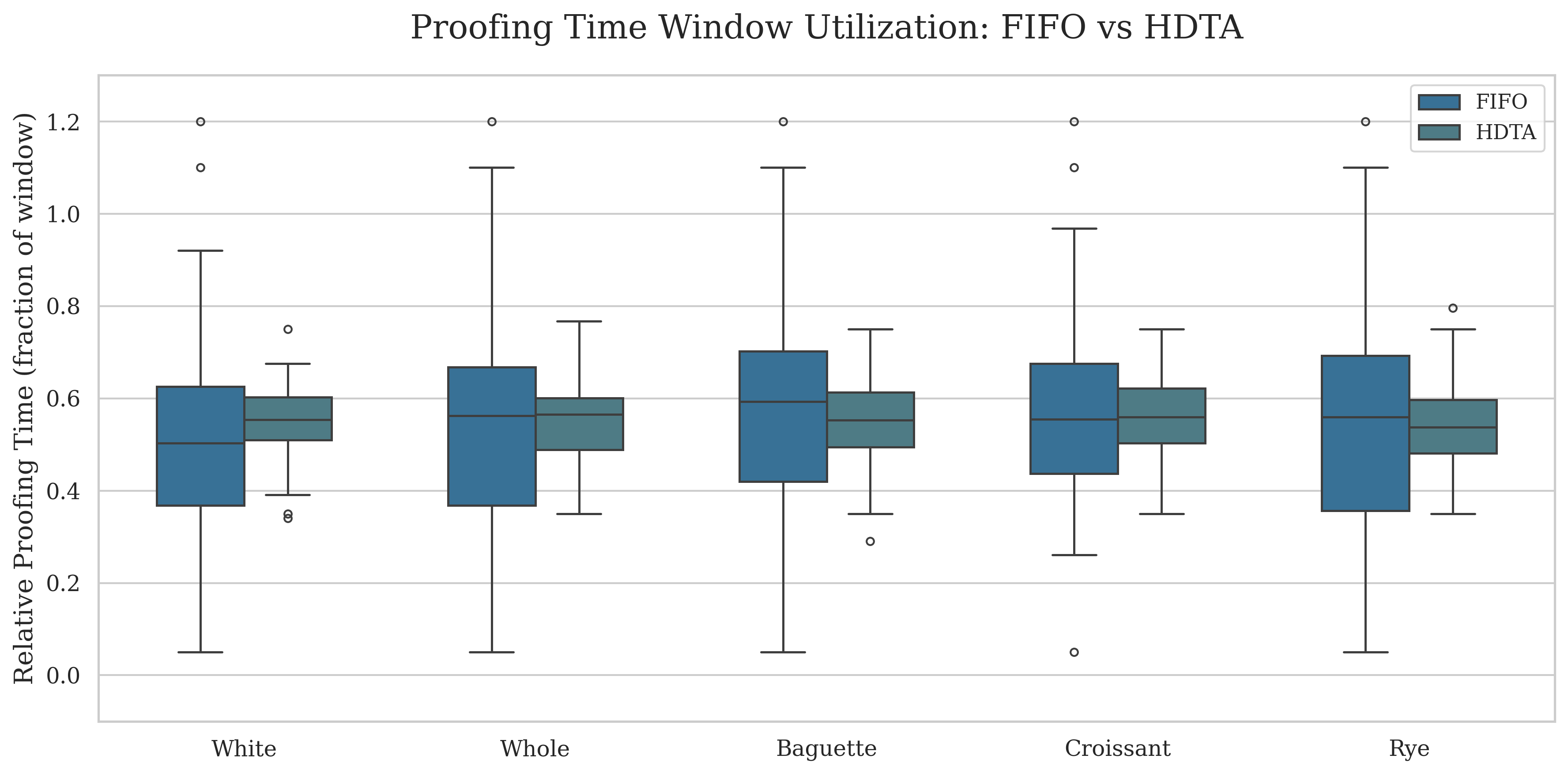
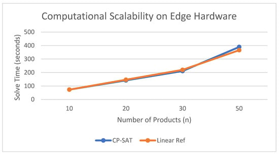
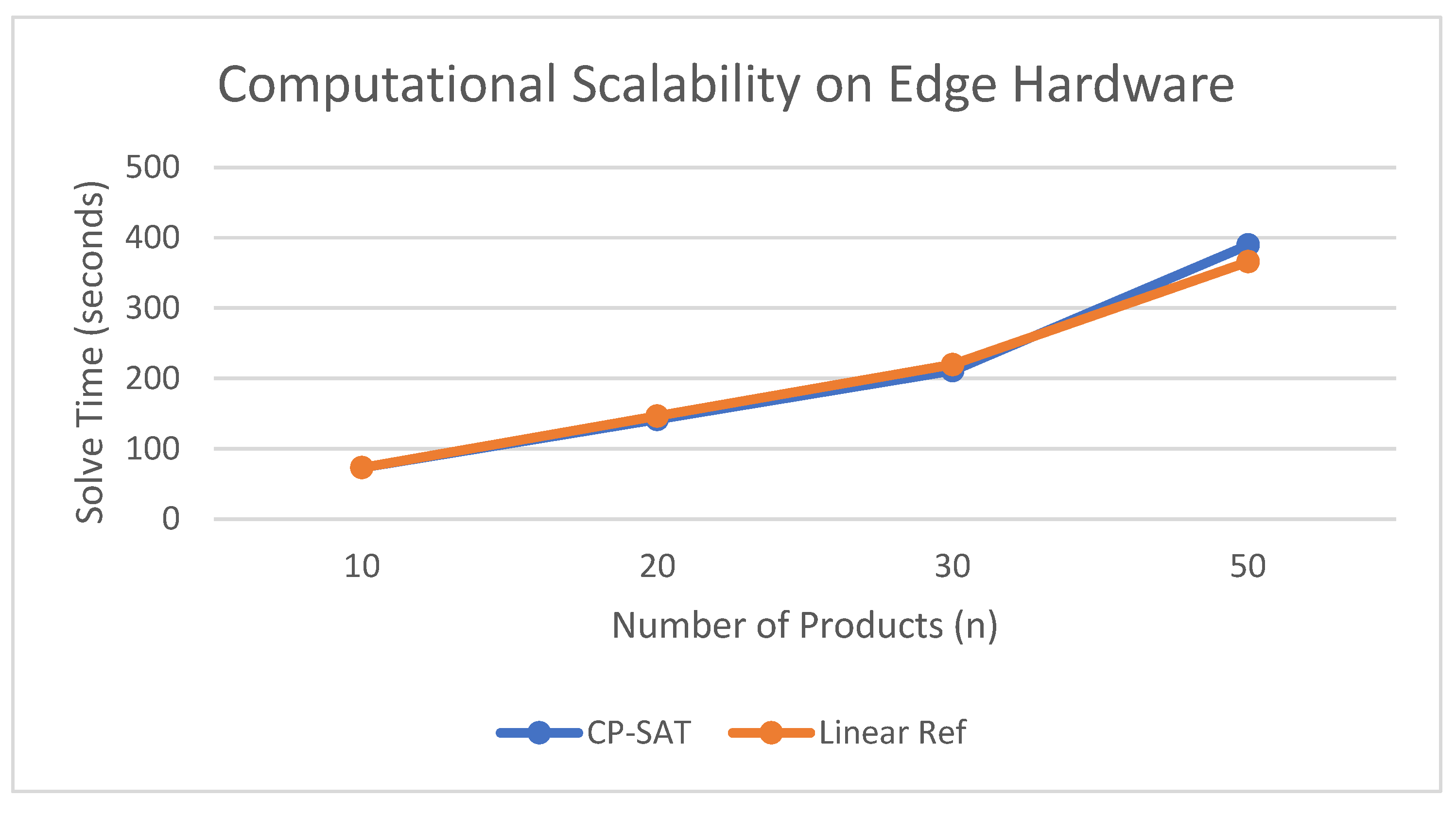
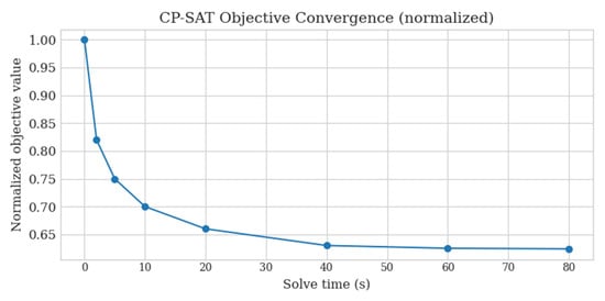
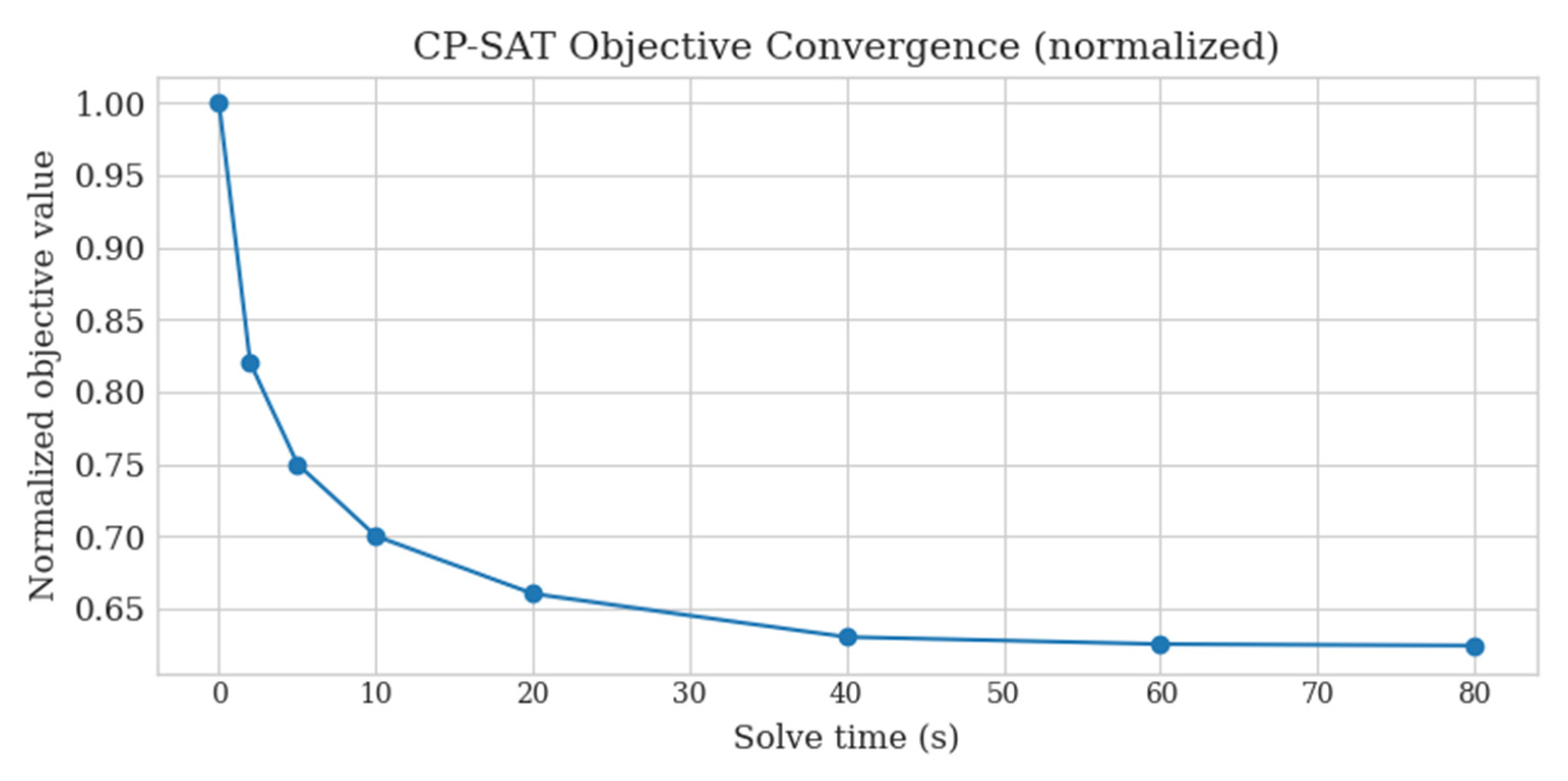

Disclaimer/Publisher’s Note: The statements, opinions and data contained in all publications are solely those of the individual author(s) and contributor(s) and not of MDPI and/or the editor(s). MDPI and/or the editor(s) disclaim responsibility for any injury to people or property resulting from any ideas, methods, instructions or products referred to in the content. |
© 2026 by the authors. Licensee MDPI, Basel, Switzerland. This article is an open access article distributed under the terms and conditions of the Creative Commons Attribution (CC BY) license.