Machine Learning on Small Experimental Datasets in Manufacturing: A Review of Data Leakage, Grouped Validation, and Uncertainty Quantification

Abstract

Machine learning is increasingly used to predict machining and process quality from experimental data, yet such data are typically small, generated by designed experiments, and hierarchically organized, with several measurements taken on the same specimen, tool, or batch. Under these conditions, standard evaluation practice can substantially overstate predictive performance. This review synthesizes the methodological literature from statistics, machine learning, and applied domains to provide guidance for small-data machine learning in manufacturing. We present a taxonomy of data-leakage pathways, compare validation strategies (row-wise, grouped, blocked, nested, and bootstrap-based), discuss model families suited to small tabular data, and review uncertainty-quantification methods, including conformal prediction for grouped data and statistical procedures for comparing models. A reproducible simulation of a specimen–section design shows that row-wise cross-validation increasingly underestimates the error on new specimens as within-specimen correlation grows—whereas grouped cross-validation remains close to it—and that non-nested model selection yields optimistic estimates. Additional experiments with constant total variance, a full-factorial design, and six model families show that the bias is driven by within-specimen dependence and is largest for flexible learners. The review concludes with a reporting checklist and open research directions.

1. Introduction

Machine learning (ML) has become a standard tool for predicting product and process quality in manufacturing, including surface roughness, hardness, residual stresses, dimensional accuracy, and tool wear [1,2,3,4]. In machining in particular, recent reviews document a rapid growth of ensemble, deep, and hybrid models for surface-quality prediction [5,6]. At the same time, these reviews repeatedly identify the same bottleneck: the experimental datasets on which models are trained and evaluated are small, expensive to extend, and specific to a material, tool, and parameter range [5,7,8].

Small size is only part of the problem. Manufacturing datasets are usually generated by designed experiments [9], so their rows are not independent draws from a population: several measurements often belong to the same specimen, tool edge, workpiece, or production batch; factor levels are fixed by design; and several responses are measured on the same object. Under such structure, evaluation procedures that are adequate for large independent datasets—random row-wise splits, preprocessing on the full dataset, or hyperparameter tuning on the test folds—can produce estimates that are overly optimistic [10,11,12]. Kapoor and Narayanan documented leakage-driven errors across hundreds of ML-based studies in many scientific fields [11], and comparable concerns have been raised in genomics, clinical prediction, chemistry, and materials science [13,14,15,16].

In machining research, recent studies have begun to address these issues explicitly, for example, by emphasizing the inadequacy of very small test samples [17], by quantifying predictive uncertainty for small hard-turning datasets [18], and by publishing open experimental data that allow independent re-analysis [19]. Recent hard-turning studies illustrate the breadth of current approaches, from classical ML comparisons and model ensembles to ANN–response-surface hybrids and the estimation of hardness from in-process data [20,21,22,23]. Across the wider literature, however, validation designs vary considerably, and grouped validation, nested model selection, and prediction uncertainty are not yet reported routinely [3,5]. A methodological reference focused on small, structured manufacturing data is therefore needed.

This review addresses that need from a computer-science and statistical-learning perspective. It does not propose a new learning algorithm; instead, it synthesizes and tests evaluation methodology. Its contributions are as follows:

• A taxonomy of data-leakage pathways that are typical of small experimental datasets in manufacturing, with concrete remedies (Section 4).
• A comparative synthesis of validation strategies—row-wise, grouped, blocked, nested, and bootstrap-based—together with guidance on when each is appropriate (Section 5).
• A reproducible simulation of a specimen–section design that quantifies the optimism of row-wise cross-validation and of non-nested model selection, its dependence on the design and the model family, and the coverage of cluster-level prediction intervals (Section 5.4 and Section 7).
• A review of model families, uncertainty-quantification methods, and statistical procedures for comparing models on small data (Section 6, Section 7 and Section 8), followed by a reporting checklist, an implementable evaluation procedure (Algorithm 1), a comparison of evaluation practice in representative manufacturing studies, and open research directions (Section 9 and Section 10).

2. Scope and Review Methodology

This is a narrative methodological review. Literature was identified through searches in Scopus, Web of Science Core Collection, and Google Scholar; the searches were last updated in October 2026. Two groups of queries were combined. Methodological queries targeted titles, abstracts, and keywords; for example, in Scopus: TITLE-ABS-KEY ((“data leakage” OR “cross-validation” OR “nested cross-validation” OR “grouped cross-validation” OR “clustered data” OR “conformal prediction” OR “uncertainty quantification” OR “model comparison”) AND (“machine learning” OR “small data” OR “small sample”)). Application queries combined the terms “machine learning” OR “deep learning” with “machining”, “surface roughness”, “hardness”, or “manufacturing quality” and were restricted to 2022–2026. Equivalent queries were used in Web of Science, and Google Scholar was used to locate foundational works and preprints. Reference lists of key methodological papers were then screened (backward snowballing).

Studies were included if they (i) introduced or analyzed a validation, resampling, uncertainty-quantification, or model-comparison method relevant to small or clustered data; (ii) quantified evaluation bias or leakage empirically; or (iii) reported ML prediction of manufacturing quality from experimental data in a way that illustrates current validation practice. Studies were excluded if they were not peer-reviewed (except widely used methodological preprints and software papers), addressed only large-scale image or sensor streams without a transferable validation issue, or did not describe their evaluation procedure. Priority was given to foundational statistical and ML works, methodological studies that quantify bias, and recent manufacturing applications. Because the aim is to provide methodological guidance rather than to estimate effect sizes across studies, no formal meta-analysis or risk-of-bias scoring was performed, and the review does not claim to be exhaustive.

The review focuses on supervised regression and classification on tabular data with tens to a few thousand observations, which is the typical regime of designed machining experiments. Image-, signal-, and time-series-based monitoring is discussed only where its validation issues are shared with tabular data.

Generative artificial intelligence (Claude, Anthropic) was used to assist in organizing the collected literature, drafting and language-editing the text, and writing the simulation code and figure scripts described in Section 5.4. All cited sources were identified and checked by the authors, the simulation code was executed and its outputs verified, and the authors take full responsibility for the content.

3. Characteristics of Small Experimental Datasets in Manufacturing

Table 1 summarizes the properties that distinguish small experimental manufacturing datasets from the large, independent datasets for which most ML evaluation practice was developed. Four properties are especially consequential.

Table 1. Characteristics of small experimental manufacturing datasets and their methodological consequences.

Characteristic	Typical Manifestation	Consequence for ML Evaluation
Small sample size	Tens to hundreds of rows	High variance of performance estimates; limited power of comparisons
Designed factor structure	Few discrete levels; each combination once	Splits must respect the design; extrapolation must be identified
Clustered observations	Several measurements per specimen, tool, or batch	Row-wise splits leak cluster information; grouped resampling required
Multiple responses	Roughness, hardness, stresses, wear	Target-wise metrics and normalization; possibly different models per target
Temporal or sequential order	Tool wear progression; batches over time	Blocked or forward-chaining splits
Measurement noise	Instrument and repeatability error	Lower bound on achievable error; need for uncertainty estimates

Designed factor structure. Process parameters are usually set at a few discrete levels in full or fractional factorial, Taguchi, or response-surface designs [9]. The input space is therefore sparsely and regularly sampled, and every combination may occur only once. Prediction for a new parameter combination is an interpolation (or extrapolation) task across the design grid, not a draw from a dense empirical distribution.

Hierarchical (clustered) observations. Several measurements are frequently made on the same physical unit—for example, several sections of a specimen machined at different depths of cut, several roughness traces on one workpiece, or several parts produced with the same tool edge. Measurements within a cluster share unobserved factors such as material microstructure, setup, or tool condition and are therefore correlated. The strength of this dependence can be summarized by the intraclass correlation coefficient as follows [24,25]:

$$\mathrm{I}\mathrm{C}\mathrm{C}={\displaystyle \frac{{\sigma }_b^2}{{\sigma }_b^2+{\sigma }_{\epsilon }^2}},$$

(1)

Here, σ_b² is the between-cluster variance, and σ_ε² is the within-cluster (residual) variance. Values close to one indicate that observations within a cluster carry largely redundant information. In designed experiments, two versions of the ICC must be distinguished. An unadjusted ICC, estimated from a random-intercept model of the raw response, attributes to the between-cluster variance both the effects of the deliberately varied factors and the unexplained specimen-to-specimen variation. A conditional ICC, estimated from a mixed model that includes the design factors as fixed effects, retains only the unexplained part. The latter is the quantity that governs dependence leakage, because a model can learn the factor effects but not the unexplained specimen effects; the unadjusted ICC is therefore an upper bound. Open datasets such as the hard-turning data of [19], with 27 specimens and three sections each, allow both versions to be computed, and studies should report the variance components and state which version is given.

Multiple, physically different responses. Roughness, hardness, residual stress, and tool wear are often measured on the same specimens. They may depend on different subsets of factors and differ in scale and noise level, so that multi-output modeling, target-wise normalization, and per-target reporting become necessary [3]. Typical examples are experimental studies in which surface roughness and microhardness are measured on the same small set of specimens, such as the finishing of gear teeth with a shaver-rolling tool [26,27] and the rotary multi-blade turning of rod-type parts of hydraulic impulse systems [28]; such studies provide valuable physical insight but contain only a few independent specimens, which is precisely the regime addressed in this review. They are cited here as concrete examples of the data structure discussed in this section rather than as ML studies: in each of them, roughness or microhardness is measured repeatedly on the same tooth, section, or specimen, so the measurements form clusters, and several responses are recorded on the same physical units. A model trained on such data would therefore require grouped validation at the specimen level.

Small effective sample size. Because of clustering, the effective number of independent units is closer to the number of clusters than to the number of rows. A dataset with 81 rows from 27 specimens contains far less independent information than 81 independent observations. This limits the precision of any performance estimate and the power of any model comparison [29].

4. Data Leakage: A Taxonomy for Small Experimental Data

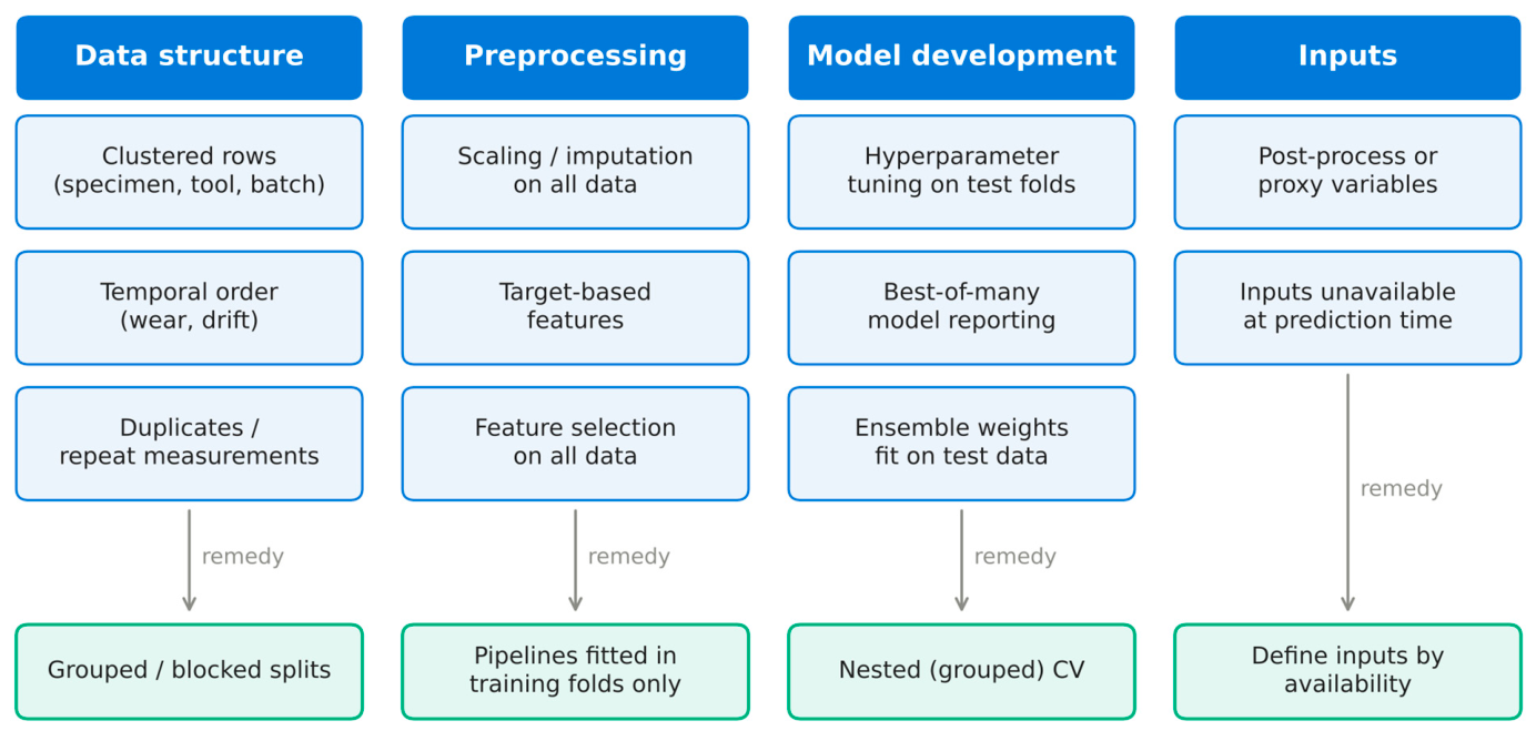
Data leakage occurs when information that would not be available at prediction time influences model training or model selection, so that the evaluation no longer reflects the intended use [10]. In a large-scale survey, Kapoor and Narayanan identified eight types of leakage, ranging from missing train–test separation to non-independence between training and test samples [11]. Figure 1 and Table 2 organize the pathways that are most relevant to small experimental datasets.

Figure 1. Pathways of data leakage in small experimental datasets, grouped by the stage of the modeling workflow at which they occur, with the corresponding remedies.

Dependence leakage. A pathway that is particularly relevant to designed manufacturing experiments, because several measurements are routinely taken on each specimen, is non-independence between training and test data. When sections of the same specimen, or parts machined with the same tool edge, appear in both the training and test partitions, the model can exploit shared cluster-specific information that will not be available for a new specimen. This leads to optimistic estimates whose magnitude grows with the intraclass correlation (Section 5.4). The phenomenon is well documented as record-wise versus subject-wise validation in clinical ML [14], as the motivation for blocked cross-validation in ecology [30], and as the motivation for leave-one-cluster-out validation in materials discovery [31]. The same problem arises in signal-based process monitoring, where a few independent machining experiments can yield thousands of overlapping signal windows. In a study on the detection of geometrical defects in wire electrical discharge machining, for example, about 20,000 in-process records sampled every 5 ms were divided into 15,000 training and 5000 test records [32]; when such records originate from the same cut or workpiece, consecutive windows are strongly correlated, and the independent unit for validation is the experiment, not the signal fragment. Cross-validation should therefore be organized by experiment, and the number of independent experiments should be reported alongside the number of extracted samples.

Preprocessing leakage. Standardization, imputation, outlier removal, feature construction based on target statistics, and dimensionality reduction must be fitted on the training partition only. Fitting them on the full dataset transfers information about the test data into the model. In small datasets, even means and variances can differ noticeably between folds, so the effect is not negligible [11,33].

Selection leakage. When features, hyperparameters, or model families are selected using the same data that are then used to report performance, the reported performance is optimistically biased. This selection bias can be of the same order as the differences between learning algorithms [34,35,36]. It also arises implicitly when many models are compared on the same folds and only the best is reported.

Temporal leakage. When tool wear or process drift creates temporal dependence, random splits allow the model to learn from the “future”. Forward-chaining or blocked splits are then required [37,38].

Target and proxy leakage. Inputs that are measured after or together with the target, or that are deterministic functions of it, make prediction trivial. Typical examples in machining are using one roughness parameter (e.g., R_z) to predict another (R_a), or using post- measurements as inputs for a model intended to support process decisions made before machining.

Table 2. Leakage pathways in small experimental datasets and recommended remedies.

Pathway	Example in Manufacturing	Remedy
Dependence (cluster)	Sections of one specimen in both train and test	Grouped splits by specimen, tool, or batch [14,30]
Preprocessing	Scaler or imputer fitted on all data	Fit all transformations inside each training fold (pipelines)
Feature selection	Features ranked by correlation on full data	Perform selection inside the inner loop of nested CV [34]
Hyperparameter/model selection	Best of many models reported on the same folds	Nested CV or an untouched test set [35,36]
Temporal	Random split of tool-wear sequence	Forward-chaining or blocked splits [37]
Target/proxy	Rz used to predict Ra	Define inputs by availability at prediction time
Duplicate/near-duplicate rows	Repeated measurements of one condition	Aggregate or group repeated measurements

Table 2. Leakage pathways in small experimental datasets and recommended remedies.

Pathway	Example in Manufacturing	Remedy
Dependence (cluster)	Sections of one specimen in both train and test	Grouped splits by specimen, tool, or batch [14,30]
Preprocessing	Scaler or imputer fitted on all data	Fit all transformations inside each training fold (pipelines)
Feature selection	Features ranked by correlation on full data	Perform selection inside the inner loop of nested CV [34]
Hyperparameter/model selection	Best of many models reported on the same folds	Nested CV or an untouched test set [35,36]
Temporal	Random split of tool-wear sequence	Forward-chaining or blocked splits [37]
Target/proxy	Rz used to predict Ra	Define inputs by availability at prediction time
Duplicate/near-duplicate rows	Repeated measurements of one condition	Aggregate or group repeated measurements

5. Validation Strategies

5.1. Row-Wise, Grouped, and Blocked Cross-Validation

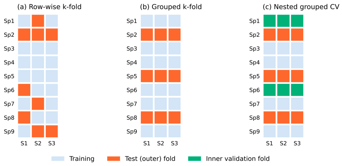
k-fold cross-validation (CV) estimates prediction error by repeatedly training on k − 1 folds and testing on the remaining fold [39,40,41]. Its validity rests on the assumption that the held-out fold is exchangeable with future data. For clustered data, this assumption holds only if entire clusters are assigned to folds (grouped or cluster CV); row-wise assignment estimates the error for new measurements on already seen clusters, which is usually not the quantity of interest [14,30]. Figure 2 contrasts the schemes for a specimen–section design. When clusters are also ordered in time, blocked or forward-chaining schemes are needed [37]. In materials and chemistry, leave-one-cluster-out and scaffold or time splits play the same role for extrapolation to new families of materials or compounds [31,38].

Figure 2. Validation schemes for a specimen–section design (rows: specimens; columns: sections). (a) Row-wise k-fold: sections of one specimen are split between training and test folds. (b) Grouped k-fold: complete specimens are held out. (c) Nested grouped CV: an outer grouped split estimates performance, and inner grouped splits within the outer training set are used for tuning and selection.

Even correctly specified CV has limitations. Bates, Hastie, and Tibshirani showed that CV estimates the average error of models fitted on other training sets drawn from the same population rather than the error of the specific fitted model, and that naive CV confidence intervals can undercover [42]. For small datasets, the variance of the CV estimate is substantial, and repeated CV with different fold assignments, together with an explicit report of fold-to-fold variability, is advisable [29,36].

5.2. Nested Cross-Validation

When a modeling pipeline involves any data-driven choice—feature selection, hyperparameter tuning, model-family selection, or ensemble weighting—the performance estimate must be obtained from data that were not used for those choices. Nested CV achieves this by embedding an inner CV loop, used only for selection, within each outer training partition [34,35,43]. For clustered data, both loops must be grouped. The outer-loop estimate is as follows:

$${\widehat{E}}_{\mathrm{n}\mathrm{e}\mathrm{s}\mathrm{t}\mathrm{e}\mathrm{d}}={\displaystyle \frac{1}{K}}\sum _{k=1}^K{\displaystyle \frac{1}{\left|{\mathcal{D}}_k\right|}}\sum _{(x_i,y_i)\in {\mathcal{D}}_k}L\left(y_i,{\widehat{f}}_{{\widehat{\theta }}^{(-k)}}\left(x_i\right)\right),$$

(2)

Here, K is the number of outer folds; ${\mathcal{D}}_{\mathrm{k}}$ is the k-th outer test fold, consisting of complete clusters, with |${\mathcal{D}}_{\mathrm{k}}$| being the number of observations in it; ${\mathcal{D}}^{(-\mathrm{k})}$ is the corresponding outer training set; (x_i, y_i) are the input vector and the measured response of observation i; ${\widehat{\mathsf{\theta }}}^{(-\mathrm{k})}$ denotes the configuration (model family and hyperparameters) selected by the inner grouped CV using only ${\mathcal{D}}^{(-\mathrm{k})}$; ${\widehat{\mathrm{f}}}_{{\widehat{\mathsf{\theta }}}^{(-\mathrm{k})}}$ is the model with this configuration refit on ${\mathcal{D}}^{(-\mathrm{k})}$; and L is the loss function, for example, the squared error L(y, ŷ) = (y − ŷ)², whose square root after averaging gives the RMSE.

Note that nested CV evaluates the entire modeling procedure, including the selection step, rather than a single fixed model [35,36].

5.3. Bootstrap and Cluster Bootstrap

Bootstrap estimators such as the .632+ bootstrap offer an alternative with lower variance for small samples [44], and bootstrap resampling is also widely used to quantify the uncertainty of performance metrics and rankings [45]. For clustered data, resampling must be performed at the cluster level—i.e., whole specimens are drawn with replacement [46]. With few clusters, cluster-bootstrap intervals can be too narrow; studies of cluster-robust inference report noticeable undercoverage with fewer than about 20–30 clusters [47], so the threshold in Table 3 should be read as a practical guideline rather than a strict requirement, and with fewer clusters the intervals should be interpreted cautiously or complemented by exact permutation procedures. A cluster bootstrap of out-of-fold predictions provides confidence intervals for metrics and for the probability that a given model ranks first, which is more informative than a single ranking when several models perform similarly.

Table 3. Comparison of validation strategies for small experimental datasets.

Strategy	Estimates	Appropriate When	Main Risk
Single random split	Error on one test set	Large, independent data	High variance; dependence leakage
Row-wise k-fold CV	Error for new rows of seen clusters	Rows are independent	Optimistic for clustered data
Grouped k-fold/LOGO CV	Error for new clusters	Several rows per specimen, tool, or batch	Higher variance; fewer training clusters
Blocked/forward-chaining CV	Error for future data	Temporal drift or wear	Requires sufficient sequence length
Nested (grouped) CV	Error of the whole procedure incl. selection	Any tuning or model selection	Computational cost
Cluster bootstrap	Uncertainty of metrics and ranks	Comparing models; small samples	Unreliable with few clusters (practical guideline: ≳20)

LOGO, leave-one-group-out.

5.4. Simulation: How Large Is the Optimism?

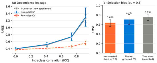
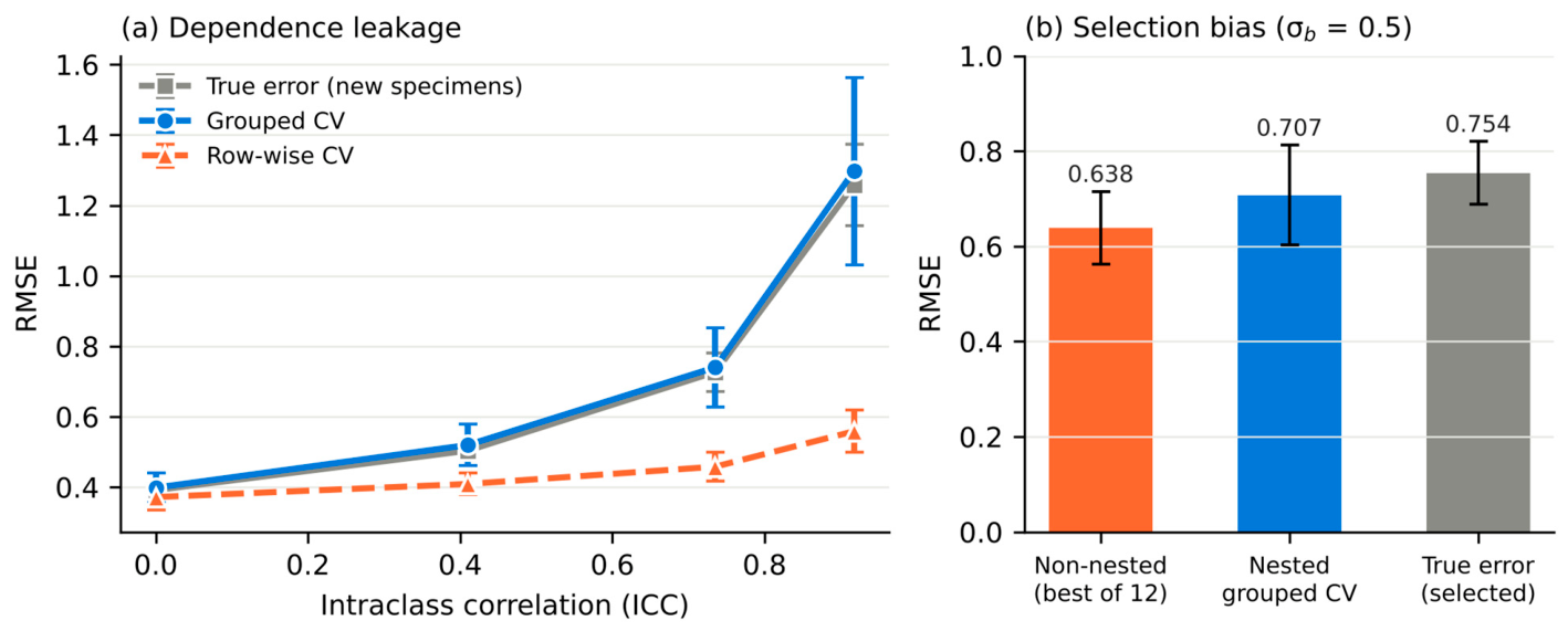
To illustrate the magnitude of the effects discussed above, a small simulation was performed that mimics a typical hard-turning design: 27 specimens, each with three between-specimen factors drawn uniformly from [−1, 1] and three sections at depth-of-cut levels {−1, 0, 1}. The response combined a nonlinear function of the factors with a specimen-level random effect of standard deviation σ_b and residual noise with σ_ε = 0.3. A random forest [48] was evaluated by nine-fold row-wise CV and nine-fold grouped CV, and its true error was computed on new, independently generated specimens. Each setting was replicated 40 times (Figure 3a); the selection experiment below used 20 replications because of the cost of nested CV (Figure 3b). All computations used scikit-learn (version 1.9.1) [49]; the code is provided as Supplementary Material.

Figure 3. Simulation of a 27-specimen, three-section design. (a) Mean RMSE estimated by row-wise and grouped nine-fold CV versus the true error on new specimens, as a function of the intraclass correlation (ICC); error bars show ±1 SD over 40 replications. (b) Selection bias with σ_b = 0.5: best-of-12 grouped-CV error (non-nested), nested grouped CV, and the true error of the selected configuration (20 replications).

Figure 3a shows the results. Without a specimen effect (ICC = 0), both CV schemes approximated the true error well (row-wise 0.372, grouped 0.398, true 0.392). As the intraclass correlation increased, row-wise CV became increasingly optimistic: at ICC = 0.74, it reported an RMSE of 0.458 against a true error of 0.727, and at ICC = 0.92 the values were 0.558 and 1.258; that is, row-wise CV underestimated the error on new specimens by 56%. Grouped CV remained close to the true error at all levels (0.740 and 1.297, respectively).

A second experiment (Figure 3b; σ_b = 0.5) examined selection bias. Twelve candidate configurations (random forests, k-nearest neighbors, polynomial ridge regression, and support vector regression) were compared by grouped CV. In the non-nested procedure, each configuration was evaluated by nine-fold grouped CV on all 27 specimens; the configuration with the lowest error was selected, and its CV error was reported. The selected configuration was then refitted on all 27 specimens, and its true error was computed on 5 × 27 new specimens. In the nested procedure, each of nine outer grouped folds held out three specimens; within the remaining 24 specimens, four-fold grouped CV selected the configuration, which was refitted on these 24 specimens and used to predict the held-out specimens, so that the selected configuration could differ between outer folds. Reporting the grouped-CV error of the best configuration (non-nested) gave a mean RMSE of 0.638, whereas nested grouped CV gave 0.707 and the true error of the selected configuration on new specimens was 0.754. Across the 20 replications, the mean difference between the estimate and the true error was −0.116 (95% confidence interval −0.162 to −0.070; −14.9% on average) for the non-nested procedure and −0.047 (−0.105 to 0.011; −5.7%) for nested CV, whose interval includes zero. Two caveats apply to this comparison. Nested CV estimates the error of the whole selection procedure applied to 24 specimens, whereas the true error refers to one configuration refitted on 27 specimens; the smaller training sets make nested CV, if anything, slightly pessimistic, so the remaining optimism is not an artifact of training size. In addition, 20 replications give only moderate precision, and the residual difference for nested CV is not statistically distinguishable from zero. These results are illustrative rather than general, but they agree with earlier analyses of dependence and selection bias [14,34,35].

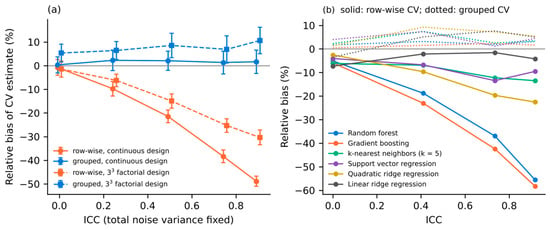
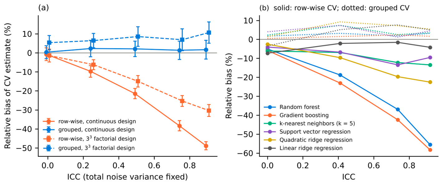
Three additional experiments examined how robust these findings are (Figure 4; code in the Supplementary Materials). First, because increasing σ_b at fixed σ_ε also increases the total variance of the response, the first experiment was repeated with the total noise variance fixed at σ_b² + σ_ε² = 0.34 and only the share of the specimen effect varied (40 replications per level). The relative bias of row-wise CV, (estimate − true error)/true error, then changed from −0.8% (95% CI −4.1 to 2.6%) at ICC = 0 to −21.5% (−24.1 to −18.8%) at ICC = 0.5 and −48.8% (−51.0 to −46.7%) at ICC = 0.9, whereas the bias of grouped CV stayed between 0.3% and 2.2% with confidence intervals that included zero (Figure 4a). The optimism is therefore caused by within-specimen dependence and not by the larger variance of the response.

Figure 4. Robustness of the simulation results. (a) Relative bias of row-wise and grouped nine-fold CV for a random forest when the total noise variance is fixed (σ_b² + σ_ε² = 0.34) and only the ICC varies, for a continuous random design and a 3³ full-factorial design; error bars show 95% confidence intervals of the mean over 40 replications. (b) Relative bias of row-wise (solid) and grouped (dotted) CV for six model families as a function of the ICC (design of Figure 3a, 40 replications).

Second, the same experiment was run with a conventional 3³ full-factorial design, in which the 27 specimens correspond to the 27 combinations of three factors at three levels. Row-wise CV was again increasingly optimistic, although less so than with the continuous design (−30.4%, 95% CI −33.5 to −27.2%, at ICC = 0.9), because with discrete levels every factor setting also occurs in other specimens, so that less specimen-specific information can be exploited. Grouped CV was slightly pessimistic for the factorial design (between +5.3% and +10.6%), because holding out three complete runs removes design points that the model can only extrapolate to. This illustrates that the structure of the design influences both estimators and that, for factorial designs, grouped CV should be regarded as a conservative estimate.

Third, the experiment of Figure 3a was repeated for six model families (Figure 4b). At ICC = 0.92, the relative bias of row-wise CV was −56% for the random forest and −58% for gradient boosting, between −10% and −23% for k-nearest neighbors, support vector regression, and quadratic ridge regression, and only −4% for linear ridge regression; grouped CV stayed within +2% to +5% for all models. Flexible learners that can fit specimen-specific deviations are thus affected most, whereas a strongly constrained model has little capacity to exploit them. Low row-wise optimism for a linear model is therefore not evidence that row-wise CV is adequate for a more flexible model trained on the same data.

The magnitude of the bias observed here should not be transferred directly to other settings. As Figure 4 shows, it depends on the dataset structure (the number of clusters, the number of observations per cluster, and the intraclass correlation), on the model type (flexible learners such as random forests or k-nearest neighbors can exploit cluster-specific information more strongly than heavily regularized linear models), and on the validation design (the number of folds, the size and number of candidate configurations, and whether clusters are balanced). The direction of the effect—optimism of row-wise CV under within-cluster correlation and of non-nested selection—is supported by theory and by the studies cited above, whereas its size in a particular application should be assessed by comparing row-wise and grouped estimates on the data at hand.

5.5. Classification Tasks

The examples above concern regression, but the same principles apply when the target is categorical, for example, conforming versus nonconforming parts, tool-wear states, or surface-defect classes. Three issues deserve particular attention in small datasets. First, class imbalance is common because defective outcomes are rare; folds should then be both grouped and stratified so that every outer and inner fold contains each class, any resampling or class weighting must be applied within the training folds only, and accuracy should be replaced or complemented by metrics that remain informative under imbalance, such as balanced accuracy, the Matthews correlation coefficient, or the area under the precision–recall curve [50,51,52]. Second, grouped metrics are needed when a decision concerns a whole specimen or batch: in addition to row-level metrics, the classification of the independent unit (e.g., by majority vote or by the maximum predicted defect probability across its measurements) should be evaluated and reported with the number of units. Third, probability calibration matters whenever predicted probabilities are used for decisions; calibration methods such as Platt scaling or isotonic regression must be fitted on held-out clusters inside the CV loop, and calibration should be reported with the Brier score or reliability diagrams [53]. With few clusters, isotonic regression tends to overfit, and simple parametric calibration is usually preferable [53].

6. Model Families for Small Tabular Data

Benchmarks on medium-sized tabular datasets have shown that tree-based ensembles remain highly competitive with, and often superior to, deep learning [54,55], although carefully designed architectures such as the FT-Transformer narrow the gap [56]. For the very small datasets typical of designed experiments, model choice is dominated by the bias–variance trade-off and by how well the inductive bias matches the physics of the process. Table 4 summarizes the main families.

Table 4. Model families for small tabular manufacturing data.

Family	Strengths	Limitations	Typical Use
Regularized/polynomial regression	Interpretable; stable; matches response-surface designs	Limited nonlinearity	Baseline; DOE analysis
Mixed-effects models	Model cluster effects explicitly	Parametric assumptions	Clustered data baseline
Gaussian process regression	Smooth interpolation; predictive variance	Kernel choice; scaling to large n	Very small data with uncertainty
Tree ensembles/boosting	Interactions; little preprocessing	Poor extrapolation; overfitting with few clusters	Strong general baseline
Tabular neural networks	Flexible; multi-output	Data-hungry; tuning-sensitive	Larger or pooled datasets
TabPFN (foundation model)	No tuning; strong small-data accuracy	Limited evidence for grouped designs	Emerging alternative
Physics-informed/hybrid	Lower data needs; physical consistency	Requires domain models	Processes with known mechanisms

Regularized and polynomial regression (ridge, lasso, elastic net) [41,57] are well suited to response-surface designs, are interpretable, and are difficult to overfit when the number of terms is controlled. Mixed-effects models [25] explicitly model random cluster effects and are a natural baseline whenever data are clustered; they also separate between- and within-cluster variability. Gaussian process regression [58] provides smooth interpolation with built-in predictive uncertainty and has been used successfully for small hard-turning datasets [18]. Tree ensembles and gradient boosting [48,59,60] capture interactions with little tuning but extrapolate poorly beyond the design range and can overfit when the number of clusters is small.

Neural networks for tabular data require careful regularization and early stopping on small data, and their advantage over ensembles is rarely established in this regime [54,55]. A notable recent development is TabPFN, a transformer pre-trained on synthetic datasets that performs in-context prediction and has shown strong accuracy on datasets with up to about ten thousand samples [61]; its behavior on clustered experimental data with grouped validation remains to be studied. Physics-informed and knowledge-informed models embed known relationships—such as kinematic roughness or material laws—as features, constraints, or residual structures [62,63], which can reduce data requirements. Suitable sources of such knowledge include mathematical models of machine and process dynamics, for example, models of hydraulic impulse and percussion mechanisms and of the control of their operating modes [64,65], whose outputs can serve as physically meaningful input features or as simulated pre-training data. For instance, such models relate controllable parameters such as supply pressure or stroke frequency to the impact energy and force acting on the tool, and these derived quantities could replace raw machine settings as inputs to a data-driven model, reducing the number of parameters that must be learned from a small experimental dataset. Transfer learning from related materials, tools, or simulations is another route to compensate for small data [7,8,66]. Finally, stacking and ensembles [67] can improve robustness, but every weighting or selection step must be included in the nested validation loop.

7. Uncertainty Quantification

Point predictions from small datasets are inherently uncertain, and decisions on process parameters require an indication of reliability. Uncertainty comprises an aleatoric component, due to measurement noise and unobserved variability, and an epistemic component, due to limited data and model choice [68,69]. In small experimental datasets, epistemic uncertainty is often dominant, especially near the boundaries of the design.

Model-based approaches include Gaussian process predictive variance [58], Bayesian and mixed-effects models [25], quantile regression [70] and quantile regression forests [71], deep ensembles [72], and Monte Carlo dropout [73]. Their intervals are only as reliable as the underlying model assumptions, and modern neural networks in particular are often miscalibrated [74]. The main uncertainty-quantification methods are summarized in Table 5.

Conformal prediction provides distribution-free intervals with finite-sample coverage guarantees under exchangeability [75,76,77]. In split-conformal regression, absolute residuals on a calibration set serve as nonconformity scores, and the interval is as follows:

$$\widehat{C}\left(x\right)=\left[\widehat{f}\left(x\right)-\widehat{q},\widehat{f}\left(x\right)+\widehat{q}\right],$$

(3)

Here, x is a new input vector, $\widehat{\mathrm{f}}$ is the model fitted on the proper training set, and Ĉ(x) is the prediction interval for the unobserved response y. $\widehat{\mathrm{q}}$ is the ⌈(n + 1)(1 − α)⌉-th smallest of the n calibration scores s_j = |y_j − $\widehat{\mathrm{f}}$(x_j)|, j = 1, …, n, computed on a calibration set that was not used for fitting; α is the target miscoverage level (e.g., α = 0.1 for 90% intervals). Under exchangeability, the interval contains y with probability at least 1 − α.

Variants such as CV+ and the jackknife+ use all data for both training and calibration, which is valuable for small samples [78], and conformalized quantile regression adapts interval width to local difficulty [79]. For clustered data, exchangeability holds between clusters but not between rows, so calibration must be performed at the cluster level. Dunn, Wasserman, and Ramdas developed prediction sets for such two-layer hierarchical models [80]; a simple practical variant uses, for each calibration cluster g, the score as follows:

$$s_g=\underset{i\in g}{\max }\left|y_i-\widehat{f}\left(x_i\right)\right|,$$

(4)

Here, g indexes the calibration clusters (e.g., specimens), i ∈ g runs over the observations of cluster g, and s_g is the largest absolute residual within that cluster. Using $\widehat{\mathrm{q}}$—computed from the cluster scores s_g—in place of the row-wise scores in Equation (3) yields intervals that cover all observations of a new cluster jointly with the nominal probability.

The cost of such guarantees is interval width: with few clusters, valid intervals are necessarily wide, and reporting their empirical coverage and normalized width on held-out clusters is essential.

The number of calibration clusters sets a hard lower limit. The quantile index ⌈(n + 1)(1 − α)⌉ in Equation (3) does not exceed n only if n ≥ (1 − α)/α; for α = 0.1, at least nine calibration units are required, and with eight or fewer the distribution-free interval is unbounded. When cluster-level scores are used, n is the number of calibration clusters, not rows: with 27 specimens, reserving nine for calibration leaves only 18 for training, and the guarantee is then exactly at its limit. Two kinds of coverage must also be distinguished. Marginal coverage refers to a single new observation, whereas simultaneous coverage requires that all observations of a new specimen fall inside their intervals. Row-level calibration targets the former; the cluster-maximum scores of Equation (4) target the latter.

A small simulation illustrates these limits (design of Figure 3a with σ_b = 0.5, random forest, α = 0.1, 300 replications, 200 new test specimens per replication). With eight calibration specimens, the cluster-level interval was unbounded in all replications, while row-level calibration on the 24 rows of these specimens gave a marginal coverage of 0.90 but covered all three sections of a new specimen in only 82% of cases. With nine calibration specimens, cluster-level calibration achieved a simultaneous coverage of 0.90 (marginal coverage 0.95) with a mean interval width of 3.15, compared with 2.73 for row-level calibration, whose simultaneous coverage was 0.84. With twelve calibration specimens, the corresponding values were 0.92 and 3.32 versus 0.83 and 2.66. Simultaneous coverage for a whole specimen is therefore attainable on such small datasets only with wide intervals and a sufficient number of calibration specimens; when fewer are available, CV+ or jackknife+ with cluster-level folds [78], model-based intervals with explicitly stated assumptions, or a lower nominal coverage should be considered and reported as such.

Table 5. Uncertainty-quantification methods for small datasets.

Method	Type	Guarantee	Remark for Clustered Data
Gaussian process variance	Model-based	If model is correct	Add cluster-level kernel or random effect
Mixed-effects prediction intervals	Model-based	If model is correct	Separates within- and between-cluster variance
Quantile regression (forests)	Model-based	Asymptotic	Fit quantiles with grouped tuning
Deep ensembles/MC dropout	Approximate Bayesian	None in general	Often miscalibrated on small data
Split/CV+/jackknife+ conformal	Distribution-free	Finite-sample marginal	Calibrate on whole clusters
Hierarchical conformal	Distribution-free	Finite-sample, cluster-level	Designed for two-layer data [80]

Table 5. Uncertainty-quantification methods for small datasets.

Method	Type	Guarantee	Remark for Clustered Data
Gaussian process variance	Model-based	If model is correct	Add cluster-level kernel or random effect
Mixed-effects prediction intervals	Model-based	If model is correct	Separates within- and between-cluster variance
Quantile regression (forests)	Model-based	Asymptotic	Fit quantiles with grouped tuning
Deep ensembles/MC dropout	Approximate Bayesian	None in general	Often miscalibrated on small data
Split/CV+/jackknife+ conformal	Distribution-free	Finite-sample marginal	Calibrate on whole clusters
Hierarchical conformal	Distribution-free	Finite-sample, cluster-level	Designed for two-layer data [80]

8. Statistical Comparison of Models

Small datasets rarely allow a clear ranking of several strong models. Standard paired t-tests on CV folds are invalid because training sets overlap; Dietterich analyzed this problem and proposed the 5 × 2 CV test [81], and Nadeau and Bengio proposed a variance correction for resampled t-tests [82]. When several models are compared, multiplicity must be controlled, for example, by the Holm procedure [83]; for comparisons across multiple datasets, nonparametric tests [84] and Bayesian alternatives that estimate the probability of practical equivalence [85] are recommended.

For a single clustered dataset, a practical and transparent approach is to compute per-cluster losses from out-of-fold predictions and to compare models with paired cluster-level tests, such as sign-flip permutation tests [86], complemented by cluster-bootstrap confidence intervals for the difference in error [46] and by the bootstrap probability of each model ranking first. Reporting effect sizes, intervals, and the number of clusters that favor each model is more informative than a single p-value. Equally important is to report negative or inconclusive results: when corrected tests do not separate the leading models, the honest conclusion is that the data do not support a ranking.

The sign-flip test rests on explicit assumptions. Let d_g = ℓ_A,g − ℓ_B,g be the difference in the mean out-of-fold loss of models A and B on cluster g. Under the null hypothesis of equal performance, the test assumes that the d_g are independent across clusters and symmetrically distributed around zero, so that their signs are exchangeable [86]; it then compares the observed mean of d_g with its distribution under random sign changes. Independence between clusters is plausible for the test clusters themselves, but the models that produced the losses are trained on overlapping data in different CV folds. The test is therefore conditional on the realized training sets: it accounts for the variability due to the finite number of test clusters, but not for the variability due to the choice of training data, which is the source of the dependence analyzed by Nadeau and Bengio [82] and by Bates et al. [42]. When the latter is of interest, repeated grouped CV with the corrected resampled t-test [82] or the nested CV procedure of Bates et al. [42] should be used. In all cases, the number of clusters limits the attainable significance: with G clusters, an exact sign-flip test has at most 2^G distinct sign patterns.

9. Reporting Checklist

Reporting guidelines for prediction models in medicine [87] and best-practice guides for ML in chemistry and materials science [15,16] share many requirements with manufacturing applications. Table 6 adapts them to small experimental manufacturing datasets. Algorithm 1 condenses the recommendations of Section 4, Section 5, Section 6, Section 7 and Section 8 into a single evaluation procedure that can be implemented with standard software; it is a synthesis of established methods rather than a new learning algorithm.

Algorithm 1. Leakage-safe evaluation of a modeling procedure on a small clustered dataset.

Input: data (xi, yi, gi), i = 1, …, n, with cluster labels gi (e.g., specimen); candidate configurations Θ; loss L; outer folds K; inner folds J; miscoverage level α.

1. Identify the independent unit and compute the intraclass correlation (Equation (1)) of each response; report the number of rows and the number of clusters.

2. Partition the clusters into K outer folds ${\mathcal{D}}_1$ , …, ${\mathcal{D}}_{\mathrm{k}}$, keeping all rows of a cluster in the same fold (stratified by design factors if possible).

3. For k = 1, …, K: (a) fit all preprocessing steps (scaling, feature construction or selection) on ${\mathcal{D}}^{(-\mathrm{k})}$$\mathrm{only};(\mathrm{b})\mathrm{select}\widehat{\mathsf{\theta }}$(−k) ∈ Θ by grouped J-fold CV within ${\mathcal{D}}^{(-\mathrm{k})}$$;(\mathrm{c})\mathrm{refit}\widehat{\mathrm{f}}$$\mathrm{with}\widehat{\mathsf{\theta }}$(−k) on ${\mathcal{D}}^{(-\mathrm{k})}$ and store out-of-fold predictions for ${\mathcal{D}}_{\mathrm{k}}$ .

4. Compute the nested estimate of Equation (2) and the per-cluster losses; obtain a confidence interval for the error by cluster bootstrap of the per-cluster losses (Section 5.3).

5. If prediction intervals are required, calibrate them on held-out clusters using cluster-level scores (Equation (4)); check that the number of calibration clusters is at least ⌈(1 − α)/α⌉ (Section 7) and report coverage per observation and per cluster.

6. To compare procedures A and B, repeat steps 2–4 with identical folds, compute paired per-cluster loss differences, and apply a sign-flip test with Holm correction for multiple comparisons (Section 8).

7. Fit the final model on all data with the procedure of step 3(b); report the nested estimate from step 4 as its expected error, together with the number of clusters and the range of the design space.

Output: final model; nested error estimate with confidence interval; optional calibrated prediction intervals; paired comparison results.

Table 6. Checklist for reporting ML studies on small experimental manufacturing datasets.

Item	What to Report
Data provenance	Source, design (factors, levels, replicates), measurement methods, open repository or availability
Unit of analysis	Prediction unit (row) and independent unit (specimen, tool, batch); number of each
Dependence	Intraclass correlation or other evidence of clustering; temporal order
Splitting	Grouping variable, number of folds, repetitions, random seeds, fold composition
Preprocessing	All transformations and confirmation that they were fitted within training folds
Selection	Search spaces and the use of nested (grouped) CV or an untouched test set
Baselines	Mean predictor, linear/polynomial and mixed-effects models, at least one ensemble
Metrics	Per-target metrics, normalized metrics for multi-output problems, fold variability
Uncertainty	Confidence intervals for metrics; prediction intervals with empirical coverage and width
Comparison	Paired cluster-level tests with multiplicity correction; ranking stability
Scope	Range of validity (design space); external or prospective validation if available
Code	Code, environment, and out-of-fold predictions in a public repository

10. Open Challenges and Future Directions

To connect these methodological concerns with current practice, Table 7 summarizes the evaluation design of representative manufacturing studies cited in this review, using only the information stated in each publication. The selection is illustrative rather than systematic, so the table cannot estimate how often each problem occurs. It nevertheless shows that the issues discussed in Section 3, Section 4, Section 5, Section 6, Section 7 and Section 8 are documented in recent work rather than being only theoretical: the number of independent specimens or runs is small (typically 27 or fewer); single hold-out splits or random row-wise CV are common; it is often not stated whether repeated measurements, augmented samples, or signal windows from the same run were kept together; tuning is rarely separated from the final test in a nested way; and uncertainty is seldom reported.

Table 7. Evaluation design of representative manufacturing ML studies, as reported in the publications.

Study	Process and Target	Independent Units and Rows	Validation	Tuning/Selection	Uncertainty
Mane et al. [22]	Hard turning of AISI 52100; Ra and temperature (RSM, ANN)	27 runs (Taguchi L27); Ra averaged over three points per run	Single hold-out split (23/4)	ANN size by trial and error; learning rate tuned on validation results	None (point metrics)
Pawanr and Gupta [88]	Dry turning of SDSS 2507 with textured tools; Rz (LSSVM, MGGP)	27 runs (L27), augmented to 81 rows (two synthetic points per run)	Single 80:20 split of augmented data; grouping by run NR	LSSVM grid search with LOOCV; separation from test set NR	NR
Wittich et al. [18]	Hard turning of 51CrV4; residual stress and Ra (Takagi–Sugeno, GPR)	Specimens with three sections each; 54 rows (648 depth-resolved)	Random 10-fold CV; grouping by specimen NR	Preliminary tests; GPR by marginal likelihood; nesting NR	GPR 95% interval; bounded-error method
Kohara et al. [23]	Turning of S45C; surface hardness and residual stress (cutting model + linear regression)	Five feed rates; hardness averaged over five points	NR (fitted R2 reported)	Least squares	NR
Wang et al. [32]	Wire EDM of an Inconel 718 fir-tree slot; geometrical defects (deep learning, in-process signals)	One workpiece, five regions; about 20,000 records sampled every 5 ms	15,000/5000 train/test; split by record or region NR	Epochs selected from an error curve	NR

NR, not reported in the publication; RSM, response surface methodology; ANN, artificial neural network; LSSVM, least-squares support vector machine; MGGP, multi-gene genetic programming; GPR, Gaussian process regression; LOOCV, leave-one-out CV.

Several methodological questions remain open. First, external and prospective validation is rare in manufacturing ML, largely because compatible datasets are scarce; shared benchmark datasets with documented designs, such as open hard-turning data [19], would allow independent re-analysis and comparison. Second, distribution shift between laboratories, machines, tools, and materials is the main threat to transferability, and evaluation protocols that hold out entire machines or materials, analogous to leave-one-cluster-out validation in materials discovery [31], deserve wider use. Third, uncertainty quantification for hierarchical data with very few clusters needs methods that remain informative—narrow enough to be useful—while preserving coverage [78,80]. Fourth, foundation models for tabular data [61] and physics-informed learning [62,63] may reduce data requirements, although manufacturing-specific evidence for this is still limited, and their evaluation on designed, clustered experiments with grouped and nested validation is still largely missing. Finally, multi-output prediction of physically different quality indicators requires metrics and comparison procedures that respect differences in scale and noise between targets [3].

11. Conclusions

Small experimental datasets are the norm rather than the exception in manufacturing ML, and their designed and hierarchical structure makes evaluation more delicate than in large-data settings. The literature and the simulation reviewed here support several practical recommendations: identify the independent unit and validate at that level; keep every data-driven step inside the training folds and, when models are tuned or selected, use nested grouped validation; quantify uncertainty with cluster-level resampling and calibration; compare models with paired, cluster-level, multiplicity-corrected procedures; and report inconclusive comparisons as such. The numerical results of the simulation illustrate these effects for one design and should not be read as general estimates of their size. Following these practices, together with open sharing of data, code, and out-of-fold predictions, would make performance claims in manufacturing ML more reliable and more comparable across studies.

References

- Wuest, T.; Weimer, D.; Irgens, C.; Thoben, K.-D. Machine learning in manufacturing: Advantages, challenges, and applications. Prod. Manuf. Res. 2016, 4, 23–45. [Google Scholar] [CrossRef] [Scilit]
- Wang, J.; Ma, Y.; Zhang, L.; Gao, R.X.; Wu, D. Deep learning for smart manufacturing: Methods and applications. J. Manuf. Syst. 2018, 48, 144–156. [Google Scholar] [CrossRef] [Scilit]
- Tercan, H.; Meisen, T. Machine learning and deep learning based predictive quality in manufacturing: A systematic review. J. Intell. Manuf. 2022, 33, 1879–1905. [Google Scholar] [CrossRef] [Scilit]
- Kim, D.-H.; Kim, T.J.Y.; Wang, X.; Kim, M.; Quan, Y.-J.; Oh, J.W.; Min, S.-H.; Kim, H.; Bhandari, B.; Yang, I.; et al. Smart machining process using machine learning: A review and perspective on machining industry. Int. J. Precis. Eng. Manuf.-Green Technol. 2018, 5, 555–568. [Google Scholar] [CrossRef] [Scilit]
- Ko, J.H.; Yin, C. A review of artificial intelligence application for machining surface quality prediction: From key factors to model development. J. Intell. Manuf. 2026, 37, 775–798. [Google Scholar] [CrossRef] [Scilit]
- Pimenov, D.Y.; Bustillo, A.; Wojciechowski, S.; Sharma, V.S.; Gupta, M.K.; Kuntoğlu, M. Artificial intelligence systems for tool condition monitoring in machining: Analysis and critical review. J. Intell. Manuf. 2023, 34, 2079–2121. [Google Scholar] [CrossRef] [Scilit]
- Xu, P.; Ji, X.; Li, M.; Lu, W. Small data machine learning in materials science. npj Comput. Mater. 2023, 9, 42. [Google Scholar] [CrossRef] [Scilit]
- Zhang, Y.; Ling, C. A strategy to apply machine learning to small datasets in materials science. npj Comput. Mater. 2018, 4, 25. [Google Scholar] [CrossRef] [Scilit]
- Montgomery, D.C. Design and Analysis of Experiments, 9th ed.; Wiley: Hoboken, NJ, USA, 2017. [Google Scholar]
- Kaufman, S.; Rosset, S.; Perlich, C.; Stitelman, O. Leakage in data mining: Formulation, detection, and avoidance. ACM Trans. Knowl. Discov. Data 2012, 6, 15. [Google Scholar] [CrossRef] [Scilit]
- Kapoor, S.; Narayanan, A. Leakage and the reproducibility crisis in machine-learning-based science. Patterns 2023, 4, 100804. [Google Scholar] [CrossRef] [Scilit]
- Riley, P. Three pitfalls to avoid in machine learning. Nature 2019, 572, 27–29. [Google Scholar] [CrossRef] [Scilit]
- Whalen, S.; Schreiber, J.; Noble, W.S.; Pollard, K.S. Navigating the pitfalls of applying machine learning in genomics. Nat. Rev. Genet. 2022, 23, 169–181. [Google Scholar] [CrossRef] [Scilit]
- Saeb, S.; Lonini, L.; Jayaraman, A.; Mohr, D.C.; Kording, K.P. The need to approximate the use-case in clinical machine learning. GigaScience 2017, 6, gix019. [Google Scholar] [CrossRef] [Scilit]
- Artrith, N.; Butler, K.T.; Coudert, F.-X.; Han, S.; Isayev, O.; Jain, A.; Walsh, A. Best practices in machine learning for chemistry. Nat. Chem. 2021, 13, 505–508. [Google Scholar] [CrossRef] [Scilit]
- Wang, A.Y.-T.; Murdock, R.J.; Kauwe, S.K.; Oliynyk, A.O.; Gurlo, A.; Brgoch, J.; Persson, K.A.; Sparks, T.D. Machine learning for materials scientists: An introductory guide toward best practices. Chem. Mater. 2020, 32, 4954–4965. [Google Scholar] [CrossRef] [Scilit]
- Cooper, C.; Zhang, J.; Guo, Y.B.; Gao, R.X. Surface roughness prediction in machining using two-stage domain-incremental learning with input dimensionality expansion. J. Manuf. Syst. 2025, 80, 503–510. [Google Scholar] [CrossRef] [Scilit]
- Wittich, F.; Wegener, T.; Liehr, A.; Zinn, W.; Niendorf, T.; Kroll, A. Data-driven prediction of the surface layer state in hard-turning for optimization of component quality. Prod. Eng. 2024, 18, 381–392. [Google Scholar] [CrossRef] [Scilit]
- Wittich, F.; Wegener, T.; Liehr, A.; Zinn, W.; Niendorf, T.; Kroll, A. Surface Layer State After Hard Turning of 51CrV4 [Data Set]; DaKS—Research Data Repository, University of Kassel: Kassel, Germany, 2025. [Google Scholar] [CrossRef]
- de Souza, L.G.P.; Vasconcelos, G.A.V.B.; Costa, L.A.R.; Francisco, M.B.; de Paiva, A.P.; Ferreira, J.R. Roughness prediction using machine learning models in hard turning: An approach to avoid rework and scrap. Int. J. Adv. Manuf. Technol. 2024, 133, 4205–4221. [Google Scholar] [CrossRef] [Scilit]
- Jacob, J.; Meurer, M.; Bergs, T. Surface roughness prediction in hard turning (finishing) of 16MnCr5 using a model ensemble approach. Procedia CIRP 2024, 126, 504–507. [Google Scholar] [CrossRef] [Scilit]
- Mane, S.; Patil, R.B.; Al-Dahidi, S. Predictive modeling of surface roughness and cutting temperature using response surface methodology and artificial neural network in hard turning of AISI 52100 steel with minimal cutting fluid application. Machines 2025, 13, 266. [Google Scholar] [CrossRef] [Scilit]
- Kohara, K.; Takahashi, Y.; Suzuki, N. Estimation of hardness and residual stress of machined surfaces using in-process data obtained from turning operations. MM Sci. J. 2025, 2025154. [Google Scholar] [CrossRef] [Scilit]
- Koo, T.K.; Li, M.Y. A guideline of selecting and reporting intraclass correlation coefficients for reliability research. J. Chiropr. Med. 2016, 15, 155–163. [Google Scholar] [CrossRef] [Scilit]
- Gelman, A.; Hill, J. Data Analysis Using Regression and Multilevel/Hierarchical Models; Cambridge University Press: Cambridge, UK, 2007. [Google Scholar] [CrossRef] [Scilit]
- Sherov, K.; Mardonov, B.; Zharkevich, O.; Mirgorodskiy, S.; Gabdyssalyk, R.; Tussupova, S.; Smakova, N.; Akhmedov, K.; Imanbaev, Y. Studying the process of tooling cylindrical gears. J. Appl. Eng. Sci. 2020, 18, 327–332. [Google Scholar] [CrossRef] [Scilit]
- Sherov, K.T.; Mardonov, B.T.; Buzauova, T.M.; Tussupova, S.O.; Smakova, N.S.; Izotova, A.S.; Gabdyssalik, R.; Kurmangaliyev, T.B.; Elemes, D.E. The research of micro-hardness of side surfaces of teeth cylindrical wheels processed by “shaver-rolling device”. J. Theor. Appl. Mech. 2020, 50, 50–56. [Google Scholar] [CrossRef] [Scilit]
- Smakova, N.; Pankov, S.; Baisadykov, B.; Zelenkov, V.; Toibazarov, D.; Karypov, A.A. Dynamic modeling and surface integrity optimization of low-frequency hydraulic impulse systems. Eurasian Phys. Tech. J. 2026, 23, 113–120. [Google Scholar] [CrossRef] [Scilit]
- Vabalas, A.; Gowen, E.; Poliakoff, E.; Casson, A.J. Machine learning algorithm validation with a limited sample size. PLoS ONE 2019, 14, e0224365. [Google Scholar] [CrossRef] [Scilit]
- Roberts, D.R.; Bahn, V.; Ciuti, S.; Boyce, M.S.; Elith, J.; Guillera-Arroita, G.; Hauenstein, S.; Lahoz-Monfort, J.J.; Schröder, B.; Thuiller, W.; et al. Cross-validation strategies for data with temporal, spatial, hierarchical, or phylogenetic structure. Ecography 2017, 40, 913–929. [Google Scholar] [CrossRef] [Scilit]
- Meredig, B.; Antono, E.; Church, C.; Hutchinson, M.; Ling, J.; Paradiso, S.; Blaiszik, B.; Foster, I.; Gibbons, B.; Hattrick-Simpers, J.; et al. Can machine learning identify the next high-temperature superconductor? Examining extrapolation performance for materials discovery. Mol. Syst. Des. Eng. 2018, 3, 819–825. [Google Scholar] [CrossRef] [Scilit]
- Wang, J.; Sanchez, J.A.; Iturrioz, J.A.; Ayesta, I. Geometrical defect detection in the wire electrical discharge machining of fir-tree slots using deep learning techniques. Appl. Sci. 2019, 9, 90. [Google Scholar] [CrossRef] [Scilit]
- Lones, M.A. Avoiding common machine learning pitfalls. Patterns 2024, 5, 101046. [Google Scholar] [CrossRef] [Scilit]
- Varma, S.; Simon, R. Bias in error estimation when using cross-validation for model selection. BMC Bioinform. 2006, 7, 91. [Google Scholar] [CrossRef] [Scilit]
- Cawley, G.C.; Talbot, N.L.C. On over-fitting in model selection and subsequent selection bias in performance evaluation. J. Mach. Learn. Res. 2010, 11, 2079–2107. [Google Scholar]
- Krstajic, D.; Buturovic, L.J.; Leahy, D.E.; Thomas, S. Cross-validation pitfalls when selecting and assessing regression and classification models. J. Cheminform. 2014, 6, 10. [Google Scholar] [CrossRef] [Scilit]
- Bergmeir, C.; Benítez, J.M. On the use of cross-validation for time series predictor evaluation. Inf. Sci. 2012, 191, 192–213. [Google Scholar] [CrossRef] [Scilit]
- Sheridan, R.P. Time-split cross-validation as a method for estimating the goodness of prospective prediction. J. Chem. Inf. Model. 2013, 53, 783–790. [Google Scholar] [CrossRef] [Scilit]
- Kohavi, R. A study of cross-validation and bootstrap for accuracy estimation and model selection. In Proceedings of the 14th International Joint Conference on Artificial Intelligence (IJCAI), Montreal, QC, Canada, 20–25 August 1995; pp. 1137–1143. [Google Scholar]
- Arlot, S.; Celisse, A. A survey of cross-validation procedures for model selection. Stat. Surv. 2010, 4, 40–79. [Google Scholar] [CrossRef] [Scilit]
- Hastie, T.; Tibshirani, R.; Friedman, J. The Elements of Statistical Learning: Data Mining, Inference, and Prediction, 2nd ed.; Springer: New York, NY, USA, 2009. [Google Scholar] [CrossRef]
- Bates, S.; Hastie, T.; Tibshirani, R. Cross-validation: What does it estimate and how well does it do it? J. Am. Stat. Assoc. 2024, 119, 1434–1445. [Google Scholar] [CrossRef] [Scilit]
- Raschka, S. Model evaluation, model selection, and algorithm selection in machine learning. arXiv 2018, arXiv:1811.12808. [Google Scholar] [CrossRef] [Scilit]
- Efron, B.; Tibshirani, R. Improvements on cross-validation: The 632+ bootstrap method. J. Am. Stat. Assoc. 1997, 92, 548–560. [Google Scholar] [CrossRef] [Scilit]
- Davison, A.C.; Hinkley, D.V. Bootstrap Methods and Their Application; Cambridge University Press: Cambridge, UK, 1997. [Google Scholar] [CrossRef] [Scilit]
- Field, C.A.; Welsh, A.H. Bootstrapping clustered data. J. R. Stat. Soc. Ser. B 2007, 69, 369–390. [Google Scholar] [CrossRef] [Scilit]
- Cameron, A.C.; Gelbach, J.B.; Miller, D.L. Bootstrap-based improvements for inference with clustered errors. Rev. Econ. Stat. 2008, 90, 414–427. [Google Scholar] [CrossRef] [Scilit]
- Breiman, L. Random forests. Mach. Learn. 2001, 45, 5–32. [Google Scholar] [CrossRef] [Scilit]
- Pedregosa, F.; Varoquaux, G.; Gramfort, A.; Michel, V.; Thirion, B.; Grisel, O.; Blondel, M.; Prettenhofer, P.; Weiss, R.; Dubourg, V.; et al. Scikit-learn: Machine learning in Python. J. Mach. Learn. Res. 2011, 12, 2825–2830. [Google Scholar]
- He, H.; Garcia, E.A. Learning from imbalanced data. IEEE Trans. Knowl. Data Eng. 2009, 21, 1263–1284. [Google Scholar] [CrossRef] [Scilit]
- Chicco, D.; Jurman, G. The advantages of the Matthews correlation coefficient (MCC) over F1 score and accuracy in binary classification evaluation. BMC Genom. 2020, 21, 6. [Google Scholar] [CrossRef] [Scilit]
- Saito, T.; Rehmsmeier, M. The precision-recall plot is more informative than the ROC plot when evaluating binary classifiers on imbalanced datasets. PLoS ONE 2015, 10, e0118432. [Google Scholar] [CrossRef] [Scilit]
- Niculescu-Mizil, A.; Caruana, R. Predicting good probabilities with supervised learning. In Proceedings of the 22nd International Conference on Machine Learning (ICML 2005), Bonn, Germany, 7–11 August 2005; pp. 625–632. [Google Scholar] [CrossRef] [Scilit]
- Grinsztajn, L.; Oyallon, E.; Varoquaux, G. Why do tree-based models still outperform deep learning on typical tabular data? In Advances in Neural Information Processing Systems 35 (NeurIPS 2022); Curran Associates: Red Hook, NY, USA, 2022; pp. 507–520. [Google Scholar]
- Shwartz-Ziv, R.; Armon, A. Tabular data: Deep learning is not all you need. Inf. Fusion 2022, 81, 84–90. [Google Scholar] [CrossRef] [Scilit]
- Gorishniy, Y.; Rubachev, I.; Khrulkov, V.; Babenko, A. Revisiting deep learning models for tabular data. In Advances in Neural Information Processing Systems 34 (NeurIPS 2021); Curran Associates: Red Hook, NY, USA, 2021; pp. 18932–18943. [Google Scholar]
- Zou, H.; Hastie, T. Regularization and variable selection via the elastic net. J. R. Stat. Soc. Ser. B 2005, 67, 301–320. [Google Scholar] [CrossRef] [Scilit]
- Rasmussen, C.E.; Williams, C.K.I. Gaussian Processes for Machine Learning; MIT Press: Cambridge, MA, USA, 2006. [Google Scholar]
- Chen, T.; Guestrin, C. XGBoost: A scalable tree boosting system. In Proceedings of the 22nd ACM SIGKDD International Conference on Knowledge Discovery and Data Mining, San Francisco, CA, USA, 13–17 August 2016; pp. 785–794. [Google Scholar] [CrossRef] [Scilit]
- Prokhorenkova, L.; Gusev, G.; Vorobev, A.; Dorogush, A.V.; Gulin, A. CatBoost: Unbiased boosting with categorical features. In Advances in Neural Information Processing Systems 31 (NeurIPS 2018); Curran Associates: Red Hook, NY, USA, 2018; pp. 6638–6648. [Google Scholar]
- Hollmann, N.; Müller, S.; Purucker, L.; Krishnakumar, A.; Körfer, M.; Hoo, S.B.; Schirrmeister, R.T.; Hutter, F. Accurate predictions on small data with a tabular foundation model. Nature 2025, 637, 319–326. [Google Scholar] [CrossRef] [Scilit]
- Karniadakis, G.E.; Kevrekidis, I.G.; Lu, L.; Perdikaris, P.; Wang, S.; Yang, L. Physics-informed machine learning. Nat. Rev. Phys. 2021, 3, 422–440. [Google Scholar] [CrossRef] [Scilit]
- von Rueden, L.; Mayer, S.; Beckh, K.; Georgiev, B.; Giesselbach, S.; Heese, R.; Kirsch, B.; Pfrommer, J.; Pick, A.; Ramamurthy, R.; et al. Informed machine learning—A taxonomy and survey of integrating prior knowledge into learning systems. IEEE Trans. Knowl. Data Eng. 2023, 35, 614–633. [Google Scholar] [CrossRef] [Scilit]
- Smakova, N.; Pankov, S.; Baisadykov, B.; Zelenkov, V.; Toibazarov, D.; Karypov, A.A. Enhancement of dynamics and development of control methods for impulse hydraulic shock mechanisms. Eurasian Phys. Tech. J. 2026, 23, 78–90. [Google Scholar] [CrossRef] [Scilit]
- Smirnov, Y.M.; Kenzhin, B.M.; Smakova, N.S.; Zhurunova, M.A. Optimized control over modes of hydraulic percussion cutting heads of mining machines. Min. Inf. Anal. Bull. 2020, 6, 95–104. [Google Scholar] [CrossRef] [Scilit]
- Pan, S.J.; Yang, Q. A survey on transfer learning. IEEE Trans. Knowl. Data Eng. 2010, 22, 1345–1359. [Google Scholar] [CrossRef] [Scilit]
- Wolpert, D.H. Stacked generalization. Neural Netw. 1992, 5, 241–259. [Google Scholar] [CrossRef] [Scilit]
- Hüllermeier, E.; Waegeman, W. Aleatoric and epistemic uncertainty in machine learning: An introduction to concepts and methods. Mach. Learn. 2021, 110, 457–506. [Google Scholar] [CrossRef] [Scilit]
- Abdar, M.; Pourpanah, F.; Hussain, S.; Rezazadegan, D.; Liu, L.; Ghavamzadeh, M.; Fieguth, P.; Cao, X.; Khosravi, A.; Acharya, U.R.; et al. A review of uncertainty quantification in deep learning: Techniques, applications and challenges. Inf. Fusion 2021, 76, 243–297. [Google Scholar] [CrossRef] [Scilit]
- Koenker, R.; Bassett, G. Regression quantiles. Econometrica 1978, 46, 33–50. [Google Scholar] [CrossRef] [Scilit]
- Meinshausen, N. Quantile regression forests. J. Mach. Learn. Res. 2006, 7, 983–999. [Google Scholar]
- Lakshminarayanan, B.; Pritzel, A.; Blundell, C. Simple and scalable predictive uncertainty estimation using deep ensembles. In Advances in Neural Information Processing Systems 30 (NIPS 2017); Curran Associates: Red Hook, NY, USA, 2017; pp. 6402–6413. [Google Scholar]
- Gal, Y.; Ghahramani, Z. Dropout as a Bayesian approximation: Representing model uncertainty in deep learning. In Proceedings of the 33rd International Conference on Machine Learning (ICML), New York, NY, USA, 19–24 June 2016; PMLR 48, pp. 1050–1059. [Google Scholar]
- Guo, C.; Pleiss, G.; Sun, Y.; Weinberger, K.Q. On calibration of modern neural networks. In Proceedings of the 34th International Conference on Machine Learning (ICML), Sydney, Australia, 6–11 August 2017; PMLR 70, pp. 1321–1330. [Google Scholar]
- Vovk, V.; Gammerman, A.; Shafer, G. Algorithmic Learning in a Random World; Springer: New York, NY, USA, 2005. [Google Scholar] [CrossRef] [Scilit]
- Lei, J.; G’Sell, M.; Rinaldo, A.; Tibshirani, R.J.; Wasserman, L. Distribution-free predictive inference for regression. J. Am. Stat. Assoc. 2018, 113, 1094–1111. [Google Scholar] [CrossRef] [Scilit]
- Angelopoulos, A.N.; Bates, S. Conformal prediction: A gentle introduction. Found. Trends Mach. Learn. 2023, 16, 494–591. [Google Scholar] [CrossRef] [Scilit]
- Barber, R.F.; Candès, E.J.; Ramdas, A.; Tibshirani, R.J. Predictive inference with the jackknife+. Ann. Stat. 2021, 49, 486–507. [Google Scholar] [CrossRef] [Scilit]
- Romano, Y.; Patterson, E.; Candès, E. Conformalized quantile regression. In Advances in Neural Information Processing Systems 32 (NeurIPS 2019); Curran Associates: Red Hook, NY, USA, 2019; pp. 3543–3553. [Google Scholar]
- Dunn, R.; Wasserman, L.; Ramdas, A. Distribution-free prediction sets for two-layer hierarchical models. J. Am. Stat. Assoc. 2023, 118, 2491–2502. [Google Scholar] [CrossRef] [Scilit]
- Dietterich, T.G. Approximate statistical tests for comparing supervised classification learning algorithms. Neural Comput. 1998, 10, 1895–1923. [Google Scholar] [CrossRef] [Scilit]
- Nadeau, C.; Bengio, Y. Inference for the generalization error. Mach. Learn. 2003, 52, 239–281. [Google Scholar] [CrossRef] [Scilit]
- Holm, S. A simple sequentially rejective multiple test procedure. Scand. J. Stat. 1979, 6, 65–70. [Google Scholar]
- Demšar, J. Statistical comparisons of classifiers over multiple data sets. J. Mach. Learn. Res. 2006, 7, 1–30. [Google Scholar]
- Benavoli, A.; Corani, G.; Demšar, J.; Zaffalon, M. Time for a change: A tutorial for comparing multiple classifiers through Bayesian analysis. J. Mach. Learn. Res. 2017, 18, 1–36. [Google Scholar]
- Good, P.I. Permutation, Parametric, and Bootstrap Tests of Hypotheses, 3rd ed.; Springer: New York, NY, USA, 2005. [Google Scholar] [CrossRef] [Scilit]
- Collins, G.S.; Moons, K.G.M.; Dhiman, P.; Riley, R.D.; Beam, A.L.; Van Calster, B.; Ghassemi, M.; Liu, X.; Reitsma, J.B.; van Smeden, M.; et al. TRIPOD+AI statement: Updated guidance for reporting clinical prediction models that use regression or machine learning methods. BMJ 2024, 385, e078378. [Google Scholar] [CrossRef] [Scilit]
- Pawanr, S.; Gupta, K. Analysis of surface roughness and machine learning-based modeling in dry turning of super duplex stainless steel using textured tools. Technologies 2025, 13, 243. [Google Scholar] [CrossRef] [Scilit]
Disclaimer/Publisher’s Note: The statements, opinions and data contained in all publications are solely those of the individual author(s) and contributor(s) and not of MDPI and/or the editor(s). MDPI and/or the editor(s) disclaim responsibility for any injury to people or property resulting from any ideas, methods, instructions or products referred to in the content. |
© 2026 by the authors. Licensee MDPI, Basel, Switzerland. This article is an open access article distributed under the terms and conditions of the Creative Commons Attribution (CC BY) license.