


Abstract
Categorical data is a fundamental element of real-world tabular classification problems. In typical machine learning workflows, encoding strategies are used to convert categorical data into numerical representations. These encoding strategies vary in their performance, with certain strategies leading to better results in machine learning applications. This study investigates the complexity characteristics of categorically encoded datasets, specifically datasets with nominal data. The complexity characteristics include measures for determining feature importance, linearity, dimensionality and more. Twelve encoding strategies are used to encode 43 datasets, which span a range of properties and problem domains. Empirical results indicate that, in general, supervised encoders produce datasets with statistically significantly lower feature-based, dimensionality, and structural complexity values, compared to datasets encoded using other encoders. The sum and one-hot encoders are shown to produce the most linearly separable datasets. Empirical results also showed that the neighborhood, structural, and linearity complexity values of the encoded datasets correlate with classification performance. Moreover, the choice of encoder is shown to produce a statistically significant difference in the performance of untuned support vector machines and k-nearest neighbors classifiers but not in the performance of untuned random forests.
1. Introduction
Categorical data is a type of data that represents discrete, distinct categories or labels, rather than numerical values. There are also two types of categorical data, nominal data and ordinal data. Nominal data is categorical or descriptive data without any inherent order, like gender or color. Ordinal data on the other hand has a natural order or ranking, like educational level or income level [1]. To enable some machine learning algorithms, e.g., neural networks and clustering algorithms, to process categorical data, a categorical encoding strategy is used, which involves assigning unique numerical values or creating binary representations for each category. For example, a feature named color might have the following categories: Red, Green and Blue. The categories could be encoded by assigning the value 0 to Red, 1 to Green, and 2 to Blue.
The complexity of a classification problem can be measured using various methods that estimate the difficulty of accurately classifying data into their respective classes. This complexity is influenced by three key factors: class ambiguity, data sparsity, and the intricacy of class boundaries [2]. Class ambiguity occurs when classes cannot be distinguished using the provided data, regardless of the algorithm employed, and is often seen in datasets with non-discriminative features. Data sparsity can sometimes cause difficulties for algorithms in effectively constraining the feature space, which may result in arbitrary or unreliable classification of the data. The complexity of classification boundaries is related to the size of the smallest descriptor needed to represent the classes. To quantify these three factors, there are a variety of classification problem complexity measures, including feature-based, linearity, neighborhood, network, dimensionality, sparsity, and class imbalance measures [2,3].
Since categorical encoders transform a dataset by altering data points and potentially adding or removing features, it stands to reason that class ambiguity, data sparsity, and the intricacy of class boundaries also change. Furthermore, different categorical encoders will transform a dataset in different ways, which would lead to different complexity characteristic values for the resulting encoded datasets. This paper is concerned with finding the encoding strategy that produces the least complex dataset representation for classification problems with nominal data.
Twelve categorical encoders are used to encode 43 open-source datasets which span binary and multi-class classification problems. There are also datasets with only nominal features and other datasets with nominal features and numeric features. The analysis of the encoded datasets involved computing various complexity measures, including feature importance, linearity, neighborhood, structural, and dimensionality measures.
Statistical tests reveal that no single encoder produces the least complex datasets across all complexity measures. The supervised encoders (i.e., leave-one-out, categorical boosting (CatBoost), target, M-estimate and entity-embedding) produce datasets with lower feature-based, dimensionality, and structural complexity values, while the sum and one-hot encoders produce the most linearly separable datasets. The entity-embedding encoder is statistically significantly better than all other encoders with regard to the feature-based measures. Statistical tests also show that there is very little statistically significant difference in complexity values across diverse problem types. These encompass binary classification problems with only nominal data, binary classification problems with nominal and numeric data, and multi-class classification problems with only nominal data and those with both nominal and numeric data.
With regard to classifier performance, the choice of encoder is shown to produce a statistically significant difference for support vector machine (SVM) and k-nearest neighbors (KNN) classifiers. Furthermore, the complexity of the encoded datasets is found to correlate with classification performance.
The rest of the paper is organized as follows: Section 2 presents categorical encoders for nominal data. Formal definitions for classification complexity measures are given in Section 3. The experiments used to investigate which categorical encoder produces the least complex datasets are detailed in Section 4. Section 5 presents the results, and Section 6 concludes the paper.
2. Categorical Encoders for Nominal Data
A categorical encoder is a technique used to convert categorical data into a numerical format that can be processed by machine learning algorithms [1]. It involves the assignment of numeric values to categories or using binary representations. There are also supervised categorical encoders which take into account the target variable when encoding the categorical data. These supervised encoders can produce encoded representations that better capture the underlying patterns and associations in the data.
The example data in Table 1 is used to better illustrate the difference between each of the encoders defined below. The data has one feature named color, which is a nominal feature. There are also three classes. For purposes of simplicity, the number of instances for each category and class combination is also given, instead of repeating the rows. The category Red has 40 instances of class 0 and 10 instances of class 2. The category green has 20 instances of class 1 and is the only category that corresponds to class 1. The last category, blue, has 30 instances of class 2 and overlaps with some instances of the red category.
Table 1.
Example Nominal Data.
Section 2.1 discusses unsupervised categorical encoders for nominal data and Section 2.2 discusses supervised categorical encoders for nominal data.
2.1. Unsupervised Encoding Strategies
An unsupervised category encoder encodes descriptive categorical features without considering the target feature. In other words, the encoding process of instances in the dataset is independent of their corresponding class. This section describes several unsupervised categorical encoders.
2.1.1. Binary Encoder
Binary encoding assigns a unique integer to each category and then converts these integers into binary code [4]. Each digit in the binary representation becomes a separate feature column, effectively transforming the categorical variable into a set of binary features. Application of the binary encoder on the example data encodes the categories Red, Green, and Blue into 00, 01 and 10, respectively, where each binary digit is placed in one of two new features, i.e., colors_0 and colors_1.
2.1.2. Count Encoder
Count encoding is a straightforward technique for encoding categorical features. It assigns each category the count of its occurrences within the dataset [4]. By doing so, it provides the model with information about the relative prevalence of each category. The count encoder is especially useful in datasets with high-cardinality categorical data since it does not need to create any new features, like in binary encoding. The count encoder would transform the example data as follows: Red is encoded to 50, Green is encoded to 20 and Blue is encoded to 10.
2.1.3. Gray Encoder
Gray encoding, also known as Gray code or reflected binary code, is a method for encoding categorical variables. Unlike binary encoding, it guarantees that neighboring categories differ by only one bit. The gray encoder encodes Red to 10, Green to 11, and Blue to 01 where the first binary digit is placed in colors_0 and the second binary digit in colors_1.
2.1.4. Hashing Encoder
The hashing encoder is a technique commonly used in categorical encoding, particularly in scenarios where dealing with high-cardinality categorical variables poses a challenge [5]. This method uses hash functions to map each category to a fixed number of bins or buckets [6]. The resulting values are used as the encoded representation of the categories. Hashing encoding is useful for reducing the dimensionality of the categorical feature space while maintaining the ability to capture some level of category-related information. The hashing encoder would encode each category in the example data to a bit string of a predefined length. Like the binary encoder and gray encoder, the hashing encoder would also place each binary digit into a new column.
2.1.5. Label Encoder
The label encoder is one of the simplest categorical encoding techniques, which assigns a unique integer label to each category in a categorical variable [4]. It is often used when dealing with nominal categorical variables, since there is no inherent order among categories. However, the use of label encoding may introduce artificial ordinal relationships that do not exist in the data. The categories in the example data would be encoded by assigning the value 0 to Red, 1 to Green, and 2 to Blue.
2.1.6. One-Hot Encoder
The one-hot encoder is one of the most widely used techniques for encoding categorical variables in machine learning [4]. It transforms each category in a categorical feature into a binary column, where each column represents the presence or absence of a particular category. One-hot encoding prevents unintended ordinal relationships since each category is treated as a separate feature. However, it can lead to a significant increase in feature dimensionality, often referred to as the “curse of dimensionality”, when dealing with high-cardinality categorical variables. One-hot encoding of the example data would create three new features, i.e., Red, Green and Blue, where instances of the Red category would have a value of 1 in the Red feature, a value of 0 in the Green feature and a value of 0 in the Blue feature. The same process would also be applied to the remaining categories.
2.1.7. Sum Encoder
Sum encoding is a method used to represent categorical variables with multiple levels (categories), such as colors or groups, in statistical analyses. When applied to a variable with k levels, sum contrast encoding involves the creation of contrasts, ensuring that the contrast values sum to zero. A contrast can be thought of as a reference vector that shows how each variable, or category, differs from a grand mean. The grand mean can be a computed value from the data or a predetermined value, e.g., 1. To encode the example data using the sum encoder, a grand mean needs to be set. Typically, this value is set to one. Then the first contrast is calculated, where Red is set to be one unit above the grand mean (+1), Blue is set to be one unit below the grand mean (−1), and Green is set to be at the grand mean (0). The second contrast is set, with Green being one unit above the grand mean (+1), Red being at the grand mean (0), and Blue being one unit below the grand mean (−1). This process produces a unique combination for each category. The encoded dataset is shown in Table 2.
Table 2.
Example Data Encoded using Sum Encoder.
2.2. Supervised Encoders
In contrast to an unsupervised category encoder, a supervised category encoder encodes instances by considering both the feature values and the corresponding class of the instances. This section describes five supervised encoders.
2.2.1. CatBoost Encoder
The CatBoost encoder is a supervised encoding technique that replaces each category with an ordered target statistic [7]. The encoder first shuffles the order of the instances. Each instance is then encoded using only the information of the prior instances in this new ordering, so no instance uses its own target value. For an instance at position j in the shuffled ordering, the encoded value of feature i is
where evaluates to 1 if instances j and k share the same category, otherwise 0; p is a global target prior. For binary classification p is the overall proportion of positive labels; for multi-class classification it is the probability of class c. The smoothing constant a, where , controls how strongly the prior regularizes categories with few preceding instances. The default value of a is 1.
For the category Red in the example data, the first Red instance encountered in the ordering is encoded using only the prior, while each subsequent Red instance is encoded using the encoded values of previous Red instances.
2.2.2. Entity-Embedding Encoder
The entity-embedding encoder learns a dense vector for each category by training a small feed-forward neural network (FNN) to predict the target [8]. The FNN is trained on the training set to predict the target variable while optimizing the embedding layer values to best represent the categorical values. Once the training of the FNN has reached a satisfactory stopping point, the categorical values of the dataset are replaced by the frozen embedding weights. An embedding layer is used for each categorical feature and the size of the embedding layer is , where is the cardinality of feature i.
2.2.3. Leave-One-Out Encoder
The leave-one-out encoder is a supervised categorical encoding technique that encodes instances by considering all instances except the current one being encoded [9]. This prevents any direct influence of the target variable from the instance currently being encoded. It also allows for instances of the same category, but different classes, to be encoded to different values. The leave-one-out encoder works as follows: The sum of each category class value is calculated, as well as the count for each category. These values for the example data are presented in Table 3. Each instance is then encoded by subtracting its target value from its category’s sum divided by its category’s count minus one. Subtracting the target value of the instance and subtracting one is to exclude the current instance from the calculation. Hence the name leave-one-out. For example, the category Red in the example data has instances of both class 0 and class 2. The encoding for an instance of category Red and class 0 is , whereas an instance of category Red and class 2 is .
Table 3.
Example Data Encoded using Leave-one-out Encoder.
2.2.4. M-Estimate Encoder
The M-estimate encoder is a supervised encoder that replaces each category with a smoothed mean target value using additive (M-probability) smoothing [10]. The goal of the M-estimate encoder is to prevent overfitting by pulling low-count, high-variance categories toward the dataset average. The encoded value of is
where is the mean of the target variable for category in feature i, is the mean of the target variable across the entire dataset, and m is a smoothing parameter that specifies how much weight is given to the global target mean. A larger m value shrinks the encoded values towards the global mean, and conversely a smaller m value pushes the encoded value away from it.
2.2.5. Target Encoder
The target encoder, like the M-estimate encoder, replaces each category with a smoothed estimate of the mean target value for that category [10]. However, unlike the M-estimate encoder, it blends the category mean and the global mean using a sigmoidal weighting function rather than a linear one. The encoded value of is
where
and is the sample size threshold at which , and controls how steeply the transition happens from the global mean, i.e., approaches 0, to the category mean, i.e., approaches 1.
3. Complexity Characteristics
The objective of a tabular classification problem is to accurately determine the class of each instance, assuming that each instance belongs to a single class. The dataset, represented by T, consists of n instances, each represented by a vector with m descriptive features and a target feature, , that corresponds to its class, where is the number of classes.
This section presents various measures to quantify the complexity of classification problems. Section 3.1 provides a brief introduction to the conceptual foundation of complexity measures for classification problems, aiming to familiarize the reader with their underlying intuition. Section 3.2 covers dimensionality measures, Section 3.3 addresses feature-based measures, Section 3.4 focuses on linearity measures, Section 3.5 explores neighborhood measures, and Section 3.6 discusses structural measures. Note that the naming conventions and definitions follow the standard set by the R package ecol (https://cran.r-project.org/web/packages/ECoL/index.html (accessed on 3 October 2023)) [2]. The ecol package formally defines complexity measures such that values closer to zero indicate simpler problems, whereas values closer to one suggest complex problems.
3.1. Background on Complexity Measures
A machine learning algorithm must learn the relationships between the descriptive features and the classes to accurately predict the class of an unseen instance. Some tabular classification problems are easier for machine learning algorithms to solve, such as problems with linear class boundaries, while others with non-linear class boundaries can be more challenging.
Quantification of the complexity of a tabular classification problem requires examination of the problem from multiple perspectives in class ambiguity, data sparsity, and the intricacy of class boundaries. Class ambiguity occurs when classes cannot be distinguished using the provided data, regardless of the algorithm employed, and is often seen in datasets with non-discriminative features. Data sparsity can cause difficulties for algorithms in effectively constraining the feature space, leading to arbitrary or unreliable classification of the data. The complexity of classification boundaries is related to the size of the smallest descriptor needed to represent the classes.
3.2. Dimensionality Measures
Dimensionality measures estimate problem complexity by examining how sparse the data is. The idea is that derivation of good models from sparse datasets can pose a greater challenge, primarily because such datasets might encompass regions with low density that could lead to random classification. Dimensionality measures are based on the number of features in a dataset, either in its original form or after a reduction process has been applied. This section details existing dimensionality complexity measures.
3.2.1. Average Number of Instances per Feature
The D1 measure is calculated by dividing the number of features in a dataset by the number of instances [11]. This metric provides insight into the complexity of a dataset, with higher values indicating a greater number of features relative to the number of instances. In other words, D1 reflects the sparsity of data in the input space, where a sparse distribution of data points in a high-dimensional feature space can hinder the development of effective classification models. Conversely, lower D1 values indicate less sparse data and a simpler problem. Formally, the D1 measure is
3.2.2. Average Intrinsic Dimensionality per Number of Instances
D2, similar to D1, divides the number of features in a dataset after principal component analysis (PCA) has been applied () by the number of instances [12]. D2 uses the number of PCA components required to capture 95% of data variability. D2 is calculated as
3.2.3. Intrinsic Dimensionality Proportion
The last dimensionality measure, D3, divides the number of features in a dataset after PCA has been applied () by the number of features in the original dataset [12]. Larger D3 values mean the more of the original features are needed to describe data variability—indicating a more complex relationship between the features. Formally, the D3 measure is
3.3. Feature-Based Measures
This section discusses feature-based complexity measures, which estimate how useful the m features are in separating the classes [13]. The underlying concept is that the greater the number of instances that can be separated by a feature, the lower the complexity of the classification problem. Lower values indicate that the features are highly discriminative, meaning that they are able to effectively distinguish among different classes. Conversely, larger values suggest that the features are less discriminative and may not be as effective in distinguishing among classes. Furthermore, larger values suggest that there may be a non-linear relationship between features. The main drawback of these measures is that, except for the F1v measure discussed below, they assume that the separability is perpendicular to the feature axes.
3.3.1. Maximum Fisher’s Discriminant Ratio
The maximum Fisher’s discriminant ratio measure (F1) estimates the complexity of a dataset as the feature that contributes the most to class discrimination [14]. Fisher’s statistic is used to determine which feature contributes the most to class discrimination. The underlying idea is that a dataset with many features is simple if there is one highly discriminative feature. It is important to note that this measure does not examine the relationship between features, so it will produce large complexity values even in cases where there is an orthogonal hyperplane that is highly discriminative. The F1 measure, as detailed in [2], is
where is a discriminant ratio for each feature . The discriminant ratio is calculated as
where is the number of instances in class , is the mean of feature across instances of class , is the mean of the values across all the classes, and denotes the individual value of the feature for an instance from class [2,14,15].
3.3.2. Directional-Vector Maximum Fisher’s Discriminant Ratio
The directional-vector maximum Fisher’s discriminant ratio (F1v) serves as a supplementary metric to the F1 measure. It determines a vector capable of distinguishing instances after their projection onto the vector space [2,16]. Formally, the F1v measure is
where is the directional Fisher criterion [17], defined as
where
and
The vector d represents the directional vector onto which data is projected to enhance class separation; B denotes the between-class scatter matrix, W stands for the within-class scatter matrix, signifies the centroid (mean vector) of class , is the pseudo-inverse of W, indicates the proportion of instances in class , and refers to the scatter matrix of class .
3.3.3. Volume of Overlapping Region
It is difficult to separate instances of different classes that overlap, and this is a difficult problem for a machine learning algorithm. The more of the dataset that the overlapping portion covers, the more complex the dataset can be thought of. The F2 measure is the ratio of the width of the overlapping region to the width of each feature [16]. The width of a feature is the difference between its maximum and minimum values. The product of these ratios is then computed to give the F2 measure. Formally, the F2 measure is
where
and and ) are the maximum and minimum values of each feature in a class , respectively.
3.3.4. Maximum Individual Feature Efficiency
The F3 measure first evaluates the capability of each feature to separate instances within the dataset. The F3 measure then returns the largest number of instances that a single feature can discriminate relative to the total number of instances in the dataset. This measure is calculated by dividing the number of instances that a particular feature can distinguish by the total number of instances in the dataset [16]. This measure is similar to the F1 measure but uses concepts from the F2 measure. The F3 measure is
The ratio, , is calculated as
where serves as an indicator function that yields 1 when its argument is true and 0 otherwise. The expressions and are defined in Equation (16), and ∧ denotes the logical AND operator.
3.3.5. Collective Feature Efficiency
The F4 measure shares similarities with F3 but takes into account the combined discriminative effectiveness of all features, as outlined by Orriols et al. [16]. The initial selection of the most discriminative feature in the F4 process is based on the F3 ratio of each feature. Afterward, all instances identified by this feature are excluded from the dataset. The subsequent step involves the selection of the next most discriminative feature concerning the remaining instances, and the instances it discriminates are then eliminated. This iterative process continues until either all instances are discriminated or all features have been thoroughly analyzed. Formally, this process is calculated as
where is calculated based on the formula in Equation (18); represents the dataset at round r and is defined as follows:
where represents the initial dataset, and adhere to the definitions provided in Equation (16), and ∨ denotes the logical OR operator.
Formally, F4 is defined as
where measures the number of instances in the overlapping region of feature .
3.3.6. Collective Feature Efficiency for Multinomial Classification Problems
The F5 measure identifies the longest uninterrupted sequence of instances for each class along each feature axis [18]. This is achieved by employing a “walking” strategy that identifies non-overlapping areas where lines perpendicular to the axis can separate classes. The length of sequences is weighted by the total number of instances of the same class. This is done to address class imbalances if any. A special case at the ends of feature axes is also considered, where the end sequences are treated as a single sequence. The F5 measure iteratively removes instances discriminated by the most discriminative feature until all instances are classified or no features remain. This iterative process is
where returns the number of instances in that can be discriminated by feature .
Formally, the F5 measure is
3.4. Linearity Measures
These measures quantify the degree of linear separability between classes. A classification problem is considered simpler if it exhibits by linear separability than a classification problem that requires a non-linear decision boundary. The measures defined below use a linear SVM to identify the hyperplane that maximizes the margin between instances of distinct classes [16,19].
3.4.1. Distance of Erroneous Instances to a Linear Classifier
The L1 measure evaluates the linear separability of a classification problem by calculating the sum of distances from incorrectly classified examples to a linear decision boundary, which is determined using a linear SVM. A low L1 value indicates near-linear separability, while a zero L1 value indicates linear separability. The L1 measure is limited in its ability to compare the simplicity of linearly separable problems. As a result, a dataset with data points that are concentrated near the linear boundary will have a zero L1 value, just like a dataset with classes that are well-separated and have a large margin of separation. This means that L1 cannot be used to determine which of two linearly separable problems is simpler. Formally, the L1 measure is
where
and is the predicted class using the SVM classifier denoted as h.
3.4.2. Error Rate of Linear Classifier
The L2 measure evaluates the error rate of a linear SVM classifier [2]. Higher L2 values indicate a higher number of errors, signifying increased complexity when attempting to linearly separate the data. Similar to L1, L2 faces challenges in distinguishing between situations where data is barely linearly separable (i.e., with a narrow margin) and cases where class separation is significantly pronounced. The L2 measure is calculated as
3.4.3. Non-Linearity of a Linear Classifier
The L3 measure involves creating a new dataset through random linear interpolation of pairs of training instances from the same class [2,20]. A linear classifier is trained on the original data, and its error rate is evaluated on the newly generated instances. This process applied to datasets with wide linear boundaries will produce instances that are likely to be classified correctly, while datasets with narrow non-linear boundaries will produce instances that are unlikely to be classified correctly. The L3 measure, formally, is
where l is the number of interpolated instances, represents interpolated instance i and their class labels is denoted by .
3.5. Neighborhood Measures
This section discusses neighborhood complexity measures, which analyze the distance matrix between instances in a dataset to estimate the decision boundary and assess class overlap [2].
3.5.1. Fraction of Borderline Points
The N1 measure constructs a minimum spanning tree (MST) [21] from the dataset and then uses the MST to analyze the complexity of the dataset’s decision boundary [12,22]. The measure calculates the fraction of borderline points as the percentage of vertices connected by edges that link vertices of different classes, where the vertices correspond to instances in the dataset. The measure is expressed as
where and are instances with class labels and , respectively, and means that the two instances are linked to one another in the MST.
Vertices that link to vertices of a different class are positioned along class borders, in overlapping regions, or are noisy instances. Higher N1 values indicate more complex class boundaries and significant class overlap. N1 is sensitive to noise, and even linearly separable problems may yield large N1 values when borderline examples are closer to each other than to their in-class counterparts.
3.5.2. Ratio of Intra/Extra-Class Nearest Neighbor Distance
The N2 measure, which evaluates the ratio of intra-class to extra-class nearest neighbor distance, computes the relationship between two summations. Specifically, it assesses the distances between each example and its nearest neighbor from the same class (intra-class) in comparison to the distances between each example and its nearest neighbor from a different class (extra-class). Formally, this ratio is
where is the distance of between and its nearest neighbor of the same class , and is the distance between and its nearest neighbor from another class . The N2 measure is then calculated as
A low N2 value indicates a simpler problem where the distance between examples of different classes exceeds the distance between examples of the same class. However, a high N2 value can occur even in linearly separable problems if classes are elongated and sparse along the boundary [14].
3.5.3. Error Rate of the Nearest Neighbor Classifier
N3 measures the error rate of a 1NN classifier using leave-one-out validation. Leave-one-out validation means that the nearest neighbor classifier’s prediction for example is made using all the other instances as training points. The greater the N3 value, the more examples there are near instances from different classes, indicating increased problem complexity. The N3 measure, formally, is
where is the nearest neighbor classifier’s prediction for using leave-one-out validation.
3.5.4. Non-Linearity of the Nearest Neighbor Classifier
The N4 measure is similar to the L3 measure and measures the error rate of a 1NN classifier on new interpolated instances. The measure is calculated as
3.5.5. Fraction of Hyperspheres Covering Data
The N5 measure create hyperspheres for each instance. The hyperspheres are centered around their corresponding examples and expand until they touch an example from another class [14]. Smaller hyperspheres that are contained in larger hyperspheres are removed, provided that the instances the hyperspheres correspond to are of the same class. This topological measure computes the ratio of the remaining hyperspheres to the total number of dataset examples, and is expressed as
where represents the number of hyperspheres required to cover the dataset. Simpler datasets yield fewer hyperspheres, reflecting densely distributed, closely grouped data within classes.
3.5.6. Local Set Average Cardinality
The local-set (LS) of an instance is defined as the set of instances whose distance from is less than the distance from to its nearest enemy [23]. The nearest enemy of an instance in a dataset is the nearest instance of another class. Formally, this is written as
where is the nearest enemy of instance . An instances with a small LS, relative to its dataset, means that the instance is close to the decision boundary or that the instance is noise.
The N6 measure is the local-set average of all instances in the dataset:
Higher N6 values are expected in complex datasets where instances are closer to enemies than to same-class instances.
3.6. Structural Measures
Structural complexity measures, discussed below, work by first converting a dataset into a graph and then extracting statistical features from that graph. The dataset is transformed into a graph by treating each data point as a node, and edges connecting pairs of data points are weighted based on their distances. The distance between two nodes is computed using Gower distance [24], and if the distance is below threshold , then those two nodes are considered connected. Typically, is set to 0.15, and the Gower distance is normalized between 0 and 1 [22,25]. A post-processing step removes edges between nodes of different classes to create a supervised graph.
3.6.1. Average Density of the Network
This measure, referred to as G1, calculates the density of the graph’s edges, normalized by the maximum possible edges between the n nodes [22]. It is expressed as
where is the number of edges in the graph.
Lower values indicate denser graphs, where many examples are interconnected. This occurs in datasets with dense regions from the same class, signifying lower complexity. Conversely, sparse graphs are observed with low edge density, where examples are distant in the input space or instances of different classes are in close proximity, suggesting higher classification complexity.
3.6.2. Clustering Coefficient
The clustering coefficient measure for a node is the ratio of edges between it and its neighbors to the maximum possible edges between them. The clustering coefficient of a graph is the average of clustering coefficient of the nodes in a graph. The G2 measure is the complement of the average clustering coefficient of a graph [2,22]. This measure evaluates the tendency of graph vertices to form cliques within their neighborhoods. Low G2 values indicate simpler datasets that have dense connections among same-class examples, while larger G2 values suggest sparse connections among same-class examples. Formally, the G2 measure is
where denotes the neighborhood set of a node (the nodes directly connected to ) and is the size of .
3.6.3. Hub Score
The hub score of a node is calculated by weighting the number of connections the node has by the number of connections its neighbors have [2,22]. Essentially, the hub score reflects the influence of a node within the graph. The G3 measure utilizes the hub score to estimate the complexity of a dataset by examining the connections between nodes of the same class. The idea is that denser regions within classes lead to lower G3 values, indicating a simpler dataset, while complex datasets with substantial class overlap tend to have weaker connections between nodes, resulting in higher G3 values. Formally, the G3 measure is
where hub is calculated from the principal Eigenvector of the graph’s adjacency matrix .
4. Empirical Process
This section explains the empirical process used to answer the following questions:
- Which encoder, when applied to these datasets, minimizes the values across each group of complexity measures?
- Which encoder minimizes all complexity characteristic values for specific types of classification problems, i.e., binary classification with categorical features, multi-class classification with categorical features, binary classification with mixed data (comprising both categorical and numerical features), and multi-class classification with mixed data?
- Which encoder results in increased classifier performance?
- Is there a relationship between the computed complexity values and classifier performance?
The authors expect that answers to these questions will enable practitioners to make informed decisions about which encoder to use in order to gain the desired complexity characteristics.
Section 4.1 and Section 4.2 discusses how the datasets were collected and encoded, respectively. Section 4.3 describes the implementation of the complexity-features. The classifiers used and motivation for the classifiers are given in Section 4.4. The statistical tests used to answer the above questions are discussed in Section 4.5.
4.1. Dataset Curation
A collection of 43 open-source tabular classification datasets were used. These datasets were selected from the OpenML repository, an online resource for open-source datasets and pipelines (https://www.openml.org/). The datasets span a variety of properties, including the number of target classes, target class distribution, the number of features, the types of features (i.e., nominal or numerical), and the number of categories. Additionally, the datasets cover a number of real-world problem domains. The datasets and their properties are listed in Appendix A. Datasets with missing values were not considered in this paper.
4.2. Dataset Encoding
Each dataset was encoded using the categorical encoders discussed in Section 2, resulting in twelve encoded variations of each dataset. The supervised encoders were applied out-of-fold to prevent target information from leaking into the complexity measures. Specifically, a stratified 5-fold split with shuffling was used. For each fold, the encoder was fit on the remaining four folds and used to transform the held-out fold, and the held-out encodings were reassembled in the original instance order to form the encoded dataset. The unsupervised encoders were fit on the full dataset, as they do not use the target. The python library category_encoders (https://github.com/scikit-learn-contrib/category_encoders (accessed on 19 June 2024)) was used for implementations of the encoders, with the exception of the entity-embedding encoder which was implemented in python.
The entity-embedding, which is available on GitHub (https://github.com/KyleErwin/nominal-complexity accessed on 19 June 2024), along with the other code used for this paper, was implemented as follows: Each nominal feature was represented as an embedding layer of width [8]. The embeddings were concatenated with the numeric features and passed to a feed-forward network with hidden layers of size 32 and 16 that used the ReLU activation function and a dropout of 0.2. The network was trained to minimize cross-entropy with Adam (where the learning rate was set to ) for 20 epochs at batch size 256.
For all other encoders, the default parameter values provided by the category_encoders were used. These parameter values are tabulated in Appendix B as well as explicitly set in the code.
4.3. Complexity Measure Implementation
The Python (version 3.12) library Meta-feature Extractor (https://github.com/ealcobaca/pymfe (accessed on 29 July 2024)) (PyMFE) [26] was used to compute the complexity measures, defined in Section 3, for each encoded dataset.
4.4. Classifiers Performance
A k-nearest neighbor (KNN), random forest (RF) and SVM were used to predict the target feature of each encoded dataset. These algorithms were chosen because they represent a diverse set of learning approaches. KNN uses the distance between instances to make predictions [27]. SVM is a margin-based approach that focuses on finding the optimal boundary between classes [28]. Lastly, RF is a tree-based ensemble method that uses multiple decision trees to reach consensus [29].
Each classifier was used with its default hyper-parameters from the scikit-learn library [30] and no hyperparameter tuning was performed so that the choice of encoder used was the only variable. Performance was measured with the macro-averaged score.
This experiment used repeated stratified k-fold cross-validation, with 5 folds and 5 repetitions, which resulted in 25 train/test partitions per dataset. Each encoder was used after the train/test partition had been made. The reported score for each dataset, encoder and classifier combination was the mean macro-averaged score over the 25 folds.
A standard scaler was used to scale the input values for the SVM and KNN, since these classifiers are sensitive to feature scale. The scaler was fit on the train set of each fold only. The RF is scale-invariant and received no feature scaling.
4.5. Statistical Tests
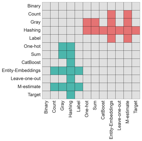
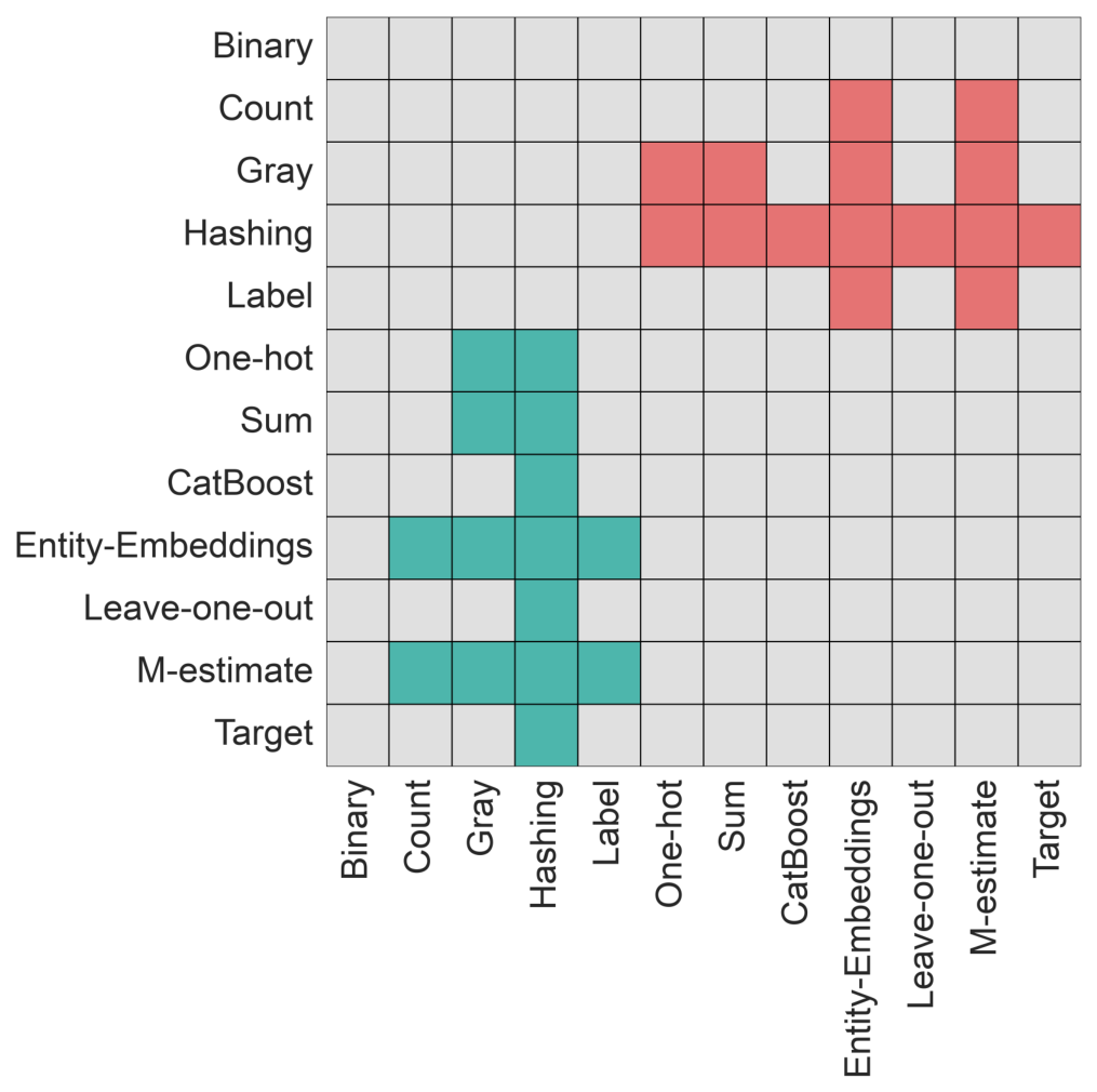
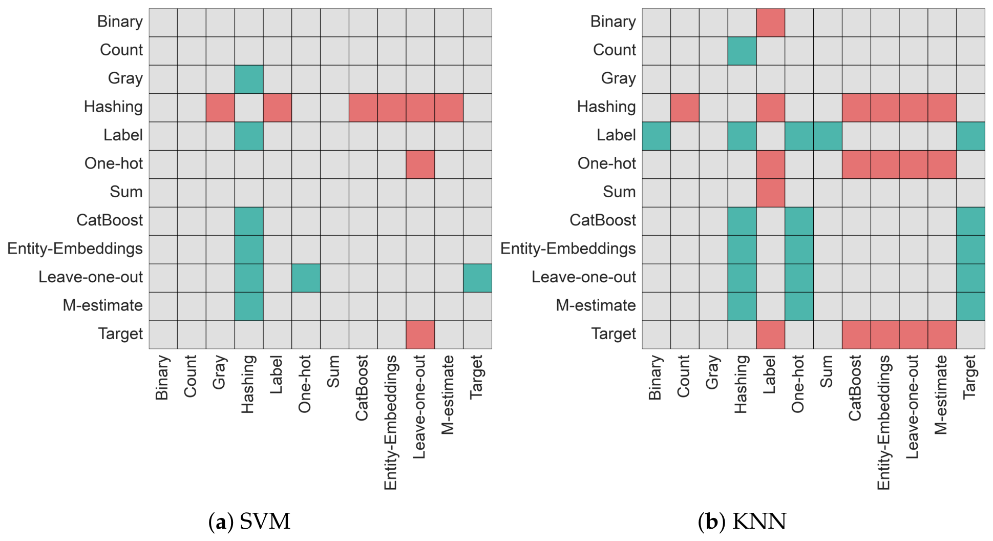
To answer the first two questions, the Friedman test [31,32] was used in an omnibus fashion to check for a statistically significant difference in complexity values at . If a significant difference was detected, a post-hoc Holm [32] was performed, also with . These results were visualized using a heatmap. Gray squares denote no statistical difference between encoders. Colored squares signify statistical significance. Green indicates that the encoder group on the y-axis has a lower median value compared to the group on the x-axis. Likewise, red indicates that the encoder group on the y-axis has a higher median value compared to the group on the x-axis.
The third question was answered in the same fashion as the first two questions: by computing the Friedman test in an omnibus fashion to check for a statistically significant difference in classifier performance between encoders.
Lastly, the fourth question was answered by computing the Spearman rank correlation [33] between the complexity measure values of the encoded datasets and the macro- scores of a classifier. This comparison was repeated for each complexity measure and classifier, as well as each complexity measure and the pooled scores of all classifiers.
5. Results
This section presents the results of the four experiments outlined in Section 4. The source code for the experiments and results have been made available on GitHub (https://github.com/KyleErwin/nominal-complexity, accessed on 21 September 2026). Section 5.1 presents the results of the first experiment, which investigates which categorical encoder for nominal data minimizes the values across each group of complexity characteristics. The second experiment, discussed in Section 5.2, investigated which encoder minimizes the complexity characteristic values for specific types of classification problems. Section 5.3 examines the relationship between choice of encoder and classifier performance (the third experiment), and how the complexity of the encoded datasets relates to classifier performance (the fourth experiment). Practical recommendations based on the results are given in Section 5.4.
5.1. Complexity Measures
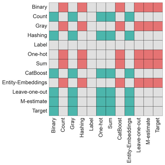
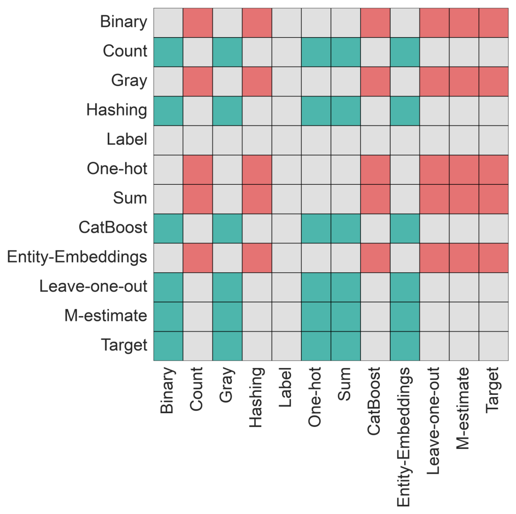
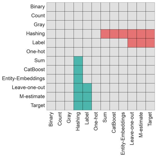
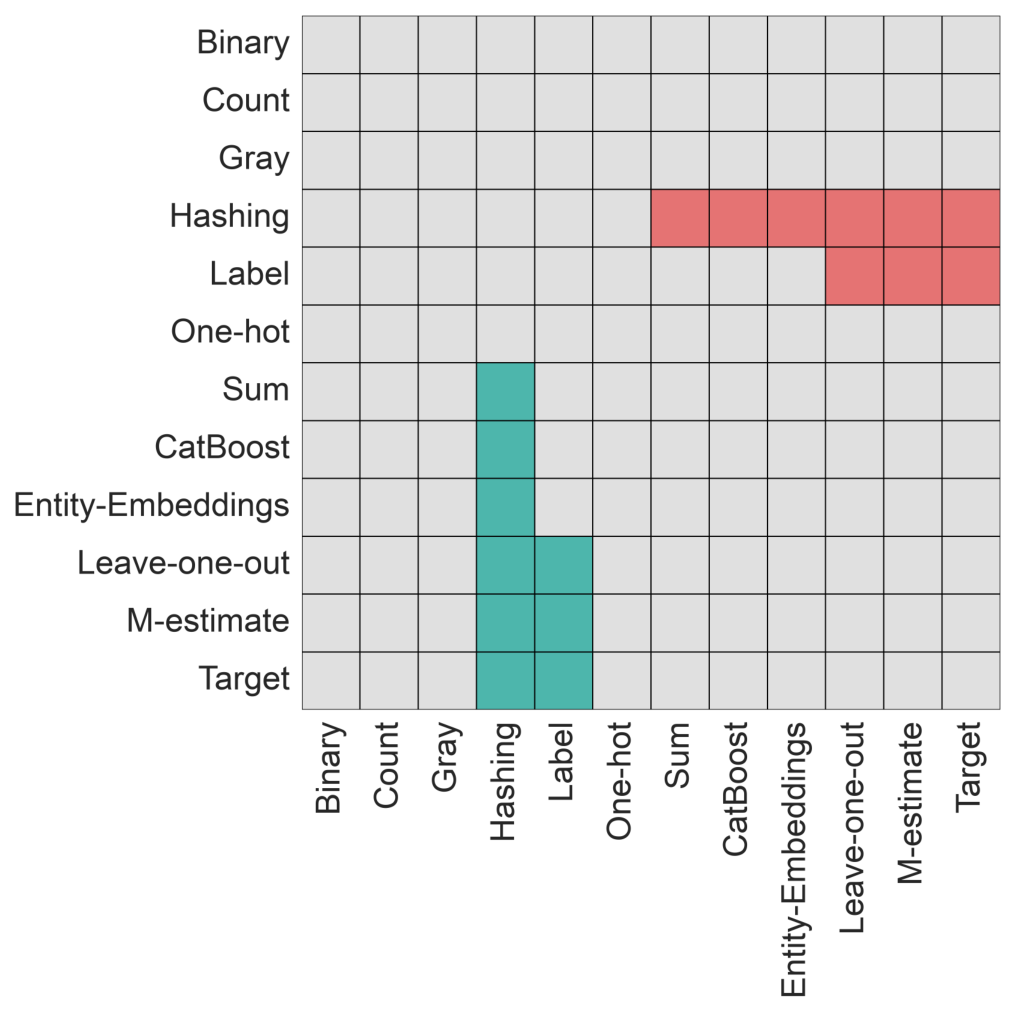
Figure 1 presents the results of the Holm post-hoc analysis of the encoders concerning dimensionality measures. The count, hashing, leave-one-out, CatBoost, target, and M-estimate encoders each resulted in datasets with statistically significantly lower dimensionality values than five other encoders, and were statistically indistinguishable from one another. In contrast, the binary, gray, one-hot, sum, label, and entity-embedding encoders were not statistically significantly better than any other encoder. This makes sense, since the count and hashing encoders do not create new features, and hashing in particular is useful for reducing the dimensionality of categorical features, whereas one-hot, sum, and entity-embeddings expand each categorical feature into multiple columns.
Figure 1.
Holm post-hoc analysis of the dimensionality measures (D1–D3) across the twelve categorical encoders. Each cell compares the encoder on the vertical axis with the encoder on the horizontal axis under a Holm post-hoc test at , applied after an omnibus Friedman test. Green indicates that the encoder on the vertical axis has the significantly lower median value of the two and is therefore preferred; red indicates that it has the significantly higher median value; grey indicates that the difference between the two encoders is not statistically significant.
The entity-embedding encoder was statistically significantly better than all eleven other encoders at producing datasets that minimize feature-based complexity measures (refer to Figure 2). In other words, this encoder encodes nominal features into numerical features that are more useful in discriminating instances of different classes than any of the other encoders. The one-hot, sum encoders and the four supervised encoders were each significantly better than the count, gray, hashing and label encoders. Additionally, the one-hot and sum encoders were also significantly better than the binary encoder.
Figure 2.
Holm post-hoc analysis of the feature-based measures (F1, F1v, F2–F5) across the twelve categorical encoders. Each cell compares the encoder on the vertical axis with the encoder on the horizontal axis under a Holm post-hoc test at , applied after an omnibus Friedman test. Green indicates that the encoder on the vertical axis has the significantly lower median value of the two and is therefore preferred; red indicates that it has the significantly higher median value; grey indicates that the difference between the two encoders is not statistically significant.
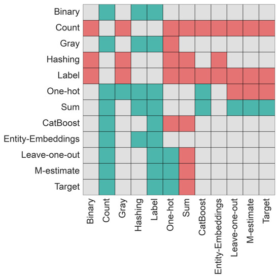
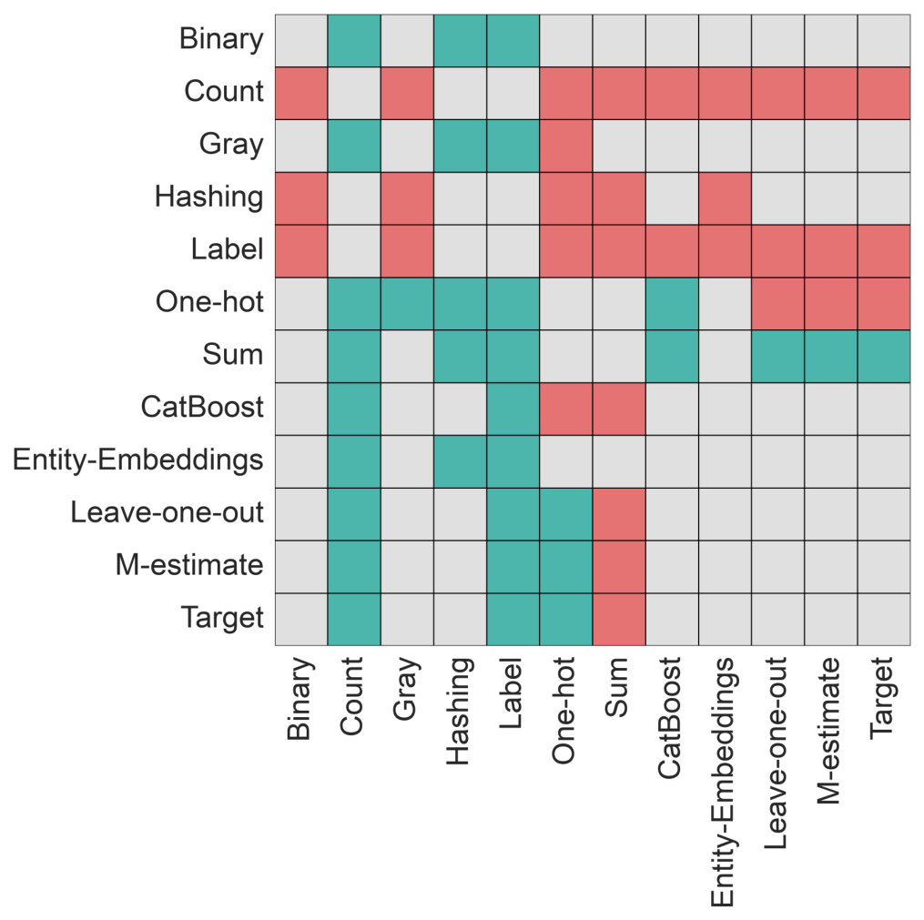
Figure 3 shows the results of the statistical significance tests for the linearity measures. The sum encoder was statistically significantly better than seven other encoders, which indicates that it produced the most linearly separable datasets. The one-hot encoder was significantly better than five other encoders. This result makes sense since the one-hot encoder expands the number of features by creating new binary features of the categorical values; thus creating more opportunity for linearly separable features. The label encoder resulted in statistically significantly higher values for the linearity measures.
Figure 3.
Holm post-hoc analysis of the linearity measures (L1–L3) across the twelve categorical encoders. Each cell compares the encoder on the vertical axis with the encoder on the horizontal axis under a Holm post-hoc test at , applied after an omnibus Friedman test. Green indicates that the encoder on the vertical axis has the significantly lower median value of the two and is therefore preferred; red indicates that it has the significantly higher median value; grey indicates that the difference between the two encoders is not statistically significant.
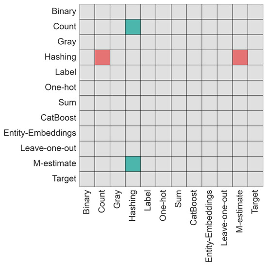
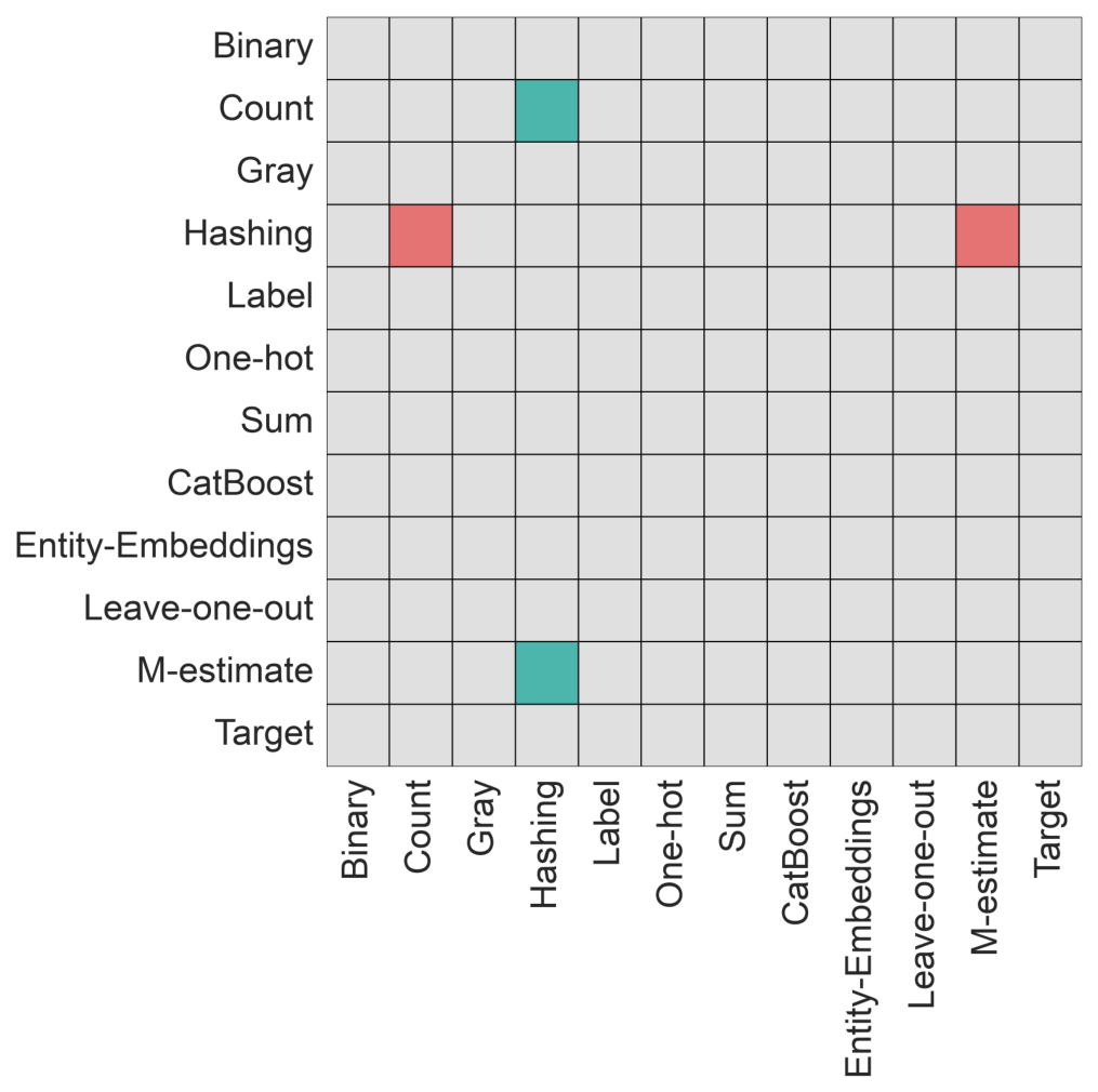
The statistical rankings for the neighborhood complexity measures (Figure 4) show that encoders were statistically indistinguishable from one another, with the exception of two cases. The count and M-estimate encoders were significantly better than the hashing encoder. Neighborhood complexity measures estimate the complexity of the decision boundary by analyzing local neighborhoods of instances. The results therefore suggest that the choice of encoder has no effect on the decision boundaries between classes and how much the classes overlap from a neighborhood complexity perspective.
Figure 4.
Holm post-hoc analysis of the neighborhood measures (N1–N6) across the twelve categorical encoders. Each cell compares the encoder on the vertical axis with the encoder on the horizontal axis under a Holm post-hoc test at , applied after an omnibus Friedman test. Green indicates that the encoder on the vertical axis has the significantly lower median value of the two and is therefore preferred; red indicates that it has the significantly higher median value; grey indicates that the difference between the two encoders is not statistically significant.
Lastly, Figure 5 shows the results for the structural complexity measures.
Figure 5.
Holm post-hoc analysis of the structural measures (G1–G3) across the twelve categorical encoders. Each cell compares the encoder on the vertical axis with the encoder on the horizontal axis under a Holm post-hoc test at , applied after an omnibus Friedman test. Green indicates that the encoder on the vertical axis has the significantly lower median value of the two and is therefore preferred; red indicates that it has the significantly higher median value; grey indicates that the difference between the two encoders is not statistically significant.
The M-estimate encoder performed statistically significantly better than four other encoders (i.e., binary, gray, hashing and label), and worse than one encoder (i.e., one-hot). The leave-one-out and CatBoost encoders were significantly better than three other encoders and the target encoder was significantly better than two other encoders. These results indicate that the supervised encoders tend to produce datasets that are simpler when represented as graphs. However, many comparisons between encoders were not statistically significant, suggesting that in general the graphs of the encoded datasets are of similar complexity.
5.2. Classification Problem Types
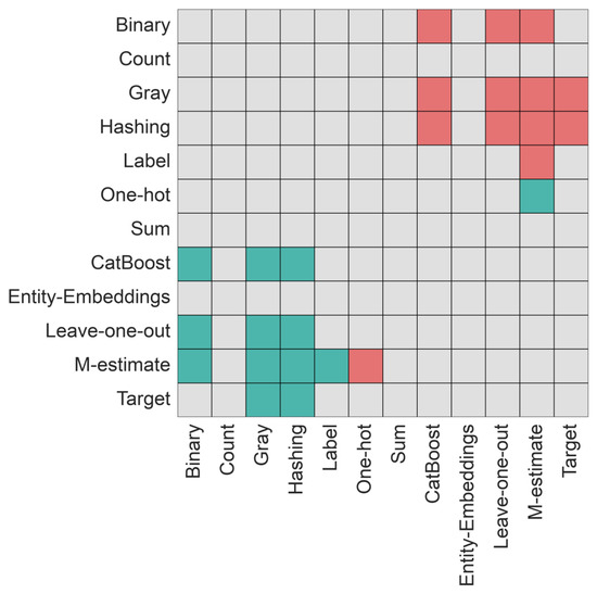
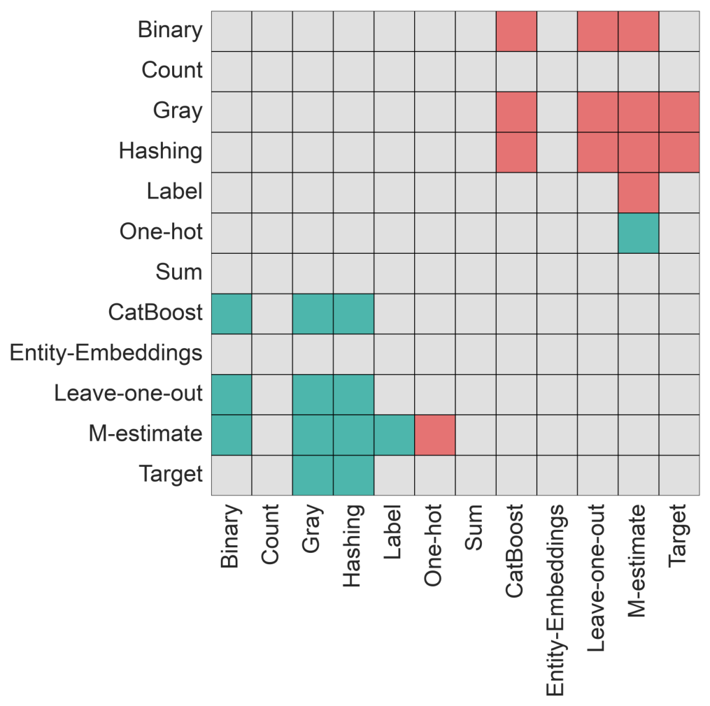
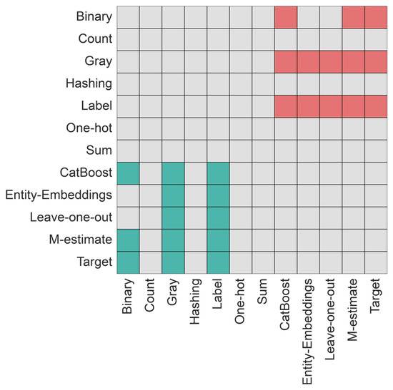
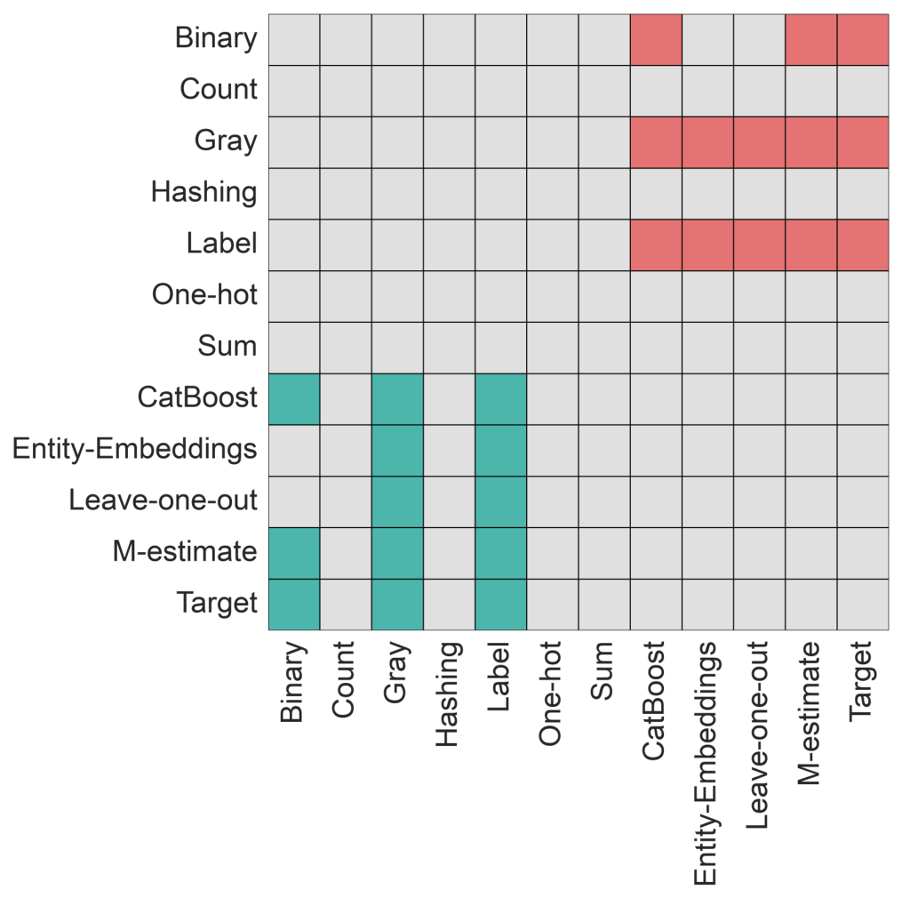
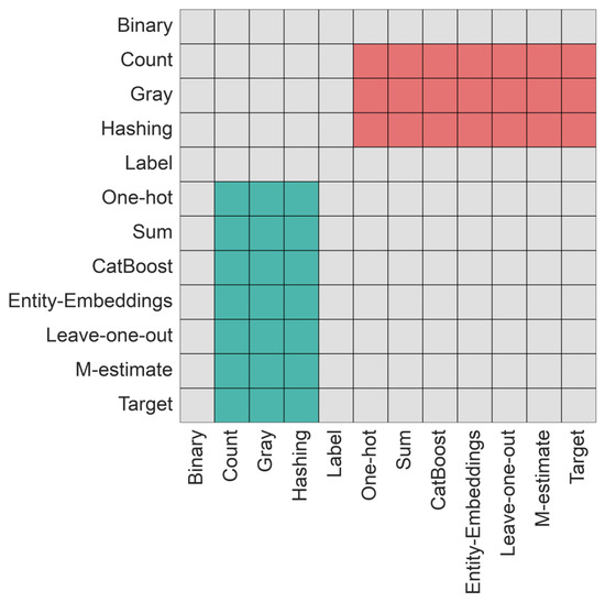
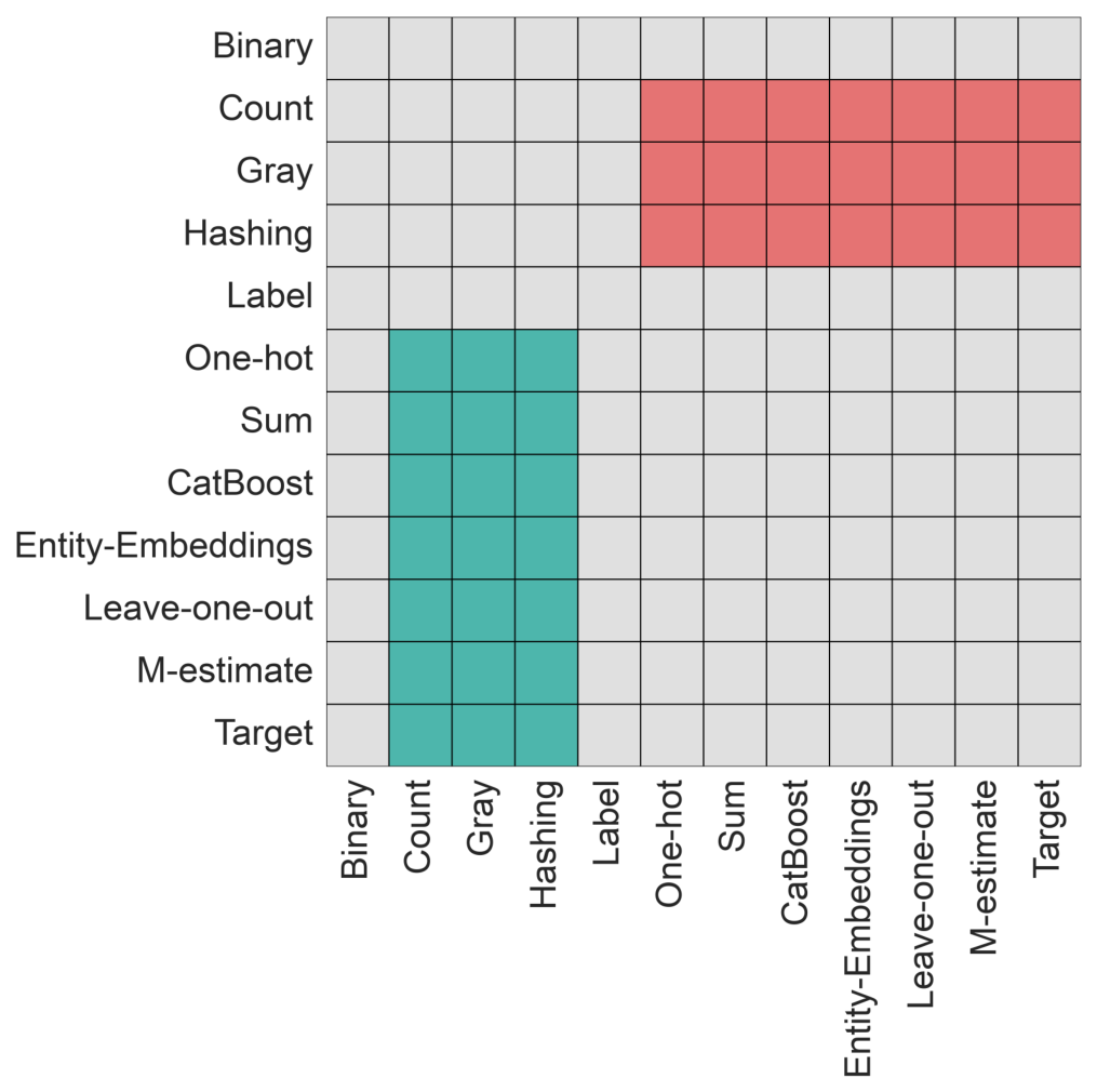
Figure 6, Figure 7, Figure 8 and Figure 9 show the results for the four problem types. The figures show that, in general, there is a slight advantage to using any of the supervised encoders and a disadvantage to using the count, gray, hashing and label encoders. However, in most cases there is no meaningful statistical difference in the resulting complexity values. One result worth noting is that the complexity values of binary-class classification problems with mixed features (refer to Figure 8) encoded using either the count, gray or hashing encoders were statistically significantly larger than than seven other encoders.
Figure 6.
Holm post-hoc analysis of all twenty-one complexity measures, restricted to the binary-class datasets with only nominal features. Each cell compares the encoder on the vertical axis with the encoder on the horizontal axis under a Holm post-hoc test at , applied after an omnibus Friedman test. Green indicates that the encoder on the vertical axis has the significantly lower median value of the two and is therefore preferred; red indicates that it has the significantly higher median value; grey indicates that the difference between the two encoders is not statistically significant.
Figure 7.
Holm post-hoc analysis of all twenty-one complexity measures, restricted to the multi-class datasets with only nominal features. Each cell compares the encoder on the vertical axis with the encoder on the horizontal axis under a Holm post-hoc test at , applied after an omnibus Friedman test. Green indicates that the encoder on the vertical axis has the significantly lower median value of the two and is therefore preferred; red indicates that it has the significantly higher median value; grey indicates that the difference between the two encoders is not statistically significant.
Figure 8.
Holm post-hoc analysis of all twenty-one complexity measures, restricted to the binary-class datasets with both nominal and numeric features. Each cell compares the encoder on the vertical axis with the encoder on the horizontal axis under a Holm post-hoc test at , applied after an omnibus Friedman test. Green indicates that the encoder on the vertical axis has the significantly lower median value of the two and is therefore preferred; red indicates that it has the significantly higher median value; grey indicates that the difference between the two encoders is not statistically significant.
Figure 9.
Holm post-hoc analysis of all twenty-one complexity measures, restricted to the multi-class datasets with both nominal and numeric features. Each cell compares the encoder on the vertical axis with the encoder on the horizontal axis under a Holm post-hoc test at , applied after an omnibus Friedman test. Green indicates that the encoder on the vertical axis has the significantly lower median value of the two and is therefore preferred; red indicates that it has the significantly higher median value; grey indicates that the difference between the two encoders is not statistically significant.
5.3. Classifier Performance
The omnibus Friedman test found that the choice of encoder has a statistically significant impact on the performance of the SVM () and of the KNN classifier () but not on the performance of the random forest ().
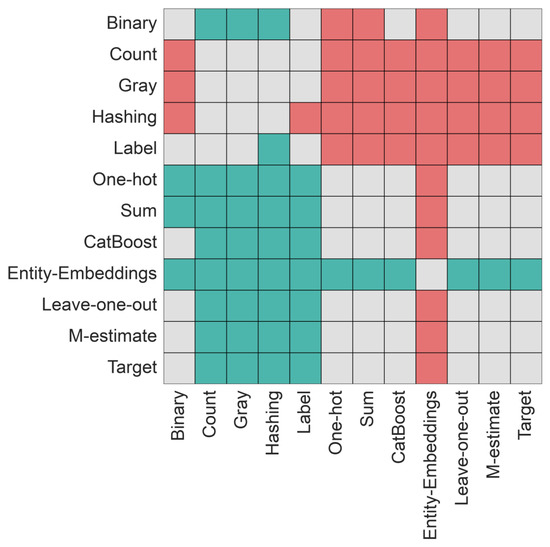
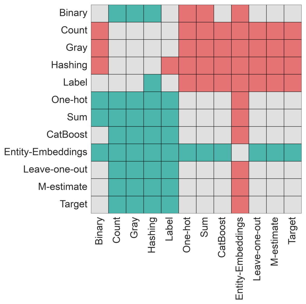
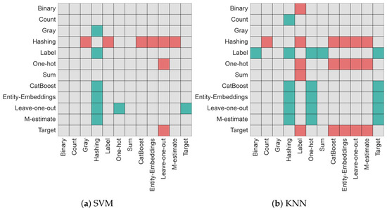
Figure 10a shows that the hashing encoder resulted in statistically significantly worse performance for the SVM classifier than the gray, label, leave-one-out, CatBoost, target and M-estimate encoders. The target encoder resulted in statistically significantly better performance than the one-hot and entity-embedding encoders. For the KNN classifier (Figure 10b), the supervised encoders (with the exception of the target encoder) and the label encoder led to statistically significantly better performance than the hashing, one-hot and entity-embedding encoders, and the label encoder was also statistically significantly better than the binary and sum encoders.
Figure 10.
Holm post-hoc analysis of the macro- scores across the twelve categorical encoders for the SVM and KNN classifiers. Each cell compares the encoder on the vertical axis with the encoder on the horizontal axis under a Holm post-hoc test at , applied after an omnibus Friedman test. Green indicates that the encoder on the vertical axis has the significantly lower median value of the two and is therefore preferred; red indicates that it has the significantly higher median value; grey indicates that the difference between the two encoders is not statistically significant.
The hashing encoder resulted in the lowest median macro- of all twelve encoders for every classifier, whereas the target encoder resulted in the highest median for the random forest and the KNN classifier, and the binary encoder was the highest for the SVM. These results are tabulated in Appendix C.
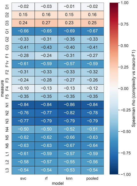
Figure 11 shows the results of the Spearman rank correlation between the macro- scores of the classifiers and the complexity values of the datasets. The neighborhood complexity measures correlate strongly in a negative direction, which means that lower neighborhood complexity is associated with a higher macro-. The correlation values between the pooled scores and the N1, N2 and N3 measures are , and respectively. There are also slightly weaker correlations () between the pooled scores and the remaining neighborhood measures, the linearity measures, the G1 measure and the F1v measure. The remaining feature-based complexity measures and structural measures are weakly correlated () with classifier performance in a negative direction, with the exception of the F4 measure (). The D1 measure, which is the average number of features per instance, is not correlated with classifier performance. Lastly, the remaining two dimensionality measures, D2 () and D3 (), are weakly positively correlated with classifier performance. These correlation values suggest that datasets with more principal components tend to result in slightly higher classifier performance.
Figure 11.
Spearman rank correlation between each complexity measure and macro-, per classifier and pooled. Rows are the twenty-one complexity measures and columns are the three classifiers, with the rightmost column pooling the macro- scores of all three. Each cell is the Spearman rank correlation coefficient computed over all (dataset, encoder) pairs for that classifier.
5.4. Discussion
Two important results of the paper are that the choice of encoder has an effect on the performance of SVM and KNN and that the complexity of an encoded dataset is informative about the performance that can be attained on it. A practitioner can use the first result to base his decision on which encoder to use or avoid when encoding data for an SVM or KNN classifier. That is, in general, the hashing encoder is a poor choice of encoder when compared to other encoders for maximizing SVM and KNN classifier performance. Additionally, the one-hot and target encoders, in general, should be avoided for the KNN classifier.
A practitioner can use the second result to make feature-engineering decisions based on what minimizes the strongly correlated complexity measures. For example, the N1 measure, which computes the fraction of borderline points, is strongly negatively correlated () with macro- scores. The other neighborhood complexity measures, as well as the structural and linearity complexity measures, are also correlated with classification performance.
However, the Holm post-hoc analysis of the structural and linearity complexity measures showed that there was no clear best encoder but rather which encoders performed the worst (count, gray and hashing). Similarly, the encoders were, in all cases but two, statistically indistinguishable from each other with regard to neighborhood complexity values. This means that encoders alone have no impact on minimizing the most informative complexity measures for classifier performance. Future work should explore whether there are data pipelines for minimizing said informative complexity measures.
6. Conclusions
Categorical data is a fundamental type of data that is commonly seen in real-world datasets across various problem domains. However, machine learning algorithms primarily operate on numerical data, making it essential for some algorithms to convert categorical data into a numerical format. Categorical encoding strategies are methods of converting categorical data into a numerical format that can be used in machine learning algorithms. Since each encoder has its unique characteristics, it is reasonable to assume that the properties of a dataset would vary when encoded using different categorical encoders.
This paper investigated which encoder produces the simplest encoded datasets. Twelve categorical encoders for nominal data were used to encode 43 open-source datasets, resulting in twelve variations of each dataset. A variety of complexity characteristics were then collected on the resulting encoded datasets. An omnibus Friedman test with post-hoc Holm analysis () was used to test for any statistically meaningful differences in the complexity characteristics of the encoded datasets [33]. The first experiment aimed to determine which encoder produces the simplest datasets with respect to each group of complexity characteristics, and the second experiment investigated which encoder produces the simplest datasets for differing types of classification problems.
The results showed that no single encoder produces the least complex datasets across all complexity measures. However, the supervised encoders studied (i.e., leave-one-out, CatBoost, target, M-estimate and entity-embedding) produced statistically significantly lower feature-based complexity values and structural complexity values, with the entity-embedding encoder outperforming all other encoders with regard to the feature-based measures. It was also found that, in general, there was a slight advantage to using any of the supervised encoders for the classification problem types considered. The paper showed that the choice of encoder has a statistically significant effect on the support vector machine classifier and on the k-nearest neighbor classifier but not on the random forest. Furthermore, it was found that the neighborhood, structural, and linearity complexity values of the encoded datasets correlate with classification performance. Overall, the results support the idea that there is a relationship between classifier performance and complexity measures and can serve as the foundation for future investigations into data transformation pipelines and their impact on complexity and performance.
7. Future Work
Future work should investigate whether there is a data pipeline that includes a series of data transformations that results in both statistically significantly better classifier performance and statistically significantly lower complexity values.
Author Contributions
Conceptualization, K.E. and A.E.; methodology, K.E. and A.E.; software, A.E.; validation, K.E.; formal analysis, K.E.; investigation, K.E. and A.E.; resources, A.E.; data curation, A.E.; writing—original draft preparation, K.E.; writing—review and editing, K.E. and A.E.; visualization, K.E.; supervision, A.E.; project administration, K.E. and A.E. All authors have read and agreed to the published version of the manuscript.
Funding
This research received no external funding.
Institutional Review Board Statement
Not applicable.
Informed Consent Statement
Not applicable.
Data Availability Statement
The source code and data for the experiments have been made available at https://github.com/KyleErwin/nominal-complexity (accessed on 21 September 2026).
Conflicts of Interest
Author Kyle Erwin is employed by the company IBM. The remaining author declares that the research was conducted in the absence of any commercial or financial relationships that could be construed as a potential conflict of interest.
Abbreviations
The following abbreviations are used in this manuscript:
| 1NN | 1-nearest neighbor |
| CatBoost | Categorical boosting |
| FNN | Feed-forward neural network |
| KNN | K-nearest neighbor |
| MST | Minimum spanning tree |
| PCA | Principal component analysis |
| PyMFE | Python library meta-feature extractor |
| RF | Random forest |
| SVM | Support vector machine |
Appendix A. OpenML Datasets
Table A1.
Dataset details.
Appendix B. Encoder Parameter Values
Table A2.
Parameter values for the eleven encoders are from category_encoders.
Appendix C. Classifier Performance per Dataset
Table A3.
Mean ± standard deviation of the macro- score across the twelve encoders, per dataset and classifier.
References
- Hancock, J.T.; Khoshgoftaar, T.M. Survey on Categorical Data for Neural Networks. J. Big Data 2020, 7, 28. [Google Scholar] [CrossRef] [Scilit]
- Lorena, A.C.; Garcia, L.P.F.; Lehmann, J.; Souto, M.C.P.; Ho, T.K. How Complex Is Your Classification Problem? A Survey on Measuring Classification Complexity. ACM Comput. Surv. 2019, 52, 1–34. [Google Scholar] [CrossRef] [Scilit]
- Lorena, A.C.; Maciel, A.I.; de Miranda, P.B.C.; Costa, I.G.; Prudêncio, R.B.C. Data complexity meta-features for regression problems. Mach. Learn. 2018, 107, 209–246. [Google Scholar] [CrossRef] [Scilit]
- Simonoff, J.S. Analyzing Categorical Data; Springer Texts in Statistics; Springer: New York, NY, USA, 2003. [Google Scholar] [CrossRef] [Scilit]
- Zheng, A.; Casari, A. Feature Engineering for Machine Learning: Principles and Techniques for Data Scientists; O’Reilly Media, Inc.: Sebastopol, CA, USA, 2018. [Google Scholar]
- Weinberger, K.; Dasgupta, A.; Langford, J.; Smola, A.; Attenberg, J. Feature Hashing for Large Scale Multitask Learning. In Proceedings of the 26th Annual International Conference on Machine Learning; Association for Computing Machinery: New York, NY, USA, 2009; pp. 1113–1120. [Google Scholar] [CrossRef] [Scilit]
- Prokhorenkova, L.; Gusev, G.; Vorobev, A.; Dorogush, A.V.; Gulin, A. CatBoost: Unbiased boosting with categorical features. In Advances in Neural Information Processing Systems; Curran Associates, Inc.: Red Hook, NY, USA, 2018; Volume 31. [Google Scholar]
- Guo, C.; Berkhahn, F. Entity embeddings of categorical variables. arXiv 2016, arXiv:1604.06737. [Google Scholar]
- McGinnis, W. Leave One Out—Category Encoders 2.6.3 Documentation. Available online: https://contrib.scikit-learn.org/category_encoders/leaveoneout.html (accessed on 21 September 2026).
- Micci-Barreca, D. A preprocessing scheme for high-cardinality categorical attributes in classification and prediction problems. ACM SIGKDD Explor. Newsl. 2001, 3, 27–32. [Google Scholar] [CrossRef] [Scilit]
- Basu, M.; Ho, T.K. Data Complexity in Pattern Recognition; Springer Science & Business Media: Berlin/Heidelberg, Germany, 2006. [Google Scholar]
- Lorena, A.C.; Costa, I.G.; Spolaôr, N.; de Souto, M.C.P. Analysis of Complexity Indices for Classification Problems: Cancer Gene Expression Data. Neurocomputing 2012, 75, 33–42. [Google Scholar] [CrossRef] [Scilit]
- Okimoto, L.C.; Savii, R.M.; Lorena, A.C. Complexity Measures Effectiveness in Feature Selection. In Proceedings of the Brazilian Conference on Intelligent Systems; IEEE: Piscataway, NJ, USA, 2017; pp. 91–96. [Google Scholar]
- Ho, T.K.; Basu, M. Complexity measures of supervised classification problems. IEEE Trans. Pattern Anal. Mach. Intell. 2002, 24, 289–300. [Google Scholar] [CrossRef] [Scilit]
- Mollineda, R.A.; Sánchez, J.S.; Sotoca, J.M. Data characterization for effective prototype selection. In Proceedings of the Second Iberian conference on Pattern Recognition and Image Analysis, Part II; Springer: Berlin/Heidelberg, Germany, 2005; pp. 27–34. [Google Scholar]
- Orriols-Puig, A.; Macià, N.; Ho, T. DCoL: Data Complexity Library in C++ (Documentation); Technical Report; La Salle–Universitat Ramon Llull: Barcelona, Spain, 2010. [Google Scholar]
- Malina, W. Two-parameter Fisher criterion. IEEE Trans. Syst. Man Cybern. Part B (Cybern.) 2001, 31, 629–636. [Google Scholar] [CrossRef] [Scilit] [PubMed]
- Erwin, K.H.; Engelbrecht, A.P. Feature-Based Complexity Measure for Multinomial Classification Datasets. Entropy 2023, 25, 1000. [Google Scholar] [CrossRef] [Scilit] [PubMed]
- Cristianini, N.; Shawe-Taylor, J. An Introduction to Support Vector Machines and Other Kernel-Based Learning Methods; Cambridge University Press: Cambridge, UK, 2000. [Google Scholar] [CrossRef] [Scilit]
- Hoekstra, A.; Duin, R.P.W. On the nonlinearity of pattern classifiers. In Proceedings of the 13th International Conference on Pattern Recognition; IEEE: Piscataway, NJ, USA, 1996; pp. 271–275. [Google Scholar] [CrossRef] [Scilit]
- Pettie, S.; Ramachandran, V. An Optimal Minimum Spanning Tree Algorithm. J. ACM 2002, 49, 16–34. [Google Scholar] [CrossRef] [Scilit]
- Garcia, L.P.F.; de Carvalho, A.C.P.L.F.; Lorena, A.C. Effect of Label Noise in the Complexity of Classification Problems. Neurocomputing 2015, 160, 108–119. [Google Scholar] [CrossRef] [Scilit]
- Leyva, E.; González, A.; Pérez, R. A Set of Complexity Measures Designed for Applying Meta-Learning to Instance Selection. IEEE Trans. Knowl. Data Eng. 2015, 27, 354–367. [Google Scholar] [CrossRef] [Scilit]
- Gower, J.C. A General Coefficient of Similarity and Some of Its Properties. Biometrics 1971, 27, 857–871. [Google Scholar] [CrossRef] [Scilit]
- Morais, G.; Prati, R. Complex Network Measures for Data Set Characterization. In Proceedings of the Brazilian Conference on Intelligent Systems, BRACIS 2013; IEEE: Piscataway, NJ, USA, 2013; pp. 12–18. [Google Scholar] [CrossRef] [Scilit]
- Alcobaça, E.; Siqueira, F.; Rivolli, A.; Garcia, L.P.F.; Oliva, J.T.; de Carvalho, A.C.P.L.F. MFE: Towards Reproducible Meta-Feature Extraction. J. Mach. Learn. Res. 2020, 21, 1–5. [Google Scholar]
- Cover, T.; Hart, P. Nearest Neighbor Pattern Classification. IEEE Trans. Inf. Theory 1967, 13, 21–27. [Google Scholar] [CrossRef] [Scilit]
- Cortes, C.; Vapnik, V. Support-Vector Networks. Mach. Learn. 1995, 20, 273–297. [Google Scholar] [CrossRef] [Scilit]
- Breiman, L. Random Forests. Mach. Learn. 2001, 45, 5–32. [Google Scholar] [CrossRef] [Scilit]
- Pedregosa, F.; Varoquaux, G.; Gramfort, A.; Michel, V.; Thirion, B.; Grisel, O.; Blondel, M.; Prettenhofer, P.; Weiss, R.; Dubourg, V.; et al. Scikit-learn: Machine Learning in Python. J. Mach. Learn. Res. 2011, 12, 2825–2830. [Google Scholar]
- Friedman, M. The Use of Ranks to Avoid the Assumption of Normality Implicit in the Analysis of Variance. J. Am. Stat. Assoc. 1937, 32, 675–701. [Google Scholar] [CrossRef]
- Demšar, J. Statistical Comparisons of Classifiers over Multiple Data Sets. J. Mach. Learn. Res. 2006, 7, 1–30. Available online: http://jmlr.org/papers/v7/demsar06a.html (accessed on 21 September 2026).
- Sheskin, D.J. Handbook of Parametric and Nonparametric Statistical Procedures; Chapman and Hall/CRC: Boca Raton, FL, USA, 2011. [Google Scholar]

Disclaimer/Publisher’s Note: The statements, opinions and data contained in all publications are solely those of the individual author(s) and contributor(s) and not of MDPI and/or the editor(s). MDPI and/or the editor(s) disclaim responsibility for any injury to people or property resulting from any ideas, methods, instructions or products referred to in the content. |
© 2026 by the authors. Licensee MDPI, Basel, Switzerland. This article is an open access article distributed under the terms and conditions of the Creative Commons Attribution (CC BY) license.