Toward Explainable AI for Acute Kidney Injury Prediction in the ICU: Transparent Development, Internal Validation, and Robustness Auditing of Machine Learning Models

Abstract

Background/Objectives: Acute kidney injury (AKI) is common in critical care, yet predictive artificial intelligence studies often differ in outcome definitions, validation, calibration, and interpretability. We developed and internally validated machine learning models for newly observed serum-creatinine-defined AKI after a fixed 24 h ICU landmark and then audited how stable the selected model was to clinically important observation and timing choices. Methods: Using MIMIC-IV v3.1, we retained one first ICU stay per adult patient, required adequate pre-landmark creatinine observation, excluded coded end-stage kidney disease, documented dialysis before the landmark, and observed AKI by the landmark. The outcome was a new creatinine rise within the next 48 h using KDIGO-aligned creatinine change thresholds, with follow-up truncated at ICU exit, hospital discharge, or death. The ascertainable cohort (n = 15,231) was split 60%/15%/10%/15% into training, calibration, validation, and test sets. Logistic regression, random forests, and histogram gradient boosting were calibrated with a separate calibration set; thresholds were fixed on validation data to target at least 80% sensitivity. The test set was evaluated once. A later post hoc audit reused frozen test risks without retraining. Results: Histogram gradient boosting was selected by validation average precision. In 2286 test patients (664 events; 29.0%), AUROC was 0.726 (95% CI, 0.701–0.749), average precision 0.523 (0.478–0.565), and Brier score 0.179 (0.171–0.187). At the fixed threshold, sensitivity was 78.5%, specificity 52.2%, positive predictive value 40.2%, and false alerts 33.9 per 100 patients. Mean predicted risk was 0.290 versus an observed event fraction of 0.290; calibration intercept and slope were 0.023 and 1.022. The AUROC difference versus full logistic regression was +0.0197 (95% CI, 0.00235–0.03571). Frozen-model sensitivity analyses produced AUROCs from 0.697 to 0.733 in most observation and measurement subsets. However, 15,900 otherwise eligible patients had indeterminate outcomes and showed substantially shorter follow-up and fewer post-landmark creatinine measurements. Conclusions: The selected model showed moderate discrimination and close aggregate calibration under internal validation. Discrimination was similar across several post hoc subsets, although calibration and threshold-based performance changed under stricter observation rules. The main limitation was observation-dependent outcome ascertainment. This work supports transparent model auditing as part of trustworthy AI evaluation, but it does not provide external validation, patient-level explanation validation, or evidence of clinical benefit. Multicenter temporal validation and prospectively defined observation rules are needed before clinical use.

1. Introduction

Acute kidney injury (AKI) is a heterogeneous syndrome marked by a rapid decline in kidney function and is associated with short- and long-term complications [1]. The Kidney Disease: Improving Global Outcomes (KDIGO) framework defines AKI using changes in serum creatinine and urine output, including an increase in creatinine of at least 0.3 mg/dL within 48 h or at least 1.5 times baseline within seven days [2]. In the multinational AKI-EPI study, AKI occurred in more than half of ICU patients when KDIGO criteria were applied, and increasing severity was associated with worse outcomes [3]. These features make AKI a frequent target for risk prediction in critical care.

A large body of literature has explored electronic health record (EHR) models for AKI prediction. ICU and hospital studies have reported useful discrimination using regression, random forests, gradient boosting, and deep learning [4,5,6,7,8]. Yet the apparent performance of a model depends strongly on the population, prediction time, outcome definition, observation process, and validation design. Systematic reviews have repeatedly found high risk of bias, limited external validation, inconsistent calibration reporting, and wide variation in clinical applicability [9,10,11,12]. A 2025 review focused on ICU AI models found that only a minority of included studies used external validation and highlighted interpretability and clinical integration as continuing gaps [11]. Model transparency and interpretability add another challenge. Recent AKI studies have begun to use feature-attribution methods such as SHAP to identify influential variables [13], and a 2026 scoping review described growing interest in explainable AKI prediction while noting that clinical validation of explanations remains limited [14]. In high-stakes settings, however, an explanation graphic does not by itself establish that a model is safe, clinically meaningful, or transportable. Methodological work has therefore argued for interpretable comparators, careful evaluation of black-box models, and explicit attention to what an explanation can and cannot establish [15,16,17]. For this reason, we use a deliberately narrow meaning of transparency. We do not claim patient-level mechanistic explanations. Instead, we make the data timing, cohort construction, predictor definitions, model comparison, calibration, threshold choice, decision analysis, and post hoc robustness check visible and reproducible. This approach is consistent with the reporting goals of TRIPOD+AI, the risk-of-bias focus of PROBAST+AI, and the transparency principles in MI-CLAIM [18,19,20].

The objective was to develop and internally validate machine learning models for newly observed serum-creatinine-defined AKI after a 24 h ICU landmark using routinely available EHR data from MIMIC-IV, then audit the selected model without retraining. We asked four practical questions: (1) whether a nonlinear model offered meaningful improvement over a full logistic model; (2) whether predicted probabilities were calibrated in the held-out test set; (3) whether performance remained stable under alternative observation and timing restrictions; and (4) how patients with ascertainable outcomes differed from otherwise eligible patients whose outcomes were indeterminate.

2. Materials and Methods

2.1. Study Design and Reporting

This was a retrospective prognostic model development and internal-validation study using a fixed 24 h ICU landmark. The primary analysis protocol, model set, split, model-selection rule, calibration procedure, threshold procedure, and test evaluation were frozen before scoring the test set. A separate robustness audit was designed after the primary test results were available. The audit therefore remains explicitly post hoc and exploratory. Reporting was organized with TRIPOD+AI and MI-CLAIM principles in mind [18,20], while PROBAST+AI informed the emphasis on validation, outcome definition, analysis, and applicability [19].

2.2. Data Source and Ethical Context

Data came from MIMIC-IV v3.1, a deidentified EHR resource derived from routine care at Beth Israel Deaconess Medical Center. MIMIC-IV v3.1 contains hospital and ICU data from 2008 through 2022, including laboratory measurements, diagnoses, procedures, orders, and treatments [21,22]. Version 3.1 was released through PhysioNet in October 2024 [22]. The source resource is shared with credentialed researchers under a data use agreement. The MIMIC-IV publication reports approval by the Beth Israel Deaconess Medical Center Institutional Review Board for sharing the deidentified research resource and a waiver of informed consent [21]. The analysis used the patients, admissions, ICU stays, diagnoses, laboratory events, prescriptions, provider order entry, and procedure-event tables. All patient-level processing remained within the permitted MIMIC environment; only aggregate outputs are reported here.

2.3. Population and Prediction Landmark

The unit of analysis was the first recorded ICU stay for each subject, selected before outcome filtering so that one patient contributed at most one row. Adults who were alive and still in the ICU 24 h after ICU admission were eligible for the prediction landmark. Ages at or above 90 years were top-coded to 90 because exact older ages are not recoverable from the deidentified data. We excluded patients with an index-admission code for end-stage renal disease (ICD-9 5856 or ICD-10 N186) and those with a documented dialysis procedure beginning by the 24 h landmark. We then required at least two distinct pre-landmark creatinine measurements with results available by the landmark, including at least one measurement during the first 24 ICU hours. Patients with an observed qualifying creatinine rise between ICU entry and the landmark were excluded. The intended target population was therefore adult ICU patients who were alive and still in the ICU at the 24 h landmark, satisfied these prespecified renal and creatinine-observation criteria, and had no qualifying creatinine rise observed between ICU entry and the landmark. However, inclusion in the final analytic cohort additionally required an ascertainable post-landmark outcome under the rules described in Section 2.4. Consequently, the predictive performance, calibration, and threshold-based operating characteristics reported in this study pertain to the outcome-ascertainable subset of this target population and should not be assumed to represent all patients who satisfied the pre-landmark eligibility criteria. Outcome ascertainability depended on post-landmark follow-up and creatinine measurement and therefore could not be determined from the pre-landmark eligibility criteria alone. These are retrospective cohort-definition rules rather than claims about what would have been known to a clinician in real time.

2.4. Outcome Definition and Outcome Ascertainment

The target outcome was a newly observed creatinine-defined qualifying rise after the 24 h ICU landmark. For each creatinine measurement, the algorithm evaluated eligible earlier creatinine measurements within the preceding 48 h for the absolute-change criterion and within the preceding seven days for the ratio criterion. When multiple eligible earlier creatinine measurements were available within a look-back window, the lowest eligible earlier value was used as the reference value, corresponding to the rolling-minimum implementation used in the analysis. A qualifying rise was defined as an increase in serum creatinine of at least 0.3 mg/dL relative to an eligible earlier value within 48 h or a ratio of at least 1.5 relative to an eligible earlier value within seven days, reflecting the serum-creatinine components of KDIGO [2]. Simultaneous measurements were collapsed to their median and were not permitted to serve as reference measurements for one another. This operational outcome was not equivalent to full KDIGO-defined incident AKI or AKI staging because it did not incorporate urine output, dialysis alone as an outcome, an outpatient historical creatinine baseline, or an inferred normal baseline. Baseline laboratory history was limited to the index hospitalization and began no earlier than seven days before ICU admission. These choices reduced assumptions about unobserved baseline kidney function but could miss qualifying creatinine changes when an appropriate earlier reference value was unavailable.

The maximum post-landmark observation window was 48 h; however, observation was truncated earlier at the first occurrence of ICU exit, hospital discharge, or death. Accordingly, the prediction target should be interpreted as a qualifying creatinine rise observed after the 24 h landmark and before the earlier of 48 h or observation termination, rather than as an unconditional 48 h AKI risk. A positive outcome required at least one qualifying post-landmark creatinine rise before the end of this patient-specific observation window. A negative outcome required at least one valid post-landmark creatinine measurement and required the final valid post-landmark measurement to occur within 12 h of the end of the observation window. Patients who met neither the positive nor the negative ascertainment rule were classified as indeterminate and were excluded from model development and primary performance evaluation. Because positive cases were not required to satisfy the same final-laboratory observation requirement as negative cases, outcome ascertainment depended on subsequent observation and measurement processes. Thus, the reported predictive performance and calibration apply to patients whose outcomes were ascertainable under these rules rather than to all patients meeting the pre-landmark eligibility criteria. This asymmetry in outcome ascertainment was a central focus of the subsequent post hoc audit. Operationally, the timing rules were applied in the following order: (1) predictor laboratory values were eligible only when both chart time and storage time were no later than the 24 h landmark; (2) the pre-landmark qualifying-rise exclusion used creatinine chart time from ICU admission through the landmark, including results stored after the landmark; (3) post-landmark qualifying rises were identified using creatinine chart time within the patient-specific observation window, including qualifying measurements whose results were stored after the observation endpoint; (4) negative-outcome ascertainment required the final valid post-landmark creatinine chart time to occur within 12 h of the observation endpoint; and (5) among positive cases, a qualifying result was flagged as late when its storage time was missing or when its earliest recorded storage time occurred after the patient-specific observation endpoint. Late qualifying results were retained in the primary chart-time-based outcome definition and were excluded only in the corresponding post hoc sensitivity analysis.

2.5. Predictors and Timing

Forty-six predictors were formed from information available by the 24 h landmark. Demographic and timing variables were age, recorded sex, hours from hospital admission to ICU admission, and an indicator for an intravenous vancomycin prescription linked to a provider-order-entry time by the landmark. The medication variable represented a time-confirmed prescription order, not administration, continued treatment, drug exposure, or a causal effect.

Laboratory predictors came from creatinine, blood urea nitrogen, sodium, potassium, bicarbonate, glucose, white blood cell count, hemoglobin, platelets, and albumin. For predictor construction, both chart time and storage time were required to be no later than the 24 h landmark so that laboratory results unavailable at prediction time were not used. For each laboratory family, first-24 h values were summarized using the last, minimum, maximum, and count. Creatinine additionally included the first value and the change from the first to the last eligible first-24 h measurement. When only one eligible creatinine measurement was available within the first 24 ICU hours, the first and last values were identical, and the creatinine-change variable was therefore 0 mg/dL. The use of both chart and storage timestamps was intended to prevent information leakage from results charted before the landmark but not yet available in the record at prediction time.

2.6. Data Splitting and Models

The final ascertainable cohort was randomly split, with outcome stratification and disjoint subjects, into training (60%), calibration (15%), model-selection validation (10%), and test (15%) partitions. The split was an internal random split; it was not temporal, internal–external, or external validation. Six candidates were evaluated: a prevalence-only reference; a full logistic regression model; a lean random forest using age, recorded sex, last creatinine, and the vancomycin-order indicator; a full random forest; a full random forest retrained without the vancomycin feature; and histogram gradient boosting. Random forests followed the ensemble approach introduced by Breiman [23], and gradient boosting followed the stagewise additive framework described by Friedman [24]. Models were implemented in scikit-learn [25]. Median imputation with missingness indicators was fit on the training data for logistic regression and random forest pipelines. The logistic model also used standardization and L2 regularization with inverse regularization strength C = 1.0 and a maximum of 2000 iterations. Random forests used 250 trees, a maximum depth of 8, a minimum leaf size of 30, and square-root feature sampling. Histogram gradient boosting used log loss, 200 iterations, a learning rate of 0.05, a maximum of 15 leaf nodes, a minimum leaf size of 30, and L2 regularization of 1.0; native missing-value handling was used. Hyperparameters were fixed rather than tuned on the validation or test sets.

2.7. Probability Calibration, Model Selection, and Operating Thresholds

For each non-reference model, a logistic sigmoid mapping was fitted only on the calibration partition using the logit of the model’s raw probability, a form of Platt-style scaling [26]. The calibration logistic regression used C = 1 × 10⁶ and a maximum of 1000 iterations. Calibration quality was evaluated in the test set using mean predicted risk versus event fraction, decile calibration with Wilson confidence intervals, Brier score, and diagnostic calibration intercept and slope. Diagnostic calibration intercept and slope were estimated by logistic regression of the observed binary outcome on the logit of the predicted probability. Ninety-five percent confidence intervals for the calibration intercept and slope were estimated using 2000 patient-level bootstrap resamples with percentile intervals. Calibration is important because discrimination alone does not establish whether predicted probabilities correspond to observed risks [27].

For each model, the operating threshold was selected in the validation partition as the highest threshold achieving at least 80% sensitivity. The 80% sensitivity target was prespecified as a pragmatic operating constraint intended to prioritize identification of most qualifying events and permit comparison of false-alert burden across models; it was not intended as a clinically validated treatment threshold and was not derived from a formal clinical-utility or cost-effectiveness analysis. Candidate selection was based on validation average precision. The selected candidate and all thresholds were frozen before the held-out test set was evaluated. Average precision was included because precision-recall measures are informative when the positive class is less common than the negative class [28].

2.8. Performance Measures and Statistical Analysis

On the held-out test set, we calculated area under the receiver operating characteristic curve (AUROC), average precision, Brier score, log loss, sensitivity, specificity, positive predictive value (PPV), negative predictive value, F1 score, alerts per 100 patients, and false alerts per 100 patients. The primary analysis used 300 patient-level bootstrap resamples to obtain percentile 95% confidence intervals while keeping the fitted models and thresholds fixed. These intervals, therefore, condition on the developed models and do not include uncertainty from repeating the entire development process. The subsequent post hoc robustness audit used 1000 patient-level bootstrap resamples; accordingly, confidence intervals generated in the audit may differ slightly from those obtained in the primary 300-resample analysis. Paired bootstrap differences compared models on the same resampled test patients. To assess the stability of the primary model comparisons, paired bootstrap confidence intervals for AUROC, average precision, and Brier-score differences were repeated using 2000 patient-level resamples with the fitted models and predictions held fixed. The main comparison contrasted histogram gradient boosting with full logistic regression for AUROC, average precision, and Brier score. The separately trained random forest without vancomycin was also compared with the full random forest. These comparisons were exploratory and no multiplicity adjustment was applied.

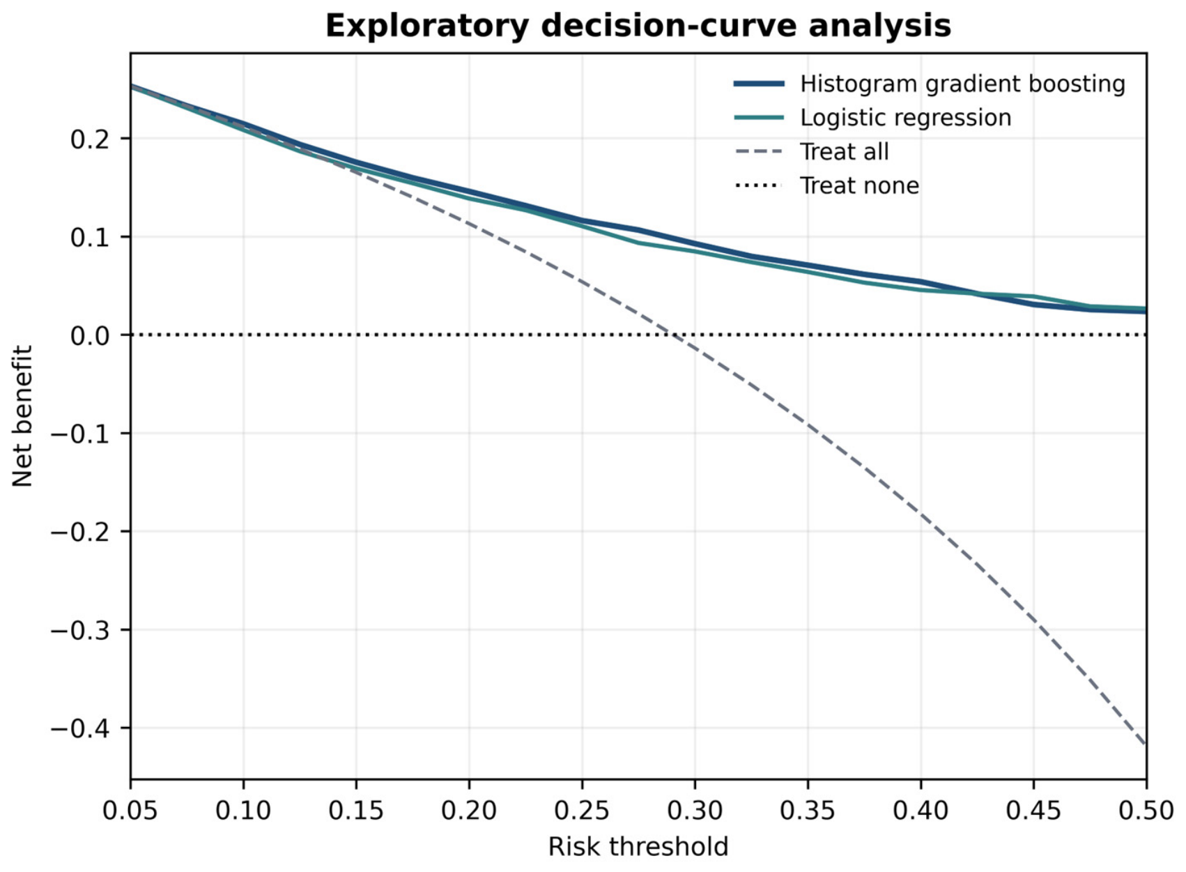
Decision-curve analysis was calculated across risk thresholds from 0.05 to 0.50, with one potential alert opportunity per patient. Decision curves summarize net benefit by weighting false positives according to the chosen threshold [29,30]. Because no clinical threshold-preference study or prospective intervention was performed, the decision-curve results were treated as exploratory rather than evidence of clinical benefit. External validation is needed to assess transportability beyond the development data [31].

2.9. Post Hoc Robustness and Ascertainment Audit

After the initial test evaluation, a second audit reused saved test risks and the original validation-selected threshold. No model was retrained or recalibrated and no threshold was changed. Frozen-model subsets examined complete 48 h ICU observation, symmetric final-laboratory requirements of 12 and 6 h applied to both positive and negative cases, exclusion of an observed pre-ICU qualifying creatinine rise, exclusion of post-landmark dialysis, exclusion of late qualifying results, age groups, recorded sex groups, albumin measurement status, and post-landmark creatinine measurement count. The complete 48 h observation subset also selected patients according to subsequent ICU stay duration. The symmetric 12 h and 6 h analyses applied the corresponding final-laboratory requirement to positive cases as well as negative cases and therefore changed the composition of the evaluated cohort rather than eliminating observation-dependent ascertainment.

The observed pre-ICU rise flag identified any qualifying creatinine rise whose qualifying measurement occurred before ICU admission, using creatinine chart time within the available index-hospitalization history. These patients remained eligible for the primary analysis because the primary prevalent-rise exclusion applied to qualifying rises observed from ICU admission through the 24 h landmark. Accordingly, a post-landmark qualifying creatinine rise in these patients could represent persistence or worsening of an earlier episode rather than a clinically confirmed incident AKI episode. For outcome timing, creatinine chart time determined whether a qualifying rise occurred within the post-landmark observation window. A late qualifying result was defined, among positive cases, when the first qualifying post-landmark creatinine measurement had no recorded storage time or when its earliest storage time occurred after the patient-specific observation endpoint. This flag was used only for post hoc sensitivity analysis and did not alter the original outcome labels.

Subgroup analyses were descriptive and were suppressed when fewer than 10 events or non-events were available. A separate comparison described the 15,231 included patients versus 15,900 patients who passed the renal and pre-landmark creatinine rules but had indeterminate outcomes. These patients were not assumed to be event-free, and the comparison was not interpreted as establishing model performance in the indeterminate group. Because true outcomes were not observed in the indeterminate group under the study ascertainment rules, we did not assign hypothetical outcome labels or estimate predictive performance in these patients.

Standardized mean differences (SMDs) were calculated for baseline and observation-process variables. For continuous variables, SMDs were calculated using observed values and pooled within-group standard deviations even when descriptive summaries were presented as medians and interquartile ranges; missingness was reported separately. Follow-up duration and post-landmark measurement counts were treated as ascertainment descriptors, not baseline predictors. EHR measurement and ordering processes can encode aspects of clinical workflow and illness state [32], so these comparisons were used to see mechanism visible rather than to claim that selection bias had been removed.

2.10. Transparency Scope

The transparency goal was model-level transparency rather than patient-level explanation or causal interpretation. The analysis therefore emphasized an interpretable logistic-regression comparator, a lean random forest, explicit calibration, fixed-threshold behavior, subgroup robustness, and audit of the outcome-observation process. The vancomycin ablation was performed only within the random-forest model family and therefore assessed the incremental contribution of that feature within the random forest; it does not establish the selected histogram gradient-boosting model’s dependence on vancomycin. We did not compute SHAP, LIME, counterfactual explanations, or clinician-rated explanations. Post hoc feature-attribution methods can describe aspects of model behavior, but such analyses were outside the scope of this study and should not be interpreted as mechanistic or clinically validated explanations [15,16,17].

2.11. Software

The execution environment used Google Colaboratory (Google Colab; google-colab package version 1.0.0) Python 3.13.15, pandas 2.2.3, NumPy 2.1.3, and scikit-learn 1.6.1. The fixed random seed was 20260908. The Supplementary Materials include executable code for the primary development and validation pipeline, executable code for the post hoc audit, and aggregate primary and audit outputs. These materials document data extraction, variable and unit mappings, outcome construction, cohort construction, data partitioning, preprocessing, complete model settings, calibration, threshold selection, and generation of the reported audit results and figures.

3. Results

3.1. Cohort Construction and Partitions

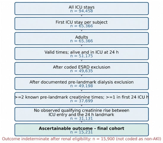
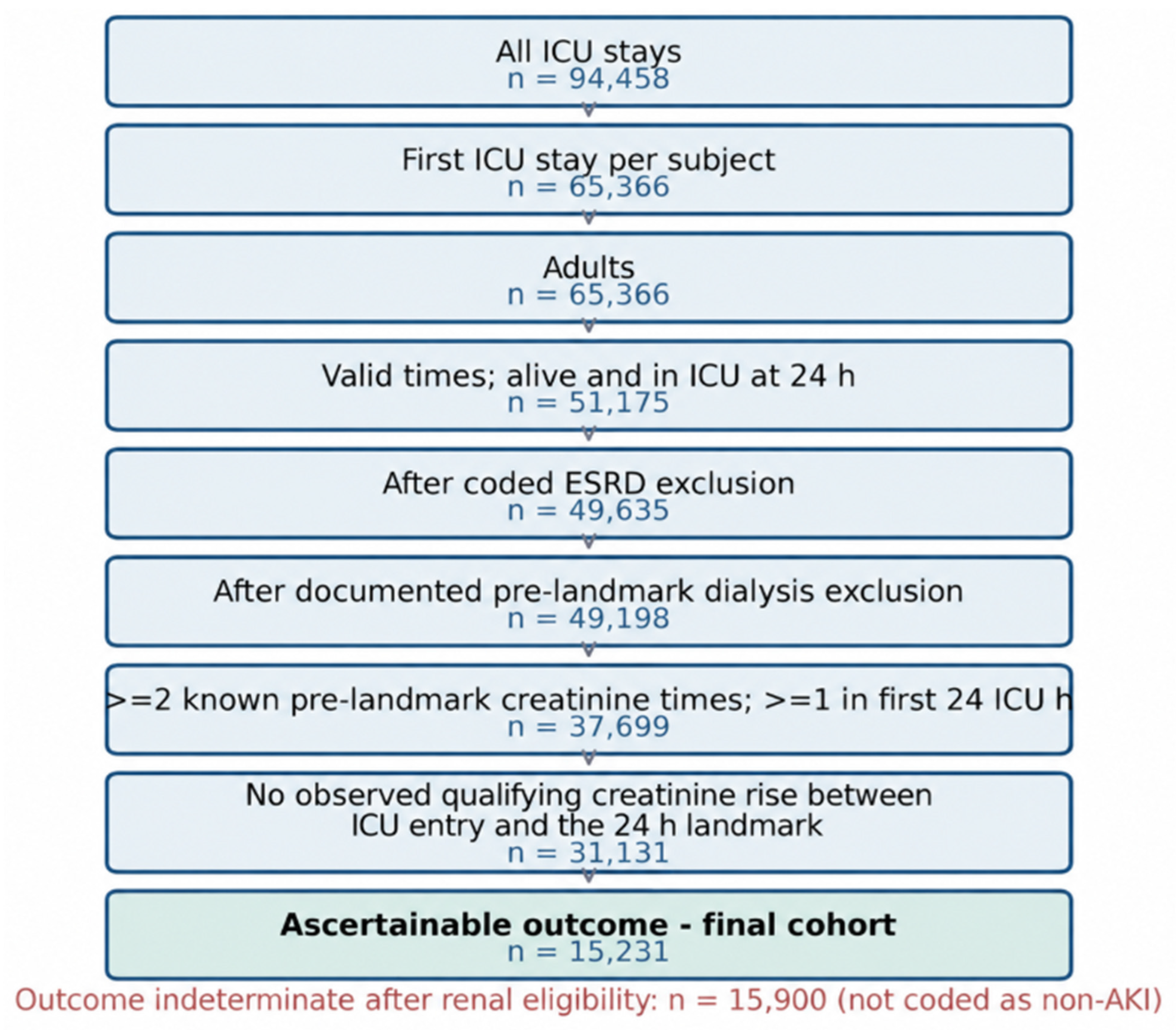
The source contained 94,458 ICU stays. Restricting to the first ICU stay per subject left 65,366 stays. After requiring valid times and survival/presence in the ICU at the 24 h landmark, 51,175 patients remained. Coded end-stage renal disease and documented pre-landmark dialysis exclusions left 49,198; pre-landmark creatinine eligibility left 37,699; and exclusion of an observed qualifying creatinine rise between ICU entry and the landmark left 31,131. Of these, 15,231 had an ascertainable post-landmark outcome and 15,900 were indeterminate (Figure 1). The final ascertainable cohort contained 4421 patients with a qualifying post-landmark creatinine rise (29.0%) and 10,810 observed-negative patients.

Figure 1. Cohort construction from all ICU stays to the final outcome-ascertainable cohort. The 15,900 indeterminate patients passed the pre-landmark renal eligibility rules but could not be assigned a positive or observed-negative outcome under the study observation rule.

Follow-up from the 24 h landmark to the patient-specific observation endpoint had a median of 48.0 h (IQR, 33.1–48.0) among patients with a qualifying rise and 48.0 h (IQR, 21.7–48.0) among observed-negative patients. The earliest observation endpoint involved ICU exit in 6184 patients (40.6%), hospital discharge in 688 (4.5%), and death in 244 (1.6%); 8357 patients (54.9%) reached the full 48 h horizon. Endpoint categories were not mutually exclusive when timestamps were identical: 241 patients had tied earliest endpoints, comprising 240 hospital-discharge/death ties and one ICU-exit/hospital-discharge/death tie. Among the 4421 patients with a qualifying post-landmark creatinine rise, the first qualifying measurement occurred a median of 12.6 h after the landmark (IQR, 5.3–21.1; 10th–90th percentile, 2.3–34.1 h).

Partition sizes were 9138 training patients with 2652 events, 2284 calibration patients with 663 events, 1523 validation patients with 442 events, and 2286 test patients with 664 events. Event prevalence was approximately 29% in every partition because the split was stratified. Selected predictor summaries were also similar across partitions (Table 1). Albumin was missing in roughly 70% of patients, whereas the routinely measured chemistry and blood-count variables had little missingness.

Table 1. Cohort partitions and selected predictor summaries.

Characteristic	Training	Calibration	Validation	Test
Patients	9138	2284	1523	2286
Qualifying creatinine-rise events	2652	663	442	664
Event prevalence	29.0%	29.0%	29.0%	29.0%
Age, years, median [IQR]	68.0 [56.0–78.0]	67.0 [56.0–78.0]	67.0 [56.0–77.0]	67.0 [56.0–77.0]
Creatinine, mg/dL, median [IQR]	0.9 [0.7–1.2]	0.9 [0.7–1.2]	0.9 [0.7–1.2]	0.9 [0.7–1.2]
BUN, mg/dL, median [IQR]	17.0 [12.0–27.0]	17.0 [12.0–27.0]	17.0 [12.0–28.0]	17.0 [12.0–27.0]
Glucose, mg/dL, median [IQR]	123.0 [104.0–149.0]	122.0 [103.0–149.0]	126.0 [107.0–152.0]	123.0 [104.0–149.0]
WBC, 109/L, median [IQR]	11.1 [8.3–14.7]	11.1 [8.1–14.7]	11.2 [8.2–14.8]	11.2 [8.3–14.8]
Albumin, g/dL, median [IQR]	3.2 [2.7–3.6]	3.2 [2.6–3.6]	3.1 [2.6–3.6]	3.1 [2.7–3.5]
Albumin missing	70.5%	69.7%	70.2%	69.5%

IQR, interquartile range; BUN, blood urea nitrogen; WBC, white blood cell count. Continuous summaries come from the frozen aggregate feature report; event prevalence is stratified by design.

3.2. Validation Selection and Held-Out Test Performance

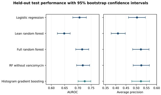
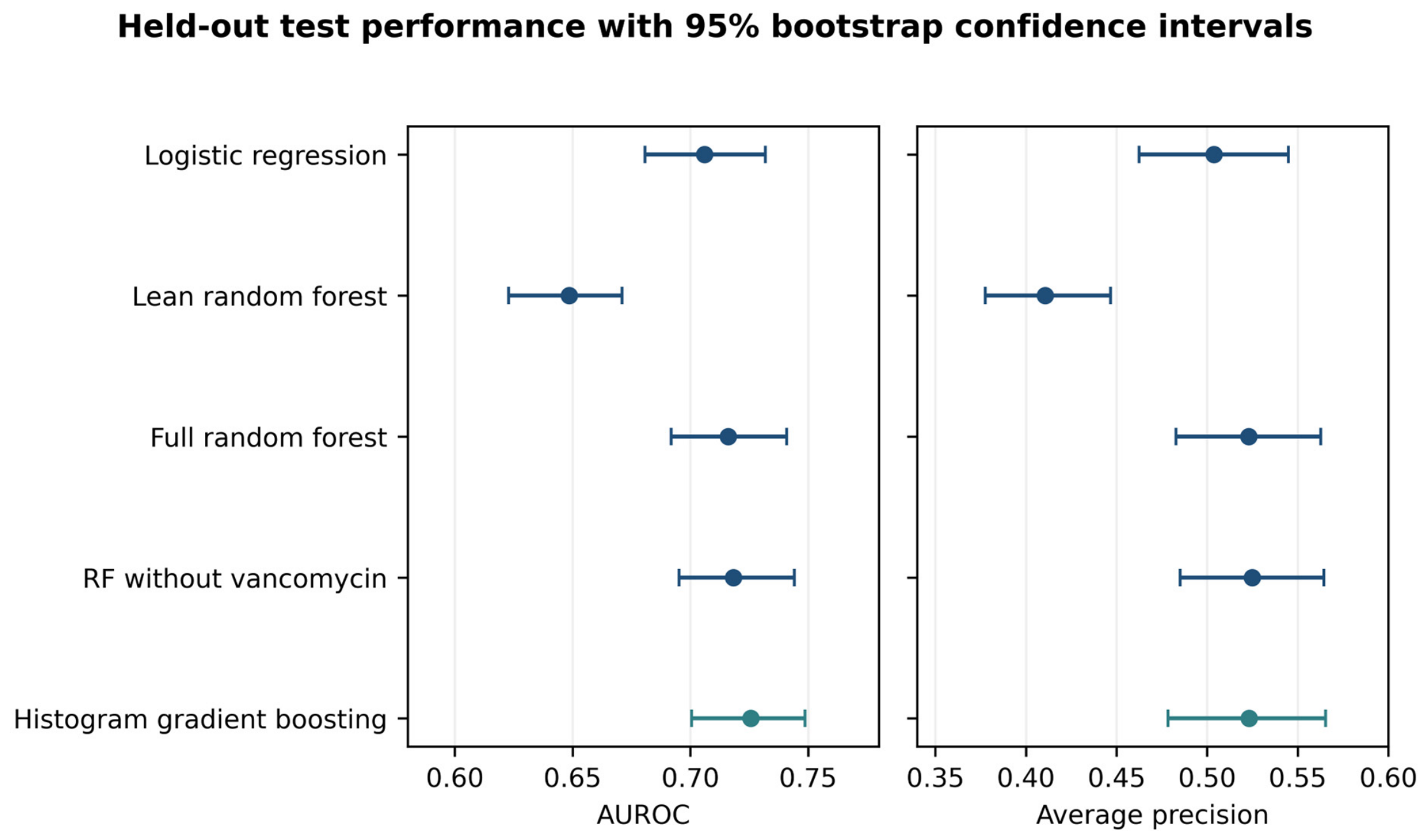
Histogram gradient boosting had the highest validation average precision (0.526) and was therefore selected before test scoring. In the held-out test set, using the primary 300-resample bootstrap analysis, histogram gradient boosting achieved AUROC 0.7257 (95% CI, 0.7005–0.7486), average precision 0.5232 (95% CI, 0.4784–0.5655), and Brier score 0.1785 (95% CI, 0.1708–0.1868) (Figure 2; Table 2). At the frozen threshold, sensitivity was 0.7846 (0.7507–0.8160), specificity 0.5222 (0.4997–0.5473), and PPV 0.4020 (0.3742–0.4280). The model generated 56.7 alerts per 100 patients, including 33.9 false alerts per 100 patients (95% CI, 31.7–35.8). The test confusion matrix was 847 true negatives, 775 false positives, 143 false negatives, and 521 true positives.

Figure 2. AUROC and average precision in the reserved test set. Error bars are 95% percentile bootstrap confidence intervals from 300 patient-level resamples with fitted models and thresholds held fixed. The prevalence-only reference is omitted from the figure for readability.

Table 2. Held-out test-set performance at validation-selected thresholds.

Model	AUROC	AP	Brier	Sens.	Spec.	PPV	False Alerts/100
Prevalence only	0.500	0.290	0.206	100.0%	0.0%	29.0%	71.0
Logistic regression	0.706	0.504	0.182	83.3%	42.4%	37.2%	40.9
Lean random forest	0.649	0.411	0.195	77.3%	44.5%	36.3%	39.4
Full random forest	0.716	0.523	0.180	79.7%	50.3%	39.6%	35.3
RF without vancomycin	0.718	0.525	0.179	78.0%	52.6%	40.2%	33.6
Histogram gradient boosting	0.726	0.523	0.179	78.5%	52.2%	40.2%	33.9

AP, average precision; Sens., sensitivity; Spec., specificity; PPV, positive predictive value. The histogram gradient-boosting threshold was 0.2164. Confidence intervals for the selected model are reported in the text and Figure 2. Threshold-specific metrics are not comparable to an unconstrained optimum because every threshold was fixed on validation data.

The full logistic model reached an AUROC of 0.7059 and an average precision of 0.5038. Using 2000 paired bootstrap resamples, the selected gradient-boosting model had an AUROC difference of +0.0197 versus logistic regression (95% CI, 0.00235 to 0.03571), an average-precision difference of +0.01948 (95% CI, −0.00551 to 0.04309), and a Brier-score difference of −0.00388 (95% CI, −0.00745 to 0.00002). Thus, the AUROC confidence interval excluded zero, whereas the average-precision and Brier-score confidence intervals included zero. Compared with the original 300-resample analysis, the interpretation of the AUROC and average-precision comparisons was unchanged, whereas the Brier-score confidence interval now included zero. At the validation-selected thresholds, histogram gradient boosting produced fewer false alerts than logistic regression (33.9 versus 40.9 per 100 patients) but also had lower test sensitivity (78.5% versus 83.3%), indicating a trade-off between false-alert burden and missed qualifying events. The random forest retrained without the vancomycin-order predictor performed similarly to the full random forest. The AUROC difference was +0.0023 (95% CI, −0.0017 to 0.0060), the average-precision difference was +0.0020 (−0.0045 to 0.0087), and the Brier difference was −0.00054 (−0.00142 to 0.00036). Within the random-forest model family, these results do not support a claim that predictive performance depended materially on that single order feature. This ablation does not establish the selected histogram gradient-boosting model’s dependence on vancomycin and does not estimate any causal medication effect.

3.3. Calibration and Exploratory Decision Curves

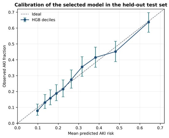
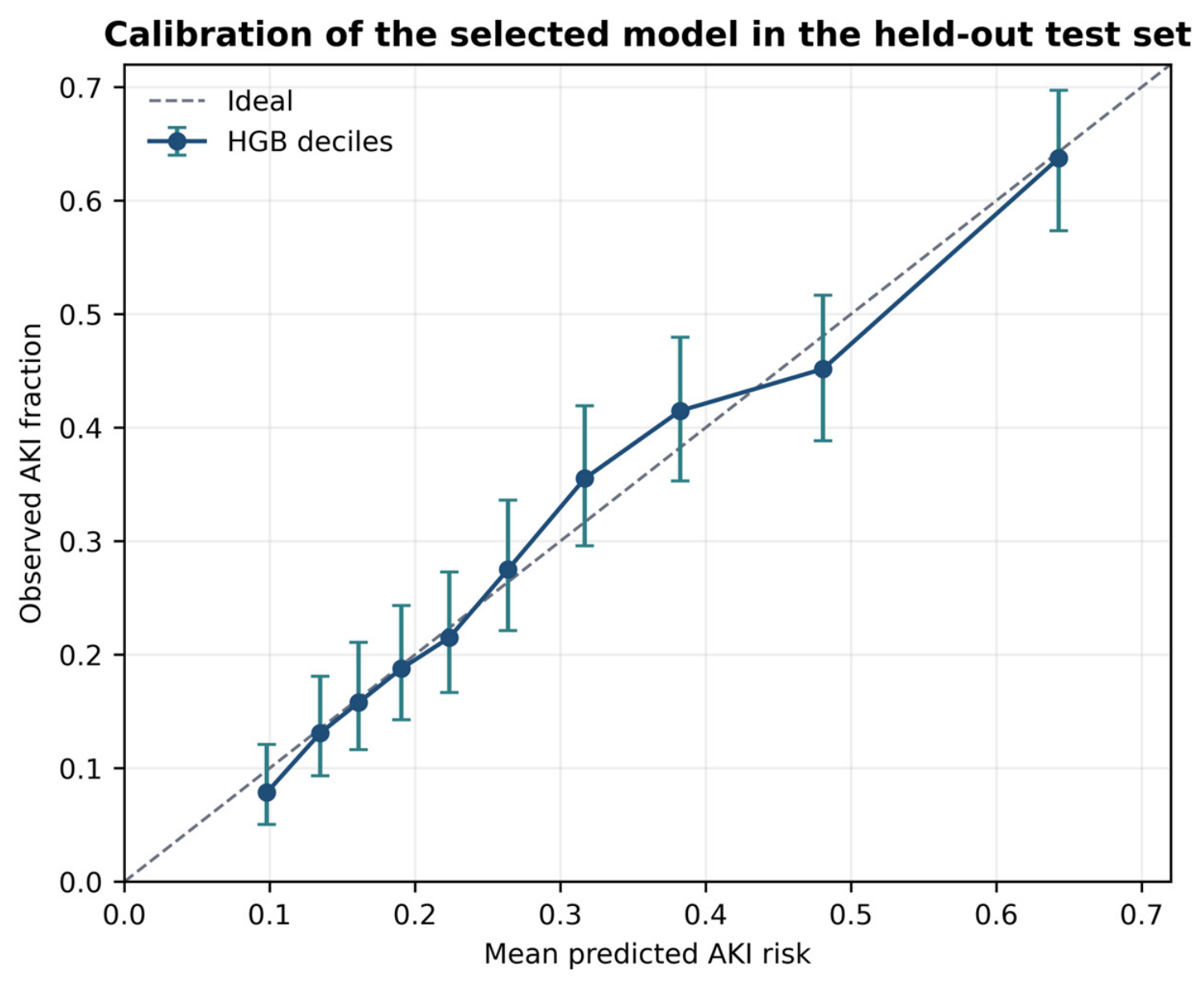
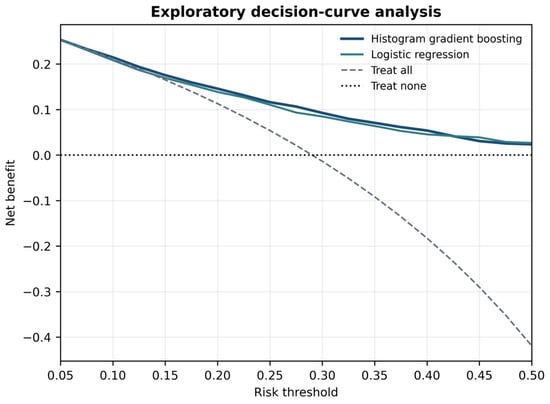
The selected model’s mean predicted probability in the test set was 0.2896, compared with an observed event fraction of 0.2905. The diagnostic calibration intercept was 0.023 (95% CI, −0.118 to 0.166), and the calibration slope was 1.022 (95% CI, 0.905 to 1.146). Decile-level observed event fractions generally tracked predicted risk, with some local departure in the middle-risk bins (Figure 3). These estimates describe internal test calibration and are not evidence that calibration will be preserved in another hospital or time period [27,31]. In exploratory decision-curve analysis, histogram gradient boosting had positive net benefit relative to treating none throughout the examined 0.05–0.50 threshold range and was above the treat-all strategy at the sampled thresholds (Figure 4). Full logistic regression was included in the decision-curve comparison. Because no clinically justified risk threshold was prespecified, individual thresholds were not selected post hoc to claim incremental clinical utility over logistic regression. This analysis does not establish clinical effectiveness because patient preferences, intervention harms, implementation costs, and the consequences of false alerts were not prospectively measured [29,30].

Figure 3. Decile calibration of the selected histogram gradient-boosting model in the held-out test set. Vertical bars are 95% Wilson confidence intervals for the observed event fraction. The dashed line is the ideal calibration.

Figure 4. Exploratory decision-curve analysis. Net benefit is shown for the selected model, full logistic regression, treat-all, and treat-none strategies across thresholds from 0.05 to 0.50. This analysis is not a prospective clinical-impact evaluation.

3.4. Frozen-Model Robustness Audit

The post hoc audit reproduced all 15,231 original patients and labels, and the selected model was not retrained, recalibrated, or retuned. Under complete 48 h observation, AUROC was 0.7068, Brier score 0.1827, mean predicted risk 0.294 versus an observed event frequency of 0.291, specificity 50.0%, and false alerts 35.5 per 100 patients. Calibration intercept was −0.074 (95% CI, −0.257 to 0.117) and slope was 0.930 (0.777–1.107).

Under the symmetric 12 h rule, 493 events and all 1622 non-events were retained, excluding 171 events and no non-events. AUROC was 0.7252 but mean predicted risk was 0.283 versus an observed event frequency of 0.233; PPV fell to 33.2%, and false alerts increased to 36.6 per 100 patients. Calibration intercept was −0.285 (95% CI, −0.427 to −0.143) and slope was 1.017 (0.892–1.149). Under the symmetric 6 h rule, 223 events and 788 non-events were retained, while 441 events and 834 non-events were excluded; AUROC was 0.6965, PPV 30.8%, and false alerts 37.4 per 100 patients. Mean predicted risk was 0.272 versus an observed event frequency of 0.221, with a calibration intercept of −0.419 (95% CI, −0.660 to −0.189) and a slope of 0.877 (0.685–1.068). Thus, similar AUROC under some observation rules did not imply stable calibration or threshold performance.

For age <65 versus ≥65 years, AUROC was 0.7291 versus 0.7040 and sensitivity was 66.8% versus 84.2%. Specificity was 63.9% versus 41.7%, and false alerts were 28.1 versus 38.3 per 100 patients. Mean predicted risk and observed event frequency were 0.237 versus 0.222 in the younger group and 0.330 versus 0.343 in the older group. Calibration slopes were 1.136 (95% CI, 0.912–1.377) and 0.926 (0.785–1.084), respectively. The prevalence difference affects PPV but does not by itself explain the sensitivity difference; these subgroup findings are descriptive and not causal or fairness conclusions.

AUROC was 0.7284 after excluding the observed pre-ICU rise flag, 0.7251 after excluding post-landmark dialysis, and 0.7262 after excluding late qualifying results. Recorded-sex, albumin-measurement, and creatinine-count subgroup analyses remained descriptive and post hoc, with no multiplicity adjustment (Figure 5).

Figure 5. Frozen-model discrimination robustness audit. Points show AUROC estimates and horizontal bars show 95% percentile bootstrap confidence intervals from the post hoc 1000-resample audit using frozen test-set predictions. The dashed vertical line indicates the original test-set AUROC. These analyses assess discrimination only; calibration and threshold-based performance are reported separately in Table 3 and the text.

Figure 5. Frozen-model discrimination robustness audit. Points show AUROC estimates and horizontal bars show 95% percentile bootstrap confidence intervals from the post hoc 1000-resample audit using frozen test-set predictions. The dashed vertical line indicates the original test-set AUROC. These analyses assess discrimination only; calibration and threshold-based performance are reported separately in Table 3 and the text.

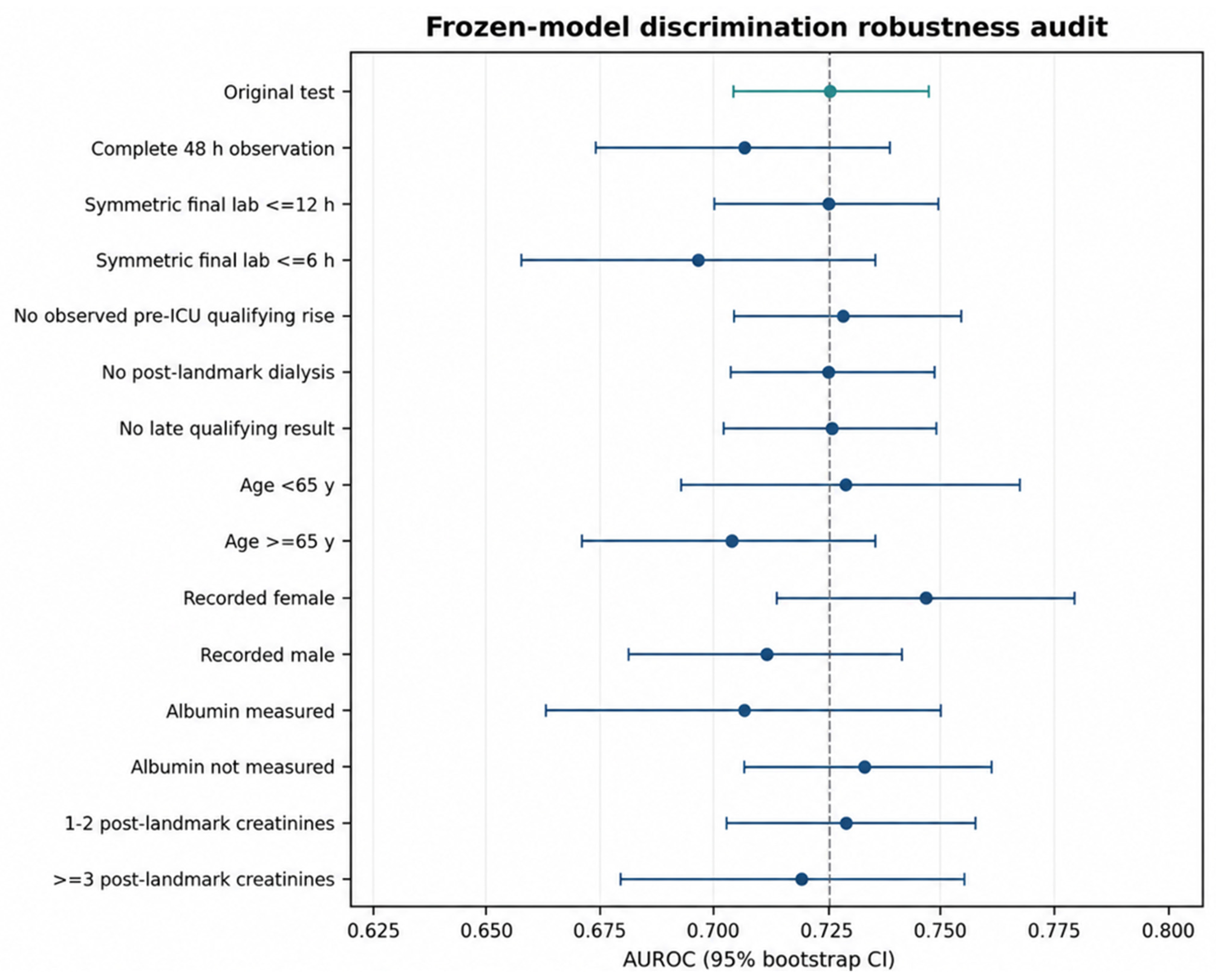
Table 3. Post hoc frozen-model sensitivity and subgroup analyses.

Subset	n	Event Frequency	AUROC (95% CI)	Sensitivity	Specificity	PPV	False Alerts/ 100	Mean Predicted Risk	Brier	Calibration Intercept (95% CI)	Calibration Slope (95% CI)
Original test	2286	29.0%	0.726 (0.704–0.747)	78.5%	52.2%	40.2%	33.9	0.290	0.1785	0.023 (−0.118 to 0.166)	1.022 (0.905–1.146)
Complete 48 h observation	1162	29.1%	0.707 (0.674–0.739)	77.5%	50.0%	38.9%	35.5	0.294	0.1827	−0.074 (−0.257 to 0.117)	0.930 (0.777–1.107)
Symmetric final lab <=12 h	2115	23.3%	0.725 (0.700–0.749)	78.3%	52.2%	33.2%	36.6	0.283	0.1589	−0.285 (−0.427 to −0.143)	1.017 (0.892–1.149)
Symmetric final lab <=6 h	1011	22.1%	0.697 (0.658–0.736)	75.3%	52.0%	30.8%	37.4	0.272	0.1608	−0.419 (−0.660 to −0.189)	0.877 (0.685–1.068)
No observed pre-ICU qualifying rise	2214	28.9%	0.728 (0.705–0.754)	78.1%	53.3%	40.5%	33.2	-	0.1776	-	-
No post-landmark dialysis	2277	28.9%	0.725 (0.704–0.749)	78.2%	52.3%	39.9%	33.9	-	0.1780	-	-
No late qualifying result	2276	28.7%	0.726 (0.702–0.749)	78.4%	52.2%	39.8%	34.1	-	0.1773	-	-
Age <65 y	990	22.2%	0.729 (0.693–0.767)	66.8%	63.9%	34.6%	28.1	0.237	0.1512	0.051 (−0.238 to 0.336)	1.136 (0.912–1.377)
Age >=65 y	1296	34.3%	0.704 (0.671–0.736)	84.2%	41.7%	42.9%	38.3	0.330	0.1994	0.016 (−0.148 to 0.184)	0.926 (0.785–1.084)
Recorded female	961	26.7%	0.747 (0.714–0.779)	79.0%	53.3%	38.2%	34.2	-	0.1665	-	-
Recorded male	1325	30.7%	0.712 (0.681–0.741)	78.1%	51.4%	41.6%	33.7	-	0.1872	-	-
Albumin measured	698	27.7%	0.707 (0.663–0.750)	76.2%	52.9%	38.2%	34.1	-	0.1784	-	-
Albumin not measured	1588	29.7%	0.733 (0.707–0.761)	79.4%	51.9%	41.1%	33.8	-	0.1785	-	-
1 – 2 post-landmark creatinines	1540	29.4%	0.729 (0.703–0.758)	77.9%	53.0%	40.8%	33.2	-	0.1783	-	-
>=3 post – landmark creatinines	746	28.4%	0.719 (0.680–0.755)	79.7%	50.6%	39.0%	35.4	-	0.1789	-	-

PPV varies with event prevalence and the distribution of predicted risks at the fixed threshold. Sensitivity is not determined by prevalence; differences in sensitivity across subgroups reflect differences in the distribution of model scores among patients with events when the same globally selected threshold is applied and may also reflect case-mix differences.

Table 3. Post hoc frozen-model sensitivity and subgroup analyses.

Subset	n	Event Frequency	AUROC (95% CI)	Sensitivity	Specificity	PPV	False Alerts/ 100	Mean Predicted Risk	Brier	Calibration Intercept (95% CI)	Calibration Slope (95% CI)
Original test	2286	29.0%	0.726 (0.704–0.747)	78.5%	52.2%	40.2%	33.9	0.290	0.1785	0.023 (−0.118 to 0.166)	1.022 (0.905–1.146)
Complete 48 h observation	1162	29.1%	0.707 (0.674–0.739)	77.5%	50.0%	38.9%	35.5	0.294	0.1827	−0.074 (−0.257 to 0.117)	0.930 (0.777–1.107)
Symmetric final lab <=12 h	2115	23.3%	0.725 (0.700–0.749)	78.3%	52.2%	33.2%	36.6	0.283	0.1589	−0.285 (−0.427 to −0.143)	1.017 (0.892–1.149)
Symmetric final lab <=6 h	1011	22.1%	0.697 (0.658–0.736)	75.3%	52.0%	30.8%	37.4	0.272	0.1608	−0.419 (−0.660 to −0.189)	0.877 (0.685–1.068)
No observed pre-ICU qualifying rise	2214	28.9%	0.728 (0.705–0.754)	78.1%	53.3%	40.5%	33.2	-	0.1776	-	-
No post-landmark dialysis	2277	28.9%	0.725 (0.704–0.749)	78.2%	52.3%	39.9%	33.9	-	0.1780	-	-
No late qualifying result	2276	28.7%	0.726 (0.702–0.749)	78.4%	52.2%	39.8%	34.1	-	0.1773	-	-
Age <65 y	990	22.2%	0.729 (0.693–0.767)	66.8%	63.9%	34.6%	28.1	0.237	0.1512	0.051 (−0.238 to 0.336)	1.136 (0.912–1.377)
Age >=65 y	1296	34.3%	0.704 (0.671–0.736)	84.2%	41.7%	42.9%	38.3	0.330	0.1994	0.016 (−0.148 to 0.184)	0.926 (0.785–1.084)
Recorded female	961	26.7%	0.747 (0.714–0.779)	79.0%	53.3%	38.2%	34.2	-	0.1665	-	-
Recorded male	1325	30.7%	0.712 (0.681–0.741)	78.1%	51.4%	41.6%	33.7	-	0.1872	-	-
Albumin measured	698	27.7%	0.707 (0.663–0.750)	76.2%	52.9%	38.2%	34.1	-	0.1784	-	-
Albumin not measured	1588	29.7%	0.733 (0.707–0.761)	79.4%	51.9%	41.1%	33.8	-	0.1785	-	-
1 – 2 post-landmark creatinines	1540	29.4%	0.729 (0.703–0.758)	77.9%	53.0%	40.8%	33.2	-	0.1783	-	-
>=3 post – landmark creatinines	746	28.4%	0.719 (0.680–0.755)	79.7%	50.6%	39.0%	35.4	-	0.1789	-	-

PPV varies with event prevalence and the distribution of predicted risks at the fixed threshold. Sensitivity is not determined by prevalence; differences in sensitivity across subgroups reflect differences in the distribution of model scores among patients with events when the same globally selected threshold is applied and may also reflect case-mix differences.

3.5. Outcome Indeterminacy and the Observation Process

The most important audit finding concerned outcome ascertainment. Among 31,131 patients remaining after the pre-landmark renal criteria, 15,900 had indeterminate outcomes. Of these, 7775 had no post-landmark creatinine measurement and 8125 had at least one post-landmark creatinine measurement, but the last measurement occurred too early to satisfy the negative observation rule.

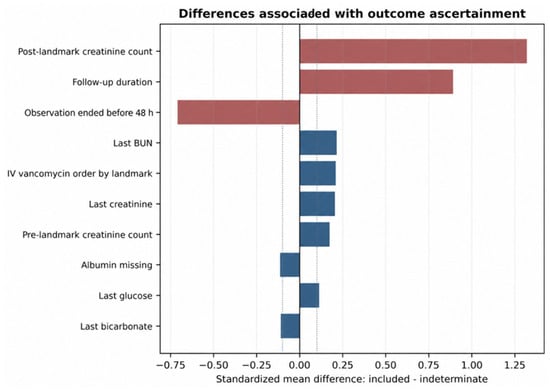
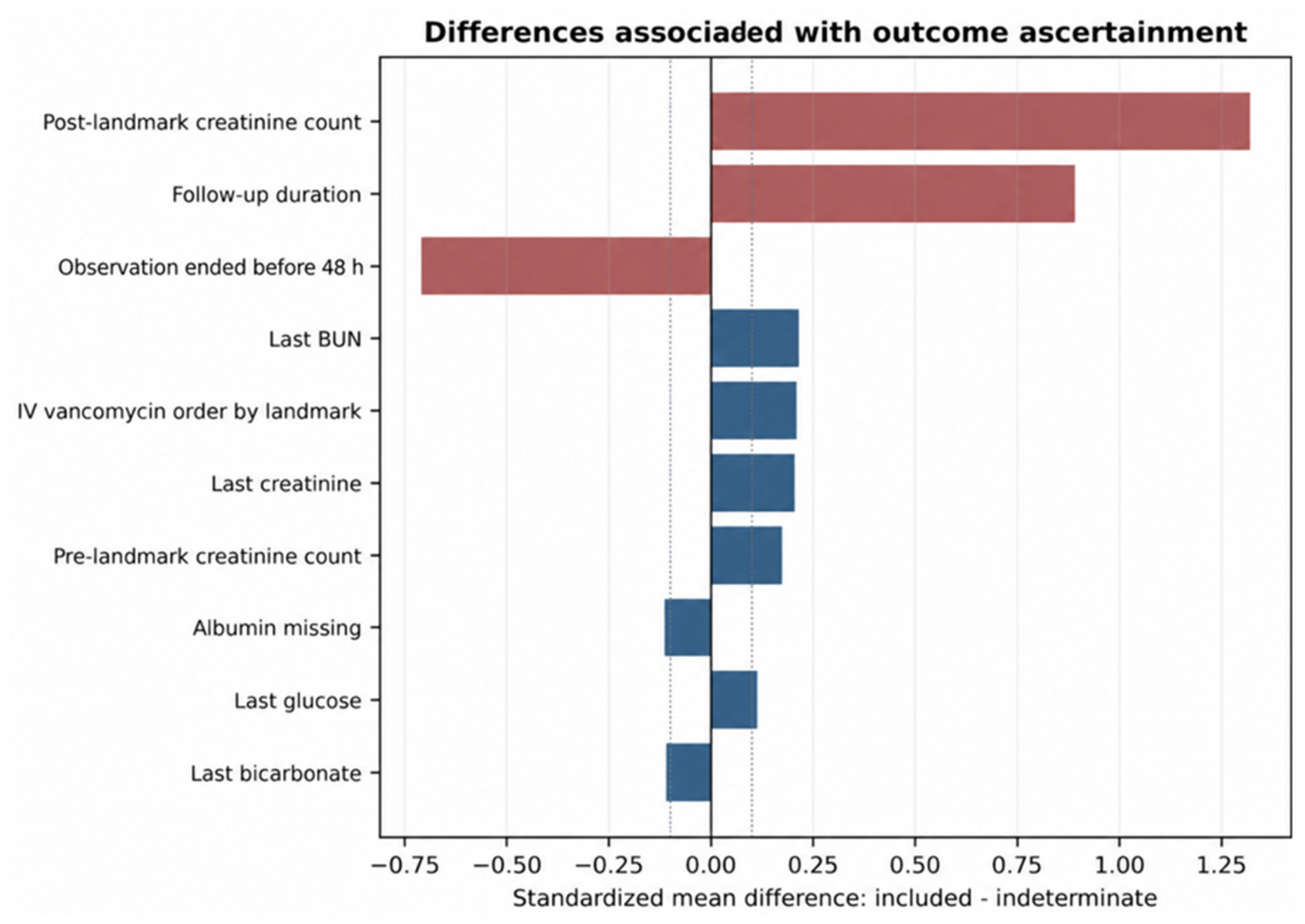
Included and indeterminate patients differed substantially in follow-up and measurement intensity (Table 4; Figure 6). Mean follow-up after the landmark was 37.0 h in included patients versus 22.4 h in indeterminate patients (SMD 0.891). Mean post-landmark creatinine measurement count was 2.81 versus 0.94 (SMD 1.319). Observation ended before 48 h in 45.1% of included patients versus 77.7% of patients with indeterminate outcomes (SMD −0.709). This measure includes observations terminated before 48 h because of ICU exit, hospital discharge, or death.

Table 4. Included versus outcome-indeterminate patients.

Variable	Included n = 15,231	Indeterminate n = 15,900	SMD
Age, years	67.0 [56.0–78.0]	66.0 [55.0–77.0]	0.075
IV vancomycin order by landmark	32.8%	23.4%	0.210
Pre-landmark creatinine count	3.0 [2.0–4.0]	2.0 [2.0–4.0]	0.171
Follow-up, h	48.0 [24.7–48.0]	18.6 [5.3–44.3]	0.891
Post-landmark creatinine count	2.0 [2.0–4.0]	1.0 [0.0–2.0]	1.319
Observation ended before 48 h	45.1%	77.7%	−0.709
Last creatinine, mg/dL	0.9 [0.7–1.2]	0.8 [0.7–1.1]	0.205
Last BUN, mg/dL	17.0 [12.0–27.0]	15.0 [11.0–22.0]	0.215
Albumin missing	70.2%	75.3%	−0.113

Continuous variables are median [IQR]; binary variables are percentages. SMD is included minus indeterminate. Follow-up and post-landmark measurement variables describe the outcome-observation process and were not baseline predictors.

Figure 6. Standardized mean differences between included patients and otherwise eligible patients with indeterminate outcomes. Large differences in follow-up and post-landmark creatinine measurement count indicate that outcome ascertainability was strongly related to the observation process.

Differences in age and recorded sex were small, but there were moderate differences in the vancomycin-order indicator, pre-landmark creatinine count, last creatinine, and last BUN. These findings show that the ability to assign an outcome was strongly related to subsequent observation and care processes. They cannot reveal the true AKI status of indeterminate patients or correct selection on their own.

4. Discussion

This study developed and internally validated several models for newly observed creatinine-defined AKI after a fixed 24 h ICU landmark and then subjected the selected model to a frozen-prediction audit. Four findings matter. First, histogram gradient boosting provided moderate discrimination, with a test AUROC of 0.726 and an average precision of 0.523. Second, aggregate calibration was close in the held-out test set, with mean predicted risk almost identical to event prevalence and a calibration slope near one. Third, the nonlinear model showed a modest improvement in AUROC, while the Brier-score difference was small and its confidence interval included zero. Fourth, and most importantly, outcome ascertainment depended strongly on post-landmark observation: more than 15,000 otherwise eligible patients could not be labeled under the study’s negative-outcome rule, and those patients had shorter follow-up and fewer creatinine measurements.

The discrimination estimate is within the broad range reported for EHR-based AKI prediction, but direct numerical comparisons across studies should be approached with caution. Earlier studies have used different settings, prediction times, horizons, baseline definitions, KDIGO implementations, and predictor sets [4,5,6,7,8]. Some reported higher AUROCs, including models using richer longitudinal or multisite data [4,8], but systematic reviews show that heterogeneity is large and that many AKI prediction studies have substantial risk of bias or limited external validation [9,10,11,12]. Our narrower feature set and strict timing rules were chosen to make availability at the landmark explicit rather than to maximize apparent performance.

The gradient-boosting model improved AUROC by about 0.02 and Brier score by about 0.004. In the fixed internal test sample, the 2000-resample paired-bootstrap confidence interval excluded zero for the AUROC difference, whereas the confidence intervals for the average-precision and Brier-score differences included zero. The incremental performance advantage should therefore be interpreted as modest and metric-dependent. In clinical prediction, a simpler model can remain attractive when performance is close because its form is easier to inspect, reproduce, and transport. This is consistent with broader arguments that high-stakes AI should not treat model complexity as a goal [15].

The transparency framing of this study therefore needs a precise boundary. This study did not generate patient-level SHAP, LIME, counterfactual, or causal explanations. Instead, it contributes transparency at the model-development and validation level: a simple comparator, a lean model, a true retraining-based vancomycin ablation, explicit probability calibration, a prespecified validation threshold, and robustness checks that expose the effects of observation choices. This distinction matters because post hoc feature-attribution plots can be useful descriptions of model behavior without proving clinical reasoning, causality, or safety [16,17]. Recent AKI XAI work demonstrates the value of feature-attribution methods for identifying model-associated biomarkers [13], while the 2026 GLASS-AKI review emphasizes that explanation methods still require stronger clinical validation and workflow integration [14]. A future extension of this work should add explanation stability and clinician evaluation using patient-level predictions, not simply attach an attribution method to the current aggregate analysis.

Calibration deserves similar emphasis. AUROC measures ranking, not whether a predicted 30% risk corresponds to an observed 30% event rate. Poor calibration can make a model misleading even when discrimination is acceptable [27]. The selected model showed reassuring internal calibration diagnostics, but these should not be generalized beyond the test sample. Random internal splits preserve much of the same clinical environment in development and test data, whereas temporal or external validation tests whether performance survives changes in patient mix, practice, measurement, and coding [31]. This paper should therefore be read as internal validation, not evidence of transportability.

The ascertainment audit is arguably the most important contribution. The negative label required a late-enough creatinine measurement, while a positive label could be detected earlier. This asymmetric rule protects against calling an unobserved patient a non-event, but it also creates an observation-dependent analytic cohort. The large SMDs for follow-up and post-landmark creatinine count show that included patients were much more intensively observed. EHR data are generated by care processes, and the presence and timing of measurements can themselves carry clinical information [32]. A model trained only among patients whose outcomes are observable may therefore learn a risk relationship that applies most directly to a monitored subgroup rather than to every ICU patient alive at 24 h.

The symmetric-observation and complete-horizon analyses help assess this concern but do not solve it. Requiring similar late-lab observation for both classes reduced the sample and, under the strict 6 h rule, lowered AUROC to about 0.70. The complete 48 h observation subset also had AUROC about 0.71. These results are not a failure of the model; they are evidence that the estimand changes when follow-up and measurement rules change. Future studies could define a prospectively enforceable observation schedule, use outcomes supported by multiple data sources, or consider methods that explicitly model informative observation and competing events.

The decision-curve analysis suggests that the selected model could offer net benefit under the mathematical assumptions used, but it should not be presented as proof that an alert would help patients. A randomized multicenter trial of EHR alerts for already-detected AKI found no improvement in the composite of AKI progression, dialysis, or death overall [33]. Prediction before AKI is a different intervention, but the lesson is relevant: model performance and alert effectiveness are separate questions. Prospective workflow studies would need to define who sees the prediction, what action is recommended, how repeated alerts are handled, and whether benefits outweigh false alerts and treatment burden.

This analysis has several strengths. Information leakage was reduced by requiring both laboratory chart time and storage time to be at or before the prediction landmark. Patients were separated across training, calibration, validation, and test partitions. Calibration and threshold selection were separated from model fitting. The model choice was made on validation data before test scoring. Confidence intervals used patient-level resampling, and paired comparisons preserved within-patient correlation. The later audit did not retrain the model or alter thresholds, so it probes the frozen model rather than optimizing retrospectively for a preferred result. The executed code, model specifications, and aggregate outputs also support reproducibility.

The limitations are substantial and should define the scope of the conclusions. First, MIMIC-IV is a single-center data source, and the random split provides internal validation only [21,31]. Second, the outcome captures only observed serum-creatinine changes and is not full KDIGO: urine output, dialysis-only AKI, outpatient historical baselines, and inferred normal baselines were not used [2]. Third, early ICU exit, hospital discharge, and death truncate follow-up, so the target is not an unconditional 48 h risk or a competing-risk model. Fourth, outcome indeterminacy was common and strongly associated with observation intensity. Fifth, end-stage kidney disease and dialysis exclusions rely on specific coding/procedure sources and may be incomplete. Sixth, the vancomycin feature reflects a prescription order, not administration or causal exposure. Seventh, age >=90 years is top-coded. Eighth, the predictor set emphasizes routinely measured laboratory summaries and does not exploit richer time series, physiology, diagnoses, or text. Ninth, subgroup and audit analyses were post hoc and unadjusted for multiplicity. Tenth, bootstrap intervals condition on the fixed developed model and do not capture the uncertainty of repeating the entire development process. Finally, no patient-level explanation validation, clinician study, prospective deployment, or clinical-impact trial was performed.

The next step should not be another round of optimization on this test set. A stronger study would freeze the current model and protocol, evaluate it in a calendar-separated MIMIC cohort if a valid temporal design can be constructed, then test it in an external ICU database with harmonized outcome ascertainment. In parallel, patient-level explanation methods could be added and evaluated for stability across sites and for whether clinicians correctly understand the explanations. Such work would move the model from transparent internal development toward genuinely explainable and trustworthy clinical AI.

5. Conclusions

A histogram gradient-boosting model using first-24 h ICU data predicted a newly observed creatinine-defined qualifying rise after the landmark and before the earlier of 48 h or observation termination, with moderate discrimination and close aggregate calibration in an internal held-out test set. Its gain over logistic regression was modest.Frozen-model analyses showed broadly similar discrimination across several observation and subgroup checks (Figure 5), but calibration and threshold-based operating characteristics changed under some observation restrictions. The dominant limitation was outcome ascertainment: almost as many otherwise eligible patients had indeterminate outcomes as entered the final cohort, and ascertainability was strongly related to follow-up and creatinine measurement intensity. The results support transparent model development and robustness auditing, but not external validity, causal interpretation, validated patient-level explanations, or clinical effectiveness. External and temporal validation with prospectively defined observation rules should precede any clinical deployment.

References

- Kellum, J.A.; Romagnani, P.; Ashuntantang, G.; Ronco, C.; Zarbock, A.; Anders, H.-J. Acute kidney injury. Nat. Rev. Dis. Primers 2021, 7, 52. [Google Scholar] [CrossRef] [Scilit]
- Kidney Disease: Improving Global Outcomes (KDIGO) Acute Kidney Injury Work Group. KDIGO Clinical Practice Guideline for Acute Kidney Injury. Kidney Int. Suppl. 2012, 2, 1–138. [Google Scholar]
- Hoste, E.A.J.; Bagshaw, S.M.; Bellomo, R.; Cely, C.M.; Colman, R.; Cruz, D.N.; Edipidis, K.; Forni, L.G.; Gomersall, C.D.; Govil, D.; et al. Epidemiology of acute kidney injury in critically ill patients: The multinational AKI-EPI study. Intensive Care Med. 2015, 41, 1411–1423. [Google Scholar] [CrossRef] [Scilit]
- Fléchet, M.; Güiza, F.; Schetz, M.; Wouters, P.; Vanhorebeek, I.; Derese, I.; Gunst, J.; Spriet, I.; Casaer, M.; Berghe, G.V.D.; et al. AKIpredictor, an online prognostic calculator for acute kidney injury in adult critically ill patients: Development, validation and comparison to serum neutrophil gelatinase-associated lipocalin. Intensive Care Med. 2017, 43, 764–773. [Google Scholar] [CrossRef] [Scilit]
- Koyner, J.L.; Carey, K.A.; Edelson, D.P.; Churpek, M.M. The development of a machine learning inpatient acute kidney injury prediction model. Crit. Care Med. 2018, 46, 1070–1077. [Google Scholar] [CrossRef] [Scilit]
- Mohamadlou, H.; Lynn-Palevsky, A.; Barton, C.; Chettipally, U.; Shieh, L.; Calvert, J.; Saber, N.R.; Das, R. Prediction of acute kidney injury with a machine learning algorithm using electronic health record data. Can. J. Kidney Health Dis. 2018, 5, 2054358118776326. [Google Scholar] [CrossRef] [Scilit]
- Simonov, M.; Ugwuowo, U.; Moreira, E.; Yamamoto, Y.; Biswas, A.; Martin, M.; Testani, J.; Wilson, F.P. A simple real-time model for predicting acute kidney injury in hospitalized patients in the US: A descriptive modeling study. PLoS Med. 2019, 16, e1002861. [Google Scholar] [CrossRef] [Scilit]
- Tomašev, N.; Glorot, X.; Rae, J.W.; Zielinski, M.; Askham, H.; Saraiva, A.; Mottram, A.; Meyer, C.; Ravuri, S.; Protsyuk, I.; et al. A clinically applicable approach to continuous prediction of future acute kidney injury. Nature 2019, 572, 116–119. [Google Scholar] [CrossRef] [Scilit]
- Vagliano, I.; Chesnaye, N.C.; Leopold, J.H.; Jager, K.J.J.; Abu-Hanna, A.; Schut, M.C. Machine learning models for predicting acute kidney injury: A systematic review and critical appraisal. Clin. Kidney J. 2022, 15, 2266–2280. [Google Scholar] [CrossRef] [Scilit]
- Feng, Y.; Wang, A.Y.; Jun, M.; Pu, L.; Weisbord, S.D.; Bellomo, R.; Hong, D.; Gallagher, M. Characterization of risk prediction models for acute kidney injury: A systematic review and meta-analysis. JAMA Netw. Open 2023, 6, e2313359. [Google Scholar] [CrossRef] [Scilit]
- Shi, T.; Lin, Y.; Zhao, H.; Kong, G. Artificial intelligence models for predicting acute kidney injury in the intensive care unit: A systematic review of modeling methods, data utilization, and clinical applicability. JAMIA Open 2025, 8, ooaf065. [Google Scholar] [CrossRef] [Scilit]
- Wainstein, M.; Flanagan, E.; Johnson, D.W.; Shrapnel, S. Systematic review of externally validated machine learning models for predicting acute kidney injury in general hospital patients. Front. Nephrol. 2023, 3, 1220214. [Google Scholar] [CrossRef] [Scilit]
- Koozi, H.; Engström, J.; Friberg, H.; Frigyesi, A. Explainable AI identifies key biomarkers for acute kidney injury prediction in the ICU. Intensive Care Med. Exp. 2025, 13, 106. [Google Scholar] [CrossRef] [Scilit]
- Lin, W.-L.; Fang, S.-S.; Chen, S.-H. From black box to glass box: Explainable artificial intelligence for acute kidney injury prediction-a scoping review and the GLASS-AKI translational framework proposal. Int. Urol. Nephrol. 2026. online ahead of print. [Google Scholar] [CrossRef] [Scilit]
- Rudin, C. Stop explaining black box machine learning models for high stakes decisions and use interpretable models instead. Nat. Mach. Intell. 2019, 1, 206–215. [Google Scholar] [CrossRef] [Scilit]
- Ghassemi, M.; Oakden-Rayner, L.; Beam, A.L. The false hope of current approaches to explainable artificial intelligence in health care. Lancet Digit. Health 2021, 3, e745–e750. [Google Scholar] [CrossRef] [Scilit]
- Amann, J.; Blasimme, A.; Vayena, E.; Frey, D.; Madai, V.I.; Precise4Q Consortium. Explainability for artificial intelligence in healthcare: A multidisciplinary perspective. BMC Med. Inform. Decis. Mak. 2020, 20, 310. [Google Scholar] [CrossRef] [Scilit]
- Collins, G.S.; Moons, K.G.M.; Dhiman, P.; Riley, R.D.; Beam, A.L.; Van Calster, B.; Ghassemi, M.; Liu, X.; Reitsma, J.B.; van Smeden, M.; et al. TRIPOD+AI statement: Updated guidance for reporting clinical prediction models that use regression or machine learning methods. BMJ 2024, 385, e078378. [Google Scholar] [CrossRef] [Scilit]
- Moons, K.G.M.; Damen, J.A.A.; Kaul, T.; Hooft, L.; Navarro, C.A.; Dhiman, P.; Beam, A.L.; Van Calster, B.; Celi, L.A.; Denaxas, S.; et al. PROBAST+AI: An updated quality, risk of bias, and applicability assessment tool for prediction models using regression or artificial intelligence methods. BMJ 2025, 388, e082505. [Google Scholar] [CrossRef] [Scilit]
- Norgeot, B.; Quer, G.; Beaulieu-Jones, B.K.; Torkamani, A.; Dias, R.; Gianfrancesco, M.; Arnaout, R.; Kohane, I.S.; Saria, S.; Topol, E.; et al. Minimum information about clinical artificial intelligence modeling: The MI-CLAIM checklist. Nat. Med. 2020, 26, 1320–1324. [Google Scholar] [CrossRef] [Scilit]
- Johnson, A.E.W.; Bulgarelli, L.; Shen, L.; Gayles, A.; Shammout, A.; Horng, S.; Pollard, T.J.; Hao, S.; Moody, B.; Gow, B.; et al. MIMIC-IV, a freely accessible electronic health record dataset. Sci. Data 2023, 10, 1. [Google Scholar] [CrossRef] [Scilit]
- Johnson, A.; Bulgarelli, L.; Pollard, T.; Gow, B.; Moody, B.; Horng, S.; Celi, L.A.; Mark, R. MIMIC-IV (version 3.1). PhysioNet 2024. [Google Scholar] [CrossRef]
- Breiman, L. Random forests. Mach. Learn. 2001, 45, 5–32. [Google Scholar] [CrossRef] [Scilit]
- Friedman, J.H. Greedy function approximation: A gradient boosting machine. Ann. Stat. 2001, 29, 1189–1232. [Google Scholar] [CrossRef] [Scilit]
- Pedregosa, F.; Varoquaux, G.; Gramfort, A.; Michel, V.; Thirion, B.; Grisel, O.; Blondel, M.; Prettenhofer, P.; Weiss, R.; Dubourg, V. Scikit-learn: Machine learning in Python. J. Mach. Learn. Res. 2011, 12, 2825–2830. [Google Scholar]
- Platt, J.C. Probabilistic outputs for support vector machines and comparisons to regularized likelihood methods. In Advances in Large Margin Classifiers; Smola, A.J., Bartlett, P.L., Scholkopf, B., Schuurmans, D., Eds.; MIT Press: Cambridge, MA, USA, 1999; pp. 61–74. [Google Scholar]
- Van Calster, B.; McLernon, D.J.; van Smeden, M.; Wynants, L.; Steyerberg, E.W. Calibration: The Achilles heel of predictive analytics. BMC Med. 2019, 17, 230. [Google Scholar] [CrossRef] [Scilit]
- Saito, T.; Rehmsmeier, M. The precision-recall plot is more informative than the ROC plot when evaluating binary classifiers on imbalanced datasets. PLoS ONE 2015, 10, e0118432. [Google Scholar] [CrossRef] [Scilit]
- Vickers, A.J.; Elkin, E.B. Decision curve analysis: A novel method for evaluating prediction models. Med. Decis. Mak. 2006, 26, 565–574. [Google Scholar] [CrossRef] [Scilit]
- Vickers, A.J.; van Calster, B.; Steyerberg, E.W. A simple, step-by-step guide to interpreting decision curve analysis. Diagn. Progn. Res. 2019, 3, 18. [Google Scholar] [CrossRef] [Scilit]
- Steyerberg, E.W.; Harrell, F.E., Jr. Prediction models need appropriate internal, internal-external, and external validation. J. Clin. Epidemiol. 2016, 69, 245–247. [Google Scholar] [CrossRef] [Scilit]
- Agniel, D.; Kohane, I.S.; Weber, G.M. Biases in electronic health record data due to processes within the healthcare system: Retrospective observational study. BMJ 2018, 361, k1479. [Google Scholar] [CrossRef] [Scilit]
- Wilson, F.P.; Martin, M.; Yamamoto, Y.; Partridge, C.; Moreira, E.; Arora, T.; Biswas, A.; Feldman, H.; Garg, A.X.; Greenberg, J.H.; et al. Electronic health record alerts for acute kidney injury: Multicenter, randomized clinical trial. BMJ 2021, 372, m4786. [Google Scholar] [CrossRef] [Scilit]
Disclaimer/Publisher’s Note: The statements, opinions and data contained in all publications are solely those of the individual author(s) and contributor(s) and not of MDPI and/or the editor(s). MDPI and/or the editor(s) disclaim responsibility for any injury to people or property resulting from any ideas, methods, instructions or products referred to in the content. |
© 2026 by the authors. Licensee MDPI, Basel, Switzerland. This article is an open access article distributed under the terms and conditions of the Creative Commons Attribution (CC BY) license.