Ship Trajectory Clustering Method Considering Navigation Behavior Sequences

Abstract

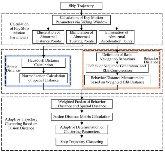
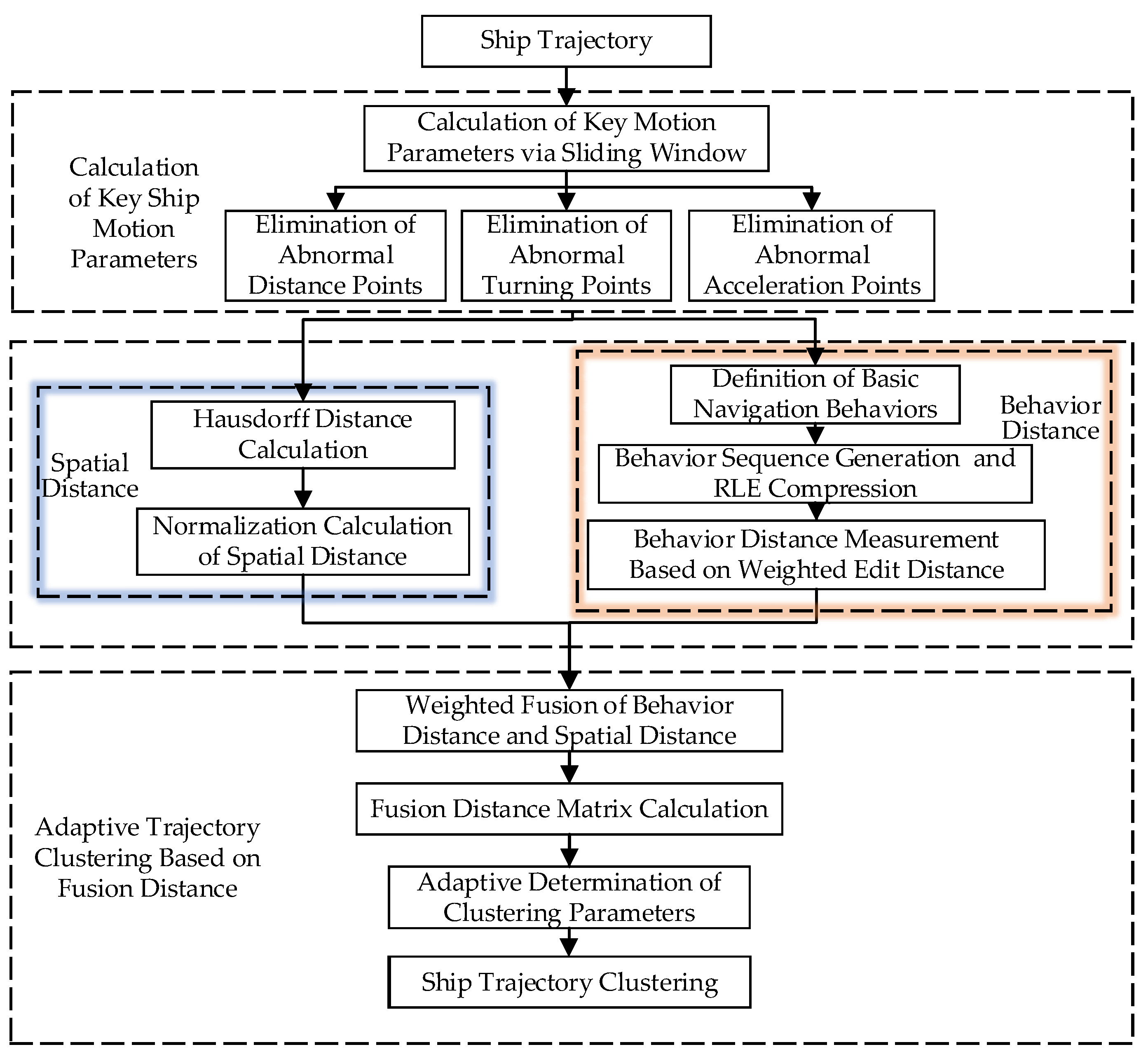
Existing ship trajectory clustering methods often overlook the impact of navigation behaviors (e.g., heading and speed variations) on clustering performance. To address this limitation, a novel ship trajectory clustering method that explicitly incorporates navigation behavior sequence is proposed. Firstly, ship trajectories are preprocessed, and key motion parameters, including the ship Rate Of Turn (ROT) and acceleration at each trajectory point, are calculated through a sliding window. Secondly, by integrating various motion parameters, the navigation behaviors corresponding to trajectory points are classified, and the classification results are taken as the core element to measure the behavior distance between different trajectories. Then, the spatial distance between trajectories is measured based on the Hausdorff distance. Finally, an adaptive Density-Based Spatial Clustering of Applications with Noise (DBSCAN) algorithm is adopted, which fuses behavior distance and spatial distance, to realize ship trajectory clustering that takes navigation behavior into account. Experimental results on Dalian Port and Yantai Port datasets show that: (1) Compared with the classical DBSCAN and Multi-dimensional Density-Based Trajectory Clustering of Applications with Noise (MD-DBTCAN) methods, the proposed method achieves finer granularity of clustering results; (2) Compared with the classical DBSCAN method, the proposed method can effectively distinguish straight-line navigation trajectories from trajectories with frequent turning behaviors; compared with the MD-DBTCAN method, the proposed method can distinguish normal straight-line navigation trajectories from trajectories with frequent acceleration and deceleration behaviors.

1. Introduction

The Automatic Identification System (AIS) continuously acquires dynamic and static information from ships via shore-based stations and satellite systems, generating massive ship trajectory data [1]. It provides data support for marine big data mining research, including ship behavior analysis, traffic flow prediction, and maritime supervision optimization [2]. As one of the key technical means for marine big data mining [3], ship trajectory clustering technology can effectively extract key navigation channels of ships by clustering massive ship trajectories and provide technical support for the mining of ship navigation rules and the optimization of maritime management [4].

At present, numerous scholars have carried out research on ship trajectory clustering and proposed a series of trajectory clustering algorithms [5,6,7]. Among them, the Density-Based Spatial Clustering of Applications with Noise (DBSCAN) algorithm is widely used because it does not require a preset number of clusters and can discover trajectory clusters of arbitrary shapes [8,9,10]. Zhang et al. [11] improved the DBSCAN method with a segmentation strategy, which divides long trajectories into feature sub-paths and performs density clustering based on them, solving the problems of local feature loss and low efficiency when the traditional DBSCAN method processes long trajectories. Wang et al. [12] improved the DBSCAN method combined with a hierarchical idea and realized multi-scale hierarchical extraction of trajectories by constructing a hierarchical density tree of trajectories. However, Shen et al. [13] noted that traditional Hausdorff distance cannot distinguish trajectories with identical spatial shapes but opposite directions. To solve this, they proposed a Cosine–Hausdorff distance by fusing course vector cosine similarity with spatial Hausdorff distance.

To further improve the representation capability for trajectory features, scholars have begun to explore trajectory representation learning methods based on deep learning and graph structure in recent years. Lian et al. [14] fused a deep autoencoder and a clustering network to iteratively complete ship trajectory clustering in a low-dimensional latent space. Murray et al. [15] used a Variational Recurrent Neural Network (VRNN) to generate implicit representations by learning the temporal position features of trajectories and extract main navigation routes. Mohamed et al. [16] combined a Graph Neural Network (GNN) to model sea area grids and trajectory heterogeneous graphs and realized ship navigation path clustering by learning the spatial adjacency relationships of trajectories. Zhang et al. [17] constructed a trajectory similarity graph combined with a Graph Attention Network (GAT) and used the attention mechanism to capture the local spatial dependencies between trajectories, which improved the clustering accuracy in dense water areas.

Trajectory clustering is not only a fundamental task for navigation pattern mining but also provides critical support for downstream maritime applications. Zhang et al. [11] combined trajectory clustering with abnormal navigation behavior detection, showing that accurate clustering can effectively identify deviant vessels in busy port waters. Baghizadeh et al. [18] applied AIS trajectory analysis to optimize vessel operations for offshore wind farm maintenance, demonstrating the practical engineering value of trajectory mining technology.

Although these methods have improved feature extraction capability, two key limitations remain. First, the model has low interpretability, and the implicit vector representation cannot correspond to the specific semantics of navigation behaviors. Second, ship maneuvering features such as heading and speed are not incorporated into the model as explicit structured parameters, making it unable to distinguish different navigation patterns.

To further consider the motion differences between ships, Xu et al. [19] introduced two instantaneous parameters, heading and speed, at the trajectory point level for clustering under the density framework. Liu et al. [20] realized clustering by extracting statistical values such as the mean and median of the heading and speed of the entire trajectory. An et al. [21] further proposed a Multi-dimensional Density-Based Trajectory Clustering of Applications with Noise (MD-DBTCAN) algorithm based on fusion distance measurement, which compresses trajectories to retain feature change points of heading and speed and then calculates the fusion distance respectively for clustering.

However, the above methods only consider two motion parameters, heading and speed, in trajectory clustering and have not fully exploited the potential of motion features. Li et al. [3] proposed an unsupervised maritime traffic pattern extraction method based on adaptive trajectory segmentation, which demonstrated that segment-level trajectory representation can better capture continuous motion patterns than point-level features. Reference [22] further analyzed the influence of ship rate of turn and acceleration on navigation and classified basic ship navigation behaviors. This provides a theoretical inspiration for making full use of ship rate of turn, acceleration and other factors to carry out trajectory clustering considering navigation behavior.

To address these research gaps, this paper proposes a ship trajectory clustering method considering navigation behavior sequence. The contributions are listed as follows:

(1)

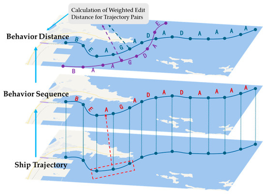
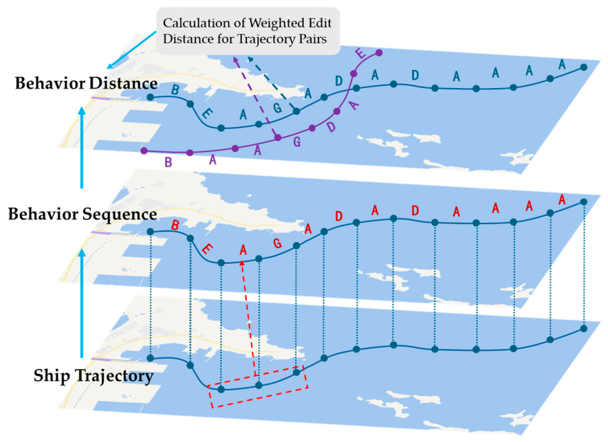
A novel behavior sequence representation method is proposed for ship trajectories, converting geometric trajectories into semantic behavior sequences based on seven basic navigation behaviors.

(2)

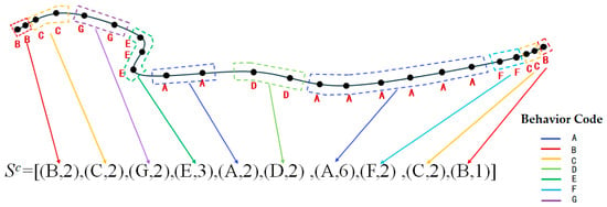
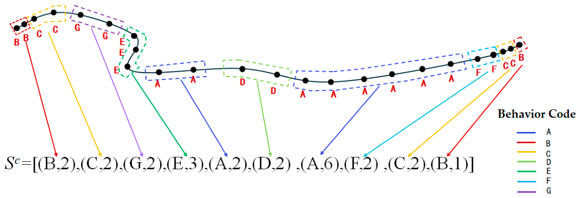
A weighted edit distance metric combined with Run-Length Encoding (RLE) compression is designed to measure similarity between behavior sequences, capturing temporal behavioral patterns while reducing computational complexity.

(3)

Behavioral distance and spatial distance are combined and incorporated into an adaptive DBSCAN clustering method, which automatically determines clustering parameters based on data distribution characteristics.

(4)

Experiments are conducted on two port datasets, demonstrating the effectiveness, generalization ability, and preliminary cross-port robustness of the proposed method.

2. Ship Trajectory Clustering Method Considering Navigation Behavior

The proposed method consists of three main stages: (1) calculation of key ship motion parameters, (2) measurement of behavior and spatial distances, and (3) adaptive trajectory clustering based on behavior–spatial fusion distance. The flowchart is shown in Figure 1.

Figure 1. Flowchart of the ship trajectory clustering method considering navigation behavior.

(1)

In the stage of calculating key ship motion parameters: first, the missing key motion parameters (turning angle, ship rate of turn, ship acceleration) in AIS data are calculated through a sliding window; then, three types of abnormal points are eliminated according to ship dynamic constraints, and drift points are eliminated by intersection with land data; finally, trajectories with the same Maritime Mobile Service Identity (MMSI) are split according to time intervals to obtain preprocessed ship trajectory data.

(2)

In the stage of measuring behavior distance and spatial distance: on the one hand, seven basic navigation behaviors are defined, the ship trajectory is converted into a behavior sequence based on three-level decision-making, the sequence is compressed by run-length encoding, and the behavior distance between trajectory pairs is calculated based on weighted edit distance; on the other hand, the spatial distance between trajectory pairs is calculated based on the Hausdorff distance.

(3)

In the stage of adaptive trajectory clustering based on behavior–spatial fusion distance: first, the behavior distance and spatial distance are weighted and fused to obtain the fusion distance, and the feature matrix is calculated; then, taking this matrix as input, the clustering parameter combination is adaptively determined based on its data distribution characteristics, and trajectory clustering is performed.

2.1. Calculation of Key Ship Motion Parameters

2.1.1. Calculation of Key Motion Parameters

The original AIS data covers basic navigation information, such as longitude, latitude, sailing speed and heading, but motion parameters characterizing the ship’s motion state, such as acceleration, turning angle and rate of turn, cannot be directly obtained and need to be calculated [23]. Since AIS data are essentially discrete time series, deriving motion parameters from only two adjacent points makes the results highly sensitive to noise from single-point fluctuations, which makes it difficult to truly reflect the continuous motion state of the ship. For this reason, a sliding window based on a fixed number of points is used to calculate ship motion parameters. Through local analysis of the continuous trajectory sequence, the long trajectory data is divided into a series of overlapping short window segments, and then, the calculation of each motion parameter is completed independently in each window. The symbol definition of the motion parameter calculation model is shown in Table 1.

Table 1. Symbol definition for the motion parameter calculation model.

Symbol	Definition	Unit
w	Window size	-
θ	Ship’s heading	degree (°)
α	Turning angle	degree (°)
rot	Rate Of Turn (ROT)	°/s
v	Ship Speed Over Ground (SOG)	knot (kn)
a	Ship acceleration	kn/s

Before calculating the motion parameters, the size of the sliding window needs to be determined. Since the length of each trajectory varies greatly, using a fixed window size will result in low robustness to the trajectory length. For this reason, a method with the window range adapted to the number of trajectory points is adopted, and the calculation formula is as follows:

$$w=\max \left\{3,\min \left\{\left\{\begin{array}{ll}\sqrt{n},\hfill & \mathrm{if} \sqrt{n} \mathrm{is} \mathrm{odd},\hfill \\ \sqrt{n}+1,\hfill & \mathrm{if} \sqrt{n} \mathrm{is} \mathrm{even},\hfill \end{array}\right.11\right\}\right\}$$

(1)

In Equation (1), w is the window size, i.e., the number of trajectory points included in the calculation process, and n is the total number of points in the current trajectory segment.

After determining the size of the sliding window, for the ship trajectory sampling point sequence T_a = {p₁, p₂, …, p_n}, the window sliding strategy adopts the center alignment mode, as shown in Figure 2.

Figure 2. Schematic diagram of the sliding window.

Specifically, taking the current sampling point pi to be calculated for features as the window center, the window range covers (w − 1)/2 sampling points before and after p_i, forming a window interval containing w continuous sampling points. After completing the calculation of key motion parameters for the current sampling point, the window slides backward by 1 sampling point as a whole, and the next window is constructed with p_i+1 as the new center. The above process is repeated until the parameter calculation of the entire trajectory is completed.

1.

For boundary points at the start and end of trajectories (which lack sufficient neighboring points), turning angle and rate of turn are calculated directly using heading and speed between two adjacent points. Calculation of turning angle and rate of turn;

The turning angle characterizes the instantaneous change in the ship’s heading, while the Rate Of Turn (ROT) characterizes its average change trend. Since the heading angle is a periodic variable defined in the interval [0°, 360°), direct subtraction will lead to logical errors at the boundaries. Therefore, it is necessary to calculate the minimum heading change between two points.

First, calculate the instantaneous turning angle. Let the original heading angles of adjacent sampling points i − 1 and i be θ_i−1 and θ_i respectively, and the calculation formula for the turning angle Δθ_i is as follows:

$$\Delta {\theta }_i=\left[({\theta }_i-{\theta }_{i-1})+{180}^{\circ }\right]\hspace{0.17em}\mathrm{mod}\hspace{0.17em}{360}^{\circ }-{180}^{\circ }$$

(2)

In Equation (2), mod is the modulo operation. The Δθ_i calculated by this formula has a value range of (−180°, 180°], where a positive value indicates a right turn (clockwise) and a negative value indicates a left turn (counterclockwise), and its absolute value is the minimum turning angle.

Subsequently, the rate of turn is estimated based on the sliding window. To smooth noise and extract stable turning trends, the linear regression method is adopted to fit the relationship between time and cumulative turning angle within the sliding window.

For a sliding window containing w points, define the j-th point in the window (j = 1, 2, …, w), where t_j is the time offset relative to the starting point of the window, and θ_j is the cumulative turning angle relative to the starting point of the window (j = 1). The calculation formula is as follows:

$${\theta }_j={\displaystyle \sum _{k=2}^j\Delta }{\theta }_k(j\ge 2)$$

(3)

Since the ship’s heading changes linearly with time during turning, the linear regression method is used to fit the relationship between the turning angle and time in the window, smooth noise interference and capture the overall turning law. The linear regression model is defined as:

$${\theta }_j=\omega \times t_j+c$$

(4)

In Equation (4), ω is the regression slope, i.e., the desired rate of turn; c is the intercept.

The least square method is used to estimate ω and c:

$$\omega ={\displaystyle \frac{w{\displaystyle \sum _{j=1}^w{t}_j}{\theta }_j-\left({\displaystyle \sum _{j=1}^w{t}_j}\right)\left({\displaystyle \sum _{j=1}^w{\theta }_j}\right)}{w{\displaystyle \sum _{j=1}^w{t}_j^2}-{\left({\displaystyle \sum _{j=1}^w{t}_j}\right)}^2}}$$

(5)

$$c={\displaystyle \frac{{\displaystyle \sum _{j=1}^w{\theta }_j}-\omega {\displaystyle \sum _{j=1}^w{t}_j}}{w}}$$

(6)

Finally, the turning angle refers to the difference in heading between the current point and the previous recorded point, which is calculated according to the time interval Δt between point i in the current window and the previous point i − 1, and the turning angle α_i = ω × Δt.

2.

Calculation of Acceleration;

Aiming at the small measurement noise of AIS speed data, the window is divided into two areas by the center point, and the arithmetic mean of the speed of sampling points in the two areas is calculated respectively as the characteristic speed in the window, which retains the overall speed level of the window and suppresses the interference of single-point noise.

Let the original speed of the i-th sampling point in the window be v_i, the window is divided into two areas by the center position, and the window radius r = (w − 1)/2 is calculated. The initial characteristic speed v_start in the window takes the mean value of the sampling points in the first half of the window, and the final characteristic speed v_end takes the mean value of the sampling points in the second half of the window. The calculation formulas are:

$$v_{\mathrm{start}}={\displaystyle \frac{1}{r+1}}{\displaystyle \sum _{n=i-r}^i{v}_n}$$

(7)

$$v_{\mathrm{end}}={\displaystyle \frac{1}{r+1}}{\displaystyle \sum _{n=i}^{i+r}{v}_n}$$

(8)

Then, based on the difference between the initial and final characteristic speeds in the window, the acceleration a is calculated in combination with the mean time of the first half and the second half of the window. The calculation formula is:

$$a={\displaystyle \frac{v_{\mathrm{end}}-v_{\mathrm{start}}}{\frac{t_{i+r} + t_i}{2}-\frac{t_{i-r} + t_i}{2}}}$$

(9)

2.1.2. Preprocessing of Ship Trajectory Data Based on Key Motion Parameters

After calculating the key ship motion parameters, the trajectory data is preprocessed based on them. Ship trajectory data is susceptible to electromagnetic interference, equipment failure and other factors, resulting in abnormal stop, acceleration, drift, turning, data missing and other problems, which affect the reliability of subsequent analysis [24]. For this reason, referring to the single-ship multi-parameter preprocessing method in Reference [25], based on the longitude, latitude, speed in AIS data, as well as the acceleration and turning angle information calculated by the sliding window, three types of abnormal points are determined through the physical constraints of ship maneuvering:

(1)

Abnormal acceleration points: acceleration exceeding ±0.5 kn/s;

(2)

Abnormal drift points: straight-line distance between two consecutive points exceeding 3 nautical miles;

(3)

Abnormal turning points: turning angle exceeding 30° per second.

After eliminating the abnormal points, the cubic spline interpolation is used to complete the missing trajectory for the normal navigation segment with time interval < 3 min, and the drift points are eliminated by intersection with land data. Finally, the trajectories with the same MMSI are split according to the time interval to obtain the preprocessed ship trajectory data.

2.2. Measurement of Ship Trajectory Behavior Distance and Spatial Distance

2.2.1. Calculation of Ship Trajectory Behavior Distance

To overcome the limitation that traditional trajectory clustering algorithms fail to capture ship navigation behaviors, the trajectory segments are divided according to the motion parameters of the ship during navigation, and the behavior distance between different trajectories is measured by the weighted edit distance of the behavior sequence obtained after division to reveal ship kinematic characteristics, as shown in Figure 3. Firstly, the navigation behavior of each sub-segment is extracted and linked in time sequence to obtain the trajectory behavior sequence. Then, the run-length encoding is used to compress the behavior sequence, and the behavior distance is calculated based on the weighted edit distance.

Figure 3. Schematic diagram of similarity measurement for ship behavior sequence.

1.

Definition of Basic Navigation Behaviors;

Ship navigation behavior refers to the dynamic activities of a ship under the combined effects of the navigation environment and its own maneuvering characteristics, and its core essence lies in the semantic analysis of the spatiotemporal position evolution of the ship and the associated maneuvering actions [26]. Based on the heading and speed obtained from AIS data, combined with the turning angle, rate of turn and acceleration calculated in Section 2.1.1, and referring to the ship atomic behavior division idea proposed in Reference [22], the basic ship navigation behaviors are divided into 7 categories. The semantics and judgment conditions of each behavior are shown in Table 2.

Table 2. Classification of basic navigation behaviors.

Behavior Code	Behavior Semantics	Behavior Judgment Condition
A	Normal Straight-line Navigation	v > vslow
B	Stopped State	v ≤ vstop
C	Slow Speed State	vslow ≥ v > vstop
D	Steady Turning	α > αli
E	Emergency Turning	Rot > rotli
F	Deceleration State	a ≤ −ali
G	Acceleration State	a ≥ ali

In Table 2, v_slow is the slow speed threshold, v_stop is the stopping speed threshold, α_li is the turning angle threshold, rot_li is the rate of turn threshold, and a_li is the acceleration threshold.

2.

Generation of Behavior Sequence;

Firstly, the normal navigation segment is decomposed into several sub-segments with 1 recording point as the step size, and the specific behavior identifier of each sub-segment is judged according to its motion parameters.

Due to the difference in priority of each behavior, a three-level decision-making is designed to solve the decision conflict caused by different behavior characteristics. The final behavior category is uniquely determined by the three-level decision-making, ensuring that each trajectory window outputs a unique and reasonable behavior identifier.

The first level: State division based on speed characteristics. According to the speed thresholds (v_slow, v_stop) defined in Table 2, the sub-segments of the normal navigation segment are preliminarily classified. If the speed of the sub-segment v ≤ v_stop, it is judged as Stopped State B; if v_slow ≥ v > v_stop, it is judged as Slow Speed State C; if v > v_slow, it enters the second level of decision-making.

The second level: State division based on turning characteristics. For the sub-segments judged as v > v_slow in the first level, the judgment is carried out with the dual characteristics of α_li and rot_li defined in Table 2. If α > α_li and rot ≤ rot_li for the sub-segment, it is judged as D; if α > α_li and rot > rot_li, it is judged as E; if α ≤ α_li, it enters the third level of decision-making.

The third level: State division based on acceleration characteristics. If a ≥ a_li, it is judged as G; if a ≤ −a_li, it is judged as F; if a_li > a > 2212a_li, it indicates that the ship has no obvious acceleration or deceleration maneuver and maintains stable straight-line navigation, so it is judged as A.

After generating the behavior codes for all sub-segments according to the three-level decision tree, the normal navigation segments and stopped segments are combined, and the behavior codes are arranged in turn according to the time sequence to form a behavior sequence.

3.

Compression of Behavior Sequence;

Since the AIS trajectory contains a large number of sampling points, the directly generated behavior sequence has the problem of length redundancy. Therefore, it is necessary to compress the behavior sequence first.

RLE is selected as the behavior sequence compression method, which can greatly reduce the sequence redundancy on the premise of completely retaining the behavior time sequence and continuous length information [27].

First, the formal definition of RLE is carried out. Let the original behavior sequence be S = {b₁, b₂, b₃, …, b_n}, where b_i ∈ {A, B, C, D, E, F, G}, and n is the length of the original sequence. The compressed sequence obtained after RLE is S^c = [(b₁, l₁), (b₂, l₂), …, (b_m, l_m)], where b_k is the behavior type of the k-th continuous behavior segment (run), l_k is the continuous length of the run, and m is the length of the compressed sequence.

The core rule of RLE is to identify continuous homogeneous behavior segments in the original sequence, and its length calculation formula is:

$$l_k=\max \left\{t\mid s_{i+t-1}=b_k,t\ge 1,{\displaystyle \sum _{j=1}^{k-1}{l}_j}<i\le {\displaystyle \sum _{j=1}^k{l}_j}\right\}$$

(10)

In Equation (10), i is the starting position of the k-th run in the original sequence.

The specific encoding process is to traverse the original sequence one by one starting from the 2nd sampling point of the trajectory. If the current element s_i = b_k, then l_k = l_k + 1; if s_i ≠ b_k, the current run is terminated, k = k + 1 is set, and the new run is initialized with b_k = s_i and l_k = 1 until the entire behavior sequence is traversed. The compression process is shown in Figure 4.

Figure 4. Example of run-length encoding.

In Figure 4, taking the original sequence S = BBCCGGEEEAADDAAAAAAFFCCB as an example, the encoded sequence is: S^c = [(B, 2), (C, 2), (G, 2), (E, 3), (A, 2), (D, 2), (A, 6), (F, 2), (C, 2), (B, 1)].

To address the abnormal operation problems in AIS data caused by isolated behavior points, the abnormal runs with length less than τ in the compressed sequence are filtered. Although behavior extraction using a sliding window was employed, sporadic bursts may still exist. To mitigate the impact of these residual short-term anomalies, a short-term filtering threshold τ was introduced to remove extremely short-duration abnormal operations, and the optimized compressed sequence S^c′ satisfies:

$$S^{c^{\prime }}=\{(b_k,l_k)\mid (b_k,l_k)\in S^c,l_k\ge \tau \}$$

(11)

If the behaviors before and after filtering are the same, the front and rear behaviors are merged, and their lengths are added.

4.

Calculation of Weighted Edit Distance;

The core of Levenshtein Distance is to quantify the difference between sequences using three basic operations: insertion, deletion, and replacement. However, the basic edit distance does not consider the weight difference of run lengths. For this reason, a weighting mechanism is introduced to make the operation cost positively correlated with the continuous length of the run, to reflect the characteristic of length difference of continuous behavior segments in the behavior sequence [28].

First, let the two behavior sequences compressed by RLE be S^c₁ = [(b₁₁, l₁₁), (b₁₂, l₁₂), …, (b_1m, l_1m)] and S^c₂ = [(b₂₁, l₂₁), (b₂₂, l₂₂), …, (b_2n, l_2n)].

Secondly, the weighted cost of the three types of operations is defined:

Deletion operation: The cost of deleting the i-th run (b_1i, l_1i) in S^c₁ is the length of the run, i.e., c_del(i) = l_1i.

Insertion operation: The cost of inserting the j-th run (b_2j, l_2j) in S^c₂ into S^c₁ is the length of the run, i.e., c_ins(j) = l_2j.

Replacement operation: The cost of replacing the i-th run in S^c₁ with the j-th run in S^c₂ needs to distinguish whether the behavior types are consistent. If the behavior types are the same (b_1i = b_2j), only the length difference needs to be quantified, and the cost is the absolute difference of the length c_rep(i, j) = ∣l_1i − l_2j∣. If the behavior types are different (b_1i ≠ b_2j), the cost is the sum of the lengths of the two runs c_rep(i, j) = l_1i + l_2j.

Then, the weighted edit distance is calculated. The core is to construct a (m + 1) × (n + 1) order cost matrix D through dynamic programming. The element D[i][j] in the matrix represents the minimum weighted cost required to convert the first i runs of S^c₁ into the first j runs of S^c₂. The calculation steps are as follows:

(1)

Initialization of the cost matrix

First, initialize the first row of the matrix, i.e., i = 0, to convert the first 0 runs of S^c₁ into the first j runs of S^c₂. It means that j runs need to be inserted, and the cost is the sum of the lengths of the first j runs, i.e.,

$$D[0][j]={\displaystyle \sum _{t=1}^j{l}_{2t}},\hspace{1em}j=1,2,\dots ,n$$

(12)

Then, initialize the first column of the matrix, i.e., j = 0, to convert the first i runs of S^c₁ into the first 0 runs of S^c₂. It means that i runs need to be deleted, and the cost is the sum of the lengths of the first i runs, i.e.,

$$D[i][0]={\displaystyle \sum _{t=1}^i{l}_{1t}},\hspace{1em}i=1,2,\dots ,m$$

(13)

The initial value of the upper left corner of the matrix is D[0][0] = 0.

(2)

Recursive calculation of matrix elements

For i ≥ 1 and j ≥ 1, D[i][j] takes the minimum value of the operation costs of deletion from the left, insertion from the top, and replacement from the upper left corner. The recursive formula is:

$$D[i][j]=\min \left\{\begin{array}{l}D[i-1][j]+c_{\mathrm{del}}(i),\hfill \\ D[i][j-1]+c_{\mathrm{ins}}(j),\hfill \\ D[i-1][j-1]+c_{\mathrm{rep}}(i,j)\hfill \end{array}\right\},\hspace{1em}i\ge 1,j\ge 1$$

(14)

Then, the entire matrix is traversed to solve the final value of the matrix. The element D[m][n] in the lower right corner of the matrix is the weighted edit distance between S^c₁ and S^c₂, denoted as d_b(S^c₁, S^c₂) = D[m][n].

To eliminate the influence of the difference in the total length of the sequence, the weighted edit distance is normalized to the [0, 1] interval. To overcome the problem of small differences in weighted edit distance between different types of trajectories, this paper adopts a logarithmic function mapping method. Let the maximum value of the weighted edit distance be d_b^max, and let d_b′(S^c₁, S^c₂) be the normalized weighted edit distance. The calculation formula is:

$${d_b}^{\prime }(S_1^c,S_2^c)=\left\{\begin{array}{cc}0\hfill & \hfill d_b<1\\ {\displaystyle \frac{\lg d_b(S_1^c,S_2^c)}{\lg {d_b}^{\max }}}\hfill & \hfill d_b\ge 1\end{array}\right.$$

(15)

2.2.2. Calculation of Ship Trajectory Spatial Distance

The calculation of ship trajectory spatial distance quantifies the similarity of trajectories in geometric space to identify trajectories with similar spatial distribution patterns. In this paper, the Hausdorff distance is used as the calculation method of the spatial distance of trajectories to capture the spatial similarity between trajectories [29]. The reason is that it can effectively characterize the overall spatial similarity between trajectory through the maximum distance between the closest points and does not depend on the uniformity of trajectory length and sampling rate. Although Hausdorff distance is sensitive to local outliers, we mitigate this issue through preprocessing (e.g., trajectory smoothing and denoising) tailored to ship trajectory characteristics. Moreover, for ship behavior analysis, the overall spatial distribution is more critical than local noise. So Hausdorff distance is applicable in this study.

Since the spatial position of ship trajectory data is stored in the form of longitude and latitude, to ensure the accuracy of the calculation, all spatial distance calculations in this paper adopt spherical distance calculation. For two trajectories T_a = {p₁, p₂, …, p_m} and T_b = {q₁, q₂, …, q_n} (p_i and q_i are the longitude and latitude coordinates of trajectory points), the Hausdorff distance calculation formula is as follows:

$$D_s=\max \left({\max }_{p\in T_a}{\min }_{q\in T_b}d(p,q),{\max }_{q\in T_b}{\min }_{p\in T_a}d(p,q)\right)$$

(16)

In Equation (16), d(p, q) is the spherical distance between point p and point q, min is the infimum (minimum distance), max is the supremum (maximum distance), and D_s is the spatial distance between the two trajectories, in meters.

Then, the maximum spatial distance $D_s^{\max }$ of the trajectory dataset is used for normalization. Let $D_s^{\max }$ be the maximum value of the Hausdorff distance between all trajectory pairs in the dataset and $D_s^{\min }$ be the minimum value, which are obtained by traversing all trajectory pairs, and let ds′ be the normalized spatial distance. The calculation formula is:

$${d_s}^{\prime }={\displaystyle \frac{D_s-D_s^{\min }}{D_s^{\max }-D_s^{\min }}}$$

(17)

2.3. Adaptive Trajectory Clustering Based on Behavior–Spatial Fusion Distance

2.3.1. Weighted Fusion of Behavior Distance and Spatial Distance

Behavior distance reflects the correlation of ship motion patterns, while spatial distance reflects the correlation of trajectory spatial distribution. The contribution of the two is balanced through a weighting strategy to obtain the fusion distance, and finally, the trajectory feature matrix is obtained by traversing the fusion distance between each trajectory.

1.

Weighted Fusion Strategy;

First, the linear weighted summation method is used to fuse the two types of normalized distances to obtain the fusion distance d_com. The formula is as follows:

$$d_{\mathrm{com}}=w_b·{d_b}^{\prime }+w_s·{d_s}^{\prime }$$

(18)

In Equation (18), w_b is the weight of behavior distance, and w_s is the weight of spatial distance, satisfying w_b + w_s = 1.

2.

Calculation of Feature Matrix;

Based on the fusion distance obtained by the above weighted fusion, the feature matrix F ∈ $ℝ$_N*N for measuring the fusion distance between trajectories is constructed based on the trajectory dataset T = {T₁, T₂, …, T_n}. The element F(i, j) in the i-th row and j-th column of the feature matrix F directly corresponds to the fusion distance d_com(i, j) between trajectory T_i and T_j. Its expression is:

$$F=\left[\begin{array}{cccc}F(1,1)& F(1,2)& \dots & F(1,N)\\ F(2,1)& F(2,2)& \dots & F(2,N)\\ ⋮& ⋮& \ddots & ⋮\\ F(N,1)& F(N,2)& \dots & F(N,N)\end{array}\right]=\left[\begin{array}{cccc}{d}_{\mathrm{com}}(1,1)& d_{\mathrm{com}}(1,2)& \dots & d_{\mathrm{com}}(1,N)\\ d_{\mathrm{com}}(2,1)& d_{\mathrm{com}}(2,2)& \dots & d_{\mathrm{com}}(2,N)\\ ⋮& ⋮& \ddots & ⋮\\ d_{\mathrm{com}}(N,1)& d_{\mathrm{com}}(N,2)& \dots & d_{\mathrm{com}}(N,N)\end{array}\right]$$

(19)

Since the fusion distance satisfies symmetry, i.e., d_com(i, j) = d_com(j, i), the feature matrix is a symmetric matrix, and only the elements of the upper triangular or lower triangular matrix are solved in the calculation.

2.3.2. Adaptive Trajectory Clustering

The clustering performance of the DBSCAN algorithm highly depends on two parameters: neighborhood radius ε and minimum neighborhood points (MinPts). To eliminate the subjectivity and cumbersomeness of manual parameter tuning and make the method adaptable to different port trajectory datasets, this paper adopts an adaptive parameter determination strategy to form an automated parameter selection process.

Specifically, we draw on the self-attenuation K-distance method proposed by Li et al. [30] to automatically generate the set of candidate ε values, which can effectively capture the inflection points of the distance distribution. Meanwhile, the CCPM index used by Wang et al. [12], a comprehensive evaluation index combining the Silhouette Score (SC) and the Davies–Bouldin Index (DBI), is adopted as the clustering quality criterion.

The specific process of the algorithm is as follows, and the flowchart is shown in Figure 5.

Figure 5. Flowchart of the adaptive density clustering algorithm.

The specific steps of each process in Figure 5 are as follows:

First, generate the K-distance sequence. Initialize an empty list E to store all candidate ε values, and initialize an auxiliary dictionary K_map to record the K value corresponding to each candidate ε. Loop K from 1 to K_max: first, sort each row of the trajectory similarity measurement matrix F in ascending order to obtain matrix D; then, calculate the average value $D_{\bar{k}}$ of the k-th column of matrix D, use the self-attenuation coefficient λ to calculate the candidate ε value corresponding to the current K: ε_k = (1 − λ²) × $D_{\bar{k}}$, add ε_k to the list E, and record K_map[ε_k] = K in K_map. Thus, the generation of the K-distance sequence and the preliminary construction of the ε candidate values are completed.

The determination of the ε parameter is completed through the subsequent clustering quality evaluation. After generating all ε candidate values, initialize the optimal ε and optimal MinPts to be empty to prepare for the subsequent parameter screening.

Then, optimize the MinPts search based on the K value range. First, traverse each candidate ε in the list E, denoted as ε_c, take out its corresponding K value from K_map, denoted as K_c, and narrow the MinPts search range from the traditional 1 to n to 2 to K_c. The lower bound is set to 2 to avoid a single trajectory being meaningfully judged as the core trajectory, the upper bound is set to K_c because the ε_c is calculated from the average distance of the K_c-th column, and the neighborhood is expected to contain at least K_c trajectories, so there is no need to exceed it. Then loop MinPts between 2 and K_c, execute DBSCAN clustering with ε_c and the current MinPts, and calculate the CCPM value, which is a comprehensive evaluation index of the Silhouette Score and Davies–Bouldin Index [12]. If the current CCPM value is higher, update the optimal CCPM value and the corresponding ε and MinPts to ensure that the parameter combination maximizes the clustering quality index.

Output the optimal parameters and clustering results. After all ε candidate values and the corresponding MinPts search are completed, return the final determined optimal ε, optimal MinPts, and the clustering results obtained using this parameter combination. This parameter determination process reduces the uncertainty in manual parameter selection and improves the performance and reliability of ship trajectory clustering.

3. Experimental Results and Analysis

3.1. Experimental Setup

3.1.1. Dataset Description

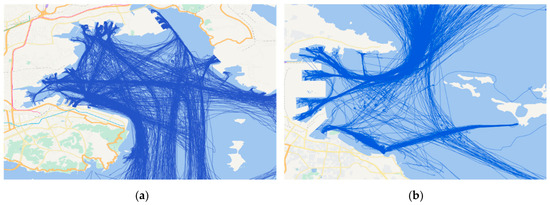
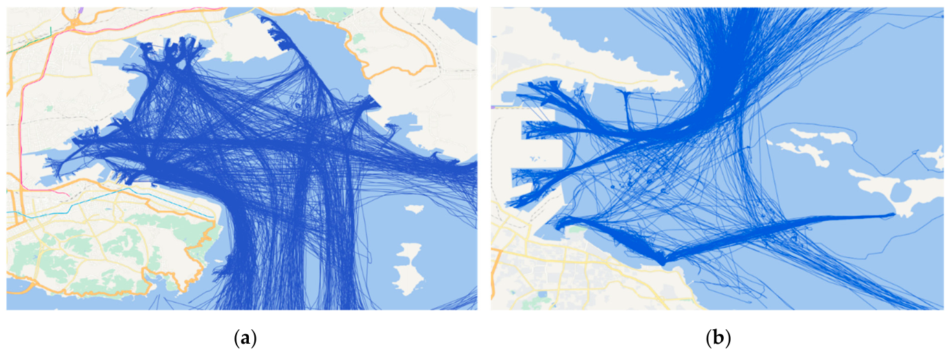
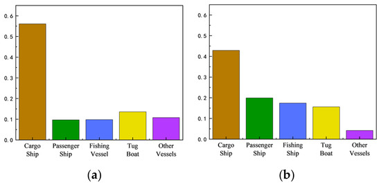
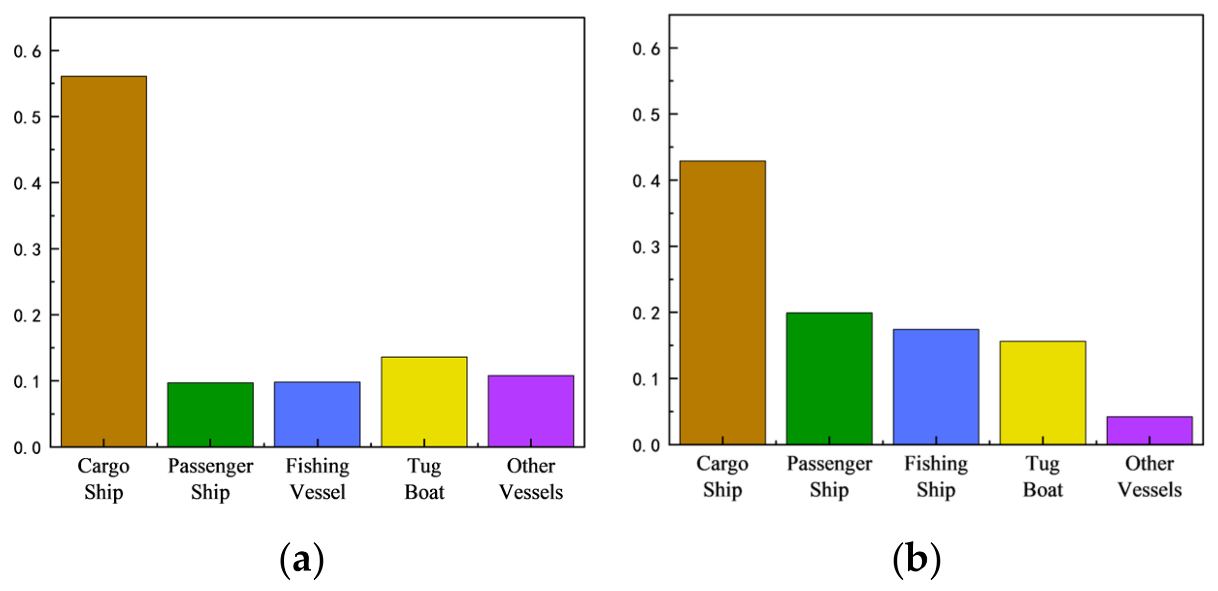
The experimental data utilized in this study comprises AIS records from Dalian Port and Yantai Port in June 2019. Dataset 1 covers the Dalian Port waters (121.60° E–121.86° E, 38.83° N–39.03° N) and contains 936 valid trajectories after preprocessing. Dataset 2 covers the area of Yantai Port (121.37° E–121.52° E, 37.51° N–37.61° N), with 832 valid trajectories, and is used specifically to evaluate the cross-port generalizability of the proposed model. Both datasets include various ship types, such as cargo ships, fishing vessels, and passenger ships. Their spatial distribution is shown in Figure 6, and the ship type distribution is shown in Figure 7.

Figure 6. Example of the experimental dataset. (a) Dalian Port dataset; (b) Yantai Port dataset.

Figure 7. Distribution of ship types in the experimental data. (a) Dalian Port ship type distribution; (b) Yantai Port ship type distribution.

3.1.2. Evaluation Metrics

The experiment adopts two commonly used indicators in the industry to quantitatively evaluate the quality of clustering results [31], as follows:

First, the Silhouette Score (SC) is selected to measure the intra-cluster compactness and inter-cluster separation, with a value range of [−1, 1]. The closer to 1, the more accurate the clustering effect. The calculation formula is shown in Equation (19), where SC is the Silhouette Score, T_i is the ship trajectory, n is the total number of trajectories, p(T_i) is the average distance from the i-th ship trajectory to all other ship trajectories in its cluster, and q(T_i) is the average distance from the i-th ship trajectory to the nearest cluster among all other clusters.

$$SC={\displaystyle \frac{1}{n}}{\displaystyle \sum _{i=1}^n\frac{q(T_i)-p(T_i)}{\max \left\{p(T_i),q(T_i)\right\}}}$$

(20)

The Davies–Bouldin Index (DBI) is selected to measure the similarity between clusters, with a value ≥0. The smaller the value, the more significant the difference between clusters. The calculation formula is:

$$DBI={\displaystyle \frac{1}{k}}{\displaystyle \sum _{i=1}^k{\max }_{j\ne i}}\left({\displaystyle \frac{S_i+S_j}{M_{ij}}}\right)$$

(21)

In Equation (21), k is the total number of clusters after ship trajectory clustering, Si is the average intra-cluster distance of the i-th cluster, and M_ij is the centroid distance between the i-th cluster and the j-th cluster.

3.1.3. Determination of Behavior Judgment Thresholds

This section defines the core thresholds in ship behavior recognition. Considering that the experimental area is port water with complex navigable ship types, to ensure the unity of the judgment standard and international comparability, the threshold setting refers to the relevant standards issued by IMO, IEC and ISO and is empirically set in combination with the application requirements of AIS trajectory behavior recognition in port scenarios. Referring to [32], the reporting frequency of dynamic information of ships in low speed or anchored/moored state is significantly different from that in normal navigation state. Therefore, this paper takes 0.5 kn as the recognition threshold for the stopped state and 3 kn as the division threshold for the slow speed navigation state.

For turning behavior, Referring to [33], the 10°/10° zig-zag test adopts a 10° heading deviation as the typical maneuverability test condition, indicating that the heading change of this magnitude is representative in ship maneuvering analysis. Therefore, this paper takes 10° as the empirical threshold to distinguish straight-line navigation from obvious turning behavior. For the severity of turning, ISO 20672:2022 involves a typical turning angular velocity test range, such as ±30°/min [34], indicating that this magnitude has engineering significance in ship turning monitoring. Therefore, this paper further takes 30°/min (0.5°/s) as the empirical threshold to distinguish steady turning from sharp turning. Reference [35] takes 0.1 kn/s as the extraction threshold of speed feature points, and this paper uses this value as the judgment standard for ship acceleration and deceleration.

3.2. Verification of Method Effectiveness and Generalization

3.2.1. Results of Dalian Port Dataset

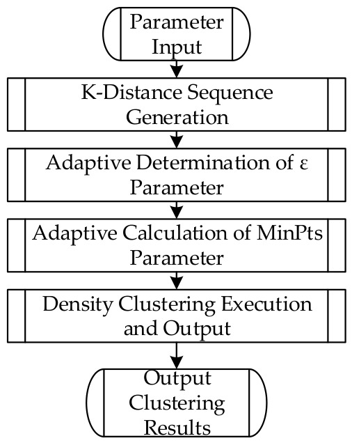
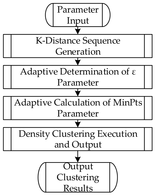
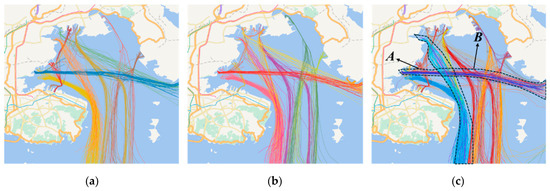
The core adjustable parameters of the proposed method are the weight of spatial distance and the weight of behavior distance. To accurately find the optimal weight combination, a grid search strategy is adopted with the goal of maximizing the clustering Silhouette Score. The weight search range is 0–1, with a step size of 0.1. The optimal parameter combination is obtained as the behavior weight of 0.3 and the spatial position weight of 0.7. The K_max is set to 10 to balance computational efficiency and density sensitivity, and the self-attenuation coefficient λ is set to 0.4 based on pre-experimental validation on both port datasets. On this basis, through the proposed adaptive parameter optimization mechanism, the final clustering parameters of the proposed method are determined as ε = 0.09 and MinPts = 5. The clustering result of the proposed method is shown in Figure 8c, and all trajectories are clustered into 28 clusters.

Figure 8. Comparison of clustering results of different methods in Dalian Port Dataset (a) Clustering result of classical DBSCAN; (b) clustering result of MD-DBTCAN; (c) clustering result considering navigation behavior.

To verify the effectiveness of the proposed method, the classical trajectory clustering method (DBSCAN) and the multi-dimensional ship trajectory clustering method based on the fusion distance metric (MD-DBTCAN) proposed in Reference [21] are selected as comparison methods. The adaptive mechanism is also used to determine the clustering parameters of the comparison methods. The clustering parameters of the classical DBSCAN are ε = 0.13 and MinPts = 6, and the clustering parameters of MD-DBTCAN are ε = 0.17 and MinPts = 3. The comparison of clustering result parameters of each method is shown in Table 3, and the schematic diagram of clustering results is shown in Figure 8.

Table 3. Comparison of clustering result parameters of different methods.

Method	Silhouette Score	DBI Index	Noise Rate	Clustering Parameters
Classical DBSCAN	0.45	0.66	23.67%	ε = 0.13 MinPts = 6
MD-DBTCAN	0.47	0.60	21.36%	ε = 0.17 MinPts = 3
Proposed Method	0.52	0.56	17.12%	ε = 0.09 MinPts = 5

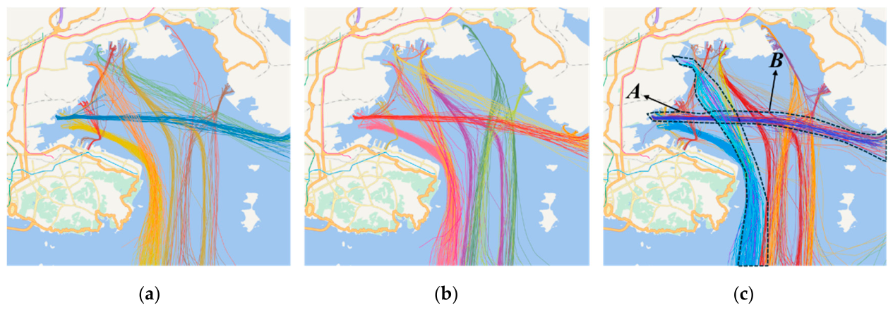
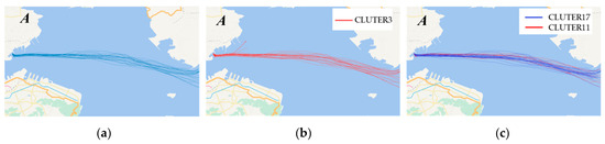
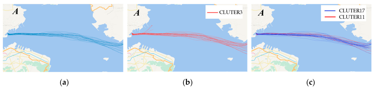
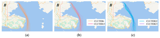
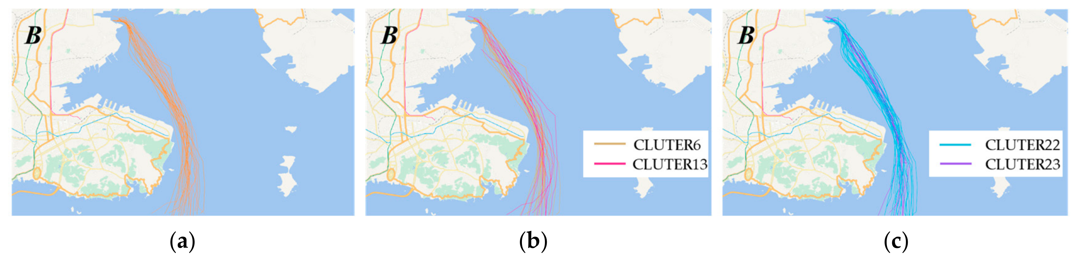
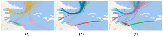
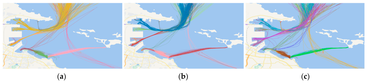
Table 3 shows that the proposed method outperforms the comparison methods across all metrics. The Silhouette Score is 0.52, which is 0.07 and 0.05 higher than the classical DBSCAN and MD-DBTCAN methods respectively. The DBI index of the proposed method is reduced to 0.56, which is 0.10 and 0.04 lower than the two comparison methods respectively. The Noise Rate is 17.12%, which is 6.55% and 4.24% lower than the two comparison methods respectively. This is because classical DBSCAN only uses spatial position features for clustering and cannot distinguish trajectories that overlap spatially but have different motion patterns. Although MD-DBTCAN introduces heading and speed features, it adopts the method of equal weight fusion after single-dimensional calculation, which is difficult to achieve clear separation between clusters. At the same time, in Figure 8c, the proposed method divides more clusters in Area A and Area B than the two comparison methods. For further analysis, the clustering results of the three methods in Area A and Area B are extracted for visual comparison, as shown in Figure 9 and Figure 10.

Figure 9. Comparison of clustering results of different methods in Area A. (a) Clustering result of classical DBSCAN; (b) clustering result of MD-DBTCAN; (c) clustering result considering navigation behavior.

Figure 10. Comparison of clustering results of different methods in Area B. (a) Clustering result of classical DBSCAN; (b) clustering result of MD-DBTCAN; (c) clustering result considering navigation behavior.

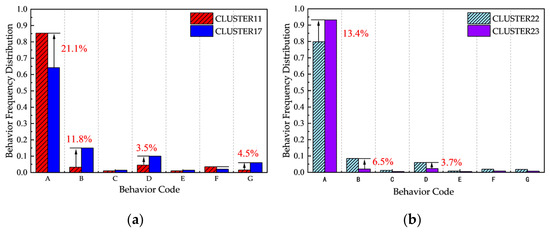
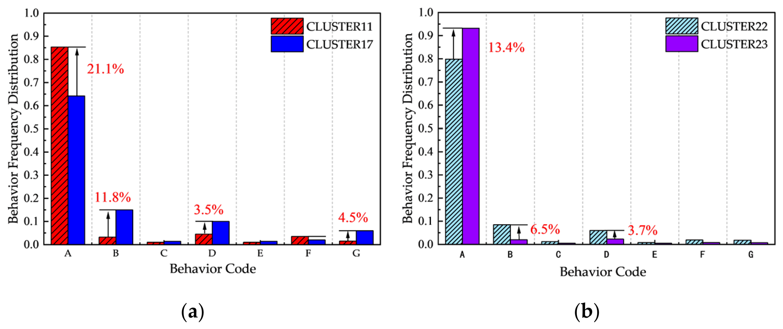
In Figure 9 and Figure 10, the proposed method divides the ship trajectories in Area A and Area B into two different clusters, the classical DBSCAN method classifies them into one cluster, and the MD-DBTCAN method can distinguish different clusters in Area B but clusters the ship trajectories into one category in the straight channel Area A without division. Further, the trajectories in these two areas are numerically analyzed, and the behavior frequency distribution of each cluster is counted, as shown in Figure 11.

Figure 11. Comparison of behavior frequency distribution of each cluster in Area A and Area B. (a) Comparison of behavior distribution frequency between Cluster 11 and Cluster 17 in Area A; (b) comparison of behavior distribution frequency between Cluster 22 and Cluster 23 in Area B.

It can be seen in Figure 11 that there are great differences in the behavior frequency distribution between the two clusters in Area A and Area B. Taking the normal navigation with the highest proportion as an example, the frequency of behavior A of Cluster 11 in Area A is 21.1% different from that of Cluster 17, and the frequency of behavior A of Cluster 22 in Area B is 13.4% different from that of Cluster 23. Therefore, the proposed method can divide the trajectories in these two areas into different clusters.

To explore the reason why the MD-DBTCAN method can achieve effective clustering in Area B but cannot complete effective division in the straight channel Area A, the Silhouette Scores of the clustering results in the two areas are calculated based on motion parameters and behavior sequences respectively, and the comparison results are shown in Table 4.

Table 4. Comparison of Silhouette Scores of clustering results of different methods in Area A and Area B.

Silhouette Score	Area A		Area B
	Proposed Method	MD-DBTCAN Method	Proposed Method	MD-DBTCAN Method
Based on Motion Parameters	0.37	-	0.45	0.62
Based on Behavior Sequence	0.65	-	0.67	0.51

Table 4 shows that, in Area B, the Silhouette Scores calculated based on motion parameters and behavior sequences are relatively close, indicating that the motion parameters and navigation behaviors of the trajectories in this area have certain differences, which is the reason why both the proposed method and the MD-DBTCAN method can achieve trajectory division in this area. In the straight channel Area A, all trajectories are clustered into one category by the MD-DBTCAN method, so the Silhouette Score is not calculated; the Silhouette Score of the clustering results of the proposed method is 0.37 based on motion parameters and reaches 0.65 based on behavior sequence. This result shows that the motion parameters of the trajectories in Area A are relatively similar, so the MD-DBTCAN method that only relies on motion parameters cannot achieve effective cluster division. At the same time, Figure 11a shows that, in the results of the proposed method, Cluster 11 is the trajectory with a high proportion of normal navigation state, while the proportion of acceleration state and slow speed state of Cluster 17 is 4.5% and 11.8% higher than that of Cluster 11 respectively. Therefore, the trajectories in this area have great differences in navigation behaviors, such as acceleration and deceleration, and the proposed method can effectively identify the trajectories with differences in such behaviors by measuring the edit distance of the behavior sequence and realize the effective division of the trajectories in this area.

3.2.2. Results of Yantai Port Dataset

To verify the scenario generalization ability of the method, a completely consistent comparative experiment is carried out on the Yantai Port dataset. Judged by the adaptive mechanism, the optimal clustering parameters of the proposed method are ε = 0.07 and MinPts = 5, and the 832 trajectories are finally clustered into 24 clusters. The schematic diagrams of clustering results of each method are shown in Figure 12, and the comparison of clustering performance is shown in Table 5.

Figure 12. Comparison of clustering results of different methods in Yantai Port Dataset. (a) Clustering result of classical DBSCAN; (b) clustering result of MD-DBTCAN; (c) clustering result considering navigation behavior.

Table 5. Comparison of clustering result parameters of different methods in Yantai Port dataset.

Method	Silhouette Score	DBI Index	Noise Rate	Clustering Parameters
Classical DBSCAN	0.41	0.78	27.36%	ε = 0.13 MinPts = 6
MD-DBTCAN	0.46	0.69	26.14%	ε = 0.17 MinPts = 3
Proposed Method	0.50	0.65	23.21%	ε = 0.07 MinPts = 5

It can be seen from the data in Table 5 that, on the Yantai Port dataset with more passenger ships and concentrated wharf distribution, the proposed method still maintains the optimal clustering performance. Its SC is 0.09 higher than that of the classical DBSCAN and 0.04 higher than that of the MD-DBTCAN method, and its DBI is 0.13 lower than that of the classical DBSCAN and 0.04 lower than that of the MD-DBTCAN method. Its Noise Rate is 4.35% and 2.93% lower than the two comparison methods. Combined with the experimental results on the Dalian Port dataset in Section 3.2.1, the core indicators of the proposed method perform similarly in the two scenarios, indicating that the method has stable performance in different scenarios and certain generalization ability.

3.3. Supplementary Experiments and Robustness Analysis

3.3.1. Sensitivity Analysis of Behavior Classification Thresholds and Weight Combination

1.

Sensitivity Analysis of Behavior Classification Thresholds;

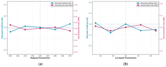
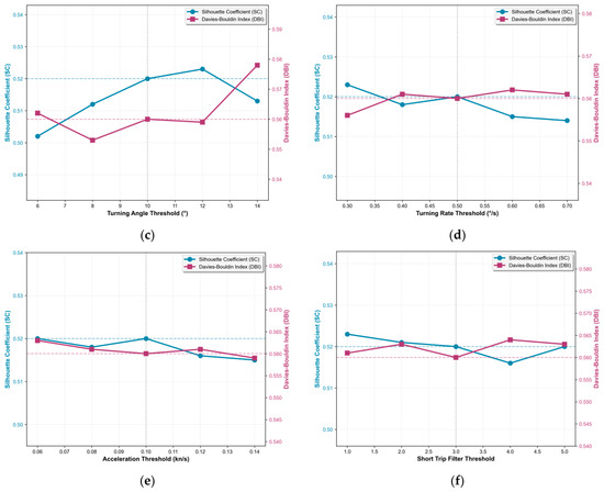
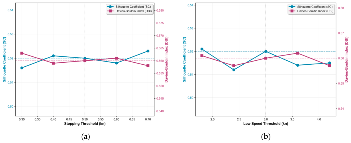
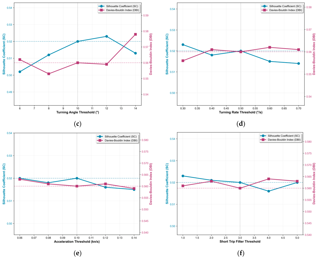
To verify the robustness of the proposed method against behavior classification thresholds, a control-variable method is used to perform sensitivity analysis on six core thresholds. Only one threshold is adjusted at each step, while all other parameters are fixed at baseline values. Five gradients are set within the range of ±40% of the baseline value, and the changes in SC and DBI of the proposed method on the Dalian Port dataset under different values are statistically analyzed. The value of behavior classification thresholds are shown in Table 6, and the variations are shown in Figure 13.

Table 6. Value of behavior classification thresholds.

Core Thresholds	Baseline Value	Value Gradients
Stopping Speed Threshold (kn)	0.5	0.3, 0.4, 0.5, 0.6, 0.7
Slow Speed Threshold (kn)	3.0	1.8, 2.4, 3.0, 3.6, 4.2
Turning Angle Threshold (°)	10.0	6.0, 8.0, 10.0, 12.0, 14.0
ROT Threshold (°/s)	0.5	0.3, 0.4, 0.5, 0.6, 0.7
Acceleration Threshold (kn/s)	0.1	0.06, 0.08, 0.1, 0.12, 0.14
Short Trip Filter Threshold	3	1, 2, 3, 4, 5

Figure 13. Variation in behavior classification thresholds. (a) Stopping speed threshold variation diagram; (b) slow speed threshold variation diagram; (c) turning angle threshold variation diagram; (d) ROT threshold variation diagram; (e) acceleration threshold variation diagram; (f) short trip filter threshold variation diagram.

As shown in Figure 13, when all core thresholds vary within ±40% of their baseline values, the SC values of the proposed method remain above 0.50, and the DBI values remain below 0.58, suggesting that the method is relatively insensitive to threshold fluctuations within the tested range and shows good robustness. It is worth noting that, as shown in Figure 13c, compared with the relatively flat curves when other parameters change, the fluctuations of the turning angle threshold cause relatively more significant changes in SC and DBI indicators. This is mainly because the turning angle is a key feature defining the core maneuvering behaviors of ships (straight navigation/turning), and its threshold change will directly affect the encoding of behavior sequences. Nevertheless, all results (SC > 0.50, DBI < 0.58) are still concentrated in the high-performance range. Considering all subfigures together, the proposed method maintains relatively stable performance when the core thresholds fluctuate within ±40%, indicating satisfactory robustness to moderate threshold perturbations.

2.

Sensitivity Analysis of Weight Combination;

The optimal weight combination was determined exclusively on the Dalian Port training dataset via grid search to maximize the Silhouette Score (SC), which is a standard model selection procedure for unsupervised clustering.

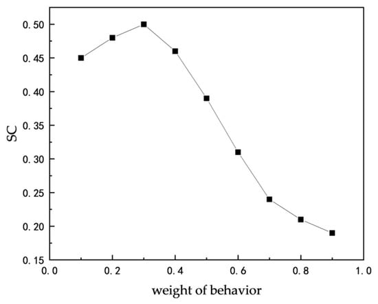
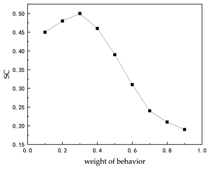
To evaluate the sensitivity of the proposed method to behavior weight, we fixed all other parameters and validated the clustering performance on the independent Yantai Port test dataset, with w_b varying from 0.1 to 0.9 with a step of 0.1. The variation is shown in Figure 14.

Figure 14. Variation in weight combination.

As shown in Figure 14, the results show that the fixed weight combination (w_b = 0.3, w_S = 0.7) derived from Dalian Port also achieves the optimal performance on Yantai Port. Moreover, the performance is relatively stable, and the SC value remains above 0.45 when w_b fluctuates between 0.2 and 0.4.

3.3.2. Ablation Experiments of Core Modules

To further isolate the contributions of the core designs in this paper, ablation analysis is conducted on behavior modeling, RLE, logarithmic normalization, and adaptive parameter selection while keeping the dataset, preprocessing process, spatial distance definition, and evaluation metrics consistent. It should be noted that behavior modeling (converting original trajectories into behavior sequences) is the fundamental improvement of this method. Removing this module will lead to the failure of the method, so its contribution is evaluated through the overall comparison between the full method and the baseline method. A total of one baseline group, three ablation groups, and one full method group are set up. Using the control variable method, only one core module is removed each time, and the remaining modules are completely consistent with the full method. Experiments are carried out on the Dalian Port dataset to quantify the contribution degree of each module through performance changes. To ensure experimental fairness, the classical DBSCAN in the baseline group and the full method of this paper adopt the same adaptive parameter determination mechanism to eliminate the interference of parameter selection differences on the experimental results.

The group settings and experimental results of the ablation experiments are shown in Table 7.

Table 7. Ablation experiment settings and results.

Group No.	Group Setting	SC	DBI
Baseline Group	Classical DBSCAN (with the same adaptive parameter mechanism, clustering only based on spatial coordinates)	0.45	0.66
Ablation Group 1	Remove RLE compression and calculate edit distance directly on the original behavior sequences	0.51	0.60
Ablation Group 2	Perform RLE compression and replace logarithmic mapping with linear normalization	0.51	0.58
Ablation Group 3	Cancel adaptive optimization and adopt the traditional fixed parameter strategy	0.52	0.57
Full Method Group	The complete method of this paper with all modules retained	0.52	0.56

The results of Table 7 show that the complete method in this article achieves the best clustering effect, and the performance of all melting groups is not better than that of the complete method, which indicates that there is a positive contribution to the design of each module. The analysis of each module is as follows.

Behavior modeling is the primary source of performance improvement in this work. Compared with the baseline group without behavior modeling, the SC value of the full method increases by 0.07, and the DBI value decreases by 0.10, achieving the most significant optimization of clustering effect.

RLE is a core auxiliary module. After removing RLE compression, the SC value of the method decreases by 0.01, and the DBI value increases by 0.04, resulting in a decline in clustering performance. On the other hand, this module reduces the time complexity of edit distance from O(n × m) for the original point-by-point sequences (where n and m are the number of original sampling points of two trajectories) to O(L₁ × L₂) at the behavior segment level (where L₁ and L₂ are the number of behavior segments of two trajectories), thus reducing the computational overhead.

After replacing logarithmic normalization with linear normalization, the SC value of the method decreases by 0.01, and the DBI value increases by 0.02, resulting in a slight decrease in clustering performance. This module mainly solves the problem that linear normalization is sensitive to extreme values of ship behavior features such as speed and turning angle and ensures the balanced contribution of different behavior features to similarity calculation.

Adaptive parameter optimization is the least contributing general auxiliary module. After changing to the fixed parameter strategy, the SC value of the method did not change; only the DBI value increased slightly by 0.01, which had the least impact on the core cluster performance. For the fixed-parameter ablation, ε = 0.08 and MinPts = 4 were selected from preliminary tuning and then kept constant across all ablation settings. The adaptive parameter mechanism mainly eliminates the subjectivity of manual tuning and ensures stable performance across different datasets, while the main source of performance improvement of this method is the behavior modeling and sequence similarity measurement framework.

3.3.3. Analysis of Algorithm Computational Complexity and Running Efficiency

1.

Theoretical Time Complexity Analysis;

The proposed method is divided into three core stages, and the time complexity analysis of each stage is as follows:

(1)

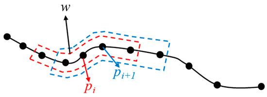
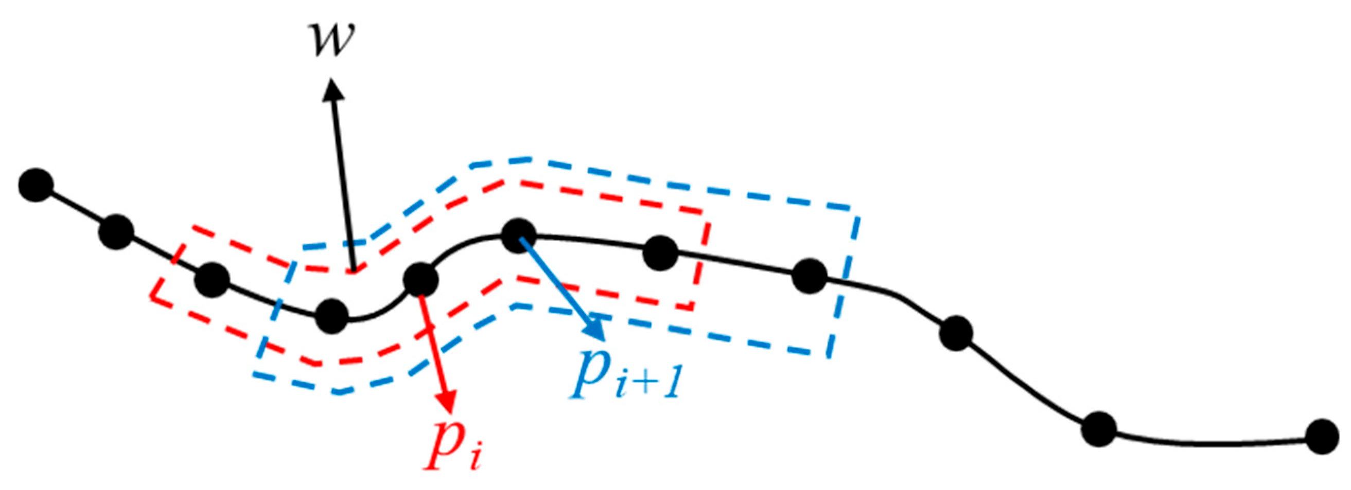
Key Motion Parameter Calculation Stage: Let the total number of trajectories be N, the average number of points per trajectory be L, and the average size of the sliding window be w. In this paper, the window size is adaptively determined with the trajectory length, i.e., w = O($\surd L$). The computational complexity within the window for each trajectory point is O(w), so the total complexity of this stage is O(N·L·w) = O(N·L^1.5). To prevent the window from being too large, the window size in the Formula (1) is limited to 11, and the computation per point is restricted to a constant amount, so the complexity of this stage is actually O(N·L).

(2)

Distance Measurement Stage: For spatial distance, the computational complexity of the Hausdorff distance between two trajectories is O(L₁·L₂), and the total complexity for all trajectory pairs is O(N²·L²), which is consistent with the classical DBSCAN and MD-DBTCAN methods. For behavior distance, after RLE compression, the average length of behavior sequences M ≪ L, the computational complexity of weighted edit distance between two sequences is O(M²), and the total complexity is O(N²·M²), which is negligible compared with spatial distance calculation. Therefore, the total complexity of this stage is O(N²·L²), which is in the same order of magnitude as classical DBSCAN.

(3)

Adaptive DBSCAN Clustering Stage: The time complexity of classical DBSCAN is O(N²). The complexity of the adaptive parameter optimization process in this paper is O(K_max·N²), where K_max is a fixed small value (set to 10 in this paper). Therefore, the total complexity of this stage is O(N²).

2.

Actual Running Efficiency Comparison;

All experiments are completed in a unified hardware environment with the following specific configuration: CPU is AMD Ryzen9 9955HX made in China, memory is 32 GB, operating system is Windows 11. The algorithm is implemented based on Python 3.8, where the spatial distance calculation is implemented based on the Geopy library, and the clustering algorithm is extended based on the Scikit-learn library.

On the Dalian Port dataset, the total end-to-end running time of the three methods is statistically analyzed, and the running time changes under different numbers of trajectories are tested to verify the scalability of the method. The results are shown in Table 8.

Table 8. Comparison of running time of different methods (Unit: s).

Method	Dalian Port Dataset (936 Trajectories)	Yantai Port Dataset (832 Trajectories)	2000 Trajectories
Classical DBSCAN	88.2	81.2	330.1
MD-DBTCAN	123.3	115.6	530.3
Proposed Method	95.1	86.1	342.2

It can be seen in Table 8 that, on the two experimental datasets, the total running time of the proposed method increases by 4.9–6.9 s compared with classical DBSCAN, with relative increases in computational overhead of approximately 7.8% and 6.0% respectively. Meanwhile, it is 28.2–29.5 s less than the MD-DBTCAN method. The reason is that the MD-DBTCAN method calculates the fusion distances of position, heading, and speed separately and then weights them, with a computational complexity of O(N²·L²). Although all three methods belong to the quadratic order of magnitude, MD-DBTCAN has a larger constant factor because it needs to calculate three attribute distances separately and fuse them, leading to increased computation time.

With the increase in the number of trajectories, the growth rate of running time of the proposed method is basically consistent with the two comparison methods. At the scale of 2000 trajectories, the computation time increases by 12.1 s compared with classical DBSCAN while still maintaining acceptable running efficiency. This indicates that the proposed method remains computationally practical for the tested trajectory scale.

3.3.4. Statistical Significance Analysis and Robustness Verification

Although the experimental results in Section 3.2 show that the proposed method generally outperforms the comparison methods in both SC and DBI, given the inherent randomness of clustering algorithms and evaluation processes, the differences in single evaluations may be within the range of random fluctuations. To strictly verify the statistical significance of the performance improvement of the proposed method and evaluate the stability of its results, this section adopts Bootstrap resampling and statistical hypothesis testing for quantitative analysis.

The specific evaluation process for the Dalian Port dataset is as follows:

(1)

Perform 100 rounds of random resampling with replacement on the original dataset, generating a Bootstrap sample of the same size as the original dataset each time. This process aims to obtain the approximate sampling distribution of performance indicators by simulating multiple independent samplings.

(2)

Run the proposed method and comparison methods independently on each Bootstrap sample and record their SC and DBI values. Finally, 100 sets of performance indicators are obtained for each method.

(3)

Statistical Test: Due to the dependence between Bootstrap samples and the unknown distribution of performance indicators, the non-parametric paired Wilcoxon signed-rank test is adopted. We test SC and DBI separately: the null hypothesis (H0) is that there is no difference in the median of a certain indicator between the two methods; the alternative hypothesis (H1) is that the median of the proposed method on this indicator is significantly better (i.e., higher SC or lower DBI). The significance level is set to 0.05.

Table 9 shows the detailed statistical test results on the Dalian Port dataset.

Table 9. Statistical test results of Dalian Port dataset.

Comparison Method (Baseline)	Evaluation Metric	Proposed Method (Median ± IQR)	Comparison Method (Median ± IQR)
Classical DBSCAN	SC	0.518 (0.511, 0.523)	0.447 (0.443, 0.450)
Classical DBSCAN	DBI	0.558 (0.550, 0.567)	0.661 (0.655, 0.668)
MD-DBTCAN	SC	0.518 (0.511, 0.523)	0.466 (0.461, 0.471)
MD-DBTCAN	DBI	0.558 (0.550, 0.567)	0.602 (0.597, 0.611)

Note: IQR is the interquartile range, which reflects the fluctuation range of the results. The p-values are obtained from the one-tailed paired Wilcoxon signed-rank test.

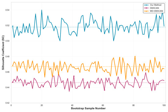
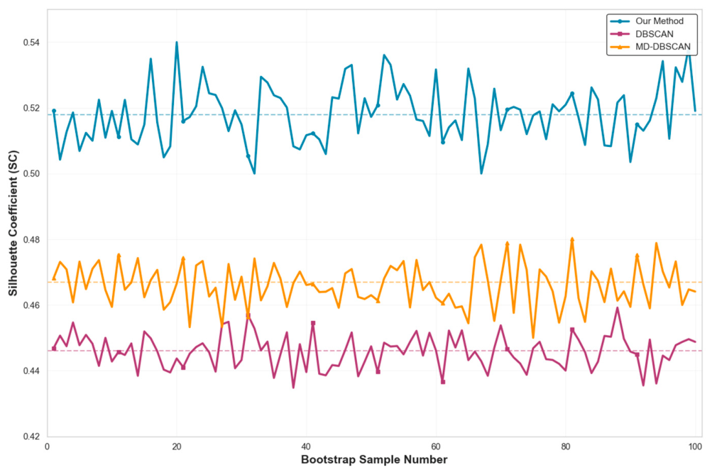
For a more intuitive presentation, Figure 14 plots the paired difference distribution of SC scores between the proposed method and the two comparison methods in 100 resampling.

It can be seen in Table 9 that the p-values in all comparison scenarios are far below 0.001; therefore, the null hypothesis can be rejected at the α = 0.05 significance level. This indicates that the observed performance improvements of the proposed method over the baseline methods are statistically significant under the current resampling setting. Meanwhile, Figure 15 shows that, across all 100 resampling runs, the proposed method yields uniformly better SC differences relative to the baseline methods.

Figure 15. SC difference distribution between the proposed method and comparison methods (Dalian Port dataset, 100 resampling).

4. Conclusions

This paper proposes a ship trajectory clustering method considering navigation behavior. Through analysis and experimental validation, the main conclusions are as follows:

(1)

The Silhouette Score of the clustering results of the proposed method is 0.07 and 0.05 higher than that of the classical DBSCAN and MD-DBTCAN methods, and the DBI index is reduced by 0.10 and 0.04 respectively. Thus, the clustering results suggest improved inter-cluster discrimination and a finer clustering granularity.

(2)

Compared with the classical DBSCAN method, the proposed method can effectively split the heterogeneous trajectories mis-clustered by classical DBSCAN in experimental Areas A and B. The maximum difference in the frequency of normal straight-line navigation behavior between the two clusters after splitting reaches 21.1%, which suggests that the method can better capture differences in turning behavior. Compared with the MD-DBTCAN method, in the straight channel Area A, the frequency of acceleration behavior and slow speed behavior of the two types of trajectories divided by the proposed method differs by 4.5% and 11.8% respectively, while MD-DBTCAN cannot achieve effective division because it cannot capture such fine-grained behavior differences.

(3)

The generalization experiments on the independent Yantai Port dataset show that the proposed method maintains stable performance across two typical northern Chinese port scenarios, providing preliminary evidence of its cross-port applicability. The sensitivity analysis supports the robustness of the method to fluctuate in core thresholds, the ablation experiments highlight the contributions of the core modules, and the complexity analysis indicates its practical scalability.

Nevertheless, the proposed method has several limitations that require further investigation. It only considers basic navigational behaviors, such as steady turning, emergency turning, and ship acceleration and deceleration, but has not yet considered complex navigational behaviors; at the same time, behavior classification thresholds and weights use globally fixed values and do not account for maneuverability differences between ship types, such as cargo ships, fishing vessels, and passenger ships. Additionally, this study evaluates clustering performance using internal validation metrics and does not conduct in-depth analysis of the navigation behavior patterns within individual clusters.

In the future, we will expand the ship navigation behavior classification system by introducing complex navigation behaviors such as collision avoidance, anchoring operations, and towing operations; we will study determining ship behavior thresholds and behavior weights through adaptive mechanisms and adjust behavior judgment thresholds according to the maneuvering characteristics of different ships to improve the accuracy of behavior classification. We will incorporate expert-validated route data to further verify the operational significance of the clustering results and analyze the typical behavior characteristics of each cluster. In addition, we will further explore deep learning methods and graph theory methods in ship behavior extraction and trajectory clustering to improve the accuracy of ship behavior recognition.

References

- Huang, I.-L.; Lee, M.-C.; Chang, L.; Huang, J.-C. Development and Application of an Advanced Automatic Identification System (AIS)-Based Ship Trajectory Extraction Framework for Maritime Traffic Analysis. J. Mar. Sci. Eng. 2024, 12, 1672. [Google Scholar] [CrossRef] [Scilit]
- Yang, D.; Wu, L.; Wang, S.; Jia, H.; Li, K.X. How Big Data Enriches Maritime Research—A Critical Review of Automatic Identification System (AIS) Data Applications. Transp. Rev. 2019, 39, 755–773. [Google Scholar] [CrossRef] [Scilit]
- Li, H.; Lam, J.S.L.; Yang, Z.; Liu, J.; Liu, R.W.; Liang, M.; Li, Y. Unsupervised Hierarchical Methodology of Maritime Traffic Pattern Extraction for Knowledge Discovery. Transp. Res. Part C Emerg. Technol. 2022, 143, 103856. [Google Scholar] [CrossRef] [Scilit]
- Hu, X.; Xie, L.; Chang, J.; Yang, Y.; Ou, C. Application of improved QuickBundles algorithm in ship trajectory clustering. Navig. China 2023, 46, 145–152. [Google Scholar] [CrossRef]
- MacQueen, J.B. Some Methods for Classification and Analysis of Multivariate Observations. In Proceedings of the Fifth Berkeley Symposium on Mathematical Statistics and Probability; University of California Press: Berkeley, CA, USA, 1967; Volume 1, pp. 281–297. [Google Scholar]
- Mieczyńska, M.; Czarnowski, I. K-Means Clustering for SAT-AIS Data Analysis. WMU J. Marit. Aff. 2021, 20, 377–400. [Google Scholar] [CrossRef] [Scilit]
- Zhen, R.; Jin, Y.; Hu, Q.; Shao, Z.; Nikitakos, N. Maritime Anomaly Detection within Coastal Waters Based on Vessel Trajectory Clustering and Naïve Bayes Classifier. J. Navig. 2017, 70, 648–670. [Google Scholar] [CrossRef] [Scilit]
- Ester, M.; Kriegel, H.-P.; Sander, J.; Xu, X. A Density-Based Algorithm for Discovering Clusters in Large Spatial Databases with Noise. In Proceedings of the Second International Conference on Knowledge Discovery and Data Mining; AAAI Press: Portland, OR, USA, 1996; pp. 226–231. [Google Scholar]
- Sheng, P.; Yin, J. Extracting Shipping Route Patterns by Trajectory Clustering Model Based on Automatic Identification System Data. Sustainability 2018, 10, 2327. [Google Scholar] [CrossRef] [Scilit]
- Liu, Z.; Yang, H.; Xiong, C.; Xu, F.; Gan, L.; Yan, T.; Shu, Y. Research on the Optimization of Ship Trajectory Clustering Based on the OD–Hausdorff Distance. J. Mar. Sci. Eng. 2024, 12, 1398. [Google Scholar] [CrossRef] [Scilit]
- Zhang, C.; Liu, S.; Guo, M.; Liu, Y. A Novel Ship Trajectory Clustering Analysis and Anomaly Detection Method Based on AIS Data. Ocean Eng. 2023, 288, 116082. [Google Scholar] [CrossRef] [Scilit]
- Wang, L.; Chen, P.; Chen, L.; Mou, J. Ship AIS Trajectory Clustering: An HDBSCAN-Based Approach. J. Mar. Sci. Eng. 2021, 9, 566. [Google Scholar] [CrossRef] [Scilit]
- Shen, H.; Tang, H.; Yin, Y. A Novel Method for Ship Trajectory Clustering. Int. J. Nav. Archit. Ocean Eng. 2022, 14, 100474. [Google Scholar] [CrossRef] [Scilit]
- Xiong, L.; Xiong, X.; Zhang, F.; Chen, H. Unsupervised Deep Embedding Clustering for AIS Trajectory. In Proceedings of the IGARSS 2022—2022 IEEE International Geoscience and Remote Sensing Symposium; IEEE: Kuala Lumpur, Malaysia, 2022; pp. 2283–2286. [Google Scholar]
- Murray, B.; Perera, L.P. Deep Representation Learning-Based Vessel Trajectory Clustering for Situation Awareness in Ship Navigation. In Developments in Maritime Technology and Engineering; CRC Press: London, UK, 2021; pp. 157–165. ISBN 978-1-003-21658-2. [Google Scholar]
- Abuella, M.; Atoui, M.A.; Nowaczyk, S.; Johansson, S.; Faghani, E. Spatial Clustering Approach for Vessel Path Identification. IEEE Access 2024, 12, 66248–66258. [Google Scholar] [CrossRef] [Scilit]
- Zhang, R.; Fan, Y.; Zhang, D. Vessel Trajectory Association Algorithm Based on Deep Learning Trajectory Similarity with Post-Processing. In Proceedings of the 2025 4th International Conference on Cyber Security, Artificial Intelligence and the Digital Economy; ACM: Kuala Lumpur, Malaysia, 2025; pp. 683–689. [Google Scholar]
- Baghizadeh, K.; Pahl, J.; Lützen, M.; Rytter, N.G.M. Using AIS Data to Analyze and Optimize Vessel Operations for Offshore Wind Farm Maintenance. In Proceedings of the Innovations in Sustainable Maritime Technology—IMAM 2025; Spyrou, K.J., Themelis, N., Eds.; Springer Nature: Cham, Switzerland, 2025; pp. 405–422. [Google Scholar]
- Xu, X.; Cui, D.; Li, Y.; Xiao, Y. Research on Ship Trajectory Extraction Based on Multi-Attribute DBSCAN Optimisation Algorithm. Pol. Marit. Res. 2021, 28, 136–148. [Google Scholar] [CrossRef] [Scilit]
- Liu, L.; Zhang, Y.; Hu, Y.; Wang, Y.; Sun, J.; Dong, X. A Hybrid-Clustering Model of Ship Trajectories for Maritime Traffic Patterns Analysis in Port Area. J. Mar. Sci. Eng. 2022, 10, 342. [Google Scholar] [CrossRef] [Scilit]
- An, J.; Li, H.; Lei, Y.; Wang, Y.; Yao, C. Mining Method of Ship Activity Trajectory Pattern Based on Big Data. Fire Control Command Control 2024, 49, 156–163. [Google Scholar] [CrossRef]
- Wen, Y.; Song, R.; Huang, L.; Huang, Y.; Sui, Z.; Zhu, M. Semantic Modeling and Expression for Ship Behaviors. J. Harbin Inst. Technol. 2021, 53, 109–115. [Google Scholar] [CrossRef]
- Lei, J.; Sun, Y.; Wu, Y.; Zheng, F.; He, W.; Liu, X. Association of AIS and Radar Data in Intelligent Navigation in Inland Waterways Based on Trajectory Characteristics. J. Mar. Sci. Eng. 2024, 12, 890. [Google Scholar] [CrossRef] [Scilit]
- Chen, X.; Ling, J.; Yang, Y.; Zheng, H.; Xiong, P.; Postolache, O.; Xiong, Y. Ship Trajectory Reconstruction from AIS Sensory Data via Data Quality Control and Prediction. Math. Probl. Eng. 2020, 2020, 7191296. [Google Scholar] [CrossRef] [Scilit]
- Zhang, L.; Zhu, Y.; Lu, W.; Wen, J.; Cui, J. A detection and restoration approach for vessel trajectory anomalies based on AIS. Xibei Gongye Daxue Xuebao/J. Northwest. Polytech. Univ. 2021, 39, 119–125. [Google Scholar] [CrossRef] [Scilit]
- Huang, L.; Wen, Y.; Guo, W.; Zhu, X.; Zhou, C.; Zhang, F.; Zhu, M. Mobility Pattern Analysis of Ship Trajectories Based on Semantic Transformation and Topic Model. Ocean Eng. 2020, 201, 107092. [Google Scholar] [CrossRef] [Scilit]
- Wu, S.; Zimányi, E.; Sakr, M.; Torp, K. Semantic Segmentation of AIS Trajectories for Detecting Complete Fishing Activities. In Proceedings of the 2022 23rd IEEE International Conference on Mobile Data Management (MDM); IEEE: New York, NY, USA, 2022; pp. 419–424. [Google Scholar]
- Wagner, R.A.; Fischer, M.J. The String-to-String Correction Problem. J. ACM 1974, 21, 168–173. [Google Scholar] [CrossRef] [Scilit]
- Taha, A.A.; Hanbury, A. An Efficient Algorithm for Calculating the Exact Hausdorff Distance. IEEE Trans. Pattern Anal. Mach. Intell. 2015, 37, 2153–2163. [Google Scholar] [CrossRef] [Scilit]
- Wan, J.; Hu, D.; Jiang, Y. Research on Method of Multi-density Self-Adaptive Determination of DBSCAN Algorithm Parame-ters. Comput. Eng. Appl. 2022, 58, 78–85. [Google Scholar] [CrossRef]
- Mou, F.; Fan, Z.; Li, X.; Wang, L.; Li, X. A Method for Clustering and Analyzing Vessel Sailing Routes Efficiently from AIS Data Using Traffic Density Images. J. Mar. Sci. Eng. 2023, 12, 75. [Google Scholar] [CrossRef] [Scilit]
- IEC 61993-2:2018; Maritime Navigation and Radiocommunication Equipment and Systems—Automatic Identification Systems (AIS)—Part 2: Class A Shipborne Equipment of the Automatic Identification System (AIS)—Operational and Performance Requirements, Methods of Test and Required Test Results. IEC: Geneva, Switzerland, 2018.
- Resolution MSC.137(76); Standards for Ship Manoeuvrability. IMO: London, UK, 2002.
- ISO 20672:2022; Ships and Marine Technology—Rate-of-Turn Indicators. ISO: Geneva, Switzerland, 2022.
- Zhang, B.; Hirayama, K.; Ren, H.; Wang, D.; Li, H. Ship Anomalous Behavior Detection Using Clustering and Deep Recurrent Neural Network. J. Mar. Sci. Eng. 2023, 11, 763. [Google Scholar] [CrossRef] [Scilit]
Disclaimer/Publisher’s Note: The statements, opinions and data contained in all publications are solely those of the individual author(s) and contributor(s) and not of MDPI and/or the editor(s). MDPI and/or the editor(s) disclaim responsibility for any injury to people or property resulting from any ideas, methods, instructions or products referred to in the content. |
© 2026 by the authors. Licensee MDPI, Basel, Switzerland. This article is an open access article distributed under the terms and conditions of the Creative Commons Attribution (CC BY) license.