Research on a Multi-Parameter Identification Method for Underwater Inductive Power Transfer Systems

Abstract

In underwater inductive power transfer (IPT) systems, the variation of eddy-current losses with frequency can degrade the accuracy of parameter identification. To address this issue, this paper proposes a multi-parameter identification method for a double-sided LCC system. First, based on the circuit model and the frequency dependence of the equivalent eddy-current loss resistance, six sets of equations are established, transforming the parameter identification problem into an optimization problem. Then, to balance global search capability and convergence speed, a hybrid particle swarm optimization algorithm is employed to identify the unknown parameters. Simulation and experimental results show that, under different coil spacings, load conditions, and medium conductivities, the proposed method can accurately identify key parameters, with the overall relative error controlled within 5%. This method is applicable to parameter monitoring and performance regulation of underwater IPT systems.

1. Introduction

Autonomous underwater vehicles (AUVs), characterized by high maneuverability and autonomy, have become key platforms for underwater exploration, monitoring, and resource development [1,2,3]. Wireless power transfer (WPT), with the advantages of non-contact operation, safety, reliability, and concealment, provides a new approach for supplying energy to AUVs [4,5,6,7,8]. Among various WPT technologies, inductive power transfer (IPT) has stood out because of its high power density and strong anti-interference capability in underwater environments [9,10,11,12].

To achieve precise regulation of IPT system performance, accurate information on the equivalent circuit parameters must be obtained. In conventional schemes, parameter acquisition usually relies on additional wireless communication modules installed on both the primary and secondary sides, such as Bluetooth or Wi-Fi modules [13,14]. However, this approach not only increases hardware complexity, volume, and cost but also is prone to communication failures in harsh underwater environments [15,16], thereby reducing overall system reliability. Therefore, parameter identification methods that do not depend on communication have become essential for dynamic monitoring of IPT system parameters. At present, existing parameter identification methods can generally be classified into three categories: auxiliary component based methods, non-resonant steady-state circuit methods, and frequency scanning methods.

Auxiliary, component-based methods were introduced in [17,18]. Their main idea is to incorporate additional auxiliary devices into the circuit, such as switched capacitors or switchable relay compensation capacitors so as to create different resonant frequency points or establish specific mathematical models. Parameter identification of the load and mutual inductance is then achieved under the corresponding operating conditions. Ref. [19] proposed a dual-mode switching identification method, in which an additional capacitor enables the system to operate in two distinct modes, and the load and mutual inductance are identified based on the resulting mathematical model. Ref. [20] adopted a dual-inverter modulation scheme in which the main and auxiliary inverters are connected in series on the transmitter side; by detecting the beat envelope characteristics of the transmitter coil current and combining them with predefined conditions, equations were established to identify the mutual inductance and load parameters. Although these methods can provide satisfactory identification performance, they require additional components to be introduced into the original circuit, which inevitably increases system complexity.

Non-resonant steady-state circuit methods identify unknown parameters by intentionally operating the IPT system away from resonance and then inferring the parameters from the steady-state circuit model and measurable electrical quantities. For the SS-IPT system, ref. [21] proposed a method for identifying mutual inductance and load parameters under non-resonant conditions. Specifically, the input impedance was calculated from the amplitude of the primary coil current and the phase difference between the inverter output voltage and the primary current, and the unknown parameters were then solved accordingly. Although such methods can identify parameters such as mutual inductance and load, they are only applicable to specific static conditions, and their applicability is limited in scenarios where the coupling conditions may vary.

Frequency scanning methods identify parameters by exploiting the variation of equivalent impedance with operating frequency. Refs. [22,23] showed that changes in mutual inductance, load, and frequency lead to different variations in the equivalent impedance seen from the primary side, making it possible to establish equations between the unknown parameters and the equivalent impedance. Ref. [24] further demonstrated that, in an SS-type IPT system, the impedance angle of the primary side equivalent impedance changes with frequency, and that the corresponding transition frequency is closely related to the coupling coefficient; therefore, the coupling coefficient can be determined accordingly. Ref. [25] established a mathematical model of the primary side equivalent impedance at multiple operating frequencies and employed an adaptive particle swarm optimization algorithm to identify parameters such as mutual inductance and load. This method features a simple structure and is capable of simultaneous identification of multiple parameters. However, in underwater IPT systems, eddy-current loss in seawater usually appears as an additional resistive loss, and its value changes with operating frequency [26,27,28,29]. If this frequency dependence is ignored in parameter identification, the identification accuracy will decrease. In [30], a frequency-scanning method combined with an ANN algorithm was used to identify the mutual inductance M and load resistance R_L. To reduce the influence of frequency, only small frequency variations are used, so the frequency dependence of system parameters is neglected. This method works well when only a few parameters need to be identified, because parameter decoupling is relatively easy. However, for multi-parameter identification, its decoupling ability is limited, which may reduce accuracy. To improve this problem, refs. [31,32,33] further consider the frequency-dependent eddy-current loss in underwater IPT systems, which improves the accuracy of multi-parameter identification. However, these methods require voltage and current phase measurements, making implementation difficult and increasing hardware requirements.

To address this issue, this paper adopts the frequency scanning method and incorporates the relationship between the equivalent resistance of eddy-current loss and frequency. Based on the equivalent circuit model, a four-variable equation set is constructed. By measuring the port voltage and current, the impedance magnitudes of Z_in1 and Z_in2 are obtained. Then, a hybrid particle swarm optimization algorithm is employed for parameter identification, transforming the determination of the unknown parameters into an objective function optimization problem and thereby enabling accurate identification of the unknown parameters. The remainder of this paper is organized as follows. Section 2 presents the system modeling and theoretical analysis. Section 3 presents the multi-parameter identification method based on the hybrid particle swarm optimization algorithm and provides simulation validation. Section 4 reports the experimental validation. Finally, Section 5 concludes the paper.

2. Modeling of Underwater DLCC-IPT System

2.1. Eddy-Current Loss Modeling and Frequency Dependence

In circuit modelling, the eddy-current effect is modeled by an equivalent resistance, which is appropriate for the low-frequency range considered here [27]. The inductive contribution of eddy currents becomes more relevant at higher frequencies [28] and is therefore neglected in the present model to keep the formulation concise. This assumption is valid for the operating conditions investigated in this work.

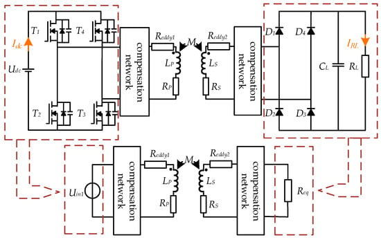
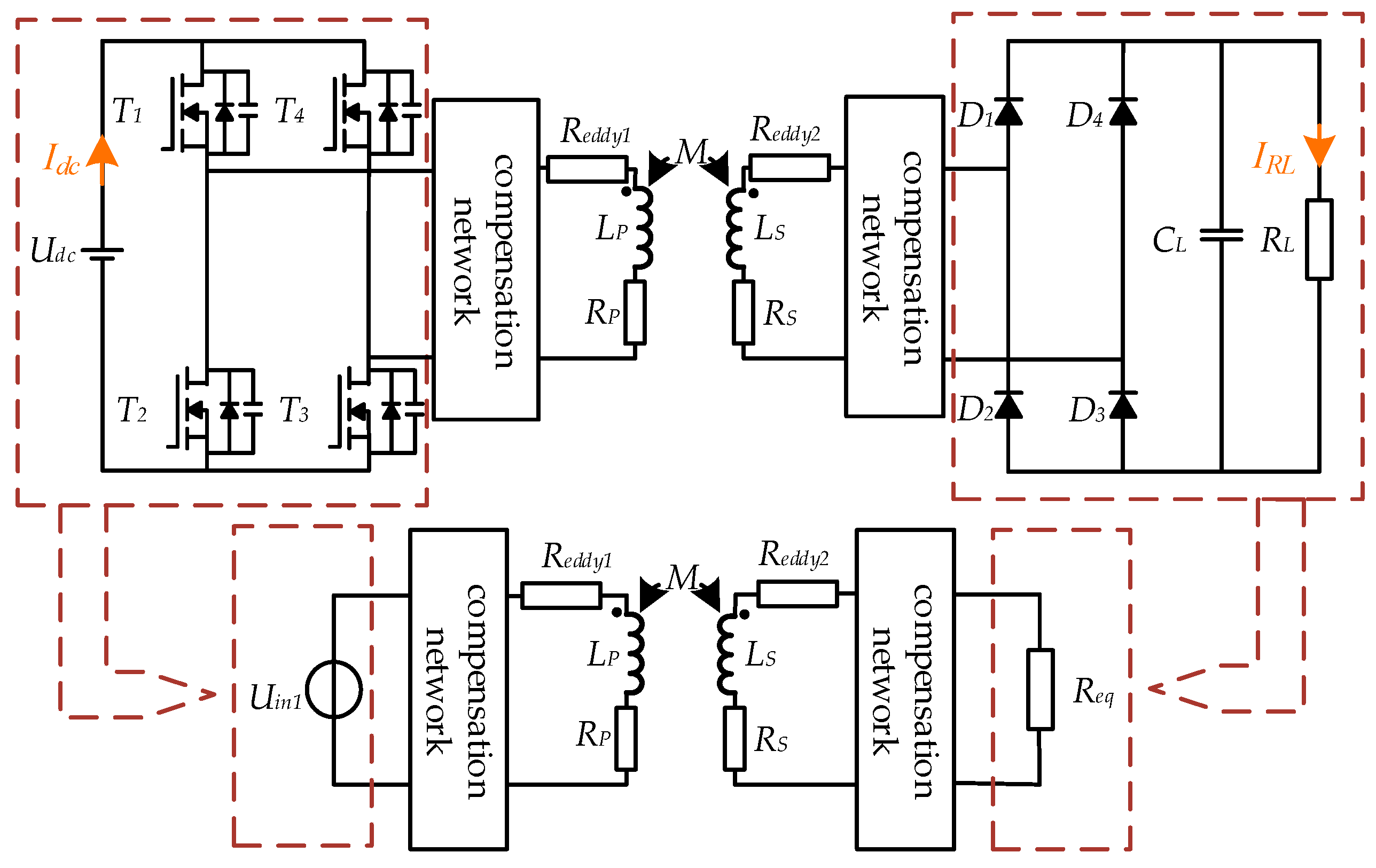
Figure 1 shows the equivalent circuit model of the IPT coils with eddy-current loss taken into account. Here, U_dc denotes the input DC voltage, and U_in1 is the inverter output voltage. R_p and R_S represent the parasitic resistances of inductors L_P and L_S, respectively. R_eddy1 and R_eddy2 are the equivalent resistances associated with eddy-current loss on the primary and secondary sides, respectively. M is the mutual inductance between the coils, while L_P and L_S are the primary and secondary side inductances. T₁–T₄ are MOSFETs, and D₁–D₄ are diodes. R_eq denotes the equivalent load, and R_L is the load. The relationships among R_eq, R_L, U_dc, and U_in1 are given in (1) and (2).

$$R_{eq}={\displaystyle \frac{8}{{\pi }^2}}{R}_L$$

(1)

$$U_{in1}={\displaystyle \frac{4}{\pi }}{U}_{dc}\sin (\omega t)$$

(2)

Figure 1. The equivalent circuit model of the IPT coils.

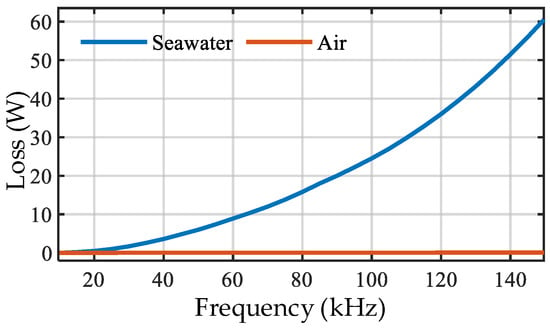
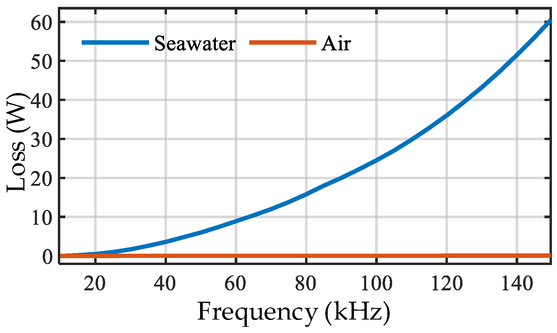
As shown in Figure 2, the equivalent eddy-current loss varies continuously with frequency; specifically, the eddy-current loss increases monotonically as the operating frequency increases. Moreover, as reported in [27], for an IPT system operating in an underwater environment, the eddy-current loss can be modeled by an equivalent resistance. The corresponding analytical expressions are given in (3) and (4).

$$R_{eddy1}={\displaystyle \frac{2k{\omega }^2{\left|\frac{\mu }{4\pi }{\displaystyle \sum _{i=1}^{N_i}\frac{d{r}_i\times {\widehat{R}}_i}{R_i^2}}\right|}^2\pi h{r}^4\sigma }{3}}$$

(3)

$$R_{eddy2}={\displaystyle \frac{2k{\omega }^2{\left|\frac{\mu }{4\pi }{\displaystyle \sum _{j=1}^{N_j}\frac{d{r}_j\times {\widehat{R}}_j}{R_j^2}}\right|}^2\pi h{r}^4\sigma }{3}}$$

(4)

where k is a correction factor, ω is the operating angular frequency, μ is the magnetic permeability, h is the separation distance between the plates, and σ is the electrical conductivity. As observed in (3) and (4), the equivalent resistance associated with eddy-current loss increases markedly with increasing frequency. Furthermore, from (1) and (2), it can be seen that once the geometric dimensions, materials, and other coil characteristics of the transmitting and receiving coils are fixed, R_eddy1 and R_eddy2 are proportional to ω². Therefore, (5) can be obtained.

$$\{\begin{array}{l}{R}_{eddy1\_f1}={\displaystyle \frac{{\omega }_1^2}{{\omega }_2^2}}\times R_{eddy1\_f2}\\ R_{eddy2\_f1}={\displaystyle \frac{{\omega }_1^2}{{\omega }_2^2}}\times R_{eddy2\_f2}\end{array}$$

(5)

Figure 2. Variation of system loss with frequency under different media conditions.

2.2. DLCC Equivalent Circuit and Input Impedance Derivation

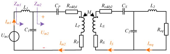
Based on the analysis in Section 2.1, a DLCC system is adopted, and the resulting equivalent circuit topology is further derived, as shown in Figure 3.

Figure 3. Equivalent circuit diagram of the underwater DLCC-IPT system.

L₁, C₁, and C_P are compensation components on primary side. L₂, C₂, and C_S are compensation components on the secondary side. Figure 3 shows the equivalent circuit of the DLCC-IPT system. According to Kirchhoff’s voltage law, the circuit equations for the primary and secondary coils of the equivalent model in Figure 3 can be written, yielding the relationship given in (6) and (7).

$$\{\begin{array}{l}\left(j\omega L_1+{\displaystyle \frac{1}{j\omega C_1}}\right)I_{in1}-{\displaystyle \frac{I_{in2}}{j\omega C_1}}=U_{in1}\\ \left({\displaystyle \frac{1}{j\omega C_1}}+{\displaystyle \frac{1}{j\omega C_P}}+R_P+R_{eddy 1}+j\omega L_P\right)I_{in2}-{\displaystyle \frac{1}{j\omega C_1}}{I}_{in1}=j\omega M{I}_S\\ \left({\displaystyle \frac{1}{j\omega C_2}}+{\displaystyle \frac{1}{j\omega C_S}}+R_S+R_{eddy 2}+j\omega L_S\right)I_S-{\displaystyle \frac{I_{req}}{j\omega C_2}}=j\omega M{I}_P\\ \left(j\omega L_2+R_{eq}+{\displaystyle \frac{1}{j\omega C_2}}\right)I_{req}-{\displaystyle \frac{I_S}{j\omega C_2}}=0\end{array}$$

(6)

$$\omega ={\displaystyle \frac{1}{\sqrt{L_1{C}_1}}}={\displaystyle \frac{1}{\sqrt{L_2{C}_2}}}={\displaystyle \frac{1}{\sqrt{\left(L_P-L_1\right)C_P}}}={\displaystyle \frac{1}{\sqrt{\left(L_S-L_2\right)C_S}}}$$

(7)

Therefore, by jointly solving the circuit equations given in (6) and (7), the theoretical expression for the system impedance can be derived. In particular, Z_{in1_rms_fx} and Z_{in2_rms_fx} are given by (9) and (10), respectively.

$$Z_{r\_rms\_fx}={\displaystyle \frac{{\omega }^2{M}^2}{j\omega L_S+1/j\omega C_S+R_{eddy2\_fx}+R_S+\left(j\omega L_2+R_{\mathrm{eq}}\right)/\left(1-{\omega }^2{C}_2{L}_2+j\omega C_2{R}_{\mathrm{eq}}\right)}}$$

(8)

$$Z_{in2\_rms\_fx}=Z_{r\_rms\_fx}+j\omega L_P+R_P+R_{eddy1\_fx}+{\displaystyle \frac{1}{j\omega C_P}}(fx=f1, f2)$$

(9)

$$Z_{in1\_rms\_fx}=j\omega L_1+{\displaystyle \frac{1}{j\omega C_1+1/Z_{in2\_rms\_fx}}}(fx=f1, f2)$$

(10)

The circuit parameters L₁, L_P, L_S, L₂, C₁, C_P, C_S, C₂, R_S, and R_P can be directly measured using an impedance analyzer. However, under underwater operating conditions, the M, R_{eddy1_fx}, R_{eddy2_fx}, and R_eq vary dynamically and therefore cannot be measured directly. The parameter vector to be identified is given in (11), while the measurement vector, which consists of the input impedance magnitudes of the two ports at different frequencies, is defined in (12). Here, Z_{r_rms_f1}, R_{eddy1_f1}, R_{eddy2_f1}, Z_{in1_rms_f1}, Z_{in2_rms_f1}, Z_{r_rms_f2}, R_{eddy1_f2}, R_{eddy2s_f2}, Z_{in1_rms_f2}, and Z_{in2_rms_f2} represent the true values of the measured impedances of Z_r, R_{eddy1_fx}, R_{eddy2_fx}, Z_in1, and Z_in2 at frequencies f₁ and f₂, respectively. For convenience in solving the identification problem, the equivalent eddy-current loss resistances at frequency f₂ are expressed in terms of those at frequency f₁. That is, at f₂, substituting (5) into (8)–(10) yields (8)–(13).

$$Z_{r\_rms\_f2}={\displaystyle \frac{{\omega }^2{M}^2}{j\omega L_S+1/j\omega C_S+{\left(f_2/f_1\right)}^2{R}_{eddy2\_f1}+R_S+\left(j\omega L_2+R_{\mathrm{eq}}\right)/\left(1-{\omega }^2{C}_2{L}_2+j\omega C_2{R}_{\mathrm{eq}}\right)}}$$

(11)

$$Z_{in2\_rms\_f2}=Z_{r\_rms\_f2}+j\omega L_P+R_P+{\left(f_2/f_1\right)}^2{R}_{eddy1\_f1}+{\displaystyle \frac{1}{j\omega C_P}}$$

(12)

$$Z_{in1\_rms\_f2}=j\omega L_1+{\displaystyle \frac{1}{j\omega C_1+1/Z_{in2\_rms\_f2}}}$$

(13)

Based on the above derivation of the circuit equations for the LCC-LCC IPT system, (14) can be obtained.

$$\{\begin{array}{l}\left|Z_{in1\_rms\_f1}\right|=\left|j\omega L_1+{\displaystyle \frac{1}{j\omega C_1+1/Z_{in2\_rms\_f1}}}\right|\\ \left|Z_{in1\_\mathrm{mea}\_f1}\right|=U_{in1\_\mathrm{mea}\_f1}/I_{in1\_\mathrm{mea}\_f1}\\ \left|Z_{in1\_rms\_f2}\right|=\left|j\omega L_1+{\displaystyle \frac{1}{j\omega C_1+1/Z_{in2\_rms\_f2}}}\right|\\ \left|Z_{in1\_\mathrm{mea}\_f2}\right|=U_{in1\_\mathrm{mea}\_f2}/I_{in1\_\mathrm{mea}\_f2}\\ \left|Z_{in2\_rms\_f1}\right|=\left|Z_{r\_rms\_f1}+j\omega L_P+R_P+R_{eddy1\_f1}+{\displaystyle \frac{1}{j\omega C_P}}\right|\\ \left|Z_{in2\_\mathrm{mea}\_f1}\right|=U_{in2\_\mathrm{mea}\_f1}/I_{in2\_\mathrm{mea}\_f1}\\ \left|Z_{in2\_rms\_f2}\right|=\left|Z_{r\_rms\_f2}+j\omega L_P+R_P+{\left(f_2/f_1\right)}^2{R}_{eddy1\_f1}+{\displaystyle \frac{1}{j\omega C_P}}\right|\\ \left|Z_{in2\_\mathrm{mea}\_f2}\right|=U_{in2\_\mathrm{mea}\_f2}/I_{in2\_\mathrm{mea}\_f2}\end{array}$$

(14)

where, U_{in1_mea_f1}, I_{in1_mea_f1}, U_{in2_mea_f1}, and I_{in2_mea_f1} denote the measured true values of U_in1, I_in1, U_in2, and I_in2, respectively, at the frequency f₁. Similarly, U_{in1_mea_f2}, I_{in1_mea_f2}, U_{in2_mea_f2}, I_{in2_mea_f2} denote the measured true values of U_in1, I_in1, U_in2, and I_in2, respectively, at the frequency f₂. Therefore, (15) can be finally established.

$$\{\begin{array}{l}\left|Z_{in1\_rms\_f1}\right|=\left|Z_{in1\_\mathrm{mea}\_f1}\right|\\ \left|Z_{in1\_rms\_f2}\right|=\left|Z_{in1\_\mathrm{mea}\_f2}\right|\\ \left|Z_{in2\_rms\_f1}\right|=\left|Z_{in2\_\mathrm{mea}\_f1}\right|\\ \left|Z_{in2\_rms\_f2}\right|=\left|Z_{in2\_\mathrm{mea}\_f2}\right|\end{array}$$

(15)

According to (15), the R_{eddy1_f1}, R_{eddy2_f1}, M, and the load R_eq, can be incorporated into the impedances |Z_{in1_rms_fx}| and |Z_{in2_rms_fx}|. Here, impedance magnitude is adopted, because it is more robust than the impedance phase in practical measurements. Since a single impedance magnitude may be insufficient to constrain multiple unknown parameters, two impedance magnitude measurements are jointly used to reduce ambiguity and improve identification accuracy. Accordingly, (16) can be obtained as follows:

$$\{\begin{array}{l}\left|Z_{in1\_rms\_f1}\right|=h_{in1\_rms\_f1}(R_{eddy1\_f1},R_{eddy2\_f1},M,R_{eq})\\ \left|Z_{in1\_rms\_f2}\right|=h_{in1\_rms\_f2}(R_{eddy1\_f1},R_{eddy2\_f1},M,R_{eq})\\ \left|Z_{in2\_rms\_f1}\right|=h_{in2\_rms\_f1}(R_{eddy1\_f1},R_{eddy2\_f1},M,R_{eq})\\ \left|Z_{in2\_rms\_f2}\right|=h_{in2\_rms\_f2}(R_{eddy1\_f1},R_{eddy2\_f1},M,R_{eq})\end{array}$$

(16)

By performing a first-order Taylor expansion of (16), the following expression is obtained:

$$\begin{array}{cc}\hfill \left|Z_{in1\_rms\_fx}\right|-\left|Z_{in1\_rms\_fx\_0}\right|& =\left(R_{eddy1\_f1}-R_{eddy1\_f1\_0}\right){\displaystyle \frac{\partial \left|Z_{in1\_rms\_fx}\right|}{\partial R_{eddy1\_f1}}}+\left(R_{eddy2\_f1}-R_{eddy2\_f1\_0}\right){\displaystyle \frac{\partial \left|Z_{in1\_rms\_fx}\right|}{\partial R_{eddy2\_f1}}}\hfill \\ & +\left(M-M_0\right){\displaystyle \frac{\partial \left|Z_{in1\_rms\_fx}\right|}{\partial M}}+\left(R_{eq}-R_{eq\_0}\right){\displaystyle \frac{\partial \left|Z_{in1\_rms\_fx}\right|}{\partial R_{eq}}}+R_{1,2}\hfill \end{array}$$

(17)

$$\begin{array}{cc}\hfill \left|Z_{in2\_rms\_fx}\right|-\left|Z_{in2\_rms\_fx\_0}\right|& =\left(R_{eddy1\_f1}-R_{eddy1\_f1\_0}\right){\displaystyle \frac{\partial \left|Z_{in2\_rms\_fx}\right|}{\partial R_{eddy1\_f1}}}+\left(R_{eddy2\_f1}-R_{eddy2\_f1\_0}\right){\displaystyle \frac{\partial \left|Z_{in2\_rms\_fx}\right|}{\partial R_{eddy2\_f1}}}\hfill \\ & +\left(M-M_0\right){\displaystyle \frac{\partial \left|Z_{in2\_rms\_fx}\right|}{\partial M}}+\left(R_{eq}-R_{eq\_0}\right){\displaystyle \frac{\partial \left|Z_{in2\_rms\_fx}\right|}{\partial R_{eq}}}+R_{3,4}\hfill \end{array}$$

(18)

In (17) and (18), |Z_{in1_rms_fx_0}| and |Z_{in2_rms_fx_0}| denote the values of the corresponding functions at the point (R_{eddy1_f1_0}, R_{eddy2_f1_0}, M_{_0}, R_{eq_0}), and R_n is the higher-order remainder term and is neglected in the subsequent analysis. At multiple frequencies, a set of equations can be formed based on (16), which can be represented in matrix form as Y = JX, where:

$$Y=\left[\begin{array}{c}\left|Z_{in1\_rms\_f1}\right|-\left|Z_{in1\_rms\_f1\_0}\right|\\ \left|Z_{in1\_rms\_f2}\right|-\left|Z_{in1\_rms\_f2\_0}\right|\\ \left|Z_{in2\_rms\_f1}\right|-\left|Z_{in2\_rms\_f1\_0}\right|\\ \left|Z_{in2\_rms\_f2}\right|-\left|Z_{in2\_rms\_f2\_0}\right|\end{array}\right]$$

(19)

$$J=\left[\begin{array}{cccc}{\displaystyle \frac{\partial \left|Z_{in1\_rms\_f1}\right|}{\partial R_{eddy1\_f1}}}& {\displaystyle \frac{\partial \left|Z_{in1\_rms\_f1}\right|}{\partial R_{eddy2\_f1}}}& {\displaystyle \frac{\partial \left|Z_{in1\_rms\_f1}\right|}{\partial M}}& {\displaystyle \frac{\partial \left|Z_{in1\_rms\_f1}\right|}{\partial R_{eq}}}\\ {\displaystyle \frac{\partial \left|Z_{in1\_rms\_f2}\right|}{\partial R_{eddy1\_f1}}}& {\displaystyle \frac{\partial \left|Z_{in1\_rms\_f2}\right|}{\partial R_{eddy2\_f1}}}& {\displaystyle \frac{\partial \left|Z_{in1\_rms\_f2}\right|}{\partial M}}& {\displaystyle \frac{\partial \left|Z_{in1\_rms\_f2}\right|}{\partial R_{eq}}}\\ {\displaystyle \frac{\partial \left|Z_{in2\_rms\_f1}\right|}{\partial R_{eddy1\_f1}}}& {\displaystyle \frac{\partial \left|Z_{in2\_rms\_f1}\right|}{\partial R_{eddy2\_f1}}}& {\displaystyle \frac{\partial \left|Z_{in2\_rms\_f1}\right|}{\partial M}}& {\displaystyle \frac{\partial \left|Z_{in2\_rms\_f1}\right|}{\partial R_{eq}}}\\ {\displaystyle \frac{\partial \left|Z_{in2\_rms\_f2}\right|}{\partial R_{eddy1\_f1}}}& {\displaystyle \frac{\partial \left|Z_{in2\_rms\_f2}\right|}{\partial R_{eddy2\_f1}}}& {\displaystyle \frac{\partial \left|Z_{in2\_rms\_f2}\right|}{\partial M}}& {\displaystyle \frac{\partial \left|Z_{in2\_rms\_f2}\right|}{\partial R_{eq}}}\end{array}\right]$$

(20)

$$X={\left[\begin{array}{cccc}{R}_{eddy1\_f1}-R_{eddy1\_f1\_0}& R_{eddy2\_f1}-R_{eddy2\_f1\_0}& M-M_0& R_{eq}-R_{eq\_0}\end{array}\right]}^T$$

(21)

It follows from (20) that, with a sufficiently rich selection of operating frequencies and the adoption of dual impedance-magnitude constraints, there exist cases in which the Jacobian matrix J has rank 4.

$$f\left(x\right)={\displaystyle \sum _{\mathrm{x}=1}^2\left|\left(\left|Z_{in1\_rms\_fx}\right|-\left|Z_{in1\_mea\_fx}\right|\right)+\left(\left|Z_{in2\_rms\_fx}\right|-\left|Z_{in2\_mea\_fx}\right|\right)\right|}$$

(22)

3. Proposed Multi-Parameter Identification Method

Based on the system model established in the preceding sections, to address the identification of the four unknown parameters R_eq, M, R_{eddy1_f1}, and R_{eddy2_f1}, this section proposes a hybrid particle swarm optimization algorithm, developed by improving and integrating the conventional genetic algorithm and particle swarm optimization.

3.1. Genetic Algorithm (GA) and Particle Swarm Optimization (PSO)

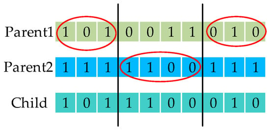
GA is an optimization method inspired by natural selection and genetic mechanisms, and it is suitable for complex optimization problems such as non-convex and non-smooth ones. The algorithm takes the initial solution of encoding a population composed of individuals, and each individual corresponds to a chromosome. The initial population is generated by random sampling. Optimal individuals are selected based on fitness, and new populations are generated through crossover and variation, as shown in Figure 4.

Figure 4. Crossover operation diagram.

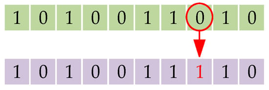
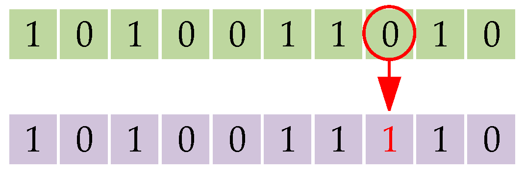
The genes of the chromosome are randomly modified, as shown in Figure 5.

Figure 5. Mutation operation diagram.

Although GA maintains population diversity, it may generate low quality offspring, thereby leading to performance degradation.

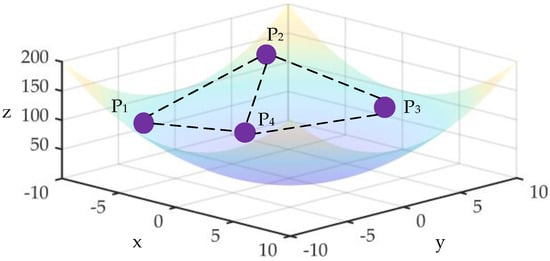
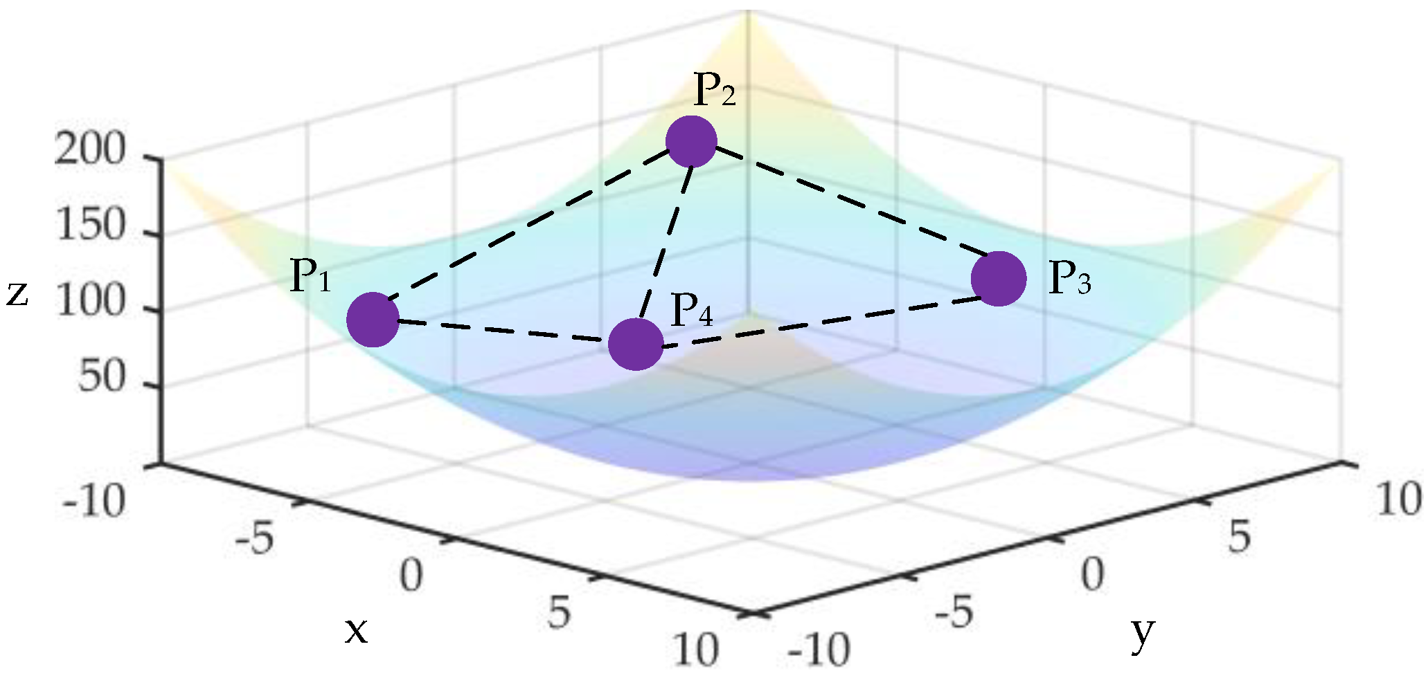
PSO updates the velocity and position of each particle according to the individual best and global best information, thereby balancing global exploration and local exploitation and gradually approaching better solutions, as shown in Figure 6.

Figure 6. PSO position-velocity update diagram.

PSO often suffers from premature convergence and reduced population diversity when dealing with complex objective functions or high-dimensional problems, resulting in unstable convergence performance.

3.2. Hybrid Particle Swarm Optimization (HPSO)

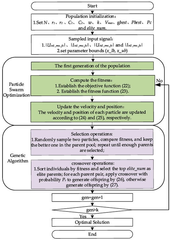
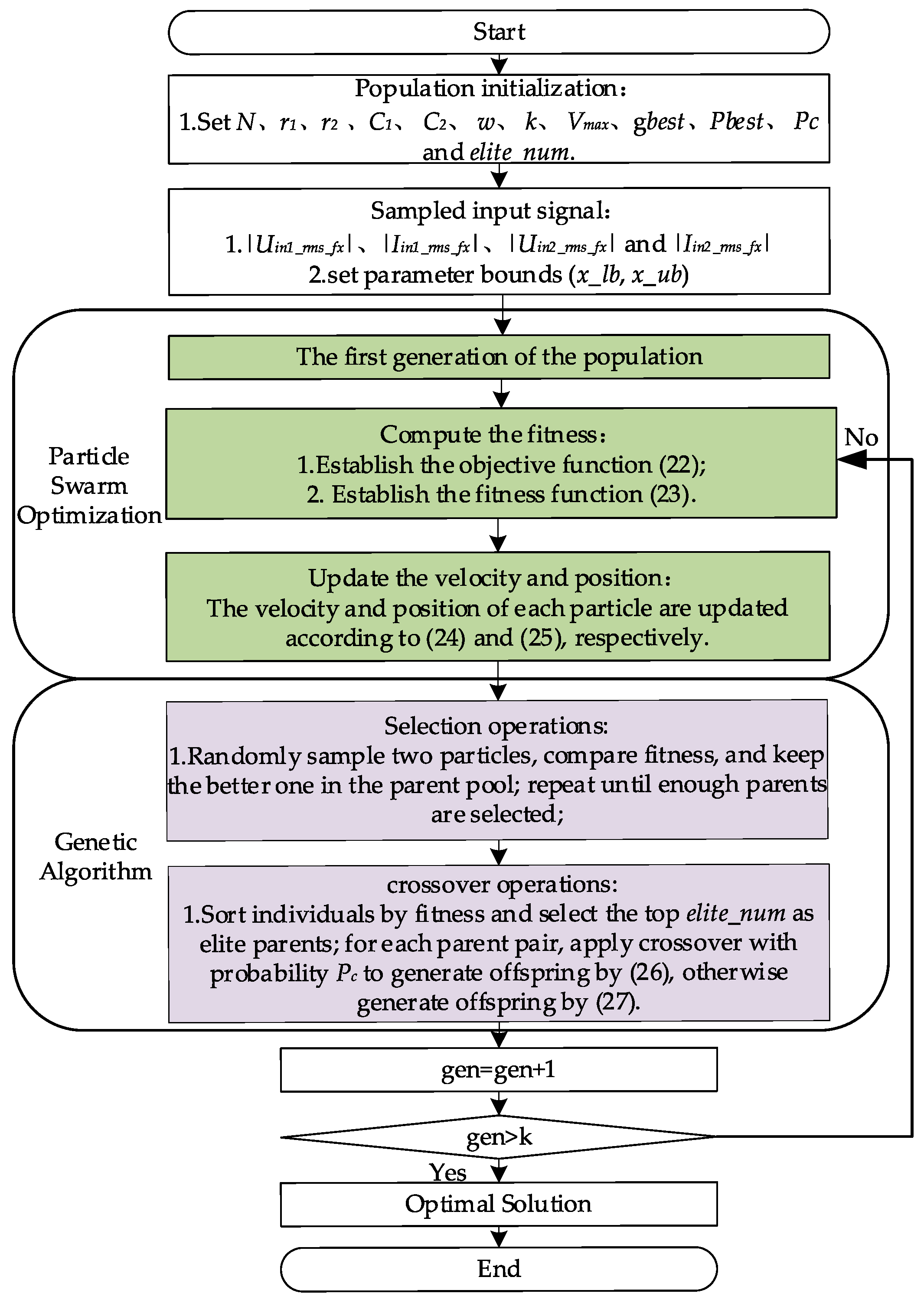
Although GA exhibits strong global exploration capability, and PSO features fast convergence, each algorithm still has certain limitations when applied to multi-parameter identification problems. GA may suffer from slow convergence in the later stage of evolution, whereas PSO is prone to premature convergence and local optima in complex multimodal search spaces. To take advantage of the complementary strengths of both methods, this study adopts a hybrid particle swarm optimization algorithm (HPSO), in which genetic operators are incorporated into the particle swarm iteration process. By enhancing population diversity and global exploration capability while maintaining the fast convergence characteristic of PSO, HPSO provides a more effective solution to the parameter identification problem addressed in this paper. The specific implementation steps are as follows:

Step1: Initialize the required parameters, set n as the population size; r₁ and r₂ are the random numbers in the [0, 1] interval, G₁ and G₂ correspond to acceleration coefficients, w_i corresponds to the inertia weight, V_max is the maximum particle velocity, P_C is the crossover probability, P_best is the individual optimal position, g_best is the global optimal position, α is the coefficient of variation, and elite_num is the number of elite particles retained in the selection process.

Step2: Construct the objective function and compute the fitness value. To more intuitively characterize the degree of matching between the theoretical and actual impedance values, the objective function in (22) is transformed into the fitness function in (23), whose value approaches 1.

$$e={\displaystyle \frac{1}{1+f\left(x\right)}}$$

(23)

Step3: Update the velocity and position. Ref. (24) represents the velocity update of the i-th particle at the d-th iteration, $v_i^d$ and $v_i^{d+1}$ denote the corresponding particle velocities, respectively. Ref. (25) indicates that the new position is obtained by adding the velocity vector to the current position; $X_i^d$ and $X_i^{d+1}$ denote the corresponding particle positions, respectively.

$$v_i^{d+1}=\omega \times v_i^d+G_1\times r_1\times (pbest-x_i^d)+G_2\times r_2\times (gbest-x_i^d)$$

(24)

$$X_i^{d+1}=X_i^d+V_i^{d+1}$$

(25)

Step4: Perform elite selection and crossover operations. With a probability of P_C, the offspring are mutated as shown in (26); otherwise, they remain unchanged as shown in (27). $X_{i_{2k}}^{\prime }$ and $X_{i_{2k-1}}^{\prime }$ both denote the parent individuals, while $X_{i_{2k-1}}$ and $X_{i_{2k}}$ both denote the offspring particles generated through crossover.

$$\{\begin{array}{l}{X}_{i_{2k-1}}^{\prime }=\alpha \times X_{i_{2k-1}}^{\prime }+(1-\alpha )\times X_{i_{2k}}\hfill \\ X_{i_{2k}}^{\prime }=(1-\alpha )\times X_{i_{2k-1}}^{\prime }+\alpha \times X_{i_{2k}}\hfill \end{array}$$

(26)

$$X_{i_{2k-1}}^{\prime }=X_{i_{2k-1}},\hspace{1em}{X}_{i_{2k}}^{\prime }=X_{i_{2k}}$$

(27)

Whenever a new set of valid inputs is provided, the hybrid particle swarm algorithm outputs the corresponding predicted value of the mapping relationship, ultimately yielding the identified results of the four parameters. Figure 7 shows the flowchart of the multi-parameter identification method.

Figure 7. Flowchart of the parameter identification algorithm based on hybrid particle swarm optimization.

3.3. Simulation Results

To verify the practical feasibility and identification performance of the proposed method, a DLCC simulation model was established based on the structure shown in Figure 3, and the parameters of each component are listed in Table 1.

Table 1. System parameters.

Parameter	Value	Parameter	Value
Uin (V)	100	f (kHz)	50~120
LP (μH)	144.3	LS (μH)	144.2
RP (Ω)	0.36	RS (Ω)	0.35
L1 (μH)	25.3	L2 (μH)	51.0
C1 (nF)	138.1	C2 (nF)	68.8
CP (nF)	28.8	CS (nF)	38.2
M (μH)	20~50	RL (Ω)	30~50
Reddy2, Reddy1 (Ω)	0.5~2	k	0.24

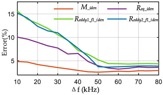
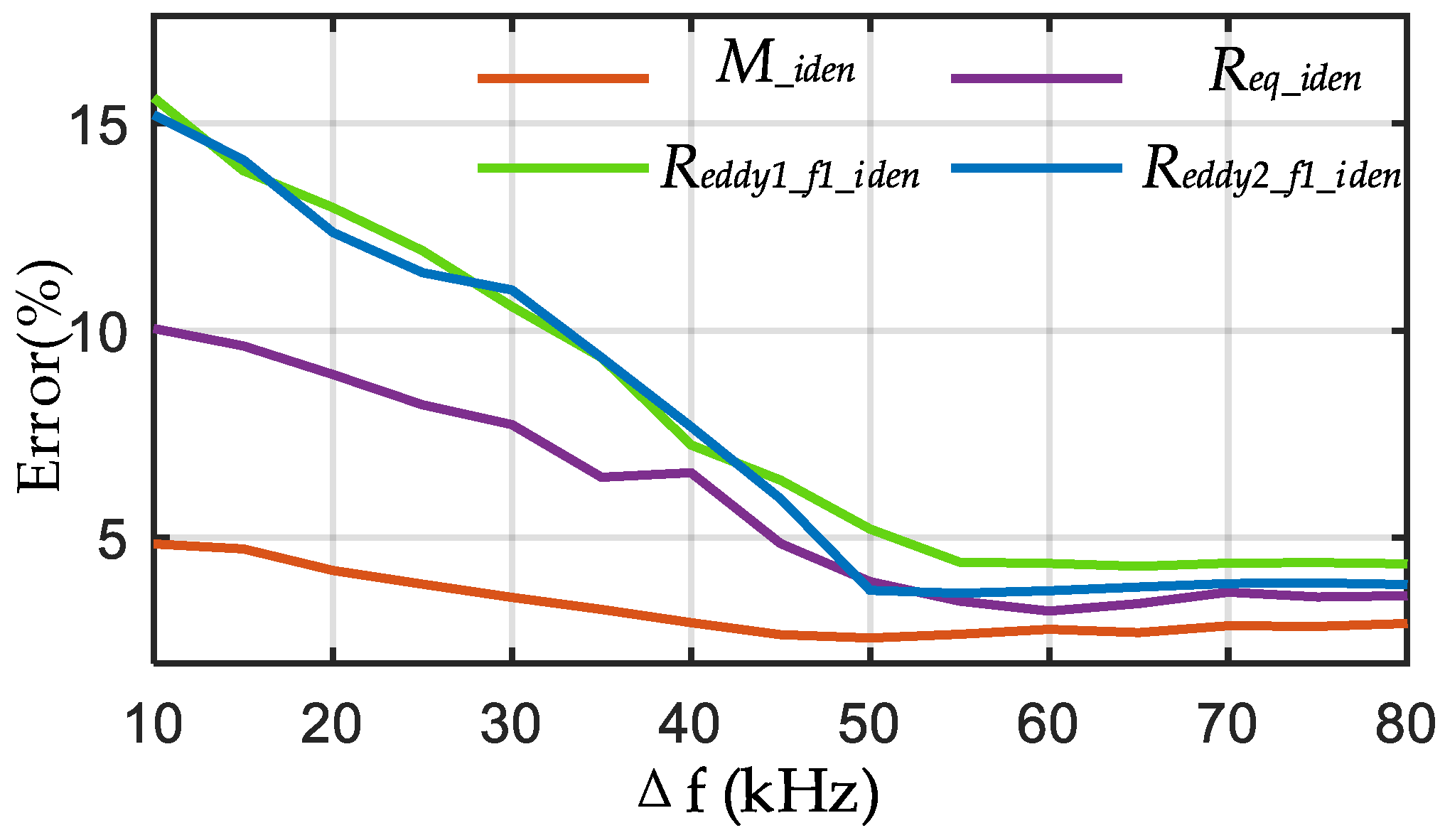
To identify the four unknown parameters, two frequency-switching operations are required. Therefore, the simulation experiments are conducted at two operating frequencies; after each change of the operating frequency, the RMS values of the relevant voltages and currents under that frequency condition are collected and recorded. The coil spacing is set to 10 cm, the conductivity is set to 8 S/m, and the load resistance is set to 45 Ω. Based on the parameters in Table 1, with 85 kHz as the center frequency, a frequency sweep is carried out to select the optimal two simulation frequencies. In Figure 8, the horizontal coordinate Δf represents the frequency offset from the center frequency of 85 kHz, meaning that the two operating frequencies are selected symmetrically as 85 − (Δf/2) and 85 + (Δf/2) kHz.

Figure 8. Relationship between the frequency offset Δf and the identification error.

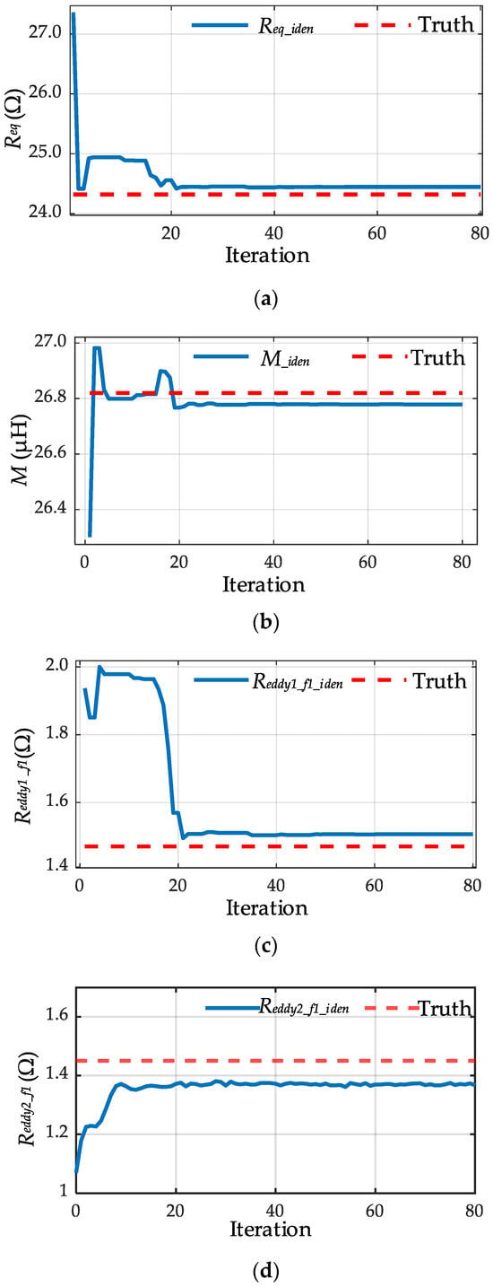
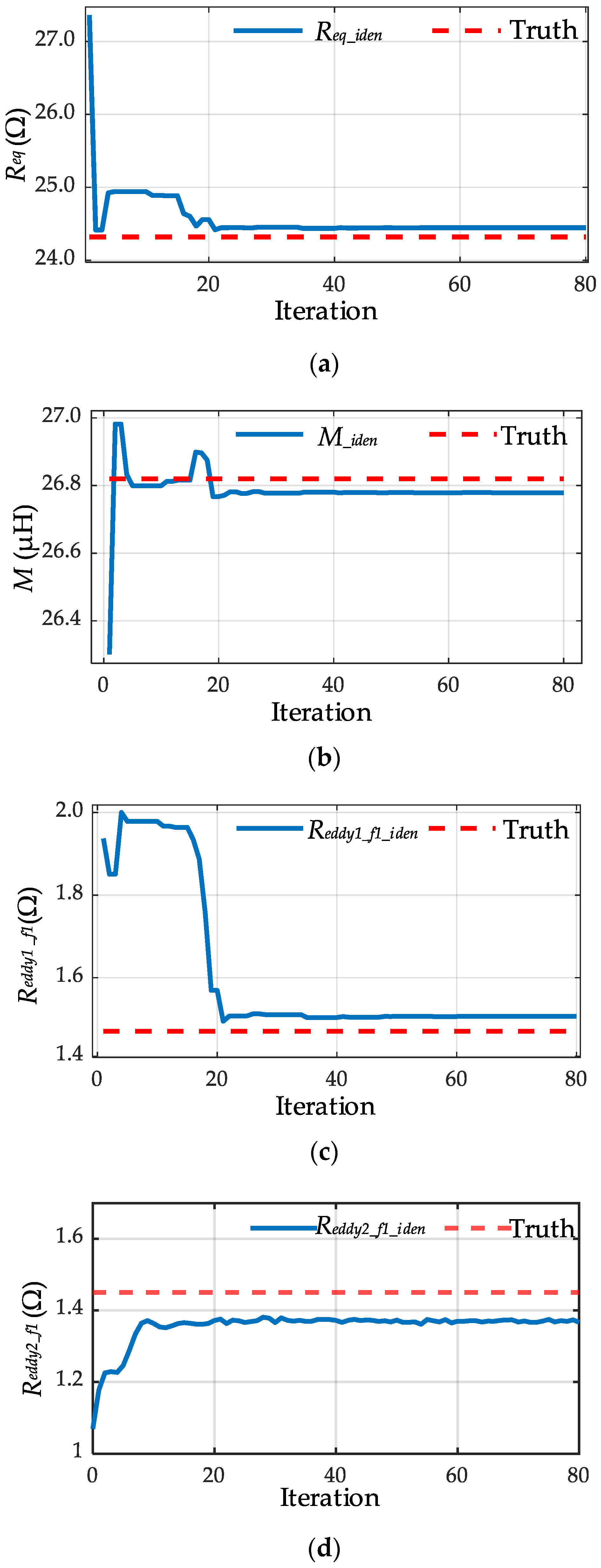
As shown in Figure 8, the identification error is related to the frequency separation between the two selected operating points. When the two frequencies are too close, the corresponding impedance magnitudes exhibit similar variations, resulting in weaker parameter sensitivity and slightly reduced identification accuracy. As the frequency offset increases, the identification error decreases and then gradually stabilizes. This indicates that a moderate frequency separation is sufficient to obtain reliable identification performance. Therefore, 50 kHz and 120 kHz are selected in this study as a practical choice. It should also be noted that the proposed method is not limited to this specific frequency pair; other frequency combinations can also be used, provided that sufficient parameter sensitivity is preserved and the adopted frequency-dependent model remains valid. Under this frequency configuration, the variations in the parameters to be identified with the number of iterations are shown in Figure 9.

Figure 9. Relationship between identified parameters and iteration count: (a) Relationship between R_eq and Iteration; (b) Relationship between M and Iteration; (c) Relationship between R_{eddy1_f1} and Iteration; (d) Relationship between R_{eddy2_f1} and Iteration.

As shown in Figure 9, the identification results become essentially stable after 20 iterations; therefore, 40 iterations are adopted in this study. To quantitatively evaluate the identification accuracy of the proposed method, the relative error is used as the evaluation metric to uniformly measure the identification results of the load resistance, mutual inductance, and the eddy-current loss equivalent resistance, as given in (28). Where R_{eq_iden}, M_iden, R_{eddy1_f1_iden}, and R_{eddy2_f1_iden} are the identified parameter values, and R_{eq_truth}, M_truth, R_{eddy1_f1_truth}, and R_{eddy2_f1_truth} are the true values.

$$error={\displaystyle \frac{\left|R_{eq\_iden}-R_{eq\_truth}\right|}{R_{eq\_truth}}}+{\displaystyle \frac{\left|M_{iden}-M_{truth}\right|}{M_{truth}}}+{\displaystyle \frac{\left|R_{eddy1\_f1\_iden}-R_{eddy1\_f1\_truth}\right|}{R_{eddy1\_f1\_truth}}}+{\displaystyle \frac{\left|R_{eddy2\_f1\_iden}-R_{eddy2\_f1\_truth}\right|}{R_{eddy2\_f1\_truth}}}$$

(28)

To verify the applicability and robustness of the algorithm under complex operating conditions, the system operating frequencies are set to 120 kHz and 50 kHz, and multiple typical scenarios are constructed for comparative experiments. Under different coil spacings and medium conductivities, the load resistance is varied to emulate power consumption changes of an AUV across different operating stages. By statistically analyzing and comparing the identification errors for each scenario, the effectiveness of the proposed method is further validated when the frequency-dependent characteristics of eddy-current losses are taken into account.

3.4. Analysis of Parameter Drift and Noise

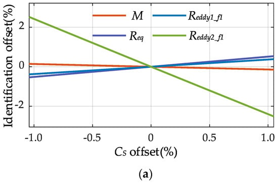
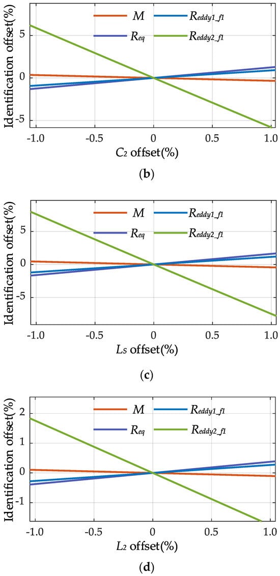
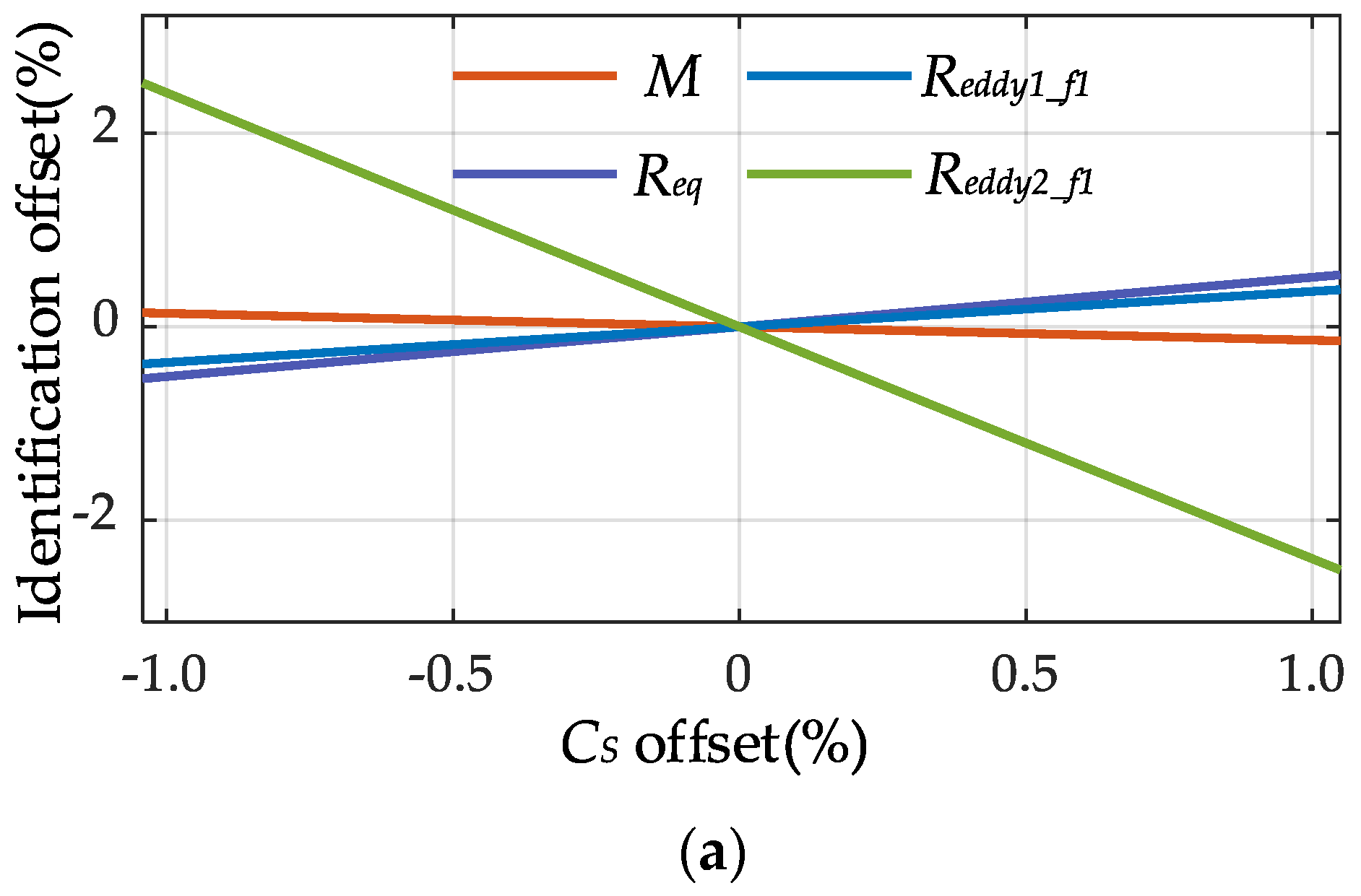
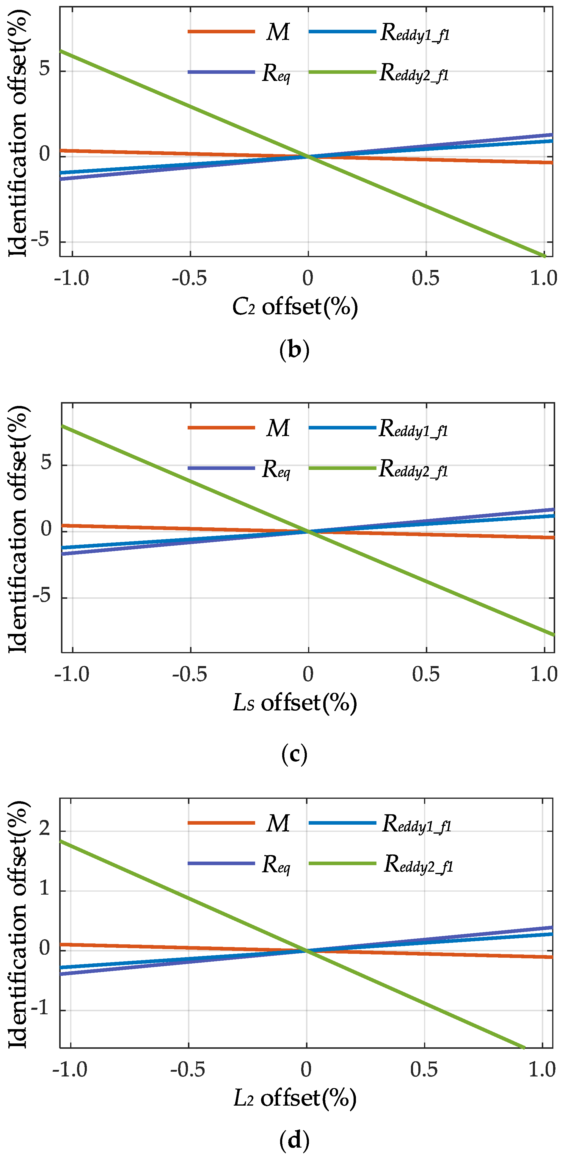
In practical underwater IPT systems, component drift caused by temperature variation, aging, manufacturing tolerance, and environmental disturbance is difficult to avoid. When drift occurs on the secondary side, direct measurement is often inconvenient, and the resulting parameter mismatch may affect the reflected impedance observed from the primary side, thereby influencing parameter identification. This subsection therefore analyzes the effect of secondary side parameter drift on the extracted results. The drift of the secondary compensation parameters C_S, C₂, L_S, and L₂ is considered, and since the identification of M, R_eq, R_eddy1, and R_eddy2 mainly depends on the reflected impedance, the corresponding extraction relationships are established using the reflected-impedance model. By perturbing C_S, C₂, L_S, and L₂ around their nominal values while keeping the other parameters unchanged, the resulting extraction errors of M, R_eq, R_{eddy1_f1}, and R_{eddy2_f1} can be obtained, as shown in Figure 10.

Figure 10. Influence of secondary side parameter drift on the extracted values of M, R_eq, R_{eddy1_f1}, and R_{eddy2_f1}: (a) Identification errors of M, R_eq, R_{eddy1_f1}, and R_{eddy2_f1} under C_S drift; (b) Identification errors of M, R_eq, R_{eddy1_f1}, and R_{eddy2_f1} under C₂ drift; (c) Identification errors of M, R_eq, R_{eddy1_f1}, and R_{eddy2_f1} under L_S drift; (d) Identification errors of M, R_eq, R_{eddy1_f1}, and R_{eddy2_f1} under L₂ drift.

As shown in Figure 10a–d, drifts in the secondary side compensation parameters lead to deviations in the extracted values of M, R_eq, R_{eddy1_f1}, and R_{eddy2_f1}, with different sensitivities. Overall, the proposed method remains relatively stable under moderate parameter drift, whereas larger compensation mismatch may reduce the extraction accuracy.

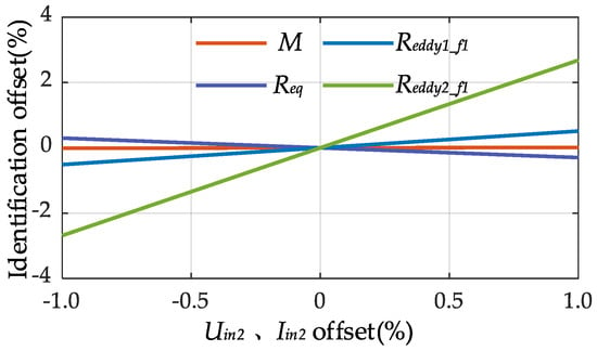
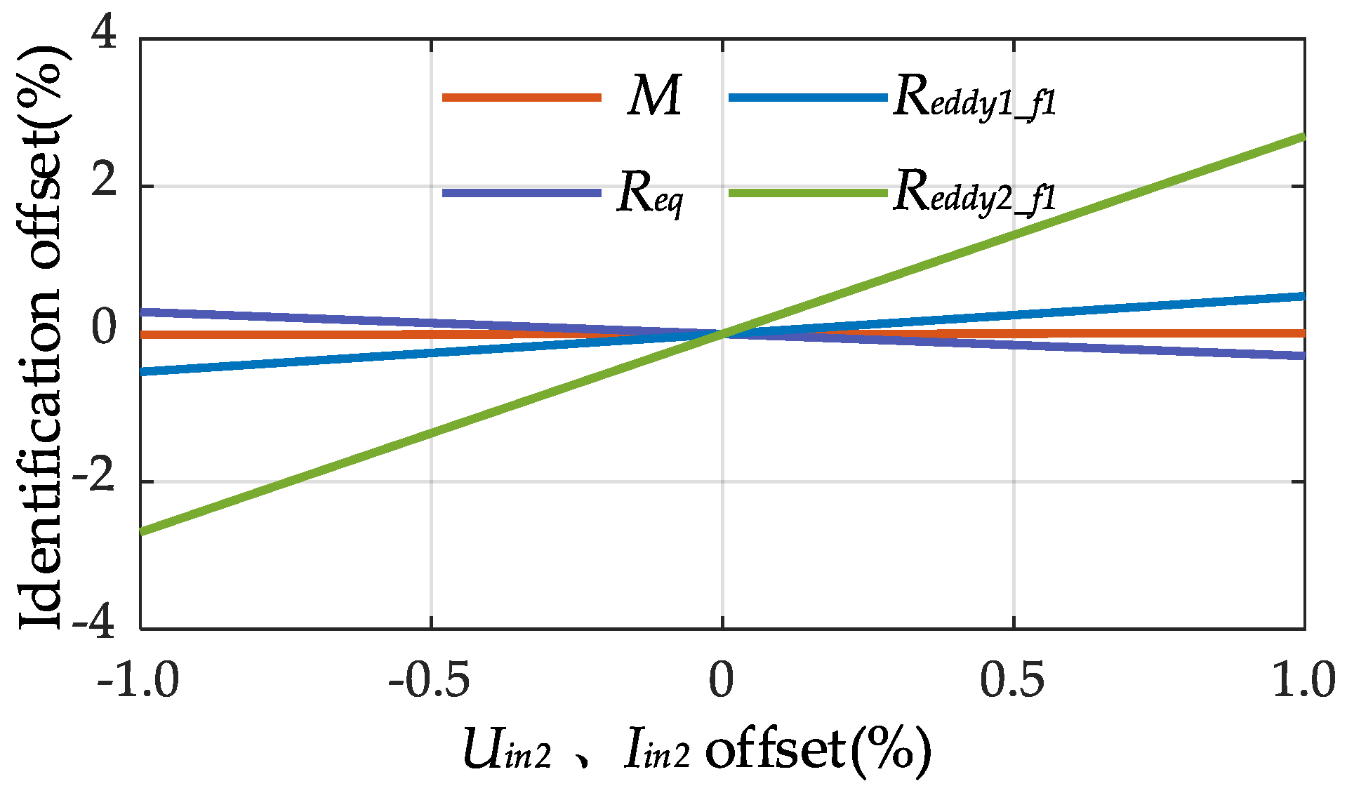
In practical underwater IPT systems, measurement noise in voltage and current signals is unavoidable and may propagate into parameter identification results through the calculated input impedance. To analyze this effect, noisy measurement models are established and the corresponding impedance perturbation is derived. Then, based on the impedance expression at frequency f₁, the unknown parameters R_{eddy1_f1}, R_{eddy2_f1}, R_eq, and M are decoupled and represented by explicit extraction functions, allowing the influence of impedance deviation on the identified parameters to be quantitatively evaluated. Furthermore, a ± 1% perturbation is introduced into the measured voltage and current signals, and the resulting identification error curves are presented in Figure 11.

Figure 11. Influence of measurement noise on the identified parameters.

It can be observed that the identified values of R_{eddy1_f1}, R_{eddy2_f1}, R_eq, and M show only slight fluctuations in the presence of measurement noise, while the overall relative error remains relatively small. This suggests that the proposed method is feasible under the multi-frequency impedance framework and shows acceptable tolerance to practical measurement disturbances, which may support its application in underwater IPT systems.

4. Experimental Verification

4.1. Experimental Platform and System Parameters

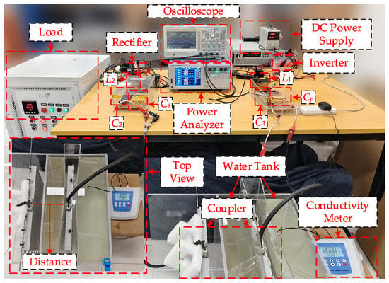
To verify the feasibility and accuracy of the proposed parameter identification method, an underwater IPT system based on a DLCC compensation topology was constructed, as shown in Figure 12. The experimental platform consists of a DC power supply (IT6018D−1500−40), an inverter and a rectifier implemented based on the DSP unit TMS320F28335 primary side and secondary side compensation networks (KG−IR−COM), a coupler, and a load (SX−30KWD800−W7A). An oscilloscope (ZDS3024Plus) and a power analyzer (WT1804E) were employed to measure the input and output electrical quantities. In addition, a water tank and a conductivity meter (DDS−11A) were used to provide a controllable and measurable medium environment, thereby enabling repeatable configurations of three categories of parameters: transfer distance, medium conductivity, and load.

Figure 12. Experimental platform.

Based on the experimental platform, this study designed eight representative operating conditions (in Table 2) to verify the parameter identification accuracy of the proposed method under multi-operating condition variation scenarios.

Table 2. Experimental conditions.

Conditions	Distance (cm)	Conductivity (S/m)	Load Resistance (Ω)	M (μH)	Reddy1 (Ω)	Reddy2 (Ω)	Req (Ω)
P1	15	6	30	26.82	1.47	1.45	24.32
P2	20	6	30	16.38	1.47	1.45	24.32
P3	15	3	30	26.82	0.73	0.70	24.32
P4	20	3	30	16.38	0.73	0.70	24.32
P5	15	6	45	26.82	1.47	1.45	36.48
P6	20	6	45	16.38	1.47	1.45	36.48
P7	15	3	45	26.82	0.73	0.70	36.48
P8	20	3	45	16.38	0.73	0.70	36.48

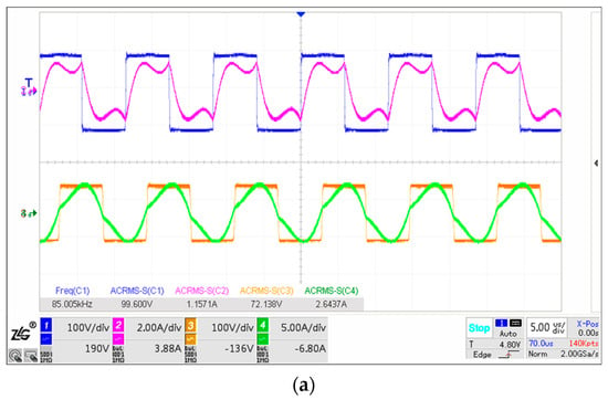
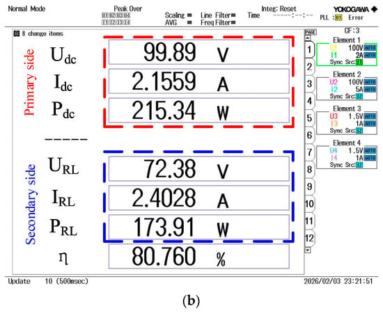
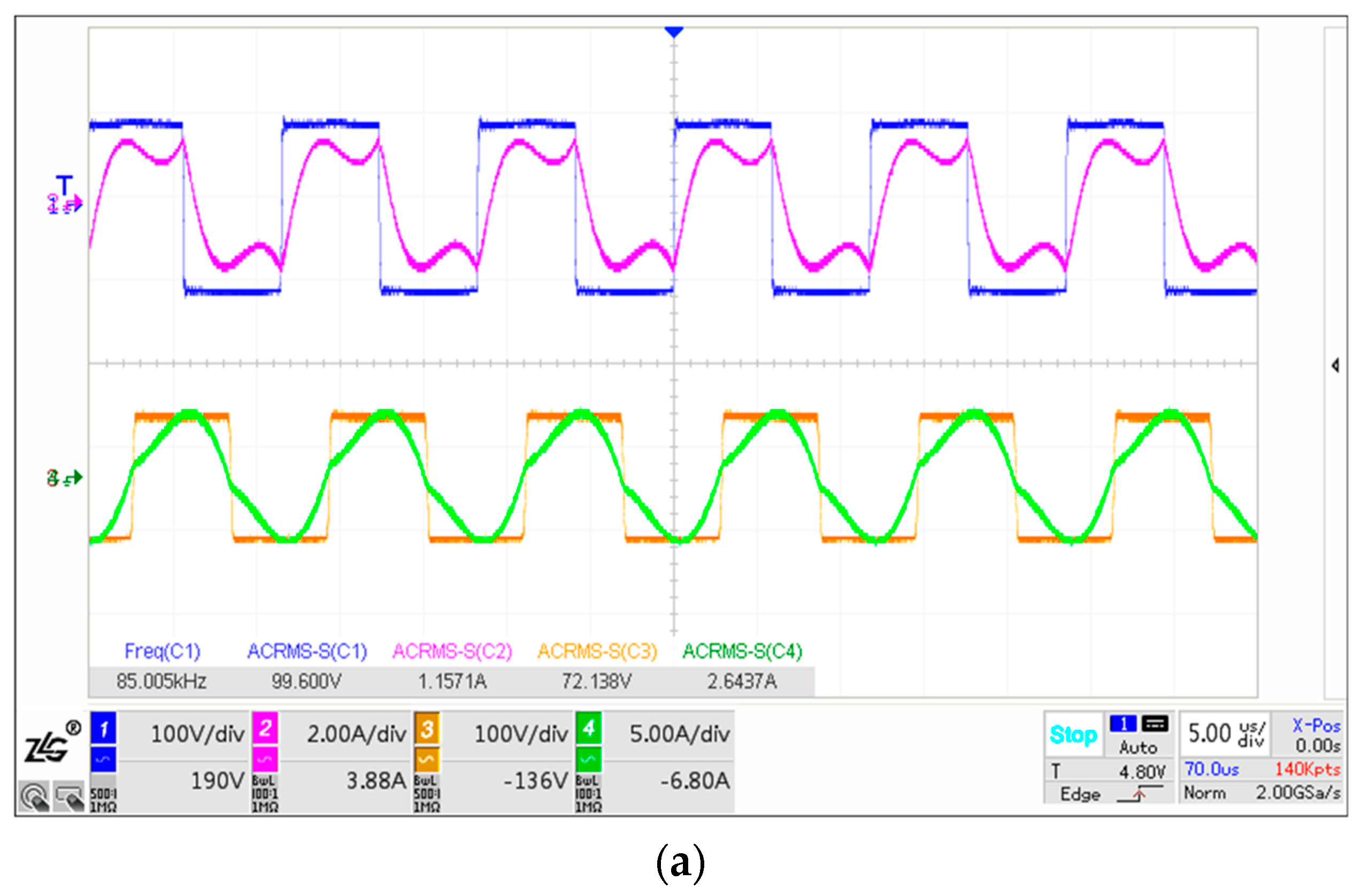
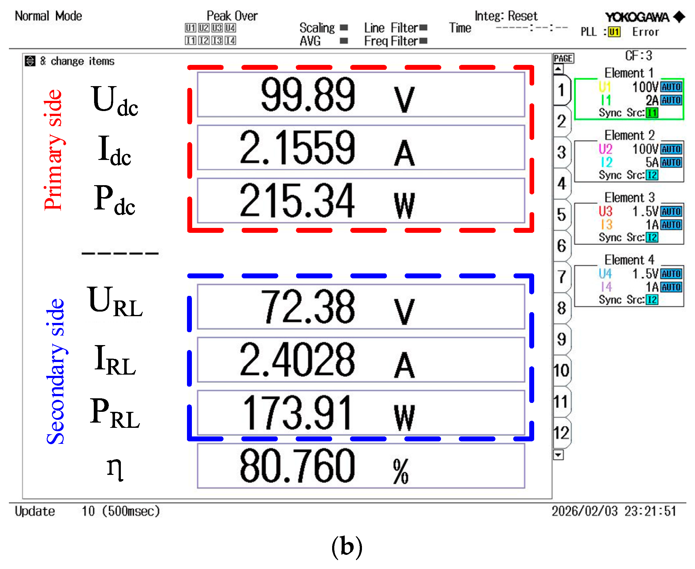
To verify the operational reliability of the system at 85 kHz under operating condition 1, experimental tests were conducted to measure the inverter-side voltage, current, and input power, as well as the rectified load-side voltage, current, and output power. The corresponding steady state waveforms and power measurement results are also reported.

As shown in Figure 13, under operating condition P1 at 85 kHz, the system achieves stable energy transfer and power conversion, with an overall efficiency of approximately 80.76%. This indicates that the operating point is highly feasible and stable, and can serve as the baseline condition for subsequent method validation. Based on the experimental feasibility under this baseline condition, this study further extends the validation to multi-condition scenarios and conducts two sets of comparative experiments. In the first set, the water conductivity is kept constant, and the receiving coil to AUV housing spacing and the internal load resistance of the AUV are varied to evaluate parameter identification accuracy. In the second set, the water conductivity is further varied on this basis to analyze the identification performance under different environmental parameters. Experiments are configured group by group according to Table 2, and parameter identification and error statistical analyses are performed to comprehensively assess the identification accuracy, applicability, and stability under different operating conditions.

Figure 13. System operating state diagram: (a) Primary and secondary side voltage and current waveforms; (b) Measured input and output parameters and transfer efficiency.

4.2. Mutual Inductance and Load Variation Identification Experiments

To verify the applicability of the proposed method under conditions where the coupling state varies simultaneously with load changes, this section selects four operating points (P1, P2, P5, and P6) in Table 2 to conduct identification experiments. Among them, P1 and P2 correspond to different coil spacings, with the load maintained at 30 Ω; P5 and P6 keep the same spacing settings but adjust the load to 45 Ω. During the experiments, the system operates at two working frequencies (120 kHz and 50 kHz), and the RMS values of the primary side and secondary side port voltages and currents are sampled, as listed in Table 3. Based on these measurements, the magnitudes of the input impedances of the two ports are calculated.

Table 3. System operating conditions.

Conditions	120 kHz				50 kHz
	Uin1	Iin1	Uin2	Iin2	Uin1	Iin1	Uin2	Iin2
P1	89.99	12.14	141.39	2.59	89.99	10.18	170.08	2.64
P2	89.99	11.82	135.25	2.26	89.99	10.13	169.69	2.61
P5	89.99	12.12	140.94	2.56	89.99	10.17	170.13	2.63
P6	89.99	11.89	135.25	2.24	89.99	10.13	169.68	2.61

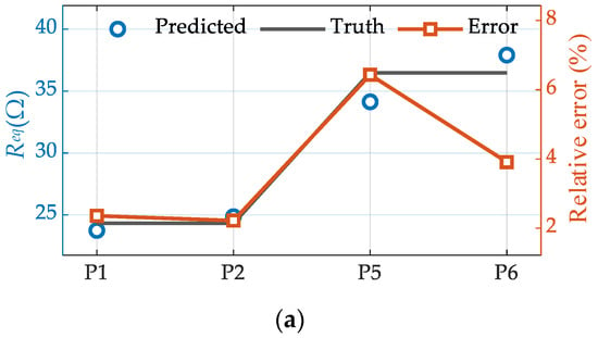
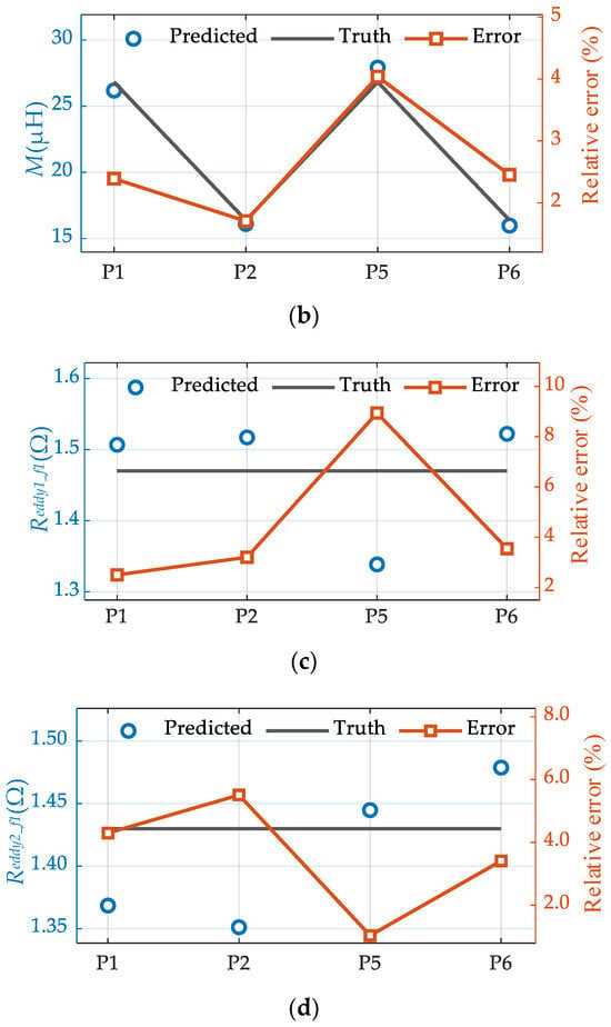
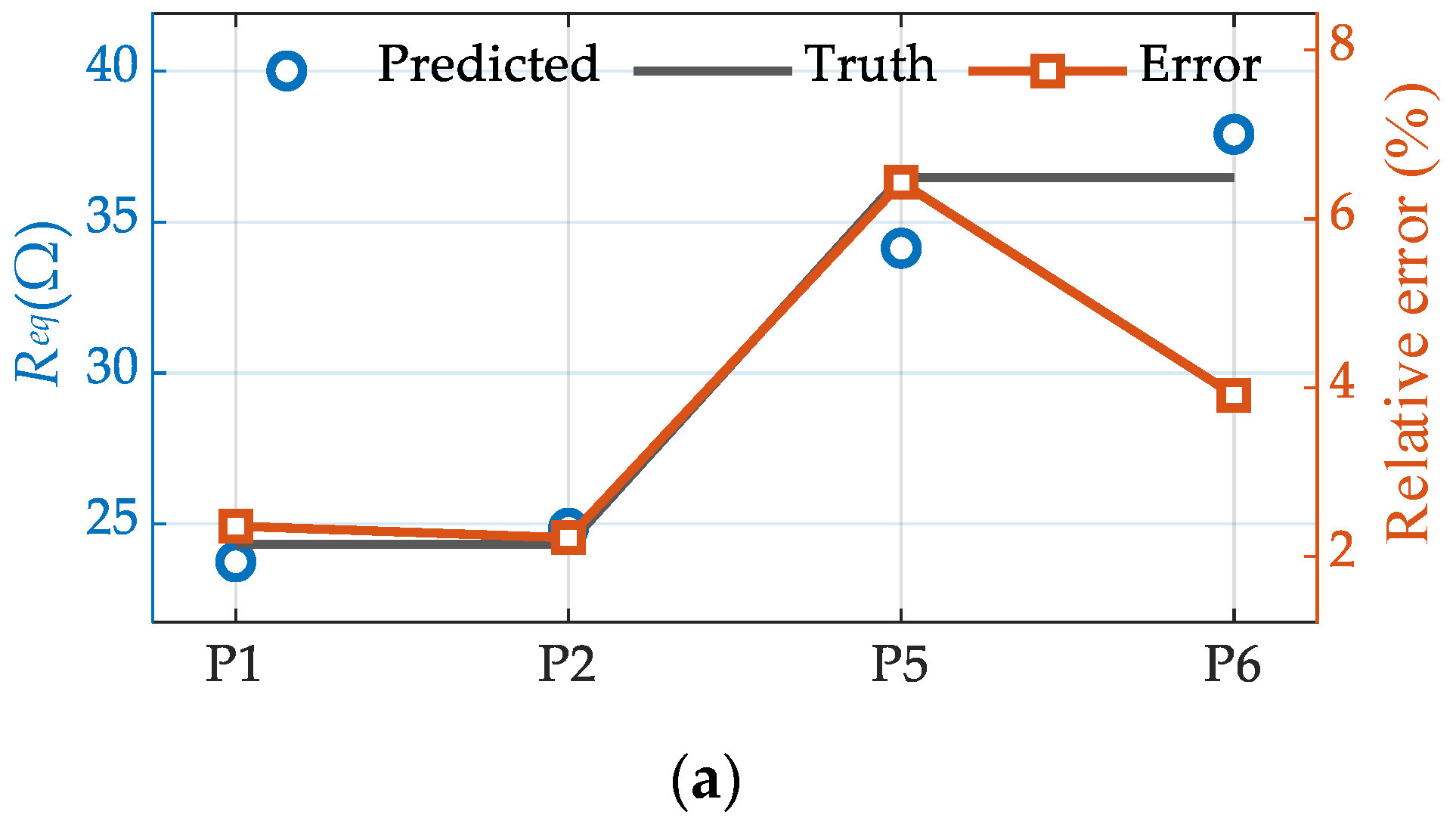
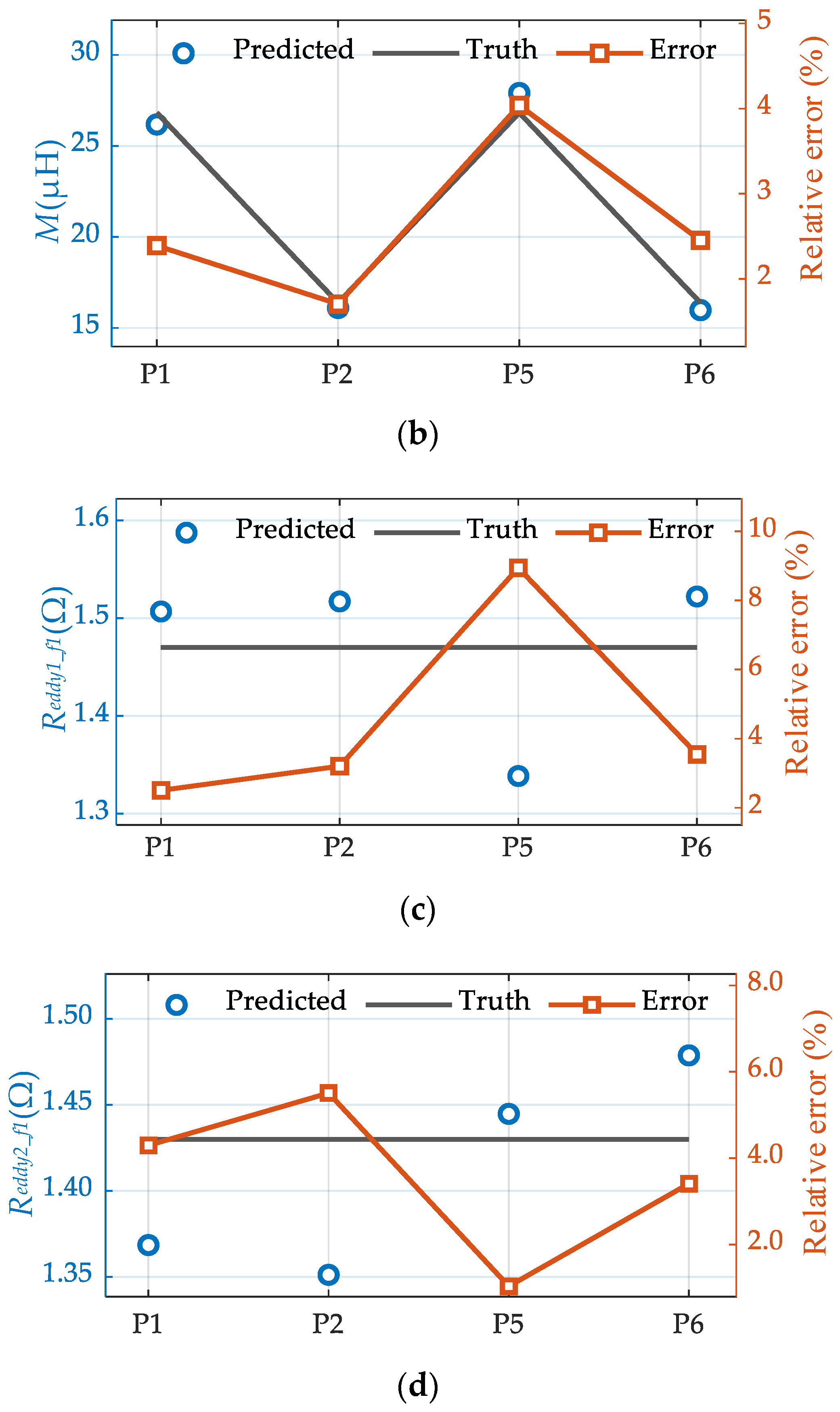
Among them, Figure 14a–d show the identification results of R_eq, M, R_{eddy1_f1}, and R_{eddy2_f1}, respectively.

Figure 14. Identification results when R_{eddy1_f1} = 1.47 Ω, R_{eddy2_f1} = 1.45 Ω: (a) Relationship between R_eq and Relative error; (b) Relationship between M and Relative error; (c) Relationship between R_{eddy1_f1} and Relative error; (d) Relationship between R_{eddy2_f1} and Relative error.

The results indicate that the proposed method can provide stable and consistent parameter estimates under both coil spacing variations and load changes. The fitness function remains close to one, suggesting a small deviation between the impedance magnitudes calculated by the theoretical model and those measured experimentally. Among the identified parameters, M shows the highest accuracy, because it has the most distinct influence on the input impedance. Since it appears in the reflected impedance term as ω²M², small variations in M produce noticeable changes in the impedance response, which improves its identifiability. In contrast, R_{eddy1_f1} and R_{eddy2_f1} act mainly as series resistive terms and affect the impedance magnitude in a similar manner. Their contributions are therefore more difficult to separate, leading to relatively larger identification errors. Nevertheless, the maximum relative error is kept within 5%, demonstrating that the method maintains good robustness and practical applicability across different operating conditions.

4.3. Identification Experiments Under Varying Dielectric Conductivity

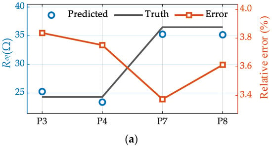
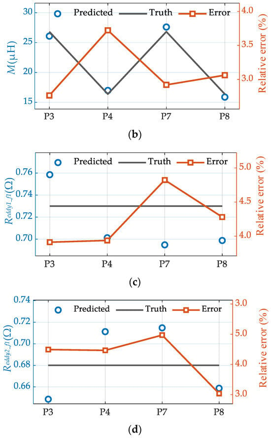
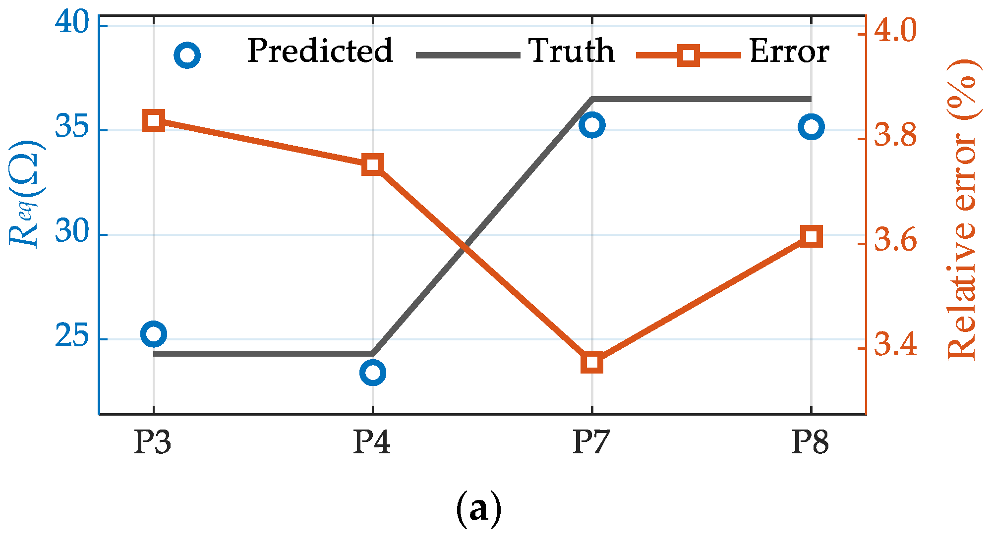
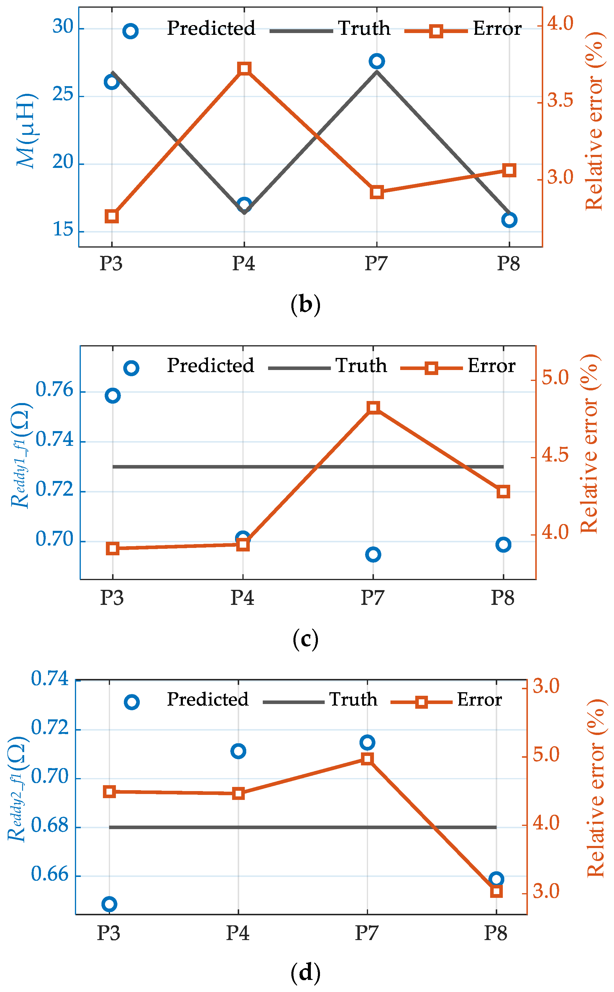
Based on Section 4.2, this section further evaluates the proposed method’s capability to identify eddy-current loss related parameters under varying environmental conditions. The RMS values of the port voltage and current were acquired at two frequency points, 120 kHz and 50 kHz, as listed in Table 4, and parameter identification was conducted for four operating cases (P3, P4, P7, and P8), respectively. By comparing the estimated results across different operating cases and frequency points, we assess the parameter separability and identification stability enabled by introducing a frequency-dependent constraint on the eddy-current loss equivalent resistance under amplitude only measurements. This analysis verifies that changes in the eddy-current loss equivalent resistance can be reliably captured while avoiding estimation interference with M and R_eq.

Table 4. System operating conditions.

Conditions	120 kHz				50 kHz
	Uin1	Iin1	Uin2	Iin2	Uin1	Iin1	Uin2	Iin2
P3	89.99	12.16	141.64	2.60	89.99	10.18	170.08	2.64
P4	89.99	11.82	135.15	2.27	89.99	10.13	169.69	2.61
P7	89.99	12.12	141.05	2.57	89.99	10.17	169.96	2.63
P8	89.99	11.91	135.68	2.21	89.99	10.14	169.68	2.60

Figure 15a–d show the identified results of R_eq, M, R_{eddy1_f1}, and R_{eddy2_f1}, respectively.

Figure 15. Identification results when R_{eddy1_f1} = 0.73 Ω, R_{eddy2_f1} = 0.70 Ω: (a) Relationship between R_eq and Relative error; (b) Relationship between M and Relative error; (c) Relationship between R_{eddy1_f1} and Relative error; (d) Relationship between R_{eddy2_f1} and Relative error.

As the medium conductivity increases, the underwater eddy-current effect becomes more pronounced, and the corresponding equivalent resistance representing eddy-current loss in the system increases accordingly. Because the proposed identification model incorporates a frequency-dependent constraint on the eddy-current loss equivalent resistance, the method can effectively capture the conductivity dependent trend and maintain relatively stable identification accuracy across different conductivity conditions. The experimental results indicate that the proposed approach exhibits a degree of robustness to conductivity variations in underwater environments caused by factors such as salinity and temperature, and is therefore suitable for parameter identification in practical seawater conditions.

4.4. Algorithm Comparison

Based on the analysis results presented in Section 4.2 and Section 4.3, the average operating parameters under two sets of experimental conditions are summarized in Table 5. This table further compiles the mean relative errors of the parameters M, R_eq, R_{eddy1_f1}, and R_{eddy2_f1} under each operating condition after regrouping, thereby enabling a quantitative evaluation of the parameter identification accuracy of the HPSO.

Table 5. Comparison table of identified parameters and average error.

Conductivity (S/m)	M (μH)	Req (Ω)	Reddy1_f1 (Ω)	Reddy2_f1 (Ω)
6	2.64%	3.73%	4.55%	3.56%
3	3.11%	3.64%	4.24%	4.23%

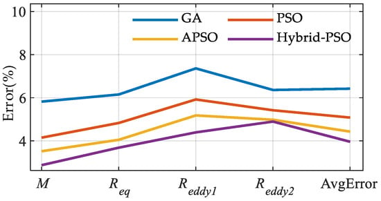
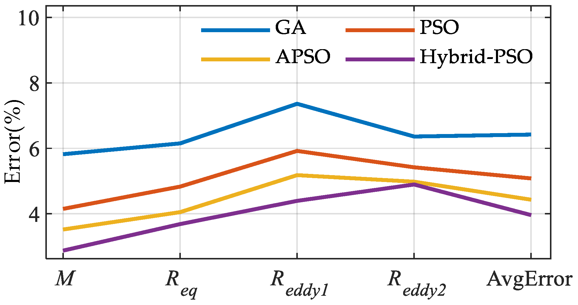
To further highlight the superiority of the proposed HPSO, PSO, GA, and adaptive PSO (APSO), which are widely used for parameter identification in IPT systems, are selected as benchmark methods. Comparative experiments are conducted under eight operating conditions, and the four algorithms are comprehensively evaluated in terms of identification accuracy, convergence speed, and stability.

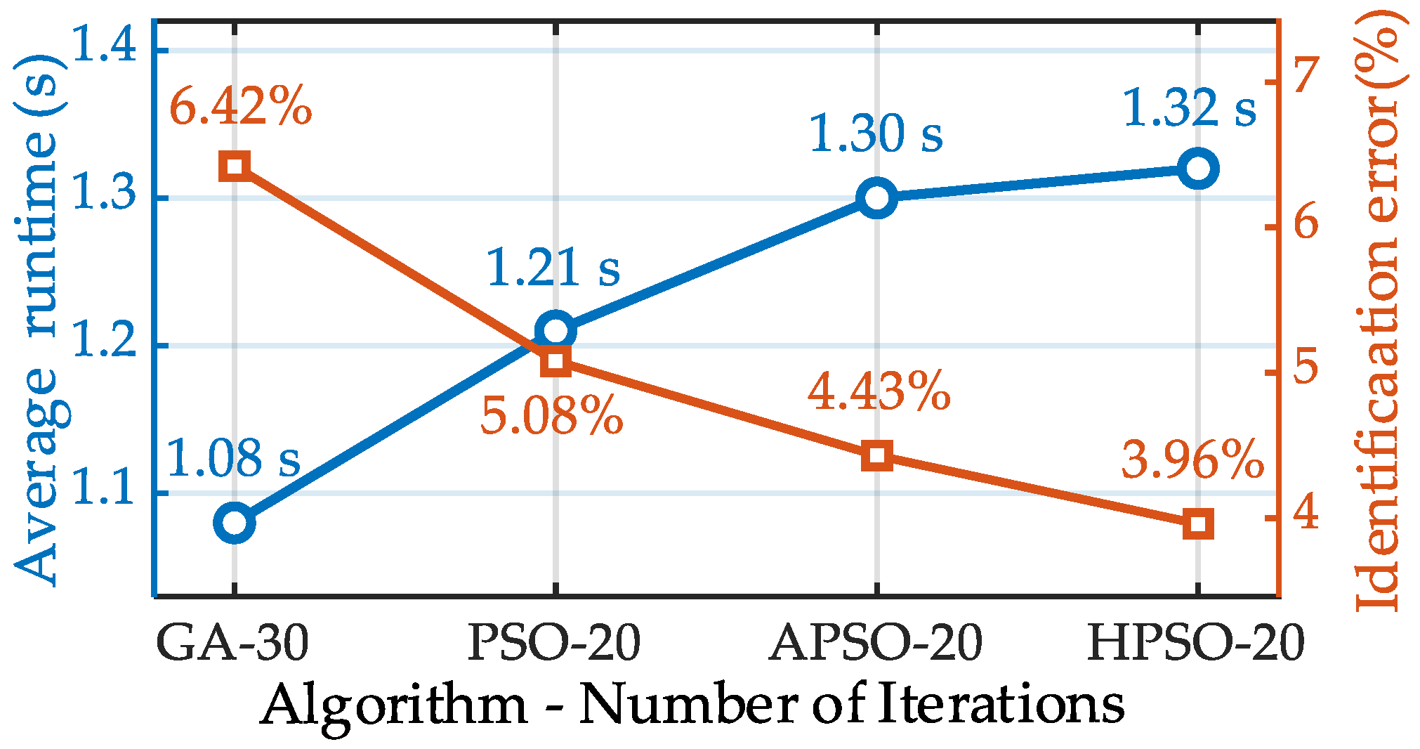
As shown in Figure 16, the proposed HPSO algorithm achieves an overall average identification error of 3.96% across the eight operating conditions, which is lower than that of GA (6.42%), conventional PSO (5.08%), and APSO (4.43%). For the identification of the mutual inductance, equivalent load resistance, and eddy-current-loss equivalent resistance, the proposed method delivers the best or consistently superior overall accuracy, indicating that introducing genetic crossover and mutation operators into the PSO framework can effectively improve the accuracy of parameter estimation.

Figure 16. Identification results of four algorithms.

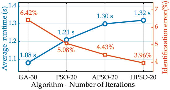
In terms of convergence behavior, PSO and APSO converge rapidly in the early iterations, but they tend to fall into premature convergence. After about 20 iterations, the fitness value shows little further improvement. In contrast, GA exhibits stronger global search capability, but its convergence is slower and generally requires more than 30 iterations to reach a steady state. However, convergence behavior alone is insufficient for a comprehensive evaluation of the algorithms. Therefore, the average runtime and the overall average identification error are further compared, as shown in Figure 17. The results show that GA has the shortest runtime of 1.08 s, followed by PSO (1.21 s) and APSO (1.30 s), whereas HPSO requires 1.32 s. The slightly longer runtime of HPSO is mainly due to the additional crossover and mutation operations introduced into the PSO iteration process.

Figure 17. Comparison of average runtime and overall average identification error of the four algorithms.

Figure 17 shows that HPSO achieves the lowest overall average identification error, although it requires the longest runtime. Since the proposed method is intended for offline parameter identification, this trade-off is acceptable.

Furthermore, to evaluate the consistency of the algorithms over multiple independent runs, the standard deviation of the identification error across 10 independent runs is adopted as the stability metric, as defined in (29).

$$\sigma =\sqrt{{\displaystyle \frac{1}{n}}{\displaystyle \sum _{i=1}^n{\left(x_i-\overline{x}\right)}^2}}$$

(29)

where σ denotes the standard deviation of the identification error, n = 10 is the number of repeated runs, x_i is the relative identification error in the i-th run, and $\overline{x}$ is the mean relative identification error over the n.

According to (29), the standard deviation obtained by HPSO is 0.60, which is lower than those of GA (0.66), conventional PSO (0.63), and APSO (0.61). Considering identification accuracy, runtime, and stability, HPSO demonstrates the best overall performance in the multi-parameter identification of underwater IPT systems. Therefore, HPSO is more suitable for this task than GA, PSO, and APSO.

5. Conclusions

This paper has presented a multi-parameter identification method for underwater DLCC-IPT systems considering the frequency-dependent characteristic of seawater-induced eddy-current loss. Since the equivalent resistance associated with eddy-current loss varies with operating frequency, neglecting this effect in the identification model may lead to noticeable estimation errors, especially under varying underwater environmental conditions.

To overcome this problem, an equivalent circuit model incorporating eddy-current loss frequency dependence was established, and the input impedance expressions at two operating frequencies were derived. By introducing the constraint relationship of the eddy-current loss equivalent resistance at different frequencies, the identification of mutual inductance, equivalent load resistance, and eddy-current loss resistances was formulated as a bounded optimization problem. On this basis, a hybrid particle swarm optimization algorithm was adopted to solve the parameter estimation problem by minimizing the mismatch between the measured and theoretical impedance magnitudes.

The simulation and experimental results demonstrate that the proposed method achieves accurate and stable parameter identification under different coil spacings, load conditions, and medium conductivities, with the maximum relative error maintained within 5%. Compared with GA, PSO, and APSO, the proposed HPSO exhibits superior overall accuracy and stability, which verifies its effectiveness for communication free parameter monitoring in underwater IPT systems.

Nevertheless, the present work still has room for further development. In future research, real-time embedded implementation will be explored to support online identification and closed-loop system regulation. In addition, AI-based or hybrid data-model-driven approaches may be introduced to improve convergence efficiency and robustness under more complex non-linear and time-varying underwater conditions. Furthermore, the proposed identification framework can be generalized to other compensation topologies, such as SS, LCC-S, and other resonant WPT structures, thereby broadening its applicability to diverse underwater wireless power transfer scenarios.

References

- Yan, Z.; Peng, B.; Wang, J.; Liang, B.; Zhang, K.; Hu, Y.; Mao, Z. An Underwater Wireless Power Transfer System With Improved Misalignment Tolerance. IEEE J. Emerg. Sel. Top. Power Electron. 2025, 13, 4369–4376. [Google Scholar] [CrossRef] [Scilit]
- Liu, Y.; Xiong, M.; Zhang, Q.; Yang, F.; Lan, Y.; Jiang, J.; Song, K. Reconfigurable Wireless Power Transfer System with High Misalignment Tolerance Using Coaxial Antipodal Dual DD Coils for AUV Charging Applications. Energies 2025, 18, 4148. [Google Scholar] [CrossRef] [Scilit]
- Ma, Y.; Liang, B.; Wang, J.; Cheng, B.; Yan, Z.; Dong, M.; Mao, Z. A Novel Hill Climbing-Golden Section Search Maximum Energy Efficiency Tracking Method for Wireless Power Transfer Systems in Unmanned Underwater Vehicles. J. Mar. Sci. Eng. 2024, 12, 1336. [Google Scholar] [CrossRef] [Scilit]
- Yi, Y.; Yao, Z.; Pan, W.; Xie, R.; Cheng, X.; Zhang, Y. An antimisalignment electric vehicle wireless charging system based on two transmitting coils with LCC-S compensation. IEEE Trans. Power Electron. 2026, 41, 3198–3202. [Google Scholar] [CrossRef] [Scilit]
- Rong, E.; Wang, S.; Sun, P.; Xiang, Y.; Ji, H.; Hou, Y.; Chang, S.; Yang, G.; Li, S. Wireless Power Transfer for Maritime Application: A Study on Dual-Medium Capacitive Coupler. IEEE Trans. Power Electron. 2026. [Google Scholar] [CrossRef] [Scilit]
- Pahlavan, S.; Jafarabadi-Ashtiani, S.; Mirbozorgi, S.A. Maze-Based Scalable Wireless Power Transmission Experimental Arena for Freely Moving Small Animals Applications. IEEE Trans. Biomed. Circuits Syst. 2025, 19, 120–129. [Google Scholar] [CrossRef] [Scilit]
- Rong, E.; Sun, P.; Qiao, K.; Zhang, X.; Yang, G.; Wu, X. Six-Plate and Hybrid-Dielectric Capacitive Coupler for Underwater Wireless Power Transfer. IEEE Trans. Power Electron. 2024, 39, 2867–2881. [Google Scholar] [CrossRef] [Scilit]
- Pahlavan, S.; Shooshtari, M.; Jafarabadi Ashtiani, S. Star-Shaped Coils in the Transmitter Array for Receiver Rotation Tolerance in Free-Moving Wireless Power Transfer Applications. Energies 2022, 15, 8643. [Google Scholar] [CrossRef] [Scilit]
- Liu, Y.; Sun, P.; Sun, J.; Xiao, Z.; Wang, L.; Li, Y.; Deng, Q. Constant Current/Voltage Charging Control for Communication-Free IPT Systems via Network-Based Deep Transfer Learning. IEEE Trans. Power Electron. 2026, 41, 7118–7133. [Google Scholar] [CrossRef] [Scilit]
- Zhou, Y.; Qiu, M.; Wang, Q.; Ma, Z.; Sun, H.; Zhang, X. Research on Double LCC Compensation Network for Multi-Resonant Point Switching in Underwater Wireless Power Transfer System. Electronics 2023, 12, 2798. [Google Scholar] [CrossRef] [Scilit]
- Li, J.; Zhang, K.; Yan, Z.; Wen, H.; Peng, B.; Wang, J. A Compact Underwater WPT System With Load-Independent Current Output Characteristic Under Wide Range of Coupling Coefficient. IEEE Trans. Power Electron. 2025, 40, 10198–10208. [Google Scholar] [CrossRef] [Scilit]
- Zhang, Y.; Wu, J.; Liu, C.; Tang, H.; Mao, X.; Yin, F.; Tang, Y. Overview of underwater wireless power transfer based on magnetic coupling. Ocean 2025, 1, 9470008. [Google Scholar] [CrossRef] [Scilit]
- Liu, Y.; Madawala, U.K.; Mai, R.; He, Z. Primary-Side Parameter Estimation Method for Bidirectional Inductive Power Transfer Systems. IEEE Trans. Power Electron. 2021, 36, 68–72. [Google Scholar] [CrossRef] [Scilit]
- Dai, X.; Sun, Y.; Tang, C.; Wang, Z.; Su, Y.; Li, Y. Dynamic parameters identification method for inductively coupled power transfer system. In Proceedings of the 2010 IEEE International Conference on Sustainable Energy Technologies (ICSET), Kandy, Sri Lanka, 6–9 December 2010; pp. 1–5. [Google Scholar] [CrossRef] [Scilit]
- Yazdi, S.S.H.; Shafiei, S.; Kapanov, A.; Kermani, M.; Hajizadeh, A.; Bagheri, M. Analyzing Sea Environment’s Effects on Inductive Power Transfer Systems: Equivalent Circuit Parameters and Performance Analysis. In Proceedings of the 2024 IEEE International Conference on Environment and Electrical Engineering and 2024 IEEE Industrial and Commercial Power Systems Europe (EEEIC/I&CPS Europe), Rome, Italy, 17–20 June 2024; pp. 1–6. [Google Scholar] [CrossRef] [Scilit]
- Wang, L.; Sun, P.; Liang, Y.; He, L.; Wu, X.; Deng, Q. Research on the Control Strategy of Communication-Free IPT System Based on Multiparameter Joint Real-Time Identification. IEEE Trans. Power Electron. 2024, 39, 1912–1926. [Google Scholar] [CrossRef] [Scilit]
- Su, Y.-G.; Zhang, H.-Y.; Wang, Z.-H.; Hu, A.P.; Chen, L.; Sun, Y. Steady-State Load Identification Method of Inductive Power Transfer System Based on Switching Capacitors. IEEE Trans. Power Electron. 2015, 30, 6349–6355. [Google Scholar] [CrossRef] [Scilit]
- Lee, S.; Lee, S.-H. Observer-Based Online Parameter Identification of Series–Series Tuned Inductive Power Transfer System. IEEE Trans. Ind. Electron. 2025, 72, 2927–2937. [Google Scholar] [CrossRef] [Scilit]
- Yue, K.; Liu, Y.; Fu, M.; Liang, J.; Wang, H. Mode Switching Based Parameter Identification for 2TX-1RX Wireless Power Transfer Systems. IEEE Access 2023, 11, 46847–46859. [Google Scholar] [CrossRef] [Scilit]
- Sheng, X.; Shi, L. Mutual Inductance and Load Identification Method for Inductively Coupled Power Transfer System Based on Auxiliary Inverter. IEEE Trans. Veh. Technol. 2020, 69, 1533–1541. [Google Scholar] [CrossRef] [Scilit]
- Yin, J.; Lin, D.; Parisini, T.; Hui, S.Y. Front-End Monitoring of the Mutual Inductance and Load Resistance in a Series–Series Compensated Wireless Power Transfer System. IEEE Trans. Power Electron. 2016, 31, 7339–7352. [Google Scholar] [CrossRef] [Scilit]
- Lin, D.; Yin, J.; Hui, S.Y.R. Parameter identification of wireless power transfer systems using input voltage and current. In Proceedings of the 2014 IEEE Energy Conversion Congress and Exposition (ECCE), Pittsburgh, PA, USA, 14–18 September 2014; pp. 832–836. [Google Scholar] [CrossRef] [Scilit]
- Yang, Y.; Tan, S.-C.; Hui, S.Y.R. Front-End Parameter Monitoring Method Based on Two-Layer Adaptive Differential Evolution for SS-Compensated Wireless Power Transfer Systems. IEEE Trans. Ind. Inform. 2019, 15, 6101–6113. [Google Scholar] [CrossRef] [Scilit]
- Yang, Y.; Tan, S.C.; Hui, S.Y.R. Fast Hardware Approach to Determining Mutual Coupling of Series–Series-Compensated Wireless Power Transfer Systems With Active Rectifiers. IEEE Trans. Power Electron. 2020, 35, 11026–11038. [Google Scholar] [CrossRef] [Scilit]
- Zhao, J.; Li, L.; Wang, T.; Wu, H.; Luo, B.; Li, H.; Zhang, Y.; Liu, S.; Zhao, L.; Huang, L. Multi-Parameter Identification Method for Underwater Wireless Power Transfer Based on Adaptive Particle Swarm Optimization Algorithm. In Proceedings of the 2025 IEEE 20th Conference on Industrial Electronics and Applications (ICIEA), Yantai, China, 3–6 August 2025; pp. 1–6. [Google Scholar] [CrossRef] [Scilit]
- Zhou, J.; Yao, P.; Chen, Y.; Guo, K.; Hu, S.; Sun, H. Design Considerations for a Self-Latching Coupling Structure of Inductive Power Transfer for Autonomous Underwater Vehicle. IEEE Trans. Ind. Appl. 2021, 57, 580–587. [Google Scholar] [CrossRef] [Scilit]
- Sun, P.; Wu, X.; Cai, J.; Wang, X.; Zhang, X.; Liang, Y.; Xiong, Q.; Rong, E. Eddy current loss analysis and frequency optimization design of double-sided LCC-IPT system in seawater environment. Sci. China Technol. Sci. 2022, 65, 12. [Google Scholar] [CrossRef] [Scilit]
- Zhang, K.; Ma, Y.; Yan, Z.; Di, Z.; Song, B.; Hu, A.P. Eddy Current Loss and Detuning Effect of Seawater on Wireless Power Transfer. IEEE J. Emerg. Sel. Top. Power Electron. 2020, 8, 909–917. [Google Scholar] [CrossRef] [Scilit]
- Yu, L.; Sun, H.; Su, S.; Tang, H.; Sun, H.; Zhang, X. Review of Crucial Problems of Underwater Wireless Power Transmission. Electronics 2023, 12, 163. [Google Scholar] [CrossRef] [Scilit]
- Chen, Z.; Yang, Q.; Zhang, X.; Xu, F.; Deng, X.; Wei, Y.; Liu, J.; Tse, C.K. Hybrid Mechanism- and Data-Driven Joint Parameter Identification for Underwater Wireless Power Transfer Systems. IEEE Trans. Power Electron. 2026, 41, 6967–6980. [Google Scholar] [CrossRef] [Scilit]
- Liu, X.; Lu, D.; Liao, Z.; Rong, C.; Xia, C. Critical and Parasitic Parameters Identification and Frequency Regulation Strategies for UWPT Systems. IEEE Trans. Power Electron. 2024, 39, 10558–10567. [Google Scholar] [CrossRef] [Scilit]
- Li, T.; Wang, Y.; Liu, Z.; Sun, Z.; Tian, W.; Cui, J.; Mai, J.; Xu, D. Identification of Multiple Critical Parameters in Undersea Wireless Power Transfer System Integrating Primary-Side Phase Acquisition. IEEE Trans. Power Electron. 2026, 41, 7220–7232. [Google Scholar] [CrossRef] [Scilit]
- Zhao, Y.; Guo, X.; Yin, F.; Zhang, Y. Optimized Parameter Identification and Frequency Control Methods for Misalignment-Tolerant UWPT Systems Based on Primary-Side Feedback. IEEE Trans. Transp. Electrif. 2026, 12, 499–514. [Google Scholar] [CrossRef] [Scilit]
Disclaimer/Publisher’s Note: The statements, opinions and data contained in all publications are solely those of the individual author(s) and contributor(s) and not of MDPI and/or the editor(s). MDPI and/or the editor(s) disclaim responsibility for any injury to people or property resulting from any ideas, methods, instructions or products referred to in the content. |
© 2026 by the authors. Licensee MDPI, Basel, Switzerland. This article is an open access article distributed under the terms and conditions of the Creative Commons Attribution (CC BY) license.