Highly Non-Uniform Stripe Ionospheric Clutter Suppression Algorithm for HFSWR

Abstract

High-frequency surface wave radar (HFSWR) often suffers from highly non-uniform, striped ionospheric clutter, which significantly degrades sea-surface target detection performance. To address this challenge, this paper proposes a reduced-dimension space-time adaptive processing (STAP) algorithm based on sparse representation. In this method, a dictionary is first constructed using the Doppler resolution and an appropriate angle interval as the frequency and angle grids, aiming to obtain fully orthogonal clutter atoms. Both the training sample and the cell under test are then sparsely represented over this dictionary to extract consistent clutter atoms. Due to discrepancies between the dictionary atoms and the actual clutter, low-power atoms are deemed unreliable and are discarded via a thresholding procedure. The remaining reliable atoms are used to construct a dimensionality-reduction matrix, thereby obtaining an accurate local clutter-plus-noise covariance matrix. Experimental results on measured data demonstrate that the proposed method effectively suppresses striped ionospheric clutter and enhances target detection performance.

1. Introduction

High-frequency surface wave radar (HFSWR) is widely used for maritime surveillance due to its ability to detect ship targets over long distances by exploiting electromagnetic waves that propagate along the Earth’s surface. Since sea-surface target echoes are typically weak, coherent accumulation of a large number of pulses is required to improve the signal-to-clutter ratio, resulting in long integration times. In addition, HFSWR systems generally employ multiple receiving antenna elements and perform multi-pulse sampling at each element, generating high-dimensional space-time echo data. Meanwhile, HFSWR is often affected by striped ionospheric clutter, which primarily originates from sporadic Es-layer scatterers. This clutter is characterized by high power, occupancy of a limited number of range cells, and pronounced spatial non-uniformity, severely degrading target detection performance [1,2,3].

To effectively mitigate ionospheric clutter, the most widely recognized and effective approach is space-time adaptive processing (STAP), which suppresses clutter while preserving target signals by jointly filtering in both the spatial and temporal domains. Brennan et al. first proposed the fundamental theory of STAP [4]. In STAP, when clutter-plus-noise follows a complex Gaussian distribution, the sample covariance matrix estimated from a finite number of snapshots follows a complex Wishart distribution [4]. This imposes two key requirements on STAP: (a) The training samples must be independent and identically distributed (IID) with the cell under test (CUT). (b) To ensure that the average signal-to-clutter-plus-noise ratio (SCNR) loss is less than 3 dB, at least 2 × M × N training samples are required, where M and N denote the number of pulses and array elements, respectively.

The full-dimension STAP algorithm based on sparse representation of the clutter-plus-noise covariance matrix can effectively suppress clutter even with a single training sample [5]. However, it has two major limitations. First, the algorithm performance degrades significantly when the training sample is highly non-uniform with respect to the cell under test. Second, STAP requires inverting the full-dimension clutter-plus-noise covariance matrix. The space-time dimension of HFSWR is typically very large, resulting in an extremely high computational load that is difficult to process in real time. Furthermore, when performing the matrix inversion, the software employs double-precision storage by default, and the inversion algorithm generates a large number of temporary matrices, each of size MN × MN, which often exceeds the available computer memory.

To improve computational efficiency and reduce memory requirements, various reduced-dimension STAP algorithms have been proposed. These algorithms effectively lower the dimension of the clutter-plus-noise covariance matrix by mapping the data from the space-time domain to the angle-Doppler domain, thereby significantly enhancing their practicality and feasibility. Typical reduced-dimension STAP algorithms include the space time multibeam (STMB) algorithm, the joint domain localized (JDL) algorithm, and the sequential convex programming (SCP) algorithm [6,7,8]. However, all of these algorithms require a large number of training samples to estimate the clutter covariance matrix, and their performance degrades significantly when only a single training sample is available.

To suppress ionospheric clutter, this paper presents a novel reduced-dimension STAP approach based on sparse representation [9,10,11]. Specifically, a dictionary is first constructed using the Doppler resolution and an appropriate angular interval as the frequency and angle grids, with the goal of obtaining fully orthogonal clutter atoms. Both the training samples and the cell under test are then sparsely represented over this dictionary to extract consistent clutter atoms. Due to inevitable discrepancies between the dictionary atoms and the actual clutter, low-power atoms are deemed unreliable and eliminated via a thresholding procedure. The remaining reliable atoms are subsequently used to form a dimensionality-reduction matrix, enabling the accurate estimation of the local clutter-plus-noise covariance matrix [12,13,14,15].

The organization of this paper is as follows. Section 2 introduces the HFSWR clutter model. The proposed channel selection algorithm is derived in Section 3. Simulations and performance analysis of the proposed algorithm are presented in Section 4, and conclusions are provided in Section 5.

2. Clutter Model

HFSWR employs vertically polarized antennas to transmit electromagnetic waves and utilizes ground-wave propagation and sea-surface diffraction to achieve long-range maritime target detection. However, due to the limited size of the HFSWR transmitting antenna panels, ground losses, and the finite width of the antenna’s E-plane beam, the antenna’s main lobe is inclined upward at a certain angle. Consequently, in addition to diffraction along the sea surface, part of the high-frequency electromagnetic energy is radiated into the upper half-space at a certain elevation angle. After interacting with the ionosphere, this energy returns to the radar along multiple paths, causing significant interference [16,17,18,19,20].

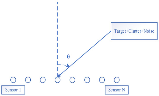
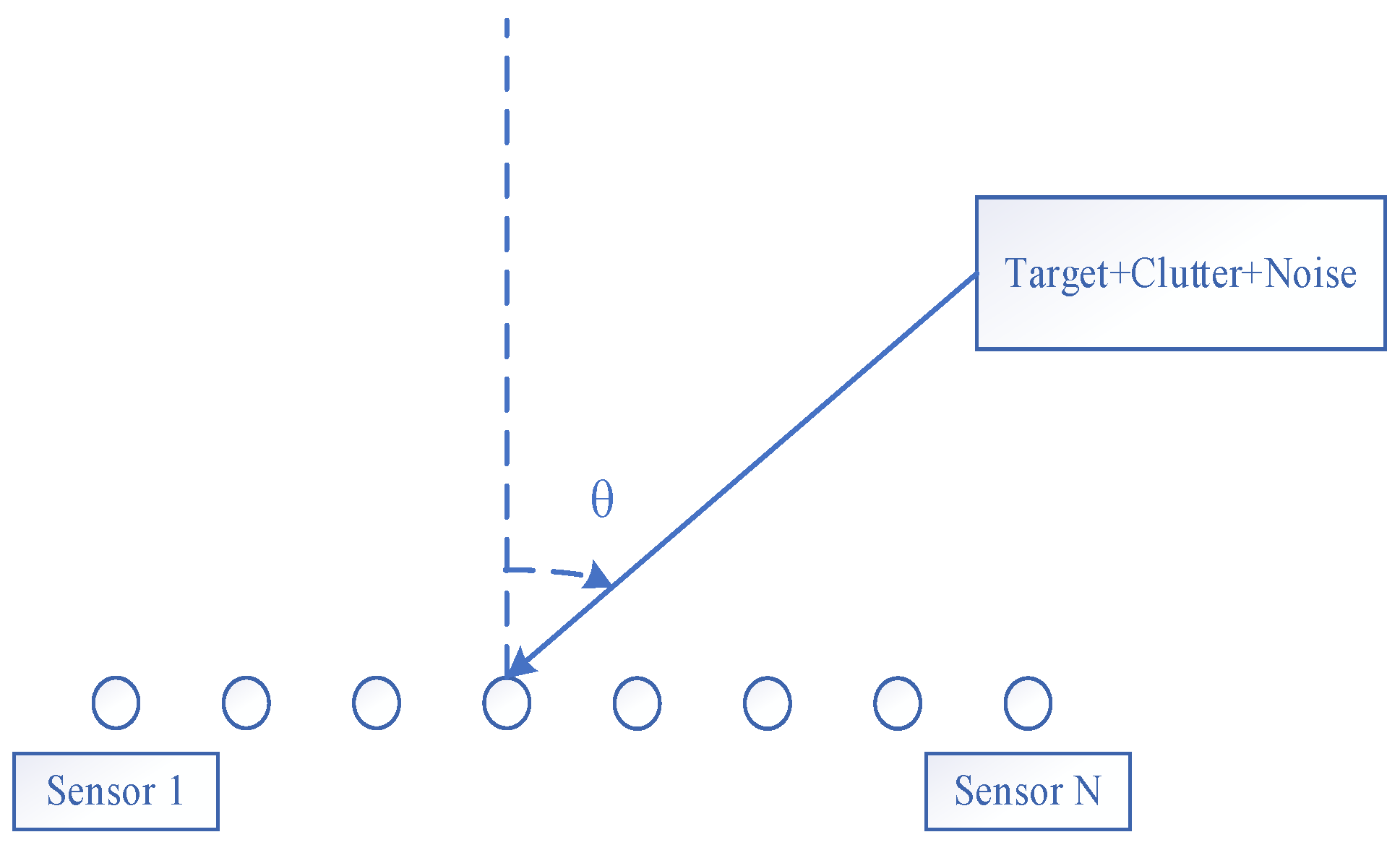
The measured data used in this study were collected on 7 August 2018, at the Weihai radar station in Shandong Province, China. For the sake of subsequent discussion, this study first introduces the basic characteristics of the radar station. The radar is located in a coastal region of Shandong Province, China, and is primarily used for observing maritime vessels. The radar employs a 32 antenna uniform linear array (ULA) antenna configuration for detection. Each coherent processing interval (CPI) consists of 4480 pulses. The antenna configuration is represented in Figure 1.

Figure 1. Array configuration.

• where θ denotes the incident direction of the ionospheric clutter or the signal. The CUT and training sample can be represented as follows:

$$\begin{array}{l}{\mathit{X}}_{cut}={\mathit{a}}_s\mathit{S}+{\mathit{C}}_{cut}+\mathit{N},\\ {\mathit{X}}_{ts}={\mathit{C}}_{ts}+\mathit{N},\end{array}$$

(1)

where X_cut represents the data in the CUT, a_s denotes the target amplitude, S is the target, C_cut is the ionospheric clutter, and N is the Gaussian noise. The target S is represented in the form of a space-time steering vector.

$$\begin{array}{l}\mathit{S}=\mathit{a}(\theta )\otimes \mathit{a}(f_d),\\ \mathit{a}(\theta )=[\begin{array}{c}1 e^{2\pi jd\sin (\theta )/\lambda } \cdots e^{2\pi j(N-2)d\sin (\theta )/\lambda } e^{2\pi j(N-1)d\sin (\theta )/\lambda }\hfill \end{array}],\\ \mathit{a}(f_d)=[\begin{array}{c}1 e^{2\pi j{f}_d{T}_r} \cdots e^{2\pi j(M-2)f_d{T}_r} e^{2\pi j(M-1)f_d{T}_r}\hfill \end{array}],\end{array}$$

(2)

where $\otimes$ denotes the Kronecker product, a(θ) represents the spatial steering vector, N denotes the number of antennas, d denotes the antenna spacing, θ is the incident angle, λ is the wavelength, a(f_d) represents the time steering vector, and M denotes the number of pulses. f_d denotes the Doppler frequency, and T_r represents the pulse repetition interval (PRI).

2.1. Space-Time Steering Vector Representation of Ionospheric Clutter

The angle and Doppler frequency resolutions of HFSWR are crucial for the subsequent construction of the sparse representation dictionary D. Moreover, the measurable ranges of angle and Doppler frequency are also of significant importance. Therefore, we first examine these two aspects.

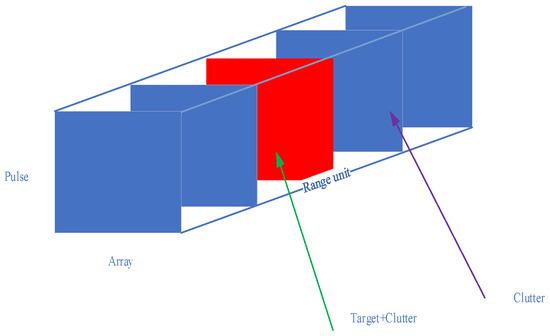
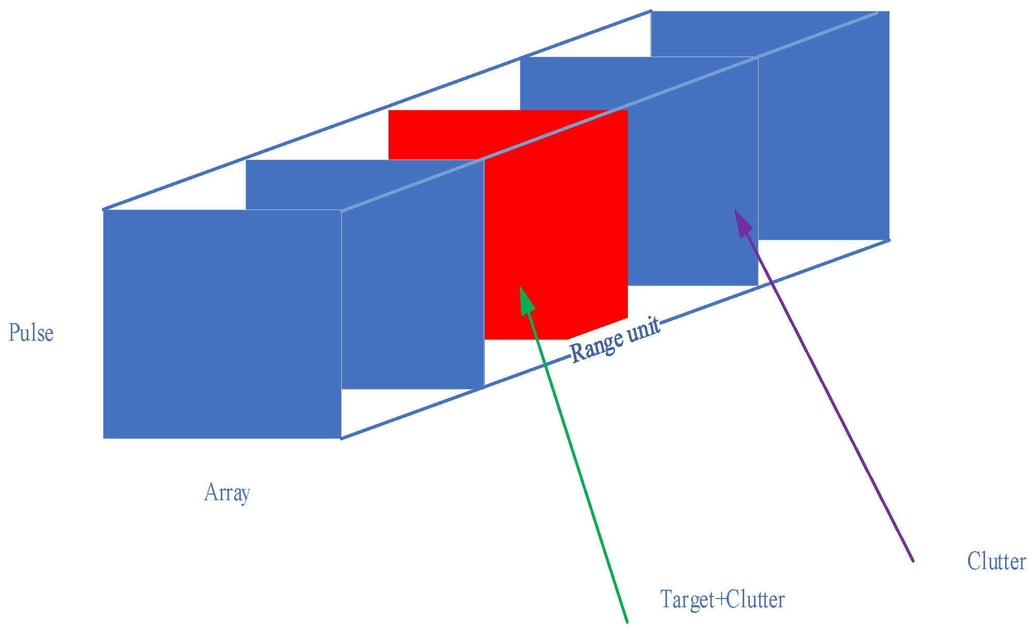
The data after pulse compression have a three-dimensional form, which is intuitively illustrated in Figure 2.

Figure 2. Three-dimensional data storage diagram.

Radar echoes are typically processed as discrete complex signals. After Doppler processing in the time domain, the resulting discrete points correspond to the number of pulses and are arranged at intervals determined by the Doppler frequency resolution. The Doppler frequency resolution is given by the following formula:

$$\Delta f_d={\displaystyle \frac{1}{M{T}_r}},$$

(3)

where M denotes the number of pulses, and T_r represents the pulse repetition interval. The M discrete frequency points after Doppler processing are represented as follows:

$$\mathit{F}={\displaystyle \frac{-M}{2}}\Delta f_d:\Delta f_d:({\displaystyle \frac{M}{2}}-1)\Delta f_d,$$

(4)

where F denotes the Doppler frequency range. Digital beamforming can be regarded as the implementation of the spatial Fourier transform in the discrete angle domain. The spatial resolution of the discrete spatial Fourier transform is expressed as follows:

$$\Delta f_s={\displaystyle \frac{1}{N}},$$

(5)

where Δf_s represents the spatial frequency resolution, which is related to the angle resolution as follows:

$$\begin{array}{l}{f}_s={\displaystyle \frac{d\sin (\theta )}{\lambda }},\\ \Delta \theta ={\displaystyle \frac{0.886\lambda }{Nd\cos (\theta )}},\end{array}$$

(6)

where f_s represents the spatial frequency, and Δθ represents the 3 dB angle resolution. As shown in (6), the angle resolution depends on the incident angle. When the incident direction is 60°, the 3 dB angular resolution is reduced by half. Consequently, the radar’s effective measurement angular range is limited to ±60°.

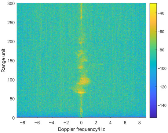
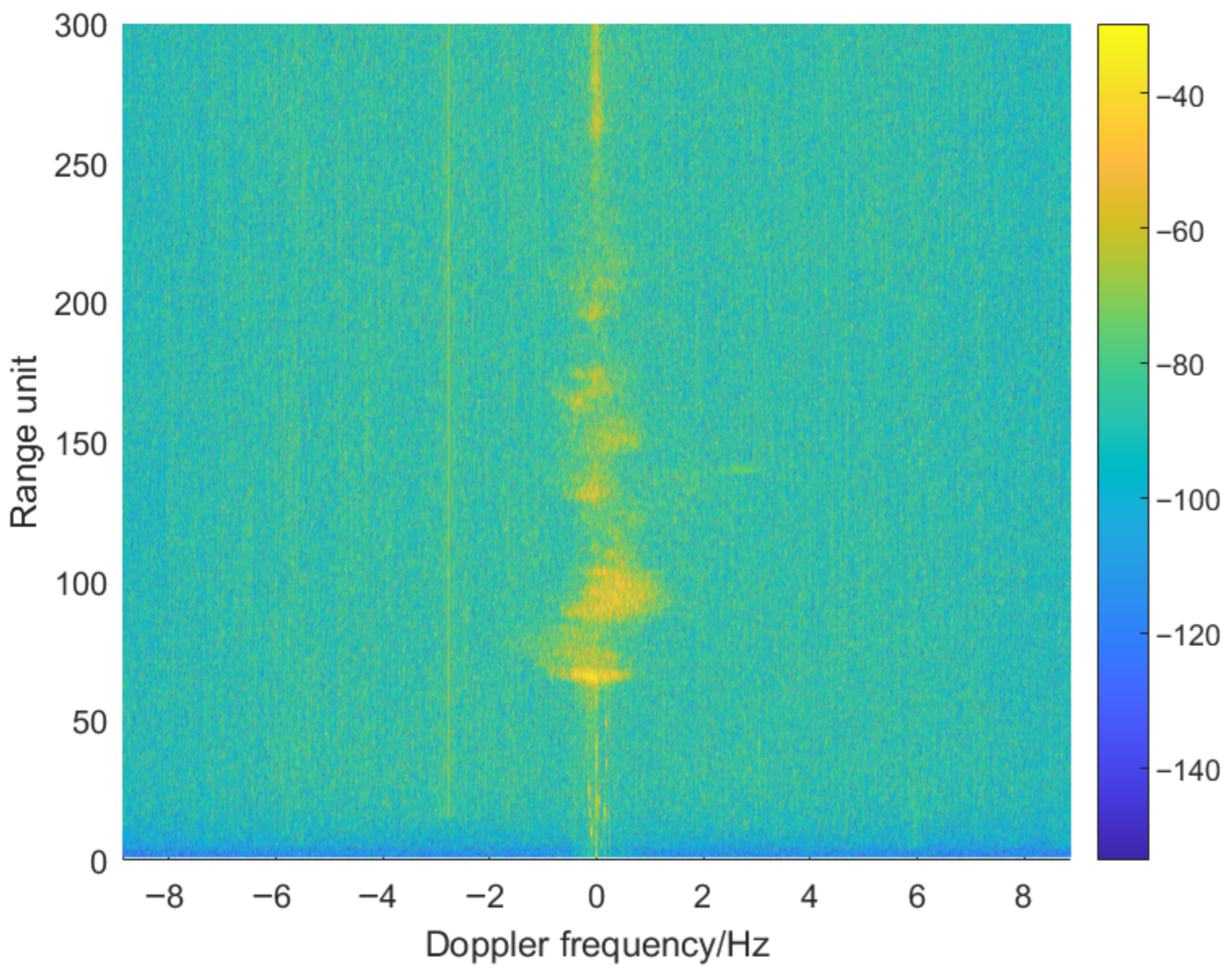
Figure 3 shows a range-Doppler map when the beam is steered at 10°. Due to the wide Doppler frequency range, it is difficult to observe the ships of interest.

Figure 3. Example of a range-Doppler map when the receive beam is steered to 10°.

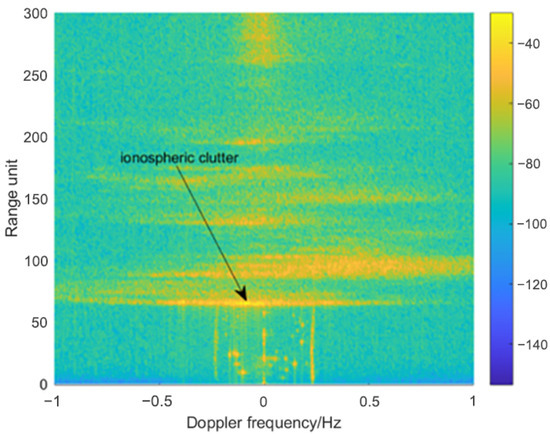
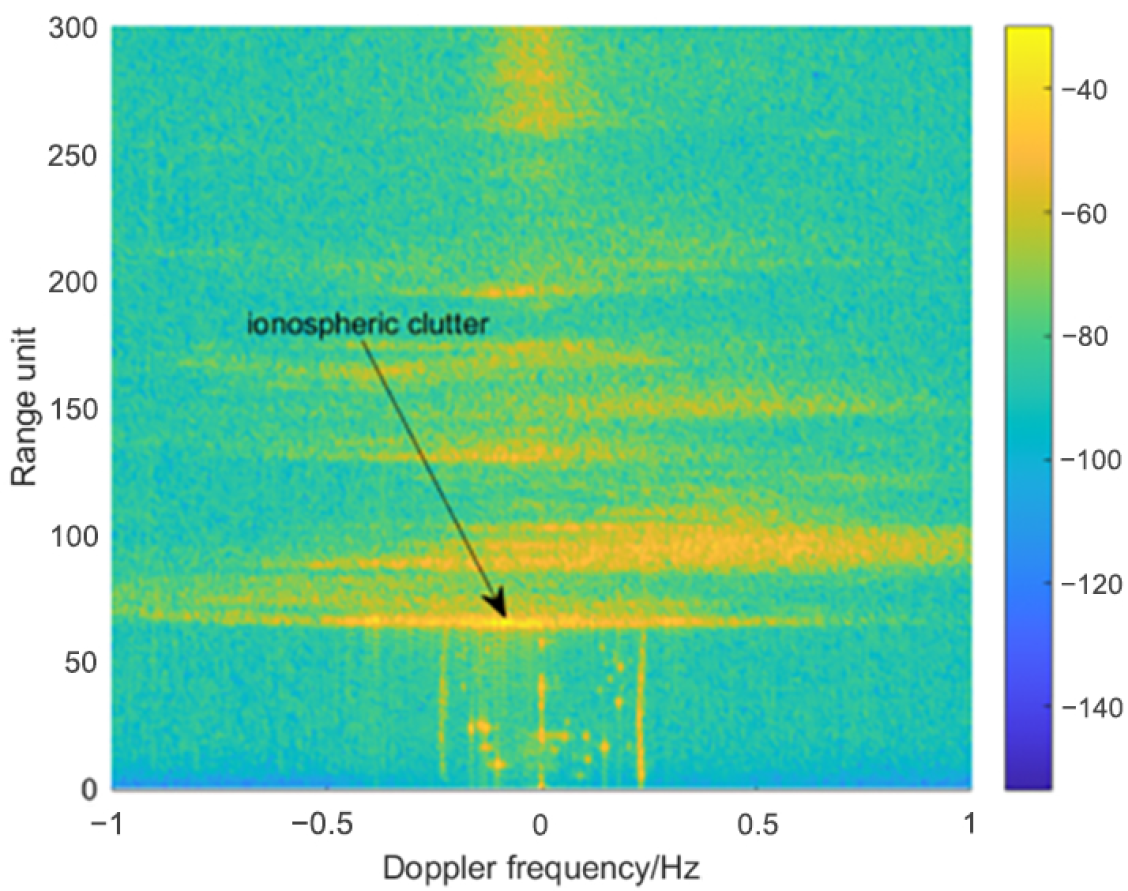
Figure 4 shows the Doppler axis of the range-Doppler plot constrained to ±1 Hz. As shown in Figure 4, the sea clutter components are located at ±0.23 Hz. In HFSWR, the “sea clutter components” generally refer to strong background echoes caused by Bragg scattering from the sea surface. When the wavelength of the incident electromagnetic wave satisfies the Bragg resonance condition with ocean surface waves, coherent interactions occur with both the forward- and backward-propagating wave components. This leads to prominent Doppler spectral peaks, which appear symmetrically around zero frequency and correspond to positive and negative Doppler shifts induced by wave motion along the radar line of sight. These components are therefore observed as the ±Bragg frequency (e.g., ±0.23 Hz), forming the typical structure of sea clutter in the Doppler spectrum [21]. In addition, large-scale ionospheric clutter is distributed beyond the 60th range cell. A strong stripe-like ionospheric clutter appears around the 66th range cell, which is selected as the CUT in this study.

Figure 4. The same range-Doppler map shown in Figure 4 with the Doppler extent limited to ±1 Hz.

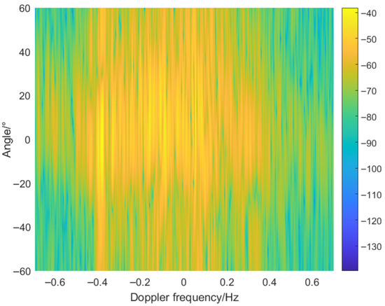
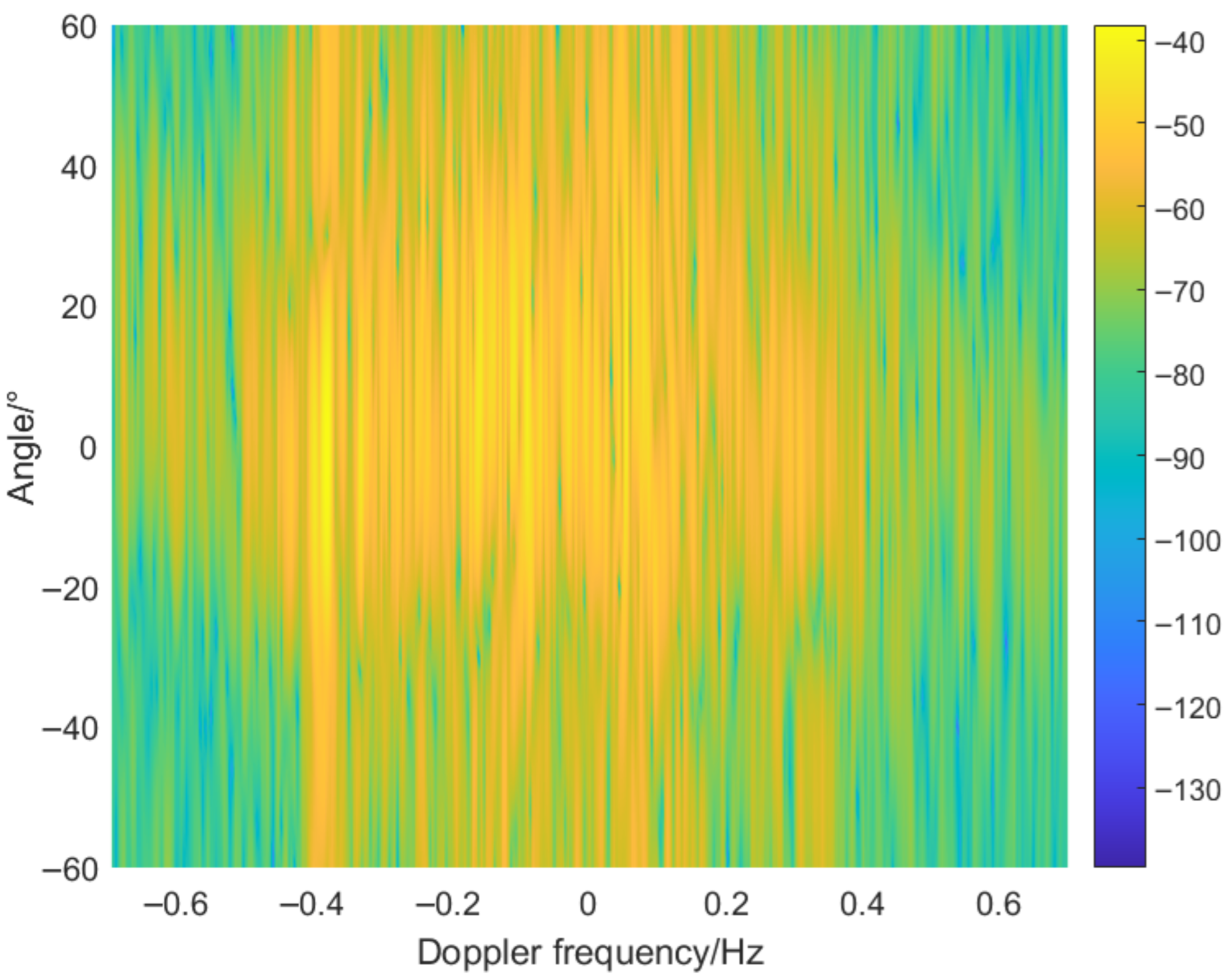
Figure 5 illustrates the angle-Doppler spectrum of the CUT, where the Doppler frequency is likewise restricted to the region of interest. HFSWR is used to detect ships over the sea surface. However, ship echoes are inherently weak. To enhance the SCNR, a long coherent integration time is typically required, which leads to an extremely high Doppler frequency resolution. In this study, 4480 pulses are coherently integrated, resulting in a Doppler resolution of 0.004 Hz.

Figure 5. Angle-Doppler map corresponding to the 66th range cell.

In contrast, the number of antenna elements is only 32, yielding relatively low angle resolution. When the incident angle is 0°, the 3 dB angle resolution is approximately 6.6°.

The CPI used in this study is approximately 4 min. Within such a short time scale, the overall structure of the ionosphere remains essentially stable. Although some small-scale structures exhibit dynamic variations, their impact on the overall scattering characteristics is limited. Therefore, the ionospheric clutter can still be approximated as stationary within this time window. This quasi-stationarity provides a reasonable basis for modeling the clutter using space-time steering vectors, facilitating stable STAP.

2.2. The Construction Method of the Dictionary D

In sparse representation algorithms, the construction of the dictionary D is of critical importance [22,23,24]. Typically, the dictionary is composed of space-time steering vectors, as these vectors closely match the physical model of radar observations. This ensures that both the signal and clutter can be sparsely represented within the dictionary, thereby fully satisfying the fundamental assumptions of sparse representation algorithms [25,26,27].

The dictionary typically needs to cover the angle-Doppler range of clutter and targets. If the angle extent [θ_min, θ_max] is discretized into N_θ points, and the Doppler extent [f_min, f_max] is discretized into N_f points, then the total number of dictionary atoms is N_θ × N_f.

HFSWR exhibits very high Doppler resolution. By constructing the dictionary with intervals equal to the Doppler resolution in (3), each resolvable radial velocity corresponds to a dictionary atom. This approach avoids redundant atoms that increase computational load while maintaining sparse representation accuracy consistent with the radar’s physical resolution, making it the most suitable choice.

$$N_f={\displaystyle \frac{f_{\max }-f_{\min }}{\Delta f_s}},$$

(7)

The 3 dB angle resolution of HFSWR is generally low. If this resolution is directly used as the angular spacing for the dictionary or sparse representation, the resulting angular grid would be too coarse, making it difficult to accurately distinguish targets from clutter and thus degrading the spectral estimation accuracy. To balance resolution and computational complexity, this study adopts an angle spacing of 2°.

$$N_{\theta }={\displaystyle \frac{{\theta }_{\max }-{\theta }_{\min }}{2°}},$$

(8)

In sparse representation, the dictionary D is typically composed of space-time steering vectors. Each column corresponds to an atom, representing a space-time steering vector at a specific angle and Doppler frequency.

$$\begin{array}{l}\mathit{D}={\displaystyle \sum _{i=1}^{N_{\theta }}{\displaystyle \sum _{j=1}^{N_f}\mathit{a}({\theta }_i,f_j)}}\in {\mathit{C}}^{MN\times N_{\theta }{N}_f},\\ \mathit{a}({\theta }_i,f_j)=\mathit{a}({\theta }_i)\otimes \mathit{a}(f_j),\end{array}$$

(9)

From the construction of the discrete dictionary, it can be seen that atoms corresponding to different Doppler frequencies are completely orthogonal. Dictionary atoms corresponding to different Doppler frequencies can be expressed as follows:

$$\begin{array}{l}i\ne j,\\ ⟨\mathit{a}({\theta }_i,f_i),\mathit{a}({\theta }_j,f_j)⟩=(\mathit{a}{({\theta }_i)}^H\mathit{a}({\theta }_j))\otimes (\mathit{a}{(f_i)}^H\mathit{a}(f_j))=(\mathit{a}{({\theta }_i)}^H\mathit{a}({\theta }_j))\otimes 0=0,\end{array}$$

(10)

For atoms corresponding to different Doppler frequencies, since the dictionary atoms are constructed with spacing equal to the Doppler frequency resolution, their inner product is 0.

3. Proposed Method

In conventional reduced-dimension STAP, the space-time data are mapped to the angle-Doppler domain by applying a linear transformation matrix T_F.

$${\mathit{T}}_F=[\mathit{S},\mathit{B}],$$

(11)

where S denotes the space-time steering vector corresponding to the target channel, and B represents the space-time steering vectors associated with other angle-Doppler channels. A key step of reduced-dimension STAP algorithms is the selection of the auxiliary channels B.

Existing auxiliary-channel selection methods for matrix B can be broadly classified into two categories. The first category relies on prior knowledge of clutter distributions to select auxiliary channels, such as the JDL and STMB methods. The second category is developed from the perspective of random signal processing, in which the received data are modeled as random processes and auxiliary channels are constructed based on statistical characteristics or energy-based criteria, such as the SCP and the recursive angle-Doppler channel selection methods. Both types of auxiliary channels require maximum likelihood estimation of the clutter covariance matrix; therefore, their performance generally degrades significantly in single training sample scenarios. The ionospheric clutter in HFSWR is primarily generated by ionospheric backscattering. Since the ionospheric distribution varies across different range cells, the clutter distribution in the CUT can differ significantly from that in neighboring training samples. The ionospheric clutter can be specifically represented as follows:

$$\begin{array}{l}{\mathit{C}}_{cut}={\displaystyle \sum _{i=1}^L{\beta }_i\mathit{a}({\theta }_i,f_i)}+{\displaystyle \sum _{j=1}^P{\beta }_j\mathit{a}({\theta }_j,f_j)},\\ {\mathit{C}}_{ts}={\displaystyle \sum _{i=1}^L{\beta }_i\mathit{a}({\theta }_i,f_i)}+{\displaystyle \sum _{k=1}^G{\beta }_k\mathit{a}({\theta }_k,f_k)},\\ \mathit{a}({\theta }_i,f_i)=\mathit{a}({\theta }_i)\otimes \mathit{a}(f_i),\end{array}$$

(12)

where C_cut represents the ionospheric clutter in the CUT, C_ts represents the ionospheric clutter in the training sample, L denotes the common clutter components, P and G denote the distinct clutter components, and β_i represents the clutter amplitude.

Sparse representation can be formulated as the following optimization problem: given a dictionary, find a coefficient vector that is as sparse as possible, such that the signal can be accurately represented as a linear combination of the dictionary atoms [28].

$$\underset{\mathit{\beta }}{\min }{‖\mathit{\beta }‖}_0 s.t.{‖\mathit{X}-\mathit{D}\mathit{\beta }‖}_2\le \xi ,$$

(13)

where β denotes the sparse coefficients, and D denotes the space-time dictionary. L₀ norm optimization is fundamentally an NP-hard combinatorial problem that cannot be solved directly, and feasible solutions can only be obtained through approximate algorithms. The typical approximation method is the orthogonal matching pursuit (OMP) algorithm.

3.1. OMP Algorithm

The specific steps of the OMP algorithm (Algorithm 1) can be described as follows.

Algorithm 1 OMP Algorithm

Input: dictionary D and data x, Each column of D is denoted by Dj, Dj is the index.

Initialization: residual ${\mathit{r}}_0=\mathit{X}$ and index ${\mathit{b}}_0=\varphi$

Set the iteration condition: continue iterating while the residual r is greater than the noise power. k represents the iteration number.

Step 1: Find the index ${\mathit{b}}_k=\begin{array}{cc}\arg & \underset{{\mathit{D}}_j}{\max }\end{array}\left|⟨{\mathit{r}}_{k-1},{\mathit{D}}_j⟩\right|$

Step 2: Update the index ${\mathit{b}}_k={\mathit{b}}_{k-1}\cup {\mathit{b}}_k$

Step 3: Compute the sparse coefficient ${\mathit{\beta }}_k={(\mathit{D}{(:,b_k)}^H\mathit{D}(:,b_k))}^{-1}\mathit{D}{(:,b_k)}^H{\mathit{r}}_{k-1}$

Step 4: Update the residual ${\mathit{r}}_k={\mathit{r}}_{k-1}-\mathit{D}(:,b_k){\mathit{\beta }}_k$

Terminate the iteration.

We construct a dictionary based on the region surrounding the target, and then apply the OMP algorithm to perform sparse representation for both the CUT and the training samples, and use (14) to select the common clutter components.

$${\mathit{\beta }}_{cut}={\mathit{\beta }}_{ts} s.t.{\mathit{b}}_{cut}={\mathit{b}}_{ts},$$

(14)

where β_cut represents the sparse coefficients of the CUT, β_ts represents the sparse coefficients of the training sample, b_cut denotes the dictionary index of the CUT, and b_ts denotes the dictionary index of the training sample. The common clutter components can be expressed as follows.

$${\mathit{C}}_{same}={\displaystyle \sum _{i=1}^H{\beta }_i\mathit{D}(:,b_i)},$$

(15)

3.2. Threshold Design Strategy

In Step 3 of the OMP algorithm, an orthogonal projection is performed, which can compress the spread spectrum into a concentrated component. Therefore, the clutter atoms obtained after sparse representation are mutually orthogonal.

$$⟨\mathit{D}(:,b_i),\mathit{D}(:,b_j)⟩=0,$$

(16)

The H clutter atoms in (15) are chosen to form the auxiliary channel matrix B, based on which the transformation matrix T_F is further constructed.

$$\begin{array}{l}\mathit{B}(:,i)=\mathit{D}(:,b_i),i=1,2,\cdots H,\\ {\mathit{T}}_{\mathit{F}}=[\mathit{S},\mathit{B}(:,i)],\end{array}$$

(17)

The matrix T_F is used to transform (1) into the angle-Doppler domain.

$$\begin{array}{l}{{\mathit{T}}_F}^H{\mathit{X}}_{cut}=[{\mathit{a}}_s{\mathit{S}}^H\mathit{S},{\mathit{B}}^H{\mathit{C}}_{cut}]=[{\mathit{a}}_s{\mathit{S}}^H\mathit{S},\mathit{\beta }{\mathit{B}}^H\mathit{B}],\\ {{\mathit{T}}_F}^H{\mathit{X}}_{ts}=[0,{\mathit{B}}^H{\mathit{C}}_{ts}]=[0,\mathit{\beta }{\mathit{B}}^H\mathit{B}],\end{array}$$

(18)

It can be seen from (18) that the clutter vectors of the CUT and the training samples are identical after dimensionality reduction. Therefore, they share the same clutter-plus-noise covariance matrix. Under the single-sample condition, the proposed method can still achieve a high-output SCNR.

In theory, all H clutter atoms can be used to construct the dimensionality-reduction matrix T_F. However, in practice, sparse representation algorithms always involve projection errors, so clutter atoms with relatively small amplitudes are often inaccurate. These inaccuracies can degrade the algorithm’s performance. Therefore, it is necessary to design a threshold to select reliable clutter atoms.

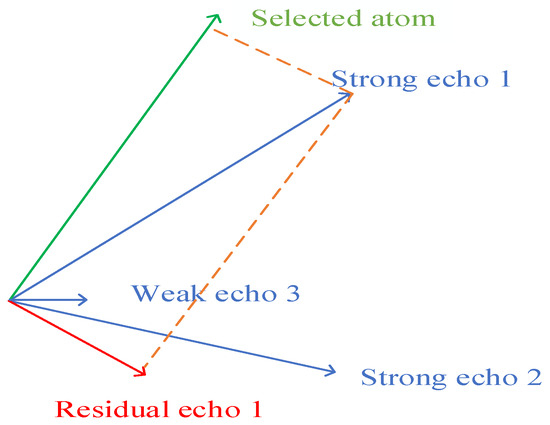
Step 3 of the OMP algorithm is essentially an orthogonal projection process. Due to the use of a discrete dictionary, there is always a mismatch between the true clutter components and the dictionary atoms, which leads to projection errors. As shown in Figure 6, when performing sparse representation for strong echo 1, the selected atom does not perfectly match strong echo 1, leaving residual components of echo 1 and thus forming projection errors. These projection errors have little impact on high-amplitude clutter atoms, which can therefore be accurately represented. In contrast, low-amplitude clutter atoms suffer from larger representation errors in the sparse representation.

Figure 6. Projection error.

Simulations are conducted to validate the above analysis, and the corresponding simulation parameters are summarized in Table 1.

Table 1. Simulation parameters.

Parameters	Doppler Frequency	Angle	Power
signal 1	0.1 Hz	23°	−126 dB
signal 2	−0.15 Hz	19°	−132 dB
signal 3	−0.2 Hz	17°	−137 dB

The simulation data are sparsely represented using the OMP algorithm, and the results are shown in Table 2. The simulation results indicate that the OMP algorithm fails to represent a weak signal.

Table 2. Sparse representation.

Parameters	Doppler Frequency	Angle	Power
coefficient 1	0.1 Hz	23°	−126.78 dB
coefficient 2	−0.15 Hz	19°	−132.34 dB
coefficient 3	0.11 Hz	23°	−137.21 dB

A threshold needs to be set to select the K atoms with the highest amplitudes from N clutter atoms. The selection is based on the criterion of maximizing the output SCNR. The threshold is adjusted iteratively, and the output SCNR is calculated using the K atoms exceeding the threshold. The threshold corresponding to the maximum SCNR is considered optimal.

$$\begin{array}{l}{\mathit{X}}_c={{\mathit{T}}_F}^H{\mathit{X}}_{ts},\\ \mathit{w}={{({\mathit{X}}_c{\mathit{X}}_c}^H)}^{-1}{{\mathit{T}}_F}^H\mathit{S},\\ SCN{R}_{out}={\displaystyle \frac{{\left|{\mathit{w}}^H{{\mathit{T}}_F}^H{\mathit{a}}_s\mathit{S}\right|}^2}{{{\mathit{w}}^H{\mathit{X}}_c{\mathit{X}}_c}^H\mathit{w}}},\end{array}$$

(19)

4. Measured Data Analysis

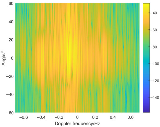
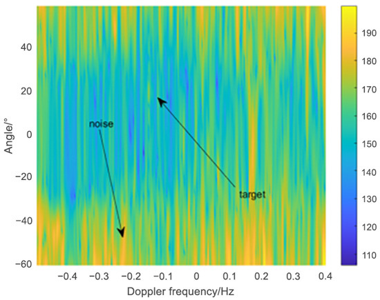
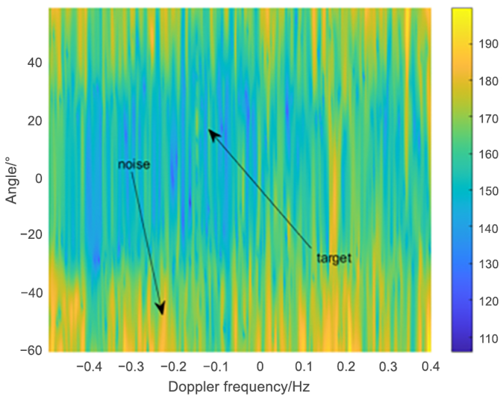
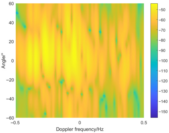
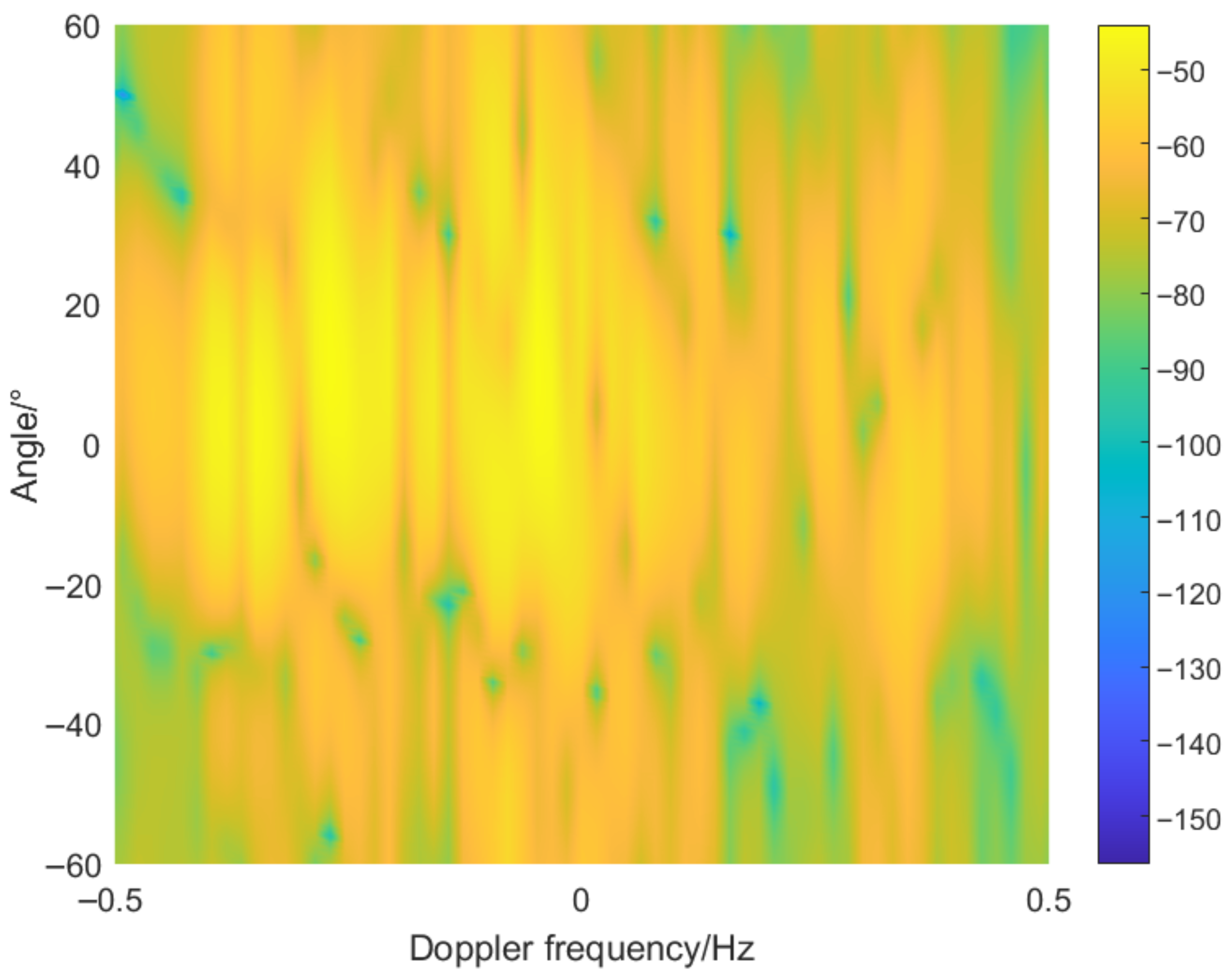
The 66th range cell was selected as the CUT, with the two neighboring range cells serving as guard cells, and the 69th range cell chosen as the training sample. Figure 7 shows the angle-Doppler map of the training sample. As can be seen from Figure 5 and Figure 7, the clutter distributions of the CUT and the training sample differ significantly.

Figure 7. Angle-Doppler map corresponding to the 69th range cell.

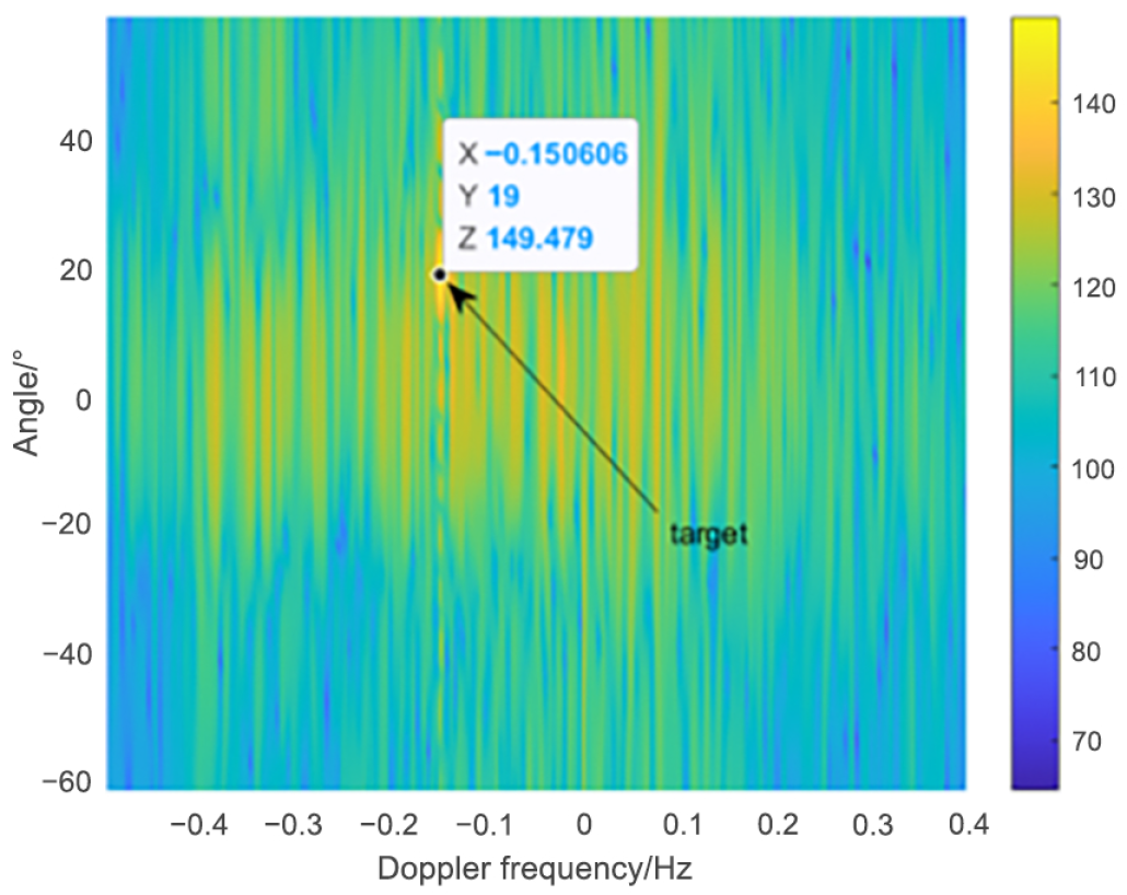
A target is added to the 66th range cell with an angle of 19° and a Doppler frequency of −0.15 Hz, and SCNR of −6 dB.

4.1. CPI Processing Results

The computer used in this experiment has 500 GB of memory. The full-dimensional SR-STAP algorithm based on sparse representation requires inverting the full-dimensional clutter covariance matrix, which exceeds the available memory. Therefore, this study first processes the complete CPI data, and then applies SR STAP using only 1/4 of the CPI data.

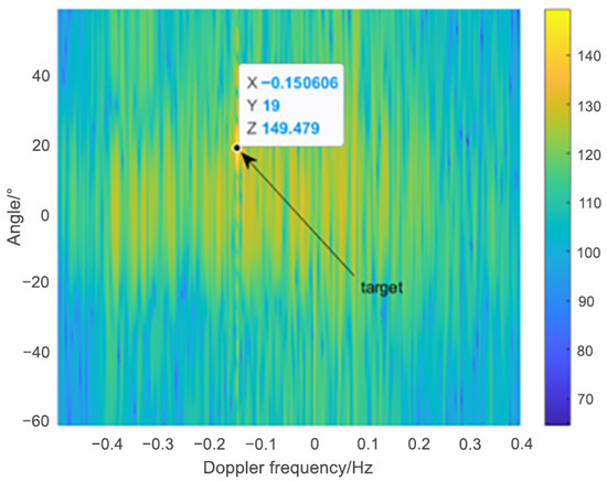
The processing results of the SCP algorithm are shown in Figure 8. It is evident that the SCP algorithm fails to detect the target. This is primarily because, with only a single training sample, the estimated clutter covariance matrix is inaccurate, resulting in a significant degradation of the algorithm’s performance and making target detection difficult.

Figure 8. Angle-Doppler map after SCP algorithm processing.

The processing results of the proposed algorithm are shown in Figure 9. It is evident that the algorithm achieves strong suppression of ionospheric clutter, maintaining good performance even with only a single highly non-uniform training sample. This is attributed to the proposed dimensionality-reduction matrix, which can effectively provide an accurate estimate of the clutter-plus-noise covariance matrix.

Figure 9. Angle-Doppler map after proposed method processing.

4.2. 1/4 CPI Processing Results

Both SR STAP and the calculation of SCNR loss require inverting the full-dimensional clutter covariance matrix, which exceeds the memory capacity of the computer used in this experiment. To facilitate performance comparison between the two algorithms, only 1/4 of the CPI data is used in this study.

Figure 10 shows the angle-Doppler map obtained using 1/4 CPI data at the CUT. It can be seen that reducing the accumulation time results in the Doppler resolution being reduced to one-fourth of its original value.

Figure 10. Angle-Doppler map of the 66th range cell using 1/4 CPI data.

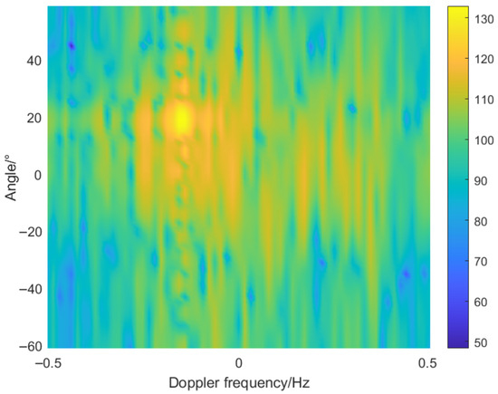
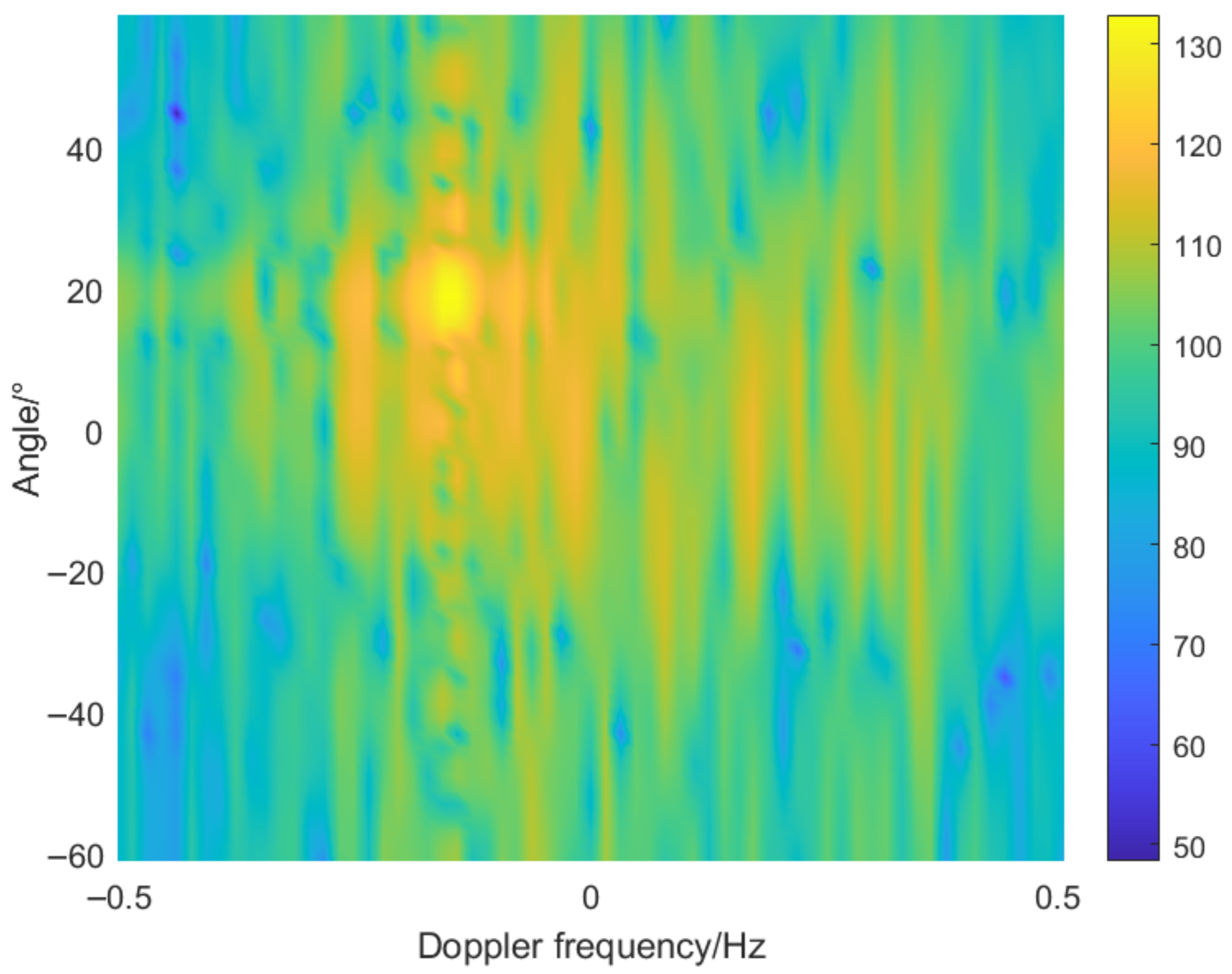
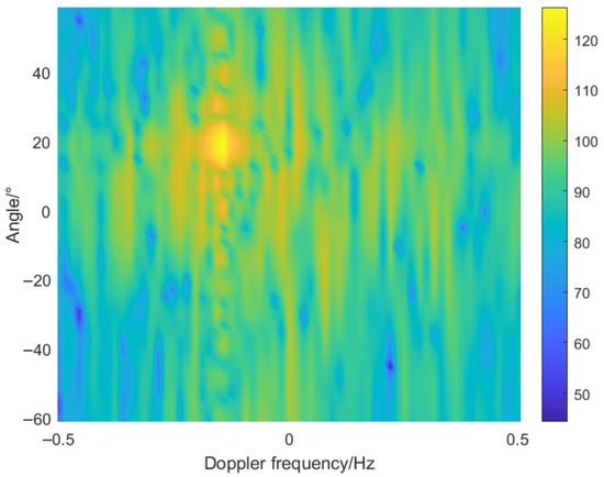
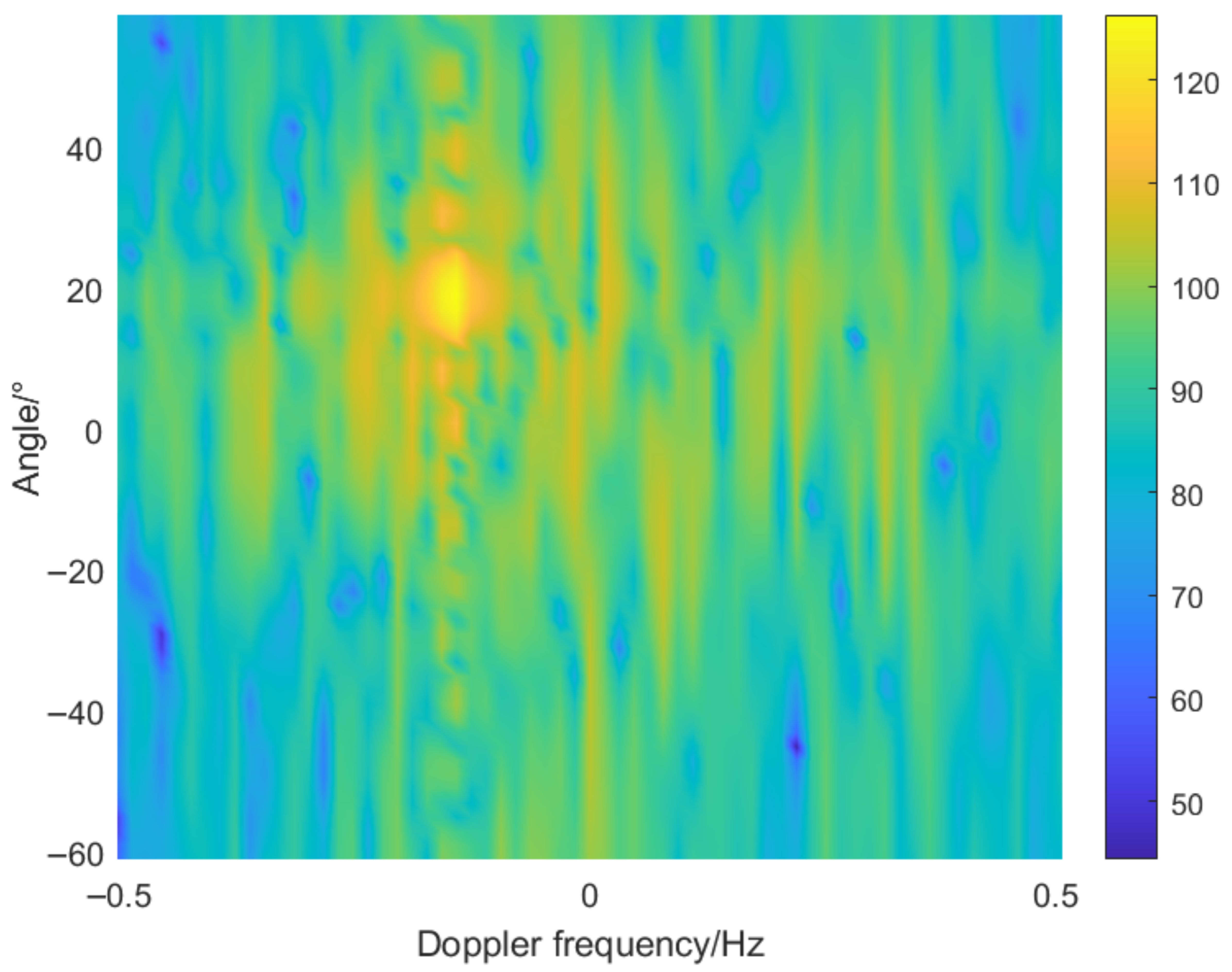
Figure 11 and Figure 12 show the processing results of the proposed algorithm and SR STAP, respectively. It can be observed that, although both methods are able to detect the target, SR STAP leaves significantly more residual ionospheric clutter.

Figure 11. Angle-Doppler map after SR STAP using 1/4 CPI data.

Figure 12. Angle-Doppler map after proposed method processing using 1/4 CPI data.

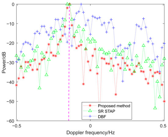
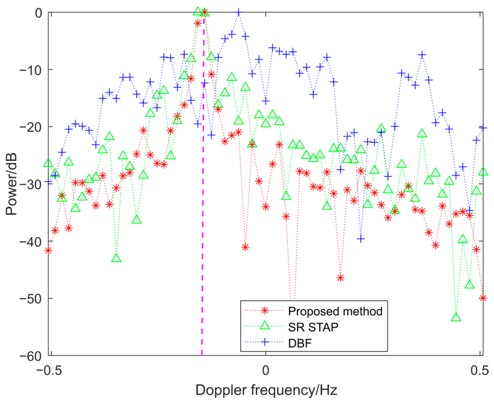
To examine the target’s Doppler frequency more closely, we plotted the Doppler profile along the target’s direction. As shown in Figure 13, the proposed method can accurately estimate the target’s Doppler frequency.

Figure 13. Doppler profiles of the 3 algorithms.

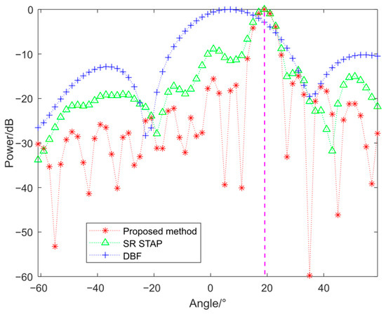
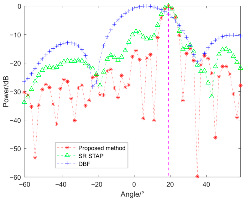
To examine the target’s angle information more closely, we plotted the angle profile along the target’s Doppler frequency. As shown in Figure 14, the digital beamforming (DBF) algorithm struggles to accurately determine the target’s angle, whereas the proposed algorithm can estimate it precisely.

Figure 14. Angle profiles of the 3 algorithms.

We use the SCNR loss formula to evaluate the performance of STAP.

$$\begin{array}{l}{\displaystyle \frac{SCN{R}_{out}}{SCN{R}_{opt}}}={\displaystyle \frac{{{({\mathit{T}}_F}^H\mathit{S})}^H{{({\mathit{T}}_F}^H{\mathit{R}}_c{\mathit{T}}_F)}^{-1}{({\mathit{T}}_F}^H\mathit{S})}{{{\mathit{S}}^H{\mathit{R}}_c}^{-1}\mathit{S}}},\\ {\mathit{R}}_c={\mathit{X}}_{ts}\ast {{\mathit{X}}_{ts}}^H,\end{array}$$

(20)

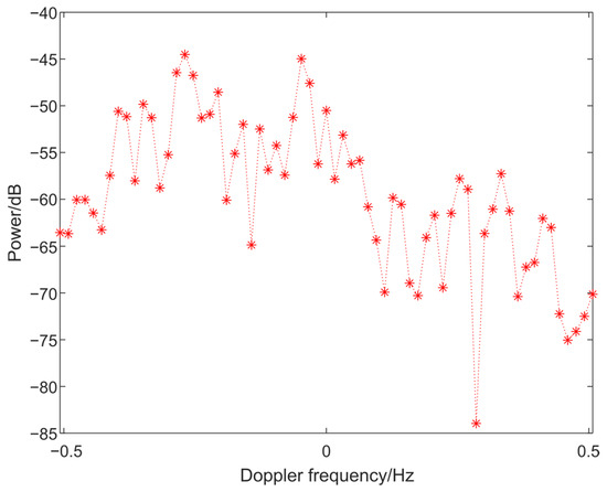
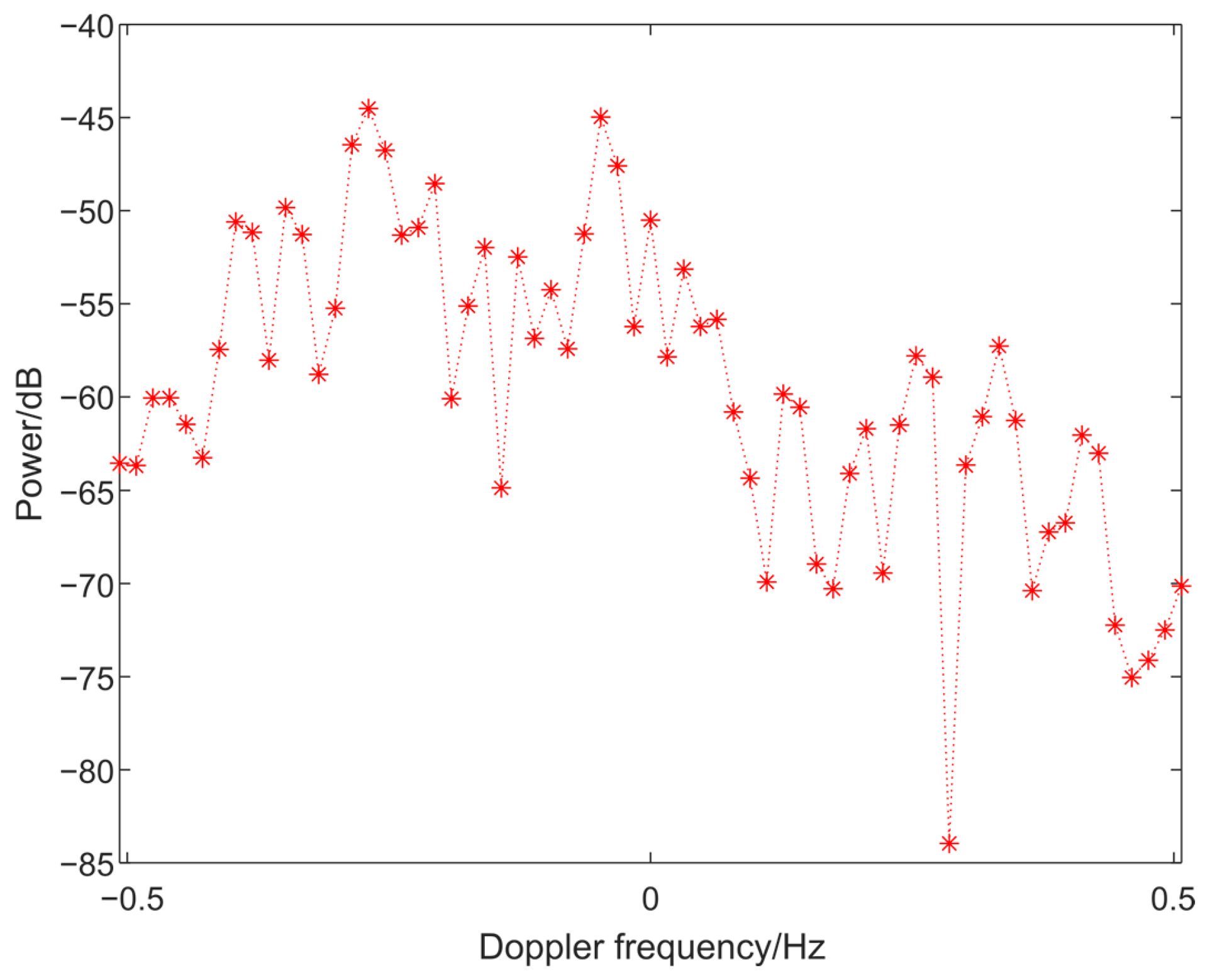
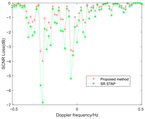
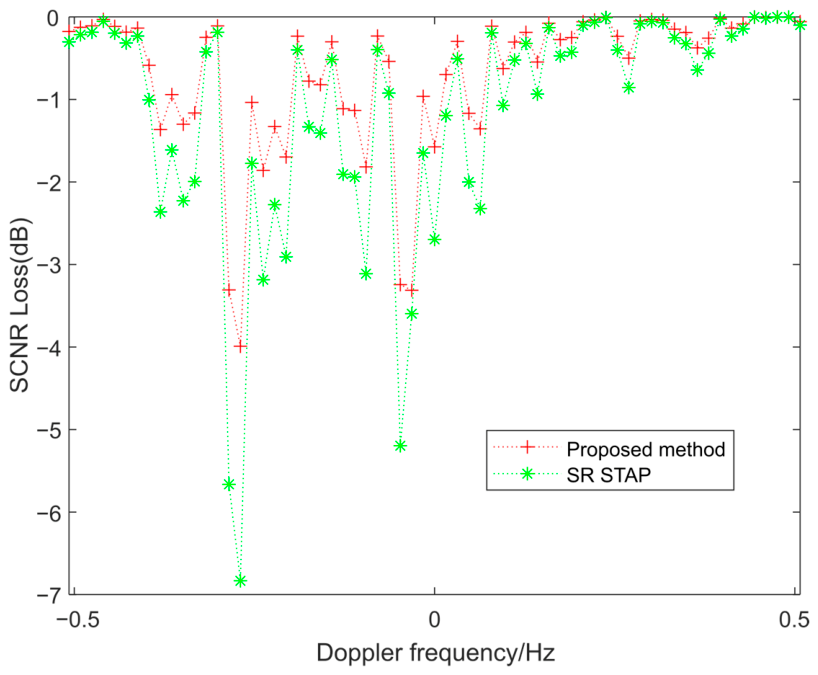
When evaluating STAP performance, the target angle is typically fixed while its Doppler frequency is varied to calculate the SCNR loss. In this study, 100 Monte Carlo trials were used to estimate the SCNR loss. As shown in Figure 15 and Figure 16, the proposed algorithm exhibits lower SCNR loss than SR STAP, indicating superior performance in suppressing ionospheric clutter.

Figure 15. Clutter power versus Doppler frequency in the target direction.

Figure 16. SCNR loss comparison with SR STAP.

To ensure practical applicability, it is necessary to compare the computational times of the two methods. As can be seen from Table 3, the proposed algorithm requires less computation time than SR STAP.

Table 3. Computation times of different methods.

Method	Computation Time
Proposed method	5 min
SR STAP	487 min

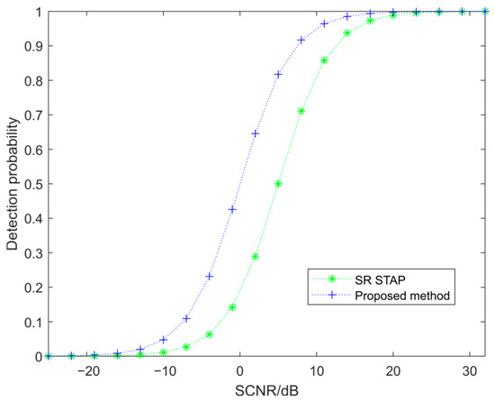
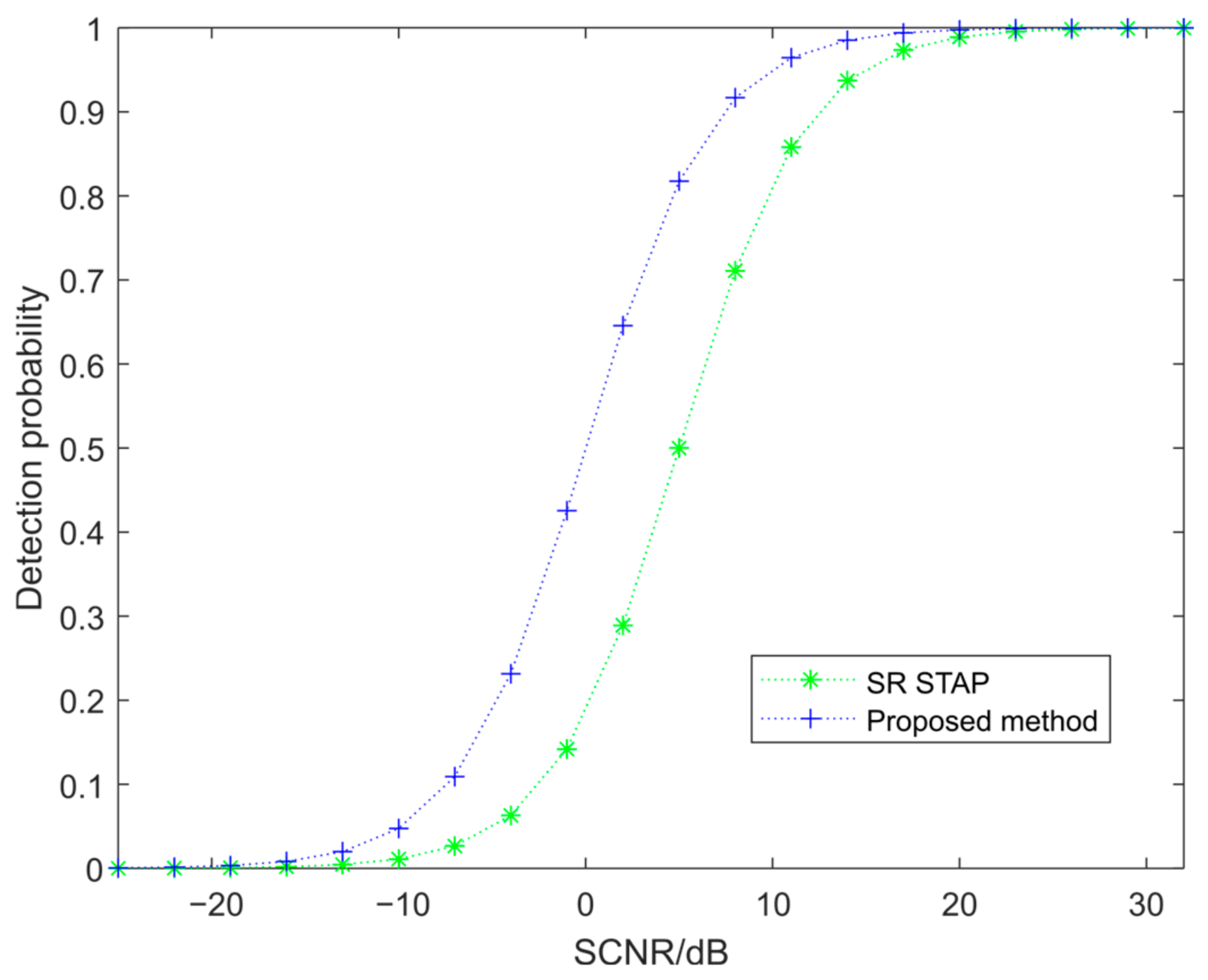
To illustrate the effect of the input SCNR on target detection performance, the constant false alarm rate (CFAR) detection probability is used as a reference metric. In the experiment, the false alarm rate was set to 10⁻⁴, and the total number of detection cells was 32. Figure 17 shows the CFAR detection probability under different input SCNRs. The results indicate that the target detection probability increases noticeably with SCNR. Compared to the full-dimensional STAP algorithm based on sparse representation, the proposed algorithm achieves a significantly higher detection probability, demonstrating its effectiveness in enhancing target detection performance after suppressing non-uniform ionospheric clutter.

Figure 17. CFAR detection probability versus input SCNR.

5. Conclusions

HFSWR often suffers from highly non-uniform striped ionospheric clutter, which significantly degrades sea-surface target detection performance. Full-dimension STAP algorithms based on sparse representation for reconstructing the clutter covariance matrix are computationally demanding and may exceed available memory resources, making them impractical for real-world applications. To address this issue, this paper proposes a reduced-dimension STAP algorithm based on sparse representation. Similar to Fourier transform, sparse representation is also constrained by angle and Doppler frequency resolution. In the proposed method, a dictionary is constructed by discretizing the Doppler frequency and spatial angle domains with appropriate resolution intervals, forming a grid of space-time atoms to represent clutter components. Both the training sample and the cell under test are then sparsely represented over this dictionary to extract consistent clutter components. Due to inevitable mismatches between the discretized dictionary atoms and the actual clutter characteristics, low-energy atoms are considered unreliable and are removed using a thresholding strategy. The remaining reliable atoms are used to construct a reduced-dimension projection matrix, enabling accurate estimation of the local clutter-plus-noise covariance matrix. Experimental results based on measured data demonstrate that the proposed method effectively suppresses striped ionospheric clutter and significantly improves sea-surface target detection performance. A main limitation of this work is the lack of higher angle resolution radar data, which restricts further validation of the proposed method in scenarios requiring fine angular discrimination. However, under the currently available resolution, the obtained results still demonstrate the effectiveness of the proposed method.

References

- Ji, Y.; Li, Z.; Wu, X.; Qu, R.; Wang, Y. First-Order Ocean Surface Echo Model for Shipborne HFSWR Based on Fusion Estimation of Antenna Displacement. IEEE Antennas Wirel. Propag. Lett. 2023, 22, 3082–3086. [Google Scholar] [CrossRef] [Scilit]
- Yi, C.; Ji, Z.; Kirubarajan, T.; Xie, J.; Hu, B. An Improved Oblique Projection Method for Sea Clutter Suppression in Shipborne HFSWR. IEEE Geosci. Remote Sens. Lett. 2016, 13, 1089–1093. [Google Scholar] [CrossRef] [Scilit]
- Wang, C.; Yu, H.; Zhang, L.; Li, G.; Wu, Q.M.J. Shipborne HFSWR Direction-Finding Method for Target Detection Based on Correction Matrix. IEEE Geosci. Remote Sens. Lett. 2025, 22, 3501005. [Google Scholar] [CrossRef] [Scilit]
- Brennan, L.E.; Reed, L.S. Theory of Adaptive Radar. IEEE Trans. Aerosp. Electron. Syst. 1973, AES-9, 237–252. [Google Scholar] [CrossRef] [Scilit]
- Guo, L.; Li, J.; Yang, Q.; Zhang, X.; Liang, C.; Bai, Y. A STAP clutter suppression algorithm based on sparse representation for small-array HFSWR. Remote Sens. Lett. 2022, 13, 611–620. [Google Scholar]
- Shi, J.; Xie, L.; Cheng, Z.; He, Z.; Zhang, W. Angle-Doppler Channel Selection Method for Reduced-Dimension STAP Based on Sequential Convex Programming. IEEE Commun. Lett. 2021, 25, 3080–3084. [Google Scholar] [CrossRef] [Scilit]
- Yong-Liang, W.; Jian-Wen, C.; Zheng, B.; Ying-Ning, P. Robust space-time adaptive processing for airborne radar in nonhomogeneous clutter environments. IEEE Trans. Aerosp. Electron. Syst. 2003, 39, 70–81. [Google Scholar] [CrossRef]
- Wang, H.; Lujing, C. On adaptive spatial-temporal processing for airborne surveillance radar systems. IEEE Trans. Aerosp. Electron. Syst. 1994, 30, 660–670. [Google Scholar] [CrossRef] [Scilit]
- Zhang, W.; An, R.; He, N.; He, Z.; Li, H. Reduced Dimension STAP Based on Sparse Recovery in Heterogeneous Clutter Environments. IEEE Trans. Aerosp. Electron. Syst. 2020, 56, 785–795. [Google Scholar] [CrossRef] [Scilit]
- Wang, Z.; Li, Y.; Wang, C.; Ouyang, D.; Huang, Y. A-OMP: An Adaptive OMP Algorithm for Underwater Acoustic OFDM Channel Estimation. IEEE Wirel. Commun. Lett. 2021, 10, 1761–1765. [Google Scholar] [CrossRef] [Scilit]
- Xie, K.; He, Z.; Cichocki, A. Convergence Analysis of the FOCUSS Algorithm. IEEE Trans. Neural Netw. Learn. Syst. 2015, 26, 601–613. [Google Scholar] [CrossRef] [Scilit]
- Möderl, J.; Leitinger, E.; Fleury, B.H. General Pruning Criteria for Fast SBL. IEEE Signal Process. Lett. 2025, 32, 4374–4378. [Google Scholar] [CrossRef] [Scilit]
- Wang, X.; Aboutanios, E.; Amin, M.G. Reduced-Rank STAP for Slow-Moving Target Detection by Antenna-Pulse Selection. IEEE Signal Process. Lett. 2015, 22, 1156–1160. [Google Scholar] [CrossRef] [Scilit]
- Fa, R.; Lamare, R.C.d.; Wang, L. Reduced-Rank STAP Schemes for Airborne Radar Based on Switched Joint Interpolation, Decimation and Filtering Algorithm. IEEE Trans. Signal Process. 2010, 58, 4182–4194. [Google Scholar] [CrossRef] [Scilit]
- Xiaoqin, W.; Chongzhao, H. Direct data domain approach to space-time adaptive processing. J. Syst. Eng. Electron. 2006, 17, 59–64. [Google Scholar] [CrossRef] [Scilit]
- Liu, C.; Wang, T.; Zhang, S.; Ren, B. A Clutter Suppression Algorithm via Weighted l2- norm Penalty for Airborne Radar. IEEE Signal Process. Lett. 2022, 29, 1522–1525. [Google Scholar] [CrossRef] [Scilit]
- Xie, L.; He, Z.; Tong, J.; Zhang, W. A Recursive Angle-Doppler Channel Selection Method for Reduced-Dimension Space-Time Adaptive Processing. IEEE Trans. Aerosp. Electron. Syst. 2020, 56, 3985–4000. [Google Scholar] [CrossRef] [Scilit]
- Ji, Y.; Zhang, J.; Wang, Y.; Chang, G.; Sun, W. Performance analysis of target detection with compact HFSWR. In Proceedings of the 2016 CIE International Conference on Radar (RADAR), Guangzhou, China, 10–13 October 2016; pp. 1–4. [Google Scholar]
- Saleh, O.; Adve, R.S.; Riddolls, R.J. Fast fully adaptive processing: A multistage STAP approach. In Proceedings of the 2009 IEEE Radar Conference, Pasadena, CA, USA, 4–8 May 2009; pp. 1–6. [Google Scholar]
- Su, Y.; Wei, Y.; Xu, R.; Liu, Y. Ionospheric clutter suppression using Wavelet Oblique Projecting Filter. In Proceedings of the 2017 IEEE Radar Conference (RadarConf), Seattle, WA, USA, 8–12 May 2017; pp. 1552–1556. [Google Scholar]
- Zhong, J.; Yu, H.; Zhang, L.; Li, G.; Wu, Q.M.J. Shipborne HFSWR Sea Clutter Suppression Method Based on MultiDomain Information Synergy. IEEE Geosci. Remote Sens. Lett. 2025, 22, 3503805. [Google Scholar] [CrossRef] [Scilit]
- Chen, S.; Gill, E.W.; Huang, W. A High-Frequency Surface Wave Radar Ionospheric Clutter Model for Mixed-Path Propagation With the Second-Order Sea Scattering. IEEE Trans. Antennas Propag. 2016, 64, 5373–5381. [Google Scholar] [CrossRef] [Scilit]
- Sevgi, L. Stochastic modeling and simulation studies for the surface wave high frequency radars: Problems and challenges. In Proceedings of the 2003 Proceedings of the International Conference on Radar (IEEE Cat. No.03EX695), Adelaide, Australia, 3–5 September 2003; pp. 602–607. [Google Scholar]
- Beck, A.; Teboulle, M. A fast Iterative Shrinkage-Thresholding Algorithm with application to wavelet-based image deblurring. In Proceedings of the 2009 IEEE International Conference on Acoustics, Speech and Signal Processing, Taipei, Taiwan, 19–24 April 2009; pp. 693–696. [Google Scholar]
- Ahire, R.B.; Patil, V.S. Overview of satellite image resolution enhancement techniques. In Proceedings of the 2013 Tenth International Conference on Wireless and Optical Communications Networks (WOCN), Bhopal, India, 26–28 July 2013; pp. 1–4. [Google Scholar]
- Demirel, H.; Anbarjafari, G. Discrete Wavelet Transform-Based Satellite Image Resolution Enhancement. IEEE Trans. Geosci. Remote Sens. 2011, 49, 1997–2004. [Google Scholar] [CrossRef] [Scilit]
- Zeng, W.; Lu, X. A PDE approach to super-resolution with contrast enhancement. In Proceedings of the 2010 3rd International Congress on Image and Signal Processing, Yantai, China, 16–18 October 2010; pp. 600–604. [Google Scholar]
- Sahoo, S.K.; Makur, A. Signal Recovery from Random Measurements via Extended Orthogonal Matching Pursuit. IEEE Trans. Signal Process. 2015, 63, 2572–2581. [Google Scholar] [CrossRef] [Scilit]
Disclaimer/Publisher’s Note: The statements, opinions and data contained in all publications are solely those of the individual author(s) and contributor(s) and not of MDPI and/or the editor(s). MDPI and/or the editor(s) disclaim responsibility for any injury to people or property resulting from any ideas, methods, instructions or products referred to in the content. |
© 2026 by the authors. Licensee MDPI, Basel, Switzerland. This article is an open access article distributed under the terms and conditions of the Creative Commons Attribution (CC BY) license.