Time-Domain Hydroelastic Analysis of Floating Structures Under Nonlinear Shallow-Water Waves over Variable Bathymetry

Abstract

Photovoltaic systems deployed on large floating platforms in nearshore waters are strongly influenced by hydroelastic effects, nonlinear shallow-water waves, and variable bathymetry. This study develops a time-domain hydroelastic framework that couples the fully nonlinear non-hydrostatic wave model NHWAVE with a Rankine-source potential-flow solver and a discrete-module Cummins formulation. The wave model provides incident pressures and kinematics over uneven seabeds, while the potential-flow solver evaluates radiation and diffraction effects and transfers the resulting hydrodynamic coefficients into the time domain. Numerical simulations are carried out for a 600 m modular floating structure under regular waves over flat and sloped bathymetries with $tan\alpha =0.0133$, wave periods of 4–6 s, and wave heights of 0.3–1.0 m. The results show that bathymetric variation intensifies shoaling-induced excitation, modifies added-mass and damping distributions, increases the spatial non-uniformity of hydroelastic motions, and amplifies bending-moment RMS responses relative to the flat-bottom case. Additional comparisons between rigid-body and hydroelastic models show clear period-dependent redistribution of motions and bending demand. These results demonstrate that both local bathymetry and structural elasticity must be considered for the reliable analysis and design of nearshore floating photovoltaic systems and other large floating structures.

1. Introduction

Large floating structures, including offshore photovoltaic systems and other nearshore installations, have attracted increasing attention in coastal regions where conventional fixed foundations are impractical [1]. Their hydroelastic behavior—arising from the coupled interaction between wave-induced loading and structural deformation—is a key factor governing structural safety and serviceability.

Recent studies have addressed various aspects of this problem. Chen et al. established a numerical framework for the hydroelastic analysis of flexible floating structures subjected to unsteady external excitations, with emphasis on global motions and internal force transfer [2]. Shi et al. subsequently investigated the hydroelastic response of offshore floating photovoltaic systems in the frequency domain under wave loading [3], while Li et al. examined the hydroelastic behavior of floating bridges under spatially inhomogeneous wave conditions, highlighting the role of drift-force modelling [4]. Zhang et al. further developed a frequency-domain hydroelastic model for membrane-based offshore photovoltaic platforms in regular waves [5], and Shi et al. extended the analysis of offshore floating photovoltaic systems to combined wind–wave loading scenarios [6].

In parallel, Chen et al. extended the discrete-module finite-element method to interconnected large flexible floating structures [7], while Wang et al. provided a comprehensive review of recent numerical, experimental, and field-based approaches for floating-bridge analysis [8].

Despite these advances, many practical deployments are located in coastal environments where water depth varies markedly over relatively short spatial scales. This issue is particularly pronounced in the Yellow Sea and Bohai coastal regions of China, where extensive continental shelves, shoals, tidal flats, and estuarine bathymetric transitions lead to significant spatial variability in water depth [9,10,11]. Under such conditions, incident waves undergo pronounced shoaling, refraction, diffraction, and nonlinear transformation, resulting in spatially heterogeneous wave fields that can substantially influence the hydroelastic response of large floating structures.

Traditional hydrodynamic analyses rely primarily on potential-flow solvers based on linear or weakly nonlinear theory. These methods assume mild nonlinearity, uniform bathymetry, and weak vertical accelerations, making them accurate in deep water but increasingly unreliable in shallow water. In particular, free-surface Green’s function approaches require a flat seabed and therefore cannot represent the rapidly varying bathymetry typical of nearshore sites [12,13,14,15]. Boussinesq-type models extend the validity of linear theory to shallow water, but their assumed polynomial vertical velocity profiles and weak-dispersion formulations limit accuracy when nonlinear shoaling or steep bathymetric gradients occur [16,17,18]. Recent nonlinear wave–structure studies have improved the prediction of wave transformation in coastal environments, including nonlinear modelling for flexible floating structures, yet the incident-wave model and the hydroelastic response model are still commonly treated as separate components, or coupled under assumptions that remain only weakly nonlinear [19,20,21].

To overcome these limitations, fully nonlinear non-hydrostatic wave models such as NHWAVE have been adopted to resolve wave shoaling, dispersion, and depth-induced waveform transformation over complex bathymetry [22]. Compared with linear or weakly nonlinear formulations, these models provide more reliable incident-wave kinematics and pressure fields for shallow-water hydroelastic analysis, especially when the local response depends on spatially varying pressure and velocity inputs rather than on a uniform incoming wave assumption.

Despite this progress, an important capability is still missing in the existing literature. Current studies can model hydroelastic response in inhomogeneous seas, and other studies can model nonlinear wave transformation over complex bathymetry, but they generally cannot do both within one consistent time-domain framework for nearshore flexible floating structures. For large floating structures subjected to spatially varying and nonlinear wave fields, a reliable analysis requires (i) incident-wave kinematics and pressure distributions obtained from a fully nonlinear wave model and (ii) a radiation–diffraction model that remains valid over non-uniform seabeds before the results are transferred into a time-domain hydroelastic solver [8,23]. Existing coupled Boussinesq–hydroelastic methods partially address this need, but they still rely on flat-bottom Green’s functions or boundary-condition treatments that are not fully consistent with potential-flow decomposition [20]. As a result, existing studies cannot yet provide a fully nonlinear, variable-bathymetry, time-domain hydroelastic analysis that simultaneously resolves incident-wave transformation, radiation–diffraction effects, and elastic structural response in one workflow.

To address these challenges, we develop a coupled hydroelastic framework that integrates a fully nonlinear wave-evolution module with a Rankine-source potential-flow solver formulated for varying bathymetry. The wave module provides the incident pressure field and fluid normal velocities in the absence of the floating structure; these fields are used to evaluate the Froude–Krylov excitation forces and to prescribe the incident boundary condition for the diffraction problem. Radiation and diffraction effects, including added mass, radiation damping coefficients, and wave-excitation transfer functions, are solved in the frequency domain using a Rankine-source method that accommodates arbitrary seabed topography.

Following the discrete-module hydroelastic formulation of Wei et al. [24,25], the resulting hydrodynamic coefficients are transformed into the time domain and integrated into Cummins’ equation [26] to obtain the structural response. The formulation includes equivalent beam stiffness, mooring restoring forces, and time-domain convolution terms representing fluid memory effects. Wave-model validation is followed by a systematic set of simulations in which a 600 m modular floating structure is subjected to regular waves over both flat and sloped bathymetries. Under representative wave periods and heights within practical design ranges, the study quantifies how varying bathymetry and the associated nonlinear shoaling modify added mass, damping, motion RMS responses, and bending-moment distributions. In addition, rigid-body versus hydroelastic comparisons are carried out for sloped-bathymetry cases at fixed $H=0.5\mathrm{m}$ and $T=4$–$6\mathrm{s}$ to assess the role of structural elasticity in motion and bending-demand redistribution.

Against this background, the contribution of the present study is not simply the use of another hydroelastic solver; it is the closure of the specific gap identified above. Existing studies cannot simultaneously resolve fully nonlinear shallow-water wave transformation over variable bathymetry, variable-depth radiation–diffraction effects, and time-domain hydroelastic response of a large flexible floating structure within one consistent computational procedure. The principal contributions of this study are therefore threefold. First, a time-domain hydroelastic analysis framework is formulated by combining NHWAVE-based incident-wave prediction with a Rankine-source radiation–diffraction solver over variable bathymetry. Second, a consistent procedure is established to transfer NHWAVE-derived incident pressure and normal-velocity information onto the wetted body boundary for Froude–Krylov and diffraction-force evaluation. Third, the coupled framework is applied to a modular floating structure to quantify how varying bathymetry changes motions and bending moments under representative wave conditions, and to show more clearly where a rigid-body idealization becomes inadequate.

2. Methodology

A time-domain hydroelastic framework is established by coupling a fully nonlinear shallow-water wave model, a potential-flow radiation–diffraction solver, and Cummins’ equation of motion. The procedure separates incident-wave prediction from the subsequent hydrodynamic and structural analyses, so nonlinear wave transformation and hydroelastic response can be treated within one consistent workflow.

First, a three-dimensional fully nonlinear wave model is used to compute the incident wave field in the absence of the floating bodies. This step provides the time-dependent free-surface elevation, pressure, and fluid velocity fields used as incident-wave input for the later hydrodynamic analysis.

Second, the radiation problem is solved in the frequency domain with a Rankine-source boundary element method that accounts for variable bathymetry. This step yields the added-mass and radiation-damping coefficients, from which the retardation function in the time-domain formulation is obtained.

Third, the wave-exciting forces are evaluated. The Froude–Krylov force is obtained by integrating the incident pressure over the wetted surface. The diffraction problem is then solved in the frequency domain using body-surface normal velocities prescribed from the incident-wave solution while retaining the effect of variable water depth.

Finally, the hydroelastic equations of motion are solved in the time domain using Cummins’ formulation. The resulting simulations provide the wave-induced motions and internal loads.

The coupling between the nonlinear wave model and the potential-flow solver is strictly one-way: NHWAVE provides the incident pressure and velocity fields that drive the Froude–Krylov and diffraction problems, but no feedback from the structure’s motions or radiated waves is returned to the wave model. This one-way arrangement is justified because the floating structure occupies a small fraction of the overall wave domain and its dynamic response does not measurably alter the incident-wave characteristics under the conditions considered. Consequently, the wave field computed by NHWAVE is treated as an undisturbed incident field, and the radiation and diffraction effects are handled entirely within the potential-flow solver.

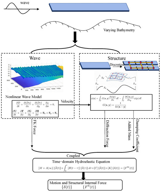
Figure 1 summarizes the information exchange among the nonlinear wave module, the Rankine-source hydrodynamic solver, and the time-domain motion solver. The wave model supplies the incident kinematics and pressures, and the resulting radiation and diffraction quantities are passed to the Cummins equation to compute the hydroelastic response.

Figure 1. Flow chart of the methodology.

3. Theory

This section presents the theoretical foundations of the proposed coupled hydroelastic framework. The governing formulation consists of three principal components. First, nonlinear wave propagation is resolved using the fully nonlinear wave model NHWAVE to provide the incident wave kinematics and pressure field over variable bathymetry. Second, a potential-flow model is employed to describe radiation and diffraction phenomena over the same variable-depth domain. Third, the hydroelastic response of the floating bodies is formulated in the time domain through the corresponding equations of motion. Together, these components establish a consistent framework for the analysis of wave–structure interactions in variable-depth environments.

3.1. Fully Nonlinear Wave Model

The governing equations of NHWAVE are the incompressible Navier–Stokes equations expressed in a well-balanced conservative form under a time-dependent free-surface and terrain-following $\sigma$-coordinate system, defined as [27]

$$\sigma ={\displaystyle \frac{z+h(x,y)}{D(x,y,t)}}$$

(1)

$$D(x,y,t)=h(x,y)+\eta (x,y,t),$$

(2)

where $(x,y)$ are the horizontal coordinates, z is the vertical coordinate measured upward from the still-water level, t is time, $h(x,y)$ denotes the still-water depth, and $\eta (x,y,t)$ is the free-surface elevation. This coordinate transformation essentially maps the physically varying vertical domain onto a uniformly transformed space in which $\sigma$ ranges from 0 to 1 [28].

Applying the $\sigma$-coordinate transformation, the well-balanced mass and momentum equations are given as follows:

$${\displaystyle \frac{\partial D}{\partial t}}+{\displaystyle \frac{\partial \left(Du\right)}{\partial x}}+{\displaystyle \frac{\partial \left(Dv\right)}{\partial y}}+{\displaystyle \frac{\partial \omega }{\partial \sigma }}=0,$$

(3)

$${\displaystyle \frac{\partial \mathbf{U}}{\partial t}}+{\displaystyle \frac{\partial \mathbf{F}}{\partial x}}+{\displaystyle \frac{\partial \mathbf{G}}{\partial y}}+{\displaystyle \frac{\partial \mathbf{H}}{\partial \sigma }}={\mathbf{S}}_h+{\mathbf{S}}_p+{\mathbf{S}}_s,$$

(4)

where $(u,v)$ are the horizontal velocity components, w is the physical vertical velocity component, and $\omega$ is the transformed vertical velocity in the $\sigma$ coordinate. The vector of conserved variables is $\mathbf{U}={(Du,Dv,Dw)}^{\mathrm{T}}$, and the fluxes are defined as

$$\mathbf{F}=\left[\begin{array}{c}D{u}^2+{\displaystyle \frac{1}{2}}g{D}^2\\ Duv\\ Duw\end{array}\right],\mathbf{G}=\left[\begin{array}{c}Duv\\ D{v}^2+{\displaystyle \frac{1}{2}}g{D}^2\\ Dvw\end{array}\right],\mathbf{H}=\left[\begin{array}{c}u\omega \\ v\omega \\ w\omega \end{array}\right].$$

(5)

The source terms consist of contributions from bed slope, pressure gradient, and turbulent stresses, expressed as

$${\mathbf{S}}_h=\left[\begin{array}{c}gD{\displaystyle \frac{\partial h}{\partial x}}\\ gD{\displaystyle \frac{\partial h}{\partial y}}\\ 0\end{array}\right],{\mathbf{S}}_p=\left[\begin{array}{c}-{\displaystyle \frac{D}{\rho }}\left({\displaystyle \frac{\partial p}{\partial x}}+{\displaystyle \frac{\partial p}{\partial \sigma }}{\displaystyle \frac{\partial \sigma }{\partial x}}\right)\\ -{\displaystyle \frac{D}{\rho }}\left({\displaystyle \frac{\partial p}{\partial y}}+{\displaystyle \frac{\partial p}{\partial \sigma }}{\displaystyle \frac{\partial \sigma }{\partial y}}\right)\\ -{\displaystyle \frac{1}{\rho }}{\displaystyle \frac{\partial p}{\partial \sigma }}\end{array}\right],{\mathbf{S}}_s=\left[\begin{array}{c}D{S}_{{\tau }_x}\\ D{S}_{{\tau }_y}\\ D{S}_{{\tau }_z}\end{array}\right],$$

(6)

where g is gravitational acceleration, $\rho$ is fluid density, and p is pressure. The terms $D{S}_{{\tau }_x},D{S}_{{\tau }_y},D{S}_{{\tau }_z}$ represent the turbulent stress terms. These terms are written in conservative form, as provided by [29].

Three modeling assumptions are adopted in the application of NHWAVE in the present study. First, the turbulent stress terms ${\mathbf{S}}_s$ are set to zero throughout all simulations. The wave conditions considered here are in the non-breaking propagation regime, so viscous dissipation and turbulent mixing play a negligible role compared with the dominant nonlinear shoaling dynamics, and no turbulence closure is required. Second, wave breaking is not activated in the model. The incident steepness values and local wave-height-to-depth ratios across all simulated cases remain below standard shallow-water breaking thresholds, and no breaking instability was observed in any run. Third, viscous effects in the fluid are entirely neglected; the flow is treated as inviscid throughout the wave-evolution computation.

After solving the above equations, the incident-wave pressure field $p_I$ and the velocity field ${\mathbf{v}}_I={(u,v,w)}^{\mathrm{T}}$ are available throughout the computational domain. These quantities are interpolated from the NHWAVE grid to the centroids of the wetted body panels on $S_B$. The incident pressure $p_I$ is integrated over $S_B$ to evaluate the Froude–Krylov contribution, while the projected incident normal velocity

$$v_n^I={\mathbf{v}}_I·\mathbf{n}$$

(7)

is imposed as the body-boundary input for the diffraction analysis, where $\mathbf{n}$ is the outward unit normal on the wetted body surface $S_B$. In this manner, the diffraction problem is driven by incident-wave kinematics that are consistent with the nonlinear shallow-water solution, while the radiation problem remains defined by the body motions themselves.

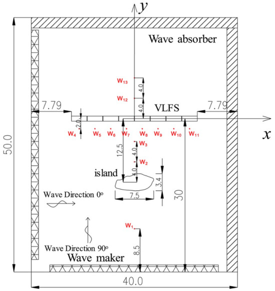
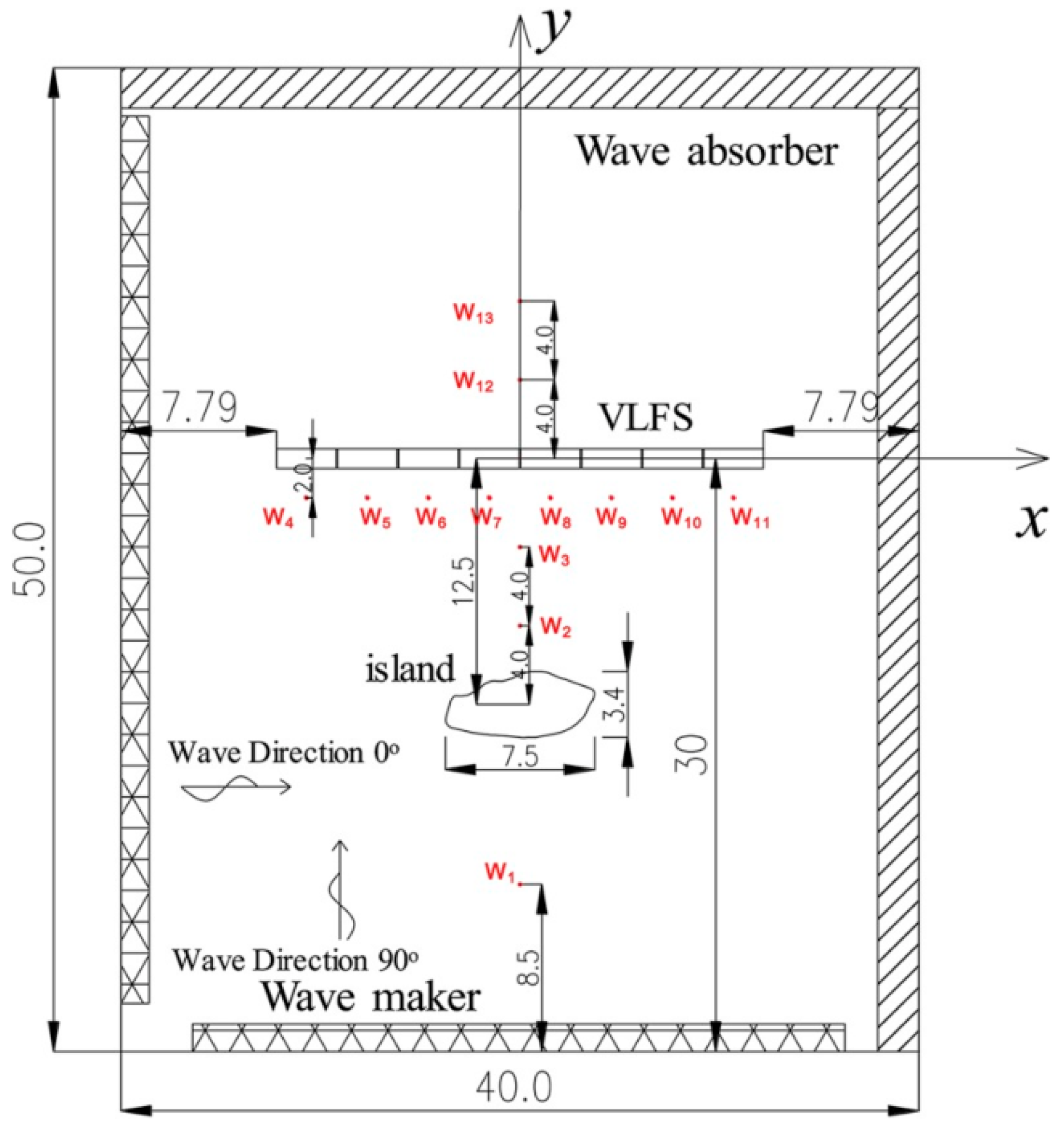
To verify the predictive capability of the nonlinear wave module before hydroelastic coupling, the present study adopts the island-topography validation case reported by Yang et al. [20]. The reference experiment was conducted in the deep-water wave basin of Shanghai Jiao Tong University with a varying-bottom configuration consisting of an island placed between the wavemaker and the floating-structure region together with a two-dimensional slope behind the structure. In the prototype-scale representation, the constant-depth offshore region has a water depth of $58.7\mathrm{m}$, and the wave field is monitored by thirteen probes, denoted $W1$–$W13$, distributed around the island and in its lee. The plan and longitudinal views of this setup are shown in Figure 2.

Figure 2. Plan view of the experimental configuration for the island-topography validation case, showing the wave basin, island, VLFS location, and thirteen wave gauges. Adapted from Yang et al. [20].

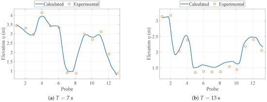
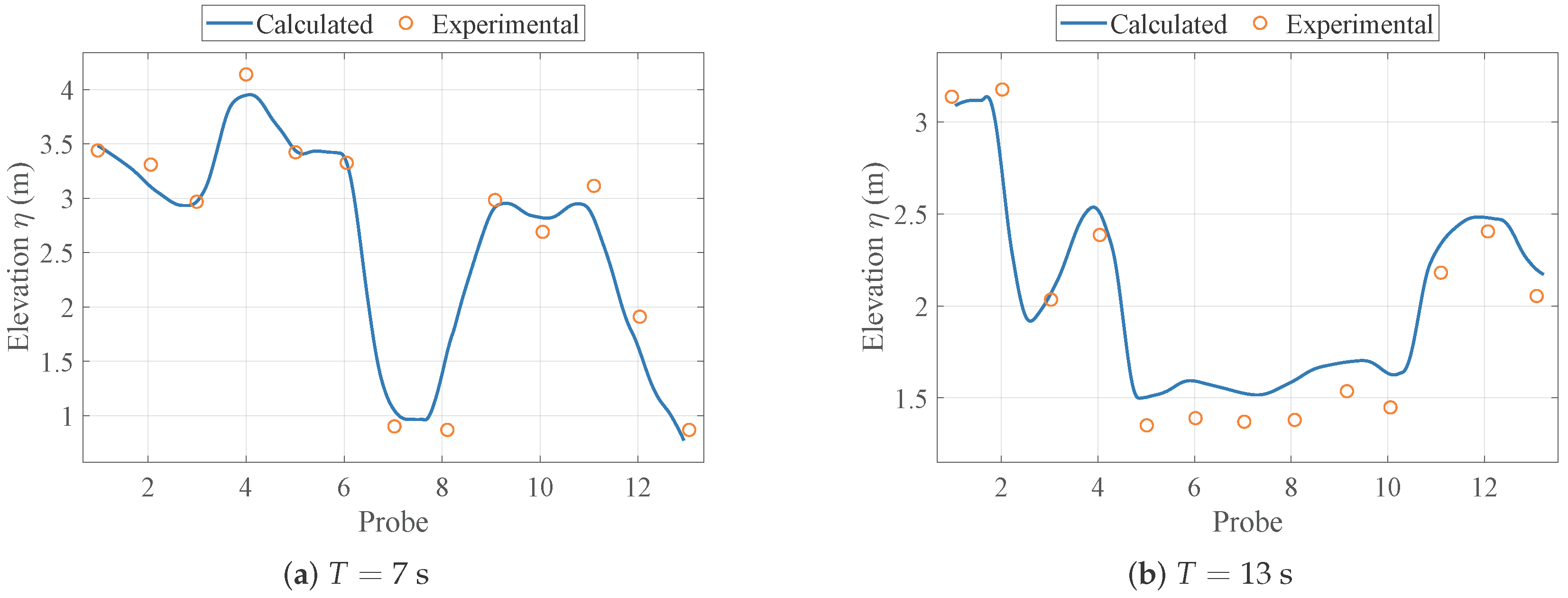
Following the reference setup, regular beam waves with incident wave height $H=3.0\mathrm{m}$ and wave direction ${90}^{\circ }$ are imposed for two representative periods, $T=7\mathrm{s}$ and $T=13\mathrm{s}$. Figure 3 compares the computed and measured wave heights at the thirteen gauge locations. The numerical results reproduce the main spatial trend reported by Yang et al. [20]: the wave field behind the island is strongly inhomogeneous, and the gauges located in the sheltered region exhibit substantially reduced wave heights relative to the gauges on both sides. The overall agreement for both wave periods confirms that the nonlinear wave module captures the combined effects of island-induced sheltering, diffraction, and bathymetry-controlled wave transformation with sufficient accuracy for the subsequent coupled hydroelastic simulations.

Figure 3. Validation of the nonlinear wave model against the thirteen-gauge island experiment of Yang et al. [20]. Comparisons are shown for regular beam waves with incident height $H=3.0\mathrm{m}$ at two wave periods.

3.2. Rankine Source Formulation over Spatially Varying Bathymetry

Unlike classical radiation–diffraction solvers that assume constant water depth, the present study considers a spatially varying seabed described by

$$z=-h(x,y),$$

(8)

which results in a non-planar bottom boundary. The radiation and diffraction problems are formulated within a potential-flow framework, which assumes an inviscid, irrotational fluid. Viscous effects and any free-surface turbulence generated by the incident waves are therefore excluded from this part of the analysis; these assumptions are consistent with standard boundary element practice and are justified for the radiation and diffraction conditions considered here.

For arbitrary bathymetry, analytical free-surface Green functions derived for uniform depth are no longer applicable, since they implicitly assume a horizontal seabed. Consequently, the bottom boundary condition must be enforced explicitly on the true geometric surface. The seabed boundary condition reads

$$\nabla \varphi ·{\mathbf{n}}_b=0\mathrm{on}{S}_d,$$

(9)

where $\varphi$ is the velocity potential and $S_d$ denotes the seabed boundary surface. The outward unit normal vector to the seabed is

$${\mathbf{n}}_b={\displaystyle \frac{(-h_x,-h_y,1)}{\sqrt{1+h_x^2+h_y^2}}}.$$

(10)

Here, $h_x=\partial h/\partial x$ and $h_y=\partial h/\partial y$ are the bottom-slope components in the x and y directions.

The presence of bathymetric gradients $h_x$ and $h_y$ introduces direct coupling between horizontal and vertical velocity components, which fundamentally modifies the structure of the boundary integral problem. Since no closed-form Green function exists for general depth variation, the problem is formulated using a Rankine source method.

Using the Rankine fundamental solution

$$G(\mathbf{x},\mathbf{y})={\displaystyle \frac{1}{4\pi |\mathbf{x}-\mathbf{y}|}},$$

(11)

Green’s second identity yields the boundary integral representation

$$\varphi \left(\mathbf{x}\right)={\int }_{\Gamma }G(\mathbf{x},\mathbf{y}){\displaystyle \frac{\partial \varphi \left(\mathbf{y}\right)}{\partial n}}d\Gamma -{\int }_{\Gamma }{\displaystyle \frac{\partial G(\mathbf{x},\mathbf{y})}{\partial n_{\mathbf{y}}}}\varphi \left(\mathbf{y}\right)d\Gamma ,$$

(12)

where $\Gamma$ consists of the free surface, the wetted body surface, the explicitly discretized bathymetric surface, and the artificial far-field boundary. In this expression, $\mathbf{x}$ is the field point, $\mathbf{y}$ is the source point, and $\partial /\partial n$ (or $\partial /\partial n_{\mathbf{y}}$) denotes differentiation along the outward boundary normal.

In contrast to constant-depth formulations, the seabed surface is treated as an independent boundary in the integral equation. The bathymetry is discretized using boundary panels that conform to the prescribed depth function $h(x,y)$. To accurately resolve strong geometric gradients, local mesh refinement is introduced in regions where $|\nabla h|$ is large, ensuring numerical stability and preserving solution accuracy; validation of the resulting Rankine-source implementation is provided in Appendix A.

The resulting collocated boundary integral equation leads to the frequency-dependent linear system

$$\mathbf{A}\left(\omega \right)\mathit{\varphi }=\mathbf{b},$$

(13)

in which bathymetric effects are incorporated directly through geometric enforcement of the non-planar seabed boundary condition. Here, $\mathbf{A}\left(\omega \right)$ is the frequency-dependent influence matrix, $\mathit{\varphi }$ is the vector of unknown boundary potential values, and $\mathbf{b}$ is the right-hand-side vector determined by the prescribed boundary conditions.

This formulation yields the frequency-dependent radiation coefficients $A\left(\omega \right)$ and $B\left(\omega \right)$.

3.3. Time-Domain Hydroelastic Analysis of Floating Body

Following the time-domain formulation proposed by Cummins [26], the motion of a floating elastic structure can be expressed as

$$\left[M+A(\infty )\right]\left\{\ddot{\delta }\left(t\right)\right\}+{\int }_0^t\left[H(t-\tau )\right]\left\{\dot{\delta }\left(\tau \right)\right\}d\tau +\left[C\right]\left\{\dot{\delta }\left(t\right)\right\}+\left[K\right]\left\{\delta \left(t\right)\right\}=\left\{F^{\mathrm{W}}\left(t\right)\right\}.$$

(14)

Here, $\left\{\delta \right(t\left)\right\}$ denotes the generalized displacement vector of the floating body, including both rigid-body motions and elastic deformations, and the superposed dot represents differentiation with respect to time. The matrix $\left[M\right]$ is the structural mass matrix of the discretized body, while $\left[A\right(\infty \left)\right]$ represents the added-mass matrix evaluated at infinite frequency. The convolution term accounts for radiation memory effects, in which $\left[H\right(t\left)\right]$ is the retardation function. The matrix $\left[C\right]$ denotes external linear damping, and $\left[K\right]$ is the global stiffness matrix incorporating both structural elastic stiffness and mooring restoring stiffness. In the convolution integral, $\tau$ is the retardation-time dummy variable.

The retardation function is obtained from the frequency-domain radiation damping matrix $\left[B\right(\omega \left)\right]$ through the inverse cosine transform

$$\left[H\left(t\right)\right]={\displaystyle \frac{2}{\pi }}{\int }_0^{+\infty }\left[B\left(\omega \right)\right]cos\left(\omega t\right)d\omega .$$

(15)

Here, $\omega$ denotes angular frequency.

The total wave-exciting force $\left\{F^{\mathrm{W}}\left(t\right)\right\}$ consists of incident-wave and diffraction-wave contributions,

$$\left\{F^{\mathrm{W}}\left(t\right)\right\}=\left\{F^{\mathrm{I}}\left(t\right)\right\}+\left\{F^{\mathrm{D}}\left(t\right)\right\},$$

(16)

with

$$\left\{F^{\mathrm{I}}\left(t\right)\right\}=-{\oint }_{S_B}{p}_I\mathbf{n}\mathrm{d}S,$$

(17)

$$\left\{F^{\mathrm{D}}\left(t\right)\right\}=-{\oint }_{S_B}{p}_D\mathbf{n}\mathrm{d}S,$$

(18)

where $S_B$ denotes the wetted surface of the body, $\mathbf{n}$ is the outward unit normal vector, and $p_I$ and $p_D$ are the hydrodynamic pressures induced by the incident and diffraction potentials, respectively. The term $\mathrm{d}S$ denotes the differential surface element on $S_B$.

In the present study, this time-domain hydroelastic formulation is implemented using the discrete module method [24,25]. The continuous floating structure is discretized along its longitudinal direction into a series of rigid modules. Adjacent modules are interconnected by equivalent elastic beam elements that reproduce the global flexural rigidity of the original structure. Each module undergoes rigid-body motion, while structural elasticity is represented through the relative displacements and rotations between neighboring modules. The equivalent beam stiffness is assigned such that the assembled global stiffness matrix preserves the overall bending characteristics of the continuous body. Transverse deformation within each module is neglected, and the structure is assumed rigid in the lateral direction, so that the dominant hydroelastic response is governed by longitudinal bending modes.

Hydrodynamic quantities, including added mass, radiation damping, and wave-exciting forces, are evaluated on a module-by-module basis. This dual discretization strategy, combining structural segmentation with local hydrodynamic evaluation, enables efficient integration of the nonlinear wave field over variable bathymetry with the time-domain hydroelastic response of large floating structures. The resulting system is subsequently integrated in the time domain to obtain the hydroelastic motions.

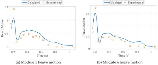
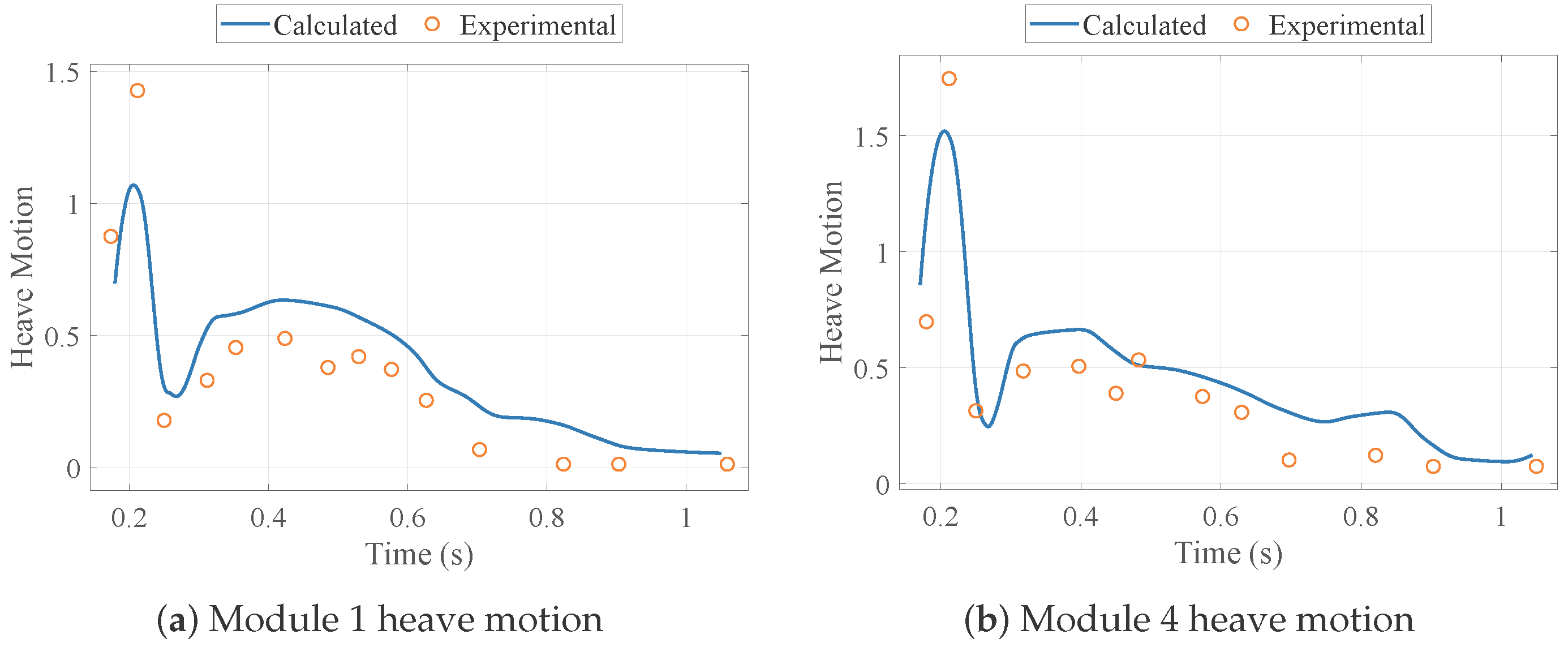
To further verify the time-domain hydroelastic solver against experimental data, the same island-topography setup introduced in Figure 2 is considered here using the measurements reported by Yang et al. [20]. Representative comparisons of the heave-motion time histories for Module 1 and Module 4 are presented in Figure 4. The numerical predictions reproduce the main transient characteristics of the measured responses, including the initial peak, the subsequent decay trend, and the relative difference between the upstream and downstream modules. Although some discrepancy remains in the peak magnitude and in parts of the later-stage response, the overall agreement indicates that the present Cummins-based discrete-module formulation can provide a reasonable time-domain prediction of the hydroelastic motion under experimentally observed inhomogeneous-wave conditions.

Figure 4. Validation of the time-domain hydroelastic response against the experimental data of Yang et al. [20] for the island-topography test case shown in Figure 2.

4. Results and Discussion

4.1. Numerical Configuration

The numerical investigations were performed using the coupled modelling framework introduced in the preceding sections. Nonlinear wave propagation was simulated with NHWAVE [22] on a quasi-two-dimensional computational domain discretized by 3500 cells in the streamwise direction, 10 cells in the transverse direction, and 5 vertical layers, with uniform horizontal spacing of $0.20\mathrm{m}$. The choice of 5 vertical layers follows the practical NHWAVE resolution strategy adopted by Ma et al. [22] and was retained here because preliminary vertical-resolution checks showed that further refinement produced negligible changes in the computed incident-wave elevations and pressures. Each simulation was carried out for $1000\mathrm{s}$, with an initial time step of $0.10\mathrm{s}$, adaptive bounds of $0.001$–$0.50\mathrm{s}$, a Courant limit of 0.5, and output written every $0.20\mathrm{s}$. The flow model was configured with second-order spatial and temporal discretization. At the upstream boundary, regular linear waves were prescribed, while the remaining boundaries followed the corresponding standard non-inflow settings. Frequency-domain radiation–diffraction problems were solved using a Rankine-source boundary element method, and the resulting hydrodynamic coefficients were subsequently incorporated into a discrete-module Cummins formulation. Fully coupled time-domain hydroelastic responses were then evaluated using the Newmark-$\beta$ time integration scheme.

To examine how varying bathymetry influences the response under different regular-wave conditions, a series of cases with different periods and heights was considered. The wave periods were selected as $T=4,5,6\mathrm{s}$, covering short- to intermediate-wave conditions that are representative of moderate coastal wind-sea environments and commonly adopted practical wave ranges for nearshore wave-transformation and wave-structure analyses [30,31,32,33]. For each period, three representative wave heights were prescribed, namely $H=0.3,0.5,1.0\mathrm{m}$, so that the test matrix spans mild to moderately energetic conditions while remaining suitable for systematic comparison of shoaling-induced nonlinearity and hydroelastic response redistribution. Both flat-bottom and sloped-bottom bathymetries were examined to quantify the influence of depth variation on the hydrodynamic and hydroelastic responses across these wave conditions. The complete set of numerical cases is summarized in Table 1.

Table 1. Summary of numerical case conditions.

Category	Case Type	Parameters
Bathymetry	Flat bottom/Sloped bottom	–
Regular waves	Wave period	$T=4,5,6\mathrm{s}$
	Wave height	$H=0.3,0.5,1.0\mathrm{m}$

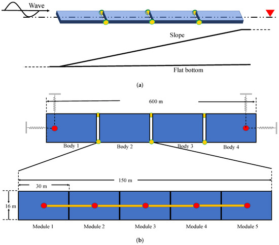
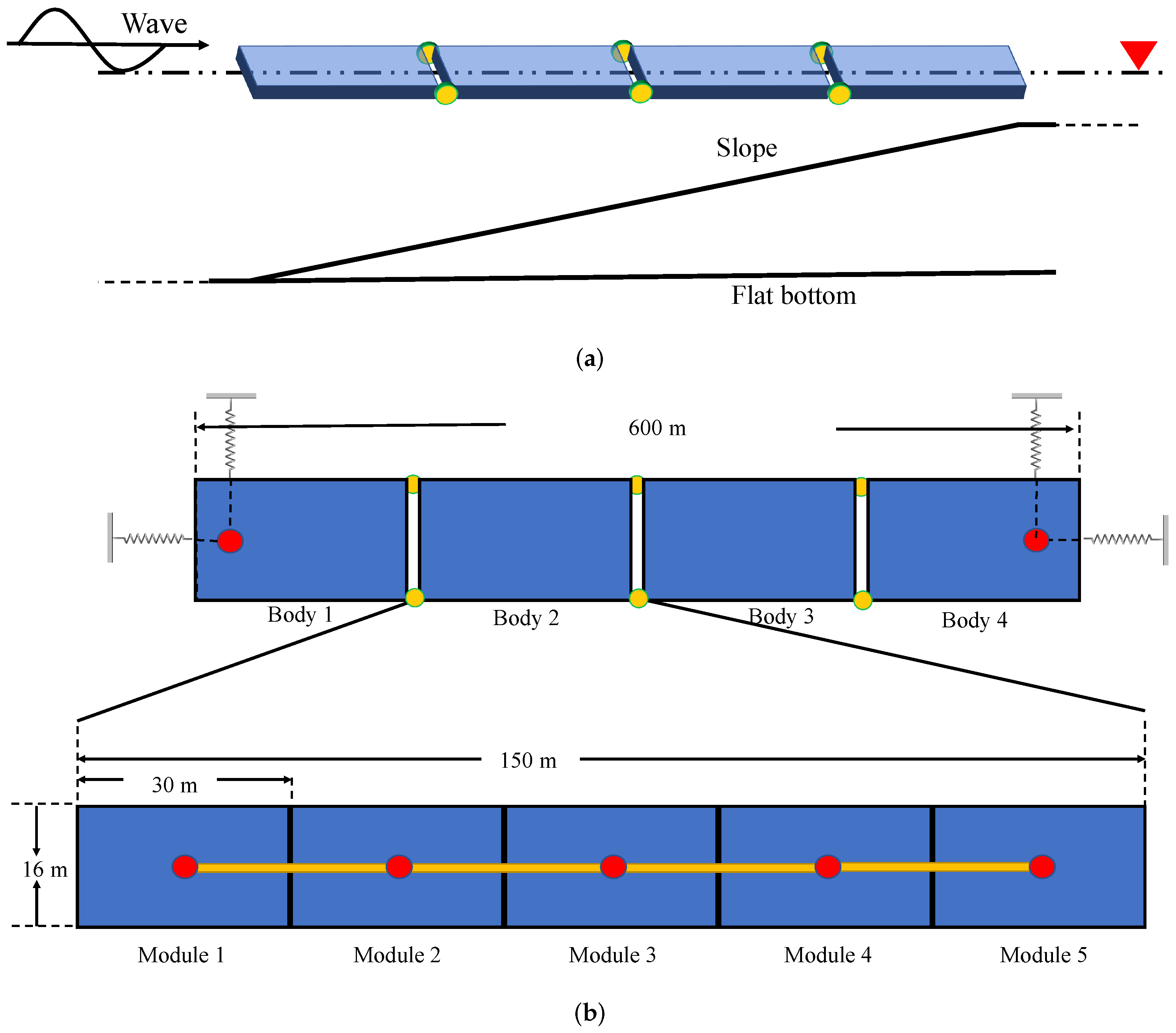
Two representative seabed configurations were adopted: a constant-depth flat bottom serving as the reference case and a linearly sloping bathymetry representing variable-depth conditions. These two bathymetries are shown together with the floating-body arrangement in Figure 5a, and their geometric definitions are summarized in Table 2.

Figure 5. Arrangement and discretization of the floating body over the variable seabed. (a) Side-view arrangement of the modular floating body for the flat-bottom and sloped-bottom bathymetries. (b) Discretization of each module.

Table 2. Definition of seabed configurations considered in the numerical study. The sloped bathymetry enables systematic assessment of depth-induced hydrodynamic variability.

Case	Total Length (m)	Slope Length (m)	${\mathit{h}}_{max}$ (m)	${\mathit{h}}_{min}$ (m)	Slope ($tan\mathit{\alpha }$)
Flat Bottom	700	–	10	10	0.0000
Slope	700	600	10	2	0.0133

The principal geometric characteristics and structural properties of the floating structure are summarized in Table 3. These parameters were selected to represent a large, shallow-draft modular floating structure operating in regions with pronounced depth variation. The corresponding two-node bending natural frequency is $0.162\mathrm{Hz}$, which corresponds to a natural period of approximately $6.17\mathrm{s}$.

Table 3. Principal geometric and structural properties of each module of the floating structure used in the hydroelastic simulations.

Parameter	Value
Total length, L (m)	150
Breadth, B (m)	16
Depth, D (m)	2
Draft, $T_d$ (m)	1
Vertical left of gravity above baseline, $KG$ (m)	0.5
Displacement, M (Mkg)	2.46
Vertical bending stiffness, $E{I}_y$ (MN·m2)	16,800
Horizontal bending stiffness, $E{I}_z$ (MN·m2)	840,000
Torsional stiffness, $G{I}_t$ (MN·m2)	2968

Figure 5 presents the arrangement of the floating body over the two adopted bathymetries together with the discretization strategy. The structure has a total length of $600\mathrm{m}$ and consists of four interconnected modules linked by hinges, each with a length of $150\mathrm{m}$ (Figure 5a). The bow of the floating body is positioned at the onset of the bathymetric transition, located $50\mathrm{m}$ from the wave-generation boundary.

A discrete-module approach was employed to analyse the hydroelastic response. Each $150\mathrm{m}$ module was further subdivided into five rigid sub-modules of $30\mathrm{m}$ length, as shown in Figure 5b. This discretization strategy allows accurate representation of the global bending deformation of the floating body under nonlinear shallow-water wave excitation while maintaining computational efficiency.

To compute the motion response of the floating body, prescribed linear stiffness and damping characteristics were introduced into the six-degree-of-freedom system. These restraints were imposed at two locations positioned $15\mathrm{m}$ inboard from the bow and stern of the modular structure. The adopted coefficients follow the linearized restraint treatment used in the present discrete-module hydroelastic model and are taken from the parameter setting reported in [34]. In this study, they are used to represent equivalent low-frequency restoring and damping effects of the station-keeping system in a simplified manner, rather than to model a specific detailed mooring layout. In the translational degrees of freedom, the surge and sway stiffnesses were both set to $200,000\mathrm{N}/\mathrm{m}$ ($200\mathrm{kN}/\mathrm{m}$), whereas no additional linear stiffness was applied in heave because the restoring force in that direction was primarily provided by hydrostatic pressure. In the rotational degrees of freedom, the hydrostatic stiffnesses were specified as $1.0\times {10}^5\mathrm{N}·\mathrm{m}/\mathrm{rad}$ in pitch, $1.0\times {10}^8\mathrm{N}·\mathrm{m}/\mathrm{rad}$ in roll, and $1.0\times {10}^6\mathrm{N}·\mathrm{m}/\mathrm{rad}$ in yaw. The damping coefficients were taken as $100,000\mathrm{N}·\mathrm{s}/\mathrm{m}$ in surge, $20,000\mathrm{N}·\mathrm{s}/\mathrm{m}$ in sway, and $1.0\times {10}^6\mathrm{N}·\mathrm{m}·\mathrm{s}/\mathrm{rad}$ in yaw.

For the wave-evolution simulations, four observation points were defined along the propagation direction at $x=50$, 250, 450, and $650\mathrm{m}$ measured from the wave-generation boundary, corresponding to Points A–D, respectively. For the sloped-bathymetry case, these locations span the depth transition from $10.0\mathrm{m}$ at Point A to $2.0\mathrm{m}$ at Point D, with intermediate depths of approximately $7.33\mathrm{m}$ and $4.67\mathrm{m}$ at Points B and C. This placement allows the progressive effects of shoaling to be tracked from the offshore region to the shallow end of the domain.

The numerical campaign was organized into two complementary components. The first component comprised wave-evolution simulations (Section 4.2), in which regular waves were propagated over the prescribed bathymetries to quantify wave shoaling and nonlinear waveform evolution. The second component comprised hydroelastic response simulations (Section 4.3 and Section 4.4), including comparisons of frequency-domain hydrodynamic coefficients under different bathymetric conditions, time-domain predictions of wave excitation, structural motions, and internal loads under regular-wave environments, and rigid-body versus hydroelastic comparisons to assess the role of structural elasticity.

4.2. Wave Evolution over Variable Bathymetry

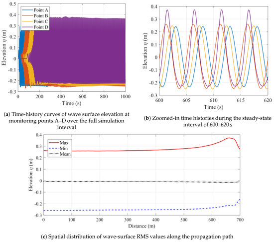
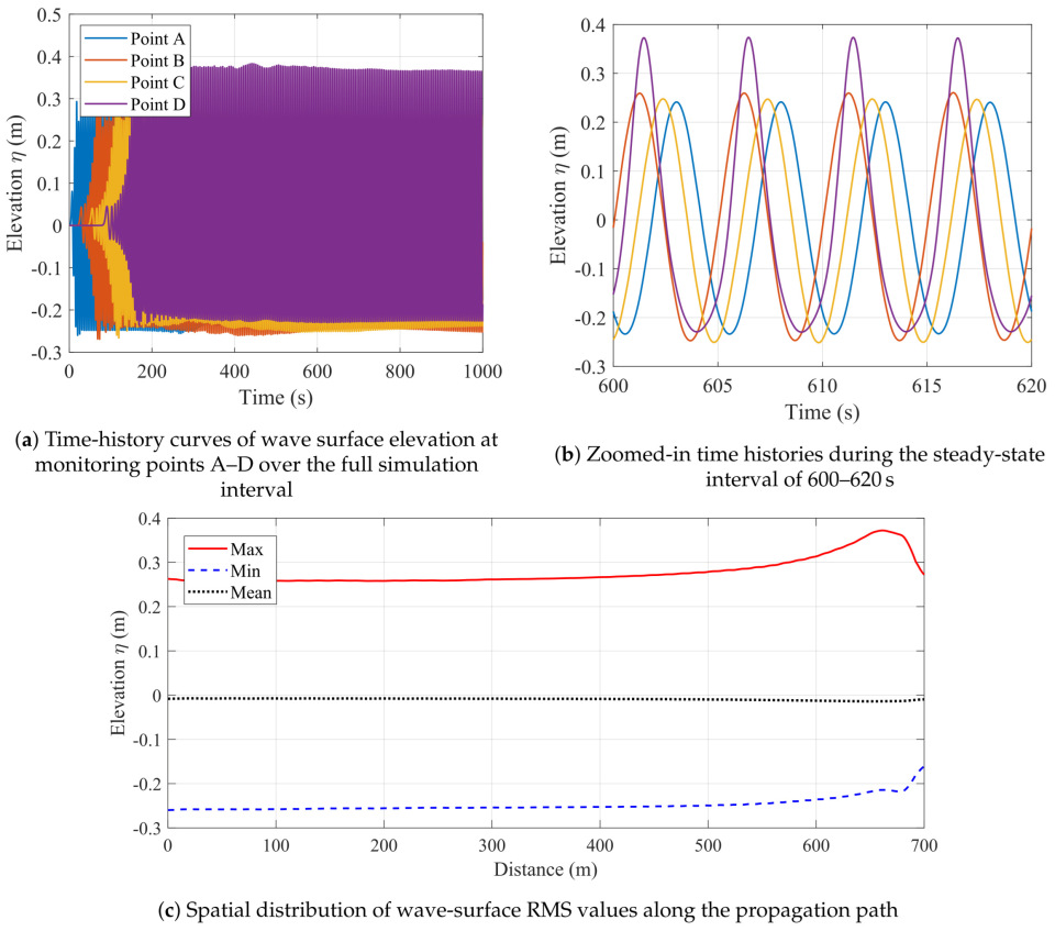
The NHWAVE simulations successfully reproduce the canonical shoaling process and the associated nonlinear deformation of regular waves propagating from deep to shallow water. Figure 6 presents representative results for a linear slope configuration, where time histories are recorded at the four observation points (Points A–D) defined in Section 4.1.

Figure 6. Wave evolution for the representative case ($T=5\mathrm{s}$): (a) Time histories of wave elevation at monitoring points A–D over the full simulation interval; (b) Zoomed-in time histories during the steady-state interval of 600–$620\mathrm{s}$; and (c) Spatial wave RMS distributions along the sloping seabed, including maximum and minimum RMS values and mean water level, illustrating wave shoaling and nonlinear waveform deformation.

For the representative incident condition ($H=0.5$ m, $T=5$ s), the time histories in Figure 6a,b show that the wave amplitudes at Points A and B are very similar, Point C is only slightly smaller, and Point D is markedly larger than the other three locations. The shallowest point exhibits the strongest crest growth, with the crest elevation reaching approximately $1.5$–$1.6$ times the incident wave height. The spatial RMS distribution in Figure 6c shows the same pattern: only minor variation is observed over the upstream part of the domain, followed by a clear increase toward the shallow end.

This curve pattern is consistent with the local depth conditions along the slope. At Points A–C, the water remains sufficiently deep that depth-induced shoaling is still weak, so the wave amplitude changes very little. By contrast, Point D is located in much shallower water, where the conservation of wave energy flux over decreasing depth leads to strong shoaling and therefore pronounced amplitude amplification.

Figure 6b further shows that the waveform becomes increasingly asymmetric as the wave propagates shoreward: the crest becomes steeper and narrower, whereas the trough becomes flatter and broader. This deformation is most evident near Point D during the steady-state interval (600–620 s). The reason is that nonlinear shallow-water effects intensify as the relative depth decreases, causing the wave profile to evolve toward a more Stokes-like shape. Although the crest is strongly amplified, the mean water level changes only slightly, because the sharper crest occupies a relatively short portion of each wave cycle and is partly offset by the broadened trough.

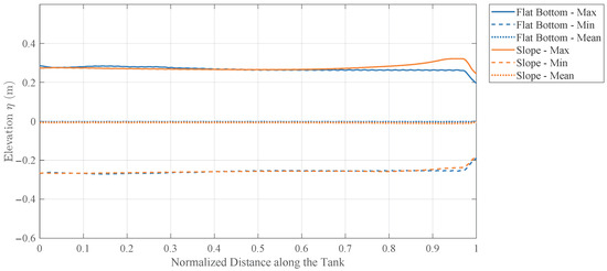
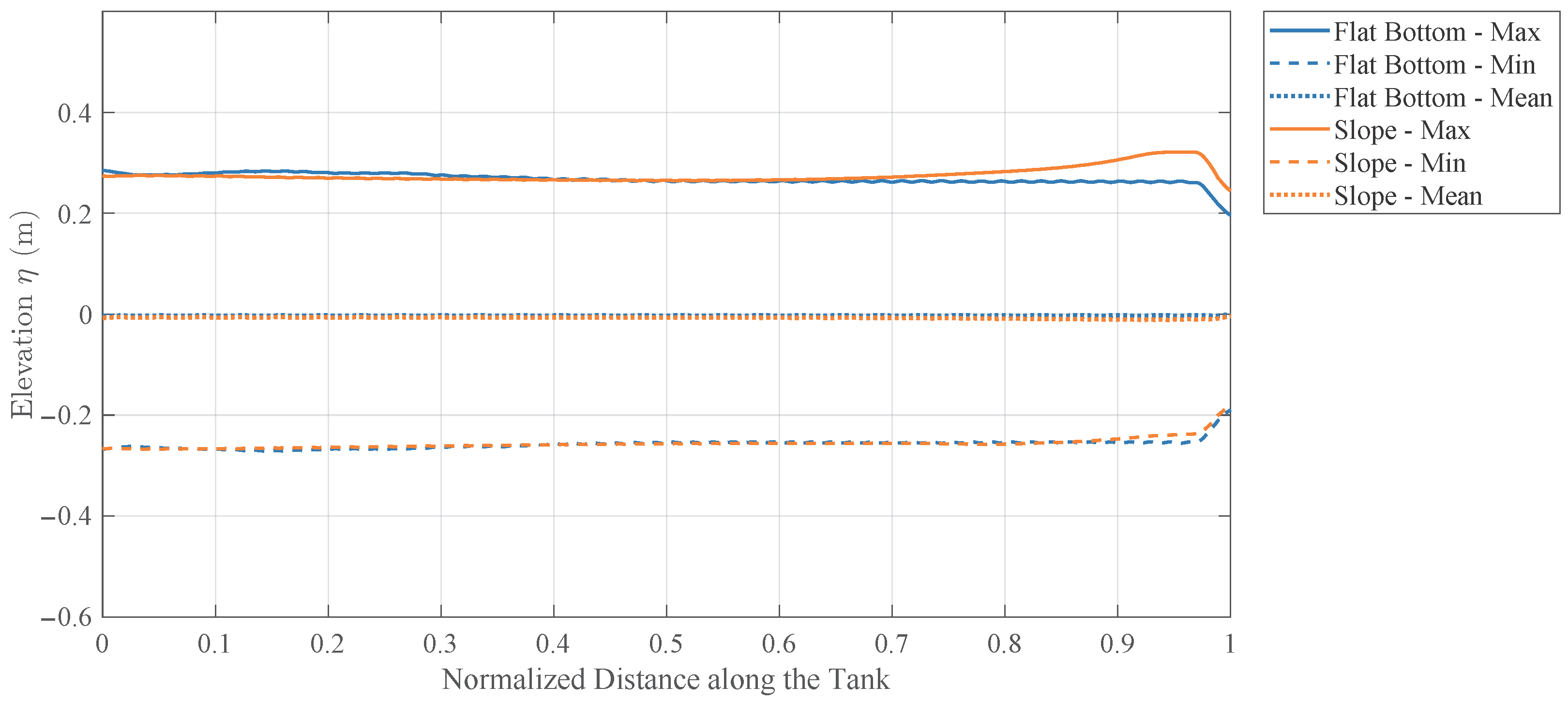
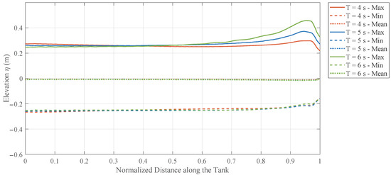
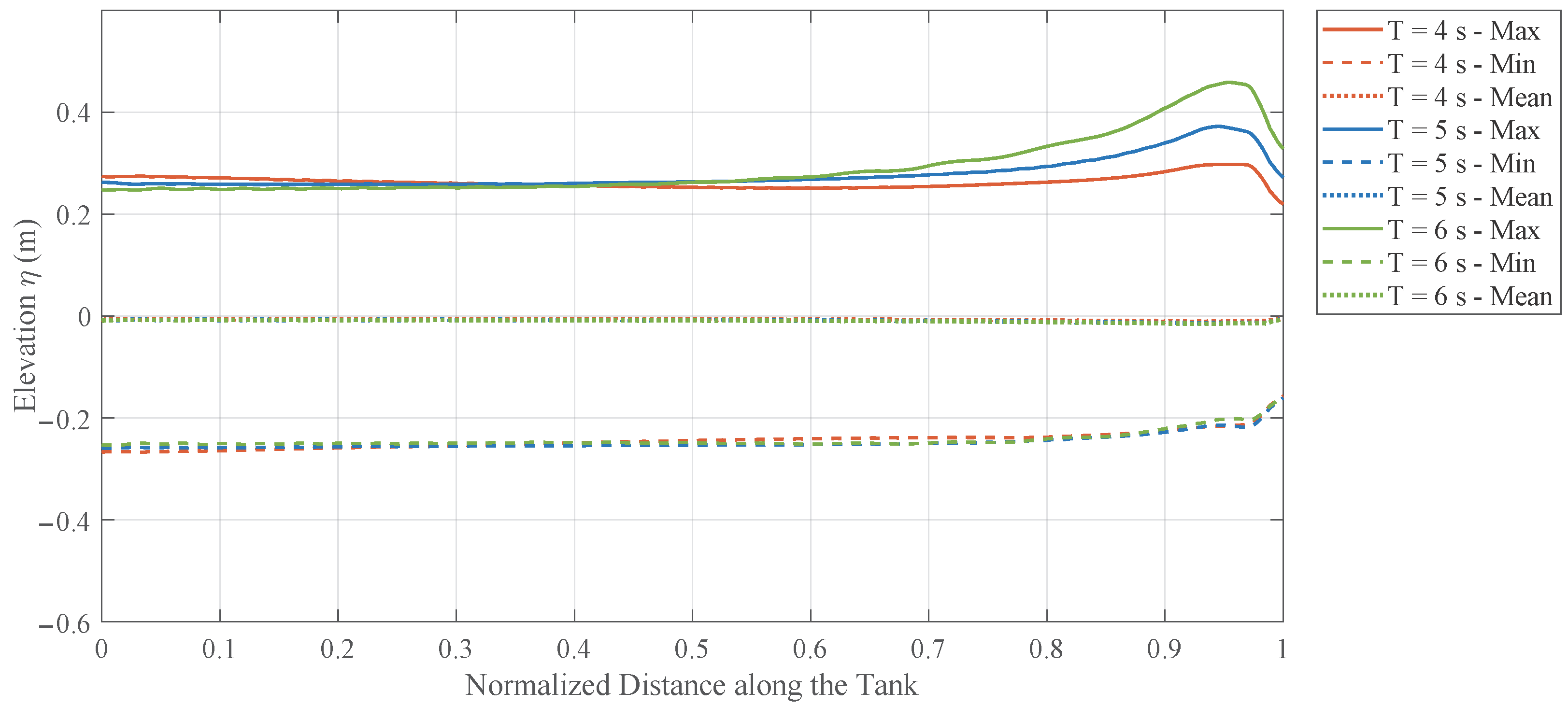
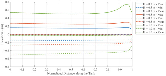
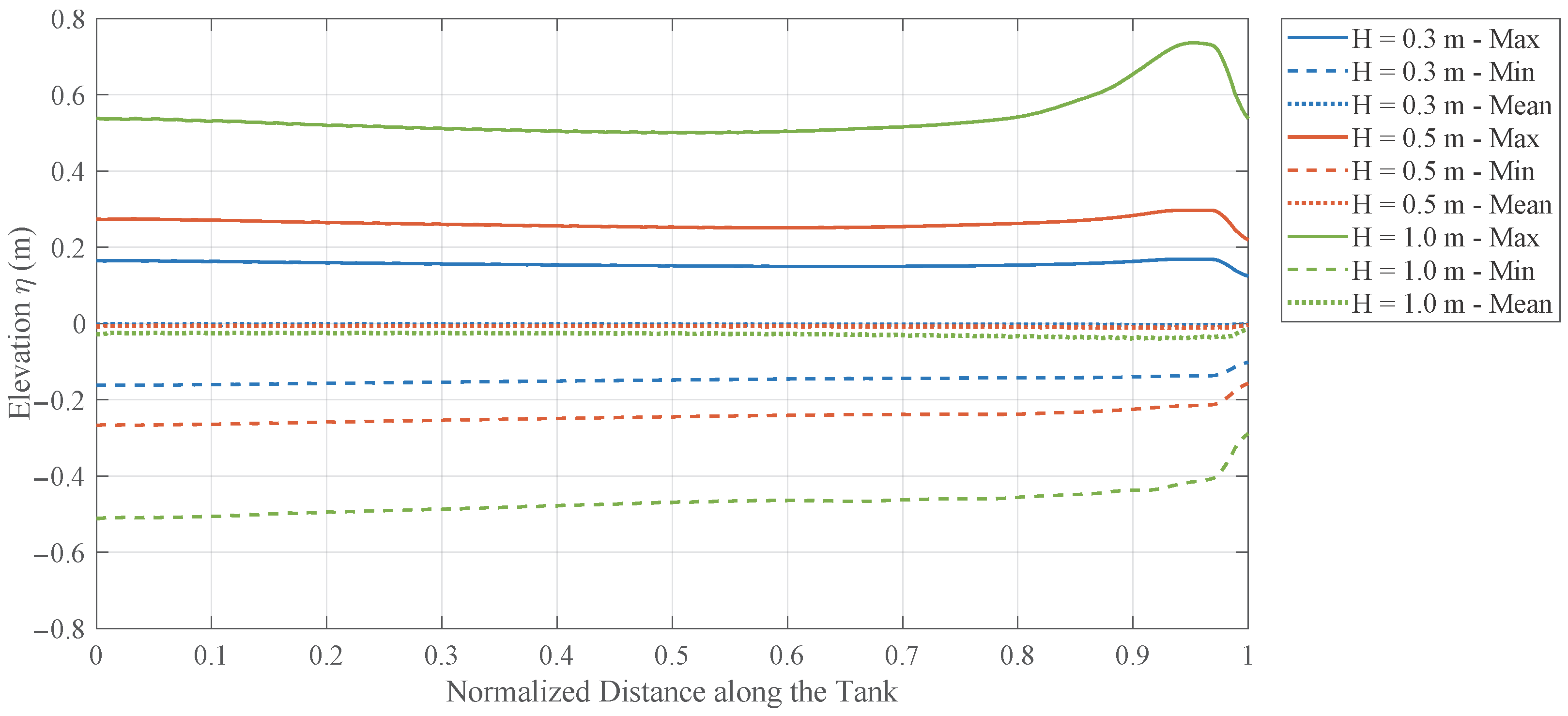
Figure 7, Figure 8 and Figure 9 provide parametric comparisons of the maximum, minimum, and mean free-surface elevations along the tank, showing how bathymetry, wave period, and incident wave height modify the shoaling process.

Figure 7. Comparison of along-tank wave-elevation envelopes (maximum, minimum, and mean values) for flat-bottom and sloping-bottom seabeds.

Figure 8. Comparison of along-tank wave-elevation envelopes (maximum, minimum, and mean values) for different wave periods ($T=4,5,6\mathrm{s}$) over the sloping-bottom seabed.

Figure 9. Comparison of along-tank wave-elevation envelopes (maximum, minimum, and mean values) for different incident wave heights at a fixed period ($T=4\mathrm{s}$) over the sloping-bottom seabed.

Figure 7 compares the wave envelopes over the flat-bottom and sloping-bottom bathymetries. Over most of the upstream region, the two cases almost coincide, indicating that the incoming wave train changes only weakly before reaching the shallower part of the domain. The difference becomes clear in the downstream section: the flat-bottom case remains nearly uniform, whereas the sloping-bottom case develops a noticeable rise in the upper envelope and a milder change in the lower envelope, with the strongest divergence appearing close to the shallow end. The mean water level stays close to zero in both cases, so the dominant bathymetric effect is not a large setup shift but a progressive crest amplification caused by shoaling over decreasing depth.

Figure 8 shows the effect of wave period for the sloping-bottom case. All three periods show limited variation over the deeper upstream part of the tank, followed by clear amplification after the waves enter the shallower region. The period dependence is systematic: $T=6\mathrm{s}$ produces the largest crest growth, $T=5\mathrm{s}$ is intermediate, and $T=4\mathrm{s}$ remains the weakest throughout the downstream reach. This ordering indicates that longer waves are more sensitive to the same depth transition and therefore undergo stronger shoaling, which leads to larger free-surface envelopes near the shoreward end.

Figure 9 shows that increasing the incident wave height primarily raises the envelope level over the entire domain, but the effect becomes much stronger in shallow water. The $H=1.0\mathrm{m}$ case exhibits a pronounced downstream crest increase that is much larger than the corresponding change in the trough envelope, while the $H=0.3\mathrm{m}$ and $H=0.5\mathrm{m}$ cases remain comparatively moderate. The mean water level shifts only slightly, so the main change is the increasing crest–trough asymmetry. This behavior indicates that larger incident waves experience stronger nonlinear deformation during shoaling, with crest amplification becoming increasingly dominant as the relative depth decreases.

These wave-evolution characteristics provide the spatially varying incident pressure field required for subsequent hydrodynamic analyses. In particular, the computed incident wave pressure is used to evaluate the excitation force $F_I$, while the corresponding normal velocities along the body surface serve as boundary conditions for the diffraction problem of each local module.

4.3. Hydrodynamic Coefficients over Variable Bathymetry

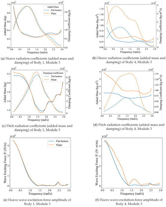
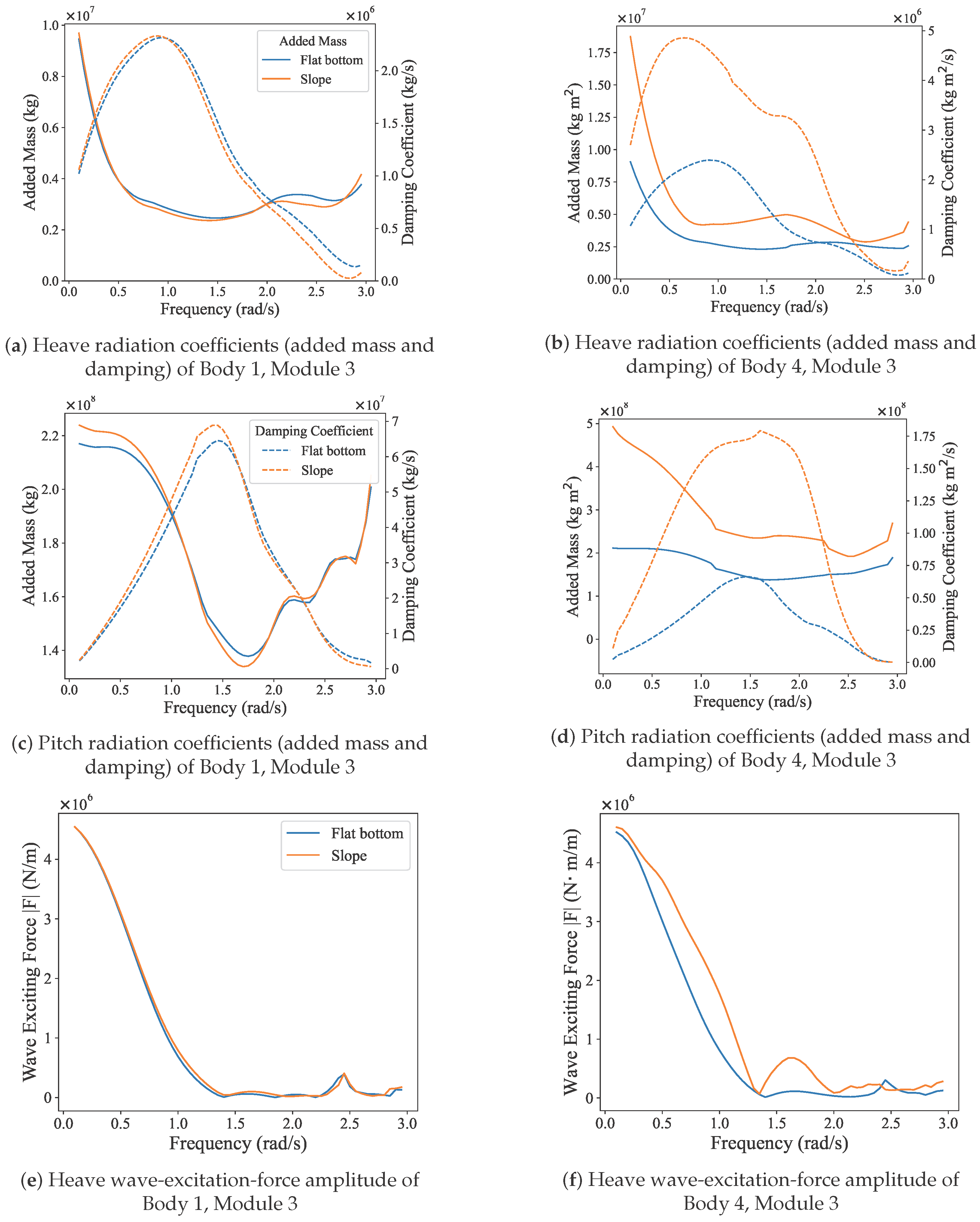
Frequency-domain hydrodynamic coefficients were computed for the flat-bottom and sloping-bottom seabed configurations defined in Table 2. Representative comparisons of radiation coefficients and wave-excitation amplitudes are presented in Figure 10 for an upstream location (Body 1, Module 3) and a downstream location (Body 4, Module 3). The comparisons include heave and pitch radiation coefficients (added mass and radiation damping) as well as the heave excitation-force amplitude. The plotted quantities are reported for the same module location in the two bathymetric configurations.

Figure 10. Comparison of frequency-domain hydrodynamic characteristics for Body 1 and Body 4 at Module 3 under different seabed profiles (flat bottom and slope): (a,b) heave radiation coefficients (added mass and damping), (c,d) pitch radiation coefficients (added mass and damping), and (e,f) heave wave-excitation-force amplitudes.

The results indicate a pronounced sensitivity to local water depth. At the upstream position (Body 1, Module 3), which remains in relatively deep water, the added mass, radiation damping, and excitation-force amplitudes obtained for the flat-bottom and sloping-bottom cases are generally very close over the investigated frequency range. In contrast, at the downstream position (Body 4, Module 3), located in shallower water, clear deviations from the flat-bottom reference are observed, including changes in the magnitude of added mass and shifts in the damping characteristics at several frequencies. These trends demonstrate that local depth conditions play a dominant role in shaping the frequency-dependent hydrodynamic behavior of the modular floating structure.

Another important feature is the smooth frequency variation of the computed coefficients across the full frequency band considered ($0.1$–$3.0\mathrm{rad}/\mathrm{s}$). The Rankine-source boundary element formulation yields continuous added-mass, damping, and excitation-force curves without spurious oscillations, which is particularly advantageous for subsequent transformation into time-domain retardation functions within the Cummins framework. The numerical smoothness of these frequency-domain coefficients improves the robustness of the hydroelastic time-domain simulations and reduces the risk of artificial contamination in the convolution-based radiation-force evaluation.

In addition, the comparisons between the upstream and downstream modules highlight the spatial variability of the hydrodynamic response within the multi-module system. The observed differences in local radiation and excitation characteristics imply that hydrodynamic coupling effects are not uniform along the structure, but instead depend on module position and surrounding depth conditions. This spatially varying behavior provides further justification for the discrete-module assembly adopted in the present hydroelastic model, in which module-level hydrodynamic properties are retained in the time-domain calculation.

4.4. Hydroelastic Response

To provide a unified interpretation of structural behavior, hydroelastic motions and bending moments are discussed through three sets of comparisons: flat-bottom versus sloped-bottom bathymetry under different wave periods, flat-bottom versus sloped-bottom bathymetry under different wave heights, and rigid-body versus hydroelastic modelling to assess structural elasticity. In the period and wave-height comparisons, flat-bottom and sloped-bottom results are plotted together, with flat-bottom cases shown by dashed lines. Heave and bending-moment RMS distributions are analyzed consistently to identify coupled response trends.

4.4.1. Effects of Wave Period

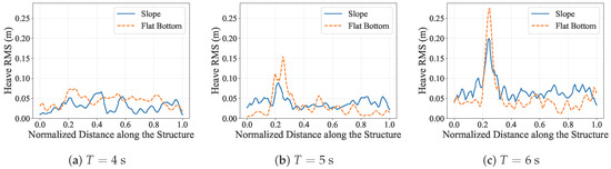
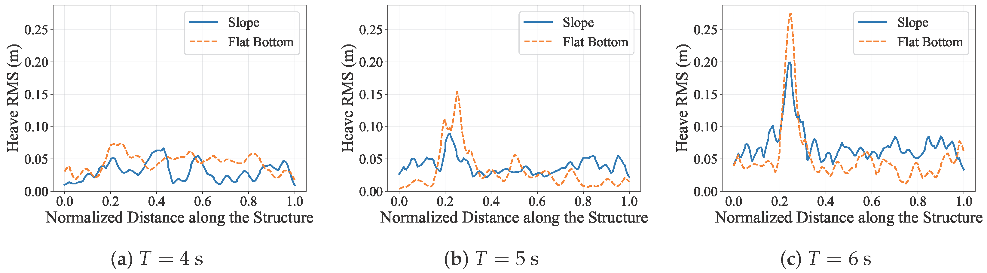
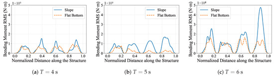
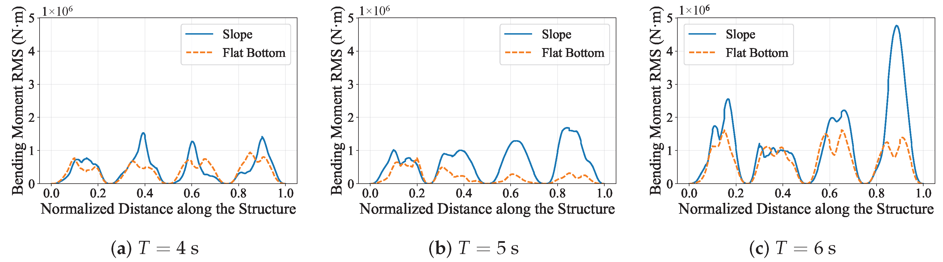
Figure 11 and Figure 12 present hydroelastic heave and bending-moment RMS responses for $T=4$, 5, and $6\mathrm{s}$ at a fixed incident wave height of $H=0.5\mathrm{m}$, with flat-bottom and sloped-bottom results shown separately in each period panel. The heave response again shows stronger spatial non-uniformity under sloped bathymetry, while the bending-moment response reveals a clearer load amplification effect associated with terrain-induced shoaling.

Figure 11. Comparison of hydroelastic heave RMS distributions under flat-bottom and sloped-bottom bathymetries for different wave periods at $H=0.5\mathrm{m}$.

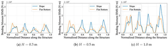
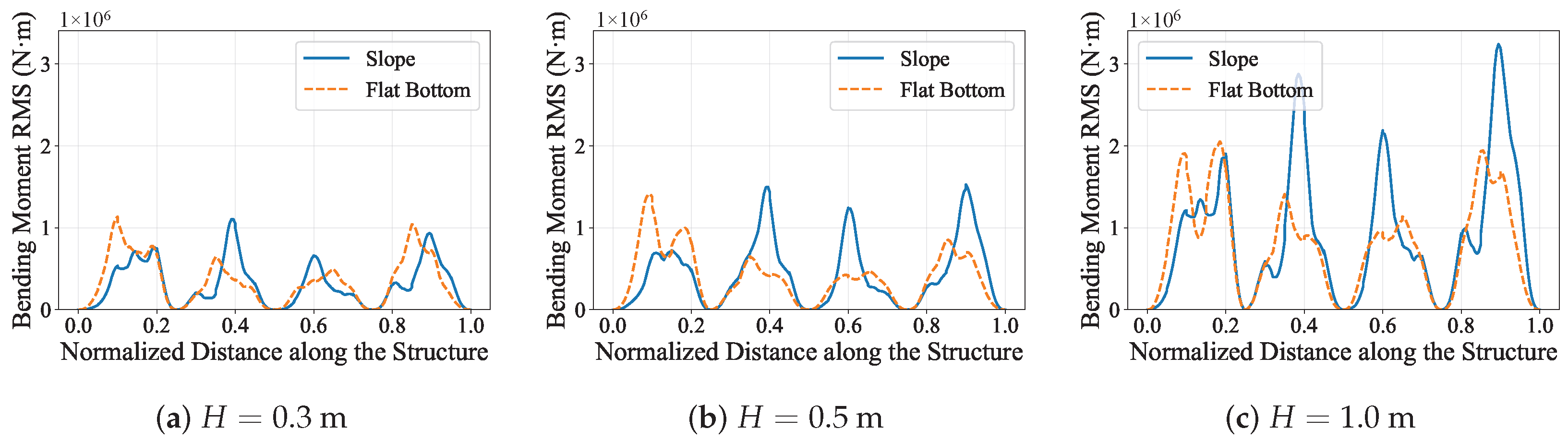
Figure 12. Comparison of bending-moment RMS distributions under flat-bottom and sloped-bottom bathymetries for different wave periods at $H=0.5\mathrm{m}$.

A clear period ranking is observed in the bending moments. At $T=4\mathrm{s}$, the two bathymetries remain mixed, but the sloped-bottom case already produces sharper peaks near the middle and downstream parts of the structure. At $T=5\mathrm{s}$, the sloped-bottom curve exceeds the flat-bottom curve over most of the structure, and the downstream amplification becomes more pronounced. At $T=6\mathrm{s}$, the response strengthens further, with the largest bending-moment peak developing near the downstream end under sloped bathymetry. This progressive increase in RMS level and spatial concentration is consistent with the stronger shoaling trends shown in Figure 8.

The strongest response in the long-period case is physically consistent with the identified two-node bending natural period of the structure (approximately $6.17\mathrm{s}$), suggesting that period-dependent shoaling and structural dynamic sensitivity act jointly to elevate hydroelastic demand. Overall, the results indicate that wave period governs not only the absolute heave level but also the magnitude and localization of the bending moment, while terrain effects further magnify this period sensitivity.

4.4.2. Effects of Wave Height

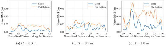
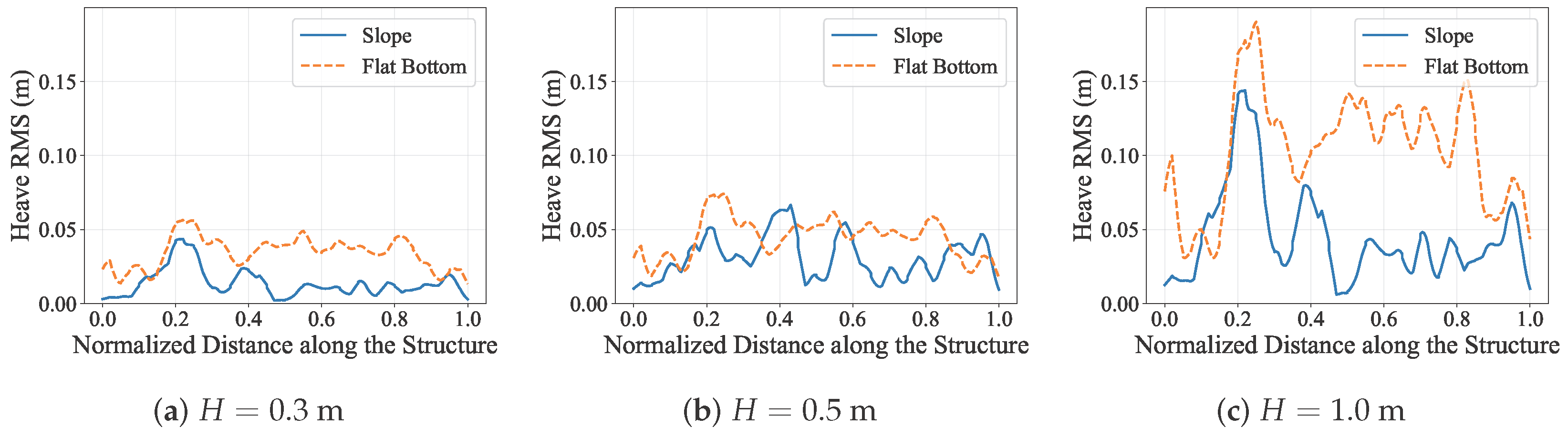
At a fixed period ($T=4\mathrm{s}$), Figure 13 and Figure 14 compare hydroelastic heave and bending-moment RMS responses for incident wave heights of $H=0.3$, $0.5$, and $1.0\mathrm{m}$ under the two bathymetric conditions. Both responses increase with incident wave height, but the amplification is clearly nonlinear, especially in the larger-H cases where the response growth is accompanied by stronger spatial redistribution along the structure.

Figure 13. Comparison of hydroelastic heave RMS distributions under flat-bottom and sloped-bottom bathymetries for different incident wave heights at $T=4\mathrm{s}$.

Figure 14. Comparison of bending-moment RMS distributions under flat-bottom and sloped-bottom bathymetries for different incident wave heights at $T=4\mathrm{s}$.

The heave response increases nonlinearly with incident wave height under both bathymetries. Physically, this behavior reflects the fact that increasing H strengthens finite-amplitude wave effects, so the hydrodynamic loading no longer scales linearly with the incident surface elevation. As wave height grows, the pressure field acting on the underside of the structure becomes more asymmetric over a wave cycle, while wave transformation over the slope modifies the local phase and amplitude of the excitation along the body. The $H=1.0\mathrm{m}$ case is therefore not simply a scaled-up version of the lower-height cases; instead, it shows much stronger amplification in the upstream part of the structure and a more uneven response distribution overall. In terms of terrain dependence, the flat-bottom case remains larger over much of the structure for $H=0.3\mathrm{m}$ and becomes clearly dominant again over most of the span at $H=1.0\mathrm{m}$, whereas the $H=0.5\mathrm{m}$ case exhibits a mixed pattern with localized sloped-bottom amplification in the middle and near the downstream end. This mixed behavior suggests that bathymetry influences heave through two competing mechanisms: shoaling over the slope tends to increase local excitation in shallower regions, whereas the accompanying change in wavelength and phase can also reduce coherence of the vertical forcing over the full structure. As a result, the net heave response is governed not only by local wave amplification, but also by how efficiently the distributed wave loading projects onto the dominant global deformation pattern.

The bending-moment response also grows nonlinearly with wave height, but the bathymetric effect is stronger and more localized than in the heave response. This is physically expected because bending moment depends on spatial gradients of displacement and load, not only on the absolute motion amplitude. Once wave shoaling over the slope increases the local wave steepness, the excitation becomes more uneven along the structure, and the resulting differential support from the surrounding water enhances curvature demand between adjacent modules. The sloped-bottom case therefore produces a more non-uniform bending-moment distribution, with clearly larger peaks near the middle and downstream regions, whereas the flat-bottom case is generally larger in the upstream region. At $H=0.3\mathrm{m}$, the two bathymetries are still relatively mixed, although the slope case already develops a distinct mid-structure peak. At $H=0.5\mathrm{m}$, the slope case clearly exceeds the flat-bottom case in the middle and downstream parts of the structure while the flat-bottom case retains larger upstream peaks. At $H=1.0\mathrm{m}$, this contrast becomes strongest, with pronounced sloped-bottom maxima in the middle region and especially near the downstream end. These results indicate that larger incident waves intensify bending demand much more strongly than they increase the overall heave level, because terrain-induced wave amplification is converted primarily into internal load concentration rather than into a uniform rigid-body-type response.

4.4.3. Comparison Between Hydroelastic and Rigid-Body Responses

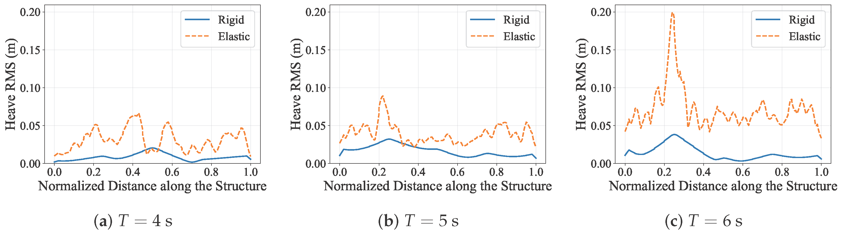
To assess the role of structural elasticity in the coupled response, RMS distributions are compared between rigid-body and hydroelastic configurations for sloped-bathymetry cases with a fixed incident wave height of $H=0.5\mathrm{m}$ and wave periods $T=4$, 5, and $6\mathrm{s}$. Figure 15 and Figure 16 present the corresponding heave and bending-moment RMS distributions.

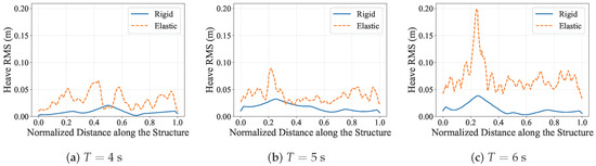
Figure 15. Comparison of heave RMS distributions between rigid-body and hydroelastic configurations for sloped-bathymetry cases with $H=0.5\mathrm{m}$ and $T=4$, 5, and $6\mathrm{s}$.

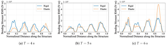
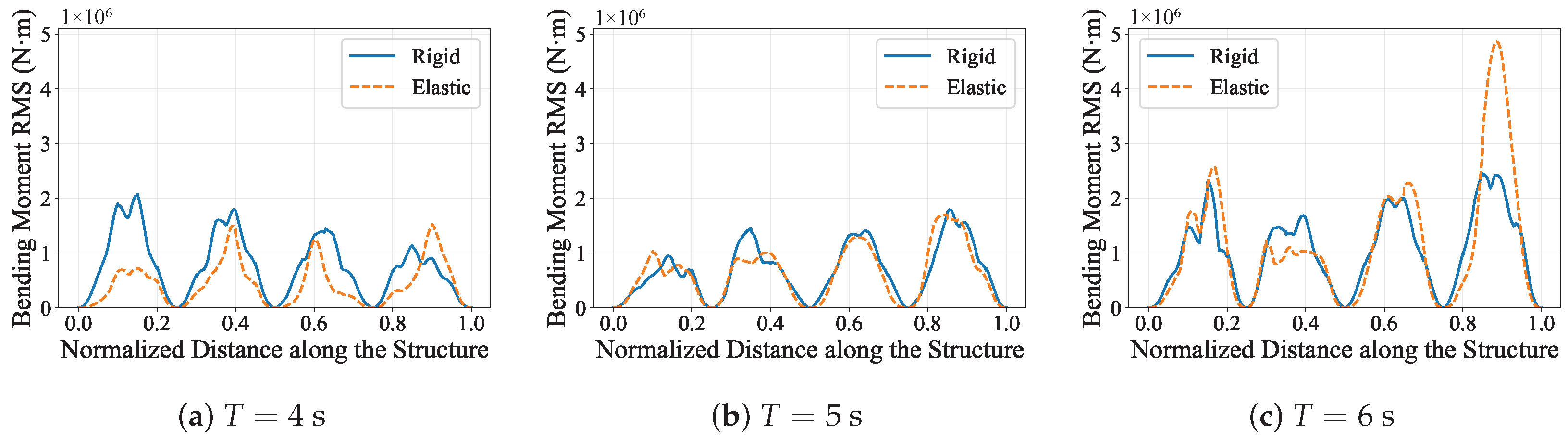
Figure 16. Comparison of bending-moment RMS distributions between rigid-body and hydroelastic configurations for sloped-bathymetry cases with $H=0.5\mathrm{m}$ and $T=4$, 5, and $6\mathrm{s}$.

Across all three periods, introducing hydroelastic effects strongly increases the heave response relative to the rigid-body reference. The elastic curves remain above the rigid-body curves over nearly the entire structure for $T=4$, 5, and $6\mathrm{s}$, and the separation becomes particularly pronounced in the long-period case, where the elastic model produces much larger upstream and distributed response levels.

The bending-moment response exhibits a different pattern from the heave response. At $T=4\mathrm{s}$, the rigid-body model produces larger RMS levels over most of the structure, although the hydroelastic case becomes larger near the downstream peak. At $T=5\mathrm{s}$, the rigid and hydroelastic bending-moment distributions remain close over most of the span, indicating only limited elastic redistribution. At $T=6\mathrm{s}$, however, the comparison becomes strongly mixed and the hydroelastic model develops a much larger downstream peak than the rigid-body result. These results show that elasticity does not simply increase every response component; rather, it redistributes wave-induced demand between global motion and structural bending.

The stronger rigid-versus-hydroelastic differences in the longer-period case are physically consistent with the previously identified structural dynamic sensitivity near the two-node bending natural period. Overall, these comparisons confirm that modelling structural elasticity has a first-order influence on both global motions and bending-moment transfer and should therefore be retained explicitly in time-domain hydroelastic assessment.

4.5. Design Implications

The numerical results suggest several design implications for nearshore large floating structures deployed over variable bathymetry. First, the governing design condition should not be identified only from the largest global motion response. In the present results, the bathymetric slope often increases bending-moment concentration more clearly than it increases overall heave, meaning that a configuration appearing acceptable in terms of motion comfort or operability may still experience critical structural demand in modules located above transitional or shallow regions.

Second, local seabed variation should be treated as a primary design parameter rather than a secondary site descriptor. The response patterns show that the slope changes not only the response magnitude but also the position of the dominant load peaks. For engineering practice, this means that connector details, module interfaces, and other structurally sensitive regions should be checked against location-specific load redistribution associated with shoaling, especially near the middle and downstream portions of the structure where amplified bending peaks repeatedly emerge.

Third, period-dependent structural sensitivity must be considered together with bathymetric wave transformation. The strongest load amplification occurs when long-wave excitation over the slope acts in combination with the structural natural period, so screening based on wave height alone is insufficient. From a design standpoint, this supports using hydroelastic analyses that preserve both spatially varying hydrodynamic coefficients and elastic deformation, particularly for shallow-water sites where depth-induced wave transformation is pronounced. More broadly, the results indicate that practical mitigation may require coordinated adjustment of structural stiffness, module layout, and site selection to reduce the coincidence between shoaling-enhanced excitation zones and dynamically sensitive portions of the floating system.

5. Conclusions

This study presented a time-domain hydroelastic framework that combines the fully nonlinear non-hydrostatic wave solver NHWAVE with a variable-depth Rankine-source radiation–diffraction model and a discrete-module Cummins formulation. The approach enables consistent simulation of nonlinear wave evolution, spatially varying hydrodynamic coefficients, and elastic-body dynamics for large floating infrastructures in shallow water.

The computed hydrodynamic coefficients and time-domain responses show strong depth dependence, with clear module-to-module variability under sloped bathymetry and smooth frequency-domain behavior suitable for robust convolution-based radiation-force evaluation.

Parametric simulations of a $600\mathrm{m}$ modular floating structure were used primarily to examine how varying bathymetry modifies the hydroelastic response under representative regular-wave conditions. Transitioning from a flat seabed to a slope with $tan\alpha =0.0133$ amplified shoaling, increased bending-moment RMS responses, and introduced strong spatial non-uniformity in the hydroelastic motions and bending-demand distribution along the structure. The additional wave-period and wave-height cases show that this bathymetry-induced amplification persists across the tested wave conditions, with longer-period waves producing the largest bending demand and larger incident heights intensifying the nonlinear growth of motions and bending moments, particularly in modules situated over shallower sections. Additional rigid-body versus hydroelastic comparisons at fixed $H=0.5\mathrm{m}$ and $T=4$–$6\mathrm{s}$ showed clear period-dependent redistribution of motion and bending-moment RMS responses, with the largest rigid-versus-hydroelastic differences in the longer-period cases near structural dynamic sensitivity. These results underscore the need for explicit hydroelastic modeling rather than a rigid-body idealization.

Overall, the findings demonstrate that accurate design assessments for nearshore large floating structures must resolve local bathymetry under the expected wave conditions while explicitly accounting for structural elasticity effects. Future work will extend the framework to multi-directional irregular seas and more complex structural layouts, providing broader guidance for large floating structures subjected to nonlinear shallow-water waves.

Appendix A.1. Mesh Convergence Test

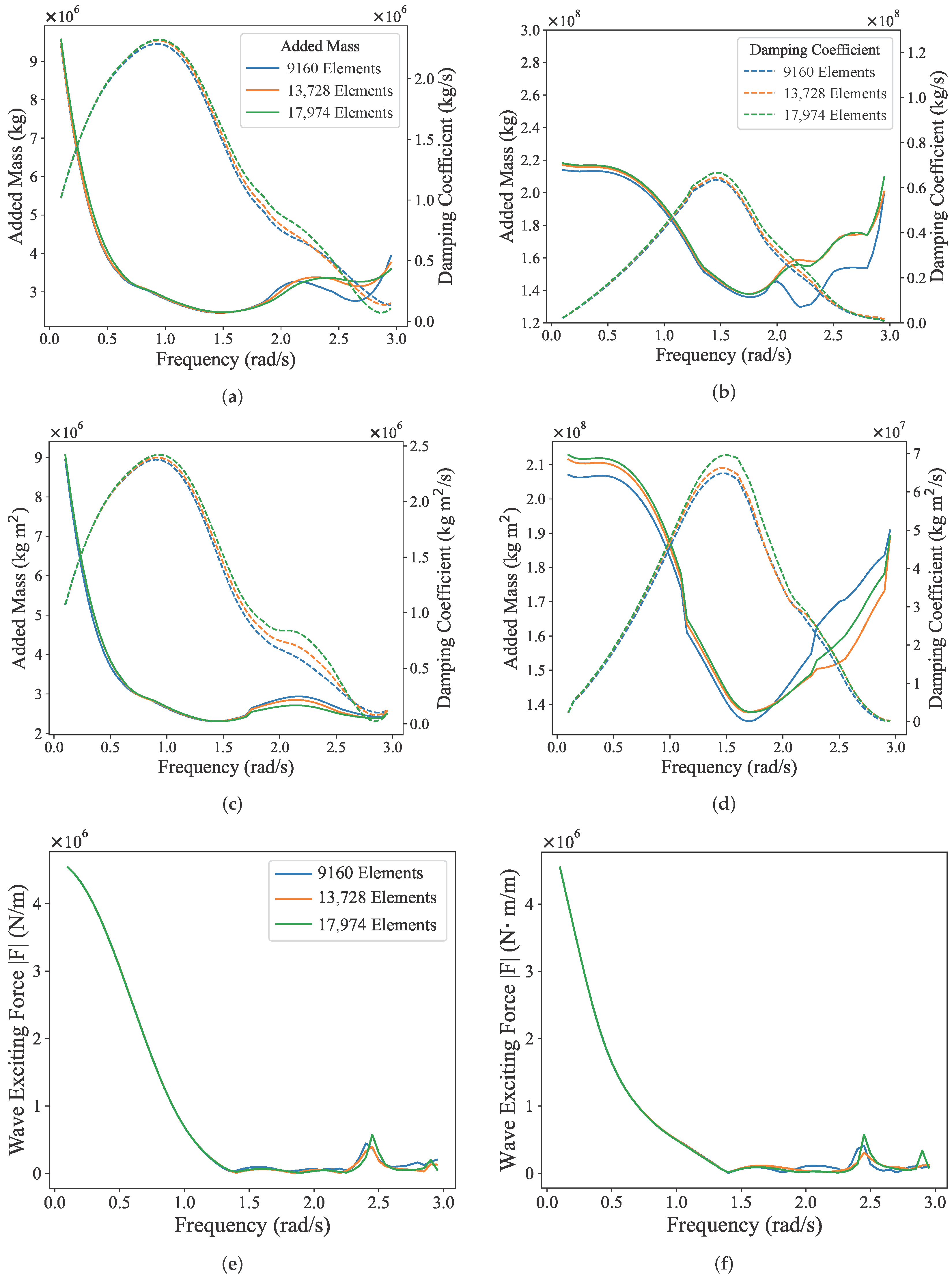
For the multi-body case, three boundary-element discretizations with 9160, 13,728, and 17,974 panels are compared under the same flat-bottom condition used for the WAMIT comparison. Figure A1 presents representative results for Body 1, Module 3 and Body 4, Module 3, including heave and pitch radiation coefficients as well as the heave wave-excitation force.

The results show that once the panel number reaches 13,728, the computed curves are already very close to those obtained with 17,974 panels, indicating satisfactory convergence of the hydrodynamic solution for the multi-body configuration. To retain sufficient accuracy in the subsequent response analysis, the calculations reported in the main text are based on the 17,974-panel discretization.

Figure A1. Mesh convergence test for the multi-body case. (a) Heave radiation coefficients (added mass and damping) of Body 1, Module 3. (b) Pitch radiation coefficients (added mass and damping) of Body 1, Module 3. (c) Heave radiation coefficients (added mass and damping) of Body 4, Module 3. (d) Pitch radiation coefficients (added mass and damping) of Body 4, Module 3. (e) Heave wave-excitation force of Body 1, Module 3. (f) Heave wave-excitation force of Body 4, Module 3.

Figure A1. Mesh convergence test for the multi-body case. (a) Heave radiation coefficients (added mass and damping) of Body 1, Module 3. (b) Pitch radiation coefficients (added mass and damping) of Body 1, Module 3. (c) Heave radiation coefficients (added mass and damping) of Body 4, Module 3. (d) Pitch radiation coefficients (added mass and damping) of Body 4, Module 3. (e) Heave wave-excitation force of Body 1, Module 3. (f) Heave wave-excitation force of Body 4, Module 3.

Appendix A.2. Validation of Hydrodynamic Coefficients

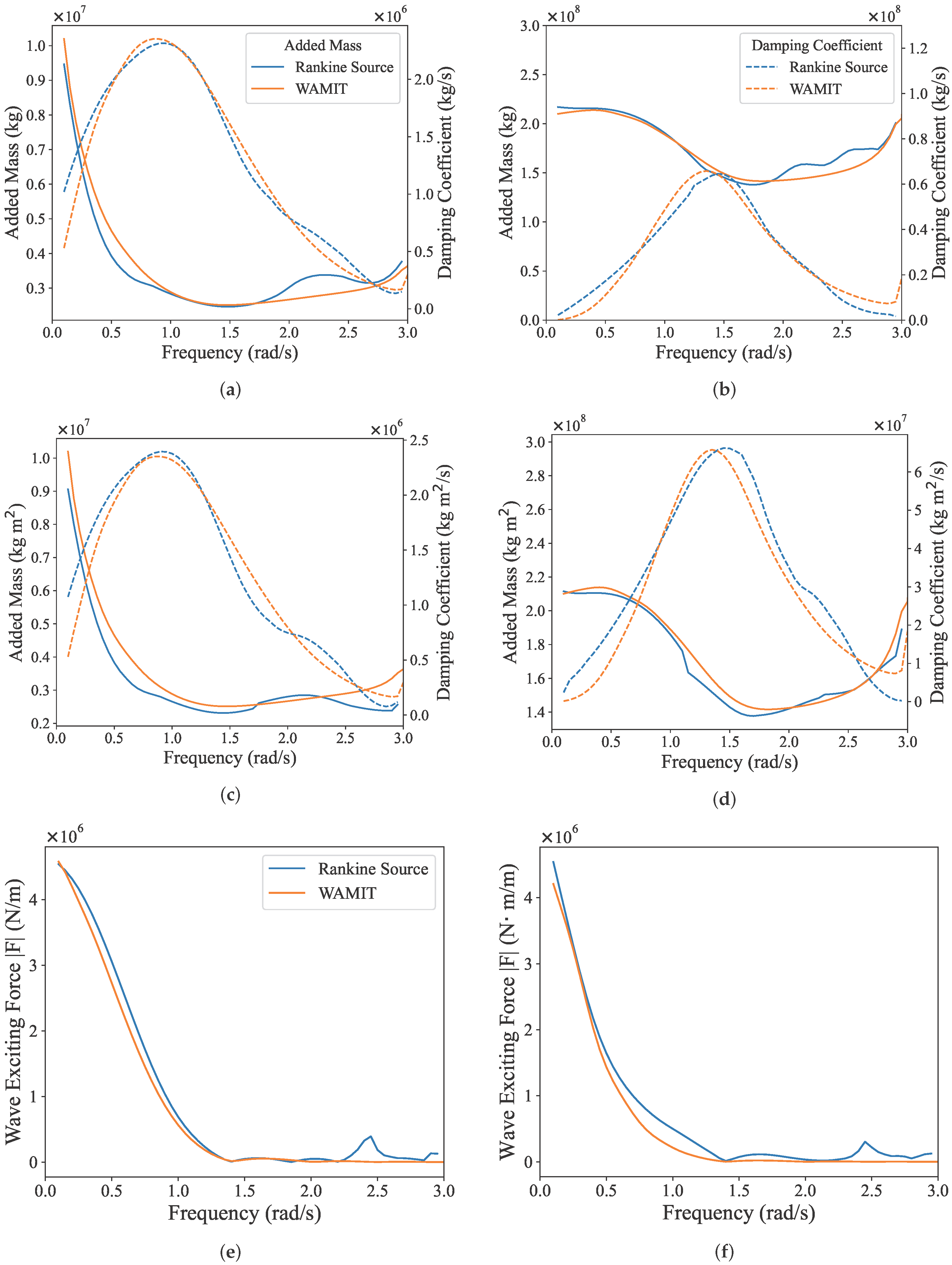
Based on the converged mesh, Figure A2 compares the present multi-body results with those obtained from WAMIT for the flat-bottom case. Overall, good agreement is observed over the main frequency range for both radiation coefficients and excitation-force amplitudes, indicating that the present method captures the essential radiation and diffraction coupling effects within the multi-body system.

Figure A2. Validation of the multi-body hydrodynamic results against WAMIT. (a) Heave radiation coefficients (added mass and damping) of Body 1, Module 3. (b) Pitch radiation coefficients (added mass and damping) of Body 1, Module 3. (c) Heave radiation coefficients (added mass and damping) of Body 4, Module 3. (d) Pitch radiation coefficients (added mass and damping) of Body 4, Module 3. (e) Heave wave-excitation force of Body 1, Module 3. (f) Heave wave-excitation force of Body 4, Module 3.

Figure A2. Validation of the multi-body hydrodynamic results against WAMIT. (a) Heave radiation coefficients (added mass and damping) of Body 1, Module 3. (b) Pitch radiation coefficients (added mass and damping) of Body 1, Module 3. (c) Heave radiation coefficients (added mass and damping) of Body 4, Module 3. (d) Pitch radiation coefficients (added mass and damping) of Body 4, Module 3. (e) Heave wave-excitation force of Body 1, Module 3. (f) Heave wave-excitation force of Body 4, Module 3.

References

- Liu, G.; Guo, J.; Peng, H.; Ping, H.; Ma, Q. Review of Recent Offshore Floating Photovoltaic Systems. J. Mar. Sci. Eng. 2024, 12, 1942. [Google Scholar] [CrossRef] [Scilit]
- Chen, Y.; Zhang, Y.; Tian, X.; Guo, X.; Li, X.; Zhang, X. A Numerical Framework for Hydroelastic Analysis of a Flexible Floating Structure under Unsteady External Excitations: Motion and Internal Force/Moment. Ocean Eng. 2022, 253, 111288. [Google Scholar] [CrossRef] [Scilit]
- Shi, Y.; Wei, Y.; Tay, Z.Y.; Chen, Z. Hydroelastic Analysis of Offshore Floating Photovoltaic Based on Frequency-Domain Model. Ocean Eng. 2023, 289, 116213. [Google Scholar] [CrossRef] [Scilit]
- Li, S.; Moan, T.; Fu, S.; Zhang, S.; Xu, Y. Hydroelastic Analysis of a Floating Bridge under Spatially Inhomogeneous Waves, with Emphasis on the Effect of Drift Force Modeling. Appl. Ocean Res. 2023, 139, 103666. [Google Scholar] [CrossRef] [Scilit]
- Zhang, Y.; Zhang, X.; Chen, Y.; Tian, X.; Li, X. A Frequency-Domain Hydroelastic Analysis of a Membrane-Based Offshore Floating Photovoltaic Platform in Regular Waves. J. Fluids Struct. 2024, 127, 104125. [Google Scholar] [CrossRef] [Scilit]
- Shi, Y.; Wei, Y.; Chen, K.; Xin, C.; Tay, Z.Y.; Chen, Z. Frequency-Domain Approach of Hydroelastic Response for Flexible Offshore Floating Photovoltaic under Combined Wind and Wave Loads. Ocean Eng. 2025, 323, 120565. [Google Scholar] [CrossRef] [Scilit]
- Chen, Y.; Zhang, X.; Shen, K.; Ren, X. Extension of the Discrete-Module-Finite-Element Method into the Interconnected Large Floating Flexible Structures. Ocean Eng. 2023, 269, 113549. [Google Scholar] [CrossRef] [Scilit]
- Wang, C.; Cui, M.; Cheng, Z.; Moan, T. A Review on Design and Analysis of Floating Bridges: Numerical Simulations, Model Tests and Field Measurements. Ocean Eng. 2024, 306, 118065. [Google Scholar] [CrossRef] [Scilit]
- Hwang, J.H.; Van, S.P.; Choi, B.J.; Chang, Y.S.; Kim, Y.H. The Physical Processes in the Yellow Sea. Ocean Coast. Manag. 2014, 102, 449–457. [Google Scholar] [CrossRef] [Scilit]
- Murray, N.J.; Ma, Z.; Fuller, R.A. Tidal Flats of the Yellow Sea: A Review of Ecosystem Status and Anthropogenic Threats. Austral Ecol. 2015, 40, 472–481. [Google Scholar] [CrossRef] [Scilit]
- Chang, M.; Li, P.; Li, Z.; Wang, H. Mapping Tidal Flats of the Bohai and Yellow Seas Using Time Series Sentinel-2 Images and Google Earth Engine. Remote Sens. 2022, 14, 1789. [Google Scholar] [CrossRef] [Scilit]
- Ding, J.; Tian, C.; Wu, Y.s.; Li, Z.w.; Ling, H.j.; Ma, X.z. Hydroelastic Analysis and Model Tests of a Single Module VLFS Deployed near Islands and Reefs. Ocean Eng. 2017, 144, 224–234. [Google Scholar] [CrossRef] [Scilit]
- Newman, J.N.; Lee, C.H. Boundary-Element Methods in Offshore Structure Analysis. J. Offshore Mech. Arct. Eng. 2002, 124, 81–89. [Google Scholar] [CrossRef] [Scilit]
- Athanassoulis, G.A.; Belibassakis, K.A. A Consistent Coupled-Mode Theory for the Propagation of Small-Amplitude Water Waves over Variable Bathymetry Regions. J. Fluid Mech. 1999, 389, 275–301. [Google Scholar] [CrossRef] [Scilit]
- Newman, J. The Theory of Ship Motions; Elsevier: Amsterdam, The Netherlands, 1979; pp. 221–283. [Google Scholar] [CrossRef] [Scilit]
- Madsen, P.A.; Banijamali, B.; Schäffer, H.A.; Sørensen, O.R. Boussinesq Type Equations with High Accuracy in Dispersion and Nonlinearity. In Coastal Engineering 1996; American Society of Civil Engineers (ASCE): Reston, VA, USA, 2015; pp. 95–108. [Google Scholar] [CrossRef] [Scilit]
- Madsen, P.A.; Murray, R.; Sørensen, O.R. A New Form of the Boussinesq Equations with Improved Linear Dispersion Characteristics. Coast. Eng. 1991, 15, 371–388. [Google Scholar] [CrossRef] [Scilit]
- Madsen, P.A.; Sørensen, O.R. A New Form of the Boussinesq Equations with Improved Linear Dispersion Characteristics. Part 2. A Slowly-Varying Bathymetry. Coast. Eng. 1992, 18, 183–204. [Google Scholar] [CrossRef] [Scilit]
- Ding, J.; Tian, C.; Wu, Y.s.; Wang, X.f.; Liu, X.l.; Zhang, K. A Simplified Method to Estimate the Hydroelastic Responses of VLFS in the Inhomogeneous Waves. Ocean Eng. 2019, 172, 434–445. [Google Scholar] [CrossRef] [Scilit]
- Yang, P.; Li, Z.; Wu, Y.; Wen, W.; Ding, J.; Zhang, Z. Boussinesq-Hydroelasticity Coupled Model to Investigate Hydroelastic Responses and Connector Loads of an Eight-Module VLFS near Islands in Time Domain. Ocean Eng. 2019, 190, 106418. [Google Scholar] [CrossRef] [Scilit]
- Jiang, C.; El Moctar, O.; Zhang, G. Nonlinear Modeling of Wave–Structure Interaction for a Flexible Floating Structure. Ocean Eng. 2024, 300, 117489. [Google Scholar] [CrossRef] [Scilit]
- Ma, G.; Shi, F.; Kirby, J.T. Shock-Capturing Non-Hydrostatic Model for Fully Dispersive Surface Wave Processes. Ocean Model. 2012, 43–44, 22–35. [Google Scholar] [CrossRef] [Scilit]
- Xiang, S.; Cheng, B.; Zhang, F.y.; Tang, M. An Improved Time Domain Approach for Analysis of Floating Bridges Based on Dynamic Finite Element Method and State-Space Model. China Ocean Eng. 2022, 36, 682–696. [Google Scholar] [CrossRef] [Scilit]
- Wei, W.; Fu, S.; Moan, T.; Lu, Z.; Deng, S. A Discrete-Modules-Based Frequency Domain Hydroelasticity Method for Floating Structures in Inhomogeneous Sea Conditions. J. Fluids Struct. 2017, 74, 321–339. [Google Scholar] [CrossRef] [Scilit]
- Wei, W.; Fu, S.; Moan, T.; Song, C.; Ren, T. A Time-Domain Method for Hydroelasticity of Very Large Floating Structures in Inhomogeneous Sea Conditions. Mar. Struct. 2018, 57, 180–192. [Google Scholar] [CrossRef] [Scilit]
- Cummins, W.E. The Impulse Response Function and Ship Motions. In Proceedings of the Symposium on Ship Theory at the Institut flir Schiffbau der Universitit Hamburg, Hamburg, Germany, 25–27 January 1962. [Google Scholar]
- Phillips, N.A. A Coordinate System Having Some Special Advantages for Numerical Forecasting. J. Meteorol. 1957, 14, 184–185. [Google Scholar] [CrossRef] [Scilit]
- Lin, P.; Li, C.W. A σ-coordinate Three-dimensional Numerical Model for Surface Wave Propagation. Int. J. Numer. Methods Fluids 2002, 38, 1045–1068. [Google Scholar] [CrossRef] [Scilit]
- Derakhti, M.; Kirby, J.T.; Shi, F.; Ma, G. NHWAVE: Consistent Boundary Conditions and Turbulence Modeling. Ocean Model. 2016, 106, 121–130. [Google Scholar] [CrossRef] [Scilit]
- Dean, R.G.; Dalrymple, R.A. Water Wave Mechanics for Engineers and Scientists; Advanced Series on Ocean Engineering; World Scientific: Singapore, 1991; Volme 2. [Google Scholar] [CrossRef]
- Holthuijsen, L.H. Waves in Oceanic and Coastal Waters, 1st ed.; Cambridge University Press: Cambridge, UK, 2007. [Google Scholar] [CrossRef] [Scilit]
- Hasselmann, K.F.; Barnett, T.P.; Bouws, E.; Carlson, H.C.; Cartwright, D.E.; Enke, K.; Ewing, J.A.; Gienapp, H.; Hasselmann, D.E.; Kruseman, P.; et al. Measurements of Wind-Wave Growth and Swell Decay During the Joint North Sea Wave Project (JONSWAP); Deutsches Hydrographisches Institut: Hamburg, Germany, 1973. [Google Scholar]
- Pierson, W.J.; Moskowitz, L. A Proposed Spectral Form for Fully Developed Wind Seas. J. Geophys. Res. 1964, 69, 5181–5190. [Google Scholar] [CrossRef] [Scilit]
- Li, S. Second-Order Nonlinear Hydroelastic Analysis Method and Engineering Application for Very Large Floating Structures in Spatially Inhomogeneous Wave Fields. Ph.D. Thesis, Shanghai Jiao Tong University, Shanghai, China, 2023. [Google Scholar]
Disclaimer/Publisher’s Note: The statements, opinions and data contained in all publications are solely those of the individual author(s) and contributor(s) and not of MDPI and/or the editor(s). MDPI and/or the editor(s) disclaim responsibility for any injury to people or property resulting from any ideas, methods, instructions or products referred to in the content. |
© 2026 by the authors. Licensee MDPI, Basel, Switzerland. This article is an open access article distributed under the terms and conditions of the Creative Commons Attribution (CC BY) license.