The Numerical Assessment of the Wind Loads on a Post-Panamax Containership for Random Container Configurations

Abstract

Although air resistance represents a relatively small portion of a ship’s total resistance, it can vary significantly for containerships due to loading conditions and container configurations. As containerships grow, their exposed projected windage area increases, leading to higher wind loads that affect maneuverability, heading control, and operational efficiency. Accurately assessing these aerodynamic effects is therefore crucial for both ship design and operational planning. This study investigates the aerodynamic contribution to ship resistance by evaluating the impact of random container configurations on wind loads for a post-Panamax 6750 TEU containership. Numerical simulations are performed at full scale under open-sea conditions using the Reynolds-averaged Navier-Stokes equations with the Realizable k-ε Two-Layer turbulence model. The resulting aerodynamic forces and moments are expressed as non-dimensional wind load coefficients, following ITTC recommendations. Numerical results are compared with methods provided by Blendermann and Isherwood, which are based on systematic wind tunnel measurements.

1. Introduction

As containerships have continued to increase in size, their projected windage areas have expanded accordingly, resulting in a greater share of wind resistance within the total resistance. This trend underscores the importance of accurately quantifying wind resistance rather than relying solely on the sea margin. Improved prediction of wind loads enables more reliable estimates of fuel consumption and, consequently, a more accurate evaluation of ship energy efficiency under realistic operating conditions. Conventionally, wind tunnel tests are used to predict the wind load coefficients acting on a ship’s hull and superstructure. Based on the data obtained from such tests, numerous authors have developed regression-based methods for estimating wind loads on ships. Isherwood [1] analyzed experimental data using multiple regression techniques and proposed best-fit equations for the longitudinal and lateral wind load coefficients, as well as for the yaw moment coefficient. Similarly, Blendermann [2] derived wind load functions based on wind tunnel measurements. The author proposed expressions for the yaw and roll moment coefficients, along with the formulations for the force coefficients. Andersen [3] examined the impact of various container configurations on the deck of a 9000+ TEU containership through wind tunnel experiments, yielding experimental results for various loading conditions.

On the other hand, computational aerodynamics offers an effective approach for the prediction of wind load coefficients in the ship design process. Janssen et al. [4] performed Computational Fluid Dynamics (CFD) simulations of the airflow around a 9000+ TEU containership to examine how geometric simplifications influence the predicted wind loads. The numerical results were validated against the experimental data published by Andersen [3], demonstrating that geometry simplification can lead to noticeable differences in wind loads even when the projected windage areas remain similar. For the fully detailed containership geometry, the authors reported an absolute average deviation of approximately 5.9% from the wind tunnel measurements. He et al. [5] investigated the effect of the location and profile of the superstructure on air resistance using CFD simulations. They concluded that substantial reductions in air resistance can be achieved by placing streamlined accommodations on the foredeck. Similarly, Nguyen et al. [6] employed CFD simulations to evaluate the air resistance of a large containership that is fully loaded with containers. Their results demonstrated that by covering the sides fully to close the gap flow, it can reduce air resistance by up to 50% in oblique winds. Wnęk & Soares [7] employed numerical simulations to evaluate the wind loads acting on a liquefied natural gas carrier and floating platform. The authors adopted a cylinder-shaped computational domain in which the inlet and outlet boundaries were placed on the sides of the cylinder with the aim of reduction in the computational time and minimisation of the influence of side walls. Grlj et al. [8] performed CFD simulations in open-water conditions for a post-Panamax 6750 TEU containership to investigate the effect of various container configurations and speed on the wind and air resistance, respectively.

With the advancements in machine learning, numerous studies have explored its potential for estimating wind loads on the ship. Degiuli et al. [9] developed six models to estimate longitudinal and transverse wind loads and moment coefficients using a comprehensive dataset generated by CFD simulations. Prpić-Oršić et al. [10] developed a generalized regression neural network model to enable quick assessment of wind load coefficients for different container configurations. The training data for the network were generated from CFD simulations performed both with and without the influence of walls. The authors recommended performing uncertainty and reliability analyses with additional container configurations through numerical simulations to expand the database available for training the neural network. More recently, Wang et al. [11] proposed a hybrid approach for the prediction of wind loads on containerships. The authors developed a surrogate model based on Gaussian process regression that connects the geometric features with the wind load coefficients. CFD simulations were performed to train the model. The obtained results were compared with those obtained using the method proposed by Isherwood [1].

In this study, CFD simulations are conducted at full scale for the prediction of wind load coefficients for the post-Panamax 6750 TEU containership loaded with random container configurations. The numerical results are compared with those obtained with two empirical methods, i.e., Blendermann and Isherwood. The paper is organized as follows: Section 2 describes the mathematical and numerical models, defines the wind load coefficients, outlines the empirical methods, and introduces the case study. Section 3 presents and discusses the results. Finally, Section 4 summarizes the main findings of the study and provides concluding remarks.

2. Materials and Methods

2.1. Mathematical Background

Within the commercial software package STAR-CCM+ 2306.0001, a mathematical model, based on the Reynolds-averaged Navier–Stokes (RANS) equations [12,13], is employed. These equations are derived from the conservation laws of mass and momentum. For incompressible, unsteady flow, the governing equations can be written as:

$${\displaystyle \frac{\partial {\bar{u}}_i}{\partial x_i}}=0$$

(1)

$$\rho {\displaystyle \frac{\partial {\bar{u}}_i}{\partial x_t}}+{\displaystyle \frac{\partial }{\partial x_j}}({\bar{u}}_i{\bar{u}}_j+\overline{u_i^{\prime }{u}_j^{\prime }})=-{\displaystyle \frac{\partial \bar{p}}{\partial x_i}}+{\displaystyle \frac{{\partial \bar{\tau }}_{ij}}{\partial x_j}}$$

(2)

where $\rho$ is the fluid density, ${\bar{u}}_i$ is the averaged Cartesian components of the velocity vector, $\bar{p}$ is the mean pressure and ${\bar{\tau }}_{ij}$ is the mean viscous stress tensor defined by:

$${\bar{\tau }}_{ij}=\mu \left({\displaystyle \frac{\partial {\bar{u}}_i}{\partial x_j}}+{\displaystyle \frac{\partial {\bar{u}}_j}{\partial x_i}}\right)$$

(3)

where $\mu$ is the dynamic viscosity of the fluid. In Equation (2) the term $\rho \overline{u_i^{\prime }{u}_j^{\prime }}$ is the Reynolds Stress Tensor (RST), which is modelled based on the Boussinesq approximation in RANS turbulence models. These models use the concept of turbulent eddy viscosity ${\mu }_t$ to model the stress tensor as follows:

$$-\rho \overline{u_i^{\prime }{u}_j^{\prime }}={\mu }_t\left({\displaystyle \frac{\partial {\bar{u}}_i}{\partial x_j}}+{\displaystyle \frac{\partial {\bar{u}}_j}{\partial x_i}}\right)-{\displaystyle \frac{2}{3}}\rho k{\delta }_{ij}$$

(4)

where $k$ is the turbulent kinetic energy. The Realizable k-ε Two-Layer (RKE) turbulence model is a two-equation model that solves transport equations for $k$ and the turbulent dissipation rate $\epsilon$ [14,15]. The eddy viscosity in this model is described with the following equation:

$${\mu }_t=\rho C_{\mu }{\displaystyle \frac{k^2}{\epsilon }}$$

(5)

where $C_{\mu }$ is the model coefficient. The transport equations for $k$ and $\epsilon$ within the RKE model are defined as:

$${\displaystyle \frac{\partial }{\partial t}}\left(\rho k\right)+{\displaystyle \frac{\partial }{\partial x_i}}\left(\rho k{\bar{u}}_i\right)={\displaystyle \frac{{\partial }^{2}k}{\partial x_i^2}}\left(\mu +{\displaystyle \frac{{\mu }_t}{{\sigma }_k}}\right)+f_c{G}_k+G_b-{\mathrm{{\rm Y}}}_M-\rho \left(\epsilon -{\epsilon }_0\right)+S_k$$

(6)

$${\displaystyle \frac{\partial }{\partial t}}\left(\rho \epsilon \right)+{\displaystyle \frac{\partial }{\partial x_i}}\left(\rho \epsilon {\bar{u}}_i\right)={\displaystyle \frac{{\partial }^2\epsilon }{\partial x_i^2}}\left(\mu +{\displaystyle \frac{{\mu }_t}{{\sigma }_{\epsilon }}}\right)+{\displaystyle \frac{1}{T_e}}{C}_{\epsilon 1}\left(f_{c}Sk+C_{\epsilon 3}{G}_b\right)-C_{\epsilon 2}{f}_2\rho \left({\displaystyle \frac{\epsilon }{T_e}}-{\displaystyle \frac{{\epsilon }_0}{T_0}}\right)+S_{\epsilon }$$

(7)

where ${\sigma }_k$ and ${\sigma }_{\epsilon }$ are turbulent Schmidt numbers, $f_c$ is the curvature correction factor, $G_k$ is the turbulent production term, $G_b$ is the buoyancy production term, ${\mathrm{{\rm Y}}}_M$ is the dilatation dissipation, $C_{\epsilon 1}$, $C_{\epsilon 2}$ and $C_{\epsilon 3}$ are the model-depending coefficients, $S$ is the modulus of the mean strain tensor, ${\epsilon }_0$ is the ambient turbulence value that counteracts turbulence decay, and $S_k$ and $S_{\epsilon }$ are the user-defined source terms.

2.2. Wind Load Coefficients

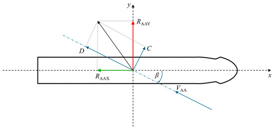
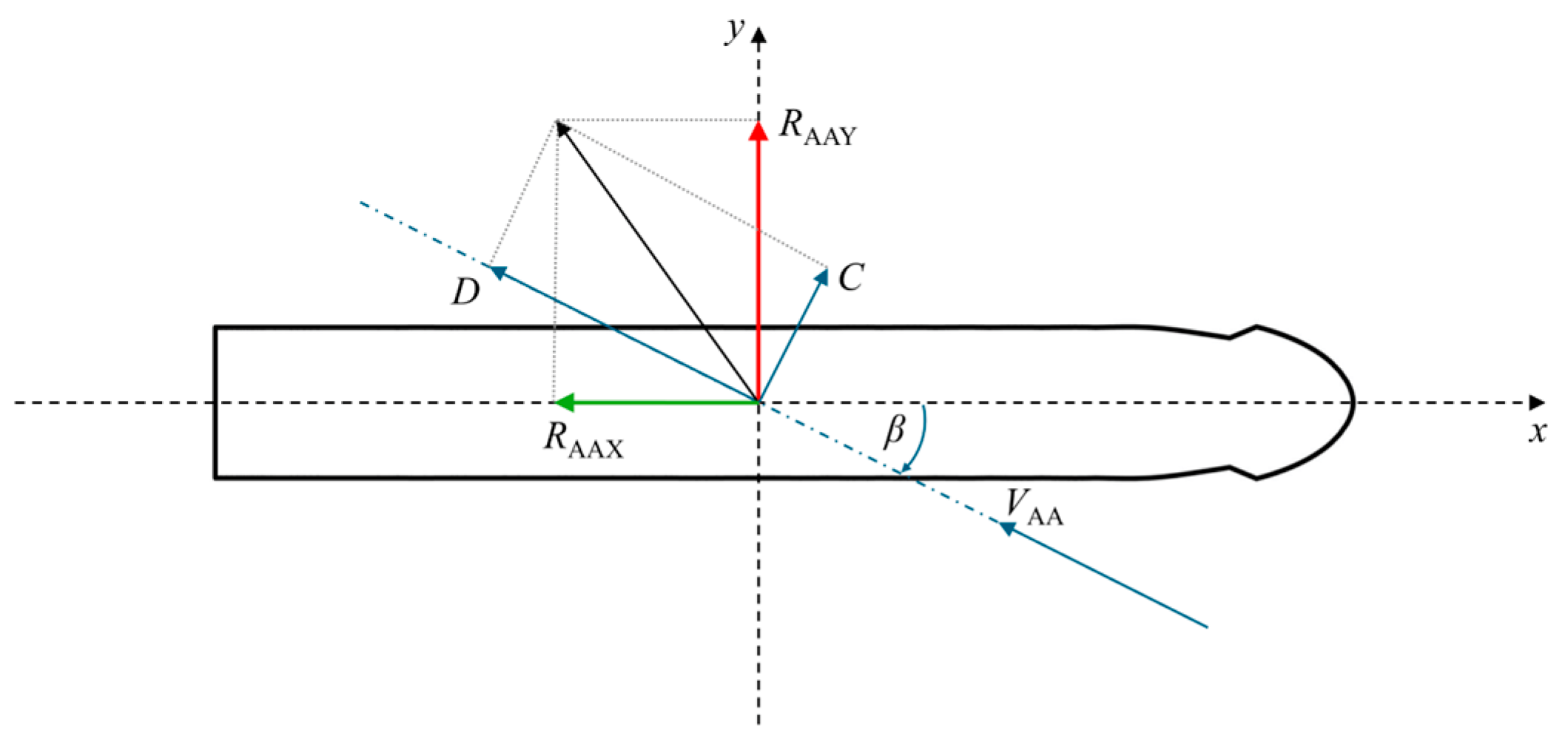
The wind load coefficients are calculated using the obtained forces from the CFD simulations. Figure 1 shows the coordinate system and the appropriate forces acting on the ship.

Figure 1. Schematic view of the forces acting on the ship.

According to the International Towing Tank Conference (ITTC) procedures [16] the wind load coefficients are calculated using the following functions:

$$C_X(\beta )={\displaystyle \frac{R_{AAX}(\beta )}{q_A{A}_F}}$$

(8)

$$C_Y(\beta )={\displaystyle \frac{R_{AAY}(\beta )}{q_A{A}_L}}$$

(9)

$$C_N(\beta )={\displaystyle \frac{M_z(\beta )}{q_A{A}_L{L}_{\mathrm{OA}}}}$$

(10)

where $\beta$ is the angle of attack, $A_L$ and $A_F$ are the lateral and transverse projected areas, respectively, $L_{\mathrm{OA}}$ is the length overall, $M_z$ is the yaw moment, and $q_A$ is the dynamic pressure calculated with the referent wind speeds depending on the component. More details for the referent wind speeds can be found in [16].

2.3. Empirical Methods

• Blendermann method

Blendermann [2] provided empirical expressions for the longitudinal and lateral force coefficients, as well as the yaw moment coefficient, formulated as functions of $\beta$, $A_F$, and $A_L$. From the wind tunnel measurements, the coefficients of the lateral ($C{D}_t$) and longitudinal ($C{D}_l$) resistance and cross-force parameter ($\delta$) are obtained. The longitudinal wind force coefficient $C_X$ is given with the following equation:

$$C_X={-CD}_{l{A}_F}{\displaystyle \frac{\cos \beta }{1-\frac{\delta }{2}\left(1-\frac{{CD}_l}{{CD}_t}\right){\mathrm{s}\mathrm{i}\mathrm{n}}^{2}2\beta }}$$

(11)

where $C{D}_{l{A}_F}$ is the coefficient of the longitudinal resistance expressed as $C{D}_{l{A}_F}=C{D}_l\cdot A_L/A_F$. Next, the lateral wind force coefficient $C_Y$ is equal to:

$$C_Y={CD}_t{\displaystyle \frac{\sin \beta }{1-\frac{\delta }{2}\left(1-\frac{{CD}_l}{{CD}_t}\right){\mathrm{s}\mathrm{i}\mathrm{n}}^{2}2\beta }}$$

(12)

And finally, the yaw moment coefficient $C_N$ is defined as follows:

$$C_N=\left[{\displaystyle \frac{s_L}{L_{\mathrm{OA}}}}-0.18\left(\beta -{\displaystyle \frac{\mathsf{\pi }}{2}}\right)\right]C_Y$$

(13)

In this study, the referent values for $C{D}_t$, $C{D}_l$, and $\delta$ are defined by the type of ship, which in this case is a loaded containership [2]. As such, the following values were taken:

$$C{D}_t=0.9$$

(14)

$$C{D}_{l{A}_F}=0.55$$

(15)

$$\delta =0.4$$

(16)

Isherwood method

The method provided by Isherwood [1] consists of three equations for the wind load coefficients that read as follows:

$$C_X=A_0+A_1{\displaystyle \frac{2A_L}{L_{\mathrm{OA}}^2}}+A_2{\displaystyle \frac{2A_F}{B^2}}+A_3{\displaystyle \frac{L_{\mathrm{OA}}}{B}}+A_4{\displaystyle \frac{S}{L_{\mathrm{OA}}}}+A_5{\displaystyle \frac{C}{L_{\mathrm{OA}}}}+A_{6}M$$

(17)

$$C_Y=B_0+B_1{\displaystyle \frac{2A_L}{L_{\mathrm{OA}}^2}}+B_2{\displaystyle \frac{2A_F}{B^2}}+B_3{\displaystyle \frac{L_{\mathrm{OA}}}{B}}+B_4{\displaystyle \frac{S}{L_{\mathrm{OA}}}}+B_5{\displaystyle \frac{C}{L_{\mathrm{OA}}}}+B_6{\displaystyle \frac{A_{\mathrm{SS}}}{A_L}}$$

(18)

$$C_N=C_0+C_1{\displaystyle \frac{2A_L}{L_{\mathrm{OA}}^2}}+C_2{\displaystyle \frac{2A_F}{B^2}}+C_3{\displaystyle \frac{L_{\mathrm{OA}}}{B}}+C_4{\displaystyle \frac{S}{L_{\mathrm{OA}}}}+C_5{\displaystyle \frac{C}{L_{\mathrm{OA}}}}$$

(19)

where $A_{\mathrm{SS}}$ is the lateral projected area of the superstructure, $B$ is the breadth, $S$ is the length of the perimeter of lateral projection of model excluding the waterline and slender bodies, $C$ is the distance between the bow and the centroid of the lateral projected area, and $M$ is the number of slender bodies (masts, kingposts, etc.). The constants $A_0$ to $A_6$, $B_0$ to $B_6$, and $C_0$ to $C_5$ are provided by Isherwood [1].

2.4. Numerical Setup

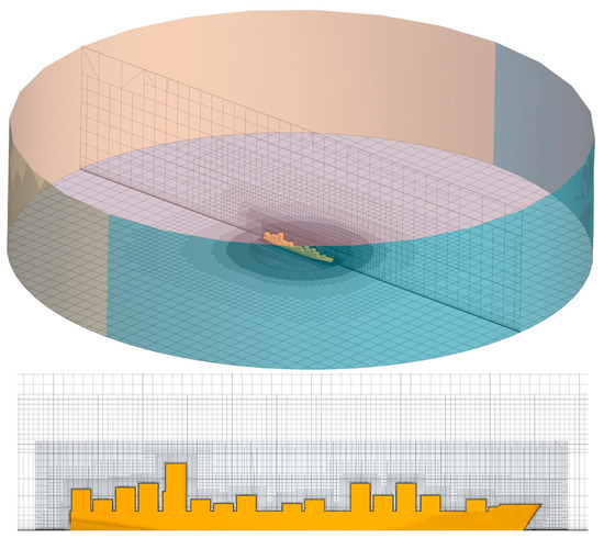
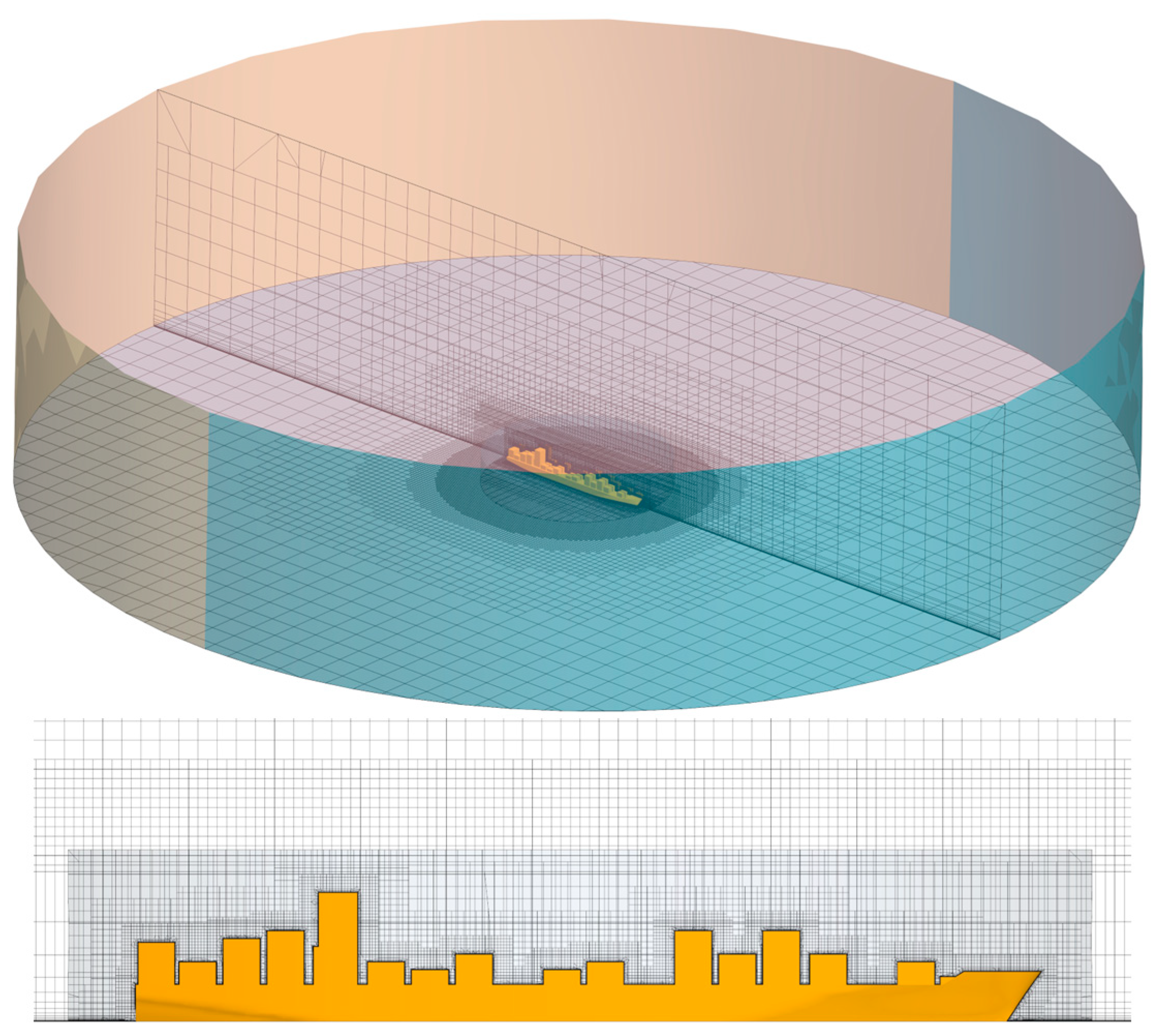
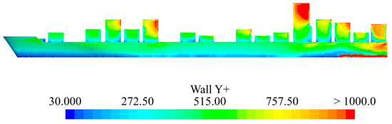
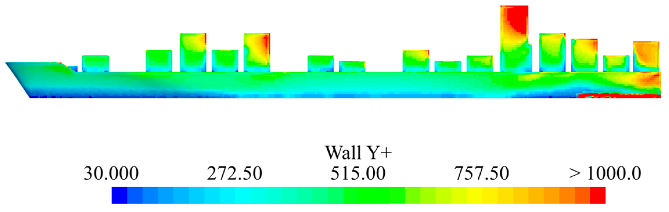
The computational domain around the full-scale containership consists of a fixed cylinder defining the boundaries of the domain and a rotating cylinder embedded, Figure 2. The reason for the rotating overset region is to obtain the wind loads on the ship for angles of attack in the range from 0° to 180° with 10° intervals in one simulation. The mesh consists of unstructured hexahedral cells, with local refinement applied near the ship. Additionally, mesh was refined through the generation of prism layers near the ship and container surfaces, ensuring that the non-dimensional wall distance $y^{+}$ exceeds 30, in accordance with the application of wall functions for boundary layer resolution. The distribution of $y^{+}$ values on the ship and container surfaces is presented in Figure 3 for a representative container configuration at the final time step. It can be observed that the minimum $y^{+}$ value of 30 is satisfied over all surfaces. The remaining container configurations exhibited similar distributions of $y^{+}$ values. The prism layers are enlarged to obtain a smooth transition from the boundary layer to the base mesh. Also, prism layers are created from the bottom boundary to follow the wind profile that is imposed at the inlet boundary. It is set up as a function of the height $z$ from the bottom surface as follows:

$$U(z)=U_{\mathrm{ref}}{\left({\displaystyle \frac{z}{z_{\mathrm{ref}}}}\right)}^{\alpha }$$

(20)

where $U_{\mathrm{ref}}=45 \mathrm{m}/\mathrm{s}$ and $z_{\mathrm{ref}}=10 \mathrm{m}$ are the referent velocity and height, respectively, and $\alpha =0.11$ is the velocity profile exponent. Along with the imposed wind profile, the turbulent dissipation rate and turbulent kinetic energy profiles are set at the inlet boundary as follows:

$$\epsilon (z)={\displaystyle \frac{(u^{*}{)}^3}{\kappa (z+z_0)}}$$

(21)

$$k(z)={\displaystyle \frac{(u^{*}{)}^2}{\sqrt{\left(C_{\mu }\right)}}}$$

(22)

where $\kappa =0.41$ is the von Karman constant, $z_0=0.0002$ is the aerodynamic roughness length [17], $C_{\mu }=0.09$ is the constant, and $u^{*}$ is the frictional velocity. On the bottom boundary, surface roughness is modelled using modified logarithmic-law wall functions, in which the roughness is represented through an equivalent sand-grain roughness defined by the following relation [18]:

$$k_s={\displaystyle \frac{9.793z_0}{C_s}}$$

(23)

where the roughness constant $C_s$ is equal to 1. More details on the imposed profiles at the inlet boundary and roughness on the bottom boundary are provided by Grlj et al. [8].

Figure 2. Computational domain and mesh details.

Figure 3. Distribution of $y^{+}$ values on the ship and container surfaces at the final time step.

2.5. Case Study

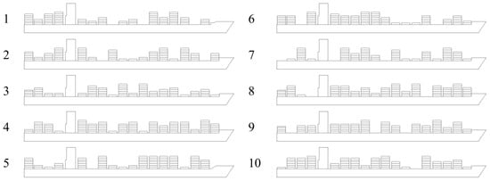
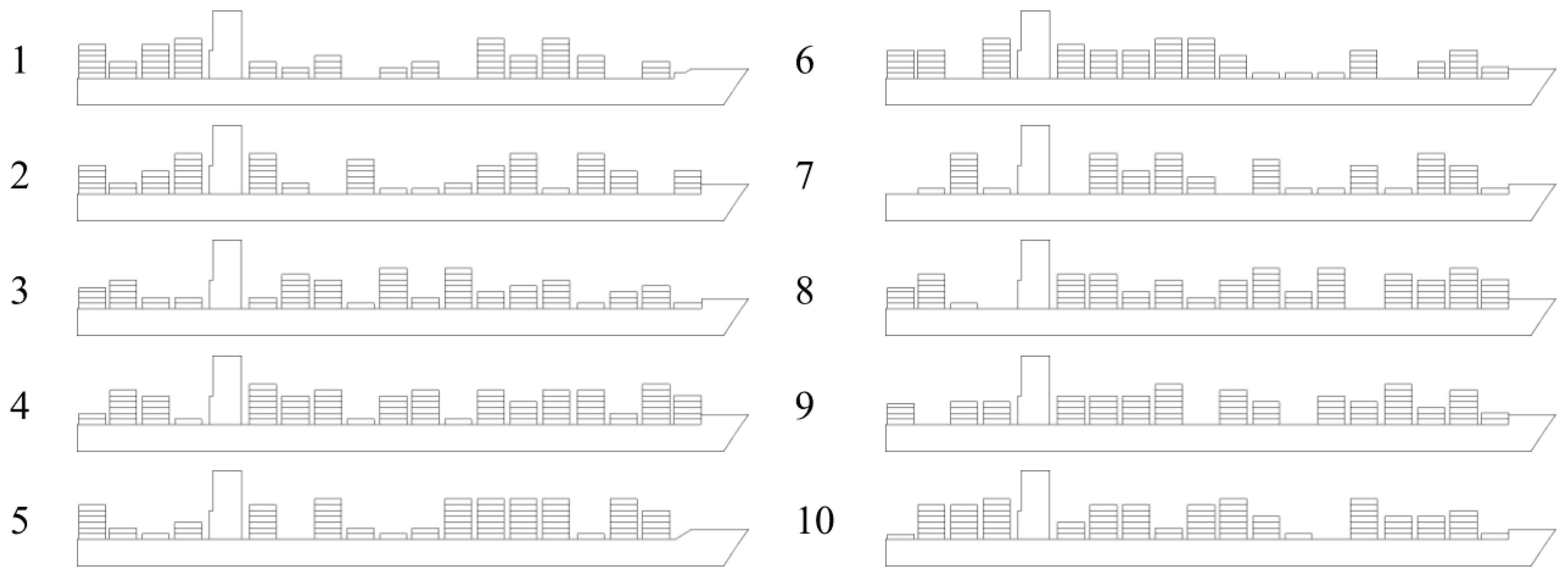
In this study the post-Panamax 6750 TEU containership is used [19,20]. Table 1 shows the main particulars and Figure 4 presents the side views of the containership loaded with random container configurations.

Table 1. Main particulars of the containership used in the study.

Main Particular	Value
$L_{\mathrm{OA}}$	303.98 m
$L_{\mathrm{WL}}$	292.48 m
$B$	40 m
$T$	11.98 m

Figure 4. Random container configurations.

As shown in Figure 4, the random container configurations are generated by varying the number of containers in each bay. The exact number of containers stacked in the 18 bays for each configuration is listed in Table 2. The mean lateral projected area is 6276.85 m², with a standard deviation of 224.72 m². The number of containers in each bay was limited to the maximum allowable stack height in accordance with the International Maritime Organization (IMO) Safety of Life at Sea regulations [21], which require the ship operator to maintain a forward line of sight from the bridge of at least 500 m or two ship lengths, whichever is smaller.

Table 2. Number of containers per bay for different container configurations.

Container Configuration	1	2	3	4	5	6	7	8	9	10
Bay
1	6	5	4	2	6	5	0	4	4	1
2	3	2	5	6	2	5	1	6	0	6
3	6	4	2	5	1	0	7	1	4	6
4	7	7	2	1	3	7	1	0	4	7
5	3	7	2	7	6	6	0	6	5	3
6	2	2	6	5	0	5	7	6	5	6
7	4	0	5	6	7	5	4	3	5	6
8	0	6	1	1	2	7	7	5	7	2
9	2	1	7	5	1	7	3	2	0	6
10	3	1	2	6	2	4	0	5	6	7
11	0	2	7	1	7	1	6	7	4	4
12	7	5	3	6	7	1	1	3	0	1
13	4	7	4	4	7	1	1	7	5	0
14	7	1	5	6	7	5	5	0	4	7
15	4	7	1	6	1	0	1	6	7	4
16	0	4	3	2	7	3	7	5	3	4
17	3	0	4	7	5	5	5	7	6	5
18	1	4	1	5	0	2	1	5	2	1

3. Results

Since the numerical results were previously verified and validated extensively by Grlj et al. [8], details of the verification study are omitted in this paper. The authors used the Grid Convergence Index (GCI) method for the assessment of the numerical uncertainty. The verification study was conducted with three grids using the same setup but with different numbers of cells and time steps. The reported GCI are consistently below 4% for both the $C_X$ and $C_Y$, with mostly oscillatory convergence obtained for most angles of attack. The calculated GCIs for the time step are lower in comparison to those obtained for the grid size.

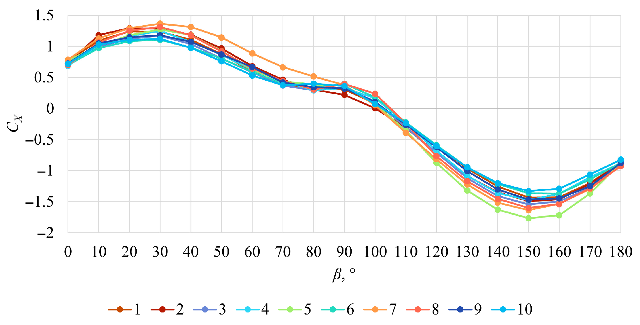
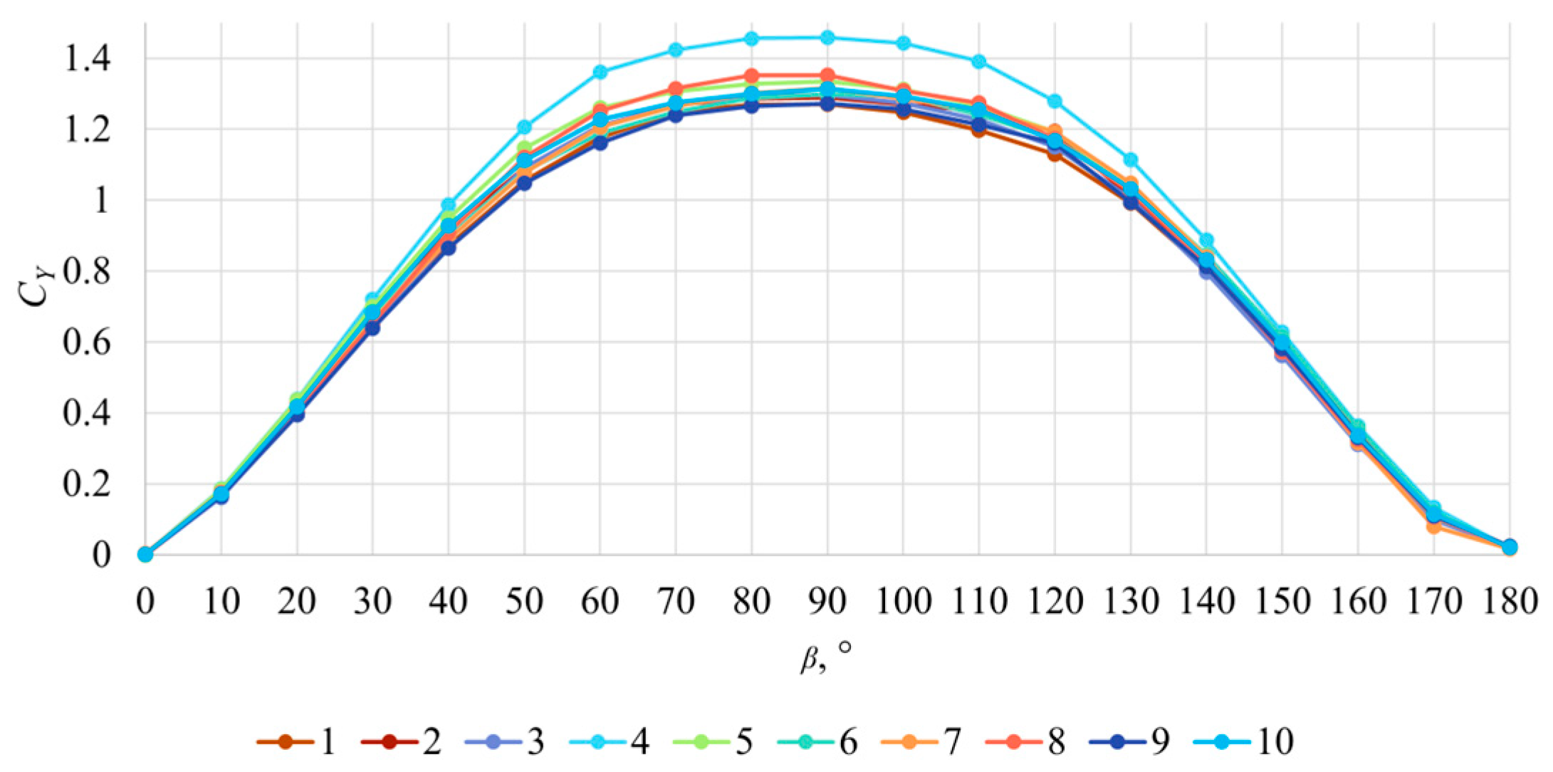
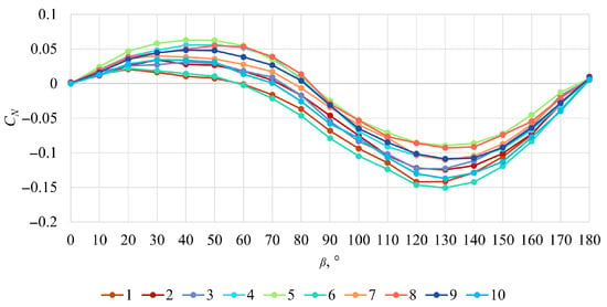
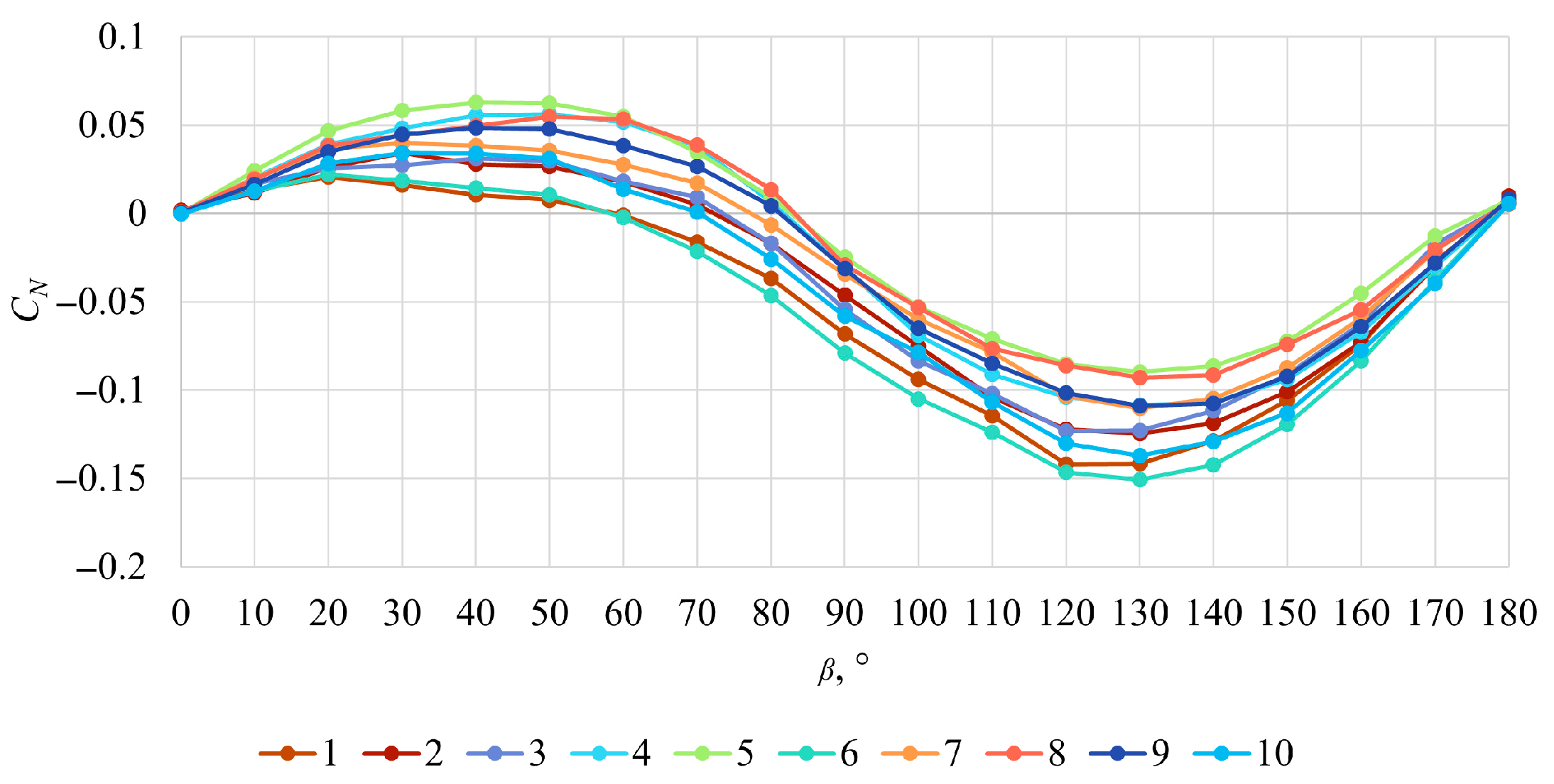
The wind load coefficients are calculated, and the obtained numerical results are shown in Figure 5, Figure 6 and Figure 7. Differences in the obtained $C_X$ are low, indicating that the different container configurations have only a minor influence on this coefficient. The highest absolute values are observed for container configuration 7 at angles of attack between 0° and 90°, and for container configuration 5 at higher angles of attack. The differences in the obtained $C_Y$ are somewhat more noticeable with the highest values obtained for container configuration 4 in the entire range of angles of attack. The lowest values are obtained for container configurations 2 and 9. Finally, the differences in the numerically obtained $C_N$ for different container configurations are more pronounced than those observed for $C_X$ and $C_Y$. The lowest values are obtained for container configuration 6, while the highest are obtained for container configuration 5. These discrepancies can be attributed to variations in container configurations. In particular, for $C_N$, higher container stacks positioned closer to the bow tend to produce higher values at lower angles of attack and lower absolute values at higher angles of attack. Conversely, when lower stacks are located nearer the bow, $C_N$ tends to be lower at smaller angles of attack.

Figure 5. Numerically obtained $C_X$ for each random container configuration.

Figure 6. Numerically obtained $C_Y$ for each random container configuration.

Figure 7. Numerically obtained $C_N$ for each random container configuration.

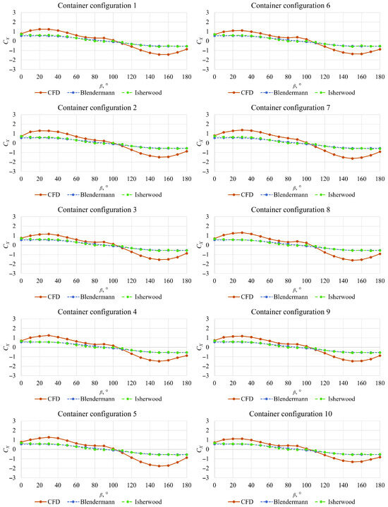
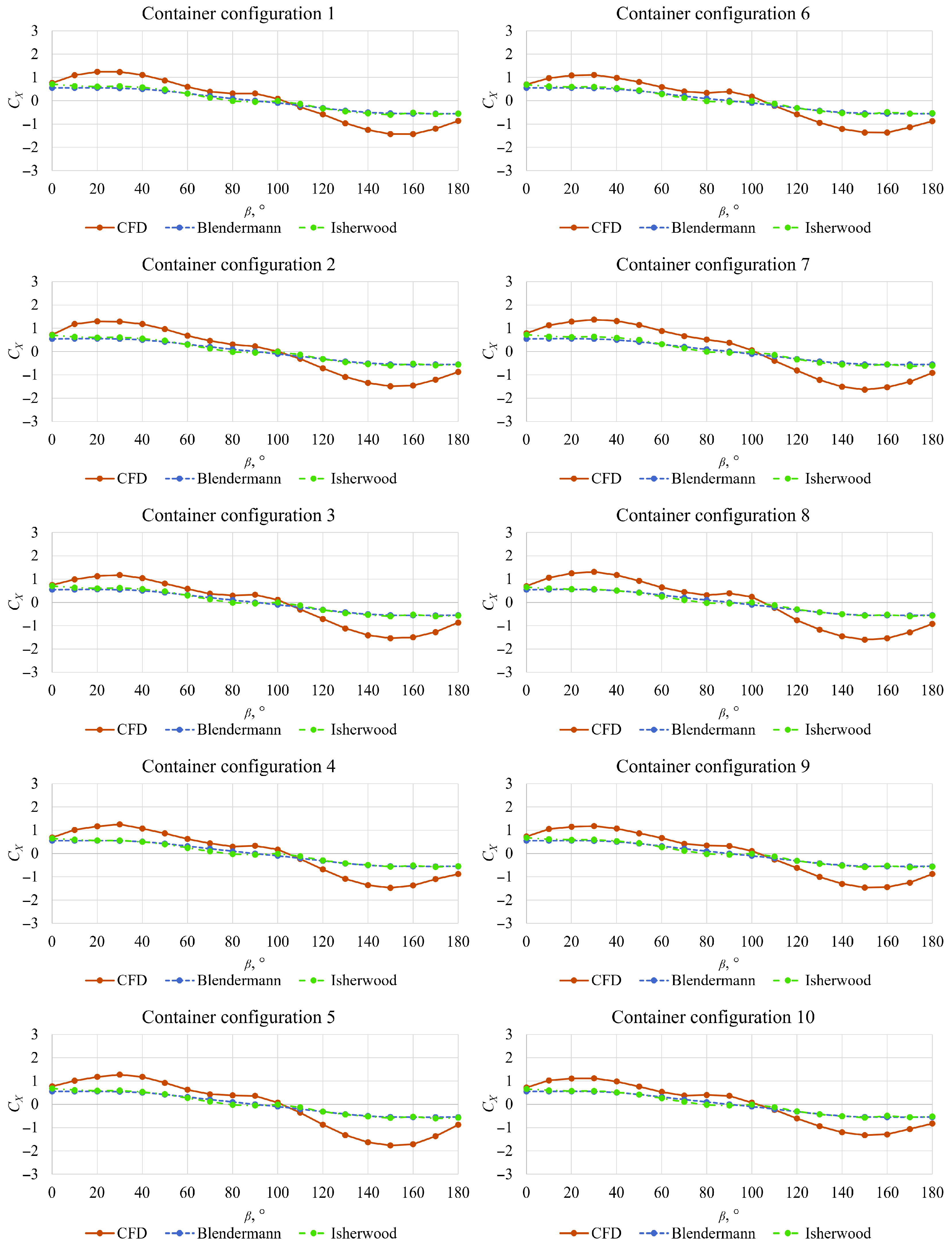
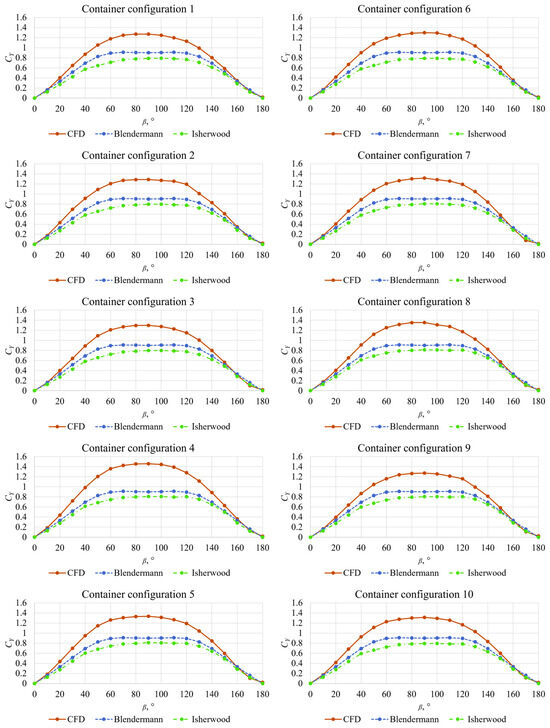
The numerically obtained wind load coefficients for each container configuration are compared to the coefficients obtained with the Blendermann and Isherwood methods in Figure 8, Figure 9 and Figure 10. The values obtained using empirical methods are in close agreement with each other. However, the absolute values of $C_X$ are lower than those predicted by the numerical simulations across the entire range of angles of attack for all considered container configurations. Both the Blendermann and Isherwood methods show the closest agreement with the numerical results at angles of attack between 60° and 120°, where $C_X$ approaches 0. At higher angles of attack, the discrepancies between the numerically and empirically obtained coefficients become more significant. For example, the relative deviations between the numerical results and those obtained using the Blendermann method reach up to 60% at an angle of attack of approximately 30°, and up to 68% at around 130°. Similar results are observed with the Isherwood method, where the relative deviations reach up to 55% at approximately 30° and 67% at around 130°. It should be noted that residual standard errors should be included with the wind load coefficients obtained with the Isherwood method. The residual standard errors depend on the angle of attack, and the mean values of the residual standard error are equal to 0.103 for $C_X$, 0.044 for $C_Y$, and 0.0127 for $C_N$ as reported by Isherwood [1].

Figure 8. Comparison between numerically and empirically obtained $C_X$.

Figure 9. Comparison between numerically and empirically obtained $C_Y$.

Figure 10. Comparison between numerically and empirically obtained $C_N$.

The numerically obtained $C_Y$ deviates substantially from the values predicted by the empirical methods. For all container configurations, the numerical values are higher than those calculated using the Isherwood and Blendermann methods. The largest discrepancies between the numerical results and those obtained using the Isherwood method are approximately 40%, while those for the Blendermann method are slightly lower, at around 30%. This finding is consistent with the results reported by Prpić-Oršić et al. [10], who demonstrated that wind tunnel wall effects have significant influence on measured wind load coefficients. In the present study, blockage effects are deliberately neglected to highlight their impact on the results. This approach underscores a key advantage of CFD, as open-water conditions can be simulated without requiring corrections for blockage effects. Another source of discrepancies between the numerically predicted wind loads and those obtained using empirical methods may be attributed to free-surface effects regarding the wave patterns generated by the ship, as well as potential scale effects. The results obtained using the Blendermann and Isherwood methods are in close agreement with each other, with Blendermann generally yielding slightly higher values than Isherwood. It should also be noted that the $C_Y$ predicted by Blendermann method is identical for all container configurations, as it does not depend on the projected areas. The differences in predicted $C_Y$ by the Isherwood method for the various container configurations are small but not negligible.

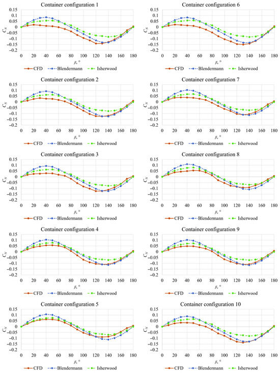
Finally, Figure 10 presents a comparison between the numerically obtained $C_N$ and coefficients obtained with empirical methods. The numerical simulations yield lower values of $C_N$ than those predicted by the empirical methods for all container configurations. The discrepancies are particularly pronounced for container configurations 1 and 6. The Blendermann method predicts higher absolute values of $C_N$ compared to the Isherwood method at angles of attack between 20° and 60°, as well as between 100° and 160°. At angles of attack from 130° to 180° the coefficients obtained with Blendermann method are in close agreement with those obtained numerically for all container configurations.

At these angles of attack, the $C_N$ values approach zero, and the relative deviations between the numerical results and those obtained using the Blendermann method reach up to approximately 30%, depending on the container configuration. Overall, the CFD simulations indicate larger variations in $C_N$ among different container configurations than those captured by the empirical methods.

4. Conclusions

This study presents a numerical assessment of wind loads acting on a post-Panamax 6750 TEU containership loaded with random container configurations. Full-scale simulations were carried out under open-sea conditions using the Reynolds-averaged Navier–Stokes equations with the Realizable k-ε two-layer turbulence model, and the resulting aerodynamic forces and moments were expressed in terms of non-dimensional wind load coefficients in accordance with ITTC recommendations. The numerical results were compared with two widely used empirical methods, namely those proposed by Isherwood [1] and Blendermann [2].

The results demonstrate that random container configurations can lead to noticeable variations in all wind load coefficients, with the most pronounced differences observed in the yaw moment coefficient. While variations in the longitudinal wind load coefficient were relatively small, both the lateral wind load and yaw moment coefficients exhibited a stronger sensitivity to container arrangement, highlighting the importance of accounting for realistic loading conditions when estimating wind loads on large containerships.

Comparison with empirical methods indicates that the smallest discrepancies relative to the numerical results occur for the longitudinal wind load coefficient. In contrast, significant deviations are observed for the lateral wind load coefficient, for which CFD simulations consistently predict higher values compared to those obtained with empirical methods. These differences are primarily attributed to the fact that the empirical methods are based on wind tunnel experiments affected by blockage effects, whereas the present CFD simulations represent open-water conditions. Among all coefficients, the yaw moment exhibits the largest variations across different container configurations, as captured by all methods.

This study provides insights into the limitations of existing empirical approaches and demonstrates the advantage of using CFD for improved wind load prediction in ship design and operational performance assessments. In addition to the aforementioned limitations of the empirical methods, it should be noted that both the Isherwood and Blendermann methods were developed based on conventional ship geometries. Consequently, a reduction in accuracy can be expected when these methods are applied to modern containerships, particularly ultra-large containerships, mainly due to their larger sizes.

References

- Isherwood, R.M. Wind Resistance of Merchant Ships. Trans. R. Inst. Nav. Archit. 1973, 115, 327–338. [Google Scholar]
- Blendermann, W. Parameter Identification of Wind Loads on Ships. J. Wind. Eng. Ind. Aerodyn. 1994, 51, 339–351. [Google Scholar] [CrossRef] [Scilit]
- Andersen, I.M.V. Wind Loads on Post-Panamax Container Ship. Ocean Eng. 2013, 58, 115–134. [Google Scholar] [CrossRef] [Scilit]
- Janssen, W.D.; Blocken, B.; van Wijhe, H.J. CFD Simulations of Wind Loads on a Container Ship: Validation and Impact of Geometrical Simplifications. J. Wind. Eng. Ind. Aerodyn. 2017, 166, 106–116. [Google Scholar] [CrossRef] [Scilit]
- He, N.; Mizutani, K.; Ikeda, Y. Reducing Air Resistance Acting on a Ship by Using Interaction Effects between the Hull and Accommodation. Ocean Eng. 2016, 111, 414–423. [Google Scholar] [CrossRef] [Scilit]
- Nguyen, T.V.; Shimizu, N.; Kinugawa, A.; Tai, Y.; Ikeda, Y. Numerical Studies on Air Resistance Reduction Methods for a Large Container Ship with Fully Loaded Deck-Containers in Oblique Winds. In Proceedings of the VII International Conference on Computational Methods in Marine Engineering (MARINE 2017), Nantes, France, 15–17 May 2017. [Google Scholar]
- Wnęk, A.D.; Guedes Soares, C. CFD Assessment of the Wind Loads on an LNG Carrier and Floating Platform Models. Ocean Eng. 2015, 97, 30–36. [Google Scholar] [CrossRef] [Scilit]
- Grlj, C.G.; Degiuli, N.; Tuković, Ž.; Farkas, A.; Martić, I. The Effect of Loading Conditions and Ship Speed on the Wind and Air Resistance of a Containership. Ocean Eng. 2023, 273, 113991. [Google Scholar] [CrossRef] [Scilit]
- Degiuli, N.; Grlj, C.G.; Martić, I.; Šegota, S.B.; Anđelić, N.; Majnarić, D. Machine Learning Models for the Prediction of Wind Loads on Containerships. J. Mar. Sci. Eng. 2025, 13, 417. [Google Scholar] [CrossRef] [Scilit]
- Prpić-Oršić, J.; Valčić, M.; Čarija, Z. A Hybrid Wind Load Estimation Method for Container Ship Based on Computational Fluid Dynamics and Neural Networks. J. Mar. Sci. Eng. 2020, 8, 539. [Google Scholar] [CrossRef] [Scilit]
- Wang, G.; Feng, Y.; Dai, Y.; Chen, Z.; Wu, Y. An Efficient Prediction Method for Wind Loads on Container Ships Based on Numerical Simulation and Gaussian Process Regression. Ocean Eng. 2026, 343, 123384. [Google Scholar] [CrossRef] [Scilit]
- Grlj, C.G.; Degiuli, N.; Martić, I. Experimental and Numerical Assessment of the Effect of Speed and Loading Conditions on the Nominal Wake of a Containership. Brodogradnja 2024, 75, 75405. [Google Scholar] [CrossRef] [Scilit]
- Ma, Z.X.; Li, N.; Zeng, Q.; Deng, X.B.; Shi, C. Influence of Scale Effect on Flow Field Offset for Ships in Confined Waters. Brodogradnja 2024, 75, 75106. [Google Scholar] [CrossRef] [Scilit]
- Farkas, A.; Degiuli, N.; Martić, I. Numerical simulation of viscous flow around a tanker model. Brodogradnja 2017, 68, 109–125. [Google Scholar] [CrossRef] [Scilit]
- Romani, S.; Morgut, M.; Parussini, L.; Piller, M. Uncertainty Quantification and Global Sensitivity Analysis of Turbulence Model Closure Coefficients for Sheet Cavity Flow around a Hydrofoil. Brodogradnja 2025, 76, 76105. [Google Scholar] [CrossRef] [Scilit]
- ITTC. Guideline on the CFD-Based Determination of Wind Resistance Coefficients, 7.5-03-02-05. In ITTC-Recommended Procedures and Guidelines; ITTC: Hobart, Australia, 2024. [Google Scholar]
- Wieringa, J. Updating the Davenport roughness classification. J. Wind. Eng. Ind. Aerodyn. 1992, 41, 357–368. [Google Scholar] [CrossRef] [Scilit]
- Ricci, A.; Janssen, W.D.; van Wijhe, H.J.; Blocken, B. CFD simulation of wind forces on ships in ports: Case study for the Rotterdam Cruise Terminal. J. Wind. Eng. Ind. Aerodyn. 2020, 205, 104315. [Google Scholar] [CrossRef] [Scilit]
- Kim, Y.; Kim, J.H. Benchmark Study on Motions and Loads of a 6750-TEU Containership. Ocean Eng. 2016, 119, 262–273. [Google Scholar] [CrossRef] [Scilit]
- Degiuli, N.; Martić, I.; Pedišić Buča, M.; Grlj, C.G. Benchmark study on resistance and propulsion characteristics of a 6750-TEU container ship. Ocean Eng. 2025, 319, 120300. [Google Scholar] [CrossRef] [Scilit]
- International Maritime Organization. SOLAS: Consolidated Edition 2001; International Maritime Organization: London, UK, 2001. [Google Scholar]
Disclaimer/Publisher’s Note: The statements, opinions and data contained in all publications are solely those of the individual author(s) and contributor(s) and not of MDPI and/or the editor(s). MDPI and/or the editor(s) disclaim responsibility for any injury to people or property resulting from any ideas, methods, instructions or products referred to in the content. |
© 2026 by the authors. Licensee MDPI, Basel, Switzerland. This article is an open access article distributed under the terms and conditions of the Creative Commons Attribution (CC BY) license.