


Abstract
Visual perception in Unmanned Surface Vehicles (USVs) suffers from drastic lighting changes and missing texture features. These factors lead to depth scale drift and motion estimation bias. Moreover, existing multi-modal fusion models are computationally complex and unfit for resource-limited edge devices. To address these problems, a lightweight Radar–Vision Fusion (Geo-RVF) algorithm is proposed. To supplement spatial information, point clouds are projected to build sparse depth maps. A probability consistency-based depth correction module is designed to suppress water noise. This helps extract accurate geometric anchors to guide visual depth propagation. Subsequently, a Recurrent Autoregressive Network (RAN) fuses radar and image features in the temporal dimension. This resolves dynamic positional deviations caused by texture degradation and distant small targets. After real-time optimization, Geo-RVF achieves 23 FPS on the Jetson Orin NX. On a collected dataset, the method attains a mean average precision (mAP) 50–90 of 44.2% and a mean intersection over union (mIoU) of 99%, outperforming HybridNets and Achelous.
1. Introduction
Unmanned Surface Vehicles (USVs) play an increasingly important role in marine research and resource management [1]. For USV autonomous navigation, environmental perception is the prerequisite for obstacle avoidance and path planning. Visual perception is currently the primary method due to its high resolution, rich semantics, and low cost. To facilitate 3D motion control, 2D images are typically converted into a Bird’s-Eye View (BEV). BEV eliminates perspective effects and provides a unified spatial scale. However, constructing the BEV space relies heavily on precise depth estimation, which remains a major challenge for visual sensors in complex water environments.
Although images contain rich semantics, they lack absolute physical scale constraints when mapped to BEV. This leads to severe depth scale problems. In dynamic water scenes (characterized by strong reflections, waves, and textureless areas), depth estimation models often degrade, causing significant scale drift. Furthermore, pure vision has limitations in dynamic perception. Inferring speed from multi-frame analysis is computationally slow and easily affected by hull vibration. Due to missing depth information and uncertain motion estimation, pure vision cannot meet USV safety requirements. Therefore, sensors with physical ranging capabilities must be introduced.
Sensor fusion must balance performance, hardware cost, and computational efficiency. LiDAR provides dense point clouds but is too expensive and power-hungry for small USVs. In contrast, millimeter-wave radar works effectively in all weather conditions, penetrating rain and fog [2]. Although its point clouds are sparse, it provides Doppler velocity, which complements high-resolution visual semantics. Therefore, combining cameras with radar is the most practical choice for USVs [3].
Deep learning has significantly advanced multi-modal fusion, particularly in the automotive autonomous driving sector. However, transferring these mainstream solutions directly to USVs presents a critical bottleneck. Although methods like Centerfusion [4] attempt to improve 3D perception by associating radar with visual center points, they still struggle to construct a unified and dense representation. Conversely, state-of-the-art Transformer-based detectors [5] and BEV frameworks [6] offer comprehensive fusion but rely on complex feature interactions. While highly accurate, they demand massive memory and computational resources. Such hardware is readily available in automobiles but is strictly prohibited on small USVs, which operate under severe payload and battery constraints using low-power edge computing platforms. Furthermore, although pure 2D visual detectors operate extremely fast, they lack functions such as depth estimation, radar fusion, and 3D BEV transformation, and therefore cannot meet the requirements for safe unmanned surface vessel navigation. Consequently, there is an urgent, unmet need for a perception system that can achieve the robustness of 3D BEV fusion while strictly adhering to the computational limitations of USV edge devices. To address this gap, we propose Geo-RVF, a lightweight perception system for edge devices. By compressing a complete multi-modal 3D BEV pipeline into just 10.3 GFLOPs, our approach bridges the gap between functionally limited pure vision models and computationally prohibitive multi-modal frameworks, achieving a truly lightweight status for edge devices. Our algorithm uses radar point clouds as reliable geometric priors and dynamically corrects visual depth and velocity deviations, ensuring 3D precision with reduced computational overhead.
To implement this, Geo-RVF establishes a pipeline from depth inference to state correction. The key is fusing camera and radar data to generate spatially accurate BEV features. We designed a depth correction module based on probability consistency. This maps radar points as sparse “geometric anchors” to guide visual depth scaling. Subsequently, a Recurrent Autoregressive Network (RAN) fuses radar Doppler velocity with visual features. This addresses position deviations caused by distant small targets or texture degradation. Finally, the system is optimized for the Jetson Orin NX, achieving high-precision real-time perception.
The contributions of this study are as follows:
- A lightweight radar-vision fusion architecture for edge devices. Based on Lift, Splat, Shoot (LSS) [7] and YOLO-AFM (YOLO with Adaptive Feature Module) [8], we incorporate radar point clouds. By combining early geometric priors with late constraints, we enhance perception robustness in complex lighting environments.
- A depth scale correction mechanism based on radar geometric anchors. This overcomes the scale drift of monocular depth estimation. It uses radar as a physical constraint, combining adaptive matching and spatial weight transfer for accurate BEV mapping.
- A motion modeling and tracking method. We introduce a RAN to model temporal states and use an Extended Kalman Filter (EKF) to fuse radar information. This strategy effectively alleviates the lag and jitter found in pure visual speed estimation.
2. Related Work
2.1. Radar–Camera Fusion for Object Detection
Due to the complementary nature of radar and cameras, fusing these sensors is a mainstream solution for 3D object detection. Existing methods generally fall into two categories: Region of Interest (ROI)-based fusion and end-to-end fusion.
ROI-based fusion typically generates proposals from one modality and refines them with features from the other. Early methods projected radar points onto the image plane to generate candidate regions [9]. However, projection discards the depth dimension, leading to a loss of 3D spatial information [10]. To address radar sparsity, recent studies generate proposals from images first. Centerfusion [4] is a representative method. It uses pillar expansion to address the lack of radar height information and associates radar detections with image frustums to regress velocity and depth. Similarly, CRAFT [11] proposes a soft association mechanism in the polar coordinate system. It uses consecutive cross-attention layers to adaptively exchange spatial context, handling spatial misalignment between sensors.
End-to-end methods integrate features from both modalities into a unified framework. This enables comprehensive feature interaction. Methods based on 3D proposal prediction incorporate a radar processing branch into the detection framework. Li et al. [12] addressed hull shaking deviations using motion-compensated projection and distance association modules, achieving 50.1% AP. FMA-FCOS [13] improves detection performance in adverse weather and occlusion via radar feature enhancement, gated fusion, and adaptive feature pyramids. Additionally, Hwang et al. [14] focused on robust detection of distant small objects in adverse weather for autonomous driving. They proposed spatial partition projection and weighted fusion modules. With the rise of BEV perception, transforming image features into a unified BEV space for fusion has become a mainstream approach. RCM-Fusion [15] is built on the BEVFormer [16] architecture and uses radar positions to construct optimized queries. Xu et al. [17] proposed RCFusionNet with a radar-guided two-stage fusion strategy. It enhances robustness by interacting with radar data during BEV feature generation and fusion.
2.2. Depth Estimation
2.2.1. Monocular Depth Estimation
In recent years, monocular depth estimation has widely adopted deep learning. Mainstream works formulate the problem as pixel depth regression [18,19] or depth distribution classification [20]. Early works treated depth estimation as a regression problem, using LiDAR depth labels as supervision for training on large-scale datasets. Eigen et al. [21] proposed a multi-scale CNN that first regresses a coarse depth map and then refines it. Subsequently, fully convolutional networks (FCNs) and U-Net became standard architectures [22,23]. They use skip connections to recover spatial resolution lost during downsampling. Although accurate, these supervised methods face severe generalization issues [24]. Models trained on specific datasets (e.g., NYUv2, KITTI) struggle to estimate depth in unseen scenes.
To reduce reliance on ground truth data, self-supervised learning has become a major research direction. These methods treat depth estimation as an image synthesis problem, optimizing via reprojection loss [25]. Methods proposed by Garg et al. [26] and Godard et al. [27] use rectified stereo supervision. They estimate disparity via left-right consistency loss and convert it to depth. While effective, stereo-based training requires synchronized stereo cameras, limiting data availability. Zhou et al. [25] proposed a framework to learn depth and ego-motion from monocular video sequences using a pose network. Monodepth2 [28] significantly improved baselines by introducing minimum reprojection loss for occlusion and masking strategies for moving objects. However, monocular video methods suffer from scale ambiguity and sensitivity to dynamic objects [29].
Although these methods achieve high performance on public benchmarks, generalizing to diverse environments remains a key challenge. Consequently, generative adversarial networks (GANs) are increasingly used to align synthesized and real feature distributions [30]. Recent research also explores online learning and meta-learning to adapt pre-trained models to new scenes during inference [31], addressing generalization issues in real-world applications.
2.2.2. Point Cloud–Vision Depth Estimation
Monocular depth estimation excels at recovering scene structure but lacks metric scale. To recover precise metric depth, integrating active range sensors (e.g., LiDAR or radar) is promising. Existing methods generally fall into two categories: dense LiDAR-based depth completion and sparse radar–camera fusion.
Mainstream depth completion projects LiDAR points onto the image plane to create sparse depth maps, which are then completed by encoder–decoder networks [32]. While feasible, this discards inherent 3D geometric information. To preserve 3D geometry, recent studies extract features directly from 3D space before fusion. For instance, point-based branches [33] or GNN [34] propagate features in 3D space. However, these methods rely on high-quality, dense LiDAR data and struggle with extremely sparse radar data.
Compared to LiDAR, millimeter-wave radar is cheaper and more robust in harsh environments. Early methods, such as that proposed by Lin et al. [35], directly projected radar points, resulting in sparse and blurry images. To address this, techniques like DORN [36] expand radar points into pillars or use ordinal regression to model depth distribution. Since radar echoes contain noise, simple fusion often leads to artifacts. Recent research focuses on learning reliable associations between radar points and image pixels. Long et al. [37] use Doppler velocity and optical flow to filter dynamic outliers. Instead of hard projection, Singh et al. [38] propose confidence scores for radar–pixel correspondence to generate semi-dense depth maps, followed by a gated fusion network.
Architectures combining multi-modal features have also evolved. Traditional methods simply concatenate radar and image features [39]. However, directly fusing heterogeneous data can confuse the learning process, causing aliasing artifacts and blurred boundaries [40]. An emerging trend separates shape prediction from scale recovery. Methods like RadarCam-Depth [41] use image branches to predict high-fidelity, scale-free depth maps and use radar data solely to learn metric scales. Similarly, GET-UP [42] introduces a point cloud upsampling module [43] to densify radar points based on visual features, enhancing geometric consistency. These methods demonstrate that preserving the unique characteristics of each modality improves performance. However, none of the above methods account for radar detection errors, leading to suboptimal depth estimation accuracy.
3. Methods
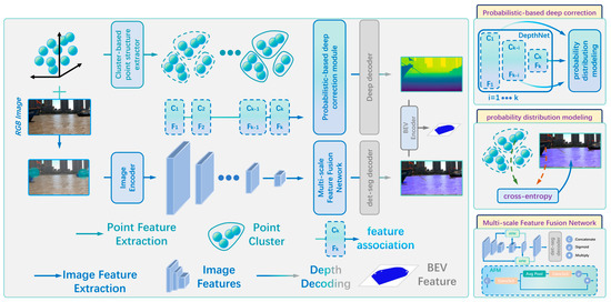
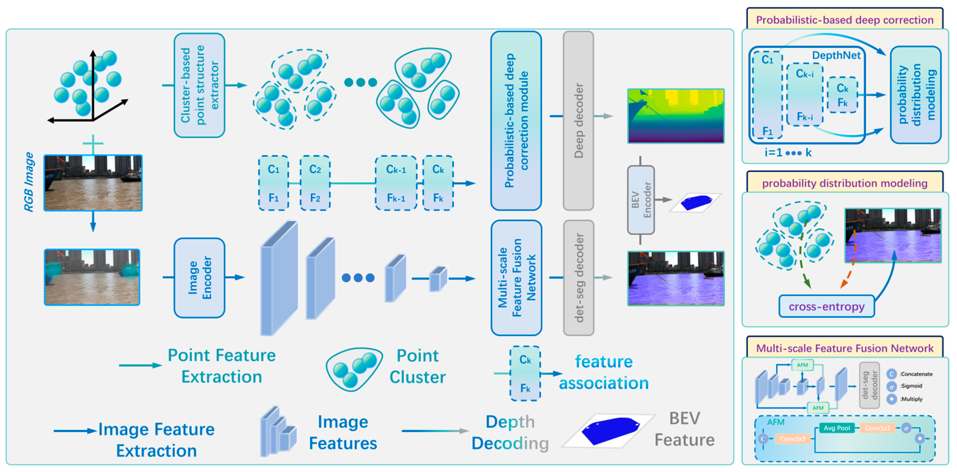
As illustrated in Figure 1, the proposed Geo-RVF framework operates as an end-to-end Multi-Task Learning (MTL) system, taking images, radar point clouds, and calibration parameters as inputs. First, the camera image is fed into a shared visual backbone (an improved CSPDarknet) to extract multi-scale hierarchical features. To minimize computational redundancy, these shared features then branch into three parallel task heads: (1) a 2D Object Detection head, (2) a Drivable Area Segmentation head, and (3) a Depth Estimation head.
Figure 1.
Overall framework of the perception algorithm. The system takes images and radar point clouds as inputs. A backbone network generates 2D detection, segmentation, and depth features in parallel. Radar point clouds are used as geometric anchors to probabilistically correct visual depth. The final output is a Bird’-Eye View (BEV) image.
Simultaneously, sparse radar point clouds are processed and clustered. During the depth inference stage, target-associated radar point clouds serve as spatial geometric anchors to constrain and correct the visual depth probabilities. Subsequently, the fused multi-modal features are transformed into the unified BEV space using the LSS paradigm. Finally, a RAN module is constructed to jointly model target appearance and temporal motion states, and an Extended Kalman Filter (EKF) is employed to fuse radar radial Doppler velocity with visual displacement vectors.
3.1. Geometrically Consistent Depth Estimation
3.1.1. Visual Discrete Depth Estimation
Based on semantic features from the multi-scale fusion network, the depth branch recovers dense depth information on the image plane. Since the fused features integrate radar spatial hints and camera semantics, the depth network can more sharply capture distance differences between target contours and the background. In the depth estimation branch, fused features are fed into a depth network encoder. This module extracts distance-sensitive features through convolutional layers, reduces channel redundancy, and outputs a single-channel depth map via a 1 × 1 convolutional head. A Sigmoid function then constrains the output to a normalized interval, mapping it to the depth range of interest :
Although this method incorporates radar features, relying solely on convolutional networks remains a visual depth estimation task. It is prone to scale drift in open waters. Therefore, this output serves only as an initial estimate. It requires correction in the next stage using radar physical measurements as geometric anchors.
3.1.2. Visual Depth Estimation Correction
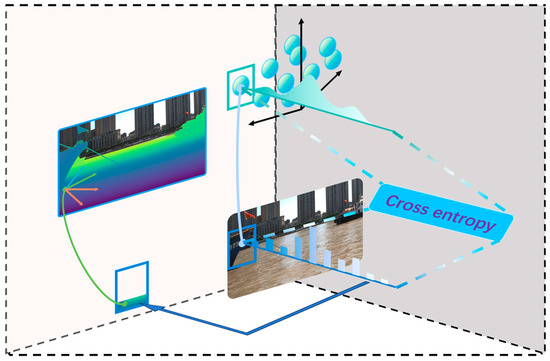
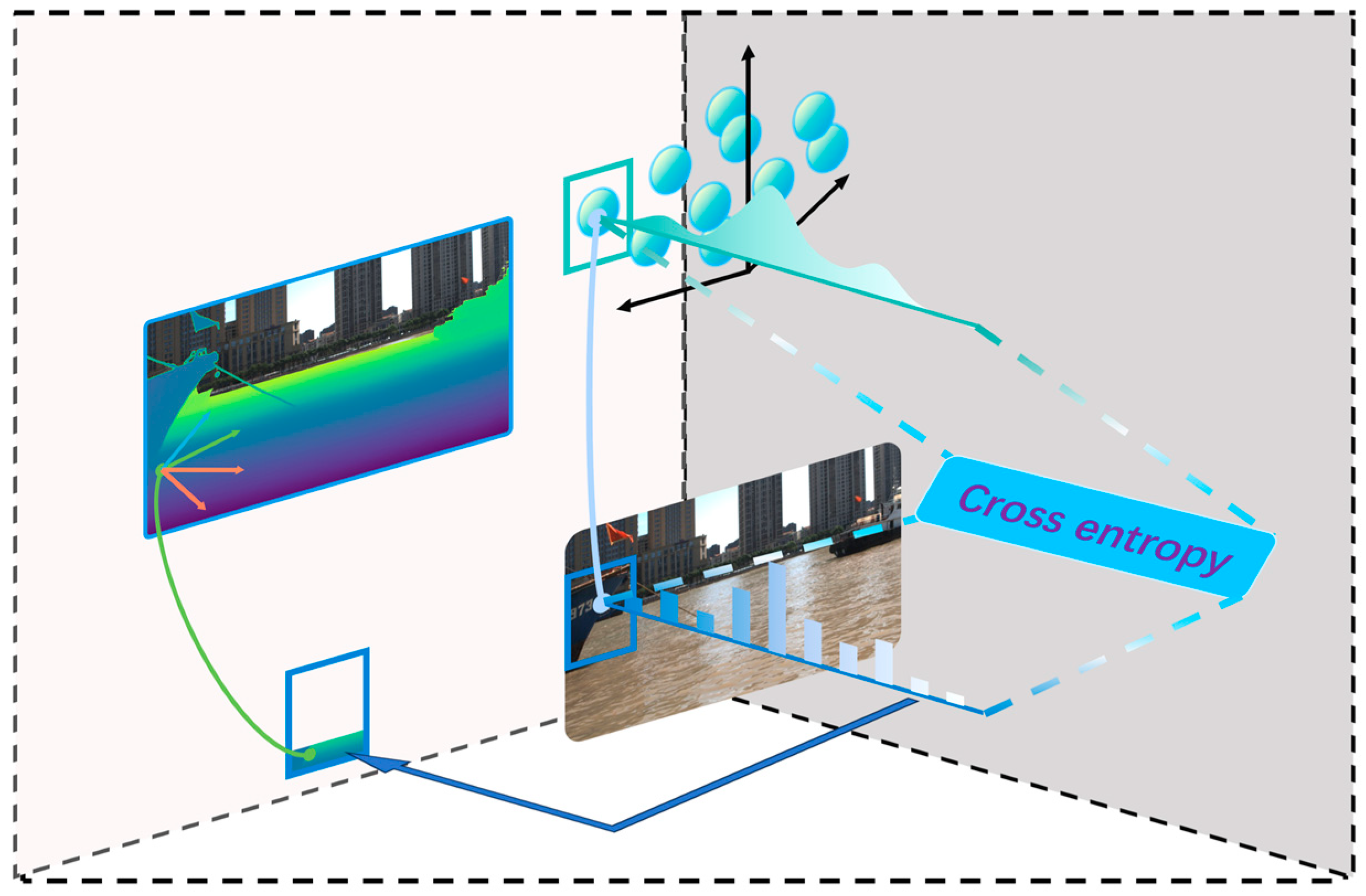
To recover precise distance scale, inspired by LSS probabilistic concepts, we designed a depth correction mechanism based on radar geometric anchors, as illustrated in Figure 2. It does not forcibly overwrite visual predictions. Instead, it optimizes depth estimation by matching probability distributions. For successfully associated radar targets, the radar measurement is not perfectly accurate. Measurements are affected by hull swaying and target pose changes. Therefore, the system models it as a Gaussian probability distribution along the optical ray:
where the variance is adaptively adjusted based on target distance and association confidence. This constructs a sparse but reliable depth probability distribution.
Figure 2.
Illustration of Radar Depth Probabilistic Modeling and Correction.
In water scenes, the actual scale of objects is primarily manifested through the waterline contact. To effectively propagate radar scale information to unmatched visual depths, the algorithm focuses on the contact region of each target. During training, the depth value regressed by the visual network is also converted into a probability distribution . We minimize cross-entropy to align the visual depth distribution with the radar distribution:
By minimizing this loss, radar physical scale information is incorporated as a soft constraint into the depth regression network. Leveraging the LSS paradigm, the network preserves detailed features when visual textures are clear. When scale drift occurs, radar anchors pull the depth prediction back to the correct range. This achieves a geometrically unified BEV construction.
3.1.3. Multi-Task Joint Loss Optimization
To avoid any single task dominating the entire learning process, we dynamically balance the multi-task loss by adopting homoscedastic task uncertainty [44]. The overall loss function is redefined as:
where represents the loss value for each specific task (detection, segmentation, initial visual depth, and radar-guided scale correction). For each task, we introduce , which is a learnable logarithmic variance parameter. To ensure stability during the early training stage, all are initialized to 0.
This formulation ensures that no single task dominates the entire network. The dynamic weights for each task are actually . During backpropagation, if the loss value of a specific task is significantly large, the network will adaptively learn a larger variance to minimize the overall objective. This exponentially increasing denominator significantly reduces the effective weight of that task, thereby preventing its gradient from disrupting the shared multi-scale features. Meanwhile, the additive term 1/2 serves as a regularization penalty to prevent the network from simply minimizing the loss by infinitely increasing . As we confirmed by our training metrics, this self-regulating mechanism can standardize the gradient scale and enable all parallel tasks to reach consensus harmoniously.
3.2. Radar–Visual Fusion Object Tracking
3.2.1. Object Detection
Radar and LiDAR share similar data forms but differ significantly in resolution and precision. Therefore, directly transferring state-of-the-art LiDAR architectures is difficult. We adopt a multi-stage hybrid fusion strategy to handle radar sparsity and noise effectively. To overcome sparsity and the lack of semantics, the detection branch uses early fusion. Radar points projected onto the image plane are treated as key locations to generate a heatmap . Each projected point is modeled as a pulse signal and convolved with a 2D Gaussian kernel to create a continuous density map:
where is an adaptive standard deviation linearly related to the radar measurement distance (where and are hyperparameter). The heatmap is concatenated with the RGB image to form a four-channel tensor . This design handles visual interference such as sun glint and wave foam. By introducing the radar channel, the network perceives physical echoes during feature extraction, effectively suppressing background noise.
The backbone uses an improved CSPDarknet as implemented in YOLOv11 to extract multi-level features. To fuse radar geometry with camera semantics, we designed a multi-scale feature fusion network (shown in Figure 1). This module includes an Adaptive Feature Module (AFM). The AFM first extracts local features via 3 × 3 convolution. It then splits into two paths: one remains unchanged, while the other generates channel attention weights via global average pooling and 1 × 1 convolution. The channels are then weighted and fused. This dynamically suppresses water clutter and enhances target regions containing radar echoes. The fused features enter the detection head, which outputs bounding boxes, class confidence, and appearance vectors.
Since detection results lack velocity, the system performs cross-modal data association within a single frame before tracking. Point cloud clusters are projected onto the image plane. We construct multi-dimensional vectors based on position deviation, size ratio, and motion state. A dynamically weighted similarity function calculates matching costs. Through this process, radar Doppler velocity is assigned to visual targets, providing complete input for subsequent temporal modeling.
3.2.2. Object Tracking
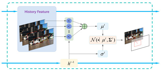
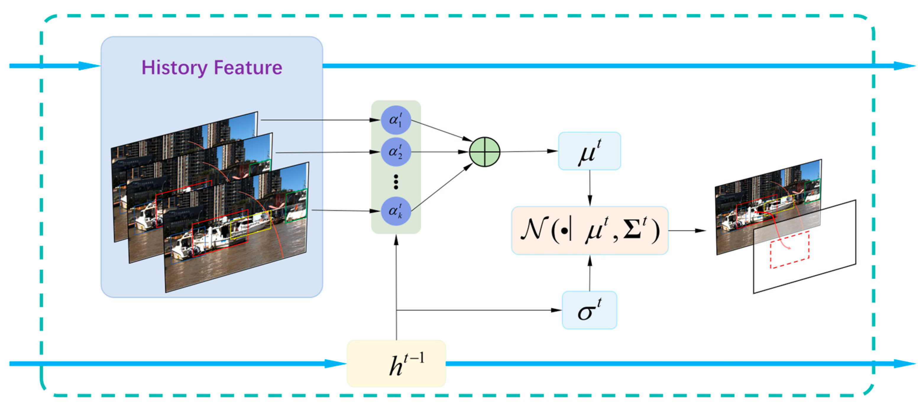
After detection, the system must solve cross-frame data association. We introduce a RAN to model target appearance and motion temporally, as shown in Figure 3. Using hidden states containing historical information, the system matches new detections with existing trajectories.
Figure 3.
RAN Framework.
The model receives input vectors from time step 1 to k. It estimates the conditional probability distribution of the current input . This process can be expressed as the weighted sum of historical inputs plus Gaussian noise:
where is Gaussian noise. To determine the importance of different historical moments, weights are dynamically generated via an attention mechanism:
We construct an attention layer using the current query and historical keys . Assuming the noise term follows a normal distribution with zero mean and standard deviation:
Therefore, the predicted mean and variance are:
In the RAN model, weights and standard deviation change over time. This allows the model to adjust its estimation strategy as input features change.
To capture long-term trends and estimate and , a gated recurrent unit (GRU) is embedded. It maintains a hidden state as an internal parameter. At each step , the GRU updates based on input and the previous state . Based on the current hidden state, the parameters of the autoregressive model are estimated via a mapping function :
where is a fully connected layer containing specific element-wise transformations:
The Softmax function ensures weights sum to 1, while Softplus ensures the standard deviation is greater than 0. This guarantees accurate estimation of the conditional probability distribution .
Given a set of detections, the system must determine the relationship between each new object and existing trajectories. Let be the trajectory index and be the current detection. We extract appearance features and dynamic motion features from the bounding box. For trajectory , let the historical boxes and appearance features be and . The association score between trajectory and object is defined as the joint conditional probability:
Both appearance and bounding box features are modeled using RAN, assuming they are independent. If the score exceeds a threshold, object is associated with the highest-scoring trajectory . Otherwise, object is not associated and is marked as lost.
Since appearance and motion differ significantly, we use two sets of hidden states and external parameters . During tracking, when a new detection is associated, both memory types update. The probabilities and are derived independently and then combined. When association fails, only the motion prediction updates, while appearance parameters remain unchanged.
3.3. BEV Mapping and Fusion Velocity Update
3.3.1. Compensation-Based BEV Mapping
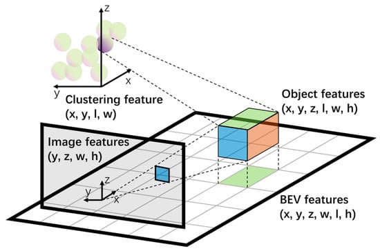
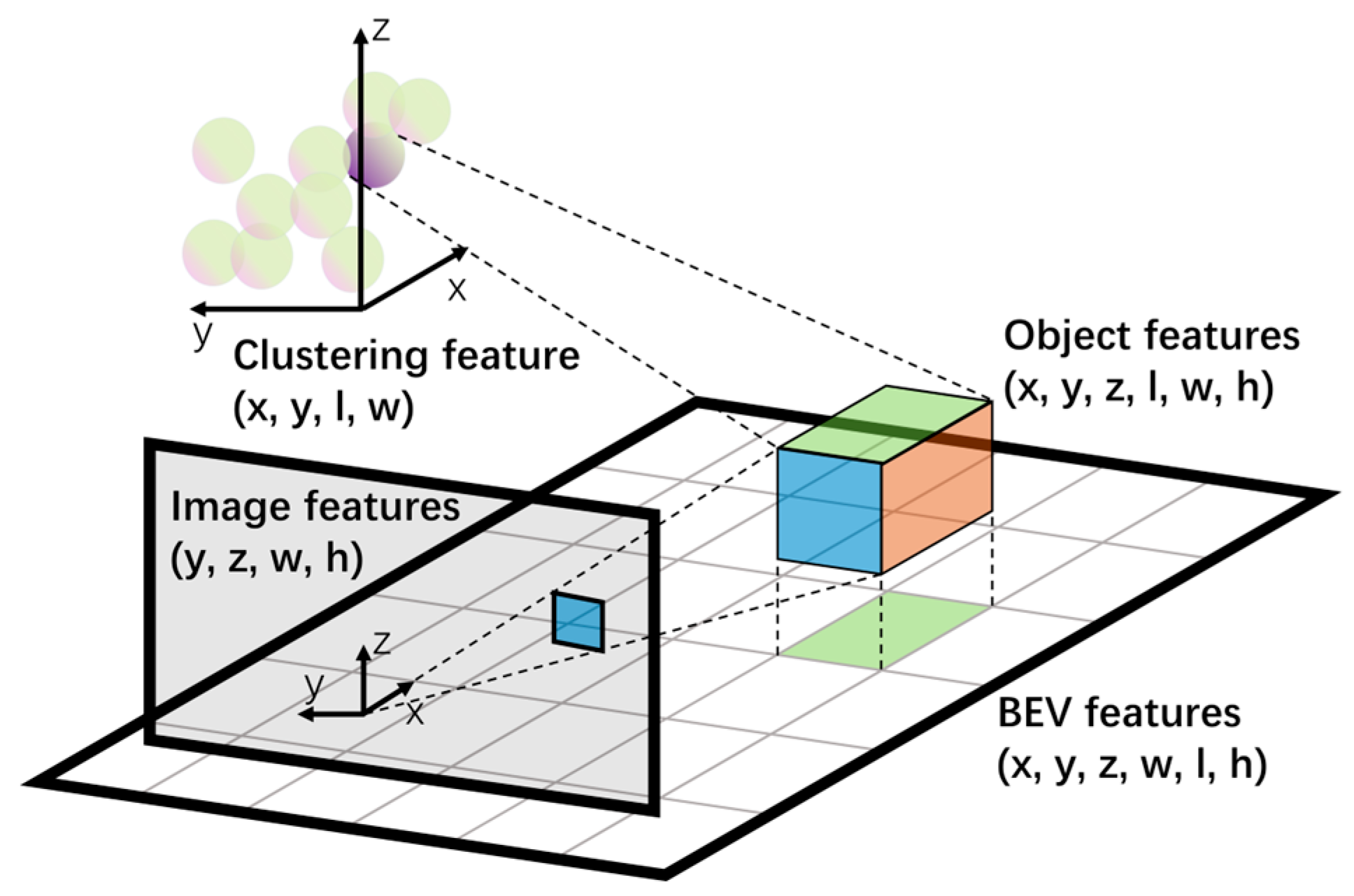
After obtaining the corrected depth distribution and semantic features , the core task is to transform perspective features into a vessel-centric BEV, as shown in Figure 4. This facilitates subsequent motion planning. However, USVs face 6-DOF motion challenges on water. Specifically, roll and pitch cause severe geometric distortion in projection methods that assume flat ground. To address this, we designed an LSS pipeline that includes attitude compensation.
Figure 4.
Schematic diagram of BEV transformation.
First, pixels are lifted into frustum coordinates by calculating the outer product of semantic features and depth distribution. Subsequently, to eliminate the effects of hull vibration, the system introduces real-time attitude correction during back-projection. Using real-time inertial measurement unit (IMU) attitude data, we construct a rotation matrix . Combining this with camera intrinsics and extrinsics , the frustum features are mapped to the BEV plane:
where and represent roll, pitch, and yaw angles, respectively. This explicitly cancels camera optical axis shifts caused by waves, ensuring the spatial stability of the BEV feature map.
3.3.2. Radar-Guided EKF State Update
In water scenes, velocity estimation relies directly on positional accuracy in the BEV space. However, due to scale drift in monocular depth and BEV projection, velocity estimation suffers from jitter and lag. In contrast, radar provides instantaneous radial Doppler velocity but lacks tangential information. Therefore, an EKF with a flexible observation model is proposed. The state vector of the i-th target at time k is defined as . Here, denote the position in the BEV plane, resultant velocity, and heading angle, respectively. Assuming the target follows a constant velocity model over a short period, the equation is:
where is the state transition matrix, and and represent process noise. To handle missed detections in vision or radar, the observation model and function are dynamically switched based on the radar association status.
When a target is captured only by vision, the observation vector contains only position information . In this case, is linear, and the filter degenerates into a standard Kalman Filter. It uses historical trajectories to smooth visual position jitter. If radar successfully captures the target, the observation vector extends to . Since radial velocity is a non-linear function of resultant velocity and relative angle in the state vector:
At this point, the Jacobian matrix is calculated to complete the EKF update. Using radar physical measurements to directly constrain the state space eliminates cumulative errors from visual differentiation. This allows velocity estimation to converge rapidly within a few frames. Combined with target association from the RAN module, the system achieves robust state tracking of dynamic water targets.
4. Experiments and Analysis
4.1. Experimental Settings
4.1.1. Datasets
The training phase primarily utilizes the WaterScenes [45] dataset. Unlike other marine datasets that provide only image data, WaterScenes synchronously collects and annotates visual and radar information. This supports systematic research on radar–vision fusion algorithms.
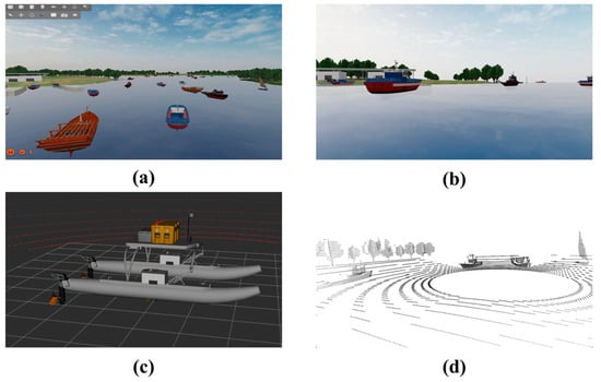
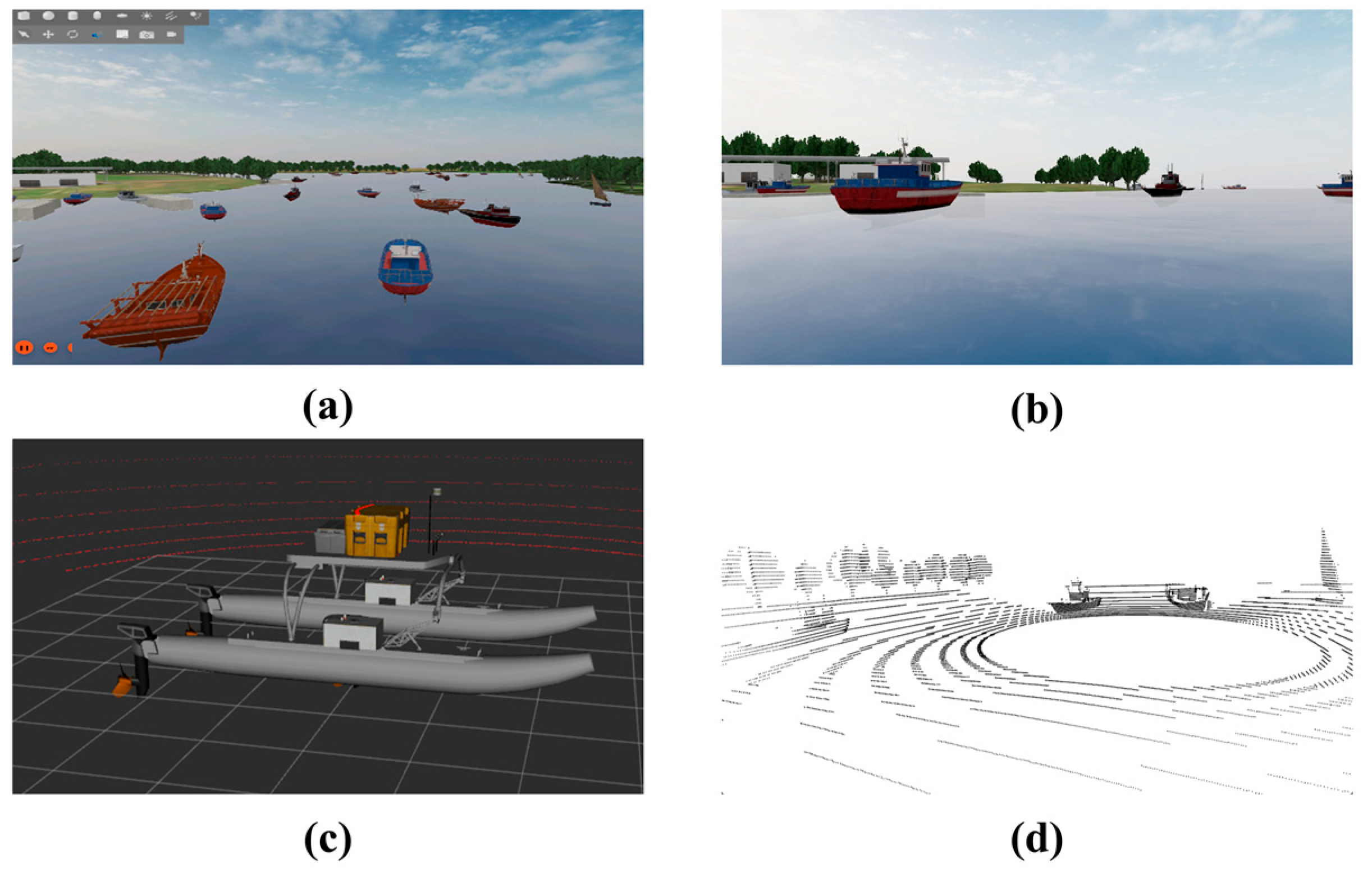
Furthermore, to improve algorithm robustness in complex water environments and address data scarcity in extreme conditions, a dynamic water surface simulation environment was built using Gazebo within the ROS framework (Figure 5). A simulated dataset was collected and annotated in this environment. It contains 62 object instances covering 11 typical water surface classes, including sailboats, yachts, and buoys.
Figure 5.
Simulation Environment: (a) Simulated water-surface environment; (b) RGB image; (c) USV model; (d) radar point cloud.
The platform supports dynamic adjustments of environmental factors like light intensity and wave height. This reproduces various maritime navigation scenes. Combining simulated and real data ensures diversity and improves model generalization in complex environments.
The WaterScenes dataset serves as the primary source for model training and the quantitative evaluation of perception performance (including object detection, semantic segmentation, and depth estimation). The Gazebo-based simulated dataset is utilized to supplement complex multi-target port scenarios, thereby enhancing the model’s robustness during the training process. Finally, data collected from the real USVs platform is exclusively applied for qualitative visual verification and real-time deployment assessment in real-world environments.
Specifically, the dataset used in our experiments contains a total of 58,540 synchronized image and radar frames. The original image resolution is 1920 × 1080 pixels. The entire dataset was divided into training and validation sets at a ratio of 8:2, resulting in 46,832 samples for model training and 11,708 samples for the validation set. All quantitative evaluations (Table 1, Table 2 and Table 3) were conducted on this validation set, which effectively serves as our test set. Regarding the radar data, the employed millimeter-wave radar provides multi-dimensional point clouds. For each reflected target, the radar point contains essential physical measurements, including 3D spatial coordinates, radial Doppler velocity, and Radar Cross Section. These features are crucial for our subsequent depth correction and velocity state updates.
Table 1.
Comparison of perception algorithm performance. (Evaluated on the WaterScenes dataset).
Table 2.
Ablation study of radar constraints. (Evaluated on the WaterScenes dataset).
Table 3.
RAN ablation experiment. (Evaluated on the WaterScenes dataset).
4.1.2. Baseline Models
To evaluate the proposed improvements, two baseline systems were constructed for comparison. Both baselines and Geo-RVF share the same visual backbone, detection framework, and training data. They differ only in multi-modal fusion strategies and motion modeling methods.
The Vision Baseline operates as a pure vision USV perception system, utilizing only visual inputs without any radar information. It implements object detection and segmentation based on YOLO-AFM and constructs BEV representations via a monocular depth estimation model, where target velocity is estimated by differentiating adjacent BEV positions.
The Vision + EKF Baseline augments the purely visual framework with an EKF to explicitly model motion states. Although this system still relies exclusively on visual observations, it is designed to verify the improvements in motion estimation stability provided by traditional filtering techniques when direct physical velocity constraints are absent.
The relevance of establishing these two specific baseline models is to serve as systematic ablation benchmarks. By comparing Geo-RVF against the ‘Vision Baseline’, we can quantitatively demonstrate the necessity of radar geometric priors in resolving visual depth scale drift. Furthermore, comparing Geo-RVF against the ‘Vision + EKF Baseline’ isolates and validates the contribution of our proposed RAN module and radar Doppler velocity in achieving stable temporal tracking compared to traditional purely kinematic filtering.
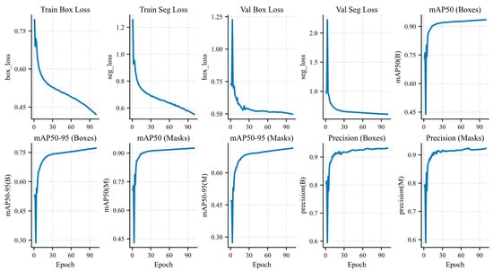
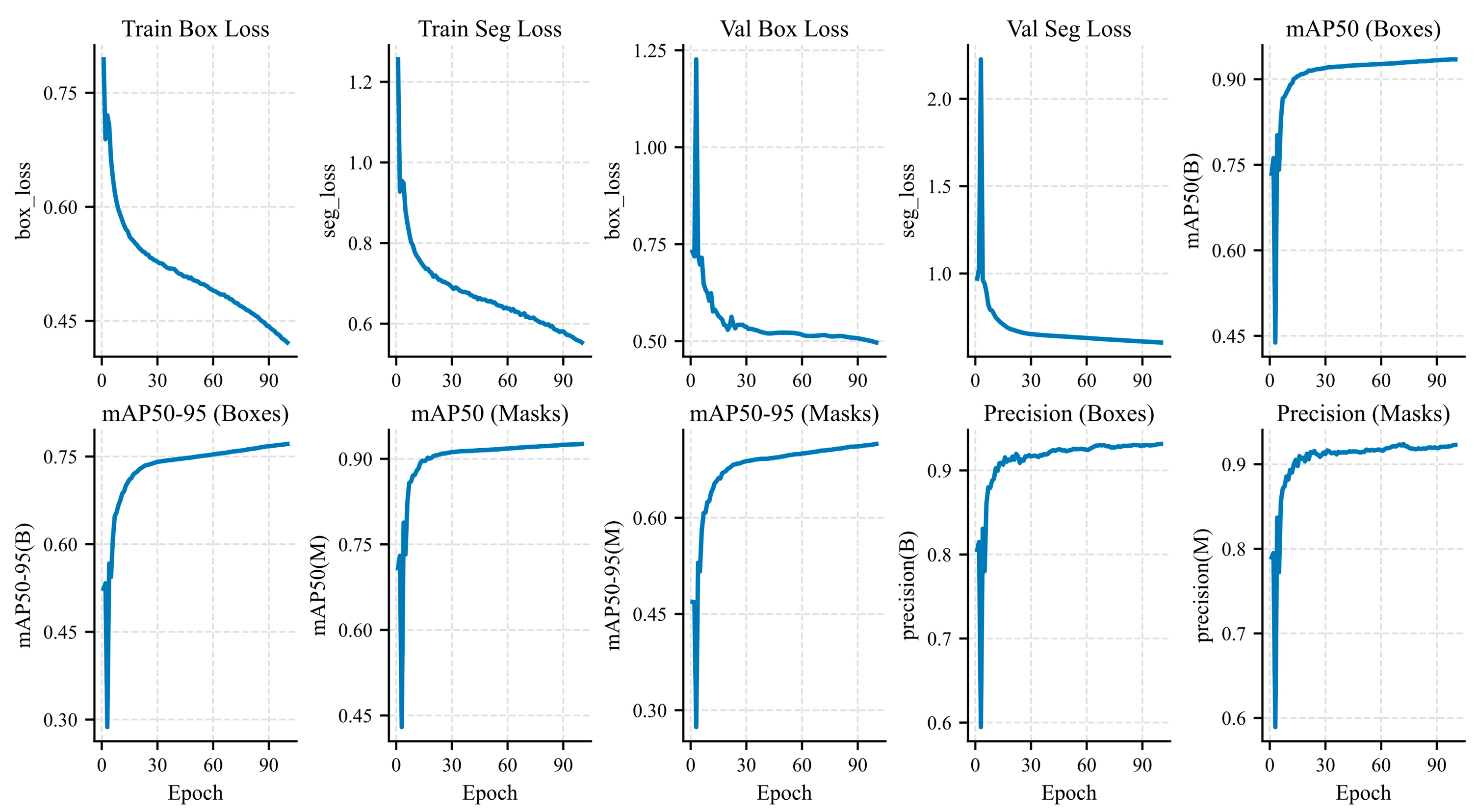
The proposed method further introduces radar data to achieve cross-modal depth scale correction and radar-aware motion estimation. Figure 6 illustrates key training metrics, including loss, detection accuracy, and segmentation accuracy. These metrics indicate effective model convergence. After applying pruning techniques, high detection accuracy is maintained, achieving 82.5% in mean average precision (mAP) 50–90.
Figure 6.
Loss and accuracy changes during visual model training. (Evaluated on the WaterScenes and simulated datasets).
4.1.3. Experimental Details
All models were implemented using PyTorch2.2.1 and CUDA12.7. Experiments used the AdamW optimizer with an initial learning rate of 1 × 10⁻⁴. Weight decay was set to 0.5. Cosine annealing was used as the learning rate scheduler, decaying to 0.1 starting from 40% of the training process. During both training and inference, to balance perception accuracy and the limited computational resources of edge devices, the input images for all models were uniformly resized to 640 × 640 pixels. The number of epochs was set to 100 with a batch size of 16. Training took 33 h on an RTX 3090 (NVIDIA, Santa Clara, CA, USA). Data was uniformly split into training and validation sets. All comparison methods were trained using the same dataset and strategy. During inference, all methods used identical input resolutions and post-processing pipelines. The system was deployed and tested on a Jetson Orin NX (NVIDIA, Santa Clara, CA, USA) to evaluate real-time performance.
4.2. Perception Performance Evaluation and Analysis
To verify the effectiveness of the method in water surface perception, state-of-the-art and classic models suitable for aquatic environments were selected for comparison. Performance was evaluated based on object detection, semantic segmentation, and detection efficiency. As shown in Table 1, Geo-RVF achieved optimal performance in object detection.
Regarding detection performance, traditional two-stage methods (e.g., Faster R-CNN [46], Mask R-CNN [47]) offer high accuracy but require significant computational resources, making them unsuitable for real-time edge deployment. Lightweight one-stage methods (e.g., YOLOv5-T, YOLOv8-N) offer fast inference but suffer from reduced accuracy in complex water scenes due to lighting changes and scale uncertainty. Joint detection and segmentation models (YOLOP [48], HybridNets [49]) perform stably in segmentation but are limited by errors inherent to pure visual input.
In contrast, both Achelous [50] and the proposed method incorporate radar data, significantly outperforming pure vision solutions. This validates the effectiveness of radar geometric priors in water environments. The proposed method achieved the best results in mAP50, mAP50–90, and AR50–90 metrics, while maintaining leading performance in segmentation accuracy. While a pure 2D vision model like YOLOv8-N achieves a higher FPS, it inherently lacks depth estimation, radar fusion, and 3D BEV transformation capabilities. In the specific domain of 3D multi-modal BEV perception, mainstream frameworks (e.g., BEVFormer or TransFusion) typically require massive computational resources (often exceeding 100 GFLOPs), making them unviable for USV edge devices. Although our Geo-RVF has slightly higher FLOPs than the highly optimized Achelous, this marginal increase in computation is deliberately traded for superior perception accuracy and enhanced robustness in depth correction. By compressing a complete multi-modal 3D BEV pipeline into just 10.3 GFLOPs and maintaining an inference speed of over 50 FPS (23 FPS on an edge device), Geo-RVF demonstrably achieves a lightweight status while providing a stable and reliable foundation for subsequent depth correction and BEV construction.
4.2.1. Depth Estimation and BEV Quality Analysis
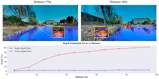
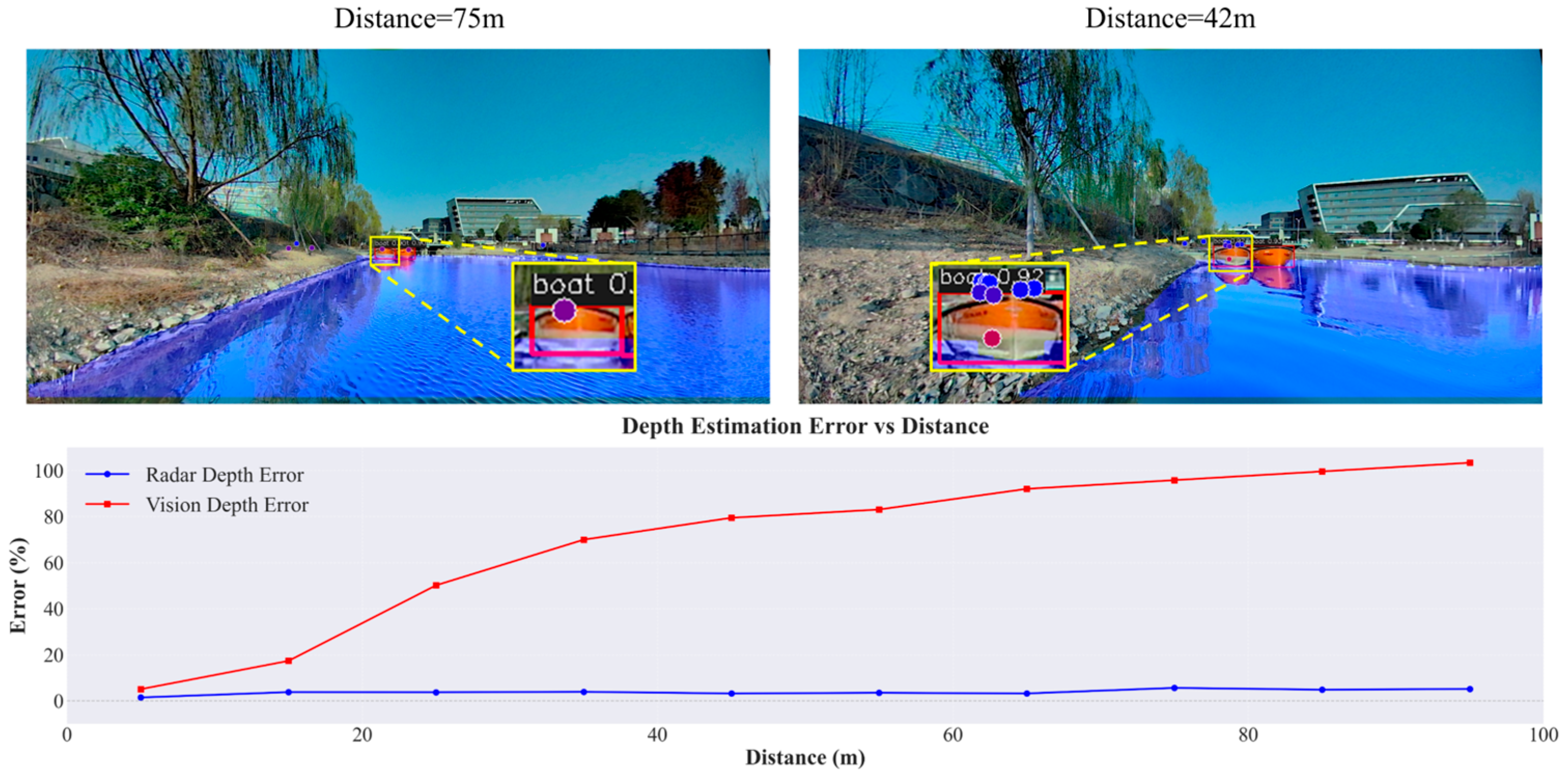
Accurate depth is the foundation of BEV construction. Depth estimation errors were analyzed across different distance intervals. As shown in Figure 7, the number of radar points detected on targets decreases with distance. Beyond 80 m, fewer than five points match the bounding box. Pure vision methods exhibit significant scale drift for distant targets. Introducing radar constraints significantly improved depth accuracy in target regions, maintaining stable spatial positioning across all distances. While hard radar constraints limit error growth, they risk propagation errors when point cloud matching fails. In contrast, the proposed depth correction based on probability consistency maintained a low and stable error level across the full range.
Figure 7.
Visualization of point cloud projection. (Qualitative results from the real USVs platform).
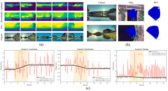
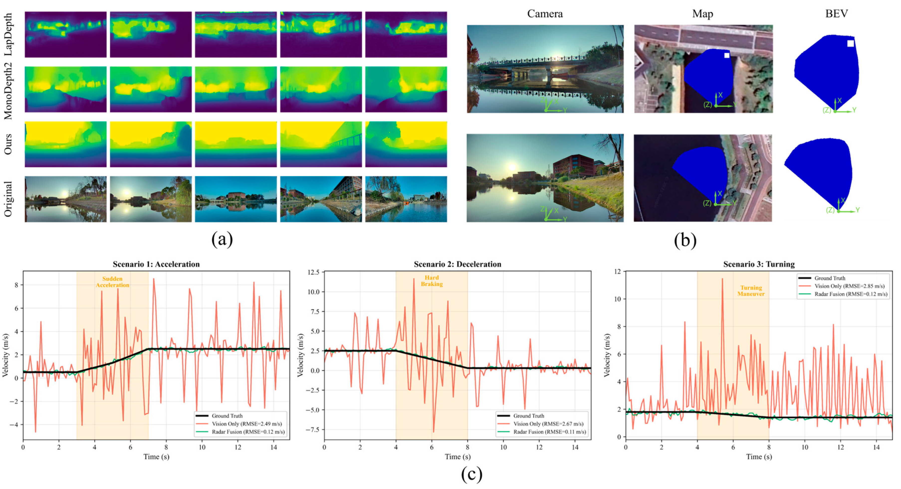
In Figure 9a, baseline methods correct depth near contact points, but this constraint acts only locally. This often causes depth mutations at target boundaries, disrupting the continuity of the depth field. Geo-RVF uses radar measurements as soft constraints and diffuses them along the water surface. Consequently, the method maintains low depth errors even in distant water regions.
To evaluate the spatial structural validity of the BEV representation, the generated BEV water area was compared with a real map (Figure 9b). The shoreline trend in the generated BEV aligns with the satellite map, showing no obvious deformation or structural breaks.
4.2.2. Robustness in Complex Lighting Scenarios
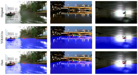
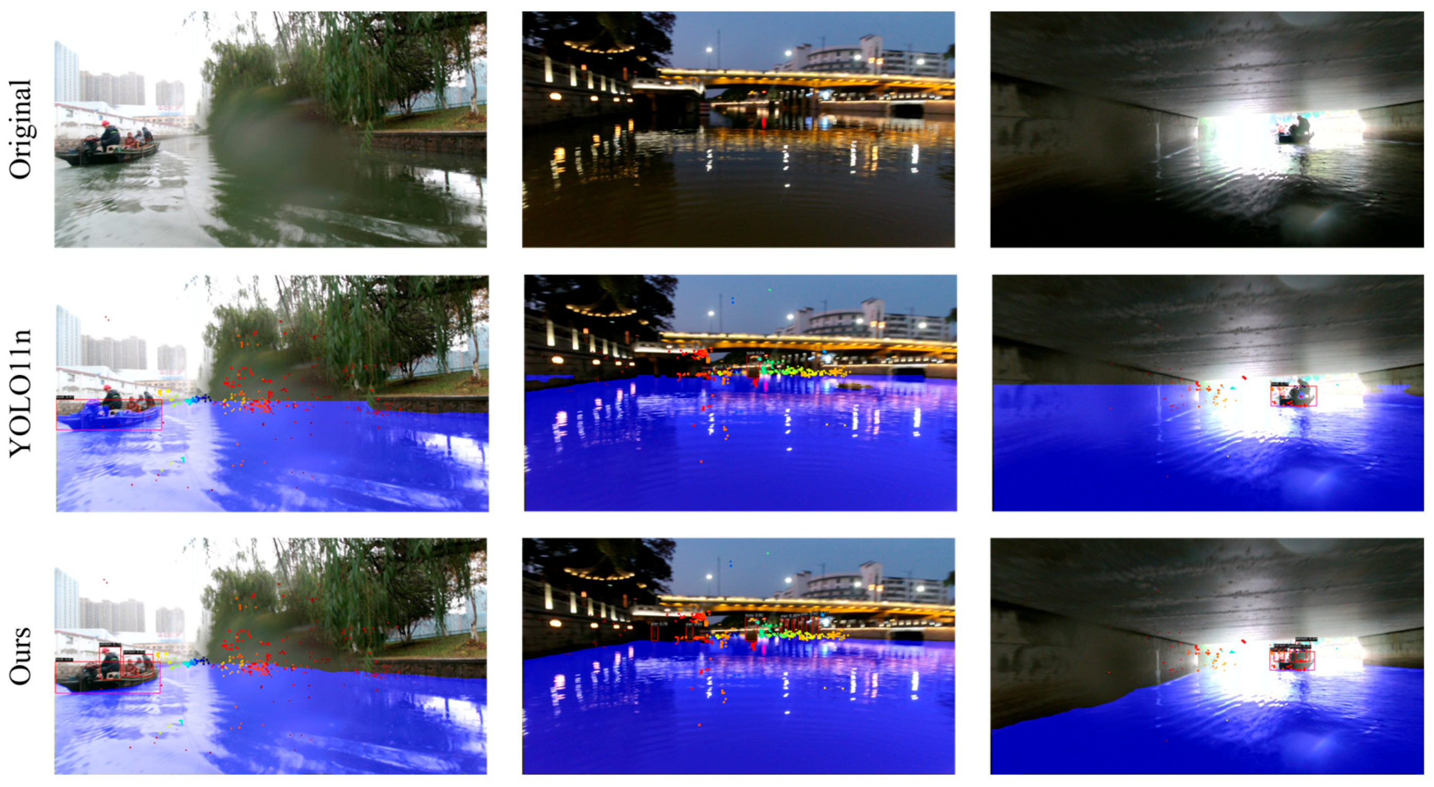
To verify the stability of this system under complex lighting conditions, this study conducted a qualitative comparison between the pure visual benchmark and Geo-RVF. As shown in Figure 8, pure visual perception relies entirely on texture and gradient features, but when pixels are overexposed due to sunlight glare or underexposed at night due to insufficient light, these features are easily damaged or completely disappear. Therefore, models relying solely on vision will suffer from severe missed detections.
Figure 8.
Complex Lighting Comparison Chart.
In contrast, by introducing radar spatial anchors and using an adaptive feature module to fuse multimodal features, our radar visual fusion system effectively utilizes radar echoes to penetrate visual interference. Even when interfered with by strong light when crossing an archway, the radar can provide highly reliable spatial cues. As shown in Figure 8, our fusion system successfully restored the bounding boxes under these unfavorable conditions and maintained accurate navigation area segmentation, demonstrating adaptability to diffuse lighting environments.
4.3. Dynamic Tracking Performance and Ablation Study
4.3.1. Velocity Estimation Accuracy in Motion Scenarios
Three typical motion scenarios were set up for a target boat navigating open waters. The velocity estimation differences between the pure vision scheme and the fusion scheme were compared using root mean square error (RMSE) (Figure 9c). Baseline methods showed high variance. Specifically, baselines rely on differentiating target positions between adjacent frames, which causes lag during acceleration or deceleration. By fusing radar Doppler velocity, the system reflected real-time speed changes with an RMSE of only 0.12 m/s. In turning scenarios, baseline methods occasionally lost targets, whereas the radar method significantly improved stability by directly constraining the motion state via radial velocity.
Figure 9.
(a) Visualization comparison of depth estimation; (b) BEV visualization comparison. To intuitively evaluate spatial correctness, the generated BEV drivable areas (blue masks) are overlaid onto corresponding global maps. An ego-vessel coordinate system is also overlaid to illustrate the viewpoint transformation. (c) Velocity estimation comparison in three scenarios. (Qualitative results from the real USVs platform).
Results indicate that after introducing radar information, the system can directly correct motion states using Doppler velocity. RMSE decreased from approximately 2.5–2.8 m/s to 0.1–0.2 m/s, enhancing perception stability in dynamic real-world environments.
4.3.2. Ablation Experiments
Table 2 shows that BEV mapping accuracy benefits from point cloud priors, outperforming pure radar-guided depth estimation. However, using 3D point cloud hard constraints proved ineffective and unreasonable. To address this, a depth correction method based on probability consistency modeling was proposed. By fusing radar ranging and visual features at the probability distribution level, depth estimation for objects improved significantly. Furthermore, combining this with a contact point diffusion strategy allowed depth constraints to propagate smoothly across the water surface, ensuring geometric consistency while avoiding local depth mutations.
To evaluate the dynamic tracking performance of the RAN module in Table 3, we constructed a multi-object tracking evaluation set. This subset consists of five consecutive video sequences selected from the validation set, totaling 64 unique dynamic targets. The selected scenarios include target intersections, partial occlusions, and severe scale changes during relative motion. This is to test the robustness of the algorithm in terms of identity switching and trajectory fragmentation. To verify the effectiveness of the RAN, an ablation analysis was performed on the association module, as shown in Table 3. Introducing Appearance-RAN reduced trajectory interruptions by eight times, increased the max tracking length to 82 frames, and improved Multi-Object Tracking Accuracy (MOTA) by 6.2%. This confirms the module effectively models geometric contours and scale changes in the BEV space, improving robustness under short-term occlusion. Introducing only the Motion-RAN module improved stability under complex motion conditions. Trajectory interruptions dropped to 16, max tracking length rose to 89 frames, and MOTA increased to 78.1%. This module achieved temporal modeling of acceleration and turning, aligning state prediction with physical motion constraints.
When both Appearance-RAN and Motion-RAN were introduced without the autoregressive fusion strategy, performance improved but remained limited in trajectory continuity. In contrast, the proposed joint autoregressive association model synergistically modeled appearance and motion. This reduced trajectory interruptions to seven, extended stable tracking to 112 frames, and raised MOTA to 84.6%. This demonstrates that the autoregressive fusion mechanism effectively accumulates historical association information and suppresses uncertainty propagation.
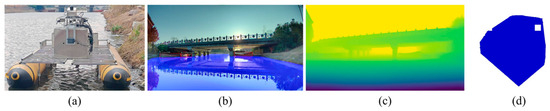
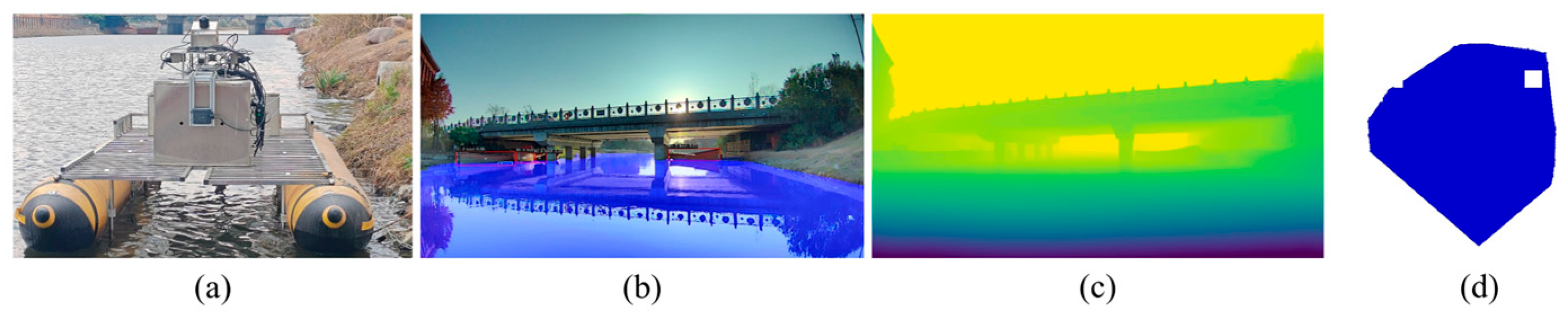
4.4. Real-Ship Deployment and Performance Verification
Figure 10a shows the USVs platform used for water surface perception. The platform measures 2 × 5 m with a maximum speed of 2 m/s. It integrates multi-source sensors, including an RGB camera (SG2-IMX390C-5200-G2A, Sensing World, Shenzhen, China; FOV = 118° × 62°), Airy LiDAR (RoboSense, Shenzhen, China), and a positioning module (FSS-NAV680-SA, FORSENSE, Shanghai, China; IMU, real-time kinematic (RTK) and Global Positioning System (GPS)). All perception and fusion algorithms run on an Nvidia Orin NX edge computing platform (8 GB RAM, 70 TOPS). A sensor fusion strategy combines data from the camera, LiDAR, GPS, and IMU to enhance object detection. This framework facilitates the transition of algorithms to real-world USVs platforms.
Figure 10.
Algorithm Operation Diagram. (a) USV platform and perception sensors; (b) detection and segmentation; (c) depth estimation; (d) BEV. The controllable viewing area in (b) is geometrically transformed into the top-down view space in (d). In this figure, the ships detected on the right side of (b) are accurately mapped to the white void area (which is non-navigable) in the upper-right corner of the bounding box map (d). (Qualitative results from the real USVs platform).
On the software level, the system includes sensor drivers, time synchronization mechanisms, and coordinate transformation modules. Without optimization, the system occupied 2.6 GB memory, 30% CPU, and 75% GPU, with an output frequency of 12 FPS. After TensorRT acceleration optimization, GPU utilization increased by 8%, and the frame rate rose to 22 FPS, ensuring responsiveness under dynamic conditions.
5. Conclusions
To address core challenges in USV navigation, such as visual depth drift, motion estimation lag, and limited edge computing resources, a lightweight radar–vision fusion perception system named Geo-RVF is proposed. The system enhances perception robustness through dual geometric and temporal physical constraints. To resolve scale uncertainty in open waters, a probabilistic depth correction mechanism based on radar geometric anchors is designed. By utilizing the target-water contact region, sparse radar ranging is converted into soft constraints. This effectively suppresses water clutter interference and corrects scale deviations in BEV mapping. Furthermore, a tracking framework combining RAN and EKF is constructed. The long-term memory of RAN resolves association difficulties caused by texture degradation. Additionally, radar Doppler velocity is introduced to correct visual observation lag in real time, significantly reducing velocity estimation errors. Experiments demonstrate that the TensorRT-optimized Geo-RVF achieves real-time inference of 23 FPS on the Jetson Orin NX. Its detection accuracy of 44.2% mAP and segmentation performance of 99% mean intersection over union (mIoU) outperform existing mainstream lightweight models. Future work will focus on integrating infrared thermal sensors to address night perception limitations and exploring geometric self-supervised learning paradigms to further improve generalization and autonomous decision making in extreme sea conditions.
Author Contributions
Literature search, J.Z.; Research design, J.Z. and Z.T.; Data collection, Y.L.; Software, J.Z. and Z.H.; Resources, Y.L.; Data organization, Y.Y.; Manuscript writing, J.Z. and Z.H.; Review and editing, G.Z.; Visualization, Z.H.; Supervision, Z.T. All authors have read and agreed to the published version of the manuscript.
Funding
This research was supported by the Hainan Province’s Key Research and Development Project (Grant No. ZDYF2023GXJS023) and the Marine Industry Science and Technology Project of Zhejiang Province (Grant No. 2026HYB02007).
Data Availability Statement
Dataset available on request from the authors.
Acknowledgments
The authors would like to thank the funder for supporting them and the editor and reviewers for their constructive comments.
Conflicts of Interest
The authors declare no conflicts of interest.
Abbreviations
The following abbreviations are used in this manuscript:
| USVs | Unmanned Surface Vehicles |
| RAN | Recurrent Autoregressive Network |
| BEV | Bird’s-Eye View |
| EKF | Extended Kalman Filter |
| ROI | Region of Interest |
| FCN | Fully Convolutional Networks |
| GAN | Generative Adversarial Networks |
| GNN | Graph Neural Networks |
| AFM | Adaptive Feature Module |
| GRU | Gated Recurrent Unit |
| RMSE | Root Mean Square Error |
| mAP | mean Average Precision |
| mIoU | mean Intersection over Union |
| IMU | Inertial Measurement Unit |
| RTK | Real-Time Kinematic |
| GPS | Global Positioning System |
References
- Barrera, C.; Padron Armas, I.; Luis, F.; Llinas, O.; Marichal, N. Trends and Challenges in Unmanned Surface Vehicles (USV): From Survey to Shipping. TransNav Int. J. Mar. Navig. Saf. Sea Transp. 2021, 15, 135–142. [Google Scholar] [CrossRef] [Scilit]
- Yao, S.; Guan, R.; Huang, X.; Li, Z.; Sha, X.; Yue, Y.; Lim, E.G.; Seo, H.; Man, K.L.; Zhu, X.; et al. Radar-Camera Fusion for Object Detection and Semantic Segmentation in Autonomous Driving: A Comprehensive Review. IEEE Trans. Intell. Veh. 2024, 9, 2094–2128. [Google Scholar] [CrossRef] [Scilit]
- Srivastav, A.; Mandal, S. Radars for Autonomous Driving: A Review of Deep Learning Methods and Challenges. IEEE Access 2023, 11, 97147–97168. [Google Scholar] [CrossRef] [Scilit]
- Nabati, R.; Qi, H. CenterFusion: Center-Based Radar and Camera Fusion for 3D Object Detection. In Proceedings of the 2021 IEEE Winter Conference on Applications of Computer Vision (WACV), Waikoloa, HI, USA, 3–8 June 2021; IEEE: New York, NY, USA, 2021; pp. 1526–1535. [Google Scholar]
- Bai, X.; Hu, Z.; Zhu, X.; Huang, Q.; Chen, Y.; Fu, H.; Tai, C.-L. TransFusion: Robust LiDAR-Camera Fusion for 3D Object Detection with Transformers. In Proceedings of the 2022 IEEE/CVF Conference on Computer Vision and Pattern Recognition (CVPR), New Orleans, LA, USA, 18–24 June 2022; IEEE: New York, NY, USA, 2022; pp. 1080–1089. [Google Scholar]
- Liu, Z.; Tang, H.; Amini, A.; Yang, X.; Mao, H.; Rus, D.L.; Han, S. BEVFusion: Multi-Task Multi-Sensor Fusion with Unified Bird’s-Eye View Representation. In Proceedings of the 2023 IEEE International Conference on Robotics and Automation (ICRA), London, UK, 29 May–2 June 2023; IEEE: New York, NY, USA, 2023; pp. 2774–2781. [Google Scholar]
- Philion, J.; Fidler, S. Lift, Splat, Shoot: Encoding Images from Arbitrary Camera Rigs by Implicitly Unprojecting to 3D. In Computer Vision—ECCV 2020; Vedaldi, A., Bischof, H., Brox, T., Frahm, J.-M., Eds.; Lecture Notes in Computer Science, Vol. 12359; Springer International Publishing: Cham, Switzerland, 2020; pp. 194–210. [Google Scholar]
- Zhou, J.; Zhang, G.; Liu, Y.; Sun, W.; Luo, Z.; Li, Z. Lightweight Multi-Task Perception for USV Navigation with Adaptive Feature Fusion. IFAC-PapersOnLine 2025, 59, 633–638. [Google Scholar] [CrossRef] [Scilit]
- Yadav, R.; Vierling, A.; Berns, K. Radar + RGB Fusion for Robust Object Detection in Autonomous Vehicle. In Proceedings of the 2020 IEEE International Conference on Image Processing (ICIP), Abu Dhabi, United Arab Emirates, 25–28 October 2020; IEEE: New York, NY, USA, 2020; pp. 1986–1990. [Google Scholar]
- Kurniawan, I.T.; Trilaksono, B.R. ClusterFusion: Leveraging Radar Spatial Features for Radar-Camera 3D Object Detection in Autonomous Vehicles. IEEE Access 2023, 11, 121511–121528. [Google Scholar] [CrossRef] [Scilit]
- Kim, Y.; Kim, S.; Choi, J.W.; Kum, D. CRAFT: Camera-Radar 3D Object Detection with Spatio-Contextual Fusion Transformer. Proc. AAAI Conf. Artif. Intell. 2023, 37, 1160–1168. [Google Scholar] [CrossRef] [Scilit]
- Li, Z.; Yuan, T.; Ma, L.; Zhou, Y.; Peng, Y. Target Detection for USVs by Radar–Vision Fusion with Swag-Robust Distance-Aware Probabilistic Multimodal Data Association. IEEE Sens. J. 2024, 24, 20177–20187. [Google Scholar] [CrossRef] [Scilit]
- He, X.; Wu, D.; Wu, D.; You, Z.; Zhong, S.; Liu, Q. Millimeter-Wave Radar and Camera Fusion for Multiscenario Object Detection on USVs. IEEE Sens. J. 2024, 24, 31562–31572. [Google Scholar] [CrossRef] [Scilit]
- Hwang, J.-J.; Kretzschmar, H.; Manela, J.; Rafferty, S.; Armstrong-Crews, N.; Chen, T.; Anguelov, D. CramNet: Camera-Radar Fusion with Ray-Constrained Cross-Attention for Robust 3D Object Detection. In Proceedings of the Computer Vision—ECCV 2022; Avidan, S., Brostow, G., Cissé, M., Farinella, G.M., Hassner, T., Eds.; Springer Nature: Cham, Switzerland, 2022; pp. 388–405. [Google Scholar]
- Kim, J.; Seong, M.; Bang, G.; Kum, D.; Choi, J.W. RCM-Fusion: Radar-Camera Multi-Level Fusion for 3D Object Detection. In Proceedings of the 2024 IEEE International Conference on Robotics and Automation (ICRA), Yokohama, Japan, 13–17 May 2024; IEEE: New York, NY, USA, 2024; pp. 18236–18242. [Google Scholar]
- Li, Z.; Wang, W.; Li, H.; Xie, E.; Sima, C.; Lu, T.; Yu, Q.; Dai, J. BEVFormer: Learning Bird’s-Eye-View Representation from LiDAR-Camera via Spatiotemporal Transformers. IEEE Trans. Pattern Anal. Mach. Intell. 2025, 47, 2020–2036. [Google Scholar] [CrossRef] [Scilit] [PubMed]
- Xu, W.; Meng, X.; Hu, Y.; Deng, H. RCFusionNet: A Radar-Guided Two-Stage Fusion Approach to Effective Multimodal Perception. IEEE Sens. J. 2025, 25, 33890–33900. [Google Scholar] [CrossRef] [Scilit]
- Xu, D.; Wang, W.; Tang, H.; Liu, H.; Sebe, N.; Ricci, E. Structured Attention Guided Convolutional Neural Fields for Monocular Depth Estimation. In Proceedings of the 2018 IEEE/CVF Conference on Computer Vision and Pattern Recognition, Salt Lake City, UT, USA, 18–23 June 2018; IEEE: New York, NY, USA, 2018; pp. 3917–3925. [Google Scholar]
- Rajapaksha, U.; Sohel, F.; Laga, H.; Diepeveen, D.; Bennamoun, M. Deep Learning-Based Depth Estimation Methods from Monocular Image and Videos: A Comprehensive Survey. ACM Comput. Surv. 2024, 56, 315. [Google Scholar] [CrossRef] [Scilit]
- Farooq Bhat, S.; Alhashim, I.; Wonka, P. AdaBins: Depth Estimation Using Adaptive Bins. In Proceedings of the 2021 IEEE/CVF Conference on Computer Vision and Pattern Recognition (CVPR), Nashville, TN, USA, 20–25 June 2021; IEEE: New York, NY, USA, 2021; pp. 4008–4017. [Google Scholar]
- Eigen, D.; Puhrsch, C.; Fergus, R. Depth Map Prediction from a Single Image Using a Multi-Scale Deep Network. In Proceedings of the Advances in Neural Information Processing Systems; Curran Associates, Inc.: Red Hook, NY, USA, 2014; Volume 27. [Google Scholar]
- Laina, I.; Rupprecht, C.; Belagiannis, V.; Tombari, F.; Navab, N. Deeper Depth Prediction with Fully Convolutional Residual Networks. In Proceedings of the 2016 Fourth International Conference on 3D Vision (3DV), Stanford, CA, USA, 25–28 October 2016; pp. 239–248. [Google Scholar]
- Silberman, N.; Hoiem, D.; Kohli, P.; Fergus, R. Indoor Segmentation and Support Inference from RGBD Images. In Proceedings of the Computer Vision—ECCV 2012; Fitzgibbon, A., Lazebnik, S., Perona, P., Sato, Y., Schmid, C., Eds.; Springer: Berlin/Heidelberg, Germany, 2012; pp. 746–760. [Google Scholar]
- Ummenhofer, B.; Zhou, H.; Uhrig, J.; Mayer, N.; Ilg, E.; Dosovitskiy, A.; Brox, T. DeMoN: Depth and Motion Network for Learning Monocular Stereo. In Proceedings of the 2017 IEEE Conference on Computer Vision and Pattern Recognition (CVPR), Honolulu, HI, USA, 21–26 July 2017; IEEE: New York, NY, USA, 2017; pp. 5622–5631. [Google Scholar]
- Zhou, T.; Brown, M.; Snavely, N.; Lowe, D.G. Unsupervised Learning of Depth and Ego-Motion from Video. In Proceedings of the 2017 IEEE Conference on Computer Vision and Pattern Recognition (CVPR), Honolulu, HI, USA, 21–26 July 2017; IEEE: New York, NY, USA, 2017; pp. 6612–6619. [Google Scholar]
- Garg, R.; VijayKumar, B.G.; Carneiro, G.; Reid, I. Unsupervised CNN for Single View Depth Estimation: Geometry to the Rescue. In Proceedings of the Computer Vision—ECCV 2016; Leibe, B., Matas, J., Sebe, N., Welling, M., Eds.; Springer International Publishing: Cham, Switzerland, 2016; pp. 740–756. [Google Scholar]
- Godard, C.; Aodha, O.M.; Brostow, G.J. Unsupervised Monocular Depth Estimation with Left-Right Consistency. In Proceedings of the 2017 IEEE Conference on Computer Vision and Pattern Recognition (CVPR), Honolulu, HI, USA, 21–26 July 2017; IEEE: New York, NY, USA, 2017; pp. 6602–6611. [Google Scholar]
- Godard, C.; Aodha, O.M.; Firman, M.; Brostow, G. Digging into Self-Supervised Monocular Depth Estimation. In Proceedings of the 2019 IEEE/CVF International Conference on Computer Vision (ICCV), Seoul, Republic of Korea, 27 October–2 November 2019; IEEE: New York, NY, USA, 2019; pp. 3827–3837. [Google Scholar]
- Hui, T.-W. RM-Depth: Unsupervised Learning of Recurrent Monocular Depth in Dynamic Scenes. In Proceedings of the 2022 IEEE/CVF Conference on Computer Vision and Pattern Recognition (CVPR), New Orleans, LA, USA, 18–24 June 2022; IEEE: New York, NY, USA, 2022; pp. 1665–1674. [Google Scholar]
- Atapour-Abarghouei, A.; Breckon, T.P. Real-Time Monocular Depth Estimation Using Synthetic Data with Domain Adaptation via Image Style Transfer. In Proceedings of the 2018 IEEE/CVF Conference on Computer Vision and Pattern Recognition, Salt Lake City, UT, USA, 18–23 June 2018; IEEE: New York, NY, USA, 2018; pp. 2800–2810. [Google Scholar]
- Zhang, Z.; Lathuiliere, S.; Ricci, E.; Sebe, N.; Yan, Y.; Yang, J. Online Depth Learning against Forgetting in Monocular Videos. In Proceedings of the 2020 IEEE/CVF Conference on Computer Vision and Pattern Recognition (CVPR), Seattle, WA, USA, 13–19 June 2020; IEEE: New York, NY, USA, 2020; pp. 4493–4502. [Google Scholar]
- Conti, A.; Poggi, M.; Mattoccia, S. Sparsity Agnostic Depth Completion. In Proceedings of the 2023 IEEE/CVF Winter Conference on Applications of Computer Vision (WACV), Waikoloa, HI, USA, 2–7 January 2023; IEEE: New York, NY, USA, 2023; pp. 5860–5869. [Google Scholar]
- Yu, Z.; Sheng, Z.; Zhou, Z.; Luo, L.; Cao, S.-Y.; Gu, H.; Zhang, H.; Shen, H.-L. Aggregating Feature Point Cloud for Depth Completion. In Proceedings of the 2023 IEEE/CVF International Conference on Computer Vision (ICCV), Paris, France, 1–6 October 2023; IEEE: New York, NY, USA, 2023; pp. 8698–8709. [Google Scholar]
- Zhao, S.; Gong, M.; Fu, H.; Tao, D. Adaptive Context-Aware Multi-Modal Network for Depth Completion. IEEE Trans. Image Process. 2021, 30, 5264–5276. [Google Scholar] [CrossRef] [Scilit] [PubMed]
- Lin, J.-T.; Dai, D.; Gool, L.V. Depth Estimation from Monocular Images and Sparse Radar Data. In Proceedings of the 2020 IEEE/RSJ International Conference on Intelligent Robots and Systems (IROS), Las Vegas, NV, USA, 24 October–24 January 2020; IEEE: New York, NY, USA, 2020; pp. 10233–10240. [Google Scholar]
- Lo, C.-C.; Vandewalle, P. Depth Estimation from Monocular Images and Sparse Radar Using Deep Ordinal Regression Network. In Proceedings of the 2021 IEEE International Conference on Image Processing (ICIP), Anchorage, AK, USA, 19–22 September 2021; IEEE: New York, NY, USA, 2021; pp. 3343–3347. [Google Scholar]
- Long, Y.; Morris, D.; Liu, X.; Castro, M.; Chakravarty, P.; Narayanan, P. Full-Velocity Radar Returns by Radar-Camera Fusion. In Proceedings of the 2021 IEEE/CVF International Conference on Computer Vision (ICCV), Montreal, QC, Canada, 10–17 October 2021; IEEE: New York, NY, USA, 2021; pp. 16178–16187. [Google Scholar]
- Singh, A.D.; Ba, Y.; Sarker, A.; Zhang, H.; Kadambi, A.; Soatto, S.; Srivastava, M.; Wong, A. Depth Estimation from Camera Image and mmWave Radar Point Cloud. In Proceedings of the 2023 IEEE/CVF Conference on Computer Vision and Pattern Recognition (CVPR), Vancouver, BC, Canada, 17–24 June 2023; IEEE: New York, NY, USA, 2023; pp. 9275–9285. [Google Scholar]
- Wong, A.; Soatto, S. Unsupervised Depth Completion with Calibrated Backprojection Layers. In Proceedings of the 2021 IEEE/CVF International Conference on Computer Vision (ICCV), Montreal, QC, Canada, 10–17 October 2021; IEEE: New York, NY, USA, 2021; pp. 12727–12736. [Google Scholar]
- Teed, Z.; Deng, J. DeepV2D: Video to Depth with Differentiable Structure from Motion. arXiv 2018, arXiv:1812.04605. [Google Scholar]
- Li, H.; Ma, Y.; Gu, Y.; Hu, K.; Liu, Y.; Zuo, X. RadarCam-Depth: Radar-Camera Fusion for Depth Estimation with Learned Metric Scale. In Proceedings of the 2024 IEEE International Conference on Robotics and Automation (ICRA), Yokohama, Japan, 13–17 May 2024; IEEE: New York, NY, USA, 2024; pp. 10665–10672. [Google Scholar]
- Sun, H.; Wang, Z.; Feng, H.; Ott, J.; Servadei, L.; Wille, R. GET-UP: GEomeTric-Aware Depth Estimation with Radar Points UPsampling. In Proceedings of the 2025 IEEE/CVF Winter Conference on Applications of Computer Vision (WACV), Tucson, AZ, USA, 26 February–6 March 2025; IEEE: New York, NY, USA, 2025; pp. 1850–1860. [Google Scholar]
- Du, H.; Yan, X.; Wang, J.; Xie, D.; Pu, S. Point Cloud Upsampling via Cascaded Refinement Network. In Computer Vision—ACCV 2022; Asian Conference on Computer Vision; Springer: Cham, Switzerland, 2022; pp. 586–601. [Google Scholar]
- Cipolla, R.; Gal, Y.; Kendall, A. Multi-Task Learning Using Uncertainty to Weigh Losses for Scene Geometry and Semantics. In Proceedings of the 2018 IEEE/CVF Conference on Computer Vision and Pattern Recognition, Salt Lake City, UT, USA, 18–23 June 2018; IEEE: New York, NY, USA, 2018; pp. 7482–7491. [Google Scholar]
- Yao, S.; Guan, R.; Wu, Z.; Ni, Y.; Huang, Z.; Wen Liu, R.; Yue, Y.; Ding, W.; Gee Lim, E.; Seo, H.; et al. WaterScenes: A Multi-Task 4D Radar-Camera Fusion Dataset and Benchmarks for Autonomous Driving on Water Surfaces. IEEE Trans. Intell. Transp. Syst. 2024, 25, 16584–16598. [Google Scholar] [CrossRef] [Scilit]
- Ren, S.; He, K.; Girshick, R.; Sun, J. Faster R-CNN: Towards Real-Time Object Detection with Region Proposal Networks. IEEE Trans. Pattern Anal. Mach. Intell. 2017, 39, 1137–1149. [Google Scholar] [CrossRef] [Scilit] [PubMed]
- He, K.; Gkioxari, G.; Dollar, P.; Girshick, R. Mask R-CNN. In Proceedings of the IEEE International Conference on Computer Vision, Venice, Italy, 22–29 October 2017; IEEE: New York, NY, USA, 2017; pp. 2961–2969. [Google Scholar]
- Wu, D.; Liao, M.-W.; Zhang, W.-T.; Wang, X.-G.; Bai, X.; Cheng, W.-Q.; Liu, W.-Y. YOLOP: You Only Look Once for Panoptic Driving Perception. Mach. Intell. Res. 2022, 19, 550–562. [Google Scholar] [CrossRef] [Scilit]
- Vu, D.; Ngo, B.; Phan, H. HybridNets: End-to-End Perception Network. arXiv 2022, arXiv:2203.09035. [Google Scholar]
- Guan, R.; Yao, S.; Zhu, X.; Man, K.L.; Lim, E.G.; Smith, J.; Yue, Y.; Yue, Y. Achelous: A Fast Unified Water-Surface Panoptic Perception Framework Based on Fusion of Monocular Camera and 4D mmWave Radar. In Proceedings of the 2023 IEEE 26th International Conference on Intelligent Transportation Systems (ITSC), Bilbao, Spain, 24–28 September 2023; IEEE: New York, NY, USA, 2023; pp. 182–188. [Google Scholar]

Disclaimer/Publisher’s Note: The statements, opinions and data contained in all publications are solely those of the individual author(s) and contributor(s) and not of MDPI and/or the editor(s). MDPI and/or the editor(s) disclaim responsibility for any injury to people or property resulting from any ideas, methods, instructions or products referred to in the content. |
© 2026 by the authors. Licensee MDPI, Basel, Switzerland. This article is an open access article distributed under the terms and conditions of the Creative Commons Attribution (CC BY) license.