Wind Speed Prediction Based on PSO-Optimized BP Neural Network

Abstract

Accurate prediction of wind speed at sea is crucial for the site selection of wind farms, the layout of wind turbines, and the estimation of power generation. To improve the accuracy of short-term predictions under limited data conditions, this study proposes a backpropagation (BP) neural network prediction model optimized by the particle swarm optimization algorithm (PSO). This model is trained using hourly wind speed data from meteorological stations along the northeastern coast of China from 2020 to 2022, and two modeling strategies, namely the unified training model over multiple years and the seasonal model, are constructed for comparison. The validation using the measured data from January to July 2023 indicates that the unified model with a root mean square error of 1.235 and an average absolute error of 0.924 demonstrates superior generalization performance, outperforming the seasonal models (such as the spring model with RMSE = 1.243 and the summer model with RMSE = 1.324). Benchmark comparisons against LSTM, ARIMA, and persistence models further confirmed the superiority of the proposed approach. To address the stochastic nature of wind speed and support grid operation, we extended the deterministic forecasts to probabilistic prediction intervals using Monte Carlo Dropout, achieving a prediction interval coverage probability of 81.2% with a mean width of 1.38 m/s. The results indicate that while seasonal modeling offers insights into intra-annual wind variations, it does not exceed the accuracy of the globally trained multi-year model under limited data conditions. In conclusion, the proposed BP-PSO hybrid model provides a robust and low-cost solution for offshore wind speed forecasting, with the probabilistic forecasting framework offering actionable uncertainty information for grid integration. The multi-year training framework demonstrates stronger practical utility, and the findings support the application of hybrid optimization algorithms in real-world wind resource assessment.

1. Introduction

The continuous growth and development of the global economy have placed greater demands on energy supply. Currently, approximately 80% of the world’s primary energy still relies on fossil fuels [1]. However, with the rapid growth of the global population and manufacturing, the limited fossil fuel reserves are being consumed at an accelerated rate [2], highlighting the urgent pressure faced by the current energy structure.

Offshore wind power, as an important pillar of global energy transition, is increasingly demonstrating its strategic value in addressing climate change and promoting clean energy development. Compared with traditional onshore wind power, offshore wind power can not only utilize more stable and powerful wind energy resources but also has comprehensive advantages such as reducing land occupation and alleviating visual and noise impacts, and is regarded as a key direction for the next generation of wind power’s large-scale development [3,4]. In recent years, the global installed capacity of offshore wind power has shown a rapid growth trend. According to data from the Global Wind Energy Council (GWEC), by the end of 2024, the cumulative installed capacity of offshore wind power worldwide had reached 83.2 GW, and the additional installed capacity in that year alone was 8.0 GW [5]. China contributed approximately half of the installed capacity and has ranked first in annual new installation for seven consecutive years, significantly promoting the technological progress and international competitiveness of the entire industry chain [6,7]. Although offshore wind power has developed rapidly, there is still a significant gap between its actual development scale and resource potential, and the utilization rate is still relatively low [8]. It still faces continuous challenges in grid connection and accommodation, operation and maintenance, especially in terms of wind speed prediction accuracy. The random and uncertain characteristics of offshore wind speed directly affect the power generation efficiency of wind farms and pose challenges to the stable operation of the power grid. Therefore, achieving high-precision wind speed prediction has become a key link to enhance the economic efficiency and reliability of offshore wind power. This prediction accuracy will profoundly influence the layout optimization of turbines, the accurate estimation of energy output, and even the initial investment decisions and long-term operation strategies. Thus, conducting optimization research on wind speed prediction models for offshore wind farms is of urgent significance for promoting the high-quality development of offshore wind power and achieving sustainable energy goals.

In the field of precise wind speed prediction, computational fluid dynamics (CFD) has emerged as an indispensable tool in wind energy resource assessment and micro-site selection due to its high-fidelity simulation capabilities for three-dimensional wind fields in complex terrains [9]. However, these methods based on traditional physical equations are typically computationally expensive, especially when dealing with high-resolution grids and large-scale computational domains [10]. Moreover, the results of CFD simulations are highly sensitive to input boundary conditions, ground roughness, and thermodynamic parameters, and minor input deviations can lead to significant differences in simulation results, which limits their stability and applicability in operational forecasts [11,12]. To address these challenges, recent research is exploring new approaches that integrate data-driven machine learning (ML) methods with physical-based CFD models. For instance, ML models are used to accelerate flow field solutions, verify boundary conditions, or directly establish proxy models from terrain features to wind field distributions, thereby maintaining physical consistency while significantly improving simulation efficiency and robustness, and promoting the development of offshore wind energy resource assessment towards higher accuracy and faster response [13].

The advancements in machine learning (ML) and deep learning (DL) technologies have significantly enhanced the accuracy of offshore wind speed prediction. For instance, algorithms such as support vector machines (SVMs), random forests (RFs), and long short-term memory (LSTM) have achieved remarkable prediction precision [14,15,16,17]. Additionally, many researchers have proposed various hybrid prediction methods, including the EMD-PSO-BP hybrid prediction model [18], the CNN-LSTM joint model [19], and the Transformer model based on the attention mechanism [20]. These methods improve performance by capturing complex temporal dependencies. The main obstacles for their application at sea are the scarcity of local data and the difficulty in integrating them with the computational fluid dynamics simulation workflow [21,22].

Although various machine learning techniques have been widely applied in the field of wind speed prediction, each having its own advantages and characteristics, linear regression (LR) has the advantages of strong interpretability and simple structure, but it cannot accurately capture the nonlinear dynamic features of wind speed [23]. Support vector machine (SVM) performs well in non-linear and small sample situations [24], but it is sensitive to hyperparameters and has a relatively high computational cost. Random forest (RF) is robust to noisy data and is suitable for high-dimensional data scenarios [25], but it has the risk of overfitting and often lacks the ability of time series modeling. K nearest neighbor algorithm (KNN) requires almost no training process, but its performance will significantly decline when the computational cost of the prediction stage is high and the data set is very large [26]. Long short-term memory network (LSTM) has good performance in time series prediction and modeling of long-term dependencies, but it requires sufficient training data and has a tendency to overfit, and has a high demand for computing resources [27].

In the fields of wind power and meteorological wind speed prediction, BP-PSO and its improved hybrid models have become an important technical route distinct from traditional probability statistics, classical machine learning, and deep learning methods. A large number of studies, based on different application scenarios and evaluation indicators, have compared and verified their unique advantages in prediction accuracy, generalization ability, and extreme event detection.

Multiple studies have confirmed that the PSO-optimized BP neural network can significantly reduce MAE and RMSE. For instance, in wind power prediction, the MAE and RMSE of the PSO-BP are significantly lower than those of the original BP, GA-BP and wavelet-BP neural networks. The forecasting performance of Ren et al. is far superior to that of the basic backpropagation neural network and the ARIMA model [28]. In the probabilistic forecasting framework for post-processing in numerical weather prediction, traditional probabilistic methods are represented by ensemble model output statistics (EMOS), generalized extreme value distribution (GEV), truncated normal distribution, and truncated log distribution. Xiong compared six probabilistic forecasting methods, including EMOS, GEV, BP neural network, and PSO-PSO, for the meteorological support of the 2022 Beijing Winter Olympics Alpine Skiing event, based on the ECMWF ensemble forecasting system. The results showed that all post-processing methods significantly reduced the error of the original ensemble forecast, but different models exhibited different performance in wind speed intervals: parameterized distribution methods such as EMOS and GEV had higher accuracy in the low wind speed interval, while BP and PSO-PSO models had lower errors in wind speed and strong wind event forecasting and were more suitable for the forecasting needs of offshore wind power for high-impact weather such as typhoons and severe convective weather [29].

Overall, PSO has wide applications and significant advantages in optimizing model algorithms. BP-PSO and its derived hybrid models have outstanding advantages in high wind speed forecasting, complex time series fitting, and multi-source information fusion, and have become highly valuable technical solutions in wind power and wind speed probability prediction, and their practical reference significance in the eastern coastal areas of China is also evident.

Exploring an integrated framework that combines the predictive capabilities of machine learning/deep learning with the physical accuracy of computational fluid dynamics and achieving more refined wind field modeling remains an important direction for future research [30].

Our research team previously focused mainly on wind energy resource assessment based on CFD simulation. For instance, Zhao et al. established a CFD method using WindSim software, combining terrain, roughness, and the Jensen wake model to assess the wind resources near the Shengshan Station in Shanghai [31]. On this basis, Jiang et al. compared three wake effect models (Jensen model, Larsen model, and turbulence expansion model), and found that under specific conditions, the Larsen model produced the least wake loss [32]. However, these studies relied entirely on historical observation data, and the prediction models faced challenges in wind speed calibration and forecast error, revealing research gaps in short-term forecasting and dynamic resource assessment. To address the issue of wind speed calibration in CFD simulations, the turbulence model recalibration method proposed by Dai et al. (2025) can be integrated into our subsequent research to improve the reliability of CFD-based resource assessment [33].

Further research in related fields has shown that the backpropagation neural network performs exceptionally well in depicting the nonlinear dynamics and time-varying characteristics of the wind field, and can effectively capture the complex mapping relationships in the wind speed sequence [29,34]. However, this model often encounters problems such as slow convergence speed and the tendency to fall into local minima during the actual training process, which affects its application efficiency and stability in large-scale time series data [35]. It is worth noting that recent methods have explored that introducing the particle swarm optimization algorithm to jointly optimize the weights and biases of the backpropagation neural network can not only significantly improve its training dynamics, accelerate the convergence speed of the process, but also enhance the generalization ability and robustness of the model in complex wind field prediction [36]. When verifying the practical value of the optimized BP-PSO model, the wind turbine power curve transformation method proposed by Sweetman & Dai (2021) can be used to link the predicted wind speed with the actual power generation performance of turbines, providing a more comprehensive evaluation of the model’s application effect [37].

In response to the shortcomings of previous studies, this paper has constructed a BP-PSO hybrid prediction framework. The methodological innovation of this framework encompasses the following three dimensions: (1) the BP model optimized by PSO, which enhances the convergence speed and prediction accuracy, serves as a high-fidelity input generator for CFD simulations, effectively integrating temporal prediction and spatial physical modeling; (2) through a systematic comparison of unified training and seasonal decomposition models over multiple years, it is confirmed that global modeling in data-limited environments outperforms seasonal-specific models, and the rationality of its application in the eastern coastal areas is also demonstrated; and (3) the introduction of Monte Carlo Dropout to generate prediction intervals enables direct support for probabilistic prediction for power grid decisions. Compared with the LHT benchmark data at the same location, the improved model demonstrates better performance in terms of accuracy improvement and uncertainty quantification. This framework provides an economically reliable solution for the assessment of offshore wind power in data-scarce areas.

2. Materials and Methods

2.1. Overall Framework

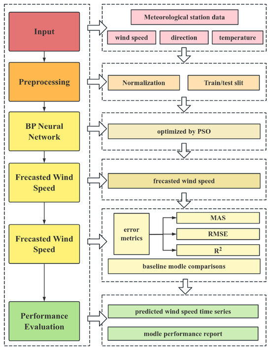
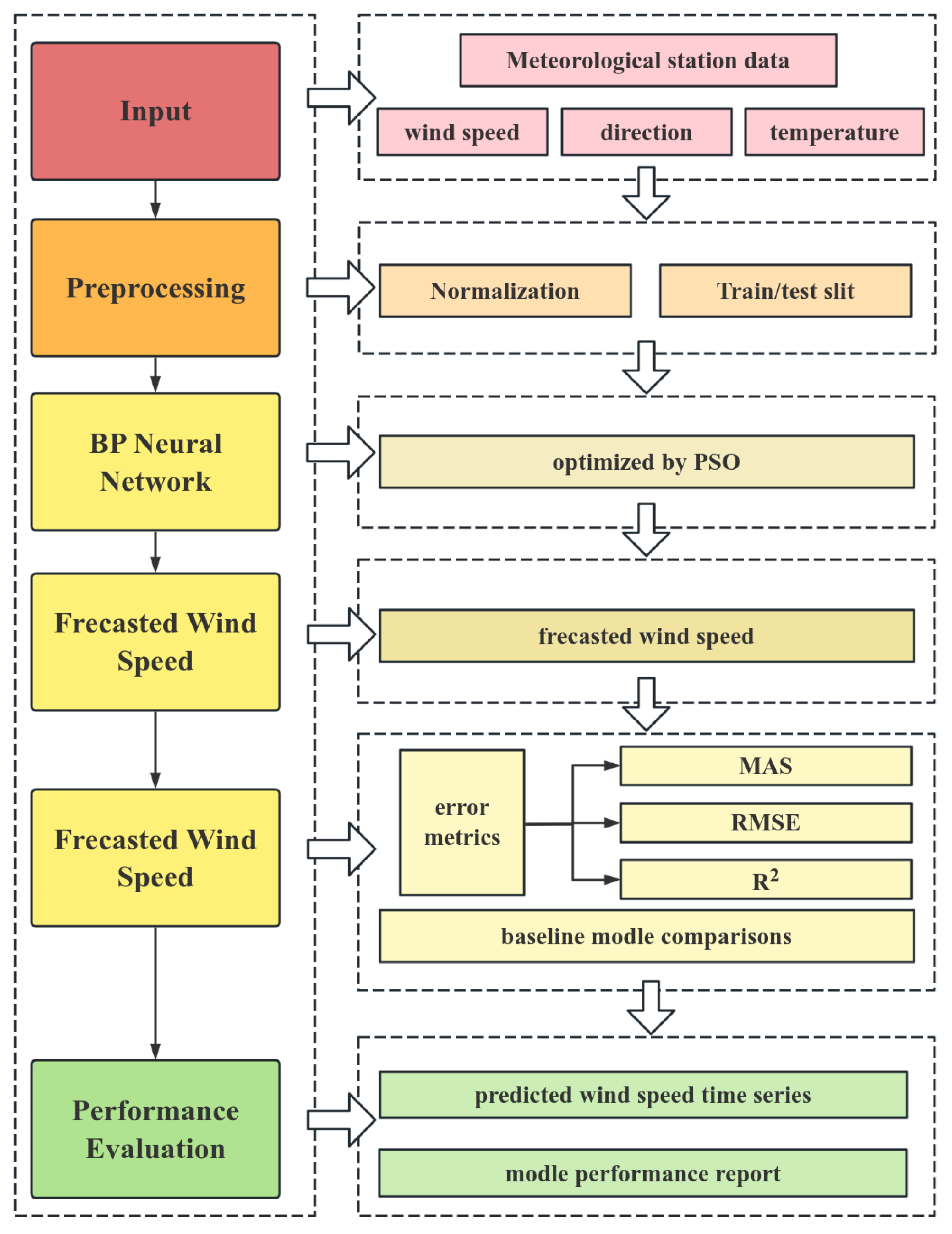
The visual overview of the basic method of this study is shown in Figure 1. Through the coordinated operation of five functional modules, the original meteorological observation data are transformed into reliable short-term wind speed predictions and quantitative performance evaluation results.

Figure 1. Framework of proposed wind resource assessment method.

The input data focus on key variables such as wind speed, wind direction and temperature collected by coastal monitoring stations. The preprocessing module for hourly recorded data is carried out and normalized to ensure the stability of model training. Then, the data are divided into a dedicated training set and a test set according to the time sequence.

The core prediction task is undertaken by the model-based prediction module. Within it, the BP neural network serves as the main prediction engine, and its structure is specifically optimized through the PSO. Choosing the BP neural network as the framework foundation is due to its mature efficacy in modeling the complex nonlinear relationships of geophysical time series (such as wind field patterns). Compared to complex deep learning models, BP architecture achieves a better balance in prediction capability, computational efficiency, and operational interpretability. The integration of the PSO is an enhancement on this basis—by globally optimizing the initial parameters (weights and biases) of the network, PSO effectively avoids the common defects of random initialization and guides the model to avoid suboptimal local minima, promoting more stable and accurate convergence during the training process. This BP-PSO hybrid model can generate the predicted wind speed sequence by processing the preprocessed historical data.

To strictly quantify the practical value of the model, the prediction results will be input into the performance evaluation module. In this stage, a set of statistical indicators including mean absolute error (MAE), root mean square error (RMSE), and Coefficient of Determination (R²) will be used to measure the deviation between the predicted wind speed and the actual observed values. To highlight the model’s advantages, we conduct a benchmark test by comparing the performance of this model with the standard baseline prediction method.

The result generation module integrates the output results of each stage of the system to form two types of core outcomes. On the one hand, it will generate the final predicted wind speed time series that can be directly used by the business; on the other hand, it will also produce a complete model performance report that includes comprehensive evaluation indicators and comparative analysis. These outcomes collectively provide crucial data input and decision-making basis for subsequent wind farm simulation, unit selection, and site comparison and selection tasks.

2.2. Backpropagation Neural Network

BP neural network, also known as error backpropagation neural network, is a multi-layer feedforward neural network that is trained using the error backpropagation algorithm. Its core lies in iteratively adjusting the connection weights and biases within the network through the gradient descent strategy to minimize the error between the network output and the expected target. This process consists of the following two key stages: forward propagation of signals and backward propagation of errors. In the forward propagation, input data are weighted and summed layer by layer through hidden layers and then transformed by a non-linear activation function (such as the Sigmoid function) to generate the output. Subsequently, the output error is calculated. Also, the error is propagated backward along the network, using the chain rule to calculate the gradient of the error with respect to each weight. The network updates all weights and biases according to the gradient information, following the direction of the fastest error decrease (negative gradient direction), and repeats this iterative process until the model converges. This mechanism endows the BP neural network with the powerful ability to automatically learn complex nonlinear mapping relationships from data. Therefore, it has become the cornerstone for solving problems such as pattern recognition, function approximation, and prediction. However, the standard BP algorithm also has some inherent flaws, including sensitivity to initial weights, easy to get stuck in local minima, slow convergence speed, and the risk of overfitting.

The BP network consists of an input layer, one or more hidden layers, and an output layer. Its operation is based on the following two fundamental processes: forward propagation and error backpropagation. For the k-th training sample, its output can be expressed as follows:

$$H_j^{(k)}=f(\sum _i{w}_{ij}^{(1)}{x}_i^{(k)}+b_j^{(1)})$$

(1)

$$O_m^{(k)}=f(\sum _j{w}_{jm}^{(2)}{H}_j^{(k)}+b_m^{(2)})$$

(2)

where $H_j^{(k)}$ represents the output of the hidden neuron j, $x_j^{(k)}$ represents the input feature of the sample, ${k O}_m^{(k)}$ represents the output of neuron m, $w_{ij}^{(1)}$, $w_{jm}^{(2)}$ are the weights between the input-hidden layer and the hidden-output layer respectively, $b_j^{(1)}$, $b_m^{(2)}$ are the biases, and $f$ is the activation function.

The squared error of sample k is given by the following formula:

$$E_k={\displaystyle \frac{1}{2}}\sum _m(O_m^{(k)}-y_m^{(k)}{)}^2$$

(3)

The total training errors are given by the following formula:

$$E=\sum _k{E}_k$$

(4)

where $y_m^{(k)}$ represents the expected (actual) output value.

Table 1 summarizes the hyperparameter settings for the BP neural network. These values are chosen based on empirical optimization and prior sensitivity analysis. As shown in Table 1, the upper and lower limits of BP parameters are set as follows: the number of neural network layers = 2, the number of neurons in the first layer is 150, the number of neurons in the second layer is 50, the learning rate is 0.000032, the batch size is 32 and the dropout rate is 0.0015. The first 80% of the training set is taken and the last 20% of the training set is taken.

Table 1. BP method setting.

Parameter	Value
number of neural network layers	2
number of neurons in the first layer	150
number of neurons in the second layer	50
learning rate	0.000032
batch size	32
dropout ratio	0.0015

The hyperparameters listed in Table 1 have been carefully selected to optimize the model performance. To determine these values, we employed the following two-stage tuning strategy: first, we explored the initial search space through grid search combined with 10-fold cross-validation on the training set. This preliminary step helped identify the potential effective ranges of key parameters (such as the number of hidden layers, the number of neurons per layer, the learning rate, and the dropout rate); subsequently, we used the particle swarm optimization algorithm to conduct a more refined global search within these ranges, aiming to minimize the validation error. The final configuration—such as an extremely low learning rate (0.000032) and a specific dropout rate (0.0015)—was proven to achieve the best balance, ensuring stable convergence during the training process while maintaining strong generalization ability on unseen data.

2.3. Particle Swarm Optimization Algorithm

The particle swarm optimization (PSO) algorithm was first proposed by Kennedy and Eberhart in 1995. It is a group intelligence optimization algorithm that simulates the social behaviors of biological groups such as bird flocks and fish schools. In PSO, each potential solution of the problem to be optimized is regarded as a “particle” in the search space. Each particle has the following two basic attributes: position (representing the solution vector) and velocity (determining the search direction and distance). During the iterative process, particles update themselves by tracking the following two extremes: one is the individual’s historical best position (pbest), which is the best solution found by the particle itself so far; the other is the group’s historically best position (gbest), which is the best solution found by the entire population so far. The velocity update formula of the particle consists of the following three parts: the inertia part (maintaining the previous movement trend), the cognitive part (learning from its own historical best), and the social part (learning from the group’s historical best). Through this information-sharing mechanism that combines individual experience with group experience, the entire particle swarm can gradually converge to the optimal solution region of the problem. The PSO is renowned for its intuitive concept, fewer parameters, simple implementation, and fast convergence speed. It is widely applied in various fields such as function optimization, neural network parameter training, and engineering design.

According to the application of PSO in the wind speed prediction model proposed by Houssein et al. [38], the calculation of the velocity of each particle can be described as follows:

$$v_i^{(t+1)}=\omega v_i^{(t)}+c_1{r}_1(p_i-x_i^{(t)})+c_2{r}_2(g_i-x_i^{(t)})$$

(5)

$$x_i^{(t+1)}=v_i^{(t+1)}+x_i^{(t)}$$

(6)

where $\omega$ is the inertia weight, $c_1$ and $c_2$ are the learning factor and cognitive coefficient and $r_1$ and $r_2$ are random numbers.

As mentioned in the previous text, the BP method has inherent limitations such as being dependent on randomly initialized data and being prone to getting stuck in local minima. To address these inherent limitations, we investigated the application of the particle swarm optimization algorithm as a meta-heuristic pre-optimizer, by exploring a set of better initial weights and biases for the backpropagation network before the traditional backpropagation begins.

In the particle swarm optimization algorithm, a group of candidate solutions called particles move in the multi-dimensional parameter space. Each particle adjusts its trajectory based on its own historically best position and the best position discovered by the entire group. This learning mechanism enables efficient exploration of the solution space. By initializing the backpropagation network using the particle swarm optimization algorithm, we effectively guide the subsequent gradient descent stage from the parameter space to a region closer to the global optimal solution, thereby achieving more stable convergence and higher prediction accuracy.

The parameter settings for controlling the dynamic search of the particle swarm optimization algorithm are as follows (Table 2 provides a summary.): the inertia weight is 0.5 to balance exploration and exploitation, the cognitive coefficient is 1.8, and the social coefficient is 2.0. The population size is 30 particles, and the number of iterations is 100. Based on the previous research and analysis methods of the research group, this configuration adopts an intermediate inertia weight, combined with numerical combinations that are close to the classical cognitive coefficient and social coefficient, in order to balance the global exploration and local exploitation capabilities, thereby ensuring the comprehensiveness of the search and the controllability of the calculation.

Table 2. PSO method settings.

Parameter	Value
$\mathsf{\omega }$	0.5
${\mathrm{c}}_1$	1.8
${\mathrm{c}}_2$	2.0

Based on the previous statements, the hybrid model of backpropagation and particle swarm optimization collaboratively utilizes the advantages of both: the particle swarm optimization algorithm conducts a global coarse-grained search to obtain a favorable starting point, followed by the backpropagation network performing local fine-grained optimization through gradient descent. This collaborative strategy enhances the reliability and performance of the model, making it a robust tool for short-term wind speed prediction under practical operating conditions.

2.4. Probabilistic Forecasting for Grid Integration

Wind speed, being a stochastic meteorological variable, carries inherent uncertainty. For a wind speed prediction model to be useful in grid operation—such as for unit commitment, economic dispatch, or reserve planning—it must not only provide a point forecast but also quantify the associated uncertainty. A point forecast alone is insufficient for risk-averse decision-making in power systems [39]. Therefore, we extend our deterministic BP-PSO model to a probabilistic forecasting framework by constructing prediction intervals (PIs).

Following the methodology established by Gal & Ghahramani (2016) [40] and Khosravi et al. (2011) [41], we employ the Monte Carlo Dropout (MC-Dropout) method to generate prediction intervals. MC-Dropout approximates Bayesian inference by applying dropout during both training and testing phases. For a given input xx, the predictive distribution is obtained by performing T stochastic forward passes:

$${\left\{{\widehat{y}}_t\right\}}_{t=1}^T={\left\{f_{{\theta }_i}\left(x\right)\right\}}_{t=1}^T$$

(7)

where $f_{{\theta }_i}\left(x\right)$ denotes the network output with dropout applied.

The mean of these T predictions serves as the final point forecast:

$${\widehat{y}}_m={\displaystyle \frac{1}{T}}\sum _{t=1}^T\widehat{y_t}$$

(8)

The $100(1-\alpha )\%$ prediction interval is constructed from the empirical quantiles of the predictive distribution:

$${PI}_{1-\alpha }=\left[{\widehat{y}}_{(\alpha /2)},{\widehat{y}}_{(1-\alpha /2)}\right]$$

(9)

where ${\widehat{y}}_{(\alpha /2)}$ and ${\widehat{y}}_{(1-\alpha /2)}$ are the α/2 and 1 − α/2 quantiles, respectively. In this study, we construct 80% prediction intervals (α = 0.2).

The quality of the PIs is evaluated using two key metrics:

1. Prediction Interval Coverage Probability (PICP)

$$\mathrm{P}\mathrm{I}\mathrm{C}\mathrm{P}={\displaystyle \frac{1}{N}}\sum _{i=1}^N\mathbb{I}\left\{y_i\in {\mathrm{P}\mathrm{I}}_i\right\}$$

(10)

where $\mathbb{I}\left\{y_i\in {\mathrm{P}\mathrm{I}}_i\right\}$ is the indicator function, and N is the number of test samples. A higher PICP (closer to the nominal confidence level, e.g., 80%) indicates better reliability.

2. Mean Prediction Interval Width (MPIW):

$$MPIW={\displaystyle \frac{1}{N}}\sum _{i=1}^N\left({\widehat{y}}_{i,(1-\alpha /2)}-{\widehat{y}}_{i,(\alpha /2)}\right)$$

(11)

A narrower MPIW, for a given PICP, indicates a more informative and sharp forecast.

The importance of such probabilistic forecasts for power system operation has been emphasized by Pinson & Kariniotakis (2010) [39], who demonstrate that prediction intervals enable grid operators to make informed decisions about reserve allocation and risk management.

3. Case Study

In order to put the BP-PSO hybrid prediction model constructed in the previous section to empirical verification, this study selected the typical coastal site Lao Hu Tan (LHT) as the specific case analysis object. Our aim is to systematically verify the applicability and prediction accuracy of the model in the actual wind field environment, thereby providing reliable data support and decision-making references for wind resource assessment and wind power operation management in coastal areas.

The research began by obtaining hourly wind speed observation data for the LHT site from public platforms such as the National Ocean Science Data Center. A continuous time series covering different seasons and meteorological conditions was constructed. This dataset not only reflects the annual variation characteristics of the regional wind field but also contains inter-annual fluctuation information, providing sufficient climate representativeness for model training. During the data preprocessing stage, we cleaned, denoised, and normalized the original sequence to enhance the stability and convergence efficiency of the subsequent modeling.

Based on this, the particle swarm optimization (PSO) algorithm is introduced to conduct global optimization of the initial weights and biases of the BP neural network. This step helps to avoid the model getting stuck in local optimum and significantly accelerates the training convergence speed. The optimized parameters will be used as the initialization configuration of the BP network, and then a multi-layer feedforward network based on error backpropagation will be constructed, specifically for learning the complex nonlinear temporal dependencies in the wind speed sequence.

To comprehensively evaluate the performance of the proposed BP-PSO framework, this study employed the following two modeling strategies: one is global modeling based on complete multi-year data, and the other is detailed modeling tailored to different seasonal characteristics. Specifically, we used the data from January 2020 to December 2022, spanning a total of three years, as both the training set for the multi-year model and the seasonal models, to ensure a fair comparison between the two; the data from January 2023 to July 2023 were retained as an independent test set to verify the generalization ability and prediction accuracy of the model.

In seasonal modeling, the training data is further divided into the following four seasonal subsets based on calendar months: spring (March–May), summer (June–August), autumn (September–November), and winter (December to February of the following year). An independent BP-PSO model is trained for each season, and the data from the corresponding period in 2023 are used for evaluation. It is worth noting that since data after July 2023 are temporarily unavailable, this analysis only validates the prediction results for spring (March–May) and summer (June–July), and the predictions for autumn and winter have not been included in this round of evaluation.

Ultimately, this study will conduct simulation and multi-angle prediction analysis of wind speed at the LHT site using the PSO-BP combined framework. We not only focus on the accuracy and stability of the model in short-term forecasting, but also systematically examine its response ability to seasonal fluctuations, thereby providing scientific and practical technical basis for the real-time scheduling, operation maintenance, and medium- and long-term energy planning of wind farms in this region.

3.1. Data and Site Description

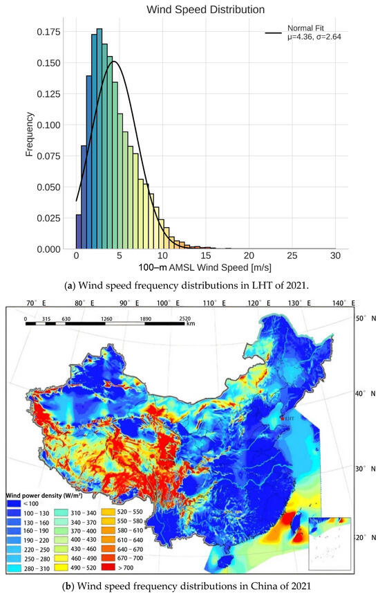
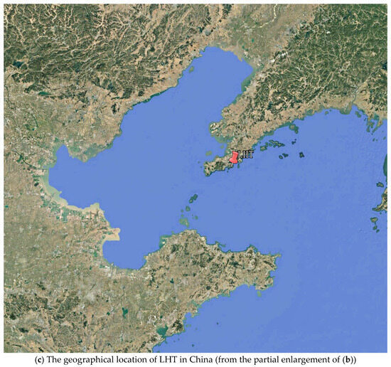
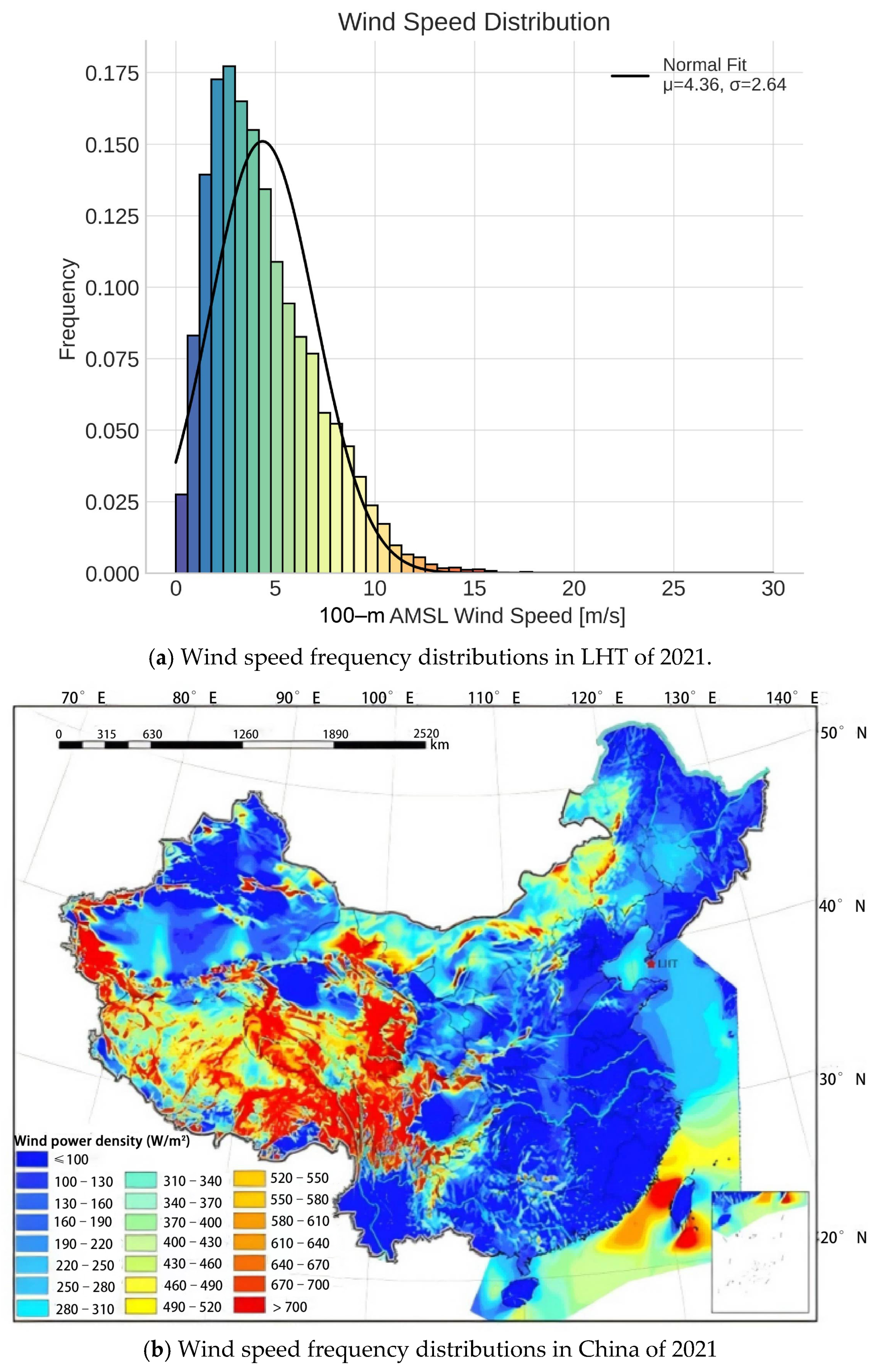
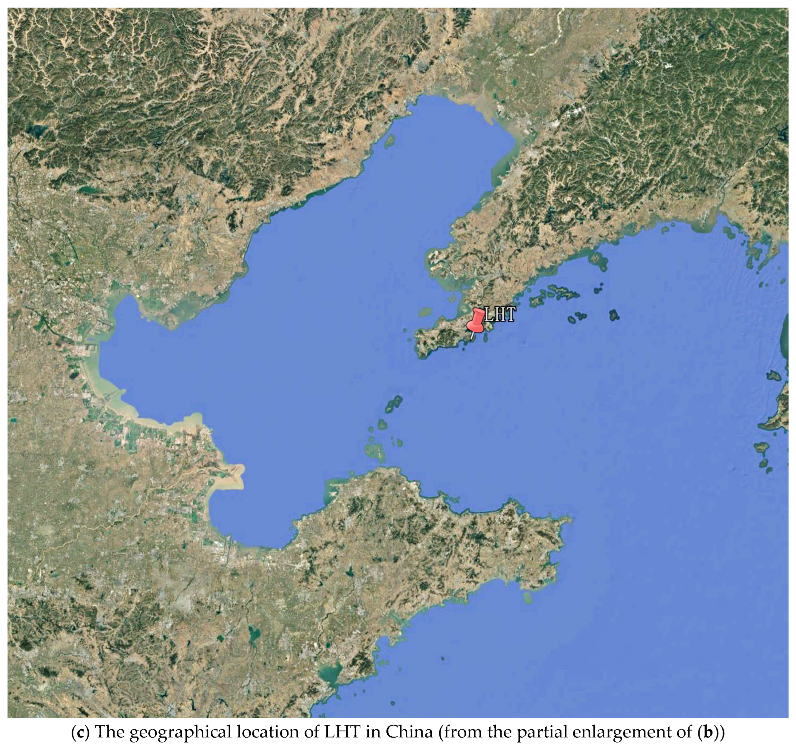
The average sea level height wind speed probability distribution of LHT and the wind energy density under different terrains in China are shown in Figure 2a (from Jiang et al.) [32] Figure 2b and Figure 2c respectively.

Figure 2. AMSL wind speed probability (LHT) and wind energy density over different terrains in China.

As shown in Figure 2a, the probability distribution map of average sea level height (AMSL) wind speed is plotted based on the field measurement data. The normalized histogram presents the probability density function (the color scale ranges from blue to red, representing the increase in wind speed, and the overlaid black curve shows the fitted normal distribution). Through relevant calculations, the average wind speed is determined to be 4.36 m/s, and the standard deviation is 2.64 m/s.

The distribution is right-skewed, indicating a greater frequency of lower wind speeds and fewer high wind events. The modal wind speed (i.e., the most frequent bin) lies between 2.5 and 4.5 m/s, which aligns with commonly observed daily average wind conditions.

The current figure represents the aggregated annual data; wind speeds tended to peak during spring and early summer (April–July), while lower values were generally recorded during autumn months (October–November). Monthly breakdowns also revealed a bimodal seasonal trend, which is consistent with mesoscale circulation patterns and regional climatology.

LHT (located in Liaoning Province, China, at longitude 121.7 degrees east and latitude 38.9 degrees north; the red dots in the picture have been marked) is situated in China. This study utilized hourly wind speed data from a meteorological station in the coastal area in 2021. Figure 2b,c show the location of LHT on the Chinese map and the wind energy density (W/m²) of LHT under different terrain conditions in China. LHT is located in the eastern coastal area of China. Also, it is clearly visible that the area where LHT is situated has a high wind energy density, containing abundant exploitable wind power resources, and can serve as a representative of offshore wind power resources utilization in the eastern coastal areas of China. This region can also better validate the advantages of the BP-PSO model in this study, which will help verify and demonstrate the practicality and stability of this model in wind energy prediction in the eastern coastal areas of China.

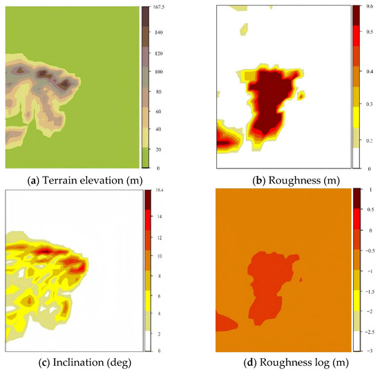
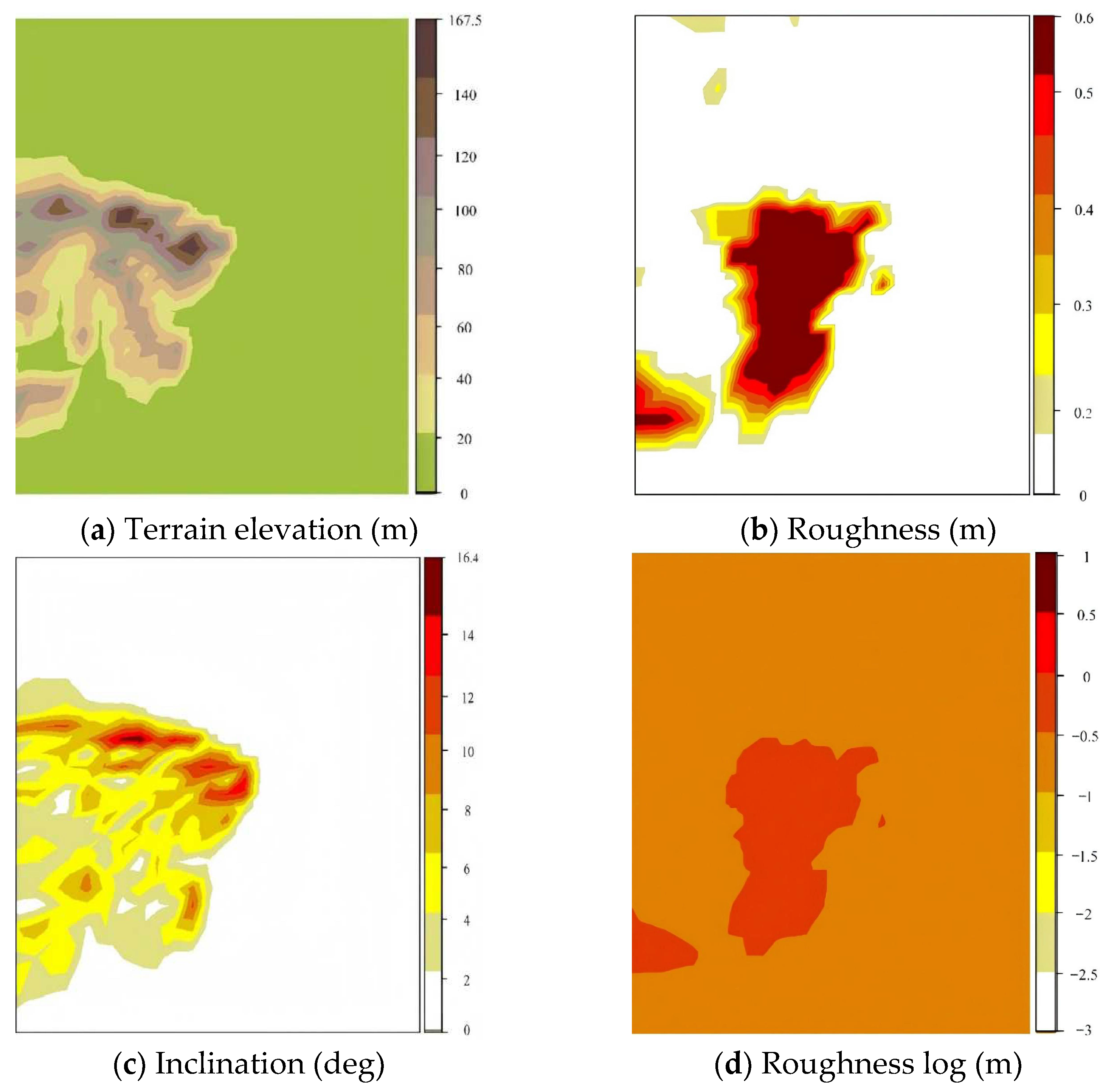
As shown in Figure 3, it comprehensively presents the key topographical and surface characteristic parameters of the LHT wind farm. Figure 3a is elevation of the wind farm, (b) is a roughness height picture which indicates roughness height, (c) is the inclination in the farm and picture (d) is roughness log in the site LHT.

Figure 3. Key terrain and surface parameters of the LHT wind farm.

Among them, the elevation distribution is the basis for influencing the atmospheric boundary layer flow and local acceleration effect; the height of surface roughness directly determines the wind shear strength and turbulence characteristics in the near-ground layer; the field area inclination (slope) will change the local wind speed and direction through terrain uplift or channel effect, while the logarithm of roughness is a parameter obtained by logarithmically processing the height of roughness, and is widely used as an input in wind profile models.

3.2. Multi-Year BP-PSO Forecasting Performance

This long-term model was trained using complete and continuous hourly wind speed data from January 2020 to December 2022. This three-year dataset covers multiple complete annual cycles, with the aim of allowing the model to encounter and learn the typical patterns of wind fields, seasonal fluctuations, and various extreme event characteristics that may recur in different years.

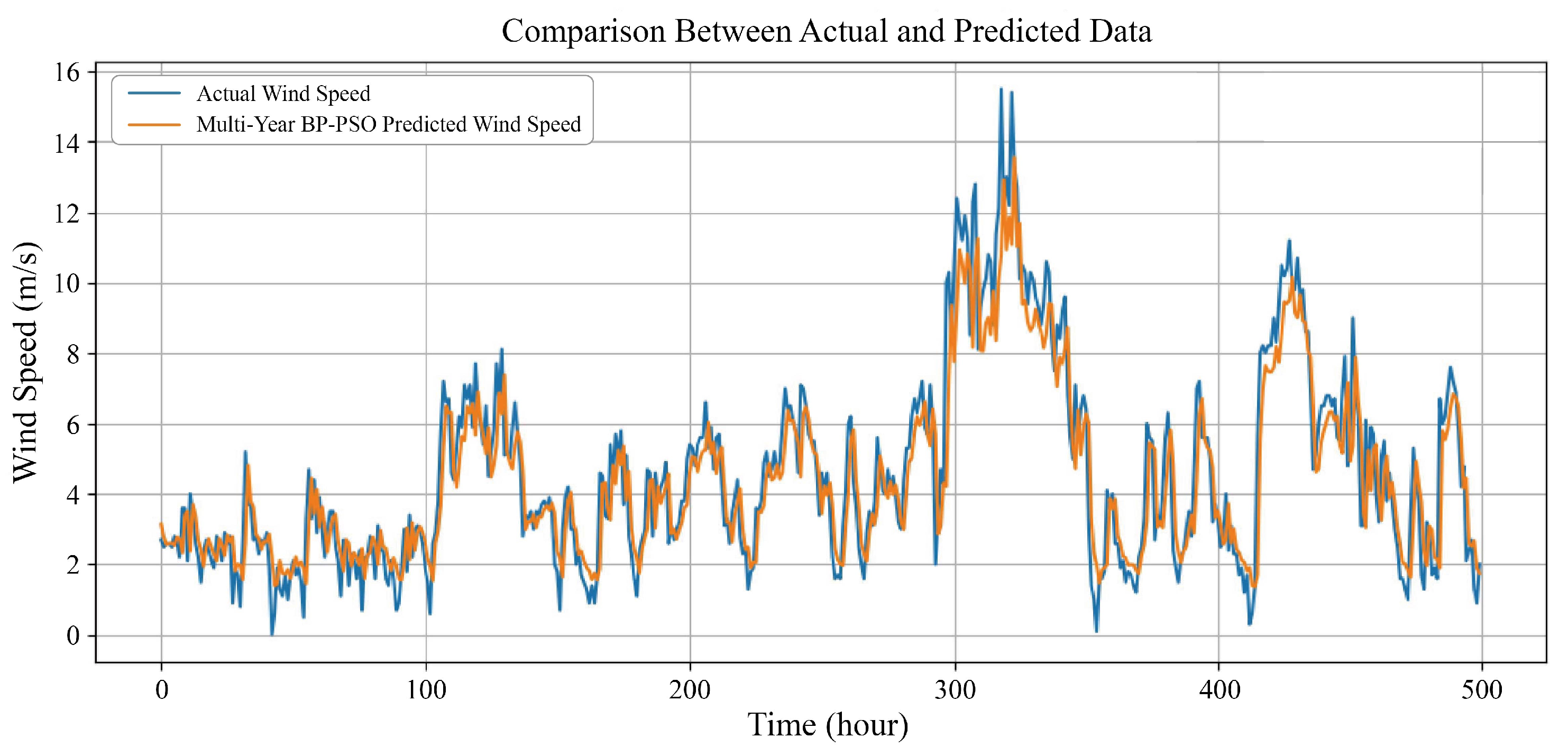
The trained model was applied to the independent test period from January to July 2023. The comparison of the predicted results with the actual observations is shown in Figure 4.

Figure 4. Multi-year forecast and comparation.

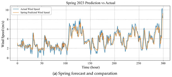
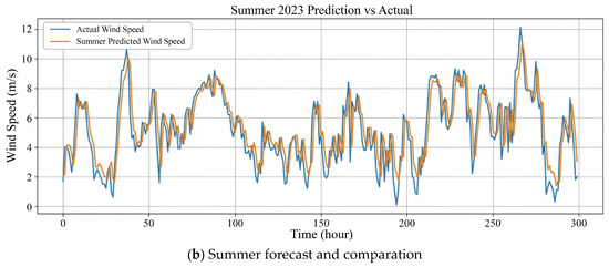
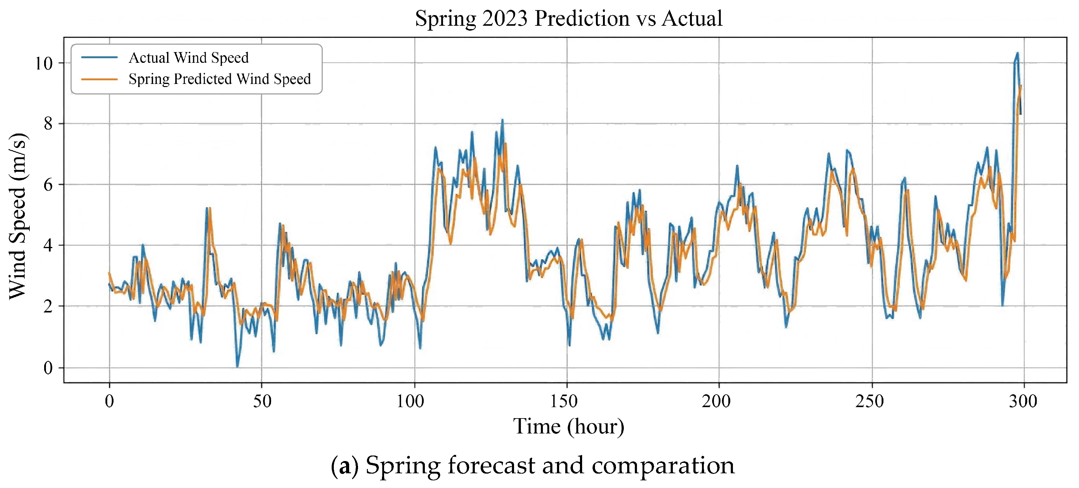
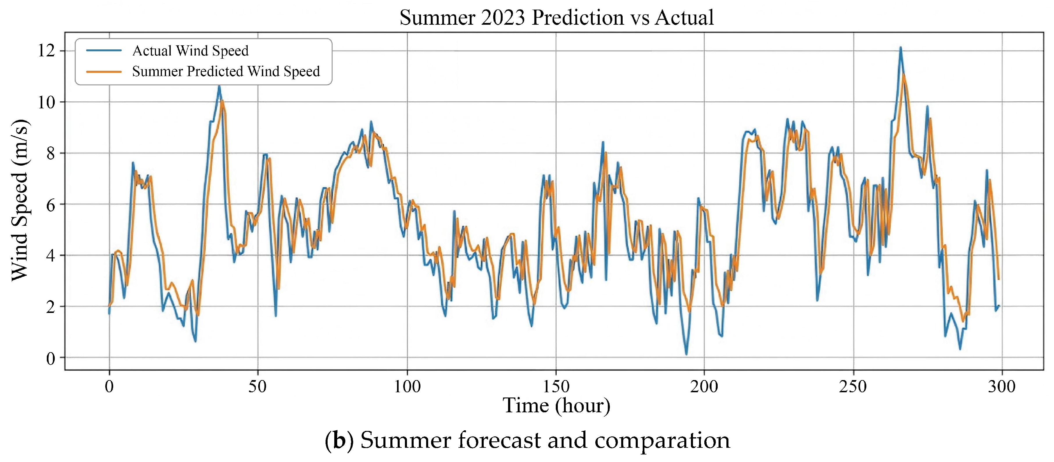
The horizontal axis (x-axis) is time index, and the vertical axis (y-axis) is wind speed (m/s). The blue “Actual” curve represents the actual wind speed, while the yellow one represents the simulated prediction result curve. The same applies to Figure 5 and Figure 6 in the following text.

Figure 5. Spring and summer forecast and comparation.

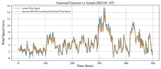
Figure 6. Combined seasonal forecast and comparation.

The visualization results indicate that the predicted curve output by the model has a high degree of consistency with the actual wind speed curve in terms of overall shape and change direction. The model not only reproduced the daily fluctuation trend of wind speed but also showed timely following and reflection for several significant wind speed peaks that occurred during the test period. This initially indicates that the prediction output of this model is stable and reasonable when faced with new and unseen data.

The quantitative calculation of prediction errors provides objective evidence for the model’s performance. During the entire seven-month testing period, the model’s RMSE was 1.235 and the MAE was 0.924. These two key error indicators were at a relatively low level, quantitatively demonstrating that the overall deviation between the model’s predicted values and the actual observations was small. An important observation is that although the testing period spanned from the end of winter to the middle of summer, the model maintained consistent prediction accuracy throughout the period, without experiencing a sudden deterioration in performance in any particular month of the season. These results collectively show that the global model trained based on complete data over many years demonstrates reliable robustness in cross-seasonal prediction tasks. Without any special design for any season, it achieved a prediction effect that balances accuracy and consistency.

3.3. Benchmark Model Comparative Analysis

To evaluate and demonstrate the advantages of our proposed BP-PSO model in this research, we compared the performance results with some widely recognized baseline methods, including LSTM, ARIMA, and persistence models. At the same time, we noticed that previous members of the research group had certain research foundations in this field. We compared the results with the model and benchmark study by Jiang et al. (2025) [32]. All baseline models were trained and tested using the same dataset (training data from 2020 to 2022, and test data from January to July 2023) and the same short-term prediction configuration (24 h input, 1 h output) as our model.

The results in Table 3 show that the proposed BP-PSO model achieved the lowest root mean square error (RMSE) and mean absolute error (MAE) among all the compared methods. Specifically, its RMSE metric was improved by approximately 12% compared to the LSTM model, highlighting the effectiveness of the particle swarm optimization algorithm in alleviating the problem of BP network getting trapped in local minima, thereby obtaining a solution closer to the global optimum. More importantly, our model demonstrated a significant improvement compared to the benchmark result of Jiang et al. (2025) [32] (the RMSE decreased from 1.27 to 1.235), confirming the optimization effectiveness of the modeling method.

Table 3. Performance comparison of different models at LHT site.

Model	RMSE (m/s)	MAE (m/s)	R2
BP-PSO model (this work)	1.235	0.924	0.89
Jiang et al.—multi-year model	1.270	0.932	0.70
LSTM	1.401	1.078	0.84
ARIMA	1.572	1.232	0.79
Persistence models	1.673	1.278	0.75

The proposed model significantly outperforms the traditional ARIMA and persistent baseline models, with a substantial reduction in the RMSE value. This finding confirms the necessity of using nonlinear models such as BP-PSO to capture the complex dynamic characteristics of wind speed. These comparative results provide indirect evidence that the short-term wind speed prediction framework we proposed for the eastern coastal stations in China offers an excellent solution.

3.4. Seasonal BP-PSO Forecasting and Comparative Analysis

To evaluate the effect of seasonal decomposition on forecast accuracy, BP-PSO models were individually trained for spring, summer, autumn, and winter using 2020–2022 data. Limited data availability restricts the presented analysis to spring and summer outcomes (Figure 5).

The spring 2023 seasonal model shows strong correspondence to observed wind speeds, especially under moderately varying conditions (Figure 5a). Its performance, quantified by an RMSE of 1.243 and an MAE of 0.924, is comparable to the integrated multi-year model.

During the summer of 2023, this model exhibited a significant deviation from the measured data during the stage of sudden wind speed changes (Figure 5b), which might be attributed to the occurrence of strong convective activities and complex turbulence. The RMSE rose to 1.324, while the MAE remained stable at 1.010. The increase in the RMSE coexisted with the stability of the MAE, indicating that the model occasionally made errors in predicting short-term peak intensities.

3.5. Error Analysis and Interpretation

By integrating the prediction results of each individual seasonal model, we synthesized a comprehensive seasonal forecast result based on the original results and reconstructed the wind speed trajectories for certain periods of the year (Figure 6). Although specialized seasonal training was supposed to enhance the model performance, the RMSE of the combined model was 1.255, slightly higher than that of the multi-year model (1.235). This minor difference indicates that the advantages brought by specialized seasons may be offset by the technical challenges of seamlessly integrating discrete seasonal predictions.

To better understand the predictive behavior of the model, we will now compare and interpret the RMSE values of the long-term model and the seasonal models (spring, summer, and the combined model).

The multi-year BP-PSO model, trained on the complete data set from January 2020 to December 2022, achieved the lowest RMSE of 1.235 when evaluated over the test period from January to July 2023. This confirms the overall reliability and robustness of the global model across different seasonal patterns. In contrast with each other, the spring and summer seasonal models respectively yielded RMSE values of 1.243 and 1.324. The combined seasonal model, which concatenates predictions from available seasons, resulted in an intermediate RMSE of 1.255.

Interestingly, although the seasonal model was designed to capture the dynamic characteristics of specific seasons, its performance did not surpass that of the multi-year comprehensive model. This counter-intuitive phenomenon may be caused by multiple factors: from the perspective of sample size changes, the training sample size of the seasonal model has significantly decreased (only one quarter of the complete training set), which limits its generalization ability; from the perspective of seasonal differences, although all models adopt the same BP-PSO network structure, the wind speed distribution in different seasons shows significant differences. If the hyperparameters are not adjusted for specific seasons, it may lead to underfitting in some seasons (such as summer) and overfitting in other seasons. The third possible factor is that the multi-year model benefits from continuous and complete time series data, while the seasonal model lacks the contextual information provided by long-term time patterns, which results in this problem from an intuitive perspective. The dynamic characteristics of specific seasons are actually lower than those of the multi-year comprehensive model.

The performance differences between the spring and autumn models are also worthy of attention. The spring model shows a lower RMSE (1.243), close to the level of the global model, which is likely due to the stable atmospheric conditions and mild wind speed changes in this season. In contrast, the RMSE of the summer model is the highest (1.324), attributed to frequent large-amplitude fluctuations, convective activities, and extreme events such as thunderstorms and typhoons—these complex phenomena are difficult to accurately model using a simple feedforward structure.

Furthermore, the combined seasonal model has a structural defect of prediction discontinuity. Since each seasonal model is trained independently, during the seasonal transition (such as from May to June), it may cause inconsistency in the prediction sequence. This discontinuity accumulates and combines with the seasonal modeling errors, which partly explains why the RMSE (1.255) of the combined seasonal model is higher than that of the multi-year model.

3.6. Probabilistic Forecasting Results and Grid Integration Assessment

We applied the MC-Dropout probability prediction framework to the long-term BP-PSO model. The results during the test period (from January to July 2023) showed that the long-term BP-PSO model achieved a PICP (prediction interval coverage probability) of 81.2%, which was very close to the nominal confidence level of 80%, indicating that the constructed prediction intervals had good calibration. The average width of these intervals $MPIW=1.38 \mathrm{m}/\mathrm{s}$ provided quantifiable uncertainty measurement indicators for grid operators.

This result is of practical significance for grid operation. For instance, if the BP-PSO model predicts a wind speed of 8 m/s (corresponding to, say, 50% of a wind turbine’s rated power), the P10–P90 interval of [6.8, 9.4] m/s indicates that the actual power output could range from 30% to 70% of the rated power. Knowing this, a grid operator can confidently schedule a reserve capacity (e.g., 70% of rated power) to maintain grid stability. This is a significant advancement from simply relying on a point forecast, which could lead to either over-provisioning (wasteful) or under-provisioning (risky) of reserves. This probabilistic output, as argued by Pinson & Kariniotakis (2010) [39] and Xiong (2023) [29], is a critical step towards integrating high-penetration wind power into the grid.

4. Conclusions and Discussion

This section compares global forecasting tools with Chinese regional analysis products based on publicly available data from operational systems and reanalysis datasets. WINDY.com visualizes outputs from major global numerical weather prediction (NWP) models like GFS and ECMWF. These models solve atmospheric physics equations and are updated through data assimilation, providing essential global coverage. However, their typical resolution (9–30 km) often cannot resolve local terrain effects such as surface roughness or coastal features that significantly influence site-specific wind speeds. Therefore, direct NWP output may show systematic biases for single-point forecasts.

China provides high-resolution regional products like CLDAS, which generates hourly 10 m wind speed fields at 0.0625° resolution. Studies report CLDAS achieves about 0.83 m/s RMSE for wind speed in China, a reliable regional benchmark. Our multi-year BP-PSO model achieved 1.235 m/s RMSE on a 2023 test set. While higher than CLDAS error, both methods have trade-offs. The BP-PSO model trains solely on historical site data, learning local climate patterns that NWP models miss, making it well-suited for specific locations. It enables near real-time predictions for applications like turbine control. However, its local data dependence limits transferability, and its data-driven nature may struggle with unprecedented extremes that NWP can simulate physically.

Exploring complementarity between these tools is worthwhile. Global models provide large-scale context while site-specific machine learning corrects local biases. This points toward hybrid approaches: using NWP outputs as inputs to BP-PSO frameworks, combining physical principles with data-driven refinement. Such integration could improve both generalization and extreme event forecasting.

This study reaches a clear conclusion. Under the BP-PSO framework, the global model trained on complete multi-year data outperforms seasonally divided models. This suggests long-term continuity and cross-season patterns are more valuable than seasonal specialization for this task. Seasonal modeling did not show expected advantages here. When using decomposition strategies like seasonal splitting, we must weigh benefits against costs. Although splitting may help models focus on specific periods, it loses long-term dependencies and reduces training data, potentially limiting generalization. Here, these drawbacks outweighed seasonal benefits. Future research could test whether seasonal modeling becomes advantageous with larger datasets or in different climate zones. Another direction is hybrid modeling: using global models for baseline patterns, then fine-tuning for seasons or extremes. This study shows both data consistency and model complexity matter for accurate wind speed prediction.

In conclusion, this study successfully developed and validated a PSOoptimized BP neural network for short-term offshore wind speed forecasting. While the core algorithm is well-established, the methodological contributions lie in the novel “data-to-physics” integration framework, the systematic comparison of seasonal versus multi-year modeling strategies under data-limited conditions, and the extension to a probabilistic forecasting framework. The multi-year model demonstrated superior performance, achieving an RMSE of 1.235 m/s and an MAE of 0.924 m/s, outperforming conventional baselines like LSTM and ARIMA, and compared to the baseline results of the previous research group’s work, there is a significant improvement.

Most importantly, by generating well-calibrated prediction intervals (PICP = 81.2%) using MC-Dropout, the model moves beyond simple point forecasting to provide actionable uncertainty information for grid operation. This addresses a key requirement for integrating high-penetration wind power into the electricity grid. Looking forward, based on BP-PSO predictions, we plan CFD simulations for wind resource and wake assessment using WindSim under steady conditions with high-resolution DEM data for terrain parameters. Predicted wind speed sequences will drive logarithmic wind profiles. For wake modeling, the Jensen model will estimate energy losses efficiently, balancing accuracy and practicality for iterative analysis. This approach will support turbine selection, layout optimization, and annual energy yield forecasts.

References

- Asif, M.; Muneer, T. Energy supply, its demand and security issues for developed and emerging economies. Renew. Sustain. Energy Rev. 2007, 11, 1388–1413. [Google Scholar] [CrossRef] [Scilit]
- Asadi, E.; Sadjadi, S.J. Optimization methods applied to renewable and sustainable energy: A review. Uncertain Supply Chain Manag. 2017, 5, 1–26. [Google Scholar] [CrossRef] [Scilit]
- Desalegn, B.; Gebeyehu, D.; Tamrat, B.; Tadiwose, T.; Lata, A. Onshore versus offshore wind power trends and recent study practices in modeling of wind turbines’ life-cycle impact assessments. Clean. Eng. Technol. 2023, 17, 100691. [Google Scholar] [CrossRef] [Scilit]
- Li, J.; Wang, G.; Li, Z.; Yang, S.; Chong, W.T.; Xiang, X. A review on development of offshore wind energy conversion system. Int. J. Energy Res. 2020, 44, 9283–9297. [Google Scholar] [CrossRef] [Scilit]
- Global Wind Energy Council. Global Wind Report 2025; GWEC: Lisbon, Portugal, 2025. [Google Scholar]
- REN21. Renewables 2023 Global Status Report; REN21 Secretariat: Paris, France, 2023. [Google Scholar]
- Ahmed, S.D.; Al-Ismail, F.S.M.; Shafiullah, M.; Al-Sulaiman, F.A.; El-Amin, I.M. Grid integration challenges of wind energy: A review. IEEE Access 2020, 8, 10857–10878. [Google Scholar] [CrossRef] [Scilit]
- Gode, P.R.; Aspelund, A. Addressing heterogeneity in the development of circular economy strategies in the offshore wind industry: A review. Heliyon 2024, 10, e39577. [Google Scholar] [CrossRef] [Scilit]
- Tominaga, Y. CFD simulations of turbulent flow and dispersion in built environment: A perspective review. J. Wind Eng. Ind. Aerodyn. 2024, 249, 105741. [Google Scholar] [CrossRef] [Scilit]
- Barile, D.A.; Sosa, R.; Aubrun, S.; Otero, A.D. Novel CFD approach for simulation of an ABL wind tunnel flow: Validation and application to a FOWT model. Wind Energy Sci. Discuss. 2025. preprint. [Google Scholar] [CrossRef] [Scilit]
- Khedr, A.; Castellani, F. Critical issues in the moving reference frame CFD simulation of small horizontal axis wind turbines. Energy Convers. Manag. X 2024, 22, 100551. [Google Scholar] [CrossRef] [Scilit]
- Zhang, Z.; Mao, Y.; Su, X.; Yuan, X. Adjoint-Based Boundary Condition Sensitivity Analysis. AIAA J. 2022, 60, 3517–3527. [Google Scholar] [CrossRef] [Scilit]
- Liu, Z.; Guo, H.; Zhang, Y.; Zuo, Z. A Comprehensive Review of Wind Power Prediction Based on Machine Learning: Models, Applications, and Challenges. Energies 2025, 18, 350. [Google Scholar] [CrossRef] [Scilit]
- Geng, D.; Zhang, Y.; Zhang, Y.; Qu, X.; Li, L. A hybrid model based on CapSA-VMD-ResNet-GRU-attention mechanism for ultra-short-term and short-term wind speed prediction. Renew. Energy 2025, 240, 122191. [Google Scholar] [CrossRef] [Scilit]
- Harbola, S.; Coors, V. Comparative Analysis of LSTM, RF and SVM Architectures for Predicting Wind Nature for Smart City Planning. ISPRS Ann. Photogramm. Remote Sens. Spat. Inf. Sci. 2019, IV-4/W9, 65–70. [Google Scholar] [CrossRef] [Scilit]
- Li, X.; Li, K.; Shen, S.; Tian, Y. Exploring Time Series Models for Wind Speed Forecasting: A Comparative Analysis. Energies 2023, 16, 7785. [Google Scholar] [CrossRef] [Scilit]
- Tjøstheim, D. Selected Topics in Time Series Forecasting: Statistical Models vs. Machine Learning. Entropy 2025, 27, 279. [Google Scholar] [CrossRef] [Scilit]
- Hajirahimi, Z.; Khashei, M. Hybrid structures in time series modeling and forecasting: A review. Eng. Appl. Artif. Intell. 2019, 86, 83–106. [Google Scholar] [CrossRef] [Scilit]
- Zhang, Y.; Wang, J.; Lu, H. Short-term wind speed forecasting based on LSTM networks optimized by Bayesian inference. Energy Convers. Manag. 2021, 239, 114221. [Google Scholar] [CrossRef] [Scilit]
- Yang, Y.; Lou, H.; Wu, J.; Zhang, S.; Gao, S. A survey on wind power forecasting with machine learning approaches. Neural Comput. Appl. 2024, 36, 12753–12773. [Google Scholar] [CrossRef] [Scilit]
- Ilardi, D. Computationally Aware Surrogate Models for the Hydrodynamic Response Characterisation of Floating Spar-Type Offshore Wind Turbine. IEEE Access 2024, 12, 6494–6517. [Google Scholar] [CrossRef] [Scilit]
- Walker, J.M. Data-Driven Models for Yacht Hull Resistance Optimization: Exploring Geometric Parameters Beyond the Boundaries of the Delft Systematic Yacht Hull Series. IEEE Access 2024, 12, 76102–76120. [Google Scholar] [CrossRef] [Scilit]
- Hanifi, S.; Lotfian, S.; Zare-Behtash, H.; Cammarano, A. Offshore Wind Power Forecasting—A New Hyperparameter Optimisation Algorithm for Deep Learning Models. Energies 2022, 15, 6919. [Google Scholar] [CrossRef] [Scilit]
- Zhang, K.S.; Qiao, H.L.; Wang, P.H.; Du, Y.Q.; Han, Z.H. Exploration of Efficient Hyperparameters Adaption of Support Vector Regression for Aerodynamic Design. ICAS Proceedings. 2024. Available online: http://pure.nwpu.edu.cn/zh/publications/exploration-of-efficient-hyperparameters-adaption-of-support-vect/ (accessed on 5 March 2026).
- Wang, H.; Tan, Z.; Liang, Y.; Li, F.; Zhang, Z.; Ju, L. A novel multi-layer stacking ensemble wind power prediction model under Tensorflow deep learning framework considering feature enhancement and data hierarchy processing. Energy 2024, 286, 129409. [Google Scholar] [CrossRef] [Scilit]
- Taha, A.; Nazih, N.; Makeen, P. Wind speed prediction based on variational mode decomposition and advanced machine learning models in zaafarana, Egypt. Sci. Rep. 2025, 15, 15599. [Google Scholar] [CrossRef] [Scilit] [PubMed]
- AbdElkader, A.G.; ZainEldin, H.; Saafan, M.M. Optimizing wind power forecasting with RNN-LSTM models through grid search cross-validation. Sustain. Comput. Inform. Syst. 2025, 45, 101054. [Google Scholar] [CrossRef] [Scilit]
- Ren, C.; An, N.; Wang, J.; Li, L.; Hu, B.; Shang, D. Optimal parameters selection for BP neural network based on particle swarm optimization: A case study of wind speed forecasting. Knowl.-Based Syst. 2014, 56, 226–239. [Google Scholar] [CrossRef] [Scilit]
- Xiong, M. Probabilistic Wind Gust Forecasting during the 2022 Beijing Winter Olympics. J. Meteorol. Res. 2023, 37, 743–756. [Google Scholar] [CrossRef] [Scilit]
- Tian, R.; Kou, P.; Zhang, Y.; Mei, M.; Zhang, Z.; Liang, D. Residual-connected physics-informed neural network for anti-noise wind field reconstruction. Appl. Energy 2024, 357, 122439. [Google Scholar] [CrossRef] [Scilit]
- Zhao, S.Y.; Jin, J.Y.; Han, P.F. Numerical simulation of offshore wind energy resources based on CFD. Acta Energiae Solaris Sin. 2025, 46, 378–385. [Google Scholar] [CrossRef]
- Jiang, S.J.; Jin, J.Y. Offshore wind energy assessment considering different wake effect models. In Proceedings of the 2023 2nd Asian Conference on Frontiers of Power and Energy (ACFPE), Chengdu, China, 27–29 October 2023; pp. 655–659. [Google Scholar] [CrossRef] [Scilit]
- Dai, S.; Song, Y.; Zhu, Y.; Ye, M.; Wang, H.; Wen, J.-F. Recalibration of IEC Turbulence Model Based on Field Observations. J. Mar. Sci. Eng. 2025, 13, 1957. [Google Scholar] [CrossRef] [Scilit]
- García Márquez, F.P.; Peinado Gonzalo, A. A Comprehensive Review of Artificial Intelligence and Wind Energy. Arch. Comput. Methods Eng. 2022, 29, 2935–2958. [Google Scholar] [CrossRef] [Scilit]
- Wang, C.-H.; Zhao, Q.; Tian, R. Short-Term Wind Power Prediction Based on a Hybrid Markov-Based PSO-BP Neural Network. Energies 2023, 16, 4282. [Google Scholar] [CrossRef] [Scilit]
- Ahmadi, M.; Khashei, M. Current status of hybrid structures in wind forecasting. Eng. Appl. Artif. Intell. 2021, 99, 104133. [Google Scholar] [CrossRef] [Scilit]
- Sweetman, B.; Dai, S. Transformation of Wind Turbine Power Curves Using the Statistics of the Wind Process. IEEE Trans. Sustain. Energy 2021, 12, 2053–2061. [Google Scholar] [CrossRef] [Scilit]
- Houssein, E.H. Particle Swarm Optimization-Enhanced Twin Support Vector Regression for Wind Speed Forecasting. J. Intell. Syst. 2019, 28, 905–914. [Google Scholar] [CrossRef] [Scilit]
- Pinson, P.; Kariniotakis, G. Conditional Prediction Intervals of Wind Power Generation. IEEE Trans. Power Syst. 2010, 25, 1845–1856. [Google Scholar] [CrossRef] [Scilit]
- Gal, Y.; Ghahramani, Z. Dropout as a Bayesian Approximation: Representing Model Uncertainty in Deep Learning. Int. Conf. Mach. Learn. 2016, 48, 1050–1059. Available online: https://proceedings.mlr.press/v48/gal16.html (accessed on 22 March 2026).
- Khosravi, A.; Nahavandi, S.; Creighton, D.; Atiya, A.F. Comprehensive Review of Neural Network-Based Prediction Intervals and New Advances. IEEE Trans. Neural Netw. 2011, 22, 1341–1356. [Google Scholar] [CrossRef] [Scilit]
Disclaimer/Publisher’s Note: The statements, opinions and data contained in all publications are solely those of the individual author(s) and contributor(s) and not of MDPI and/or the editor(s). MDPI and/or the editor(s) disclaim responsibility for any injury to people or property resulting from any ideas, methods, instructions or products referred to in the content. |
© 2026 by the authors. Licensee MDPI, Basel, Switzerland. This article is an open access article distributed under the terms and conditions of the Creative Commons Attribution (CC BY) license.