


Abstract
In underwater target recognition scenarios, challenges arise as a result of the limited representational capability of acoustic images with single time-frequency features and poor recognition performance due to class imbalances in sample numbers. To tackle these issues, this paper proposes an underwater target recognition method based on feature fusion and balanced ensemble transfer learning. A LiT-INN dual-branch auto-encoder network architecture is employed for time-frequency image feature fusion to solve the weak feature representation capability of single time–frequency features. The Restormer network serves as a shared feature encoder to extract fundamental features, enabling feature fusion of underwater target echo time–frequency image data and generating a fusion image dataset with richer feature information. In order to address class imbalance in sample sizes, a balanced ensemble transfer learning method is constructed using a two-stage decoupled fine-tuning learning method. The first stage employs a uniform sampler strategy to fine-tune the feature extraction module of a pre-trained transfer learning model. The second stage uses multiple balanced sampling optimization methods to fine-tune the classifier. Then, a weight averaging ensemble learning method performs decision-level fusion of multiple weak classifiers. Field test data from three target classes validated the performance of the algorithm, demonstrating a 3% improvement in average recognition accuracy compared to deep transfer learning methods under different imbalance ratios. This method effectively enhances recognition performance for classes with limited samples while significantly boosting overall recognition accuracy, offering a novel solution for underwater target recognition.
1. Introduction
The growing demand for marine exploration highlights the importance of underwater target recognition [1], a technology of critical significance in both marine scientific research and national defense. Underwater target recognition utilizes target radiation noise and echoes received by sonar, to extract target features, thereby identifying target types or vessel classes [2,3,4]. It finds extensive applications in seabed mapping [5], marine biodiversity detection [6,7], and vessel target recognition [8]. Active sonar systems [9], which actively transmit acoustic signals and measure echoes, are particularly suited for underwater target recognition. However, practical underwater data acquisition involves high costs and risks, and complex underwater environments degrade the quality of target echo data [10]. Consequently, the research for feature fusion and deep transfer learning methods is of great significant for enhancing active sonar performance.
For underwater target recognition tasks, identification is typically achieved by analyzing the time–frequency features of target echo signals. Korany [11] proposed applying wavelet transform to acoustic signals, extracting MFCC coefficients and Continuous Wavelet Transform coefficients from low-frequency components. These feature vectors were then utilized in modeling and matching processes via Gaussian mixture models to accomplish underwater target recognition under varying SNRs. Ou et al. [12] investigated the characteristics of different marine debris targets using the Wigner–Ville distribution transformation, enhancing recognition accuracy through fuzzy clustering training. In complex underwater environments, it is challenging to effectively extract feature information from underwater target echo data. This makes it difficult to achieve the desired recognition results using a single time–frequency feature dataset. For classes with a small number of samples, the feature information is insufficient in both quantity and quality to efficiently complete the recognition task.
To address this limitation, feature fusion of underwater target echoes can mitigate constraints on recognition tasks by enhancing representational capacity. Zeng et al. [13] performed parallel processing on one-dimensional time-domain signals and two-dimensional spectral signals, conducted typical correlation analysis on outputs to form feature fusion representations, and optimized parameters using frame-to-frame correlations to accomplish underwater target recognition. Dong et al. [14] proposed a underwater acoustic target feature fusion recognition using multitask learning. They trained on LOFAR spectrum, Mel spectrum, and MFCC features, respectively, via ViT networks, then optimized the multitask learning using a multi-gradient descent algorithm to dynamically balance multiple learning tasks and achieve feature fusion. In current research on feature fusion using underwater target echo data, most approaches fuse certain numerical features of echo signals with time–frequency image features [15], overlooking that different time–frequency image datasets contain feature information from distinct time–frequency feature spaces. Deep neural networks can perform deep feature fusion [16], utilizing the fusion results to accomplish underwater target recognition tasks.
Deep learning models demonstrate exceptional performance in recognition tasks, yet their effectiveness heavily depends on the quality and distribution of training data [17]. Class imbalance significantly impacts training outcomes, manifesting as networks favoring learning features of majority-class targets while underperforming in identifying minority-class targets, leading to models being biased toward more abundant classes [18]. To overcome this challenge, researchers worldwide have proposed diverse solutions, including data-level resampling techniques, loss function optimization, model architecture refinement, and multi-faceted approaches combining these methods. Pang et al. [19] introduced a novel over-sampling strategy that balances sample counts by generating synthetic data. Wang et al. [20] proposed using a transfer learning method to enable models to learn knowledge transferred from majority classes when training on scarce classes. Chen et al. [21] combined data-level and loss-function-level optimization techniques, augmenting scarce class samples through same-class data augmentation algorithms and re-weighting samples using focus loss. While these approaches improve recognition performance through network training strategies, such strategies also risk overfitting or underfitting.
To solve these problems, this paper proposes an underwater target recognition method based on feature fusion and balanced ensemble transfer learning. The network integrates an advanced attention mechanism, lightweight convolutional operations, and a novel feature fusion strategy to enhance underwater target recognition performance. The main contributions are as follows:
- A LiT-INN dual-branch auto-encoder network architecture was constructed for feature fusion and reconstruction of underwater target time–frequency image data, yielding a feature-rich fused image dataset.
- A balanced ensemble transfer learning method based on a two-stage decoupled fine-tuning learning method was developed to mitigate the impact of small-sample problems, obtaining a strong classifier with optimal recognition capabilities.
- The effectiveness of this method is validated through experiments on field test datasets. A 3% improvement in average recognition accuracy under different imbalance ratios demonstrates superior recognition performance compared to deep transfer learning.
The remaining sections of this paper are organized as follows: Section 2 introduces an underwater target recognition method based on feature fusion and balanced ensemble transfer learning. Section 3 conducts experimental validation and analysis to demonstrate the effectiveness of the proposed method. Finally, Section 4 summarizes the entire paper.
2. Methods
This section comprises three parts: the first part introduces time–frequency image feature fusion through a LiT-INN dual-branch auto-encoder network architecture, the second part describes the balanced ensemble transfer learning method constructed using the two-stage decoupled fine-tuning learning method, and the third part presents the proposed underwater target recognition method based on feature fusion and balanced ensemble transfer learning.
2.1. Feature Fusion Method Based on LiT-INN Dual-Branch Auto-Encoder Network
This section employs the Restormer [22] as a shared feature encoder to extract foundational features, providing essential information for subsequent dual-branch extraction. A dual-branch architecture is designed, featuring a global feature encoder based on the Lite-Transformer (LiT) [23] and a detail feature encoder based on Invertible Neural Networks (INN) [24]. A LiT-INN dual-branch auto-encoder architecture is constructed to perform feature fusion and reconstruction on time–frequency image data of underwater targets, yielding a feature-rich fused image dataset.
2.1.1. Dual-Branch Auto-Encoder Network Architecture
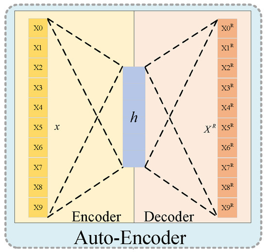
An auto-encoder [25] comprises two components: an encoder and a decoder, as illustrated in Figure 1. The encoder transforms n-dimensional input into m-dimensional latent variables where , forcing the neural network to learn the most informative features. The decoder reconstructs the latent variables h back to the original dimension. The optimal outcome is when the decoder’s output perfectly or approximately restores the original input, i.e., .
Figure 1.
Schematic diagram of auto-encoder structure.
Auto-encoders are unsupervised learning models. Based on backpropagation algorithms and optimization methods, they utilize the input data itself x as supervision to guide the neural network in learning a mapping relationship, thereby obtaining a reconstructed output . This process can be represented as:
where represents the encoder’s weight matrix, which is responsible for mapping input features to the hidden layer; denotes the encoder’s bias term, enhancing model flexibility; indicates the activation function; and are the decoder’s weights and bias, respectively; and is the decoder’s activation function.
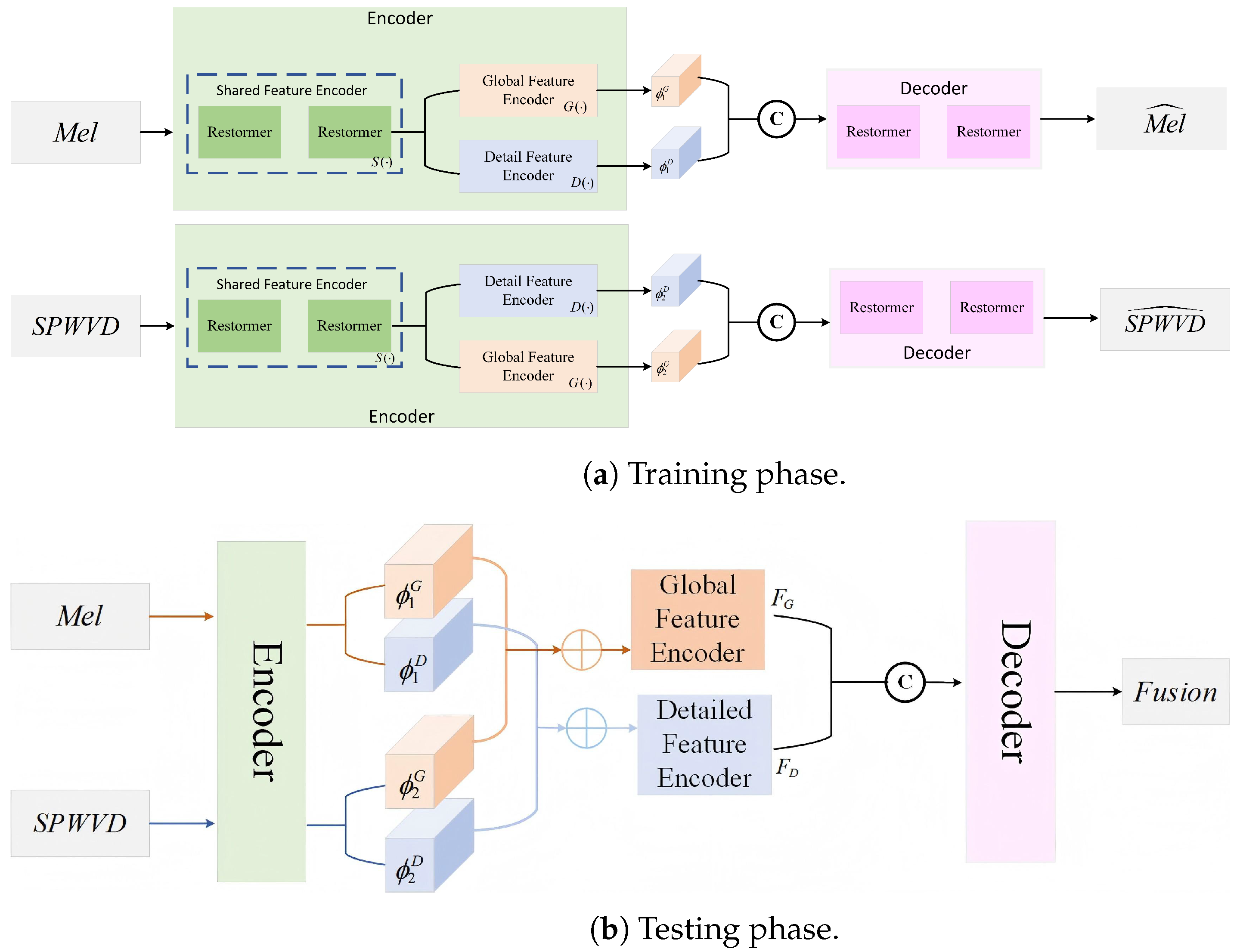
During the complete feature extraction and reconstruction stages, conventional supervised learning methods face significant limitations due to the lack of effective ground truth—that is, no known, true “ideal” feature fusion results serve as a standard. Therefore, the entire process is divided into training and testing phases, as illustrated in Figure 2, where Figure 2a depicts the training phase while Figure 2b shows the testing phase.
Figure 2.
Schematic diagram of the dual-branch auto-encoder network architecture.
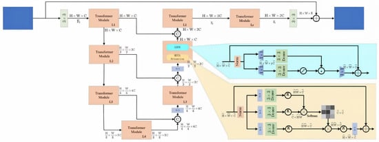
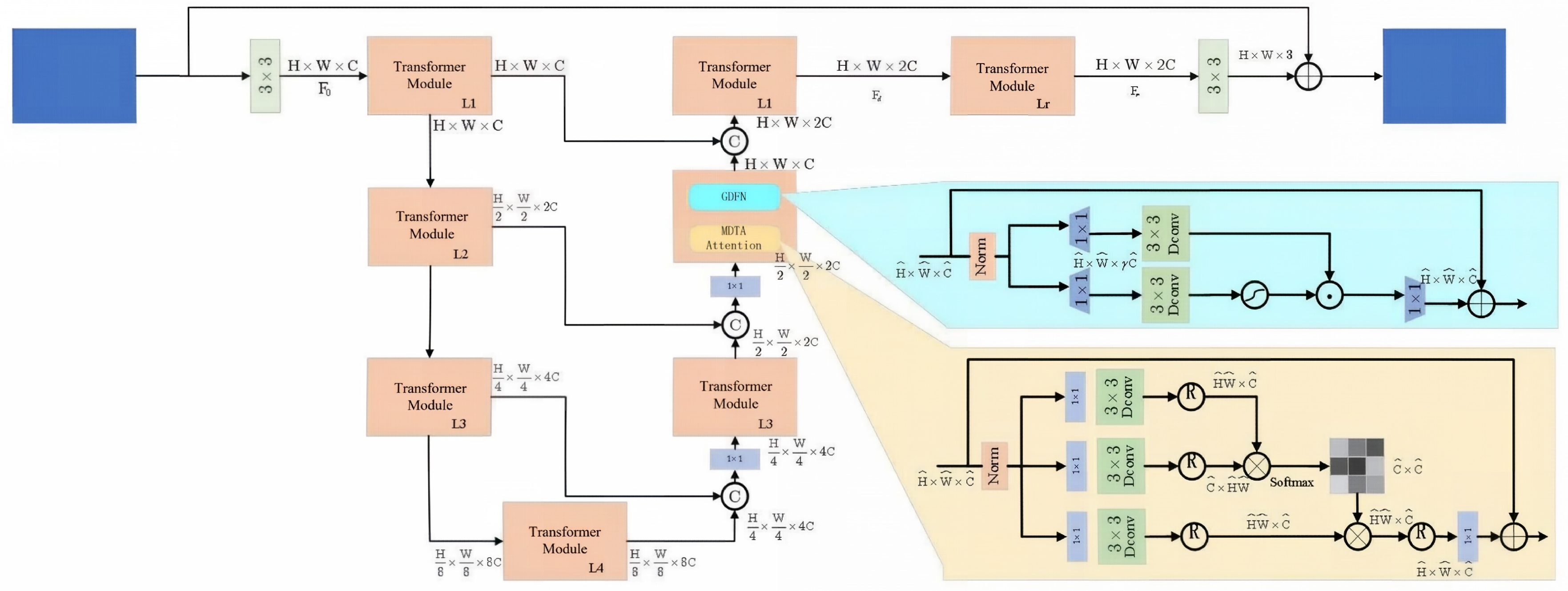
Before feeding the time–frequency feature image into the encoder, basic convolution operations are employed to extract feature information from the time–frequency feature image. This information is then passed to the encoder, where the dual-branch architecture is used to extract both global and detailed feature information. A shared feature encoder replaces the original basic convolution module, with its core being the Restormer. The Restormer combines the strengths of traditional convolutional neural networks and Transformers. Its self-attention mechanism captures relationships between long-range pixel within images, effectively extracting global features, while the convolutional layers extract local features. By integrating convolutional layers and self-attention, the Restormer model achieves a balance between detail and global features from the outset of feature extraction, preparing for subsequent refinement of both. Its network architecture is illustrated in Figure 3. The cores of Transformer module are: (a) multi-Dconv head transposed attention (MDTA) that performs (spatially enriched) query-key feature interaction across channels rather the spatial dimension, and (b) a Gated-Dconv feed-forward network (GDFN) that performs controlled feature transformation to allow useful information to propagate further [22].
Figure 3.
Diagram of Restormer model architecture.
During the training phase, a single time–frequency feature image is first used as input to fully train the auto-encoder. This enables it to accurately reconstruct the original time–frequency feature image, yielding an encoder capable of efficient feature extraction and a decoder with strong feature fusion and reconstruction performance for this specific data scenario. During the testing phase, different time–frequency feature images utilize the same trained auto-encoder network architecture to perform feature extraction and feature fusion across multiple time–frequency feature image datasets. The two types of time–frequency feature images are input into two encoder models sharing weights for feature extraction, respectively. Since the data is input in pairs, weight sharing enables the learning of similarities or differences between inputs. Ultimately, the feature-rich time–frequency feature fusion image dataset is used to accomplish underwater target recognition tasks.
Compared to directly utilizing extracted time–frequency features through methods like channel concatenation, the approach of performing feature extraction on time–frequency images using an auto-encoder network architecture and then performing feature fusion and reconstruction employs the encoder to extract low-dimensional features from the input images. This allows for the extraction of the most critical features within each type of image. Additionally, auto-encoders possess noise reduction capabilities, enabling the removal of noise and redundant information from the original input data during feature extraction [26], thereby enhancing the representation of target features.
2.1.2. Loss Functions
To better extract both detailed and global information while aligning with the scenario described in this paper, multiple loss functions have been designed within the total loss L, including the structural similarity loss , gradient loss , and perceptual loss . The equations are as follows:
- (1)
- Structural Similarity Loss
Structural Similarity Index (SSIM) [27] is an indicator for measuring the similarity between two images. It compares the similarity between the original input image I and the image after feature fusion and reconstruction, R, across three dimensions: luminance , contrast , and structure . The similarity between image I and image R is a function of these three components:
where the SSIM value closer to 1 indicates higher similarity between the result image after feature fusion and the original input time–frequency data image, preserving richer feature information.
The luminance component is defined as:
where and represent the average brightness of the input image and the reconstructed image after feature fusion, respectively.
The contrast component measures the intensity of brightness variation in an image, specifically the standard deviation of pixel values, defined as:
where and represent the variance of the input image and the reconstructed image after feature fusion, respectively.
For a given image data, both brightness and contrast can be quantified as single scalar values. However, the structural characteristics of an image cannot be fully represented by a single scalar and require description using a feature vector composed of all pixels. The influence of brightness and contrast factors must be eliminated to obtain accurate results during analyzing structure component. The structure component is defined as:
where indicates the covariance between I and R.
- (2)
- Gradient Loss
The gradient loss function calculates the edge information loss between the reconstructed image and the input image, as expressed by the following equations:
where is the gradient obtained by sharpening the image using the Laplacian operator. The Laplacian operator performs a mathematical convolution operation. Its definition and approximate discrete expression are as follows:
- (3)
- Perceptual Loss
Perceptual loss is typically computed by passing the input image and target image through a pre-trained neural network to obtain their feature representations within the network. These feature representations are then input into a loss function to calculate their Euclidean or Manhattan distance. The objective of perceptual loss is to minimize the distance between the input and target images in feature space, calculated as follows:
where denotes the feature representation extracted from the ith layer of the trained network model after inputting image I.
2.2. Balanced Ensemble Transfer Learning Method Based on Two-Stage Decoupled Fine-Tuning Learning Method
This section constructs a balanced ensemble transfer learning method based on a two-stage decoupled fine-tuning learning method. Transfer learning enables network models to adapt to the challenges of small-sample problems even under class imbalance conditions. The two-stage decoupled fine-tuning learning method divides the deep learning process into feature extraction and classification stages and performs decision-level fusion on multiple weak classifiers to obtain a strong classifier with optimal recognition capability through ensemble learning.
2.2.1. Two-Stage Decoupled Fine-Tuning Learning Method
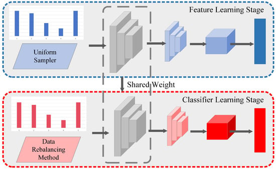
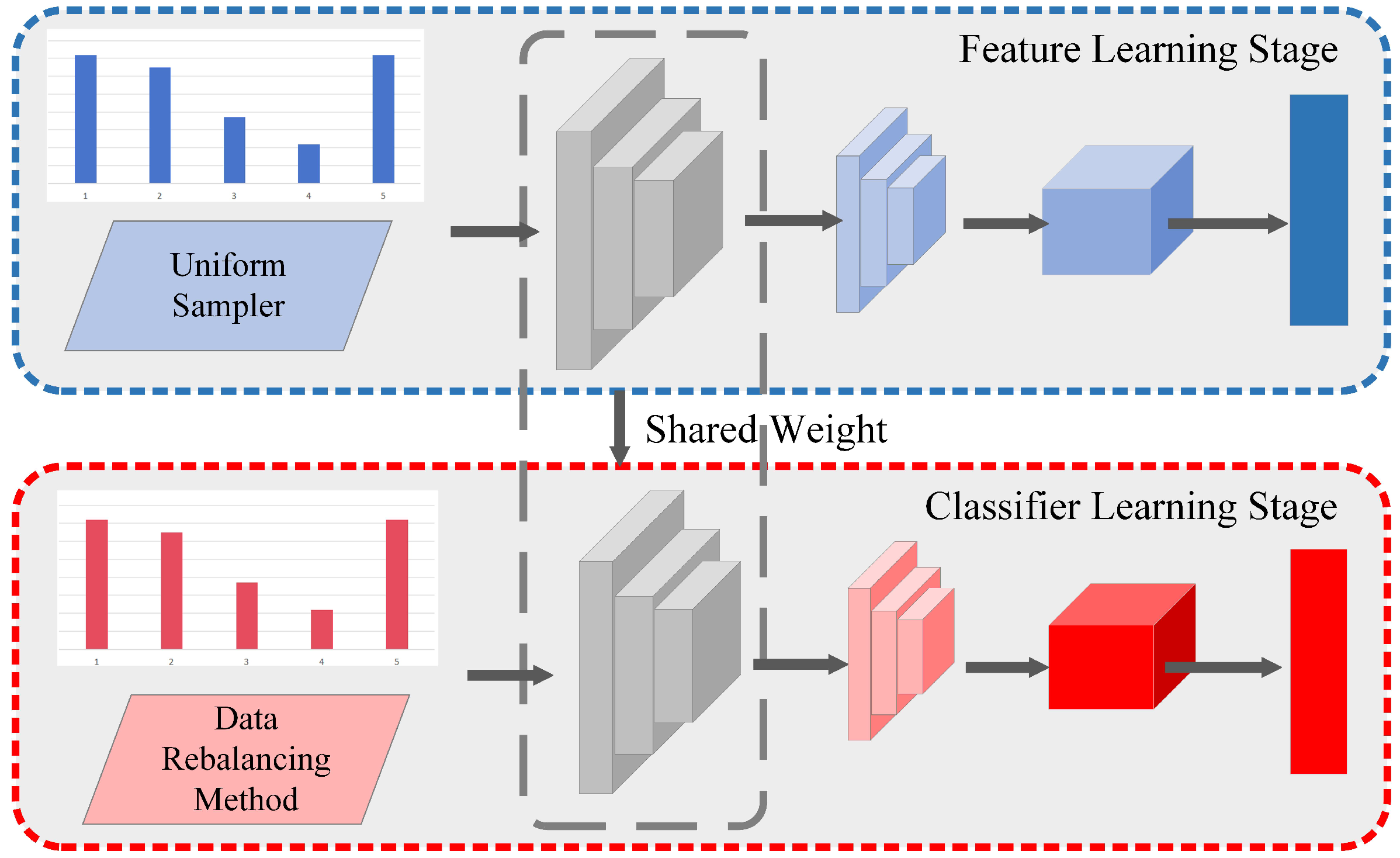
To achieve superior recognition classification performance while enhancing both the representational and classification capabilities of the network model, this paper employs a two-stage decoupled fine-tuning learning method, as illustrated in Figure 4. The traditional joint training approach (single-stage learning) is decomposed into two distinct learning stages: the feature learning stage and the classifier learning stage. Each stage employs specific methods for training or adjusting model weights [28]. First, during the feature learning stage, the model undergoes initial fine-tuning using a uniform sampler strategy on the class-imbalanced underwater target echo dataset, enhancing the model’s representational capacity based on the original data distribution. Second, during the classifier learning stage, a data-rebalancing method is applied for a second round of fine-tuning. The network weights used for training in this stage are derived from the fine-tuned weights obtained in the first stage. This constitutes the two-stage decoupled fine-tuning learning method.
Figure 4.
Diagram of the two-stage decoupled fine-tuning learning method.
2.2.2. Transfer Learning Method
Regardless of whether the sample distributions across underwater target classes are balanced, data scarcity remains a common challenge. This paper proposes pre-training the network using transfer learning (TL) method on top of fine-tuning the feature learning classifier. This approach further enhances the network model’s feature learning capabilities, mitigating the adverse effects of overall data scarcity on the model’s feature learning performance.
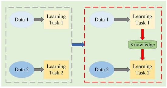
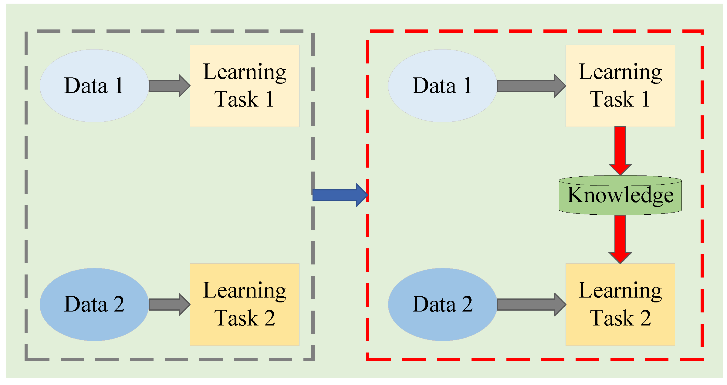
The traditional learning process and transfer learning schematic are shown in Figure 5, with the red box illustrating the transfer learning process. The characteristics of transfer learning align well with the need to mitigate the scarcity of samples in underwater target recognition and classification tasks. Therefore, this paper maps the ImageNet optical image dataset to the underwater target recognition task via transfer learning, achieving class feature matching and mapping for underwater targets.
Figure 5.
Schematic diagram of transfer learning.
2.2.3. Multiple Balanced Sampling Optimization Method
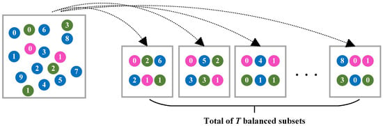
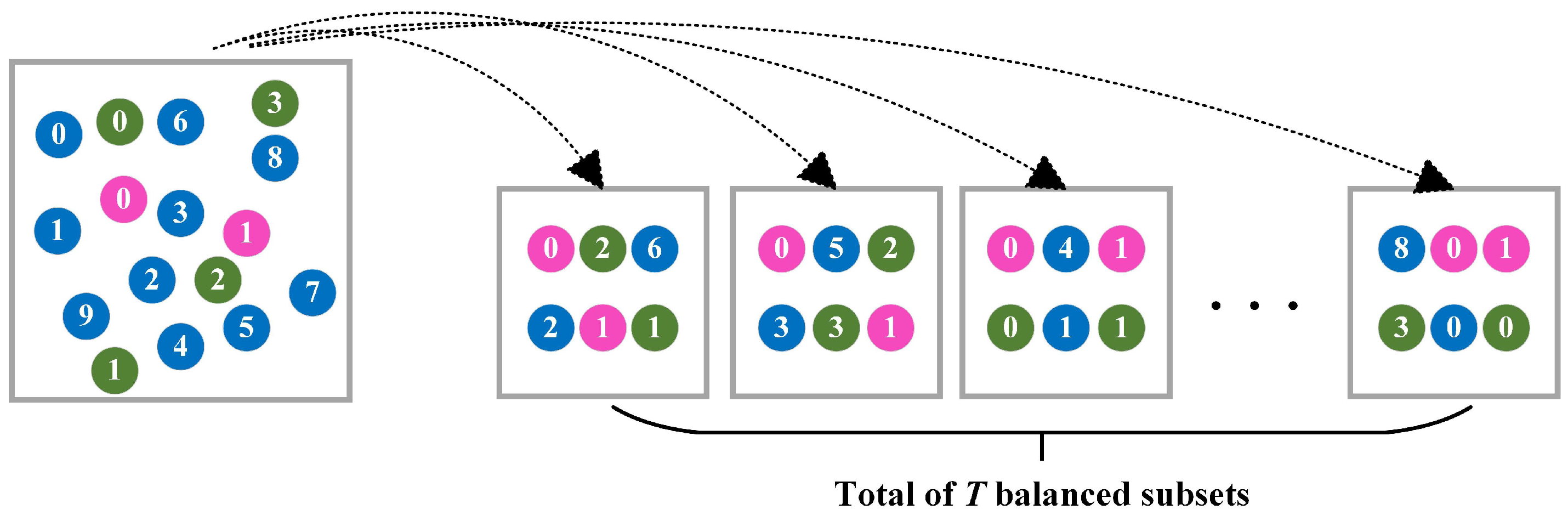
To maximize data utilization while avoiding overfitting and underfitting, this paper employs a multiple-balanced-sampling optimization method. At the data level, it performs dataset balancing for class-imbalanced underwater targets. The schematic of this method is shown in Figure 6. Compared to traditional resampling methods, this approach significantly improves classification performance for minority class samples while enhancing overall classification accuracy.
Figure 6.
Schematic diagram of multi-balance sampling method.
During multi-balanced sampling, N classes of underwater targets are assumed and denoted as . The training samples corresponding to these classes are organized into N lists. A class is randomly selected from , and one sample is then randomly drawn from the corresponding training sample list . This procedure is repeated to construct multiple balanced mini-batch subsets, yielding a total of T balanced subsets.
2.2.4. Classifier Selection and Ensemble Learning Methods
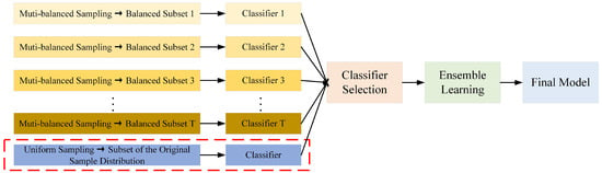
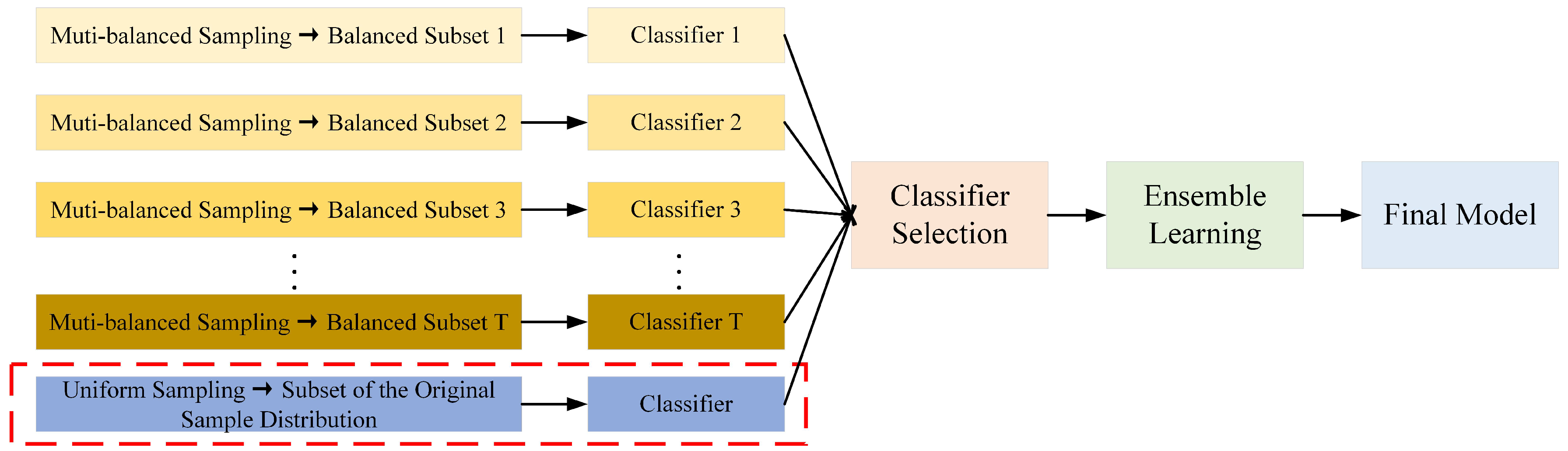
After the two-stage decoupled fine-tuning task, a total of trained classifiers were obtained. This includes one classifier fine-tuned by the feature learner in the first stage, plus T classifiers trained using the first-stage fine-tuned network model through T rounds of multiple balanced sampling. By integrating multiple classifiers, the random error and bias of a single model can be reduced, enhancing the model’s robustness to data and achieving better recognition performance. The process, illustrated in Figure 7, comprises two parts: classifier selection and ensemble learning, ultimately yielding a classifier model with superior recognition and classification performance.
Figure 7.
Schematic diagram of ensemble learning process.
- (1)
- Classifier Selection Method
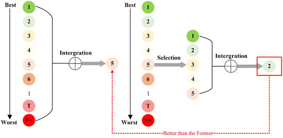
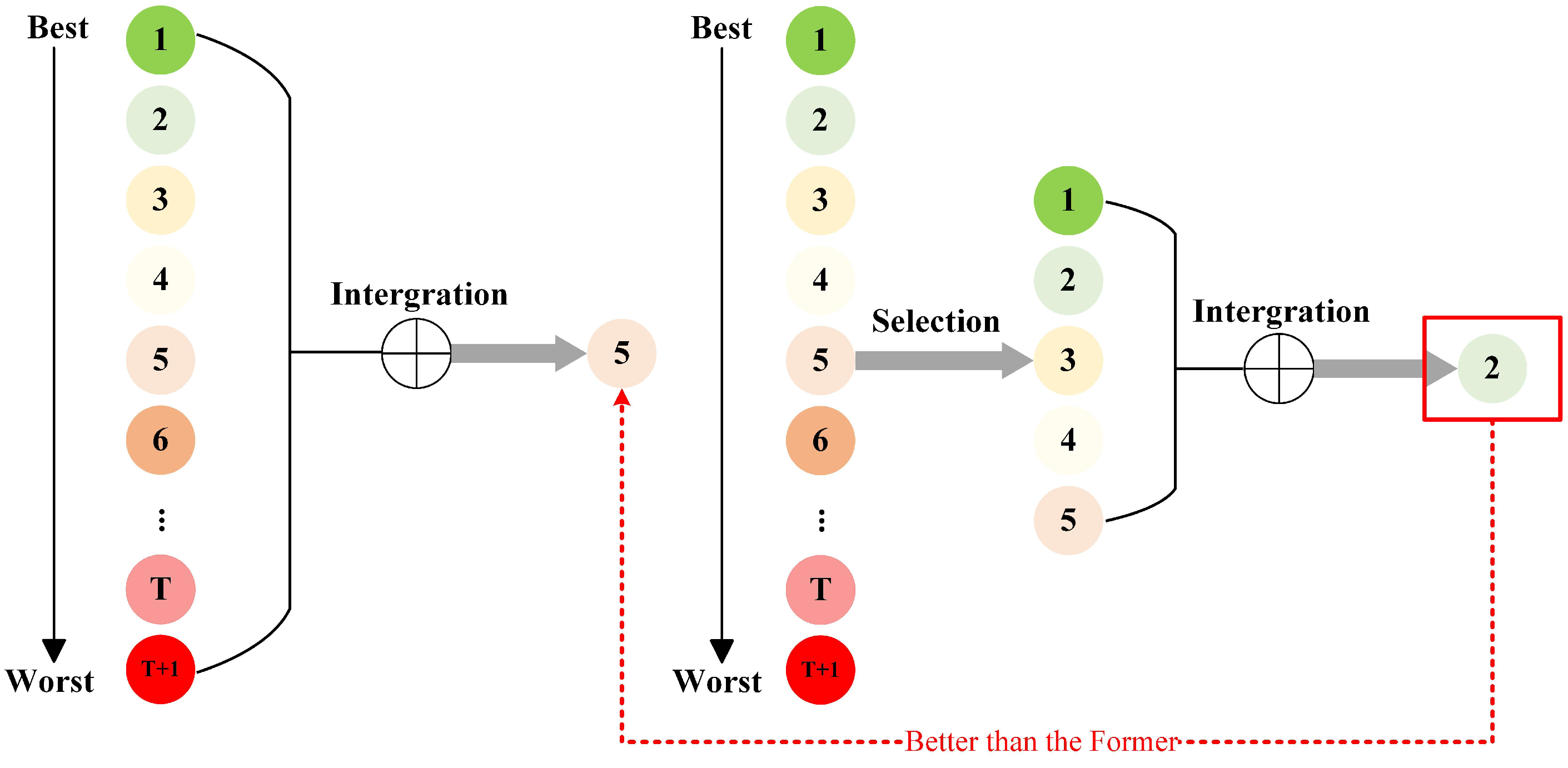
As described above, training yields base classifiers. Integrating a subset rather than all classifiers yields superior performance. Therefore, this paper employs a classifier selection method: ranking and filtering base classifiers using relevant indicators to retain a subset of higher-performing classifiers for subsequent ensemble learning. The selection principle is illustrated in Figure 8.
Figure 8.
Schematic diagram of the basic classifier selection principle.
Simultaneously, the parameter is introduced as the classifier retention coefficient. Its specific value is defined as , retaining the classifier with the average ranking between the two sorted lists. The number of base classifiers retained is defined by the following equation:
where denotes floor division.
After multiple experiments, is set to 0.6 in this paper.
- (2)
- Classifier Ensemble Learning Method
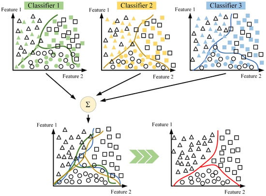
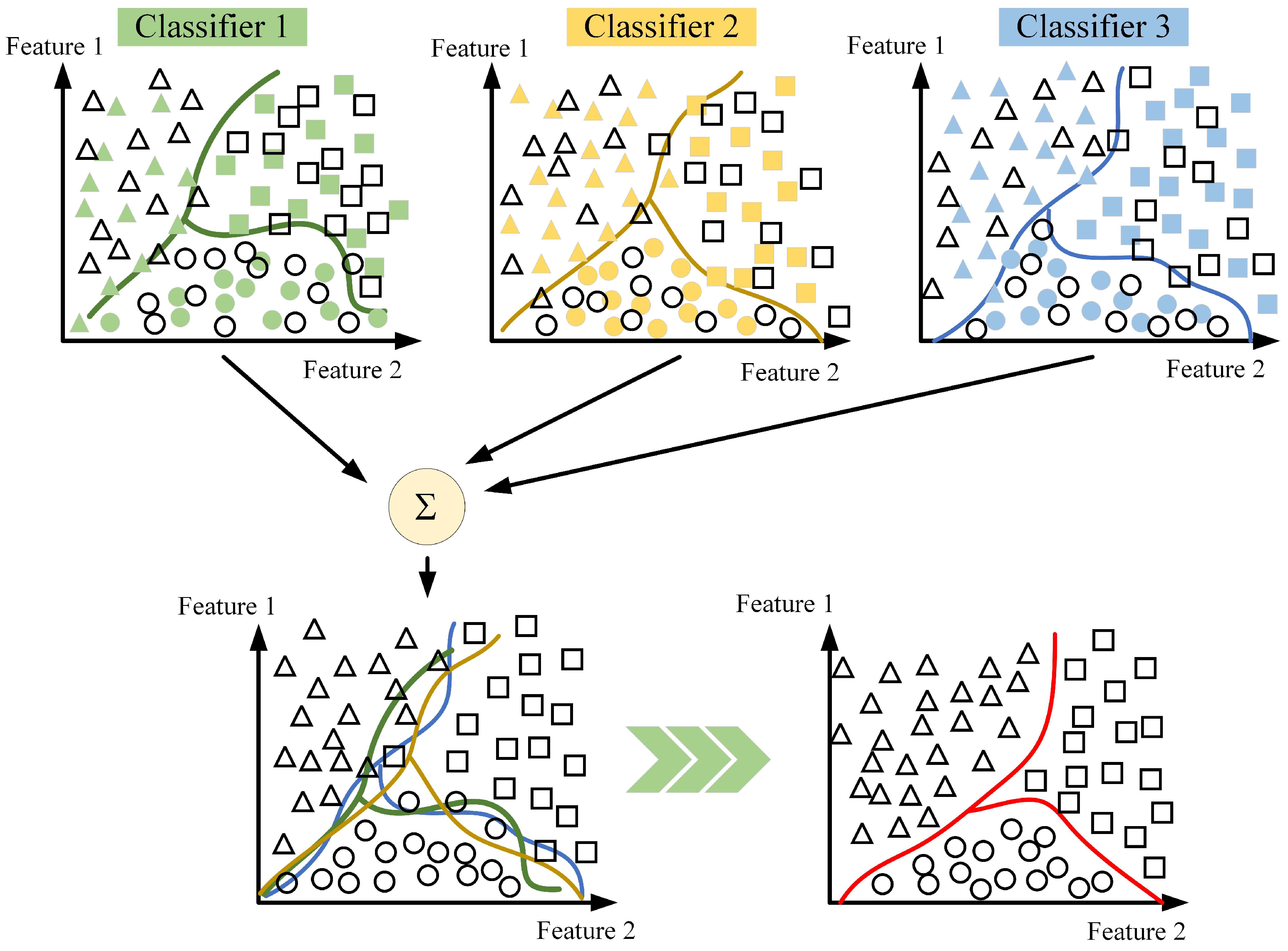
Ensemble learning is a powerful machine learning approach in the field of artificial intelligence. It integrates multiple classifiers trained on different features, ultimately yielding clearer class boundaries and a more effective classifier model [29]. The specific process is illustrated in Figure 9.
Figure 9.
Schematic diagram of ensemble learning method.
This paper employs a weight-averaging method to average the parameters of multiple classifiers, thereby generating new classifier models. Assuming there are N classes of underwater targets, represented as . denotes the weight assigned to the classifiers during selection, where and indicates retaining the classifier, while signifies removing it. When a test sample is input into the classifiers, its predicted label is . The one-hot encoding of the output label is , and indicates that the classifier predicts the test sample as belonging to the class .The predicted Boolean value is represented as , where a higher indicates a greater likelihood of classifying the sample as the target . The parameters of the classifiers are defined as . Ultimately, the prediction label results of the classifier ensemble network model retained after screening are defined as . The average of the parameters of the retained classifiers is denoted as . Then, the parameters of the classifiers after ensemble learning, expressed through weight averaging, are represented as:
where the output label is obtained by feeding the test sample into the ensemble learning classifier.
2.3. Underwater Target Recognition Method Based on Feature Fusion and Balanced Ensemble Transfer Learning
Based on the aforementioned methods, this paper proposes an underwater target recognition method based on feature fusion and balanced ensemble transfer learning.
First, time–frequency image feature fusion is performed using a LiT-INN dual-branch auto-encoder network architecture. By enriching the feature information within images, the discrimination between feature images is enhanced, thereby improving recognition accuracy. Different time–frequency transformation methods map echo information to distinct time–frequency feature spaces. A basic dual-branch auto-encoder network was employed to perform feature fusion and reconstruction of time–frequency images, with its loss function optimized. The dual-branch encoder in the auto-encoder was optimized using Lite-Transformer (LiT) and Invertible Neural Networks (INN), establishing a LiT-INN dual-branch auto-encoder architecture that further enhances feature extraction quality while minimizing information loss.
Second, balanced ensemble transfer learning is constructed based on a two-stage decoupled fine-tuning learning method. Transfer learning pre-trained the network to maintain adaptability to small-sample problems under class imbalance. To simultaneously preserve representational and classification capabilities, a two-stage decoupled fine-tuning learning method was employed. Using a class-imbalanced underwater feature fusion dataset, the feature extractor and classifier were fine-tuned using the uniform sampler strategy and a multiple balanced sampling optimization method, respectively. Through ensemble learning, multiple weak classifiers are integrated into a strong classifier, further addressing the degradation of deep learning model recognition capabilities under class imbalance. This enhances recognition accuracy for classes with fewer samples and improves overall recognition performance.
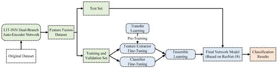
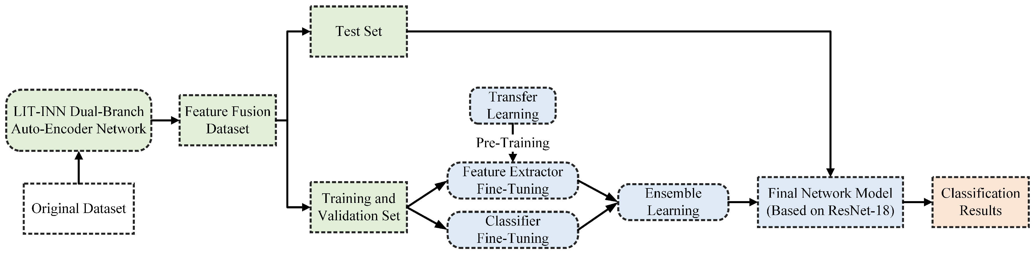
The proposed underwater target recognition method based on feature fusion and balanced ensemble transfer learning is illustrated in Figure 10.
Figure 10.
Schematic diagram of the underwater target recognition method based on feature fusion and balanced ensemble transfer learning.
3. Experiment
This section comprises three parts: the first part presents evaluation indicators, the second part describes simulation experiments, and the last part details field tests. These collectively validate the effectiveness of the proposed underwater target recognition method based on feature fusion and balanced ensemble transfer learning.
3.1. Evaluation Metrics
Considering the issue of imbalanced distribution in the number of samples across different target classes, the primary focus is on the accuracy of classes with fewer samples. Therefore, to accurately assess the effectiveness of the proposed method for addressing the imbalanced distribution of underwater target samples, the following four metrics were added to the result analysis: score, Precision–Recall Curve, Area Under the Curve (AUCPR, AP), and score.
For binary classification tasks, the score is defined as follows:
True Positive Rate () and Recall rate R in the PR curve are given by:
True Negative Rate () is defined as:
Precision P in the PR curve is defined as:
where , , , and represent the four scenarios: predicted and actual values are both positive; predicted negative but actual positive; predicted positive but actual negative; and both predicted and actual values are negative.
The score is defined as:
In multi-class classification tasks, any two classes form a binary confusion matrix. In this case, calculate the precision and recall rate for each confusion matrix, then average them to obtain and , and compute the score. For a three-class classification problem, the specific calculation equation is expressed as follows:
3.2. Simulation Experiment
3.2.1. Simulated Time–Frequency Image Dataset Construction
This paper primarily employed the acoustics module within the COMSOL Multiphysics 6.0, combined with partial differential equation solvers, to mathematically model the acoustic scattering characteristics of the target model. By calculating the inverse morphological function of the target and applying frequency-domain indirect computation methods, the time-domain echo signals of the simulated target were ultimately obtained.
Schematic diagrams of the three simulated underwater targets are shown in Figure 11. All three are volumetric targets. Target 1 is modeled as a ship bottom with a single-screw propeller; Target 2 as a ship bottom with a twin-screw propellers; and Target 3 as an unmanned underwater vehicle (UUV).
Figure 11.
Schematic diagram of three simulated target classes.
When constructing target echo models, a Linear Frequency Modulation (LFM) signal was employed as the transmitted signal. The target’s characteristics, such as the target’s intensity and scale, were simulated using parameters such as the brightness fluctuation and time delay of the echo signal.
The reflective characteristics of underwater targets can be characterized by the target strength parameter. By linearly superimposing the amplitudes of specular reflections and angular reflections, the target strength parameter of the underwater target can be obtained. To more closely approximate real underwater conditions, noise and reverberation components were introduced into the simulated underwater target echo signals. The signal-to-noise ratio (SNR) was set to −25 dB, while the signal-to-reverberation ratio (SRR) was set to −10 dB.
Given that the simulated target echo dataset originates from the reflection of LFM signals by three underwater targets across multiple cycles, this dataset encompasses echo information from these targets at 361 distinct angles. To more accurately simulate potential class imbalance in underwater target recognition tasks, the following sampling strategy was applied within a single cycle: For Target 1, 80 angles were randomly selected, forming an array of dimensions (80, 60,000); For Target 2, 323 angles were randomly sampled, yielding an array of dimensions (323, 60,000). For Target 3, 90 angles were randomly selected, forming an array of dimensions (90, 60,000). Through clipping operations, only segments containing target echo signals were retained, and labeling was performed on the initial column of the dataset. The imbalance ratio () of the dataset is defined as follows:
where denotes the number of samples in the most abundant class among underwater targets, and denotes the number of samples in the least abundant class.
Figure 12 displays the visualization results of the echo signal at a specific incident angle. The time-domain image is plotted with the time axis as the horizontal coordinate and the echo amplitude as the vertical coordinate.
Figure 12.
Three-Class Target time-domain waveforms.
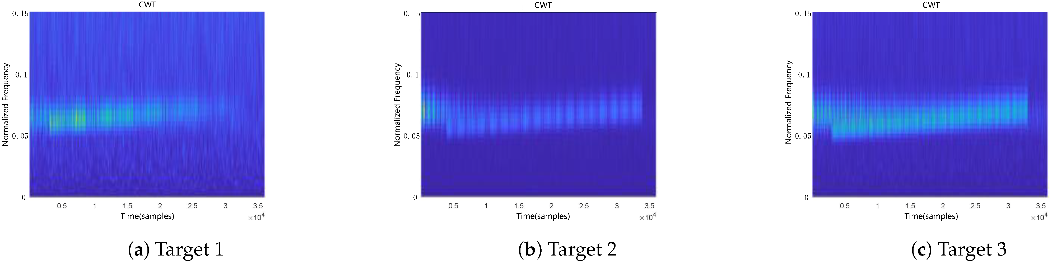
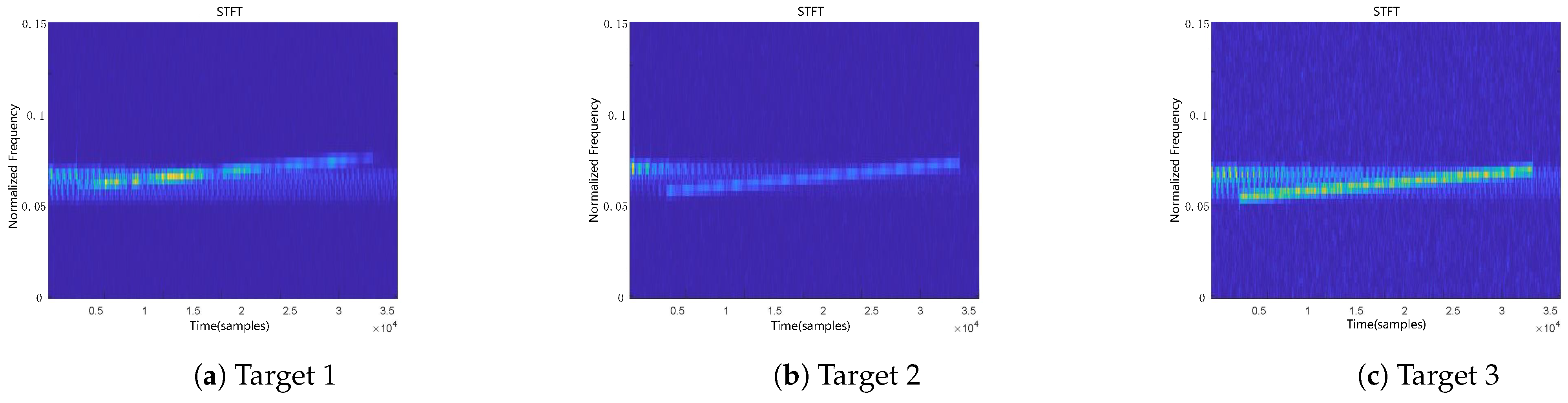
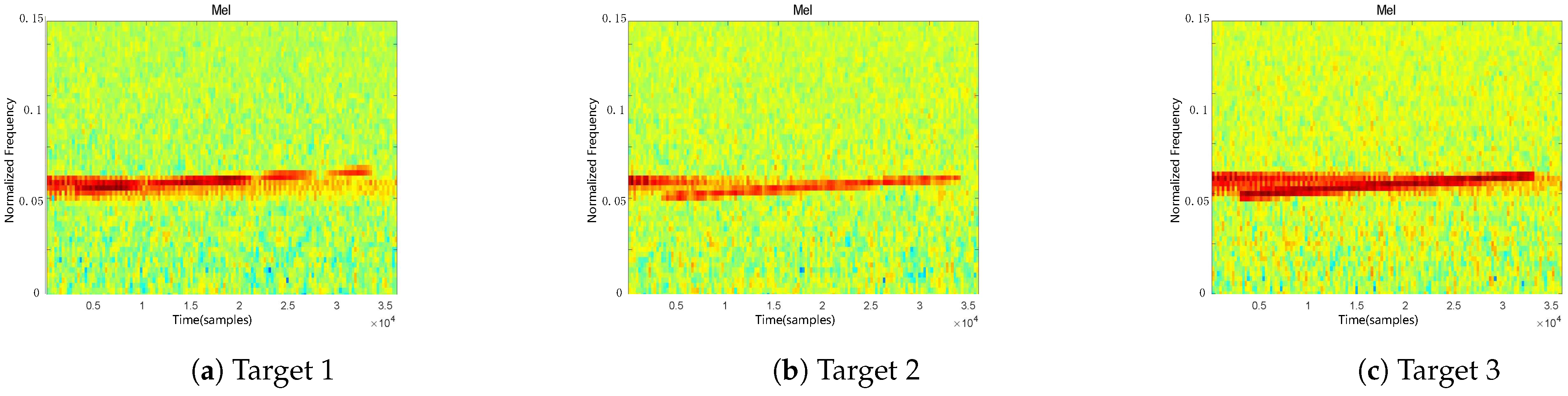
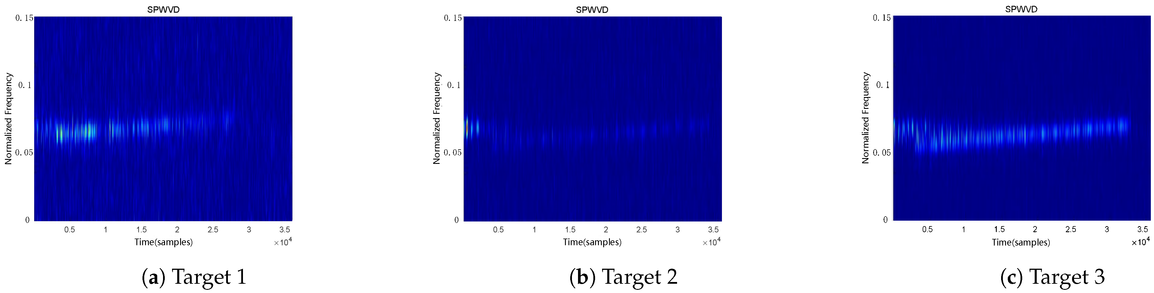
Four time–frequency datasets were constructed using Continuous Wavelet Transform (CWTs) [30], Short-Time Fourier Transform (STFT) [31], Mel-Spectrogram Analysis (Mel) [32], and Smooth Pseudo Wigner–Ville Distribution (SPWVD) [33], shown in Figure 13, Figure 14, Figure 15 and Figure 16. The sampling frequency was set to 100 kHz. Table 1 displays the specific dataset composition.
Figure 13.
CWT images of three target classes.
Figure 14.
STFT images of three target classes.
Figure 15.
Mel spectrogram images of three target classes.
Figure 16.
SPWVD images of three target classes.
Table 1.
Composition of multi-spectral time–frequency image datasets.
After multiple simulation experiments, the balanced subset size T was set according to the dataset imbalance ratio , which is defined as shown in Equation (20), and the balanced subset size T is selected based on the following equation:
where denotes floor rounding.
Since the total number of samples in the majority class is , and samples are drawn in each round, the maximum number of rounds of sampling without replacement is . When is not an integer multiple of , the number of samples remaining after the final round is less than , making it impossible to form a complete balanced subset. Therefore, a maximum of balanced subsets can be constructed, ensuring both the full utilization of information from the majority class and diversity among subsets due to sampling variations.
To ensure adequate learning for the class with the fewest samples, the total number of samples in each balanced subset was set based on its specific count. Additionally, the total number of uniformly sampled samples used during the feature extractor fine-tuning phase was kept consistent with the sample count in that balanced subset. Based on the dataset constructed with underwater targets in this paper, the total sample size for the balanced subset was set to 240, with 80 samples for each of the three target classes. The composition of the balanced subset data is shown in Table 2. Based on the above content, four balanced subsets were obtained through multiple balanced sampling methods, i.e., .
Table 2.
Composition of each dataset.
To enhance the accuracy of conclusions, a five-fold cross-validation method was employed. This involved randomly dividing each target data class in the dataset into five subsets. Each subset was used as a test set once, while the remaining four subsets served as training and validation sets. The specific division is shown in Table 3.
Table 3.
Echo dataset after five-fold cross-validation.
3.2.2. Ablation Study
The value of the classifier screening coefficient determines the number of weak classifiers retained after screening. Multiple weak classifiers are obtained by training on multiple different balanced subsets, with each weak classifier utilizing distinct data. Ensemble learning can fuse the best-performing weak classifiers at the decision level. To verify that integrating a subset rather than all weak classifiers yields superior results, an ablation study was conducted. This involved varying only the value of to observe its impact on final recognition performance. Given a dataset with an imbalance ratio () of 4.04, a total of five weak classifiers were obtained. The ensemble results under different filtering coefficients were evaluated using and scores, as shown in Table 4.
Table 4.
The effect of varying on recognition results.
As shown in Table 4, the best results are achieved when the screening coefficient is set to 0.6, with both and scores reaching 0.941—exceeding results under other values. This validates that conditionally filtering weak classifiers for ensemble learning, rather than incorporating all weak classifiers, yields the optimal ensemble classifier. Based on these findings, the screening coefficient is set to 0.6 for the fusion feature dataset with an imbalance ratio = 4.04 used in this paper.
3.2.3. Comparative Experimental Validation
This paper employed the ResNet [34] series network architecture, utilizing time–frequency feature image datasets to accomplish underwater target recognition tasks. The simulation environment consisted of a desktop workstation with two Intel Xeon Platinum 8373C CPU, two Nvidia RTX 3090 GPU, and 512 GB of memory. The operating system was CentOS 7, with PyCharm 2021.2.2 serving as the software compiler. The framework was PyTorch 2.0.1, and the CUDA version was 11.8. As shown in Table 5, ResNet-18 achieves the highest recognition accuracy across all experiments. Furthermore, it demonstrates optimal performance when applied to both the Mel-spectrogram dataset and the SPWVD image dataset. Consequently, the Mel-spectrogram and SPWVD image datasets were selected as the primary datasets for subsequent research, with ResNet-18 serving as the foundational network architecture.
Table 5.
Test set recognition accuracy of ResNet series networks on the simulation dataset.
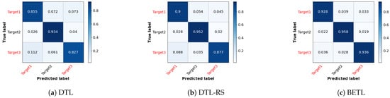
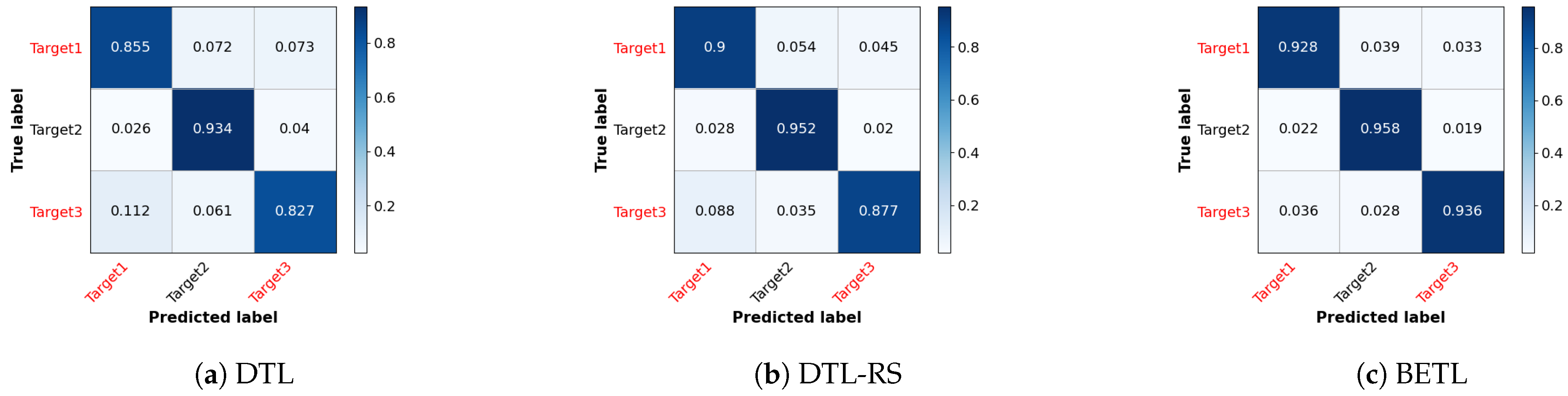
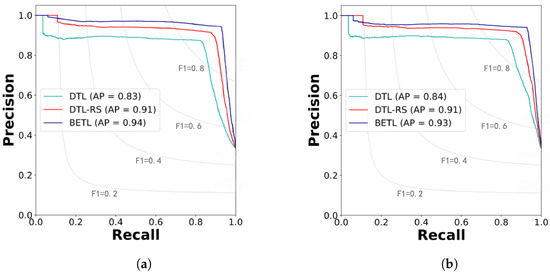
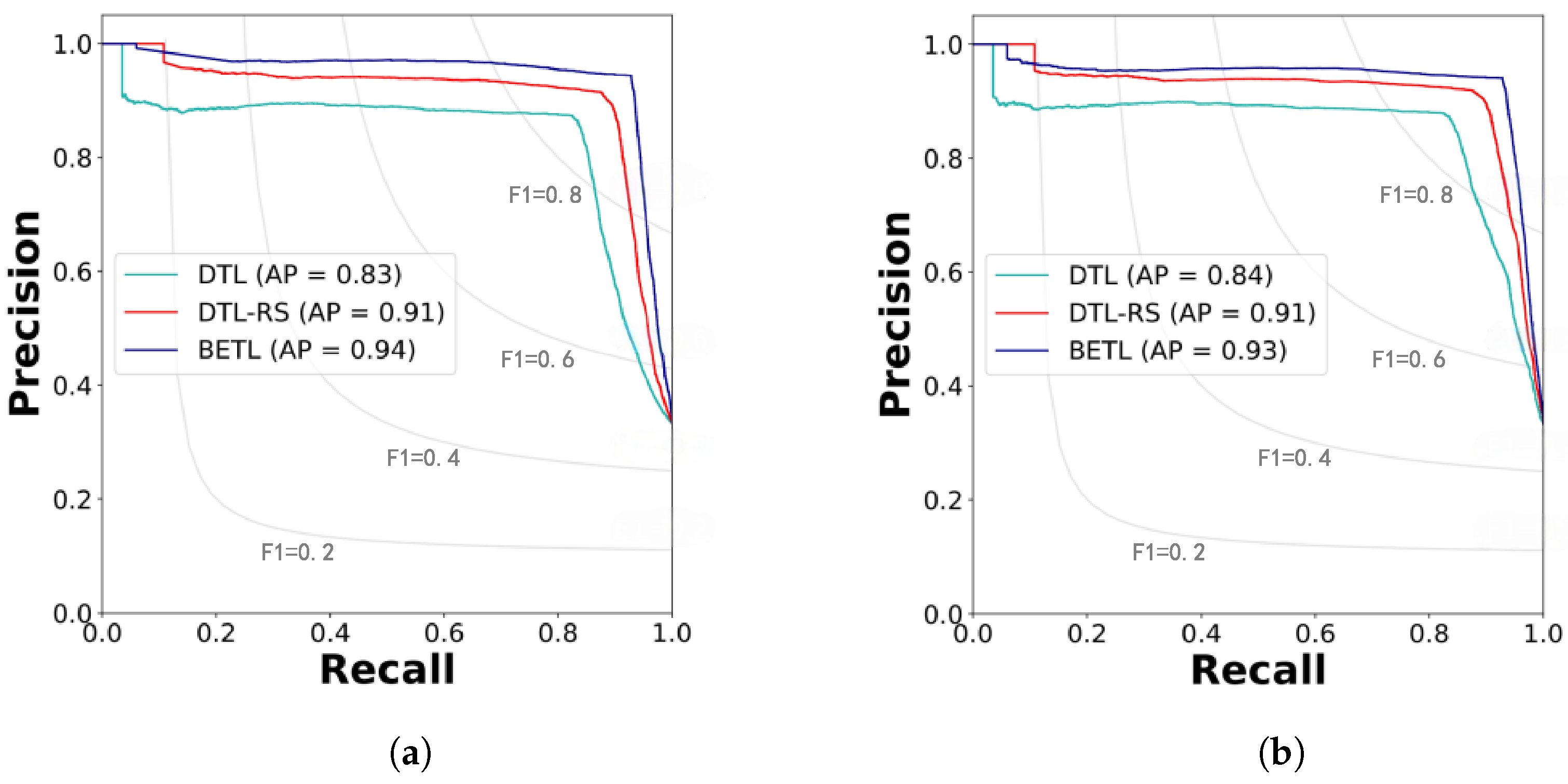
The network training settings were as follows. Considering that the learning rate needs to be adjusted based on the backbone network during transfer learning, for the ResNet-18 architecture used in this paper, the learning rates for the encoders and classifiers were set to 0.01 and 0.1, respectively. During the balanced ensemble transfer learning phase, the learning rate was set to 0.01, the weight decay was set to 0.001, the batch size was 16, and the training cycle was set to 5. A unified regularization process was applied before inputting data into the network, yielding mean values of [0.485, 0.456, 0.406] and standard deviations of [0.229, 0.224, 0.225]. The cross-entropy (CE) loss function was ultimately employed during the training phase. During the training phase of balanced ensemble learning, the balanced subsets comprised 240 samples, with 80 samples per target class. The number of balanced classifiers T was set to an integer close to the dataset imbalance ratio, i.e., , resulting in a total of five weak classifiers. The ensemble classifier selection coefficient was set to . Specific results are shown in Figure 17 and Figure 18 and Table 6.
Figure 17.
Confusion matrix results.
Figure 18.
Results. (a) Results for target class with the smallest sample number; (b) overall results for all target classes.
Table 6.
Results of different methods based on the simulation dataset.
As shown in Figure 17, the recognition accuracy of target 2 with the largest number of samples increases from 93.4% to 95.8%. The recognition accuracy of targets 1 and 3 with fewer samples rises from 85.5% and 82.7% to 92.8% and 93.6%, respectively, representing significant improvements for both.
Figure 18 demonstrates that both overall recognition performance and recognition performance for classes with fewer samples have improved. For the class with the fewest samples, the average recognition accuracy increases from 0.83 to 0.94, and the overall average recognition accuracy improves from 0.84 to 0.93. A value closer to 1 indicates a superior recognition performance. Before employing the proposed method, underwater target recognition was constrained by targets 1 and 3, which failed to provide sufficient quantity and quality of feature information. This prevented the neural network from learning effective information, resulting in weak overall performance.
As shown in Table 6, the score is 0.869 through deep transfer learning. By incorporating resampling methods, this score improves to 0.910. Finally, the method proposed in this paper achieved a score of 0.941. The scores obtained from the three methods are 0.871, 0.909, and 0.941, respectively.
These validate the effectiveness of the proposed underwater target recognition method based on feature fusion and balanced ensemble transfer learning.
3.3. Field Testing
3.3.1. Field Test Dataset Construction
To validate the effectiveness and generalization of the proposed method in actual scenarios, field test data was collected and analyzed. The collected field test datasets encompassed three distinct classes of underwater targets. Data acquisition employed a uniform linear array comprising 24 elements. To extract meaningful information from raw 24-element array echo data, a series of preprocessing steps must be performed. These include filtering, reverberation reduction, beamforming, and data clipping, ultimately generating beam domain echo data suitable for analysis. Target 1 has 363 sets of echo data, Target 2 has 323 sets of echo data, and Target 3 has 312 sets of echo data. The specific composition of the echo datasets is shown in Table 7.
Table 7.
Distribution of sample sizes by target class.
Based on the acquired underwater target echo data, two echo datasets with different imbalance ratios were constructed. In addition to the imbalance ratio = 4.04 set for the simulation data mentioned earlier, an additional dataset with an imbalance ratio = 5.38 was created. Randomly selecting 80% of the data as the training and validation sets, and 20% as the test set, the data composition of the underwater target echo datasets under each imbalance rate is shown in Table 8 and Table 9 below.
Table 8.
Distribution of sample sizes by target class (IR = 4.04).
Table 9.
Distribution of sample sizes by target class (IR = 5.38).
3.3.2. Target-Discriminative Validation
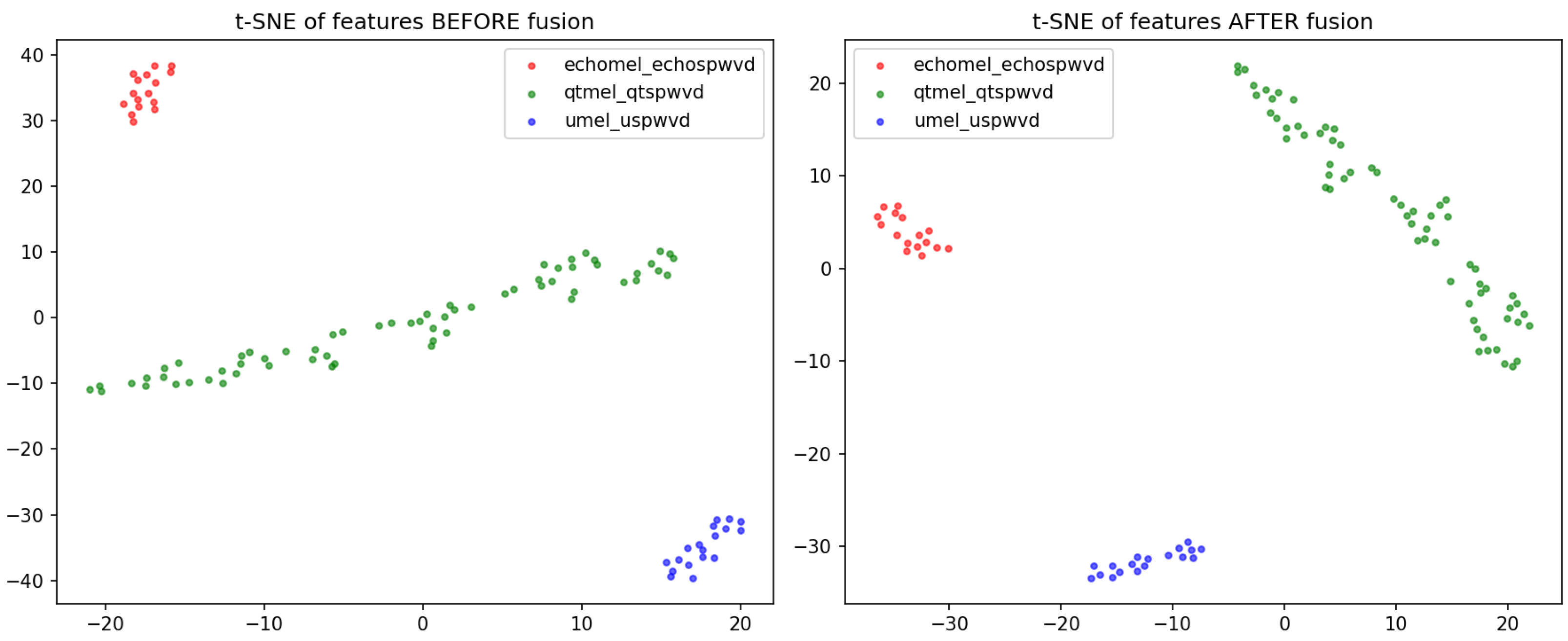
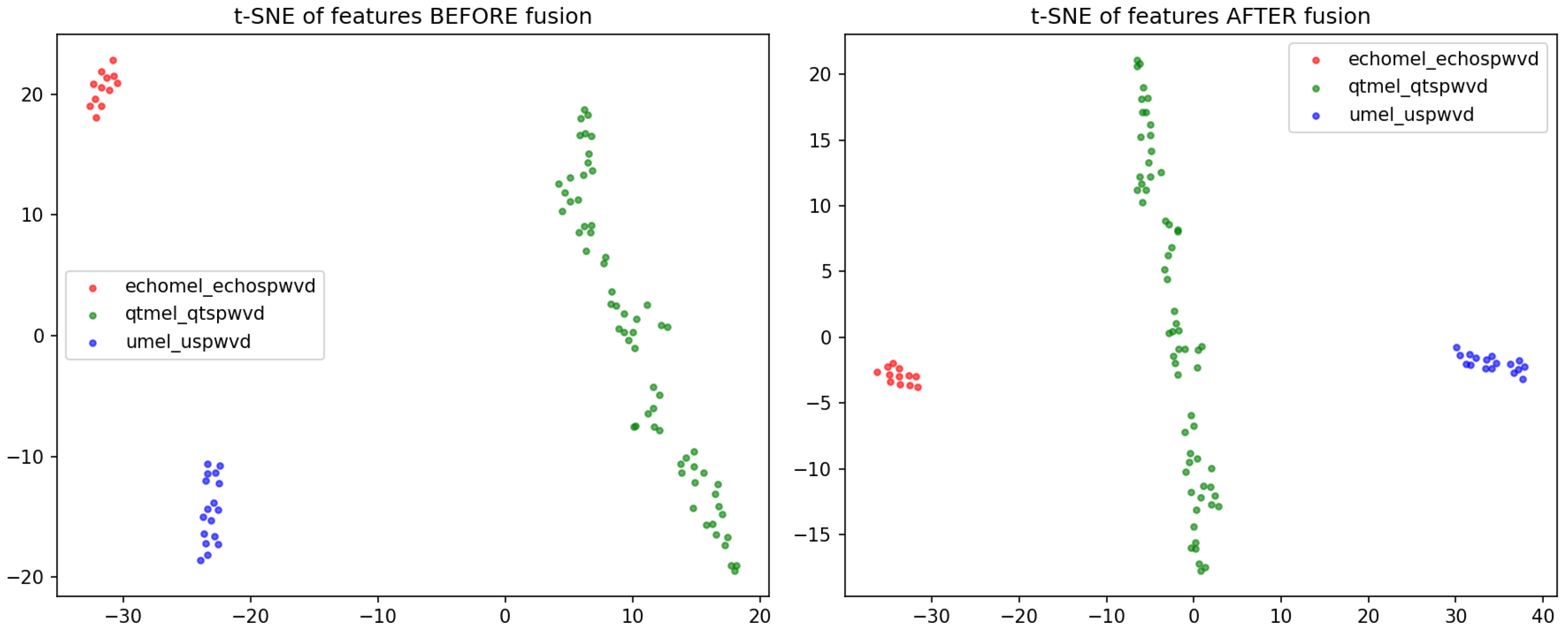
In order to prove that the learned fused features genuinely capture optimal target-discriminative information, feature spaces were visualized before and after feature fusion using t-SNE plots, and two widely used metrics for assessing feature separability were employed. The first is the Calinski–Harabasz (CH) score, which is based on the ratio of inter-class dispersion to intra-class dispersion; a higher value indicates a better clustering performance. The Davies–Bouldin (DB) index measures the ratio of the average distance between samples within a class to the distance from the class center; a smaller value indicates greater compactness within classes and better separation between classes. Feature space visualization is shown in Figure 19 and Figure 20 and quantitative separability metrics are shown in Table 10 and Table 11.
Figure 19.
t-SNE plots before and after feature fusion (IR = 4.04).
Figure 20.
t-SNE plots before and after feature fusion (IR = 5.38).
Table 10.
Quantitative separability metrics (IR = 4.04).
Table 11.
Quantitative separability metrics (IR = 5.38).
As shown in Table 10 and Table 11, when the dataset imbalance ratio was 4.04, the fused features achieved a 97.1% improvement in the Calinski–Harabasz score and a 35.1% reduction in the Davies–Bouldin index, indicating that the proposed fusion method significantly enhances the inter-class separability and intra-class compactness of the features, thereby effectively improving the discriminative power between different targets. As the imbalance ratio increases to 5.38, the fused features still achieve positive results, with a 56.5% improvement in the CH score and a 21.5% reduction in the DB index, demonstrating that the method remains effective on even more imbalanced datasets.
3.3.3. Experimental Validation
- (1)
- = 4.04
Five-fold cross-validation was employed to enhance the accuracy of conclusions. The training settings and balanced ensemble learning training phase maintained consistent balanced subset partitioning with simulation experiments. The number of balanced classifiers was set to an integer close to the dataset imbalance factor, i.e., . The ensemble classifier selection coefficient was set to 0.6. Specific results are shown in Figure 21 and Figure 22 and Table 12 below.
Figure 21.
Confusion matrix results.
Figure 22.
Results. (a) Results for the target class with the smallest sample number; (b) overall results for all target classes.
Table 12.
Results of different methods based on a field test dataset.
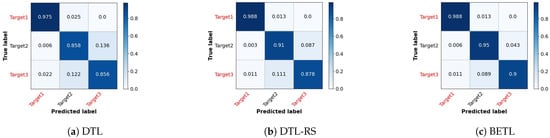
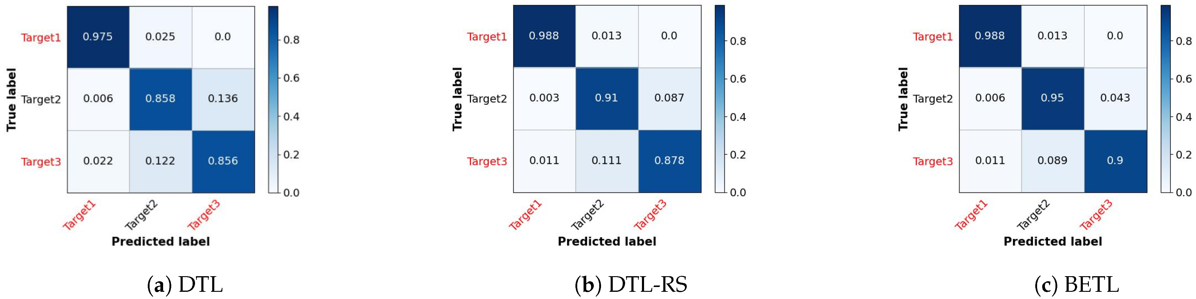
Among the three underwater target classes, Target 1 exhibits high discrimination due to its inherent feature information, remaining easily distinguishable even with a small sample size. Targets 2 and 3 show poor discrimination and are prone to confusion.
As shown in Figure 21, by incorporating data resampling strategies, the recognition accuracy for the three target classes improves from 97.5%, 85.8%, and 85.6% to 98.8%, 91.0%, and 87.8%, respectively. Target 1 is clearly distinguishable, while Target 2 and Target 3 exhibit partial confusion. Nevertheless, the overall results still outperform the recognition accuracy through deep transfer learning methods based on fusion results. The recognition accuracy for Target 2 improves by approximately 5.2%, and that for Target 3 improves by approximately 2.2%. Using the proposed method, the recognition accuracy for the three underwater target classes reaches 98.8%, 95.0%, and 90.0%, respectively, with significant improvements observed for both Target 2 and Target 3.
As shown in Table 12, the score through deep transfer learning is 0.894; it improves to 0.924 by incorporating resampling methods, and ultimately reaches 0.945 using the proposed method. The scores based on the three methods are 0.893, 0.924, and 0.946, respectively.
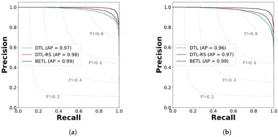
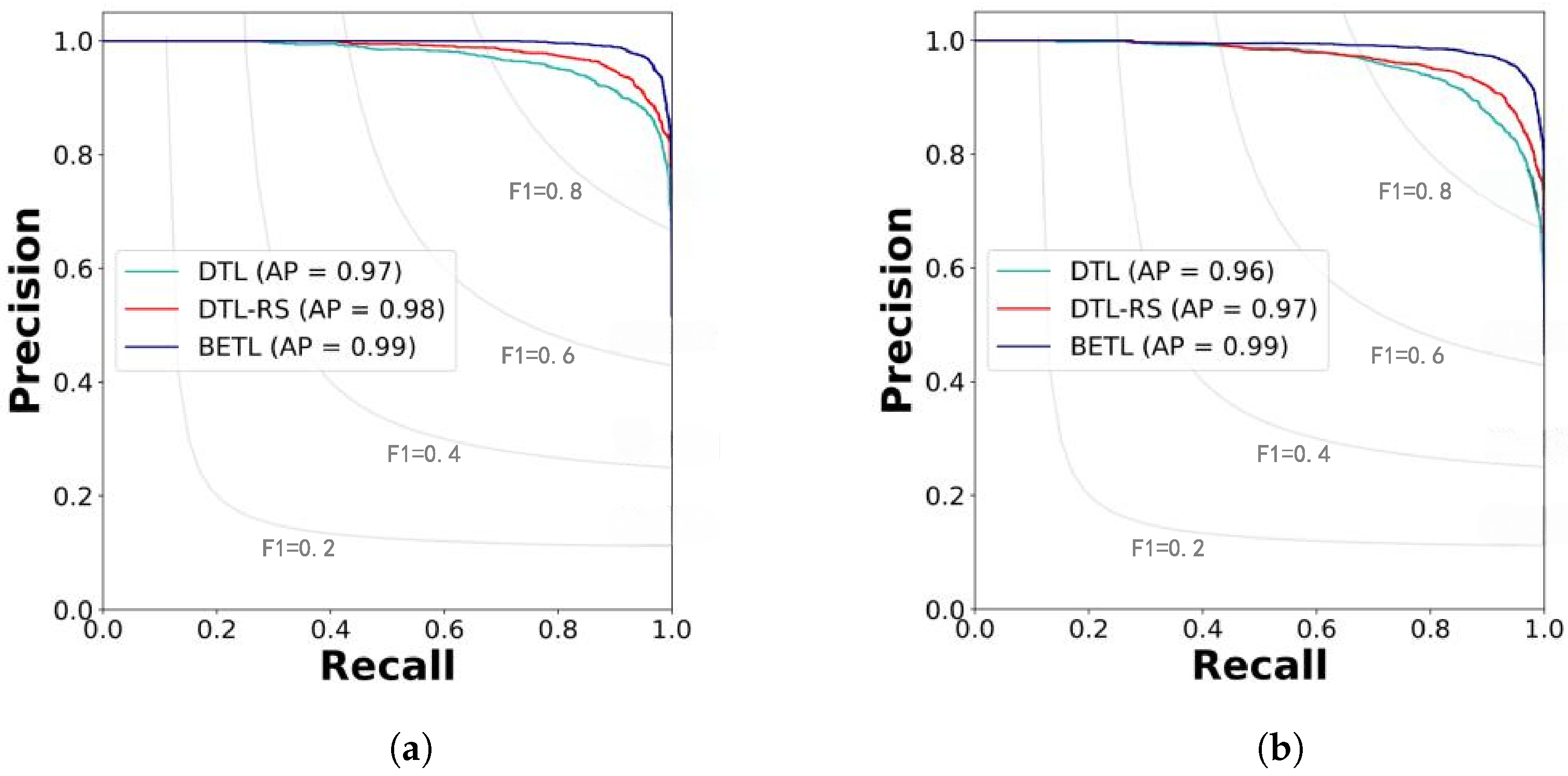
The results in Figure 22 demonstrate that the overall performance of the proposed method is effectively enhanced, with improved recognition performance for scarce classes. The closer the area under the curve for each class is to 1, the better the recognition performance.
The effectiveness of the proposed method in actual scenarios is validated by these findings.
- (2)
- = 5.38
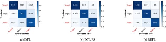
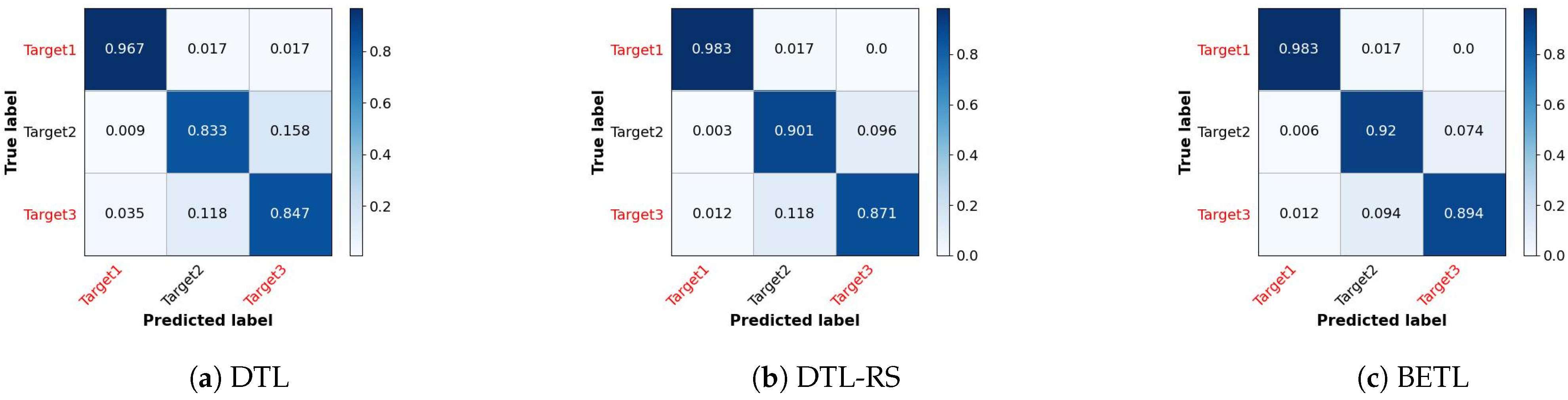
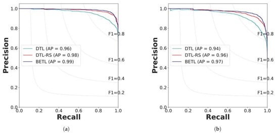
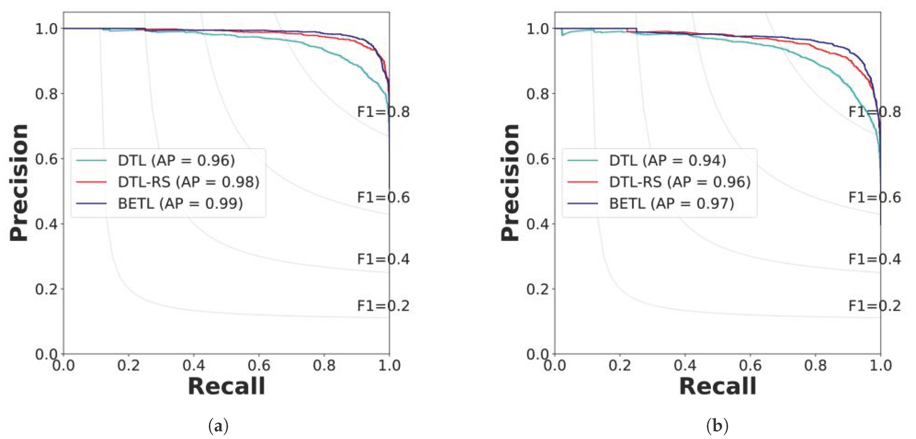
To further validate the effectiveness and generalization of the algorithm proposed in this paper, a new dataset of field test measurements with an imbalance ratio of = 5.38 was introduced. A five-fold cross-validation method was employed, with a total of 144 samples in the balanced subsets (48 samples per class). During the ensemble learning training phase, the number of classifiers used for balancing was set to an integer close to the dataset’s imbalance ratio, i.e., T = 5. The remaining training parameters were kept consistent with those used previously. The confusion matrix for recognition based on the fused feature image dataset under this imbalance ratio is shown in Figure 23, the results are shown in Figure 24, and the specific metric results are presented in Table 13.
Figure 23.
Confusion Matrix Results.
Figure 24.
Results. (a) Results for Target Class with the smallest sample number; (b) overall results for all target classes.
Table 13.
Results of different methods based on the field test dataset.
As shown by the experimental results above, incorporating the resampling strategy improves the recognition accuracy of the three target classes from 96.7%, 83.3%, and 84.7% to 98.3%, 90.1%, and 87.1%, respectively. These overall results are similar to those obtained using data with an imbalance ratio of 4.04 and outperform the accuracy achieved by recognition methods based on deep transfer learning using fused results. The recognition accuracy for Target 2 improved by approximately 6.8%, while that for the scarce class Target 3 improved by approximately 2.4%. Based on the method proposed in this paper, the recognition accuracies for the three underwater target classes are 98.3%, 92.0%, and 89.4%, respectively, with improvements observed for both Target 2 and Target 3. As shown in Table 13, the value obtained using the deep transfer learning method was 0.880; this was improved to 0.917 by combining it with the resampling method, and finally reached 0.932 using the method proposed in this paper; The scores obtained using the three methods were 0.882, 0.918, and 0.933, respectively. Similarly to the experimental results on the underwater target spurious-time–frequency feature fusion dataset with an information ratio () of 4.04, the results in Figure 24 demonstrate that the overall performance of the proposed method has been effectively improved, addressing issues such as insufficient feature information or weak data representation capabilities.
4. Discussion
Due to the challenges of limited feature representation and class imbalance in underwater target recognition, this paper innovatively introduced a LiT-INN dual-branch auto-encoder architecture for feature fusion, as well as proposing a balanced ensemble transfer learning method to reduce the adverse effects of class imbalance. Experimental results based on field test data show that the proposed method achieves excellent performance in underwater target classification tasks. As demonstrated by the experimental comparisons, our method improves the recognition accuracy of underwater targets, especially for classes with few samples, and outperforms conventional deep transfer learning methods in terms of both minority-class accuracy and overall recognition performance.
The primary advantage of this method lies in its superior underwater target recognition performance compared with traditional approaches. Nevertheless, it suffers from higher computational costs and requires expensive GPU resources when handling large-scale datasets and complex model structures. For instance, it requires more training time than baseline models, as shown in Table 14. Future studies may further enhance the model through optimization methods such as meta-learning. In specific application domains, these methods can effectively mitigate the reliance of deep learning on massive datasets for extracting critical classification features. Moreover, expanding the model by increasing the number of parameters may also improve its performance across different datasets.
Table 14.
Training time comparison.
5. Conclusions
This paper proposed an underwater target recognition method based on feature fusion and balanced ensemble transfer learning. By addressing both feature representation capabilities and network training approaches, it resolves the issues of weak feature representation in single time–frequency feature images and poor recognition performance caused by class imbalance. This provides a new, effective pathway for solving underwater target recognition problems in complex environments. First, a LiT-INN dual-branch auto-encoder architecture was employed for time–frequency image feature fusion. The Restormer network served as a shared feature encoder to extract foundational features, enabling feature fusion of underwater target echo time–frequency image data and generating a fusion dataset with richer feature information. Second, a balanced ensemble transfer learning method was constructed based on a two-stage decoupled fine-tuning learning method. The first stage employed a uniform sampler strategy to fine-tune the feature extraction module of the pre-trained transfer learning model. The second stage utilized a multiple-balanced-sampling optimization method to fine-tune the classifier. Then, a weight averaging ensemble learning method was adopted to fuse multiple weak classifiers at the decision level.
Field test echo time–frequency data covering three classes of underwater targets demonstrate that when = 4.04, using the deep transfer learning method, the average underwater target recognition accuracy for the class with the fewest samples reaches 0.97, while the overall average recognition accuracy achieves 0.96. Through the proposed method, the average recognition accuracy for the class with the fewest samples reaches 0.99, and the overall recognition accuracy reaches 0.99, demonstrating superior performance compared to the deep learning transfer learning method and validating the effectiveness of the proposed approach. When = 5.38, using the deep transfer learning method, the average underwater target recognition accuracy for the class with the fewest samples reaches 0.96, while the overall average recognition accuracy achieves 0.94. Through the proposed method, the average recognition accuracy for the class with the fewest samples reaches 0.99, and the overall recognition accuracy reaches 0.97, further validating the effectiveness and generalization of the proposed approach. The proposed method effectively improves recognition performance for target classes with few samples and significantly enhances overall recognition accuracy.
Despite enhancing active sonar recognition performance, the proposed method has certain limitations. For instance, its adaptability and efficiency for class imbalance optimization require improvement. Future work will explore more adaptive and efficient class imbalance optimization methods, such as integrating meta-learning to optimize recognition performance for target classes with fewer samples. Though the recognition system performs well in static scenarios, it could struggle with real-world dynamic conditions. As a result, the real dynamic motion of targets (e.g., target velocity and acceleration, Doppler effect) will be an essential part of future work.
Author Contributions
Data curation, H.Z.; methodology, H.Z.; project administration, H.L.; software, H.Z.; supervision, H.L.; validation, L.Z. and W.G.; writing—original draft, H.Z.; writing—review and editing, H.L., L.Z. and W.G. All authors have read and agreed to the published version of the manuscript.
Funding
This research was funded by the National Natural Science Foundation of China under grant number 62371394.
Data Availability Statement
The data presented in this study are available on request from the corresponding author due to privacy.
Conflicts of Interest
The authors declare no conflicts of interest.
Abbreviations
The following abbreviations are used in this manuscript:
| MFCC | Mel Frequency Cepstrum Coefficient |
| SNR | Signal-to-Noise Ratio |
| LOFAR | Low-Frequency Analysis and Recording |
| LiT | Lite-Transformer |
| INN | Invertible Neural Networks |
| SSIM | Structural Similarity Index |
| TL | Transfer Learning |
| LFM | Linear Frequency Modulation |
| Imbalance Ratio | |
| CH | Calinski–Harabasz Score |
| DB | Davies–Bouldin Index |
| DTL | Deep Transfer Learning Method |
| DTL-RS | Resampling Deep Transfer Learning |
| BETL | Balanced Ensemble Transfer Learning (this paper) |
References
- Luo, X.; Chen, L.; Zhou, H.; Cao, H. A survey of underwater acoustic target recognition methods based on machine learning. J. Mar. Sci. Eng. 2023, 11, 384. [Google Scholar] [CrossRef] [Scilit]
- Fang, S.; Du, S.; Luo, X.; Han, N.; Xu, X. Development of underwater acoustic target feature analysis and recognition technology. Bull. Chin. Acad. Sci. (Chin. Version) 2019, 34, 297–305. [Google Scholar]
- Erol-Kantarci, M.; Mouftah, H.T.; Oktug, S. A survey of architectures and localization techniques for underwater acoustic sensor networks. IEEE Commun. Surv. Tutor. 2011, 13, 487–502. [Google Scholar] [CrossRef] [Scilit]
- Lei, Z.; Lei, X.; Wang, N.; Zhang, Q. Present status and challenges of underwater acoustic target recognition technology: A review. Front. Phys. 2022, 10, 1044890. [Google Scholar] [CrossRef] [Scilit]
- Kenny, A.J.; Cato, I.; Desprez, M.; Fader, G.; Schüttenhelm, R.T.E.; Side, J. An overview of seabed-mapping technologies in the context of marine habitat classification. ICES J. Mar. Sci. 2003, 60, 411–418. [Google Scholar] [CrossRef] [Scilit]
- Testolin, A.; Kipnis, D.; Diamant, R. Detecting submerged objects using active acoustics and deep neural networks: A test case for pelagic fish. IEEE Trans. Mob. Comput. 2020, 21, 2776–2788. [Google Scholar] [CrossRef] [Scilit]
- Testolin, A.; Diamant, R. Combining denoising autoencoders and dynamic programming for acoustic detection and tracking of underwater moving targets. Sensors 2020, 20, 2945. [Google Scholar] [CrossRef] [Scilit]
- Yuan, F.; Ke, X.; Cheng, E. Joint representation and recognition for ship-radiated noise based on multimodal deep learning. J. Mar. Sci. Eng. 2019, 7, 380. [Google Scholar] [CrossRef] [Scilit]
- Sun, Z.; Jiang, J.; Li, Y.; Wang, X.; Li, C.; Li, Z.; Miao, Y.; Fu, X.; Duan, F. Bio-inspired covert active sonar detection method based on the encoding of sperm whale clicks. IEEE Sens. J. 2021, 22, 1449–1460. [Google Scholar] [CrossRef] [Scilit]
- Chen, Y.; Liang, H.; Pang, S. Study on small samples active sonar target recognition based on deep learning. J. Mar. Sci. Eng. 2022, 10, 1144. [Google Scholar] [CrossRef] [Scilit]
- Korany, N. Application of wavelet transform for classification of underwater acoustic signals. Proc. Mtgs. Acoust. 2016, 28, 070003. [Google Scholar]
- Ou, H.H.; Au, W.W.; Syrmos, V.L. Underwater ordnance classification using time-frequency signatures of backscattering signals. In Proceedings of the Oceans 2010 MTS/IEEE Seattle, Seattle, WA, USA, 20–23 September 2010; IEEE: New York, NY, USA, 2010; pp. 1–8. [Google Scholar]
- Zeng, S.; Du, X. Multimodal underwater target recognition method based on deep learning. J. Appl. Acoust. 2019, 38, 589–595. [Google Scholar]
- Dong, W.; Fu, J.; Wang, X.; Shen, Z. Underwater Acoustic Target Feature Fusion Recognition Using Multitask Learning. In Proceedings of the 2024 OES China Ocean Acoustics (COA), Harbin, China, 29–31 May 2024; IEEE: New York, NY, USA, 2024; pp. 1–5. [Google Scholar]
- Yang, Y.; Yao, Q.; Wang, Y. Underwater Acoustic Target Recognition Method Based on Feature Fusion and Residual CNN. IEEE Sens. J. 2024, 24, 37342–37357. [Google Scholar] [CrossRef] [Scilit]
- Hu, Z.; Li, H.; Tang, Z.; Wang, X.; Sun, J.; Quan, D. Radar Signal Recognition Based on Deep Feature Fusion of Multiple Time-frequency Images. In Proceedings of the 2023 International Conference on Wireless Communications and Signal Processing (WCSP), Hangzhou, China, 2–4 November 2023; IEEE: New York, NY, USA, 2023; pp. 377–383. [Google Scholar]
- LeCun, Y.; Bengio, Y.; Hinton, G. Deep learning. Nature 2015, 521, 436–444. [Google Scholar] [CrossRef] [Scilit]
- Dong, Y.; Shen, X.; Jiang, Z.; Wang, H. Recognition of imbalanced underwater acoustic datasets with exponentially weighted cross-entropy loss. Appl. Acoust. 2021, 174, 107740. [Google Scholar] [CrossRef] [Scilit]
- Pang, Y.; Wu, C.; Wu, H.; Yu, X. Over-sampling strategy-based class-imbalanced salient object detection and its application in underwater scene. Vis. Comput. 2023, 39, 1959–1974. [Google Scholar] [CrossRef] [Scilit]
- Wang, Y.X.; Ramanan, D.; Hebert, M. Learning to Model the Tail. In Proceedings of the Advances in Neural Information Processing Systems; Curran Associates, Inc.: Red Hook, NY, USA, 2017; Volume 30, pp. 7029–7039. [Google Scholar]
- Chen, L.; Yu, H.; Dong, X.; Li, Y.; Shen, J.; Shen, J.; Xu, Q. BAUODNET for Class Imbalance Learning in Underwater Object Detection. IEEE Trans. Emerg. Top. Comput. Intell. 2025, 9, 2452–2461. [Google Scholar] [CrossRef] [Scilit]
- Zamir, S.W.; Arora, A.; Khan, S.; Hayat, M.; Khan, F.S.; Yang, M.H. Restormer: Efficient transformer for high-resolution image restoration. In Proceedings of the 2022 IEEE/CVF Conference on Computer Vision and Pattern Recognition (CVPR), New Orleans, LA, USA, 18–24 June 2022; IEEE: New York, NY, USA, 2022; pp. 5728–5739. [Google Scholar]
- Wu, Z.; Liu, Z.; Lin, J.; Lin, Y.; Han, S. Lite Transformer with Long-Short Range Attention. arXiv 2020, arXiv:2004.11886. [Google Scholar] [CrossRef] [Scilit]
- Ardizzone, L.; Kruse, J.; Wirkert, S.; Rahner, D.; Pellegrini, E.W.; Klessen, R.S.; Maier-Hein, L.; Rother, C.; Köthe, U. Analyzing Inverse Problems with Invertible Neural Networks. arXiv 2019, arXiv:1808.04730. [Google Scholar] [CrossRef] [Scilit]
- Yanchin, I.; Guedes Soares, C. Gradient Boosted Trees and Denoising Autoencoder to Correct Numerical Wave Forecasts. J. Mar. Sci. Eng. 2024, 12, 1573. [Google Scholar] [CrossRef] [Scilit]
- Michelucci, U. An introduction to autoencoders. arXiv 2022, arXiv:2201.03898. [Google Scholar] [CrossRef] [Scilit]
- Tao, W.; Luo, Y.; Tong, J.; Xia, Q.; Qu, J. A Ship Heading Estimation Method Based on DeepLabV3+ and Contrastive Learning-Optimized Multi-Scale Similarity. J. Mar. Sci. Eng. 2025, 13, 1085. [Google Scholar] [CrossRef] [Scilit]
- Buda, M.; Maki, A.; Mazurowski, M.A. A systematic study of the class imbalance problem in convolutional neural networks. Neural Netw. 2018, 106, 249–259. [Google Scholar] [CrossRef] [Scilit]
- Ganaie, M.A.; Hu, M.; Malik, A.K.; Tanveer, M.; Suganthan, P.N. Ensemble deep learning: A review. Eng. Appl. Artif. Intell. 2022, 115, 105151. [Google Scholar] [CrossRef] [Scilit]
- Hazarika, N.; Chen, J.Z.; Tsoi, A.C.; Sergejew, A. Classification of EEG signals using the wavelet transform. Signal Process. 1997, 59, 61–72. [Google Scholar] [CrossRef] [Scilit]
- Nawab, S.H.; Quatieri, T.F. Short-time Fourier transform. In Advanced Topics in Signal Processing; Prentice-Hall, Inc.: Hoboken, NJ, USA, 1987; pp. 289–337. [Google Scholar]
- Sun, F.; Wang, M.; Xu, Q.; Xuan, X.; Zhang, X. Acoustic scene recognition based on convolutional neural networks. In Proceedings of the 2019 IEEE 4th International Conference on Signal and Image Processing (ICSIP), Wuxi, China, 19–21 July 2019; IEEE: New York, NY, USA, 2019; pp. 122–126. [Google Scholar]
- Andria, G.; Savino, M. Interpolated smoothed pseudo Wigner-Ville distribution for accurate spectrum analysis. IEEE Trans. Instrum. Meas. 2002, 45, 818–823. [Google Scholar] [CrossRef] [Scilit]
- He, K.; Zhang, X.; Ren, S.; Sun, J. Deep Residual Learning for Image Recognition. In Proceedings of the 2016 IEEE Conference on Computer Vision and Pattern Recognition (CVPR), Las Vegas, NV, USA, 27–30 June 2016; IEEE: New York, NY, USA, 2016; pp. 770–778. [Google Scholar]





Disclaimer/Publisher’s Note: The statements, opinions and data contained in all publications are solely those of the individual author(s) and contributor(s) and not of MDPI and/or the editor(s). MDPI and/or the editor(s) disclaim responsibility for any injury to people or property resulting from any ideas, methods, instructions or products referred to in the content. |
© 2026 by the authors. Licensee MDPI, Basel, Switzerland. This article is an open access article distributed under the terms and conditions of the Creative Commons Attribution (CC BY) license.