A Remote Sensing Monitoring System for Marine Red Tides Based on Targeted Negative Sample Selection Strategies

Abstract

The monitoring of harmful algal blooms (HABs) constitutes a vital component of marine environmental protection and the sustainable development of the marine economy. However, the highly dynamic nature of these small targets, compounded by the complex water color interference prevalent in the coastal waters where HABs frequently occur, has resulted in traditional remote sensing monitoring methods, particularly those relying on fixed spectral index thresholds and pixel-wise binarization, suffering from imprecise identification in turbid coastal waters where suspended sediments, cloud cover, and sun glint create spectral confusion. These methods also exhibit low automation due to manual threshold adjustment requirements and poor transferability across different spatiotemporal conditions. Consequently, these methods struggle to meet practical application requirements. This study establishes a U-net model-based remote sensing identification framework for red tides using HY-1D CZI imagery (50 m resolution, 1–3 day revisit), targeted negative sample strategies, and event-level accuracy validation methods to achieve efficient marine red tide detection. Targeted negative sample selection involves purposefully selecting spectrally ambiguous regions as negative samples, aiming to enhance recognition accuracy and sample selection efficiency. The combination of targeted sampling with deep learning enables portability to new spatiotemporal contexts by learning invariant spectral–spatial features rather than relying on scene-specific thresholds. Experimental results demonstrate that the targeted negative sample strategy reduces event-level model false negatives by 27%, false positives by 36%, and increases the F1 score by 0.3217. Using an identical sample size, the targeted sample selection strategy yields an F1 score 0.0479 higher than random sampling. To achieve equivalent recognition accuracy, an increased number of random samples would be required. Comparative experiments reveal that the proposed method enhances sample selection efficiency by 87.5%. Transferability is demonstrated through successful identification of red tide patches in Wenzhou waters on 13 April 2022, without model retraining. This demonstrates that red tide remote sensing recognition based on targeted sample selection enables efficient, precise, and automated identification without human intervention, providing a reliable technical solution for operational marine red tide monitoring.

1. Introduction

Red tides, as an ecological anomaly triggered by the explosive proliferation of phytoplankton, pose a severe threat to the health of global coastal ecosystems, aquaculture industries [1], and public safety when occurring frequently [2]. Red tide disasters typically unfold as dynamic processes, drifting and spreading with tidal currents, runoff, and sea winds [3]. Without effective short-term mitigation measures, such as physical barriers or aquaculture relocation, they can inflict widespread ecological damage. To enable timely intervention, accurate and rapid spatial positioning of red tide patches is paramount, making reliable monitoring technologies crucial for informing mitigation decisions. Traditional in situ observation methods and mechanistic modeling approaches prove inadequate for obtaining relatively precise, real-time spatial distributions of red tide blooms. Consequently, developing large-scale, rapid, and accurate red tide identification techniques holds significant scientific value and practical necessity. Scientifically, such techniques enable investigation of bloom dynamics, transport mechanisms, and ecosystem responses across spatial scales that cannot be captured by point-based sampling. Practically, they support early warning systems for aquaculture operations, coastal tourism management, and public health advisories—applications that require timely and spatially explicit information to guide decision-making. Satellite remote sensing, leveraging its macro-scale, real-time, and periodic observation advantages, can capture relatively accurate spatial distributions of red tides and has become an indispensable tool for dynamic red tide identification [4].

In this study, we define “red tide” operationally as the visible manifestation of harmful algal blooms (HABs) in satellite imagery. In remote sensing imagery, red tide targets manifest as small-scale patches with blurred boundaries and irregular striped patterns, exhibiting highly dynamic characteristics. Concurrently, sedimentation, wave action, and fluctuating water coloration in nearshore areas prone to red tides significantly impede their identification. In remote sensing interpretation studies, high-resolution imagery such as Sentinel-2 [5,6] or GF (Gaofen) series [7] is typically employed for small-scale targets. However, such high-resolution imagery often has extended revisit periods, failing to meet the monitoring requirements for highly dynamic red tides. Conversely, studies targeting highly dynamic phenomena typically employ imagery with shorter revisit cycles, such as MODIS, yet its lower spatial resolution fails to capture small-scale red tide patches. This creates a fundamental trade-off: no single sensor simultaneously provides both high spatial and high temporal resolution. Therefore, data selection must prioritize based on event characteristics: for rapidly evolving blooms, temporal resolution takes precedence, but sufficient spatial resolution must be retained to resolve patch structure. In this study, we selected HY-1D CZI imagery (50 m resolution, 1–3 day revisit) as the best available compromise for monitoring dynamic red tides in coastal waters.

Regarding methods for interpreting red tides, current optical remote sensing-based identification predominantly relies on the calculation and analysis of specific spectral indices—transformations of reflectance data designed to enhance algal signals [8]. However, while these indices provide useful feature representations, they must be coupled with decision rules to produce final classifications. The most common approach—threshold segmentation—faces multiple challenges in practical application. Among spectral indices for algal bloom detection, NDVI is sensitive to vegetation signals but suffers from atmospheric and glint interference in aquatic environments [9]. The Floating Algae Index (FAI) improves upon NDVI by using a baseline subtraction method yet remains susceptible to turbid water effects in coastal zones [10]. The VB-FAH index, proposed by Hu [11], constructs a virtual baseline using green and red bands to calculate the ‘height’ of the near-infrared reflectance. This approach effectively suppresses interference from aerosols, sun glint, and variable observation geometry, making it particularly suitable for turbid coastal waters where suspended sediments and dynamic water color frequently confound other indices. While alternative approaches exist, such as machine learning classifiers or object-based image analysis, threshold-based segmentation of spectral indices remains prevalent in operational red tide monitoring due to its simplicity and interpretability. However, this traditional approach involving index calculation and threshold segmentation faces multiple challenges in practical application. Firstly, threshold determination heavily relies on expert judgement and specific image conditions [8]. Image brightness is influenced by multiple factors including solar elevation angle, atmospheric conditions, and sea surface roughness. This variability makes it difficult to establish a fixed, uniform threshold for a single image, often necessitating cumbersome manual adjustments for each individual image, resulting in very low automation levels. Secondly, spectral characteristics of non-red tide features—such as cloud cover, solar glare, and high-concentration suspended sediments—often overlap with red tide areas, creating “mixed pixels”. This causes pixel-based thresholding methods to generate numerous false alarms, a problem particularly pronounced in turbid coastal waters [8,11,12]. Moreover, traditional methods fail to effectively utilize spatial contextual information within imagery, struggling to distinguish between objects exhibiting spectral similarity at the pixel level yet differing in spatial patterns [13]—termed “spectrally identical objects with distinct spatial patterns”. Conversely, regions with identical red tides at different spatio-temporal points may exhibit divergent spectral characteristics in remote sensing imagery—known as “identical objects with distinct spectral signatures”. Based on these considerations, we hypothesize that: (1) guided by VB-FAH, targeted selection of spectrally ambiguous non-red tide areas (clouds, sediments, glint, shallow transitions) as negative samples will enable the U-Net model to learn discriminative features that reduce false positives in complex coastal environments; (2) this targeted approach will require substantially fewer negative samples than random sampling to achieve equivalent recognition accuracy, thereby improving sample selection efficiency.

In recent years, deep learning, particularly fully convolutional networks, has achieved revolutionary progress in the semantic segmentation of remote sensing imagery [14]. Models such as U-Net, with their encoder–decoder architecture and skip connections, successfully extract high-level semantic features while preserving detail information. They have been applied to tasks including land cover classification and building extraction [15], offering novel insights for red tide identification. Specifically, through training, models can directly learn the complex spatial–spectral characteristics of red tides from imagery, potentially enabling end-to-end automated extraction. Han et al. enhanced the U-Net model by incorporating NDVI as an augmenting feature, significantly improving detection accuracy for red tide boundaries [16]. However, existing research generally overlooks the critical impact of negative samples on model generalization, resulting in persistently high false alarm rates in complex scenarios [17]. Some studies employ random sampling or simplistic segmentation to construct negative samples [18]. This approach fails to enable models to learn specifically to distinguish blooms from easily confused confounding elements (such as thin clouds, broken wave foam, or turbid water edges). Consequently, models may perform well on training datasets but exhibit insufficient robustness when confronted with the variable disturbances encountered in real environments [19]. Furthermore, studies identifying morphologically similar microalgae have revealed that the presence of interfering species directly causes a significant decline in model recognition accuracy [20,21], indirectly underscoring the importance of handling interference samples. Consequently, constructing a training dataset that guides the model to focus on learning “difficult-to-distinguish” features is imperative for enhancing the model’s practical application performance.

Moreover, accuracy assessment for red tide detection faces unique challenges. Traditional remote sensing accuracy evaluation relies on pixel-by-pixel comparison with independently collected ground truth data. However, for red tides, obtaining synchronous ground truth is difficult: the highly dynamic nature means that by the time a sampling vessel reaches a location, the bloom may have drifted or dissipated. Furthermore, red tide patches have inherently fuzzy boundaries, making it challenging to delineate clear edges even through visual interpretation. To address this, we introduce an event-level validation approach that evaluates detection at the patch scale rather than the pixel scale, focusing on whether blooms are identified rather than exact boundary delineation.

In summary, addressing the aforementioned issues, this study has established a practical red tide identification system. Regarding remote sensing data selection, the study comprehensively considered spatio-temporal resolution, opting for HY-1D satellite imagery. This choice enables observation of red tide morphology while providing sufficient temporal resolution for interpreting dynamic red tides. To enhance the interpretability of the model, this study proposes an automated red tide recognition framework based on the U-Net architecture and a targeted sample selection strategy. This approach overcomes the limitations of random sampling by leveraging the physical significance of the VB-FAH index to precisely identify various types of red tide patches. It further selects spectrally or spatially ambiguous interference samples from non-red tide areas—those prone to confusion with red tides—and incorporates them into the training set. This aims to actively “train” the model to distinguish these challenging cases, thereby enhancing the model’s discriminative power and robustness at the data level. Regarding the construction of remote sensing evaluation methods for red tide disasters, this paper designs an event-level accuracy verification method based on the characteristics of red tides and their backgrounds. This approach overcomes the issue of excessively low pixel-level verification accuracy in traditional remote sensing interpretation. Integrating the comprehensive red tide identification system, this research has developed a monitoring technology framework exhibiting low false alarm rates, low missed detection rates, and strong practicality in complex environments. This provides a novel solution to advance red tide remote sensing identification from “manual threshold intervention” towards “fully automated intelligent recognition”.

2. Materials and Methods

2.1. Research Area

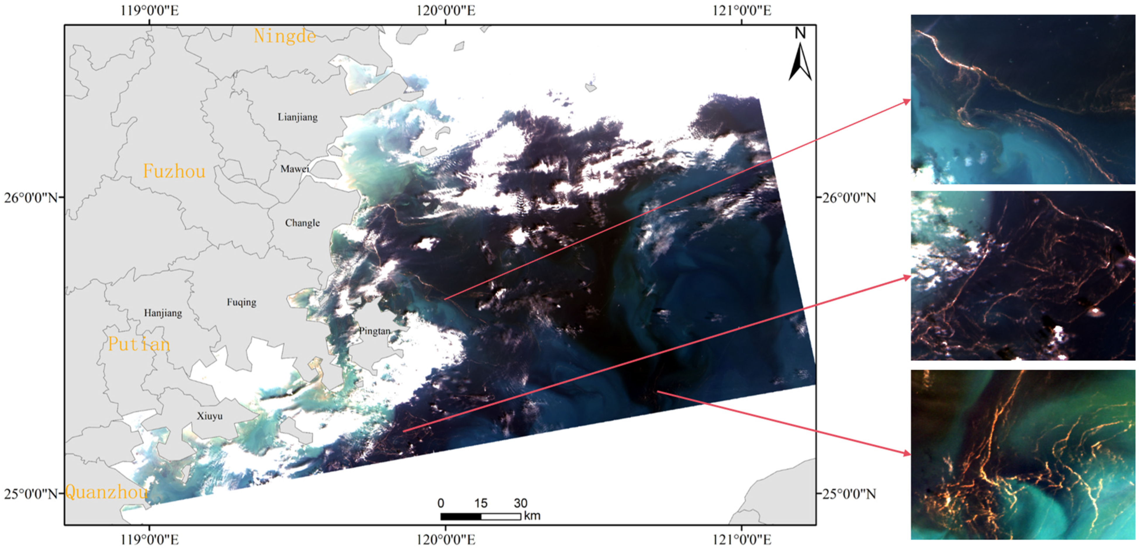
To identify suitable study areas and corresponding satellite imagery, we consulted multiple sources documenting red tide events: the China Marine Disaster Bulletin (2000–2023), event records from the Fujian Provincial Oceanic and Fishery Bureau (2022–2025), and the Guangdong Provincial Marine Disaster Bulletin (2013–2023). These records served as a data discovery tool, providing event dates and approximate locations to guide satellite image acquisition. Based on this screening, we selected the waters near Changle District and Pingtan County in Fuzhou City, Fujian Province, as the study area (Figure 1). This region was chosen because: (1) it has documented frequent red tide events (e.g., the 23–27 April 2022 event used in this study), (2) multiple HY-1D images with <30% cloud cover were available covering these events, and (3) the coastal waters exhibit the spectral complexities (suspended sediments, variable turbidity) that challenge traditional monitoring methods.

Table 1. Excerpt from the 2022 China Marine Disaster Bulletin [22].

Province	Start and End Times	Discovery Zone	Area (km2)	Data Can Be Collected or Not	Red Tides Observed or Not
Zhejiang	4.10–4.15	Wenzhou marine waters	533	Yes	Yes
Fujian	4.23–4.27	Pingtan, Liushui, Baiqing, Suao and other areas	120	Yes	Yes
Zhejiang	5.6–5.23	Da Chen Sea Area, Jiaojiang District, Taizhou	120	No	No
Zhejiang	5.10–5.24	The marine waters from Pishan Island, Yuhuan, Taizhou to Wenling	200	No	No
Fujian	6.1–6.9	The marine waters near Dongdai and Kengkou, Nanri Island, Putian	40	Yes	No
Fujian	6.10–6.13	Pingtan, Liushui, Suao and other areas	10	No	No
Zhejiang	7.25–8.4	The marine waters south of Dachangtu Island and Daxizhai Island, Daishan	100	No	No
Zhejiang	7.26–8.5	The marine waters east of Zhujiajian, Taohua Island and Xiazhi Island in Putuo District, Zhoushan	250	No	No

is excerpted from the 2022 China Marine Disaster Bulletin. The table indicates that among red tide events occurring within the southeastern coastal region, only three scenes of imagery were screened as covering this area, with only two scenes showing observable red tides.

This study selected the waters near Changle District and Pingtan County [23] in Fuzhou City, Fujian Province, as the study area (Figure 1), conducting experiments using the disaster event occurring between 23 and 27 April 2022 as an example.

2.2. Method

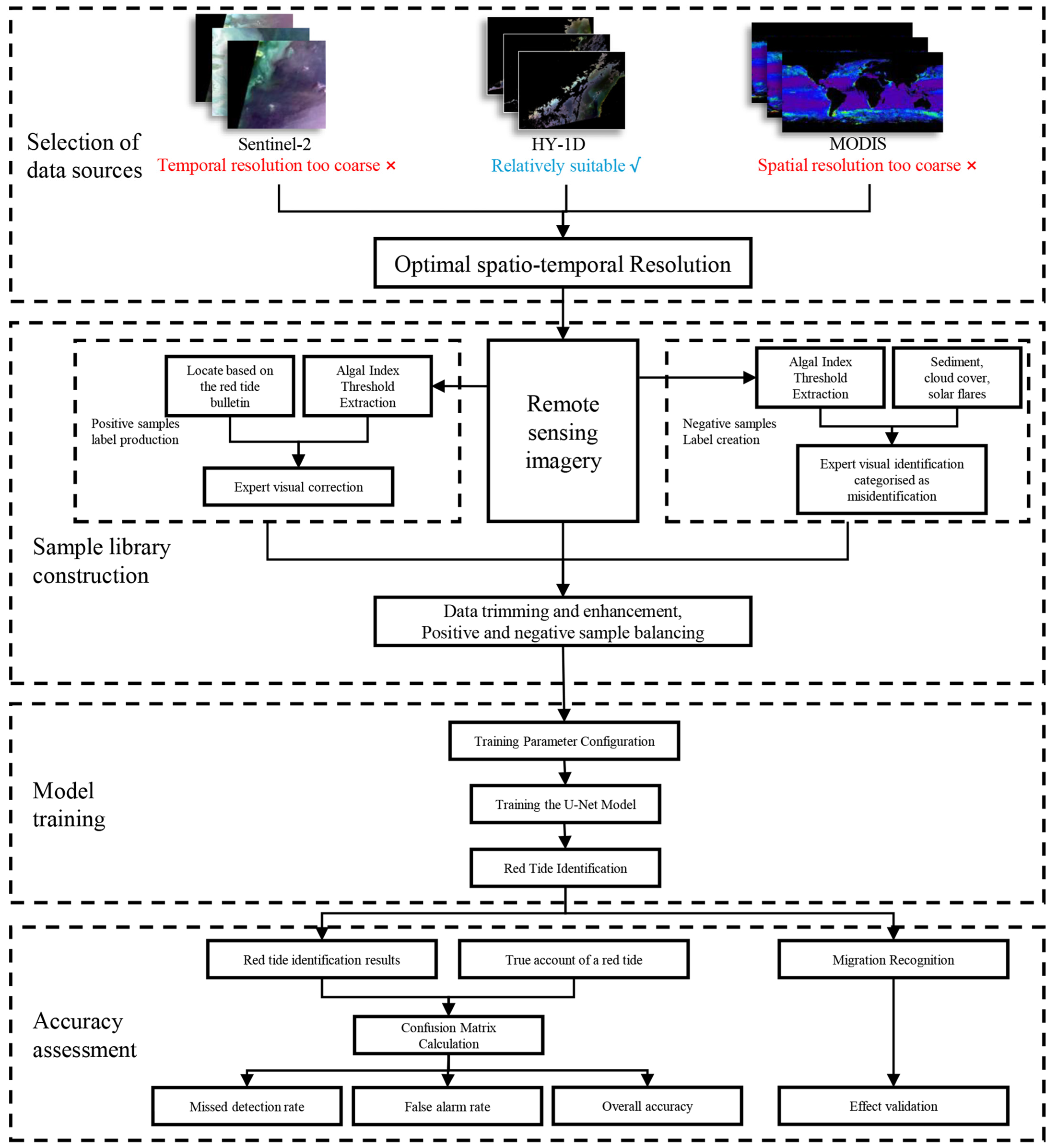
The overall workflow comprises data source selection, sample repository construction, model architecture and training, and accuracy assessment. Addressing the challenge of obtaining high-quality remote sensing imagery for red tides, this study compared various spatio-temporal resolution remote sensing data sources to identify the most suitable satellite data for red tide research. Specific red tide occurrence times and locations were identified using the China Marine Disaster Bulletin, enabling the selection of corresponding remote sensing imagery. Data underwent processing, employing targeted sample selection strategies to create sample labels and remote sensing image tiles for constructing the sample repository. A U-Net deep learning model was utilized for red tide recognition. To accurately evaluate disaster recognition performance, an event-level accuracy validation method was introduced, enabling comprehensive precision assessment. The detailed workflow is illustrated in Figure 2.

2.2.1. Data Source Selection

Given the characteristics of algal blooms, high-resolution imagery such as Sentinel-2 is commonly employed for their interpretation. With its 10-m resolution, it can finely delineate the morphology of blooms. However, its temporal resolution is relatively low, featuring a revisit cycle of 3–10 days. This cycle frequently spans the entire duration of a single bloom event. Among the high-quality imagery from multiple satellites examined, no continuous time-series data is available, rendering it unsuitable for studying highly dynamic algal blooms. The collected MODIS data features a one-day revisit cycle, offering high temporal resolution. However, daily Level-3 products have a spatial resolution of 4 km, with each pixel covering approximately 16 km², making it difficult to accurately reflect small-scale bloom patches. To address these spatio-temporal resolution limitations, this study employs HY-1D CZI satellite imagery [24,25]. As an independently developed ocean color remote sensing satellite of China, HY-1D was launched in September 2020, equipped with payloads such as the Coastal Zone Imager (CZI) and the Chinese Ocean Color and Temperature Scanner (COCTS). It has the ability of ocean observation with high spatial and temporal resolution, which can realize refined and normalized monitoring of China’s coastal waters and is an important data source for remote sensing monitoring of the marine ecological environment. Its spatial resolution is 50 m with a revisit cycle of 1–3 days, spanning the period from 2020 to 2025, making it suitable for monitoring highly dynamic red tides. Compared to the COCTS satellite, although it offers more monitoring bands, its 1.1 km resolution remains too low. Conversely, the CZI’s monitoring of red, green, blue, and near-infrared bands precisely covers the key spectral range for red tide identification. Its high 50 m spatial resolution provides a distinct advantage, making it suitable for coastal environmental monitoring [25]. Regarding the HY-1D-CZI image library, although L1B-level imagery reflects true color, the limited availability of usable images within the study area precludes its application for dynamic red tide research. Consequently, this study employs L2A-level imagery, with all images undergoing atmospheric and geometric correction [26]. The spatio-temporal resolutions of each data source are detailed in

Table 2. Spatial and temporal resolution of various data source.

		HY-1D CZI	HY-1D COCTS	Sentinel-2	MODIS	Landsat-8/9 OLI
Spatial resolution		50 m	1100 m	10 m	4000 m	30 m
Revisit cycle		1–3 day	1–3 day	3–10 day	1–2 day	16 day
Center Wavelength	Blue	460 nm	443 nm	490 nm	469 nm	482 nm
	Green	560 nm	555 nm	560 nm	555 nm	561 nm
	Red	650 nm	670 nm	665 nm	645 nm	655 nm
	NIR	825 nm	865 nm	842 nm	858 nm	865 nm
Cloud-free Scenes		45%	32.6%	49%	11.9%	20%
Suitability		Optimal compromise	Temporal resolution too coarse	Temporal resolution too coarse	Spatial resolution too coarse	Temporal resolution too coarse

.

2.2.2. Sample Library Construction

Red Tide Label Production

Due to spectral differences between red tides and seawater, red tide outbreaks cause changes in water coloration. This study employs the VB-FAH spectral index (Virtual Baseline Floating macroalgae Height Index) to detect red tides, as it is well-suited for characterizing such phenomena. The VB-FAH index is a specialized algorithm for identifying and quantifying floating macroalgae (such as green tides, Sargassum, and cyanobacterial blooms) in optical remote sensing imagery. It constructs a virtual baseline using the green, red, and near-infrared bands, calculating the ‘height’ of the near-infrared band relative to this baseline (i.e., the VB-FAH value). This height is sensitive to algal signals while exhibiting strong suppression capabilities against interference from atmospheric aerosols, solar glare, and observation geometry. It enables highly robust identification of floating large algae alongside integrated estimation of coverage and biomass, finding widespread application in floating algal identification [11]. The VB-FAH calculation formula is:

$$VB-FAH=(R_4-R_2)+(R_2-R_3)\times {\displaystyle \frac{({\lambda }_4-{\lambda }_2)}{(2{\lambda }_4-{\lambda }_3-{\lambda }_2)}}$$

(1)

R₂, R₃, and R₄ denote the surface reflectance values for the green, red, and near-infrared bands respectively, whilst λ₂ (green band) = 560 nm, λ₃ (red band) = 650 nm, λ₄ (near-infrared band) = 865 nm, which are the central wavelengths of the corresponding bands of HY-1D CZI sensor. This formulation follows Hu’s original VB-FAH definition [11], designed to minimize atmospheric and glint interference through virtual baseline subtraction.

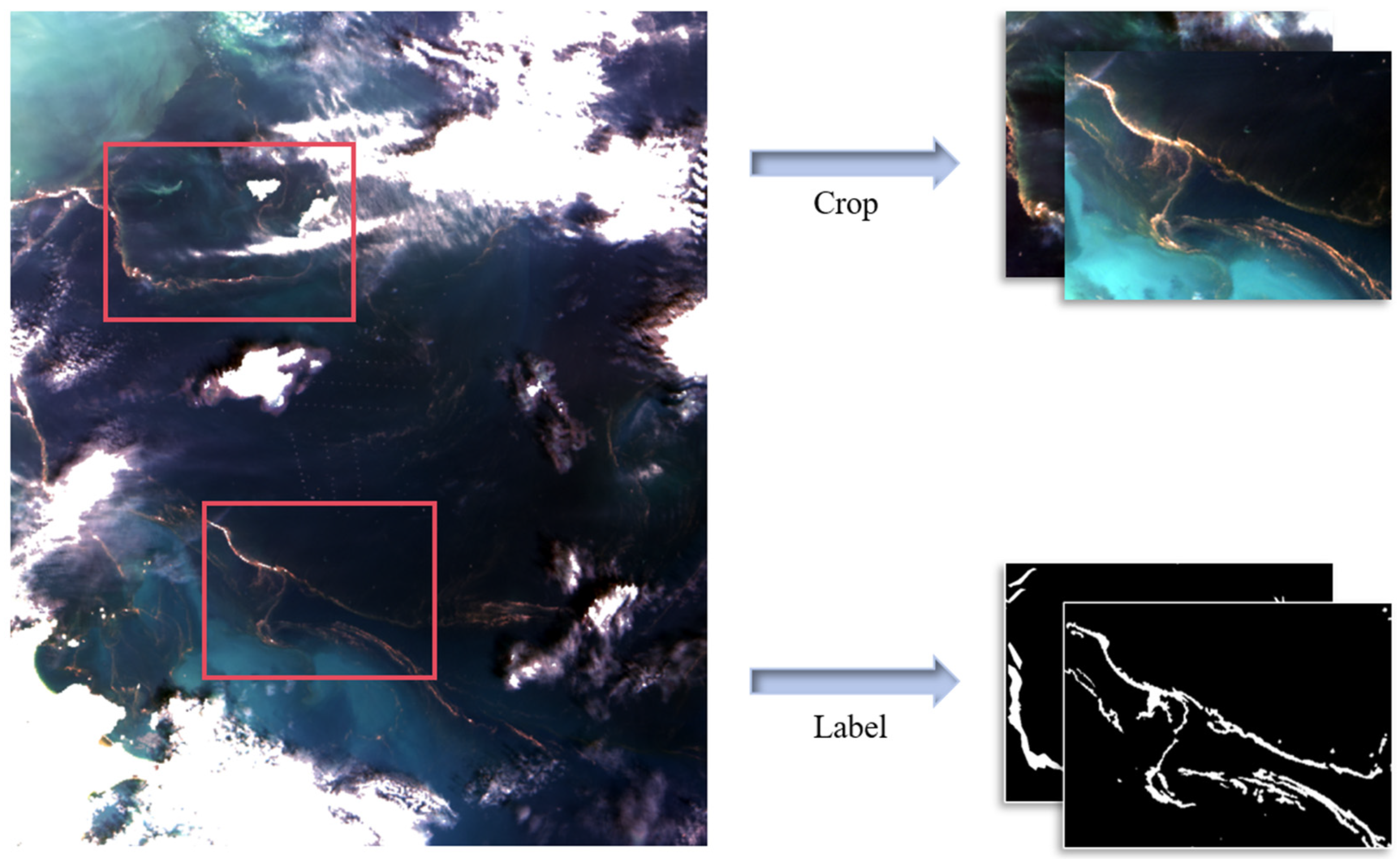
High-resolution ocean satellite imagery was employed to extract the VB-FAH index, which was then integrated with bulletin data to observe red tide outbreak regions. Label features were determined based on the visual characteristics of red tide patches demonstrated in Zhao et al.’s study [24] utilizing HY-1D satellite remote sensing imagery for red tide detection. Thresholds were adjusted to enable the extracted segments to delineate red tide patches with reasonable accuracy. Expert visual interpretation was then employed to manually supplement or refine details, precisely delineating the red tide patch areas. This generated a binary label map (red tide = 1, non-red tide = 0), as illustrated in Figure 3. This approach of combining automated extraction with manual refinement for label creation is widely adopted in remote sensing sample annotation [1].

Targeted Negative Sample Selection Strategy

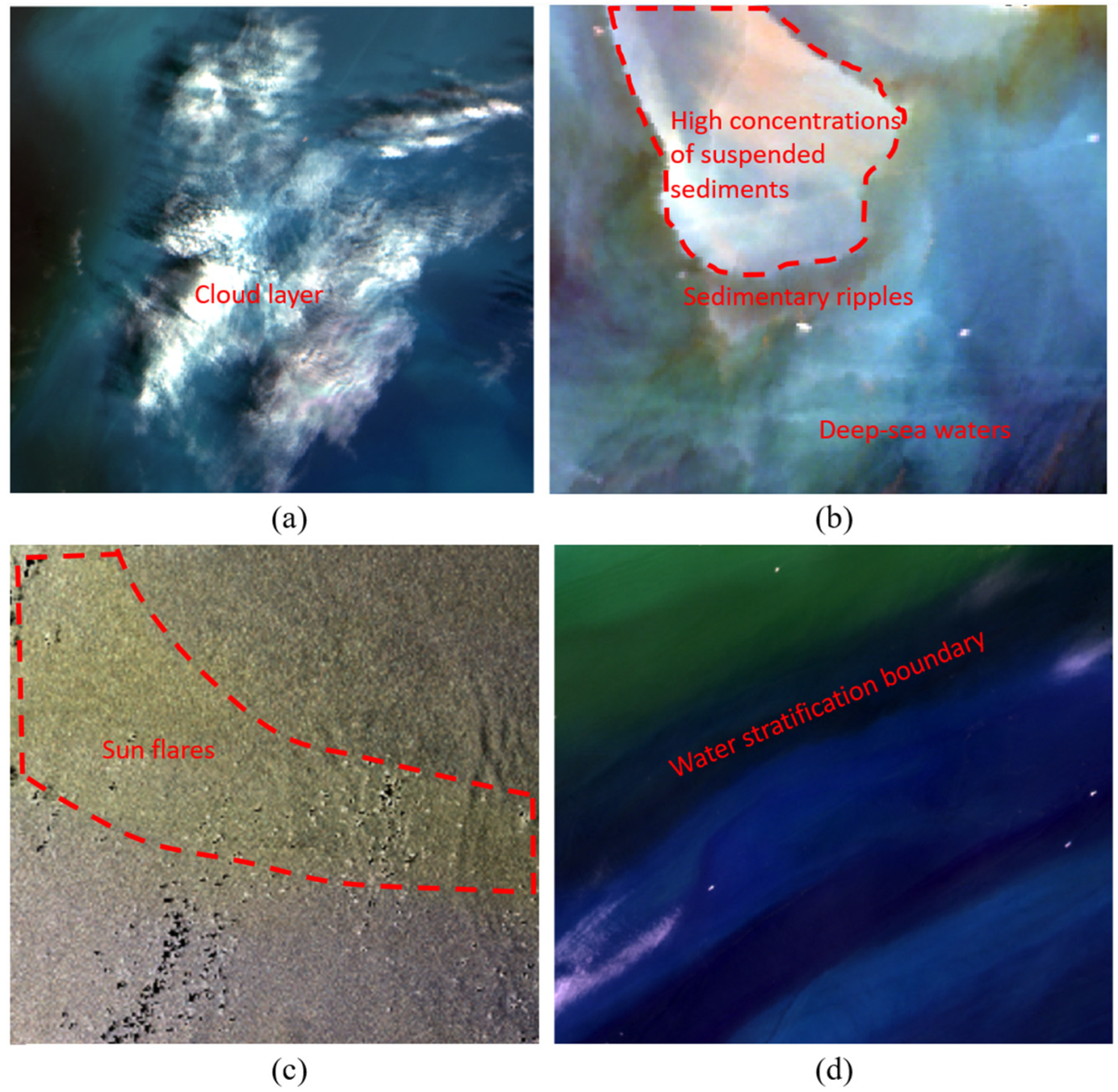
Selecting negative samples in a targeted manner constitutes an effective strategy for enhancing a classifier’s discriminative capability, having already been successfully applied in the domains of object detection and image segmentation [27]. In negative sample generation, the VB-FAH index is first calculated for the entire remote sensing image. Statistical analysis then identifies the VB-FAH index range [A, B] corresponding to annotated red tide areas. After threshold determination and extraction, this region represents non-red tide areas that are spectrally prone to confusion with red tides. The balance between positive and negative samples in a dataset influences the performance of subsequent model training [28]. Given that red tides occupy a relatively small proportion of the entire remote sensing image while ambiguous regions constitute a larger portion, negative samples are selected based on prior knowledge (Table S1). These primarily include: (a) cloud cover and cloud shadow areas; (b) coastal waters with high suspended sediment; (c) solar flare zones; (d) the transitional zone between pure deep seawater and shallow water. It contains 460 positive samples and 460 negative samples, clouds/shadows (25%), turbid water (25%), sun glint (25%), and shallow transition zones (25%). As illustrated in Figure 4, pixels within these regions were labeled as negative samples.

Data Augmentation

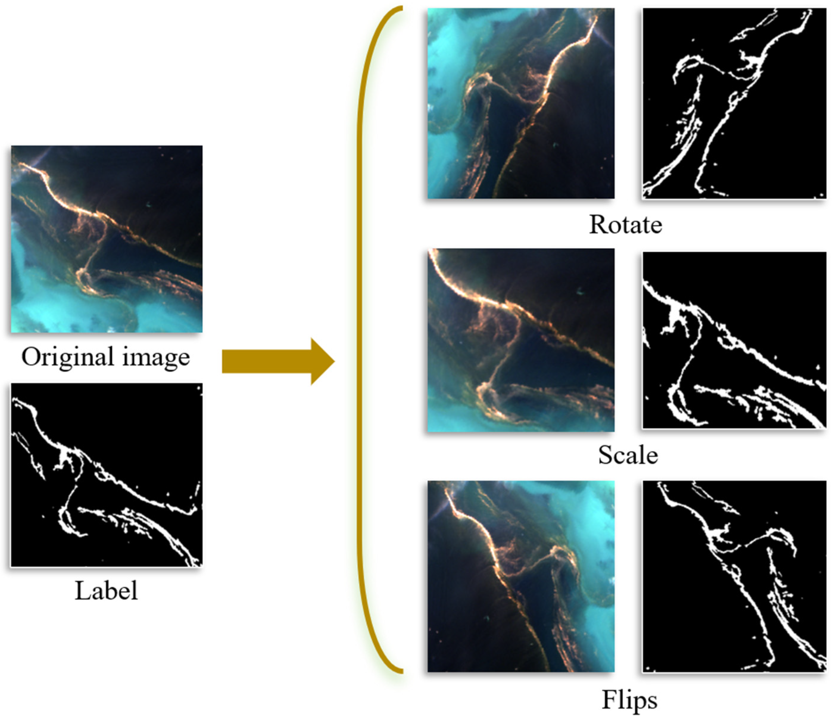
Data augmentation is a commonly employed technique to mitigate overfitting in deep learning models and enhance their generalization capabilities [29]. To increase data diversity and improve model generalization, training sample pairs (image patches and their corresponding label patches) undergo random horizontal/vertical flipping, 90-degree rotation, and brightness adjustments, as illustrated in Figure 5.

2.2.3. Model Architecture and Training

U-Net Model

The encoder employs the classical U-Net architecture, comprising four downsampling modules. Each module contains two 3 × 3 convolutional layers (followed by ReLU activation) and a 2 × 2 max-pooling layer, with the number of channels doubling at each stage [30]. The decoder corresponds to four upsampling modules, employing transposed convolutions for upsampling. These are concatenated with feature maps of the same scale as the encoder via skip connections, followed by two additional 3 × 3 convolutional layers. The final output layer utilizes 1 × 1 convolutions and a Sigmoid activation function to generate a probability map indicating the likelihood of each pixel being a red tide. Parameters: batch = 32, epochs = 100, early stopping patience.

Multi-Channel Input Design

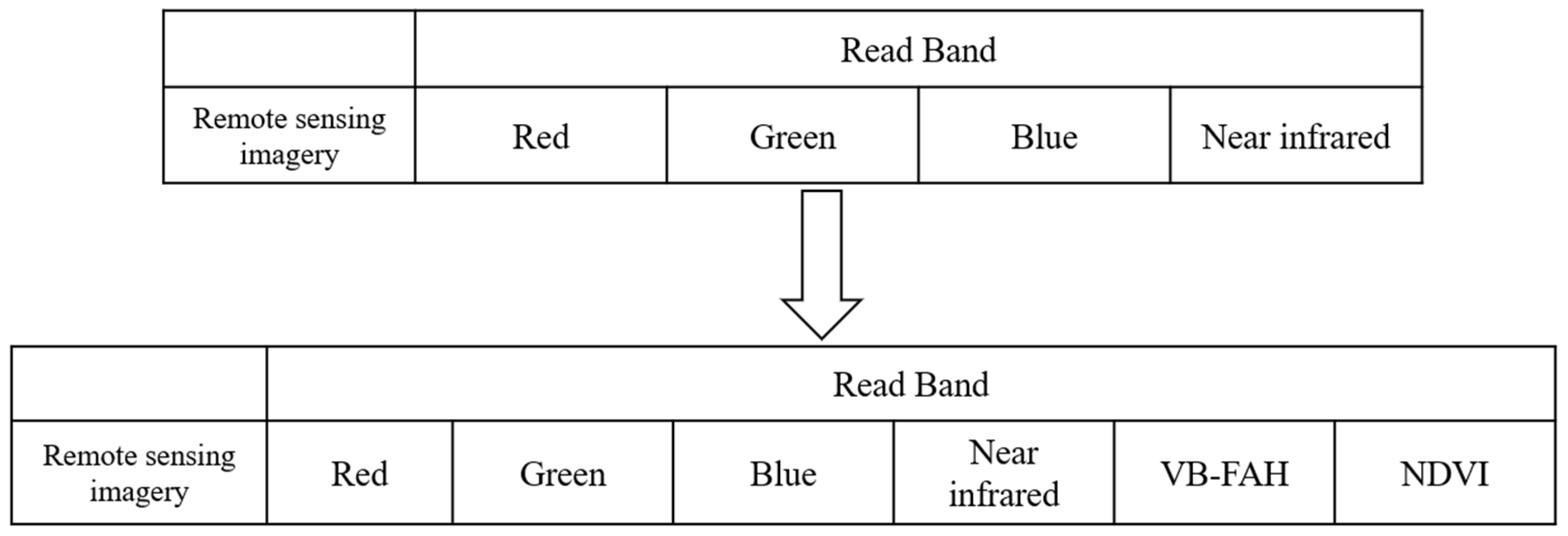
The model’s input comprises a four-channel tensor representing the satellite’s original blue, green, red, and near-infrared bands. Subsequent experiments also employed an approach of increasing the number of channels by adding a fifth and sixth channel, corresponding to pre-calculated NDVI and VB-FAH index data, respectively. A schematic diagram of the multi-channel design is shown in Figure 6. This design aims to provide the model with composite features that combine raw information with domain knowledge, enabling training that integrates these features with the labels.

2.2.4. Experimental Setup

The entire dataset was randomly partitioned into training, validation, and test sets in a 70%:15%:15% ratio. Experiments were conducted on a test rig equipped with an NVIDIA GeForce RTX 4060 Laptop GPU (Manufacturer: Tongfang Computer (Suzhou) Co., Ltd., located in Suzhou, Jiangsu Province, China; Country of purchase: China), with the overall implementation based on Python (3.10.8) and the TensorFlow framework. The model input size was 64 × 64 with four channels, producing a binary image of identical dimensions as output. Model training employed a composite loss function combining binary cross-entropy loss with Dice loss [31], utilizing the Adam optimizer with an initial learning rate of 0.001 and a learning rate decay strategy. The batch size was set to 16, with training conducted over 100 epochs. Training was terminated early when the validation set loss ceased to decrease, thereby preventing overfitting [32]. The validation set is used to real-time evaluate the generalization ability of the model during training and guide the early stopping strategy; the test set is independent of the training process and only used for the final validation of model performance.

To validate the effectiveness of each method, three sets of comparative experiments were designed:

• Experiment 1 (Targeted Sampling Method): Observe remote sensing imagery and, in conjunction with expert visual annotation, designate red tide areas as positive samples. Targeted negative samples were selected from areas extracted using the VB-FAH index, maintaining exact positive–negative sample ratio (1:1) containing 230 positive samples and 230 negative samples. The labels for both positive and negative sample areas, along with their corresponding four-band remote sensing imagery, were fed into the U-Net model for training. Subsequently, the remote sensing imagery requiring classification was input into the trained model, yielding a binary image indicating potential red tide occurrence (1 = potential occurrence, 0 = no potential occurrence).
• Experiment 2 (Random Negative Sampling Method): The positive sample creation, training, and subsequent recognition processes are identical to Experiment 1. Randomly generated negative samples are employed, maintaining a roughly equal number of positive and negative samples.
• Experiment 3 (Threshold Method): Calculate the VB-FAH index for the full-scene remote sensing image to obtain the index image. Locate the red tide outbreak area based on disaster bulletins, then visually adjust the index threshold until the red tide within the region is fully delineated. Segment the VB-FAH image within the threshold to obtain the extraction results.

2.2.5. Accuracy Assessment

Due to thin algal edges, cloud shadows, or shifts in annotations themselves, pixel-level IoU is highly sensitive to boundary misalignment. Consequently, relying on pixel-level precision metrics for overall identification results inevitably yields lower values. Furthermore, the complex sea conditions and meteorological factors within the study area significantly compromise the quality of remote sensing imagery. Event-level validation, however, focuses on the “alert or no alert” decision pertinent to public health. Following the NOAA Harmful Algal Bloom Event Reporting Standard [33], this study employs a method of comparing the spatial overlap between model-detected patches and the footprints of recorded events (GTEbox). Spatial overlap is defined as follows: If ∃ binary map polygon pi such that Overlap ≥ θ, then record as “detected”, TPevent = 1; otherwise record as “missed”, FNevent = 1; Defining image-level false positives: If the Overlap with any recorded event footprint GTEbox is <θ, and the set of binary polygons Pmod is non-empty, then FPevent = 1. After determining the detection status for each event, the following metrics are calculated for all N events: event-miss rate (EMR), false alarm rate (FAER), event-level overall accuracy (Accuracy), and F1 score. To visually represent false alarm recognition, this study additionally employs a method calculating the ratio of detected red tide area to total sea area. This is computed by dividing the area of red tide patches identified by each method by the sea area depicted in the remote sensing imagery, denoted as K. The calculation method is as follows.

$$\mathrm{O}\mathrm{v}\mathrm{e}\mathrm{r}\mathrm{l}\mathrm{a}\mathrm{p}(p_i,\mathrm{G}\mathrm{T}\mathrm{E})={\displaystyle \frac{\mathsf{\Sigma }\mathrm{T}\mathrm{P}\mathrm{e}\mathrm{v}\mathrm{e}\mathrm{n}\mathrm{t}\mathrm{A}\mathrm{r}\mathrm{e}\mathrm{a}(p_i\cap \mathrm{G}\mathrm{T}\mathrm{E}\mathrm{b}\mathrm{o}\mathrm{x})}{\mathrm{A}\mathrm{r}\mathrm{e}\mathrm{a}\left(\mathrm{G}\mathrm{T}\mathrm{E}\mathrm{b}\mathrm{o}\mathrm{x}\right)}}$$

(2)

$$EMR={\displaystyle \frac{\mathsf{\Sigma }\mathrm{N}\mathrm{P}\mathrm{e}\mathrm{v}\mathrm{e}\mathrm{n}\mathrm{t}}{\mathrm{N}}}$$

(3)

$$FAER={\displaystyle \frac{\mathsf{\Sigma }\mathrm{F}\mathrm{P}\mathrm{e}\mathrm{v}\mathrm{e}\mathrm{n}\mathrm{t}}{\mathrm{N}}}$$

(4)

$$\mathrm{Accuracy}=1-\mathrm{EMR}-\mathrm{FAER}$$

(5)

$$EventF1={\displaystyle \frac{2\times \left(1-\mathrm{E}\mathrm{M}\mathrm{R}\right)\times (1-\mathrm{F}\mathrm{A}\mathrm{E}\mathrm{R})}{(1-\mathrm{E}\mathrm{M}\mathrm{R})+(1-\mathrm{F}\mathrm{A}\mathrm{E}\mathrm{R})}}$$

(6)

$$Ki={\displaystyle \frac{S_{p_i}}{S_i}}$$

(7)

Pmod = {p_i, p_j, …, p_k}, N denotes the number of events, and S_i represents the area of the identified binary polygon.

To further validate the recognition performance, this study also conducted a spatio-temporal transfer experiment by selecting the HY-1D imagery from 13 April 2022, which featured relatively high image quality and visible red tide patches, and incorporating it into the aforementioned trained model for transfer recognition. The recognition effectiveness in the waters near Wenzhou was then observed.

3. Results

3.1. Experimental Results

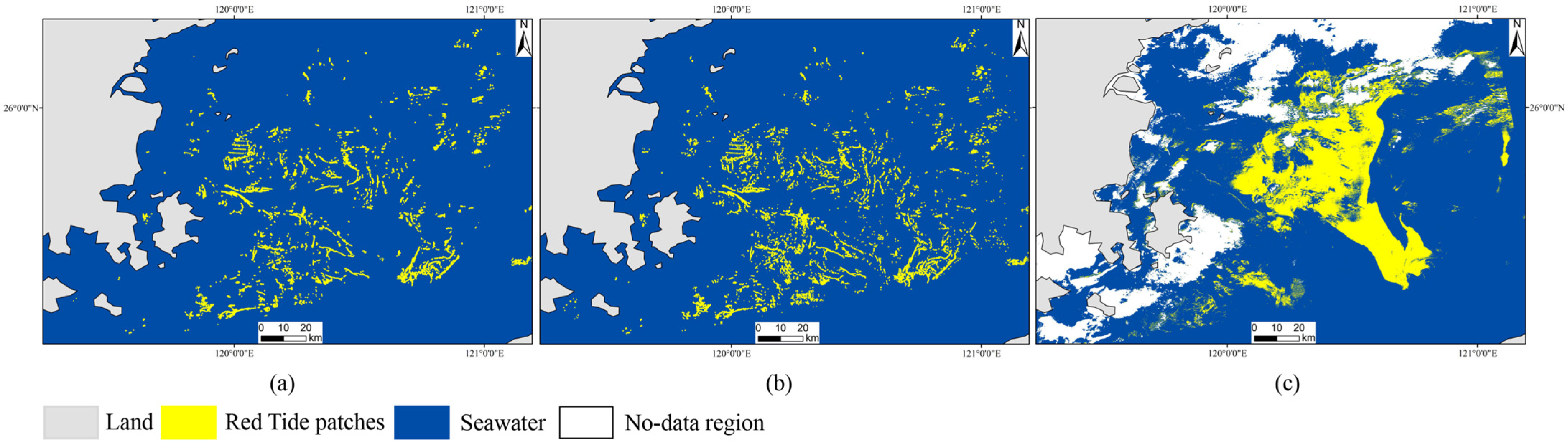
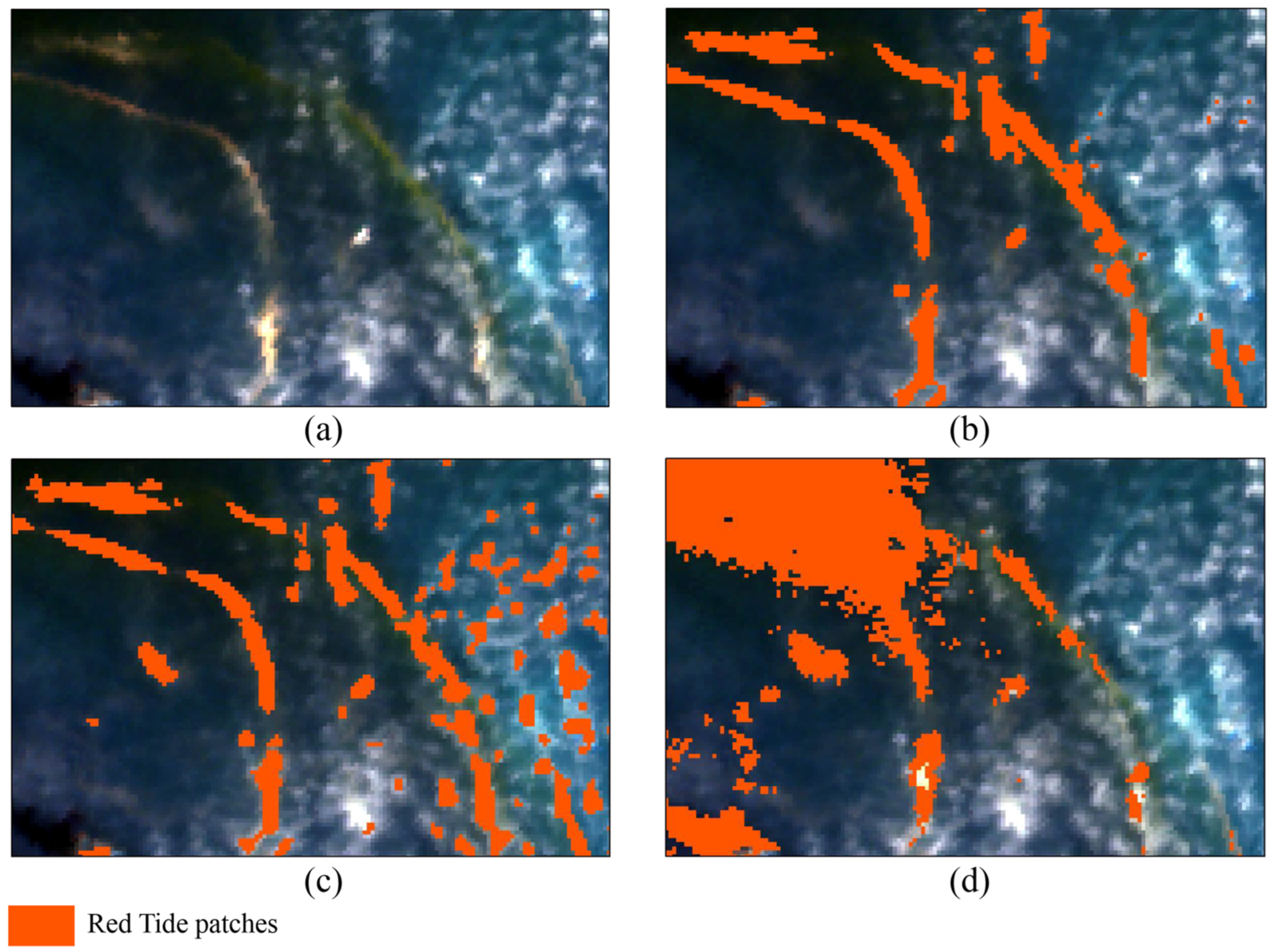
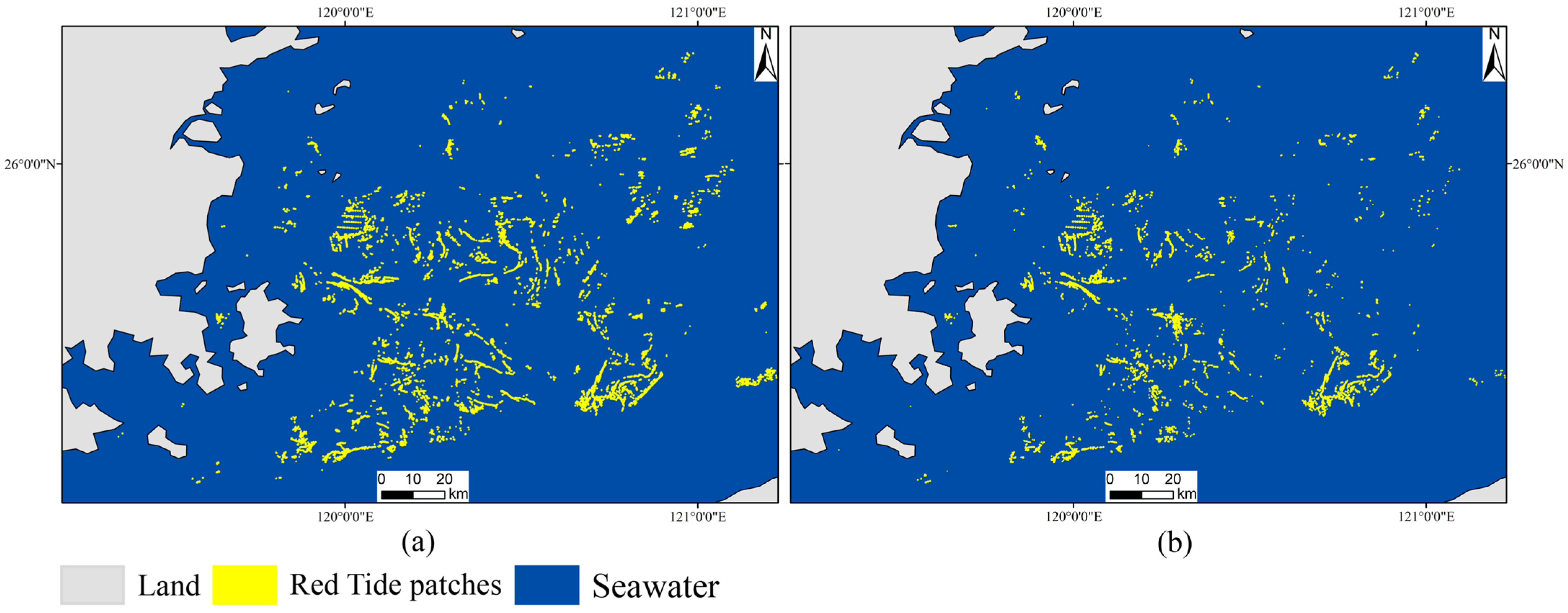
Figure 7a–c presents the experimental results for Experiments 1–3 and details of local red tide identification outcomes. Experiment 1 results are shown in Figure 7a. Inputting the entire remote sensing image enabled accurate identification of red tide patch locations with minimal false positives and effective avoidance of ambiguous regions. Figure 7b presents Experiment 2 results, where identified patches appeared more complex compared to Experiment 1, with misclassifications occurring in areas such as cloud cover, sun glare, sediment, and water boundary lines. Experiment 3 results are shown in Figure 7c. Adjusting thresholds enabled recognition of approximate red tide shapes, though large areas of water with differing brightness were misclassified. For enhanced observation, Figure 8a–d respectively present localized remote sensing imagery of key outbreak zones alongside identification details using the targeted sampling method, random sampling method, and thresholding method.

Table 3. Comparison of recognition accuracy across different methods (the total number of red tide event N = 11).

Method	IoU	PA	EMR (%)	FAER (%)	Accuracy (%)	EventF1 (%)	K
Targeted sample selection	0.6064	0.9291	9.09	9.09	81.82	90.91	0.0105
Random negative samples	0.6217	0.9365	9.09	18.18	72.73	86.12	0.0127
Threshold extraction	0.3582	0.6223	36.36	45.45	18.18	58.74	0.1631

summarizes the accuracy of red tide identification across different methods. Compared to threshold extraction and random sample selection, the targeted sample selection strategy reduces both the false negative rate and false positive rate while improving precision and F1 score.

3.2. Experimental Analysis

The comparative experiments designed in this study aimed to observe the effectiveness of the contrast threshold extraction method and the negative sample selection strategy. The recognition results of Experiment 1 are shown in Figure 7a, where it can be observed that inputting the entire remote sensing image directly outputs the red tide patch recognition results. The false negative rate of 9.09% indicates minimal missed detections, while the false positive rate of 9.09% suggests only a few instances of misclassification. Overall event-level precision reached 81.81%, with an event-level F1 score of 90.91%—representing improvements of 9.09% and 4.19% respectively over Experiment 2. The K-value was 0.0105. Analysis reveals that introducing targeted samples during dataset construction compelled the model to prioritize training on borderline regions prone to misclassification, thereby optimizing decision boundaries. Simultaneously, selectively employing ambiguous areas as negative samples prevented the model from “learning” these as algal blooms. Consequently, the identified potential outbreak zones more closely align with actual algal bloom patch extents. Comparing recognition results in Figure 8b,c, the targeted negative sample selection strategy demonstrably mitigates the influence of confusing regions, directly contributing to the significant reduction in false detection rates. Contrasting Figure 8b,d indicates this method prevents large-scale misclassifications. Analysis reveals that the U-Net model constructs an intrinsic representation of the complex spatio–spectral features of red tides by learning from extensive samples. This representation offers greater discriminative power and robustness than a single index threshold, enabling adaptation to image variations under diverse environmental conditions. It not only eliminates the need for repeated threshold adjustments but also facilitates direct recognition of entire images, significantly enhancing extraction efficiency and accuracy, thus enabling global red tide identification. Given the poor quality of currently available imagery and the highly complex marine environment, using remote sensing data inevitably introduces some false positives. However, for regions where red tide outbreaks are confirmed, false negatives are virtually absent. Experimental results align with practical conditions, and the overall accuracy meets real-world application requirements.

Figure 7b of Experiment 2’s recognition results indicates that the model can identify the approximate locations of blooms. However, it also misidentifies certain easily confused areas—such as coastal sediment, water bodies with brightness similar to red tides, cloud cover, and solar flares—as red tides. The false negative rate stands at 9.09%, while the false positive rate is 18.18%, demonstrating reduced instances of both missed detections and misclassifications. The overall event-level accuracy reached 72.73%, with an event-level F1 score of 86.12%. Compared to the threshold extraction method, this represents improvements of 54.55% and 27.38%, respectively. The observed K value of 0.0127 aligns with the actual proportion of red tide coverage within the total sea area. Comparing Figure 8b,c reveals that the random sampling method exhibits higher false detection rates. Analysis indicates that during initial positive sample labeling, not only grid cells containing red tides were utilized, but also background waters adjacent to red tides. This effectively ‘taught’ the model to identify red tide patches against newly defined background areas, thereby avoiding large-scale false positives and false negatives. However, negative samples in this experiment were randomly selected and may not have included areas prone to confusion, naturally leaving the model unable to prevent certain misclassifications. Overall, compared to threshold extraction, this method achieves greater automation and more precise identification, albeit with a slight reduction in accuracy.

The results of the threshold extraction method in Experiment 3 are shown in Figure 7c. While extraction within small-scale red tide outbreak areas (within a uniform brightness zone) yielded satisfactory results, large swathes of the broader area were potentially misidentified as red tide. The event-level false negative rate of 36.36% was relatively high. Analysis revealed that in certain water bodies with overall low brightness, all red tide patches within them went undetected. The false alarm rate of 45.45% is also elevated. Observing the K value of 0.1631 indicates that detected red tide patches occupied 16.31% of the total sea area, far exceeding actual coverage. Figure 8d demonstrates that the threshold method produces extensive false positives, misclassifying several ambiguous regions as potential red tide occurrences, thereby inflating the false alarm rate. Although this method can rapidly extract the approximate shape of red tides, prior knowledge of their appearance is required as background information for accurate classification. Furthermore, complex sea conditions (cloud cover, sun glare, water body reflection colors, etc.) cause significant brightness variations across different regions of the remote sensing imagery, leading to substantial discrepancies in calculated indices. Consequently, different thresholds are required for extracting distinct small regions. When applied to an entire HY-1D satellite image (approximately 2900 km wide), selecting a single threshold for extraction proves challenging. Achieving precise extraction for each segment would necessitate adjusting thresholds based on image brightness, manually avoiding areas prone to interference, cropping small regions for threshold extraction, and subsequently stitching them together to achieve global recognition. This approach is impractical for real-world applications.

3.3. Multi-Channel Comparison

To further enhance recognition accuracy, Experiment 4 was conducted by incorporating NDVI and VB-FAH as additional input channels, resulting in a six-channel input model. As shown in Figure 9 and

Table 4. Multi-channel experimental accuracy comparison.

Method	IoU	PA	EMR (%)	FAER (%)	Accuracy (%)	EventF1 (%)	K
Targeted sample selection	0.6064	0.9291	9.09	9.09	81.82	90.91	0.0105
Six-channel training	0.5692	0.9416	18.18	9.09	72.73	86.12	0.0062

, compared to Experiment 3, the model identified narrower red tide patches with smaller areas. Some recognized patches failed to fully cover the actual red tide patches. Calculating the K value indicates that the identified red tide patches covered only 0.62% of the total sea area. Furthermore, within confirmed red tide occurrence zones, partial missed detection occurred, yielding a missed detection rate of 18.18%, signifying that a portion of red tides remained undetected. Analysis indicates that NDVI and VB-FAH are discriminative enhancement features constructed from original spectral bands, which highlight the spectral differences between targets and interferences and help the model quickly focus on key regions, without providing additional independent observation information. However, NDVI and VB-FAH exhibit strong information redundancy with the original spectral channels. These indices rely on fixed band combinations and computational forms, which tend to guide the model toward local features highly correlated with the labels (VB-FAH). Such feature self-verification leads to good performance in the training area but increases the overfitting risk and reduces generalization ability in unseen regions.

3.4. Migration Identification and Verification

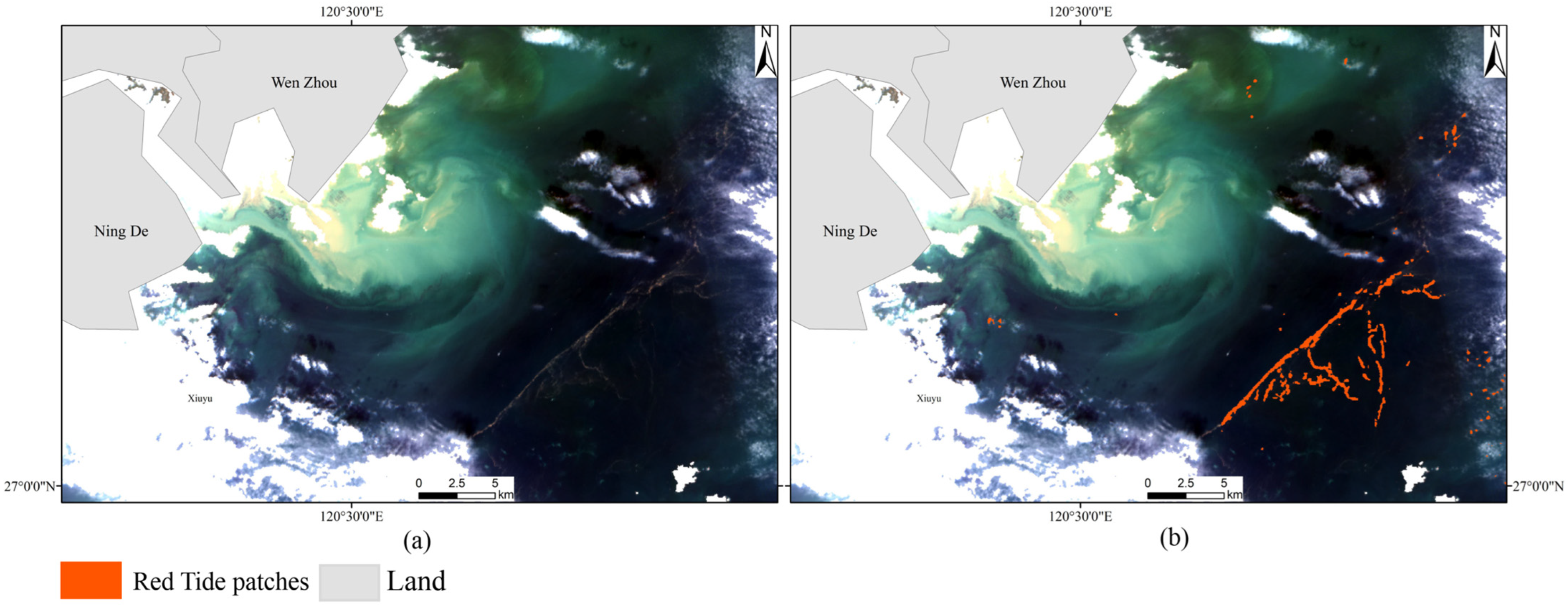
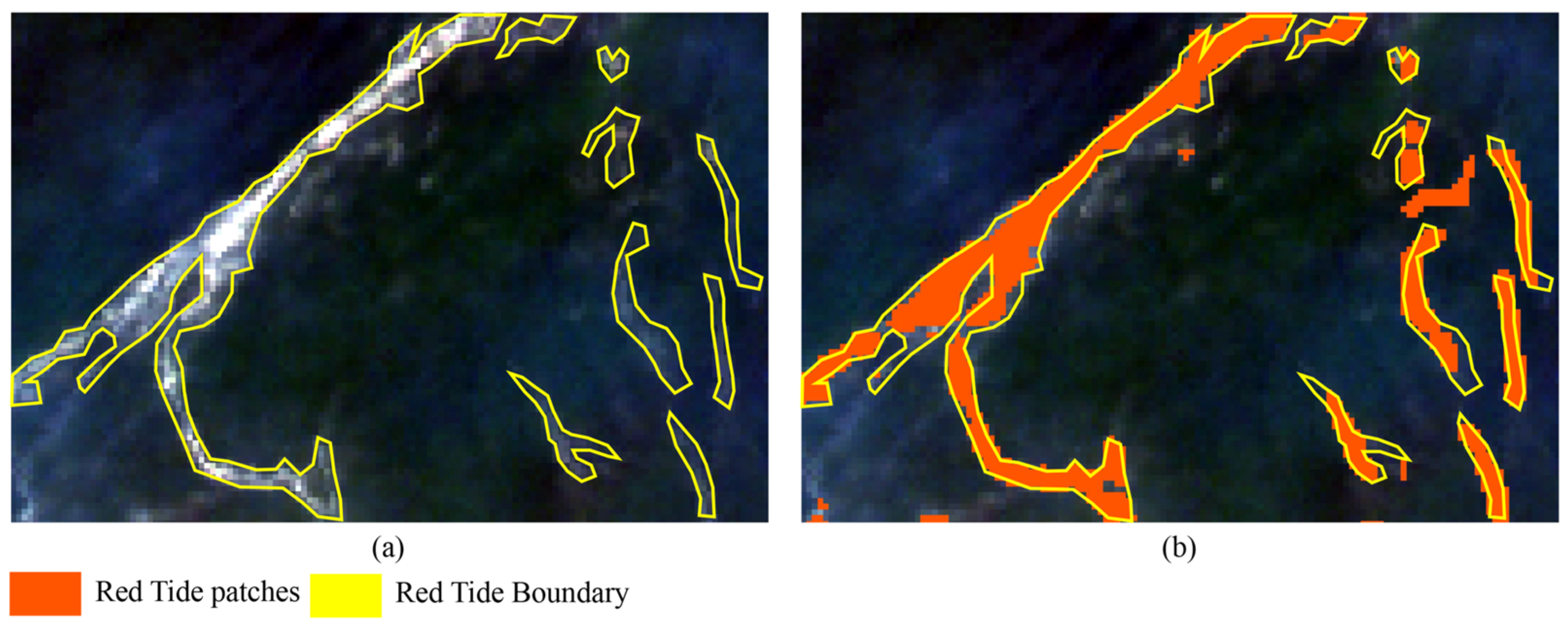
Remote sensing imagery of the waters near Wenzhou on 13 April 2022 is shown in Figure 10a. The identification results obtained by applying the model trained using the aforementioned deep learning approach (targeted sample method) are presented in Figure 10b, Figure 11a,b show the detailed enlarged views of the remote sensing image and the recognition results for transfer learning identification. The experimental results demonstrate that the model can accurately identify red tide patches with precise positioning and clear zonal distribution. It effectively circumvents the influence of cloud cover and sediment, proving that transfer learning achieves satisfactory recognition performance across different spatiotemporal imagery. This outcome aligns with practical application requirements.

4. Discussion

4.1. Measurement of Efficiency Gains in Targeted Sampling Strategies

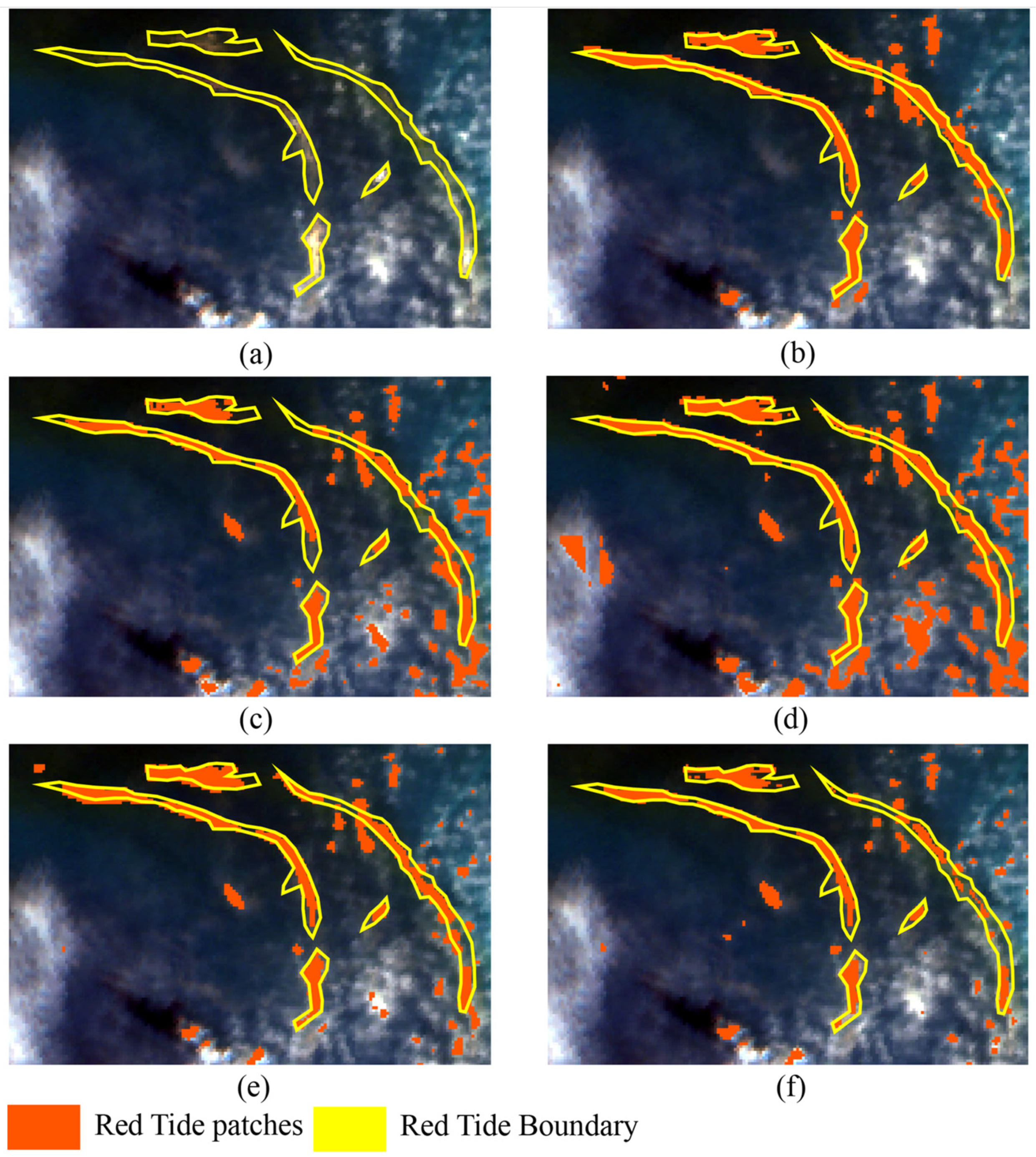
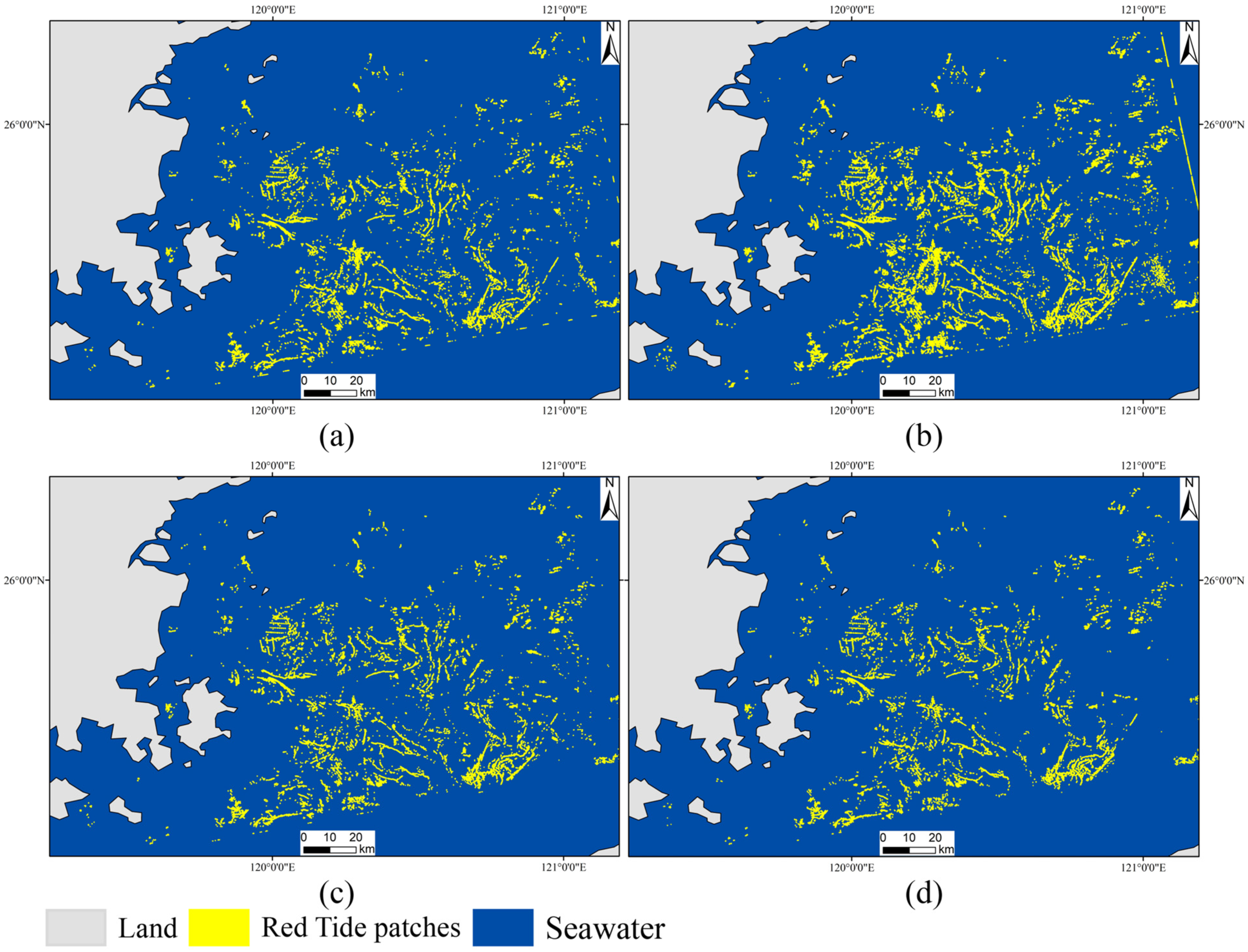
Sample selection is pivotal to enhancing experimental efficiency. Selecting negative samples in a targeted manner can reduce the workload involved in sample selection and improve the efficiency of the experiment. Chen Yaxin [34] employed seven hybrid sampling strategies in classification experiments within her research on hyperspectral image classification methods based on attention mechanisms and active learning, demonstrating that active learning sampling approaches can enhance sample selection efficiency. Zhang Yurong [35] integrated self-supervision with active learning into a unified framework in her study on active learning-based polarimetric SAR image classification, thereby improving the efficiency of manual annotation. To measure the efficiency gains of targeted sample selection strategies, Experiment 5 was designed with a four-channel input model using random negative samples. Unlike Experiment 2, this experiment increased the number of negative samples. To control variables, negative samples were set at 2×, 4×, 8×, and 16× quantities to observe the threshold at which targeted sample selection achieves training effectiveness. The overall recognition results are presented in Figure 12a–d. For enhanced observation, Figure 13c–f displays localized recognition outcomes for each experiment. Figure 13a–f, respectively, shows the corresponding remote sensing imagery and recognition results using the targeted sample method. Results indicate that as the number of random negative samples increases to four times the target sample size, the identified red tide patches become more chaotic and densely clustered, with broader and larger red tide bands. False alarms occur in complex water bodies, cloud cover, and sediment areas. When negative samples reached eight times the targeted sample size, accuracy approached parity with largely equivalent recognition outcomes. Further increasing negative samples to sixteen times yielded essentially unchanged identified red tide patches, indicating a stabilizing trend. Analysis indicates that increasing random negative samples enhances coverage of ambiguous regions but may also include areas that should be classified as positive samples. This introduces bias during model training, leading to missed detections or false positives. Comparative experiments demonstrate that achieving equivalent recognition accuracy requires expanding random negative samples to at least eight times the number of positive samples. Consequently, the targeted negative sample selection method employed in this study requires substantially fewer samples than random sampling—only 1/8 of the negative samples required for random sampling—yielding an 87.5% efficiency gain. From an application perspective, this strategy proves markedly superior.

4.2. The Advantages and Necessity of Incorporating Remote Sensing Interpretation into Red Tide Monitoring

The two primary methods for interpreting red tides are probabilistic modeling based on mechanistic models and in situ observation via field stations, each possessing distinct advantages and limitations. Model-based approaches typically involve calculating physical, chemical, and various biological parameters to derive predictions [36]. In his study on diatom red tide early warning models for aquaculture zones in the Pingtan Sea Area [37], Zou Jiashu integrated data on chlorophyll a, dissolved oxygen, apparent oxygenation, air temperature, precipitation, and wind speed. He calculated Pearson correlation coefficients and conducted correlation analyses to establish a foundation for constructing a BP (Back Propagation) neural network model. The approach of using mechanistic models to predict red tide occurrence probabilities possesses a priori advantages. It can provide probability levels for future red tide events and enable grid-based forecasting across entire bays or even provincial marine areas. This method offers low marginal costs and extensive spatial coverage. However, it requires substantial quantities of continuous, high-quality, and multi-source historical data to train effective models. Furthermore, overfitting is prone to occur in different regions, leading to missed detections or false positives. Should the model be applied to a different marine area, retraining and transfer learning become necessary.

The most traditional monitoring method involves establishing field stations for in situ observation, namely manual on-site observation or sampling aboard vessels [1]. Planktonic algae are concentrated using filter nets, fixed with preservatives, and transported to laboratories for manual counting under microscopes using phytoplankton counting frames to monitor red tides [38]. The primary data for routine and emergency monitoring of red tides are biological parameters, specifically the analysis and counting of red tide algal species and abundance. The individual counting method is commonly employed, providing reliable detection of species present in water samples while also enabling accurate assessment of cell abundance. Among various novel monitoring methodologies, manual counting remains the most reliable and direct reference method across research and surveys. However, its sample preparation is cumbersome and time-consuming, requiring operators to possess advanced expertise in plankton and identification experience. These labor-intensive demands limit the spatial coverage and timeliness of this measurement approach. In situ observation methods, not reliant on historical data, enable direct data acquisition through instrumentation. They offer high real-time capability and provide accurate information on dominant algal species and cell abundance. However, sample preparation is challenging, and data collection is typically limited to single points and time points. This approach suffers from temporal lag and limited spatial coverage. Achieving large-scale monitoring would necessitate increasing the number of stations, entailing high and difficult construction and maintenance costs.

The advent of remote sensing monitoring methods has resolved many of the aforementioned challenges. In recent years, an increasing number of models and algorithms employing remote sensing techniques have been developed for studying red tides, including single-band models, dual-band difference or ratio models, multi-band difference-ratio models, numerical simulations, neural networks, and genetic algorithms [39]. Although remote sensing imagery is constrained by revisit periods and resolution limitations, the spatio-temporal resolution of the HY-1D satellite data utilized in this study is sufficient to support red tide research. Furthermore, remote sensing monitoring offers extensive spatial coverage, low observation costs, and ease of data acquisition. In red tide research, it compensates for the limitations of traditional methods, playing an irreplaceable role. By integrating remote sensing interpretation into a three-dimensional red tide monitoring system, this study reduced false negative rates by 27% and false positive rates by 36% compared to threshold-based methods alone, with an overall F1 score improvement of 0.3217. This approach addresses the limitations of traditional mechanistic modeling and field station measurements; for highly dynamic red tide events where in situ observation is challenging, it enables relatively accurate identification and monitoring, along with spatio-temporal transfer recognition, thereby meeting practical application requirements.

4.3. Limitations and Future Development

Compared to mainstream research employing deep learning for red tide detection, this study innovates by introducing a targeted negative sample selection strategy. This approach systematically reduces the false positive rate in red tide detection—a practical application challenge—while simultaneously enhancing the efficiency of sample selection. At the application level, this research not only provides a model but also delivers a comprehensive solution workflow encompassing negative sample construction and feature engineering.

However, this study still has certain limitations: Firstly, the model’s performance relies heavily on the quality of training samples. Currently, the use of remote sensing imagery to study complex oceans presents various difficulties, and its recognition capability may diminish for specific types of red tides or under environmental conditions with anomalous spectral reflectance, such as Noctiluca scintillans blooms (which exhibit distinct backscattering due to gas vacuoles) compared to Karenia mikimotoi (strong chlorophyll absorption features). Secondly, computational requirements on the RTX 4060 Laptop GPU (2.3 TFLOPS peak, 8 GB VRAM) currently limit real-time processing to 0.8 scenes/minute, the U-Net model has a large number of parameters, and its computational efficiency requires further optimization for large-scale, real-time operational deployment. Thirdly, limited by the spectral characteristics of remote sensing images, it is difficult for us to quantitatively define red tide targets. The method used in this study does not detect the true red tide extent but rather identifies regions with high biomass accumulation determined by visual spectral characteristics.

Looking ahead, research efforts may proceed along the following lines: Firstly, constructing and open-sourcing a larger-scale, multi-source, high-quality standard red tide remote sensing detection dataset to advance the field; secondly, exploring lightweight network architectures to enhance inference speed while maintaining accuracy; thirdly, migrating this framework for application to monitoring other types of algal blooms or marine phenomena to test its universality.

5. Conclusions

This paper successfully establishes a practical workflow for red tide detection, standardizes data screening methodologies, and develops an automated remote sensing framework for red tide identification. This framework employs a U-Net deep learning architecture, integrating targeted sample selection strategies with multispectral feature inputs. By incorporating remote sensing techniques into a three-dimensional red tide monitoring system, the proposed framework achieves a 27% reduction in false negatives and a 36% decrease in false positives compared to traditional threshold-based extraction methods. The overall F1 score improved by 0.3217. Compared to deep learning methods using simple random samples, false alarm rates decreased by 9.09%, the F1 score increased by 0.0479, and sample selection efficiency rose by 87.5%. This approach effectively addresses the core issues of traditional threshold-based methods: high false negative rates, low automation, poor adaptability, and vulnerability to interference. Through an innovative training sample construction approach, the model achieves red tide patch identification with low misclassification and false alarm rates. Crucially, it requires no manual parameter adjustments for each new image scene. When confronted with novel remote sensing imagery across varying spatio-temporal contexts, the model delivers rapid and accurate identification, meeting practical application demands. Experiments demonstrate the method’s outstanding robustness in complex scenarios, providing a robust and reliable technical pathway towards operationalizing intelligent red tide remote sensing identification.

References

1. Lee, M.-S.; Arrigo, K.; Smith, A.; Woodson, C.B.; Lee, J.; Micheli, F. Monitoring Harmful Algal Blooms in the Southern California Current Using Satellite Ocean Color and In Situ Data. J. Mar. Sci. Eng. 2025, 13, 2044. [Google Scholar] [CrossRef]
2. Li, J.; Xing, Q.; Zheng, X.; Li, L.; Wang, L. A Method for Extracting Noctiluca scintillans Red Tide from UAV Images Based on Deep Learning. J. Comput. Appl. 2022, 42, 2969–2974. [Google Scholar]
3. Xu, Y. Research on Red Tide Drift and Diffusion in Lingdingyang Based on Satellite Remote Sensing and Numerical Simulation Methods. Master’s Thesis, Guangdong Ocean University, Zhanjiang, China, 2023. [Google Scholar]
4. Zuo, S.; Li, B. Marine Disasters Characteristics and Its Prevention Measures in China over the Past 20 Years. Meteorol. Disaster Reduct. Res. 2008, 31, 28–33. [Google Scholar]
5. Tu, C. Hazard Assessment of Red Tide in Zhanjiang Offshore Based on Long Time Series Sentinel-2 Images. Resour. Guide 2025, 10, 22–25. [Google Scholar]
6. Sakuno, Y.; Maeda, A.; Mori, A.; Ono, S.; Ito, A. A Simple Red Tide Monitoring Method using Sentinel-2 Data for Sustainable Management of Brackish Lake Koyama-ike, Japan. Water 2019, 11, 1044. [Google Scholar] [CrossRef]
7. Wang, R. Extraction of Red Tide Information in the East China Sea Based on GOCI Remote Sensing Data. Master’s Thesis, Shanghai Ocean University, Shanghai, China, 2018. [Google Scholar]
8. Liu, R.-J.; Zhang, J.; Cui, B.-G.; Ma, Y.; Song, P.-J.; An, J.-B. Red Tide Detection Based on High Spatial Resolution Broad Band Satellite Data: A Case Study of GF-1. J. Coast. Res. 2019, 90, 120–128. [Google Scholar] [CrossRef]
9. Jiang, D.; Zhang, H. Spatio-Temporal Characteristics Analysis of Chlorophyll-a Concentration in the Bohai Sea and Its Application in Red Tide Monitoring. Mar. Sci. 2018, 42, 23–31. [Google Scholar]
10. Lee, M.-S.; Park, K.-A.; Micheli, F. Derivation of Red Tide Index and Density Using Geostationary Ocean Color Imager (GOCI) Data. Remote Sens. 2021, 13, 298. [Google Scholar] [CrossRef]
11. Hu, C. A novel ocean color index to detect floating algae in the global oceans. Remote Sens. Environ. 2009, 113, 2118–2129. [Google Scholar] [CrossRef]
12. Feng, Z.; Yang, X.; Sun, X.; Du, Z.; Liu, R. Developing Process Detection of Red Tide Based on Multi-Temporal GOCI Images. In Proceedings of the 2018 10th IAPR Workshop on Pattern Recognition in Remote Sensing (PRRS), Beijing, China, 19–20 August 2018. [Google Scholar]
13. Hill, P.R.; Kumar, A.; Temimi, M.; Bull, D.R. HABNet: Machine Learning, Remote Sensing-Based Detection of Harmful Algal Blooms. IEEE J. Sel. Top. Appl. Earth Obs. Remote Sens. 2020, 13, 3229–3239. [Google Scholar] [CrossRef]
14. Zhu, X.X.; Tuia, D.; Mou, L.; Xia, G.; Zhang, L.; Xu, F.; Fraundorfer, F. Deep Learning in Remote Sensing: A Comprehensive Review and List of Resources. IEEE Geosci. Remote Sens. Mag. 2017, 5, 8–36. [Google Scholar] [CrossRef]
15. Ronneberger, O.; Fischer, P.; Brox, T. U-Net: Convolutional Networks for Biomedical Image Segmentation. In Proceedings of the Medical Image Computing and Computer-Assisted Intervention (MICCAI), Munich, Germany, 5–9 October 2015; pp. 234–241. [Google Scholar]
16. Han, Y.; Ding, T.; Cui, P.; Wang, X.; Zheng, B.; Shen, X.; Ma, Z.; Zhang, Y.; Pan, H.; Yang, S. Red Tide Detection Method Based on Improved U-Net Model-Taking GOCI Data in East China Sea as an Example. Sensors 2023, 23, 9195. [Google Scholar] [CrossRef] [PubMed]
17. Kim, S.M.; Shin, J.; Baek, S.; Ryu, J. U-Net Convolutional Neural Network Model for Deep Red Tide Learning Using GOCI. J. Coast. Res. 2019, 90, 302–309. [Google Scholar] [CrossRef]
18. Li, J. Research on Extraction Algorithms for Green Tide and Red Tide Based on Machine Learning. Master’s Thesis, Ludong University, Yantai, China, 2022. [Google Scholar]
19. Long, J.; Shelhamer, E.; Darrell, T. Fully Convolutional Networks for Semantic Segmentation. IEEE Trans. Pattern Anal. Mach. Intell. 2015, 39, 640–651. [Google Scholar]
20. Liu, Y.; Kong, F.; Yu, R.; Chu, Y. Detection of Gonyaulax polygramma Based on FlowCam Images and YOLOv3 Deep Learning Model. Mar. Sci. 2024, 48, 15–23. [Google Scholar]
21. Badrinarayanan, V.; Kendall, A.; Cipolla, R. SegNet: A Deep Convolutional Encoder-Decoder Architecture for Image Segmentation. IEEE Trans. Pattern Anal. Mach. Intell. 2017, 39, 2481–2495. [Google Scholar] [CrossRef]
22. Ministry of Natural Resources of People’s Republic of China. China Marine Disaster Bulletin 2022 [EB/OL]. Available online: http://gi.mnr.gov.cn/202304/t20230412_2781112.html (accessed on 17 April 2025).
23. Liu, Y.; Zhang, Y.; Yao, H.; Zheng, Z.; Zhao, W.; Lin, G. Analysis on Bacterial Community of Noctiluca scintillans Algal Blooms Near Pingtan Island, China. Biology 2025, 14, 101. [Google Scholar] [CrossRef]
24. Zhao, X.; Liu, R.; Ma, Y.; Xiao, Y.; Ding, J.; Liu, J.; Wang, Q. Red Tide Detection Method for HY−1D Coastal Zone Imager Based on U−Net Convolutional Neural Network. Remote Sens. 2022, 14, 88. [Google Scholar] [CrossRef]
25. Sun, K.; Jiang, G.; Wang, N.; Yu, D.; Teng, J.; Gao, S.; Huang, J.; Zhao, Z.; Song, Y.; Xin, L.; et al. A semantic segmentation network for red tide detection based on enhanced spectral information using HY-1C/D CZI satellite data. Mar. Pollut. Bull. 2025, 215, 117813. [Google Scholar] [CrossRef]
26. Shi, F.; Liu, M.; Zhou, W. Study on radiation atmospheric correction method for second class water body using SeaWiFS data. J. Inn. Mong. Norm. Univ. 2006, 78, 424–427+432. [Google Scholar]
27. Wang, Q.; Wu, B.; Zhu, P.; Li, P.; Zuo, W.; Hu, Q. ECA-Net: Efficient Channel Attention for Deep Convolutional Neural Networks. In Proceedings of the 2020 IEEE/CVF Conference on Computer Vision and Pattern Recognition (CVPR), Seattle, WA, USA, 14–19 June 2020. [Google Scholar]
28. Chen, X. Research on Extraction Method of Rice Production Facility Land from Remote Sensing Images Based on Deep Learning. Master’s Thesis, Northeast Agricultural University, Harbin, China, 2025. [Google Scholar]
29. Shorten, C.; Khoshgoftaar, T.M. A survey on Image Data Augmentation for Deep Learning. J. Big Data 2019, 6, 60. [Google Scholar] [CrossRef]
30. Huang, Y. Research on Low-Altitude Remote Sensing Identification and Sample Migration of Crops in Complex Scenes in Karst Mountainous Areas. Master’s Thesis, Guizhou Normal University, Guiyang, China, 2024. [Google Scholar]
31. Sudre, C.H.; Li, W.; Vercauteren, T.; Ourselin, S.; Cardoso, M.J. Generalised Dice overlap as a deep learning loss function for highly unbalanced segmentations. In Proceedings of the Deep Learning in Medical Image Analysis and Multimodal Learning for Clinical Decision Support, Quebec City, QC, Canada, 14 September 2017; pp. 240–248. [Google Scholar]
32. Prechelt, L. Early Stopping—But When? In Neural Networks: Tricks of the Trade; Springer: Berlin/Heidelberg, Germany, 1998; pp. 55–69. [Google Scholar]
33. Stumpf, R.P.; Tomlinson, M.C. Remote sensing of harmful algal blooms. In Remote Sensing of Coastal Aquatic Environments; Springer: Dordrecht, The Netherlands, 2005; pp. 277–296. [Google Scholar]
34. Chen, Y. Research on Hyperspectral Image Classification Method Based on Attention Mechanism and Active Learning. Master’s Thesis, Wuhan University of Technology, Wuhan, China, 2021. [Google Scholar]
35. Zhang, Y. Research on Polarimetric SAR Image Classification Method Based on Active Learning. Master’s Thesis, Xi’an University of Posts & Telecommunications, Xi’an, China, 2024. [Google Scholar]
36. Xu, Y. Research on Red Tide Warning in Pingtan Sea Area, Fujian Province. Master’s Thesis, Fujian Normal University, Fuzhou, China, 2020. [Google Scholar]
37. Zou, J. Research on Early Warning Model for Dinoflagellate Red Tide in Aquaculture Area of Pingtan Sea. Master’s Thesis, Fujian Normal University, Fuzhou, China, 2022. [Google Scholar]
38. Hao, Y. Research on a Red Tide Algae Concentration Monitoring Device Based on Automatic Image Counting. Master’s Thesis, Xiamen University, Xiamen, China, 2022. [Google Scholar]
39. Qin, M. Research on Remote Sensing Identification and Prediction Methods for Red Tide in Coastal Waters Based on Spectral Characteristics. Master’s Thesis, Dalian Maritime University, Dalian, China, 2024. [Google Scholar]
Figure 1. HY-1D CZI L2A level remote sensing imagery of the study area (Changle District and Pingtan County, Fuzhou) on 23 April 2022 (50 m spatial resolution).
Jmse 14 00556 g001
Figure 2. Remote Sensing Identification Process for Red Tide Based on Targeted Sample Selection Strategy. Blue (√) indicates successful selection, and red (×) indicates non-selection.
Jmse 14 00556 g002
Figure 3. Sample Preparation Diagram.
Jmse 14 00556 g003
Figure 4. (a) Cloud cover and shadowed areas (b) Nearshore water body with high suspended sediment content (c) Solar flare zone (d) Transition zone between pristine deep seawater and shallow water.
Jmse 14 00556 g004
Figure 5. Schematic Diagram of Data Augmentation.
Jmse 14 00556 g005
Figure 6. Schematic Diagram of Multi-Channel Input Design.
Jmse 14 00556 g006
Figure 7. Results of red tide identification using different methods (a) Experiment 1: Deep learning method (targeted negative samples) (b) Experiment 2: Deep learning method (random samples) (c) Experiment 3: Threshold extraction method.
Jmse 14 00556 g007
Figure 8. Demonstration of Local Recognition Performance (a) Local remote sensing imagery (b) Experimental result 1: Deep learning method (targeted samples) (c) Experimental result 2: Deep learning method (random samples) (d) Experimental result 3: Thresholding method.
Jmse 14 00556 g008
Figure 9. Results of red tide identification using different methods: (a) Experimental Method 3: Deep learning approach (with targeted negative sample selection) (b) Experimental Method 4: Six-band approach (with targeted negative sample selection).
Jmse 14 00556 g009
Figure 10. (a) Remote sensing imagery of the migration identification verification area (b) Migration identification verification results.
Jmse 14 00556 g010
Figure 11. Demonstration of Local Image Recognition in Migration: (a) Local remote sensing image (b) Local recognition results.
Jmse 14 00556 g011
Figure 12. Deep learning-based red tide detection results (with varying numbers of random negative samples) (a) Detection results with 2× random negative samples (b) Detection results with 4× random negative samples (c) Detection results with 8× random negative samples (d) Detection results with 16× random negative samples.
Jmse 14 00556 g012
Figure 13. Deep learning method (with varying numbers of random negative samples) for localized red tide detection results: (a) Localized remote sensing imagery and actual red tide boundary (b) Localized red tide detection results using deep learning (with targeted negative samples) (c) Localized red tide detection results with 2× random negative samples (d) Localized red tide detection results with 4× random negative samples (e) Localized red tide detection results with 8× random negative samples (f) Localized red tide detection results with 16× random negative samples.
Jmse 14 00556 g013