Study of the Effects of Waves on the Evolution of Scour Under a Tidal Turbine by Two-Phase Numerical Modeling

Abstract

Tidal turbines have emerged as a promising alternative to fossil-fuel-based energy generation, with estuarine environments identified as potential sites for their deployment. However, estuaries are sensitive ecosystems, and understanding the impacts of turbine installation on local hydrodynamics and sediment transport is critical. While previous studies have shown the influence of turbines on seabed morphology under steady current conditions, the effects of combined wave–current loading remain insufficiently explored. In this study, we present a novel numerical modeling framework to predict seabed evolution in the vicinity of tidal turbines subjected to wave–current interactions. The approach integrates Blade Element Theory (BET) to represent turbine-induced forces, an Euler–Euler multiphase model for sediment transport, and the first-order wave theory to capture wave dynamics, all implemented within the OpenFOAM-based solver. Wave effects are incorporated as source terms in the momentum equations, and wave velocities are added to the current field at the velocity inlet boundary condition. Results demonstrate that wave–current loading induces oscillatory sediment transport, but net scouring remains significant in the vicinity of the turbine. The proposed framework is validated component-wise (wave forcing and rotor loading) and then demonstrated on mobile-bed simulations to quantify how oscillatory wave–current forcing modifies near-bed transport and early-stage scour development around a tidal turbine. While the present simulations focus on short morphodynamic times, the approach provides a physics-based basis for exploring wave effects on turbine-induced sediment dynamics.

1. Introduction

Global electricity demand continues to rise and is projected to grow roughly twice as fast as overall energy use, with a 20–30% increase expected by 2040 [1,2]. Meeting this demand while reducing greenhouse-gas emissions is imperative given the environmental and health costs of fossil fuels [3,4]. Among low-carbon options, marine renewable energy (MRE) is especially attractive because of its predictability, consistency, and limited visual and land-use footprints [5].

Within MRE, tidal- and river-stream (hydrokinetic) turbines are well suited to energetic channels and rivers [6,7]. These devices harvest kinetic energy directly from the flow and offer advantages over conventional hydropower, including minimal impoundment and reduced ecological disturbance [8]. However, turbine operation also reorganizes the ambient flow through momentum extraction and coherent turbulence, with implications for sediment transport and bed morphology [9]. In particular, rotor-induced shear layers and wakes can promote scour around foundations and modify local habitats [10,11].

Sediment transport plays a crucial role in shaping and managing coastal and riverine environments, directly impacting morphological evolution and having significant implications for environmental management and infrastructure protection [12]. Traditional sediment transport models often adopt single-phase modeling approaches, which can accurately simulate suspended load, where sediment particles interact minimally with the bed and are transported primarily by turbulent flow [13]. However, these single-phase models face substantial limitations, particularly in capturing complex interactions such as particle–particle collisions, turbulence modulation, and the sediment–bed interactions observed in highly concentrated regions. These limitations restrict their effectiveness in accurately predicting sediment transport in dynamic conditions, such as during extreme storm events or under strong tidal currents [14].

On the sediment side, the physics of transport under currents and waves is well established. Current-driven transport is often framed using Shields-type stress thresholds and bed-/suspended-load formulae [15]. In coastal channels, waves amplify near-bed shear and introduce phase lags in the combined boundary layer; Grant–Madsen-type formulations remain standard for representing unsteady oscillatory flows over movable and non-cohesive beds [16]. These processes govern ripples, sheet flow, and suspension—regimes directly relevant to turbine siting and scour protection. Sediment transport mechanisms can be broadly categorized into two modes: suspended load and bed load [17]. In the suspended load mode, sediment particles are carried within the fluid column due to turbulence without significant contact with the bed. Conversely, bed load transport involves continuous or intermittent contact between sediment particles and the bed through mechanisms such as rolling, sliding, and saltation [18]. In the vicinity of the sediment bed, sediment concentrations can reach as high as approximately 61 percent by volume. Such high concentrations significantly enhance frictional interactions and collisions among particles, forming a highly concentrated layer known as the sheet flow regime [14]. This regime is critical, as it significantly contributes to sediment transport rates and morphological changes during extreme flow conditions.

Accurate prediction of turbine–flow interaction at device scale typically relies on reduced-order blade representations embedded in Reynolds-averaged Navier–Stokes (RANS) or Large-eddy simulation (LES) solvers. Actuator disk (ADM), actuator line (ALM), and blade element/momentum (BEM/BET) models offer a favorable balance between fidelity and cost [19]. Foundational RANS studies with ADM/BET captured thrust and mean wake recovery [20], while ALM–LES resolved tip-vortex roll-up and near-wake structure [21]. Laboratory experiments provide important validation datasets for performance and wake statistics across tip-speed ratios and inflow turbulence levels [22,23].

A growing body of work now examines wave–current–turbine coupling. Wave flume and basin experiments (e.g., FloWave) show that waves modulate inflow and produce phase-locked oscillations in thrust, torque, and near-wake recovery [24]. More recent studies quantify how regular and irregular waves alter power and loading across operating conditions [25]. Beyond standard wave–current interactions, recent research highlights the critical role of complex wave phenomena in shaping coastal and estuarine hydrodynamics. Investigations into harbor oscillations have revealed that long-period waves, triggered by irregular wave groups or focused transient wave groups, can significantly amplify energy levels within constrained environments [26,27]. These oscillations are further influenced by the Bragg reflection effect, which occurs when waves interact with periodic seabed undulations, leading to localized resonance and modified sediment transport thresholds [28]. Furthermore, the presence of currents complicates these resonances. For instance, recent studies using OpenFOAM have demonstrated that even low-velocity uniform currents can alter the characteristics of gap resonance between adjacent fixed bodies [29]. Such hydrodynamic complexities underscore the need for high-fidelity models like the one presented in this paper, which can resolve the intricate coupling between oscillatory wave forcing, turbine-induced turbulence, and the resulting bed morphology changes in energetic tidal environments.

Depth-averaged (or RANS-based) morphodynamic tools such as Delft3D, TELEMAC–SISYPHE and XBeach are designed to simulate large domains over long durations (hours to seasons) at affordable cost, but this efficiency is achieved by using semi-empirical transport closures and simplified near-bed physics [30,31,32]. In contrast, Euler–Euler two-phase solvers resolve the coupled momentum of fluid and grains, including dense near-bed effects (e.g., hindered settling and frictional/collisional stresses), which increases physical fidelity in sheet-flow and oscillatory boundary-layer regimes but also makes long morphodynamic integrations substantially more expensive [33,34]. For this reason, the present work targets turbine-scale processes and short-to-intermediate morphodynamic response, while using the higher-fidelity two-phase framework to isolate how wave-induced unsteadiness modifies near-bed transport and scour.

The objective of this paper is to develop a numerical framework that integrates first-order wave dynamics with a BET rotor representation inside the two-phase SedFoam-2.0 solver. We (i) enhance SedFoam to impose wave-consistent body forcing and inlet kinematics; (ii) embed a momentum-balanced BET source over a thin annular rotor zone; and (iii) quantify how wave-induced hydrodynamics modulate sediment transport and scour relative to current-only conditions across tip-speed ratios. The analysis focuses on bed evolution beneath the rotor and in the near-wake, with implications for turbine design, scour protection, and array spacing.

Section 2 details the numerical framework—Eulerian–Eulerian two-phase model, SedFoam-2.0, the BET implementation, and the wave module—together with the domain, meshing strategy, and boundary conditions. Section 2.4 verifies the wave forcing against first-order wave theory (FOWT), and Section 3.1 validates the rotor model against laboratory data. Section 5 presents wake statistics and morphodynamic responses for current-only versus wave–current cases at multiple tip-speed ratios. Section 6 summarizes key findings and outlines future work.

2. Methodology

This research employs a two-phase sediment transport numerical model. Blade Element Theory (BET), is integrated into the solver framework to accurately represent turbine-generated forces and associated wake structures. The BET approach calculates turbine performance and hydrodynamic effects by discretizing the rotor blades into elements, providing detailed predictions of forces and wake-induced turbulence. The BET theory is explained in detail in Section 2.2. To successfully integrate the wave into the current, the first-order wave theory was used to accurately represent the wave-induced forces (explained in Section 2.4).

SedFoam is a 3D Euler–Euler two-phase solver for sediment transport in OpenFOAM [33]. It solves phase-averaged mass/momentum for the fluid and granular phases, couples them through inter-phase exchange (drag, optional lift/added mass, turbulent drift), and closes particle stresses with either dilute or dense $\mu \left(I\right)$ rheology (sheet-flow/near-bed). Equations are recalled in Section 2.1. Within this framework we add two physically consistent modules: (i) a BET rotor that injects axial/tangential momentum over a thin annular disk (Section 2.2); and (ii) a wave body force and inlet kinematics from first-order theory (Section 2.4). This preserves the native two-phase coupling (drag, drift, rheology) while letting waves and the rotor modulate the flow and bed evolution.

2.1. Two-Phase Water–Sediment Model (Eulerian–Eulerian)

The Eulerian two-phase fluid formulation is employed in which the liquid (water) and the dispersed solid (sediment) phases are treated as interpenetrating continua [33,34]. Let $\varphi (\mathbf{x},t)$ be the sediment volume fraction (fluid volume fraction $1-\varphi$), ${\mathbf{u}}_s$ and ${\mathbf{u}}_f$ the solid and fluid velocities, and p the (mixture) pressure. Conservation of mass for each phase reads

$$\begin{array}{cc}\hfill {\partial }_t\varphi +\nabla ·\left(\varphi {\mathbf{u}}_s\right)& =0,\hfill \end{array}$$

(1)

$$\begin{array}{cc}\hfill {\partial }_t(1-\varphi )+\nabla ·\left[(1-\varphi ){\mathbf{u}}_f\right]& =0.\hfill \end{array}$$

(2)

The momentum balances for the two phases are written as follows [34]:

$$\begin{array}{cc}\hfill {\rho }^s{\displaystyle \frac{\partial \left(\varphi u_i^s\right)}{\partial t}}+{\rho }^s{\displaystyle \frac{\partial \left(\varphi u_i^s{u}_j^s\right)}{\partial x_j}}=& -\varphi {\displaystyle \frac{\partial p}{\partial x_i}}+\varphi f_i-{\displaystyle \frac{\partial p^s}{\partial x_i}}+{\displaystyle \frac{\partial {\tau }_{ij}^s}{\partial x_j}}\hfill \\ \hfill & +\varphi {\rho }^s{g}_i+M_i^{fs}+S_i^s,\hfill \end{array}$$

(3)

$$\begin{array}{cc}\hfill {\rho }^f{\displaystyle \frac{\partial \left[(1-\varphi )u_i^f\right]}{\partial t}}+{\rho }^f{\displaystyle \frac{\partial \left[(1-\varphi )u_i^f{u}_j^f\right]}{\partial x_j}}=& -(1-\varphi ){\displaystyle \frac{\partial p}{\partial x_i}}+(1-\varphi )f_i-{\displaystyle \frac{\partial {\tau }_{ij}^f}{\partial x_j}}\hfill \\ \hfill & +(1-\varphi ){\rho }^f{g}_i+M_i^{sf}+S_i^f.\hfill \end{array}$$

(4)

The terms appearing in the above momentum equations are defined as follows. The symbols ${\rho }^s$ and ${\rho }^f$ denote the densities of the solid (particle) and fluid phases, respectively, while $g_i$ represents the $i^{\mathrm{th}}$ component of the gravitational acceleration acting on the system. The quantity $f_i$ is an external body force per unit volume that contributes to driving the flow, and p is the fluid pressure that exerts isotropic forces on both phases. The tensor ${\tau }_{ij}^f$ corresponds to the stress within the fluid phase, which includes viscous and, if applicable, Reynolds stresses. Similarly, $p^s$ is the normal stress associated with the solid phase, and ${\tau }_{ij}^s$ is the solid-phase shear stress describing interparticle friction and deformation resistance. The terms $M_i^{fs}$ and $M_i^{sf}$ account for the exchange of momentum between the fluid and solid phases, incorporating effects such as drag, lift, and added-mass interactions at the fluid–solid interface. Finally, $S_i^f$ and $S_i^s$ denote the averaged momentum source terms that represent the hydrodynamic forces acting on the fluid and sediment phases, respectively, arising from unresolved flow–particle interactions (e.g., turbine forcing and wave body force introduced later).

$${\mathbf{M}}_{sf}=\varphi (1-\varphi )K({\mathbf{u}}_f-{\mathbf{u}}_s)-{\displaystyle \frac{1}{Sc}}(1-\varphi )K{\nu }_t\nabla \varphi$$

(5)

$${\mathbf{M}}_{fs}=-\varphi (1-\varphi )K({\mathbf{u}}_f-{\mathbf{u}}_s)-{\displaystyle \frac{1}{Sc}}(1-\varphi )K{\nu }_t\nabla \varphi$$

(6)

with Schmidt number $Sc$ and eddy viscosity ${\nu }_t$ provided by the RANS closure. The drag modulus K follows the Schiller–Naumann law with a hindrance factor for dense mixtures [33,34,35]

$$K={\displaystyle \frac{3}{4}}{\displaystyle \frac{C_D{\rho }_f\parallel {\mathbf{u}}_f-{\mathbf{u}}_s\parallel }{d_{eff}}}{(1-\varphi )}^{-h_{\exp }},C_D=\left\{\begin{array}{cc}{\displaystyle \frac{24}{R{e}_p}}\left(1+0.15R{e}_p^{0.687}\right),\hfill & R{e}_p\le 1000,\hfill \\ 0.44,\hfill & R{e}_p>1000,\hfill \end{array}\right.$$

(7)

where $R{e}_p=(1-\varphi )\parallel {\mathbf{u}}_f-{\mathbf{u}}_s\parallel d_{eff}/{\nu }_f$ and $d_{eff}=j{d}_s$ is an effective grain size (shape factor j). A typical hindrance exponent for sand is $h_{\exp }\approx 2.65$ [15]. The fluid stress is written

$${\tau }_f=2{\mu }_f^{\mathrm{eff}}{\mathbf{D}}_f-\frac{2}{3}{\rho }_{f}k\mathbf{I},{\mathbf{D}}_f=\frac{1}{2}\left(\nabla {\mathbf{u}}_f+\nabla {\mathbf{u}}_f^{\top }\right),$$

(8)

with ${\mu }_f^{\mathrm{eff}}={\mu }_f+{\rho }_f{\nu }_t$. The closure of turbulence is a k–$\epsilon$ model as in Chauchat et al. [33] and Cheng et al. [36], which provides ${\nu }_t$ and accounts for the damping and phase coupling near the bed. The particle normal stress is split into a frictional part $p_{ff}$ (enduring contacts) and a shear/collisional part $p_{ss}$ [37]

$$p_s=p_{ff}+p_{ss}.$$

(9)

To prevent unrealistically large packing near the bed we use the frictional pressure of Chauchat et al. [33]

$$p_{ff}=\left\{\begin{array}{cc}0,\hfill & \varphi <{\varphi }_{\mathrm{fric}}^{min},\hfill \\ F{h}_0{\displaystyle \frac{\varphi -{\varphi }_{\mathrm{fric}}^{min}}{{({\varphi }_{max}-\varphi )}^{h_1}}},\hfill & \varphi \ge {\varphi }_{\mathrm{fric}}^{min},\hfill \end{array}\right.{\varphi }_{\mathrm{fric}}^{min}\approx 0.57,{\varphi }_{max}\approx 0.635,$$

(10)

with empirical constants $F,h_0,h_1$.

The near-bed region in our cases reaches high solid volume fractions (sheet-flow regime), for which the particle stress is dominated by enduring contacts and frictional resistance rather than purely collisional dynamics. We therefore employ the dense granular $\mu \left(I\right)$ rheology [38] in which the effective friction coefficient depends on the inertial number

$$I={\displaystyle \frac{d_s\parallel S_{ij}^s\parallel }{\sqrt{p^s/{\rho }^s}}},$$

with $d_s$ the grain diameter, $S_{ij}^s$ the deviatoric solid-phase strain-rate tensor, $p^s$ the particle normal stress, and ${\rho }^s$ the particle density. The friction coefficient is written

$$\mu \left(I\right)={\mu }_s+{\displaystyle \frac{{\mu }_2-{\mu }_s}{1+I_0/I}},$$

and it enters the solid-phase shear stress through an effective frictional viscosity ${\mu }_{\mathrm{Fr}}^s$ that increases strongly as the packing approaches ${\varphi }_{max}$. This closure is well-suited to dense sand transport under strong shear where intergranular contacts control the resistance to deformation. In this framework the shear stress carried by the particles is split into two parts: a “turbulent” or Reynolds-like contribution associated with the resolved motion of the solid phase, and a purely granular part that represents frictional and collisional interactions between grains. The total solid-phase shear stress therefore reads

$${\tau }_{ij}^s=R_{ij}^s+r_{ij}^s,$$

(11)

with $R_{ij}^s$ the “turbulent” (or fluctuation) stress of the solid phase and $r_{ij}^s$ the purely granular part.

Following the two-fluid turbulence formulation, the solid Reynolds stress is modeled as

$$R_{ij}^s={\rho }_s\varphi \left[C_t^2{\nu }_t^f{S}_{ij}^s-{\displaystyle \frac{2}{3}}{C}_t^{2}k{\delta }_{ij}\right],$$

(12)

where $C_t$ is a coefficient relating fluid and particle velocity fluctuations, ${\nu }_t^f$ is the turbulent viscosity of the carrier fluid, k is the turbulent kinetic energy, and $S_{ij}^s$ is the Favre-averaged strain-rate tensor of the solid phase [33]. The solid Reynolds stress $R_{ij}^s$ represents correlated velocity fluctuations of the particle phase (turbulent/mesoscale dispersion), whereas enduring contacts at high concentration are captured by the frictional pressure and the $\mu \left(I\right)$-based frictional viscosity entering the granular stress closure.

The remaining granular contribution is written in viscous form as

$$r_{ij}^s={\mu }_{\mathrm{Fr}}^s{S}_{ij}^s,$$

(13)

where ${\mu }_{\mathrm{Fr}}^s$ is the frictional viscosity provided by the dense $\mu \left(I\right)$ rheology [38].

2.2. Blade Element Theory (BET)

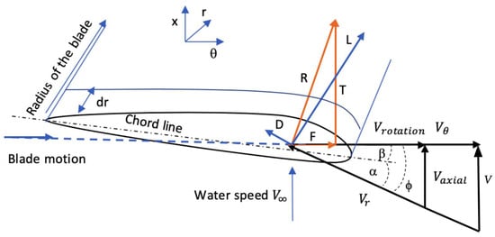
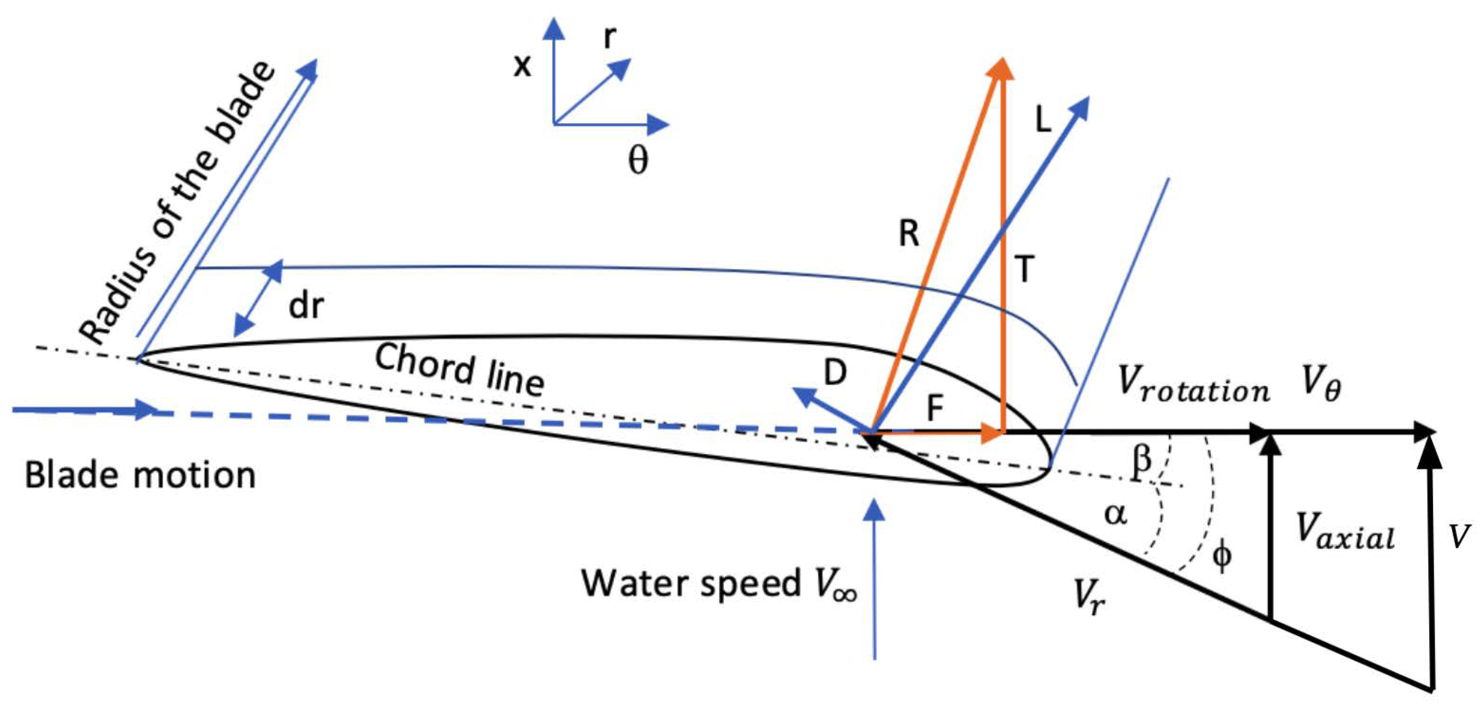
Blade Element Theory (BET) is a widely used approach to model the hydrodynamic forces acting on turbine blades by discretizing each blade into multiple elements along its span [39]. For each blade element, forces are calculated using the lift and drag characteristics of a two-dimensional airfoil profile. Figure 1 shows the flow velocity component and angles on the blade element.

Figure 1. Representation of velocity component and angles on the blade element [40].

In the rotor model the blade loading is first evaluated on each annular ring and then converted into a force per unit volume that can be added to the momentum equations of the CFD solver. Because the rotor has a finite number of blades, the ideal 2D loading must be reduced near the tip. This is done with Prandtl’s tip-loss factor $F_{\mathrm{tip}}$, which depends on the blade number n, the local radius r and the inflow angle $\varphi$:

$$F_{\mathrm{tip}}={\displaystyle \frac{2}{\pi }}arccos\left[exp\left(-{\displaystyle \frac{n(R-r)}{2rsin\varphi }}\right)\right],$$

where R is the rotor radius.

For a blade element of chord c, span $dr$, relative velocity $V_r$ and water density $\rho$, the sectional lift and drag are

$$\begin{array}{cc}\hfill L& ={\displaystyle \frac{1}{2}}\rho c{V}_r^2{C}_L{F}_{\mathrm{tip}},\hfill \end{array}$$

(14)

$$\begin{array}{cc}\hfill D& ={\displaystyle \frac{1}{2}}\rho c{V}_r^2{C}_D,\hfill \end{array}$$

(15)

with $C_L\left(\alpha \right)$ and $C_D\left(\alpha \right)$ taken from the airfoil polars and $\alpha$ the local angle of attack. The relative velocity is linked to the axial inflow and the blade rotation through

$$V_r=\sqrt{V_{\mathrm{axial}}^2+{\left(\omega r-V_{\theta }\right)}^2}$$

(16)

To make the forces act in the rotor directions, lift and drag are projected onto the axial (x) and azimuthal ($\theta$) axes.

$$\begin{array}{cc}\hfill f_x& =Lcos\varphi +Dsin\varphi ,\hfill \end{array}$$

(17)

$$\begin{array}{cc}\hfill f_{\theta }& =-Dcos\varphi +Lsin\varphi .\hfill \end{array}$$

(18)

Here $f_x$ produces thrust and $f_{\theta }$ produces torque. These are forces per unit blade span and must be distributed over the annular control volume occupied by the rotor in the mesh. For an annulus of circumference $2\pi r$ and numerical thickness e, the volume forces added to the momentum equations are

$$\begin{array}{cc}\hfill S_x& =-{\displaystyle \frac{n{f}_x}{2\pi re}},\hfill \end{array}$$

(19)

$$\begin{array}{cc}\hfill S_{\theta }& =-{\displaystyle \frac{n{f}_{\theta }}{2\pi re}},\hfill \end{array}$$

(20)

where n is the number of blades. The minus sign indicates that the fluid loses momentum while the rotor gains it.

These expressions are implemented in OpenFOAM (here through fvOptions). At every time step the local flow ($V_{\mathrm{axial}}$, $\omega$, and the induction factors supplied by the BET loop) is used to update $V_r$, then lift and drag from (14) and (15), then the projections (17) and (18), and finally the volume sources (19) and (20). In this way the turbine forcing remains consistent with the instantaneous CFD solution.

2.3. Numerical Implementation of Blade Element Theory in OpenFOAM

The implementation of Blade Element Theory (BET) within the OpenFOAM environment involves introducing momentum source terms into the fluid momentum equations, representing the forces exerted by the turbine blades on the flow. These source terms are distributed across the cells that compose the rotor disk region. OpenFOAM’s object-oriented C++ framework facilitates this by employing the basicSource abstract class, which serves as a template for various source term models. The BET implementation is encapsulated within the rotorDiskSource class, which contains the data and member functions necessary to calculate blade forces and corresponding momentum sources based on turbine parameters such as rotational speed, blade pitch, and geometry. The rotorDiskSource class is activated during simulation runtime when an appropriate entry is specified in the fvOptions dictionary, typically located in the case’s system directory.

Modifications to the rotorDiskSource Class

In order to enhance the accuracy and applicability of the BET model within the SedFoam solver, several critical modifications were implemented in the file of rotorDiskSourceTemplates.C, where the core source term calculations reside. These modifications address limitations in the original implementation as follows:

• Correction of Local Force Calculations:
  The original code incorrectly associated blade lift with axial forces and blade drag with tangential forces without considering the actual flow angle. This assumption is only valid when the flow angle is zero, which is generally not the case. The modification projects the lift and drag forces correctly onto the rotor axial and tangential directions using the local inflow angle, thereby ensuring accurate force vector decomposition [41].
• Generalized Blade Tip Loss Correction: Prandtl’s tip loss factor was implemented more comprehensively to better account for three-dimensional aerodynamic effects and vortex-shedding phenomena near blade tips. This correction improves the fidelity of the load distribution along the blade span and mitigates overprediction of blade forces near the tips [41].

Collectively, these enhancements significantly improve the predictive capability of the BET model within OpenFOAM, yielding more accurate wake dynamics and sediment transport predictions downstream of tidal turbines.

2.4. First-Order Wave Theory (FOWT)

The solution for the shallow water approximation gives us the horizontal and vertical velocity equations [42]. The velocity components u and v of the wave motion are given by

$$u={\displaystyle \frac{A\omega }{kH}}cos(kx-\omega t)$$

(21)

$$v={\displaystyle \frac{A\omega }{H}}ysin(kx-\omega t)$$

(22)

where the vertical coordinate y varies from the bottom at $y=0$ to the free surface at $y=H$, i.e.,

$$0\le y\le H.$$

The wave-induced pressure perturbation $p_w$ (relative to hydrostatic) follows from the free-surface elevation ${\displaystyle \eta (x,t)=Acos(kx-\omega t)}$, namely:

$$p_w=\rho gAcos(kx-\omega t)=\rho g\eta$$

(23)

Here, A is the wave amplitude, $\omega$, the angular frequency, k, the wavenumber, H, the total water depth, x, the horizontal coordinate, y, the vertical coordinate (measured upward from the bottom), t, time, $\rho$, fluid density, and g, gravitational acceleration.

In incompressible flow the full Navier–Stokes momentum equation is equal to

$$\rho \left({\partial }_t\mathit{u}+\mathit{u}·\nabla \mathit{u}\right)=-\nabla p+\mu {\nabla }^2\mathit{u}+\rho \mathit{g},$$

(24)

where $\mathit{u}=(u,v)$, p is the total pressure, and $\mu$ the dynamic viscosity. We decompose the pressure in hydrostatic one, wave pressure and non-hydrostatic pressure as:

$$p=p_{\mathrm{hydrostatic}}+p_w+p^{\prime }.$$

Thus, the wave-induced pressure enters the momentum balance as a source term, or equivalently as a body force ${\displaystyle {\mathit{F}}_{\mathrm{wave}}=-\nabla p_w}$

$${\mathit{F}}_{\mathrm{wave}}=-\nabla p_w=-\rho gA\left[\begin{array}{c}-ksin(kx-\omega t)\\ 0\end{array}\right]$$

(25)

The momentum equation is at the end as (26) with a body wave force imposed throughout the domain.

$$\rho \left({\partial }_t\mathit{u}+\mathit{u}·\nabla \mathit{u}\right)=-\nabla p^{\prime }+\mu {\nabla }^2\mathit{u}+{\mathit{F}}_{\mathrm{wave}},$$

(26)

In the shallow-water limit ($H/\lambda \ll 1$), the pressure field remains essentially hydrostatic, and vertical accelerations are vanishingly small (since v is small). For this reason these motions are often called “hydrostatic waves”. In practice, a pressure sensor installed on the seabed will directly record these wave-driven pressure variations [42].

3. Model Validation

3.1. Validation of Numerical Implementation of BET

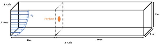
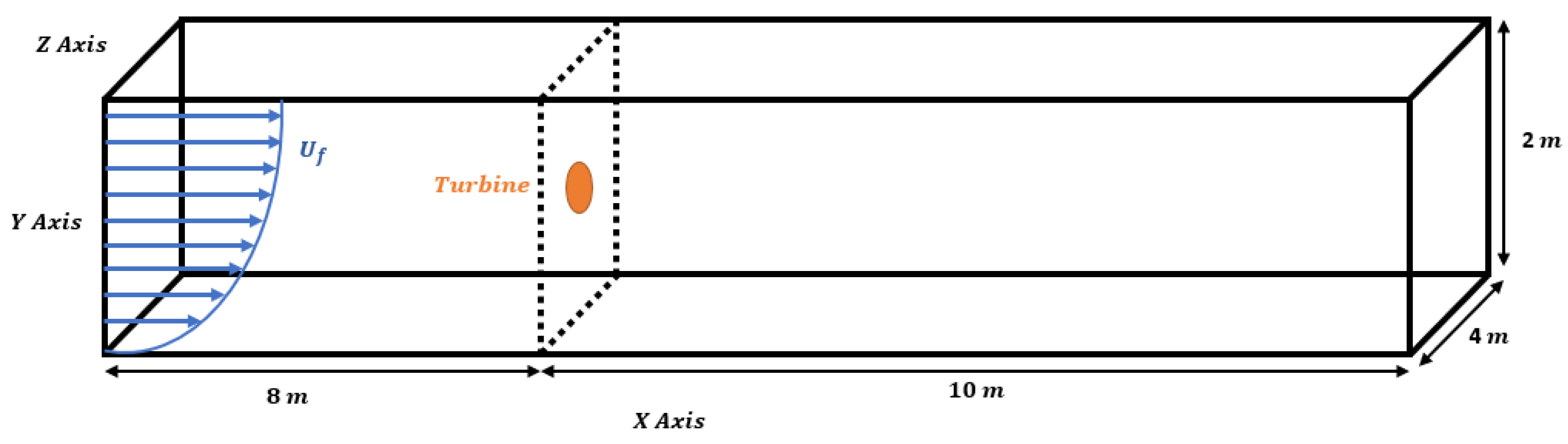
In this section, the Blade Element Theory (BET) actuator-disk model implemented in OpenFOAM is validated against the experimental measurements of Mycek et al. [22]. The experiments were performed in the IFREMER water-tunnel facility, which is 18 m long, 4 m wide, and 2 m deep. The tested turbine had a rotor diameter d of 0.7 m and a hub diameter of 0.092 m. The rotor blades were based on the NACA 63418 airfoil profile and operated under a uniform inflow with a free-stream velocity of $U_{\infty }=0.8\mathrm{m}/\mathrm{s}$ and turbulence intensity $\mathrm{TI}=3\%$. The operating point corresponded to a tip-speed ratio of $\mathrm{TSR}=3.67$ and a Reynolds number of $\mathrm{Re}=2.8\times {10}^5$, with a blade pitch angle of $0^{\circ }$ and counterclockwise rotation.

The numerical domain was built to match the dimensions of the experimental tunnel ($18\mathrm{m}\times 4\mathrm{m}\times 2\mathrm{m}$) using the blockMeshDict utility in OpenFOAM, as illustrated in Figure 2. The rotor-swept area, represented here as an actuator disk, was generated using Gmsh [43]. The mesh was then locally refined in the vicinity of the rotor using snappyHexMeshDict to better resolve the wake development and improve the accuracy of the predicted flow features.

Figure 2. Computational domain and turbine setup replicating the Mycek et al. [22] configuration.

To apply the turbine forcing terms, the rotor disk cells were selected using the topoSetDict utility, which then enabled source terms to be applied via the fvOptions dictionary during simulation.

Boundary Conditions for BET Case Only

Boundary conditions were carefully applied to represent physical scenarios realistically:

• Bottom boundary: No-slip condition, replicating the realistic frictional interaction with the seabed.
• Top boundary: Slip condition, reflecting the free-surface approximation for air–water interfaces.
• Lateral boundaries (front and back): Symmetry planes to reduce computational load without sacrificing accuracy, and also to act like a slip condition.
• Inlet boundary: Specified velocity inlet condition with current velocities.

  $${\displaystyle \frac{u^f}{u_{\ast }}}={\displaystyle \frac{1}{\kappa }}ln\left({\displaystyle \frac{z+z_0}{z_0}}\right)$$

  (27)

  where $u_{\ast }$ is the bed friction velocity equal to $u_{\ast }=0.038$ m/s for $U_{ref}=0.77$ m/s and $z_{ref}=0.2$ m, $\kappa$ is the von Kármán constant equal to 0.41. While in the case of sedFoam solver the $z_0$ is taken as $2.5\times d_s$. Where $d_s$ represents the sediment diameter.
• Outlet boundary: For pressure uniform Dirichlet condition was imposed. p was fixed to zero at the outlet boundary. For all other quantities the zero-gradient condition was applied.

At the top boundary, we applied a slip condition because the present configuration does not resolve a deforming free surface (rigid-lid approximation). The wave effect was introduced through prescribed inlet kinematics and an oscillatory pressure-gradient/body-force term. Therefore, imposing a shear-free condition at the top avoids generating an artificial boundary layer at the upper boundary and keeps the focus on near-bed dynamics, which control sediment motion and scour.

To accurately capture the near-wake structure, two distinct modeling approaches were compared: a ’No Hub’ case and a ’With Hub’ case. In the ’With Hub’ configuration, the hub is represented as a physical cylindrical boundary. The no-slip boundary condition was imposed on its surface by using $snappyHexMesh$. This allows the model to resolve the physical blockage and the resulting pressure-driven deficit at the center of the wake. In contrast, the BET source terms are applied only to the cells within the surrounding annular region swept by the blades.

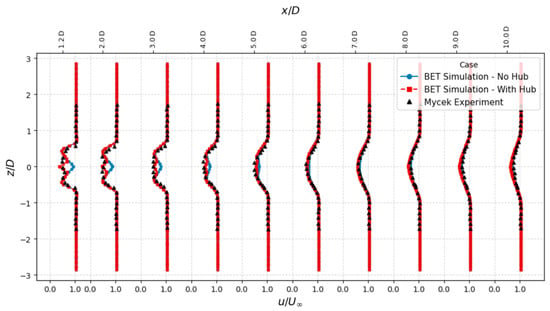
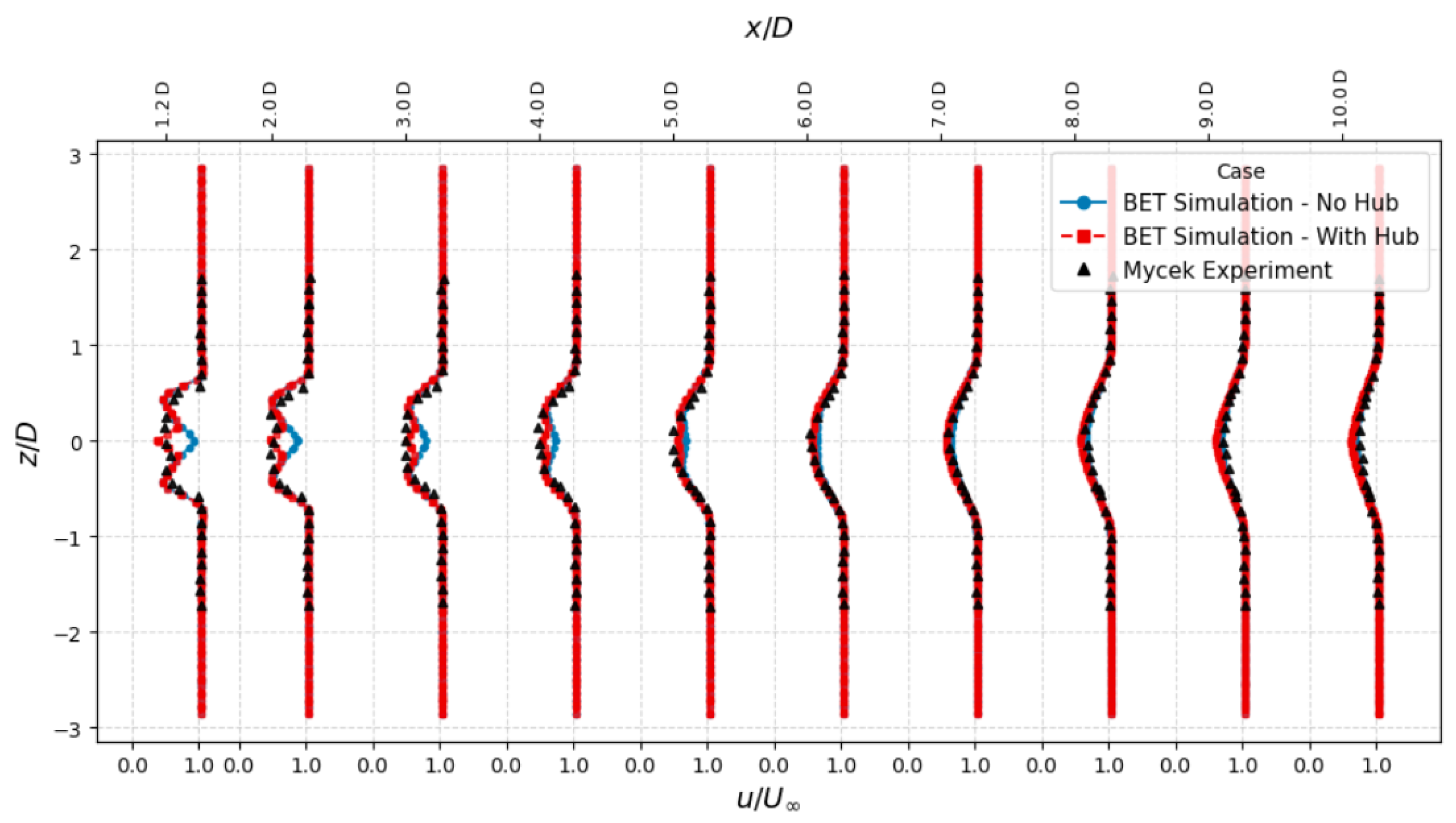
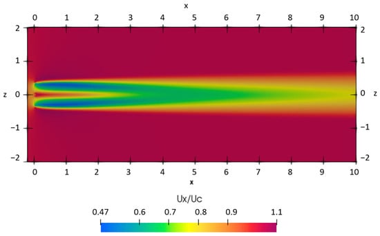
After running the simpleFoam solver to compute the wake field. We got the results as shown in Figure 3. We can see that the result in the case of the hub, considering it as a solid (no-slip condition), gives a good result and overlaps with the experimental results of [22].

Figure 3. Comparison between experimental and numerical axial direction wake-flow velocity along the width (z-axis) of the tank. The experimental case conducted by [22] is used with 0.8 stream velocity and 3% turbulence intensity.

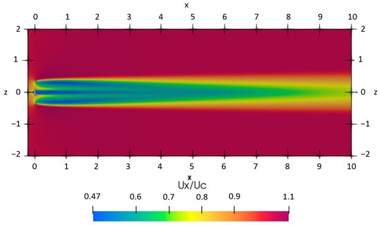
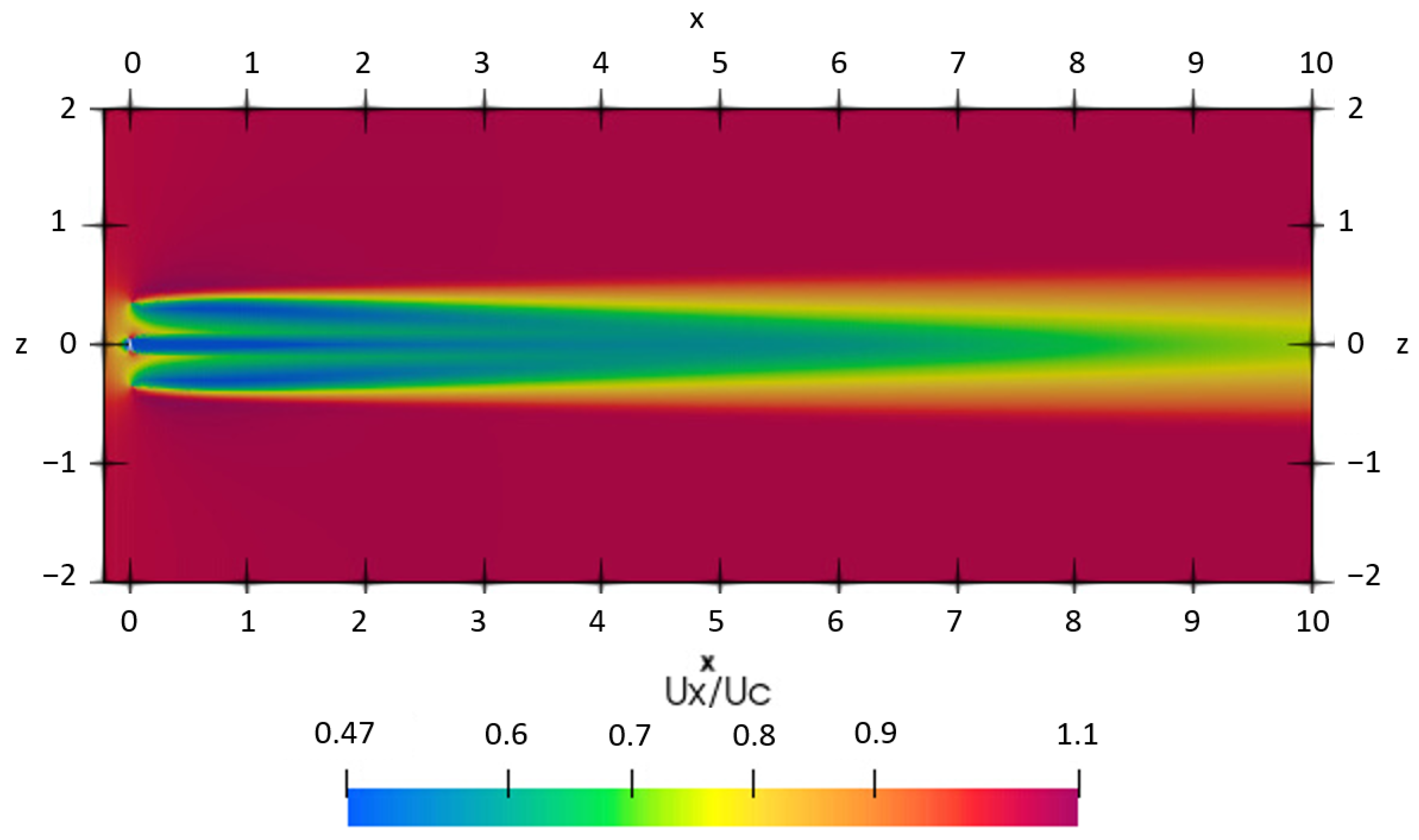
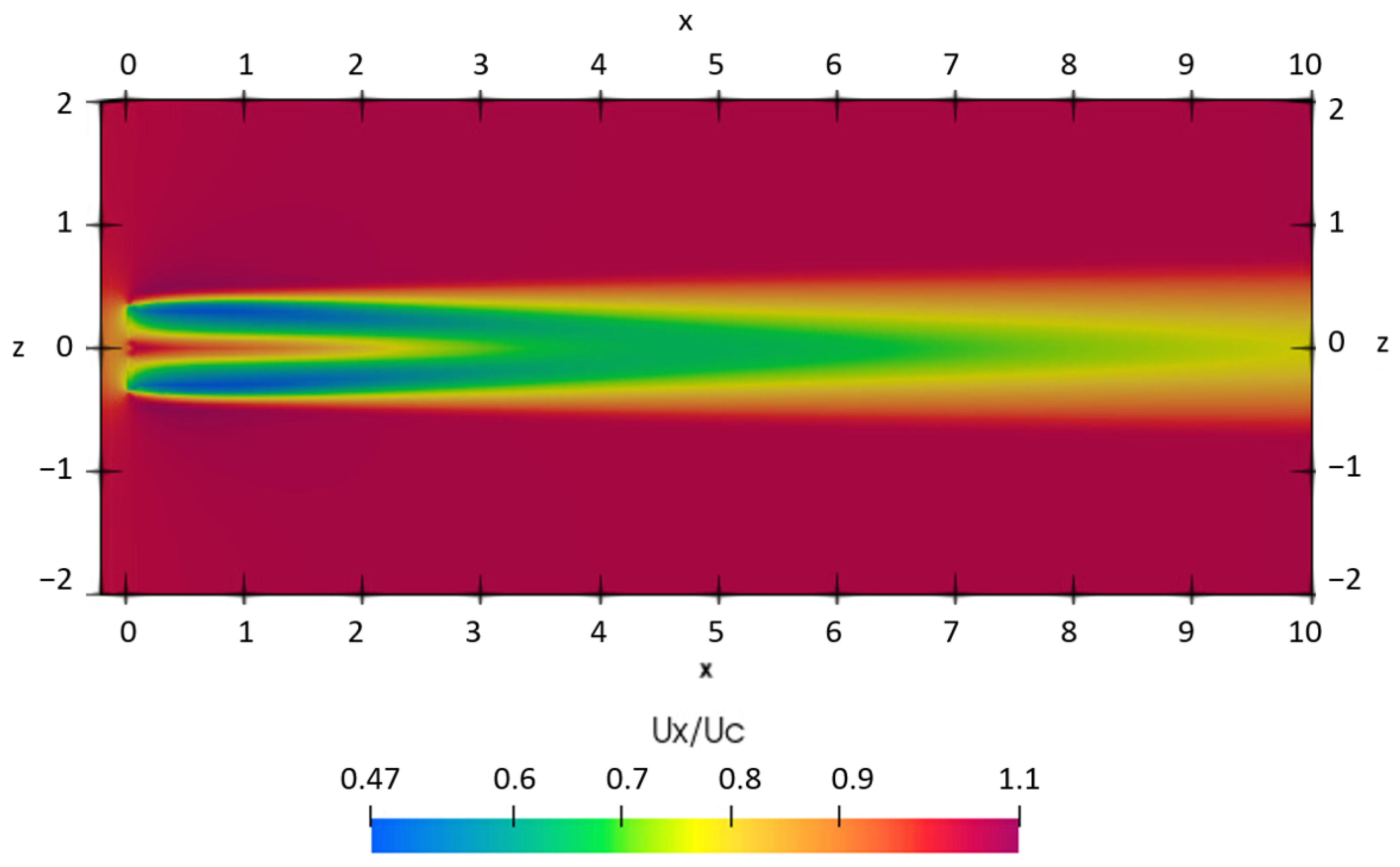
Figure 4 and Figure 5 show maps of the normalized axial velocity $U_x/U_c$ in a plane through the rotor hub height. Two thin low-speed filaments leave the rotor near the tip region and roll into the main wake. These correspond to the strong shear layers produced by the blades (tip vorticity), which gradually merge downstream. In the case of the hub (Figure 4), the near-wake deficit is deeper right behind the rotor and remains coherent for a longer distance. The 0.7–0.8 $U_c$ band extends farther downstream before the wake begins to recover, which is consistent with the extra blockage introduced by the hub and the stronger shear near the mid-plane.

Figure 4. Normalized axial velocity field $U_x/U_c$ in the x–z plane including hub.

Figure 5. Normalized axial velocity field $U_x/U_c$ in the x–z plane without hub.

In the case of no hub (Figure 5), the wake is smoother and recovers slightly faster. The same 0.7–0.8 $U_c$ band contracts earlier, and the deficit is less pronounced near the centerline. In other words, the flow has an easier path through the rotor center when no solid hub is present, so mixing with the outer flow starts sooner.

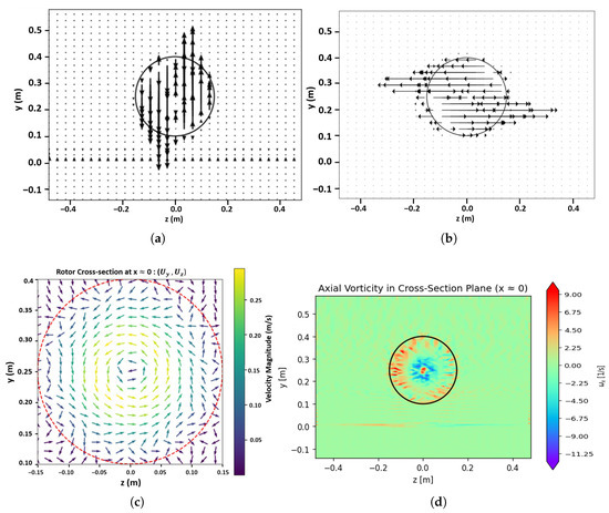
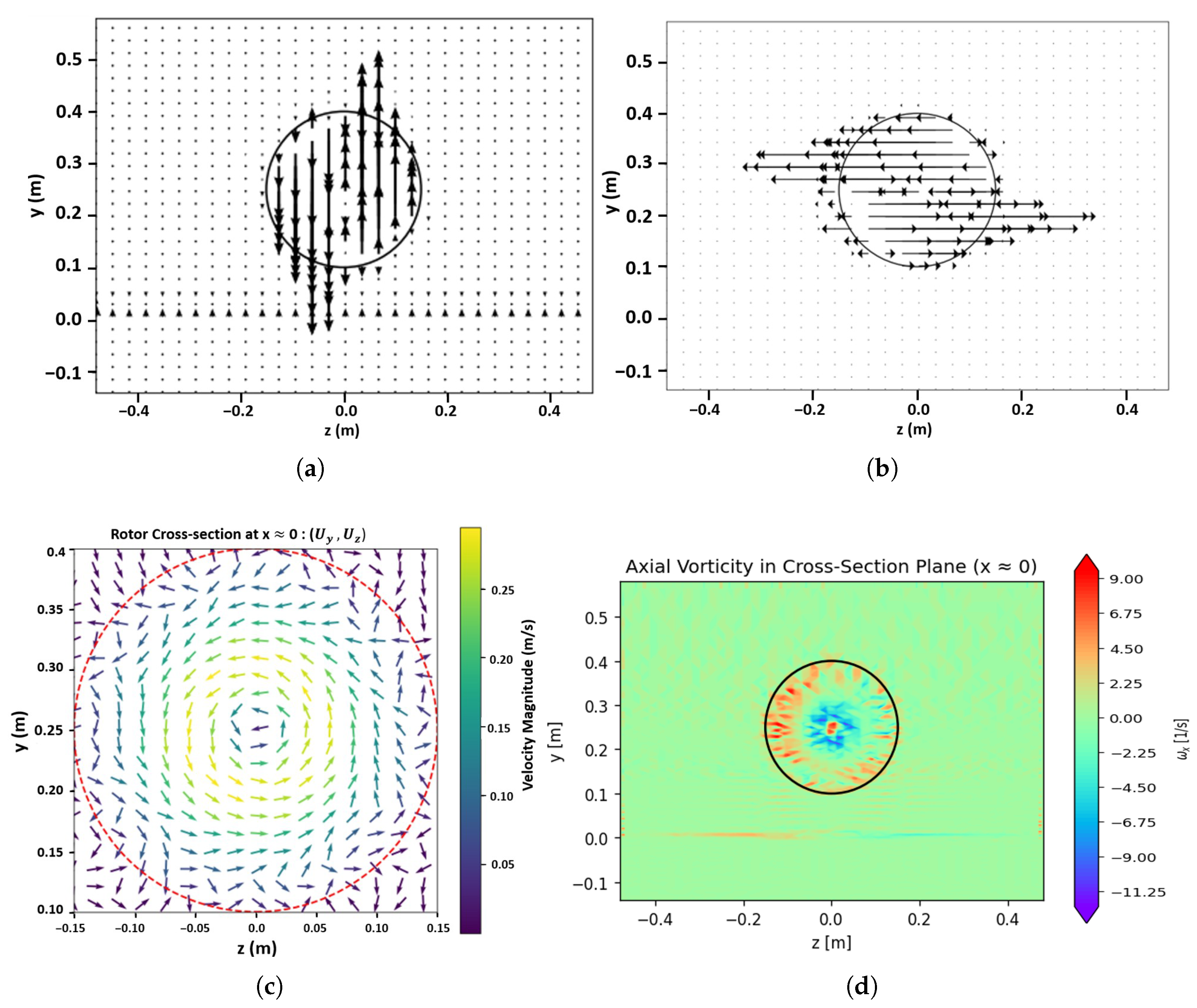
Figure 6 shows the swirl of the rotating rotor in a counterclockwise direction. Figure 6a shows the vector of the vertical component of the velocity. We can see that the velocity vectors are distributed across the rotor in a way that causes the rotor to rotate in a counterclockwise direction. Similarly, Figure 6b shows the vector of the spanwise component of the velocity. The vector weakens near the tip and hub, which is consistent with the tip loss. Lastly, Figure 6c shows the combined effect of the vertical and spanwise components of the velocity. Figure 6d shows the axial vorticity, computed as ${\omega }_x=\partial U_z/\partial y-\partial U_y/\partial z$ and plotted in the y–z cross-section where as the circle marks the rotor circumference. ${\omega }_x$ measures local swirl about the streamwise (x) axis. We can see in this figure that the vorticity is higher at the edge of the blades and outside of the domain of the rotor the vorticity tends towards zero. All those figures show that the velocity vector accurately represents the rotation and hence validates the BET model implementation.

Figure 6. Cross-section through the rotor disk ($x\approx 0$). The circle marks the rotor circumference. Panels: (a) vertical velocity $U_y$; (b) spanwise velocity $U_z$; (c) combined vector field $(U_y,U_z)$ in the y–z plane; (d) axial vorticity in (y-z) plane.

3.2. Validation of Numerical Implementation of FOWT

In order to accommodate the wave effect in the model, the velocity of the marine current at the inlet was added to the velocity components of u (Equation (21)) and v (Equation (22)) from the wave motion equations. Furthermore, the wave-induced pressure force (Equation (25)) was added into the momentum equation by using fvOption in OpenFoam. The parameters that were used in the simulation are mentioned in Table 1.

Table 1. Wave parameters used in the simulations (from fvOptions) and derived quantities.

Quantity	Symbol	Value	Unit
Amplitude	A	0.03	m
Wavenumber	k	2.837	m−1
Angular frequency	$\omega$	6.283	s−1
Gravity	g	9.81	m s−2
Fluid density	$\rho$	1000	kg m−3
Wavelength ($\lambda =2\pi /k$)	$\lambda$	2.21	m
Period ($T=2\pi /\omega$)	T	1.00	s
Frequency ($f=\omega /2\pi$)	f	1.00	Hz
Phase speed ($c=\omega /k=\lambda /T$)	c	2.21	m s−1

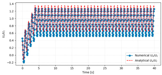
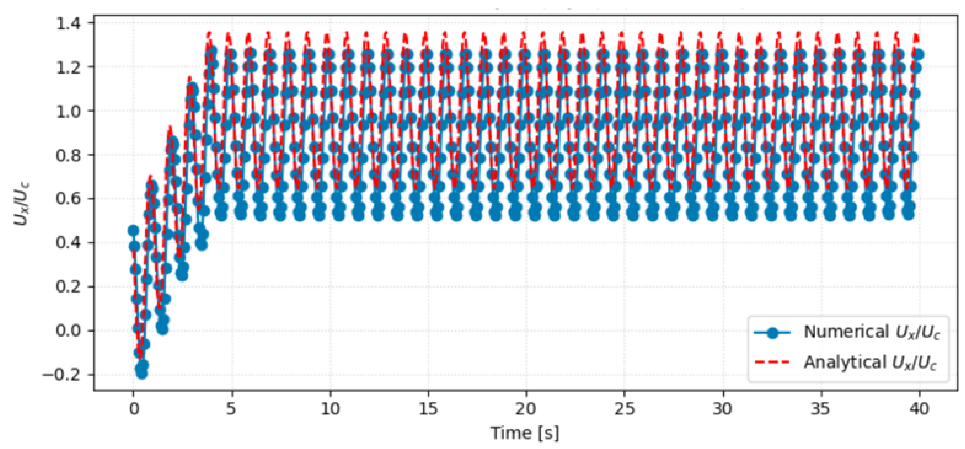
After running the simulation, we got the result as shown in Figure 7. From the figure we can see that the numerical and analytical results are very close to each other and satisfy our model accuracy. The little change is due to the fact that in the analytical solution, the viscous effect is not considered, while in the case of the numerical results, the viscous effect is considered.

Figure 7. Comparison of wave–current-induced hydrodynamics cross-sectional average flow velocity in x direction near the inlet.

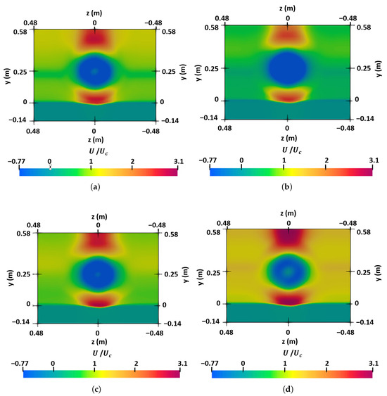
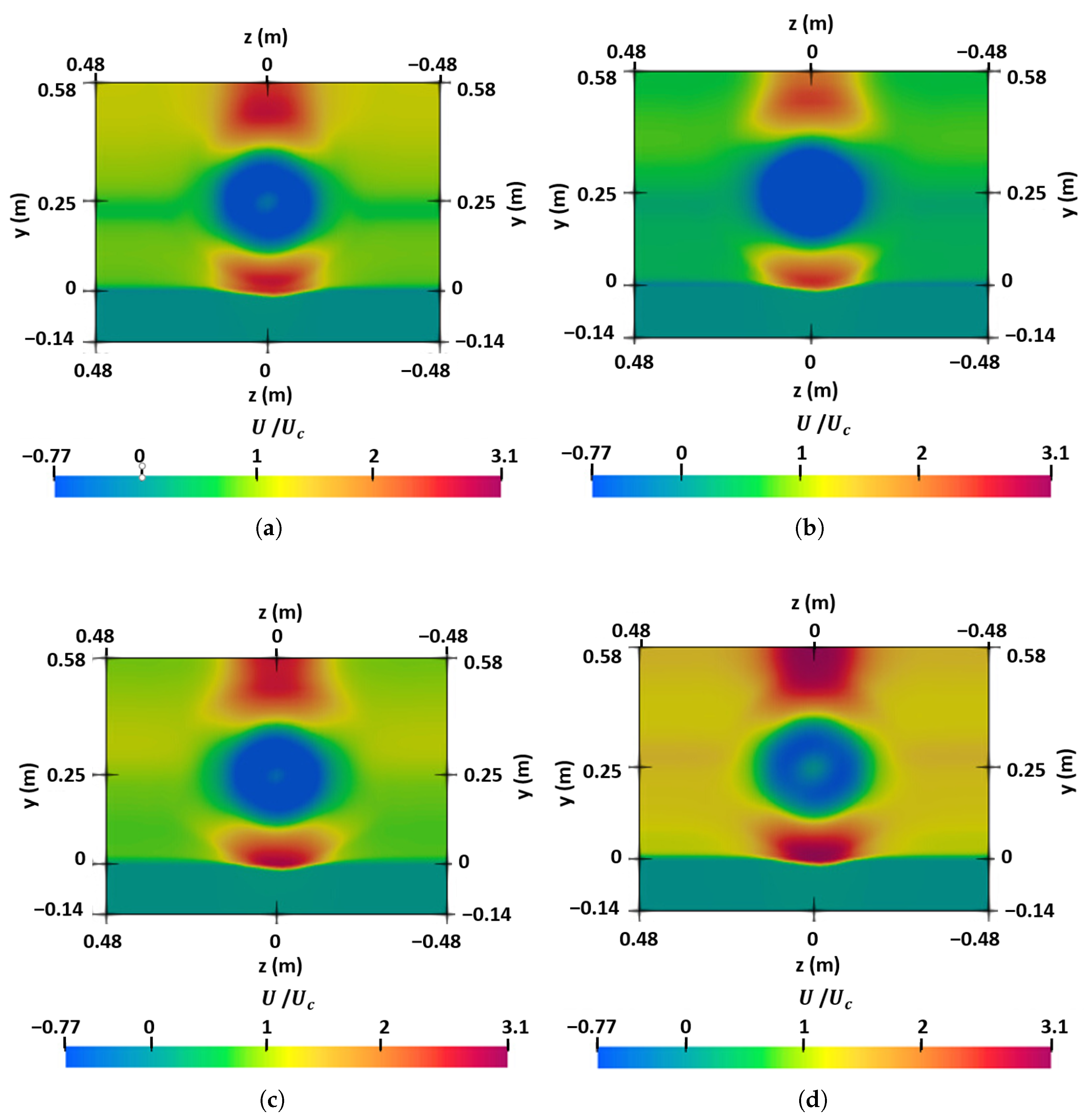
For further validation of wave forcing, the cross-sectional field of normalized axial velocity $U_x/U_c$ at four instants over roughly one wave cycle ($t=9.25,9.50,9.75,10.00$ s) is captured as shown in Figure 8. The color scale is fixed across frames. The blue color indicates the velocity deficit. We observe a periodic acceleration and deceleration (red/green lobes grow and decay) in step with the wave phase, while the wake retains its shape. This sinusoidal amplification and reversal from one frame to the next is exactly what first-order wave theory predicts for the horizontal velocity perturbation, confirming that the implemented wave body-force term imposes the correct phase and magnitude of the wave-induced motion.

Figure 8. Temporal evolution of normalized axial velocity $U_x/U_c$ in the y–z plane over one wave phase (same color scale in all frames): (a) $t=9.25\mathrm{s}$; (b) $t=9.5\mathrm{s}$; (c) $t=9.75\mathrm{s}$; (d) $t=10\mathrm{s}$.

The wave body-force formulation used in this study is applied uniformly across the computational domain as a simplified approach for modeling the effects of wave-induced forces on sediment transport and seabed evolution. This formulation is based on the assumption that the wave-induced motion can be adequately represented by a sinusoidal velocity perturbation (first-order wave theory) that applies uniformly across the depth of the domain. The choice of this approach is made to reduce computational complexity, as resolving the free surface and capturing detailed wave propagation effects would require a more computationally intensive two-phase flow model. The absence of a resolved free surface is offset by the use of an effective wave body force that captures the essential characteristics of wave-induced motion, including the phase and magnitude of velocity perturbations, which are sufficient for the current study’s objectives.

4. Implementation of Both BET and FOWT in SedFoam Solver

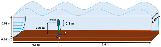
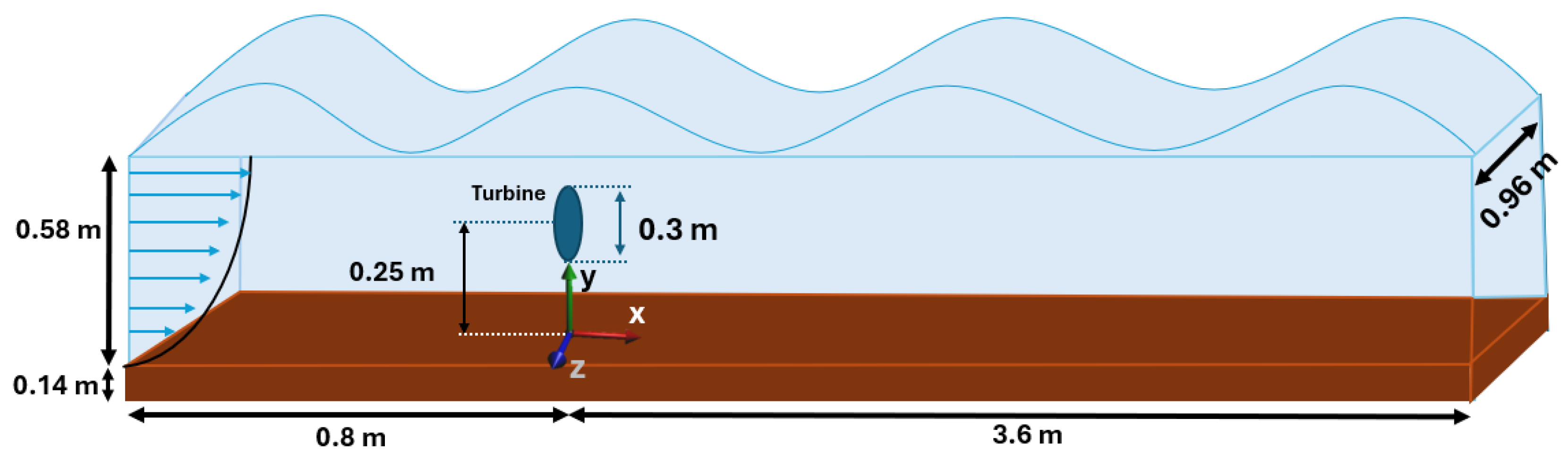
After verifying Blade Element Theory (BET) and First-Order Wave Theory (FOWT) independently, both source terms were combined in SedFoam-2.0 to study their coupled effect on sediment transport and scour. Figure 9 shows the full computational setup.

Figure 9. Computational domain for combined BET + FOWT simulations. The total length is 4.4 m, the mobile sediment layer is 0.14 m thick, and the overlying water column is 0.58 m deep. The turbine rotor (diam. 0.30 m) is centered at $x=0.8$ m and hub height $y=0.25$ m. Coordinate axes: x downstream, y vertical from the bed, z lateral.

• Domain and mesh setup:
  • A rectangular block of dimensions $4.4\times 0.62\times 0.96$ m was created via blockMeshDict.
  • The lower 0.14 m contains mobile sediment (61% volume fraction at the bottom), above which lies 0.58 m of clear water.
  • The turbine geometry (STL) was snapped into the mesh at $x=0.8$ m using snappyHexMeshDict, and rotor cells were marked with topoSetDict.
• Volumetric source terms (in fvOptions):
  • BET source: axial and tangential forces distributed over “rotorCells” (Section 2.2).
  • FOWT source: wave body force

    $${\mathit{F}}_{\mathrm{wave}}(x,t)=-\nabla p^{\prime }=-\rho gA\left(-ksin(kx-\omega t),0,0\right)$$

    applied to all cells.
• Boundary and initial conditions:
  • Inlet ($x=0$): uniform current $U_{\infty }$ plus wave kinematics

    $$u=U_{\infty }+{\displaystyle \frac{A\omega }{kH}}cos(kx-\omega t),v={\displaystyle \frac{A\omega }{H}}ysin(kx-\omega t).$$
  • Outlet ($x=4.4$ m): Dirichlet pressure $p=0$; zero-gradient for other variables.
  • Bottom ($y=0$): no-slip for the fluid; granular stress models for the sediment.
  • Free surface ($y=0.58$ m): slip condition.
  • Lateral (z-faces): symmetry planes.
• Solver settings:
  • sedFoam_rbgh run unsteadily with the Euler time scheme.
  • The time step $\Delta t={10}^{-4}$ s was selected to ensure numerical stability and accurate resolution of the transient flow. Based on the maximum flow velocity (0.5 m/s) and the smallest grid spacing near the bed and rotor ($\Delta x=1\times {10}^{-4}$ m); this choice maintains the Courant number well below unity throughout the domain.
• Model parameters used in this study:
  • Rheology and dense-suspension constants (sand):

    $$\begin{array}{cccccc}\hfill {\varphi }_{max}& =0.625,\hfill & \hfill {\mu }_s& =0.63,\hfill & \hfill {\mu }_2& =1.13,\hfill \\ \hfill I_0& =0.60,\hfill & \hfill B_{\varphi }& =0.66,\hfill & \hfill n& =2.50,\hfill \\ \hfill \mathrm{Dsmall}& ={10}^{-4},\hfill & \hfill \mathrm{relaxPa}& =5\times {10}^{-5}.\hfill \end{array}$$
  • Code switches:

    $$\begin{array}{cc}\mathtt{granularRheology}\hfill & \mathtt{on}\hfill \\ \mathtt{granularDilatancy}\hfill & \mathtt{off}\hfill \\ \mathtt{granularCohesion}\hfill & \mathtt{off}\hfill \\ \mathtt{FrictionModel}\hfill & \mu \left(I\right)\hfill \\ \mathtt{PPressureModel}\hfill & \mu \left(I\right)\hfill \\ \mathtt{FluidViscosityModel}\hfill & \mathtt{BoyerEtAl}\hfill \end{array}$$
  • These settings activate the Boyer–Guazzelli–Pouliquen viscous-number law for dense suspensions while using the $\mu \left(I\right)$ frictional rheology for the granular phase.
• Coupling strategy.
  • At each time step, solve the two-phase flow with BET forcing, update ${\mathit{F}}_{\mathrm{wave}}$ from the analytical pressure $p_w$ (Equation (23)), then iterate the PIMPLE loop.
  • The coupled field captures turbine wakes and oscillatory wave forcing that drive sediment transport and scour.
• Tip-speed ratio (TSR):
  • Three operating points: TSR $=3.6$, 5, and 9.
• Numerical schemes:
  • First-order: Euler (time).
  • Second-order: Gauss linear (gradients), linear (interpolation), Gauss linear corrected (laplacians).
  • Bounded/limiters: limitedLinear01 (divergence), cellLimited Gauss linear 1 (gradients of k, $\epsilon$, $\omega$).

With this setup, SedFoam captures both the steady turbine-induced turbulence and the oscillatory forcing from surface waves, allowing for detailed prediction of scouring patterns under combined wave–current conditions.

5. Results and Discussion

The simulation results explicitly highlight significant variations in sediment dynamics due to the presence of wave forces, offering profound insights into sediment transport behaviors under different hydrodynamic conditions.

5.1. Normalized Axial Velocity Field

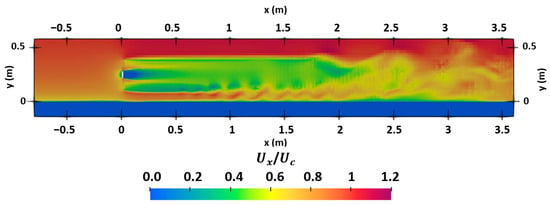
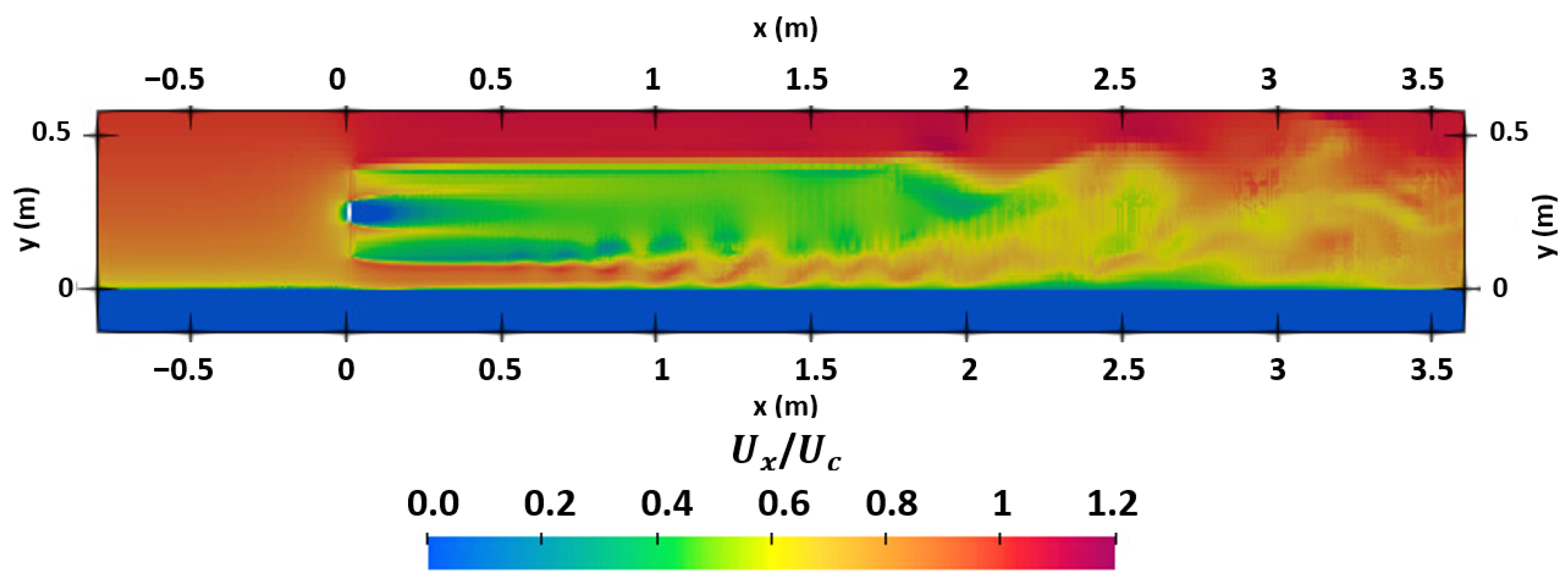
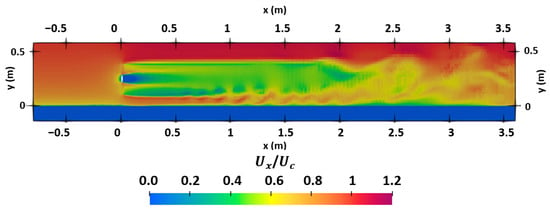
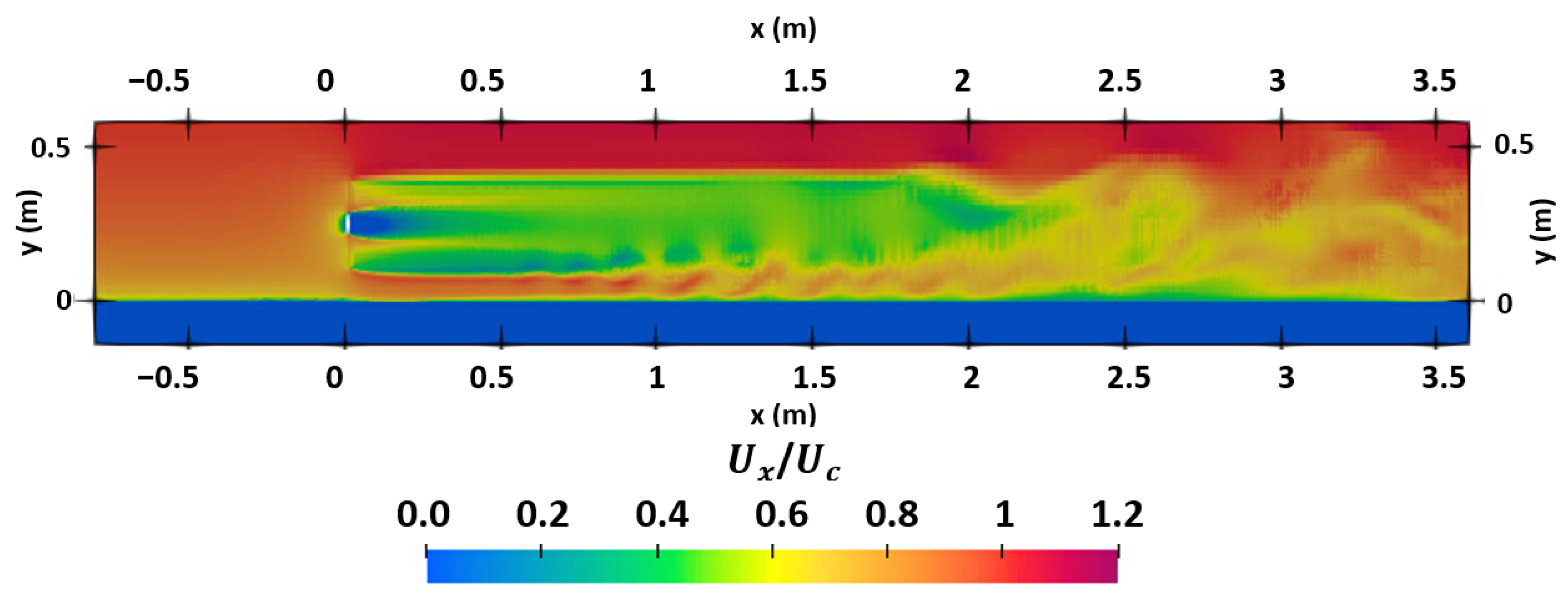
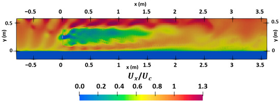
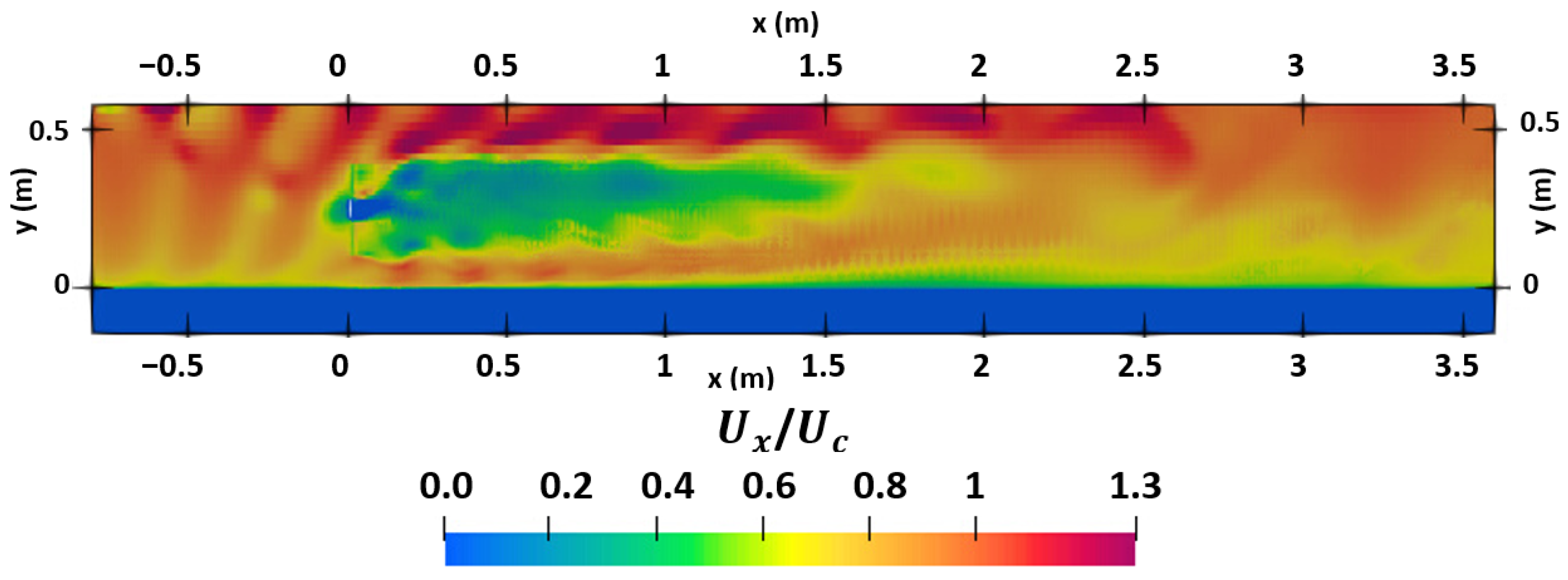
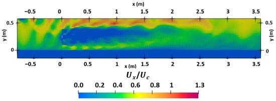
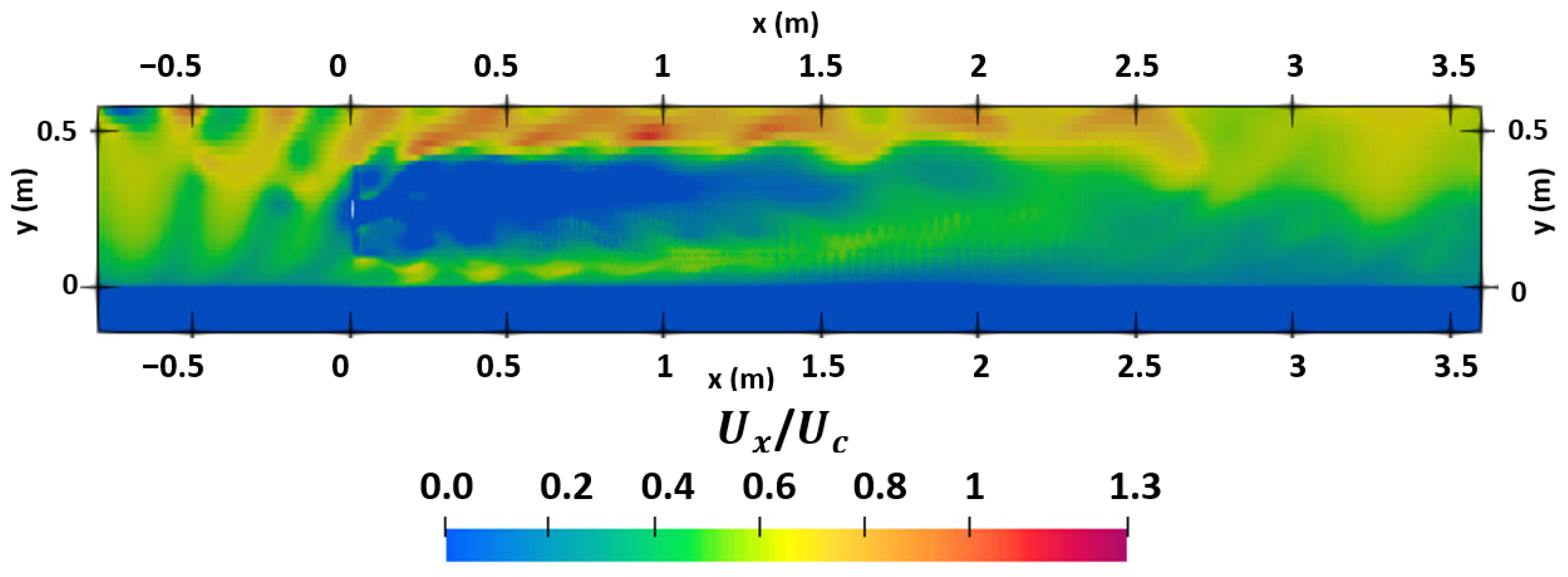
Figure 10 and Figure 11 show the normalized axial velocity field $U_x/U_c$ in the x–y plane for the marine current–only case at $t=19.25$ s and $t=19.5$ s, respectively. Figure 12 and Figure 13 present the corresponding fields for the marine current + wave case at $t=19.25$ s (zero crossing) and $t=19.5$ s (wave trough), respectively. The rotor is located at $x\approx 0$, $y\approx 0.25$ m, and the dark-blue strip along the bottom represents the mobile sediment layer. In the current-only case (Figure 10 and Figure 11), a classic BET wake is observed, with a pronounced near-wake velocity deficit (green/blue) bounded by relatively smooth shear layers that recover gradually downstream; higher-velocity flow is mainly confined to the upper water column, while low speeds persist near the bed. When waves are included (Figure 12 and Figure 13), the upper water column accelerates and the shear layers become thicker and more undulatory, indicating enhanced mixing. The wake spreads laterally and recovers faster, while the near-bed low-speed band remains constrained by bottom friction.

Figure 10. Normalized axial velocity field $U_x/U_c$ in the x–y plane for marine current only case at $t=19.25$ s. (for TSR = 3.6).

Figure 11. Normalized axial velocity field $U_x/U_c$ in the x–y plane for marine current only case at $t=19.5$ s. (for TSR = 3.6).

Figure 12. Normalized axial velocity field $U_x/U_c$ in the x–y plane for marine current + wave case at $t=19.25$ s corresponds to the zero crossing. (for TSR = 3.6).

Figure 13. Normalized axial velocity field $U_x/U_c$ in the x–y plane for marine current + wave case at $t=19.5$ s corresponds to the wave trough. (for TSR = 3.6).

5.2. Wake Comparison

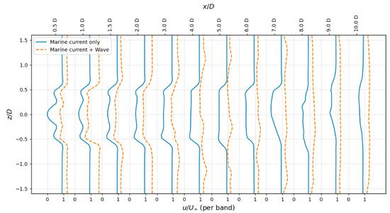
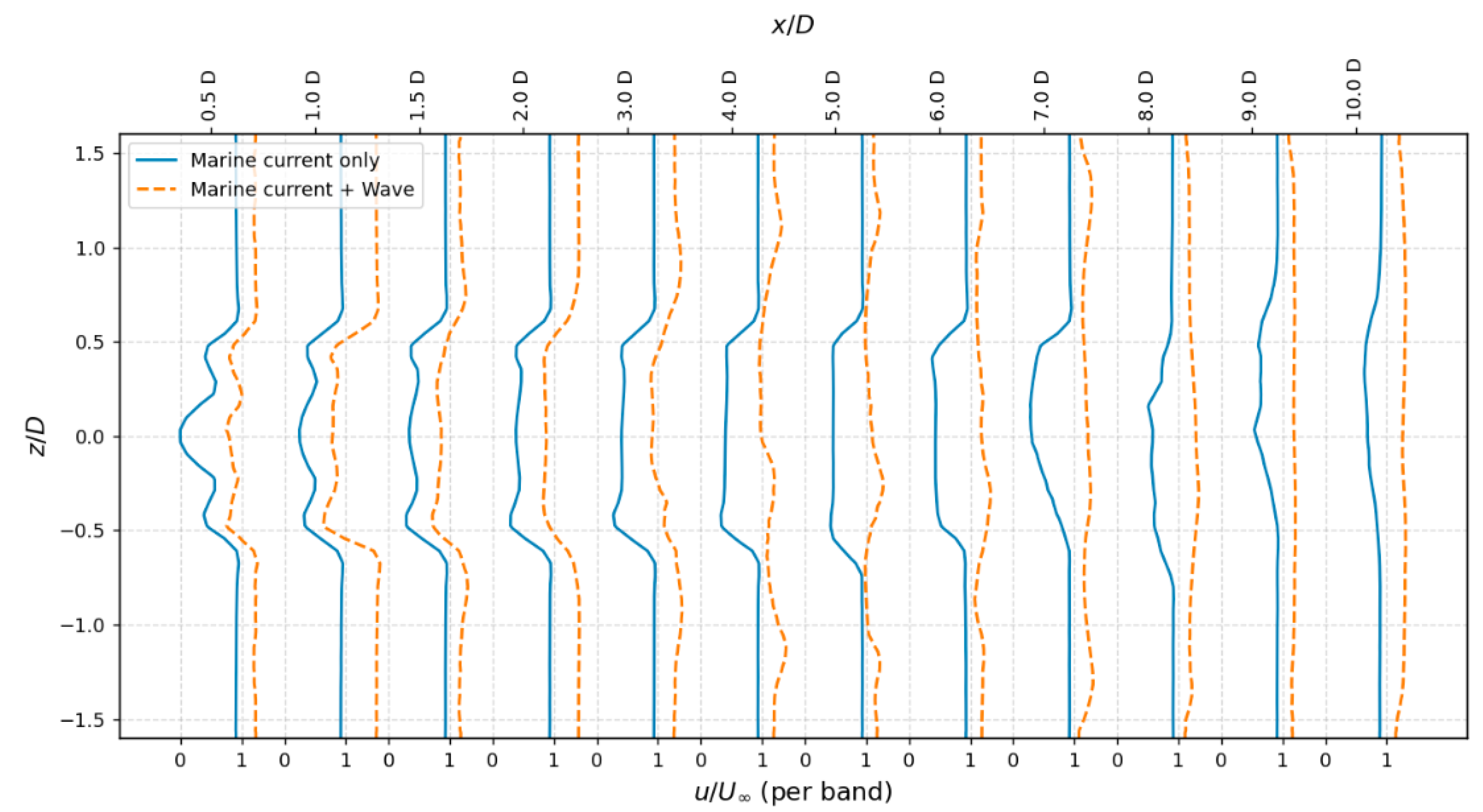
Figure 14 compares hub-height lateral profiles of the normalized axial velocity, $u/U_{\infty }$, at different locations of $x/D=0.5$–10 for the marine current case (solid blue) and the marine current-wave case (dashed orange). Each vertical “band” shows $u/U_{\infty }$ for a given $x/D$; the corresponding streamwise locations are indicated on the top axis. The profile at $x/D$ = 0.5 exhibits a local minimum near the centreline ($z/D=0$), reflecting the imprint of the hub. Later at the downstream the velocity is not zero because at these sections the flow has already begun to re-accelerate. In the near wake ($x/D\lesssim 2$) the wave–current case shows a slightly deeper and more confined deficit than the current-only case, consistent with the instantaneous acceleration imposed by the oscillatory wave forcing at the rotor. Farther downstream ($x/D\gtrsim 4$) the wave–current profiles lie systematically closer to unity across the span, indicating faster wake recovery. This behaviour is consistent with wave-induced mixing, which redistribute momentum into the wake and accelerate the decay of the velocity deficit. The progressive smoothing of the profile shapes with distance confirms that the combined wave–current forcing modifies both wake intensity and recovery rate, underscoring the importance of including waves in wake predictions.

Figure 14. Lateral wake profiles $u/U_{\infty }$ at $x/D=0.5$–10 for the Marine current only case (solid blue) and the Marine current + Wave case (dashed orange) at $t=20\mathrm{s}$ (for TSR = 3.6).

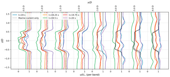
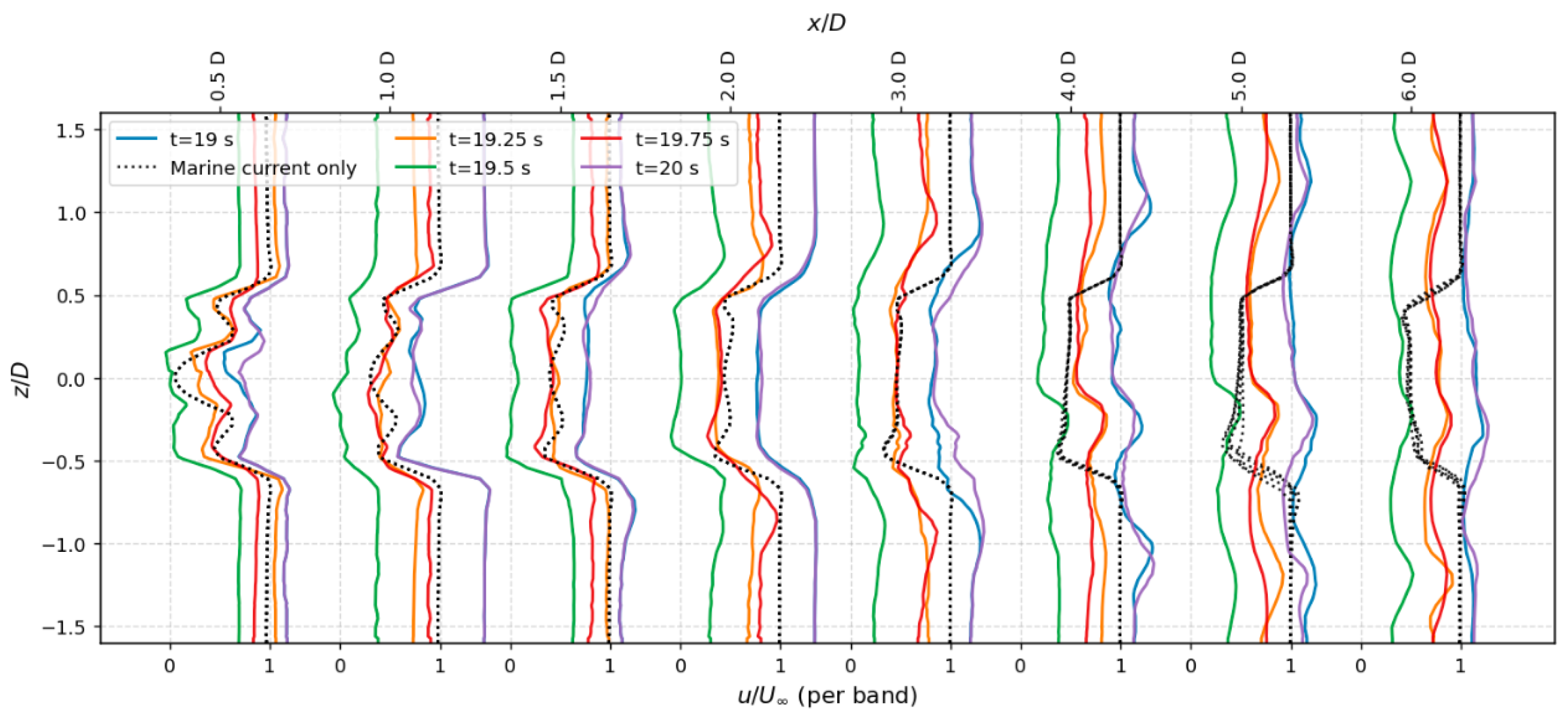
Figure 15 demonstrates that the instantaneous wake of the rotor is not stationary under wave–current forcing, but oscillates with the wave phase. The dotted black line represents the current only case. Within the first two diameters downstream, the lateral profiles swing between deeper and shallower deficits as the phase progresses from crest to trough, which alters the wake deficit. These differences decay rapidly with distance, and beyond about $4D$ the curves are nearly indistinguishable, showing that the effect of the phase quickly vanishes in the downstream of the turbine.

Figure 15. Wake profiles at five wave phases for TSR = 3.60, shown at $x/D=\{0.5,1.0,1.5,$$2.0,3.0,4.0,5.0,6.0\}$. Dotted black line represents a marine current only case.

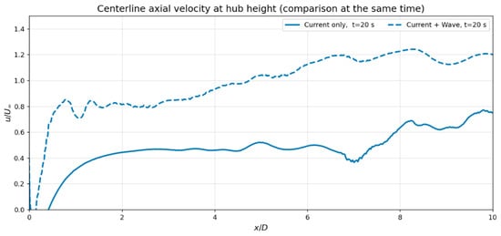
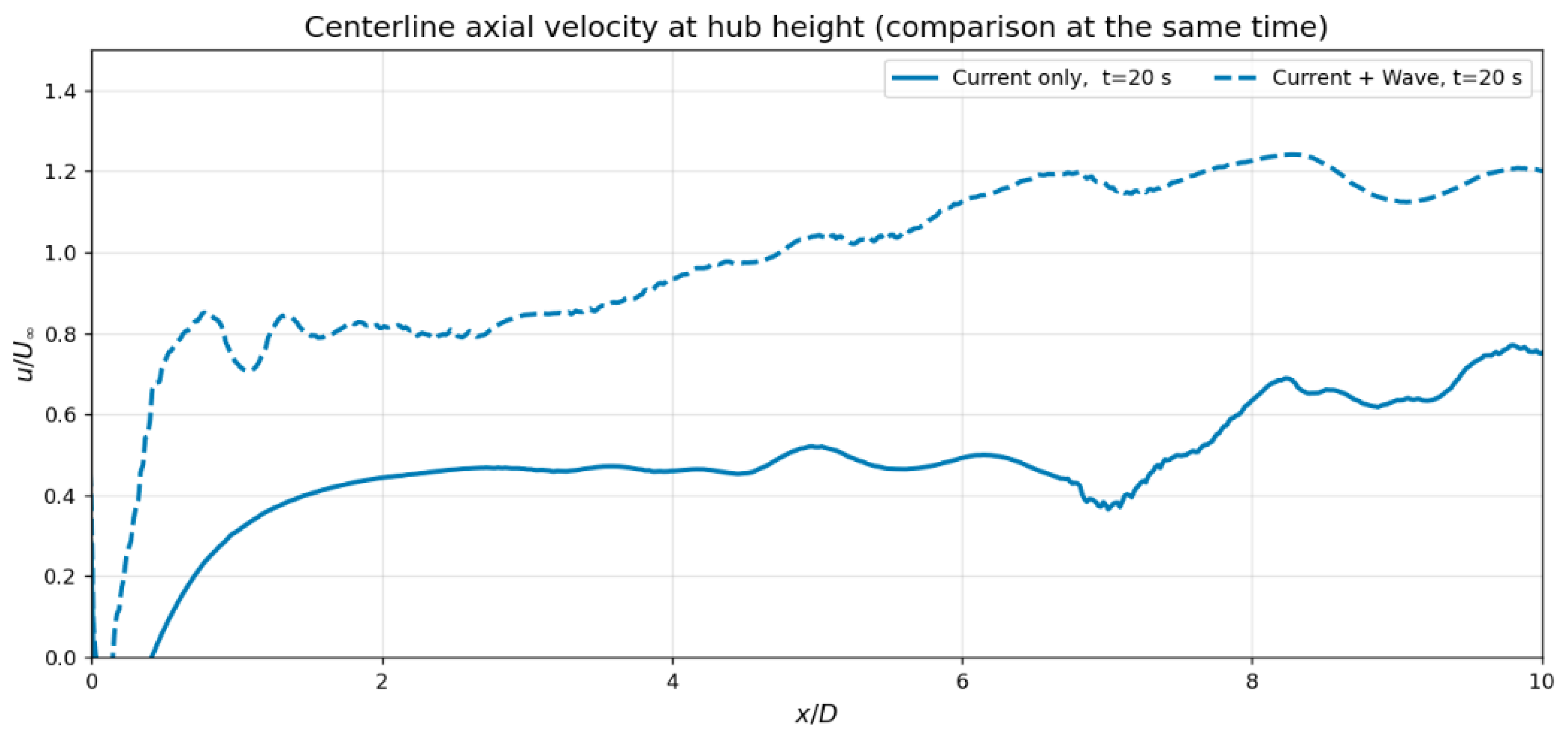
X-directional wake-flow velocity is also plotted for the centerline of the rotor, which is shown in Figure 16. The wave forcing noticeably accelerates wake recovery. The dashed curve rises sooner and overshoots the freestream, reaching $u/U_{\infty }\approx 1.25$–$1.30$ by $x/D\approx 7$–8, whereas the current–only wake approaches $u/U_{\infty }\approx 0.75$–$0.8$ over the same range. Overall, waves shorten the near-wake and enhance momentum re-entry along the centerline, which yields a shallower and faster-recovering wake.

Figure 16. Centerline axial velocity at hub height, normalized by the inflow, comparing the current–only case (solid) and the current + wave case (dashed) at $t=20$ s. (for TSR = 3.6).

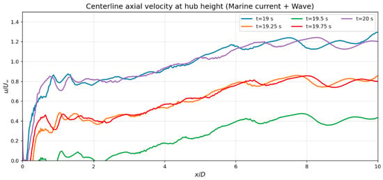
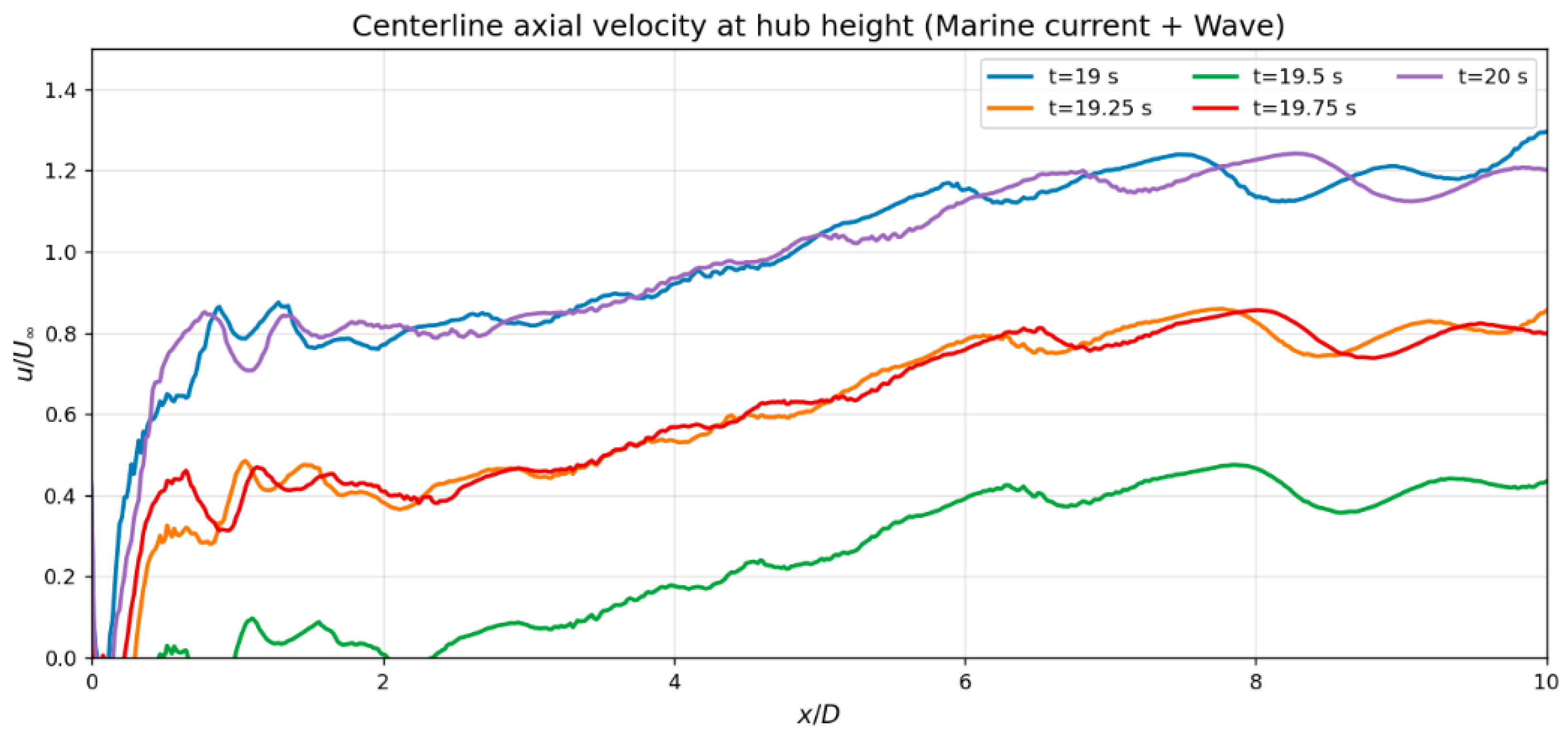
Figure 17 highlights how the wake responds to the instantaneous wave phase. When the wave imposes a favourable pressure gradient (e.g., $t=19$ s and $t=20$ s, blue and purple), the wake recovers rapidly and even overshoots the freestream, reaching $u/U_{\infty }\approx 1.25$–$1.3$ by $x/D\sim 7$–8. Intermediate phases ($t=19.25$ s and $t=19.75$ s, orange and red) yield a milder recovery that asymptotes near $u/U_{\infty }\approx 0.9$. The adverse phase ($t=19.5$ s, green) produces the deepest and longest deficit, with the centerline remaining below $u/U_{\infty }\approx 0.5$ far downstream. In general, the wave modulates the wake by periodically accelerating or decelerating the inflow at the rotor, shortening the near-wake and causing overspeed during favorable phases, and deepening/delaying recovery during adverse phases.

Figure 17. Centerline axial velocity at hub height for the current + wave case over one wave period. Curves show $u/U_{\infty }$ sampled along the centerline ($z\approx 0$) as a function of $x/D$ at $t=\{19,19.25,19.5,19.75,20\}$ s. (for TSR = 3.6).

Overall, these results indicate that wave-induced velocity oscillations modify the near-wake structure and delay wake recovery compared to current-only conditions. From a design perspective, this suggests that turbine spacing and array layout based solely on steady-current assumptions may underestimate wake persistence in wave-active environments. The observed differences highlight the need to account for wave–current interactions when assessing turbine performance and downstream loading.

5.3. Temporal Evolution of Sea Bed

5.3.1. Under the Turbine

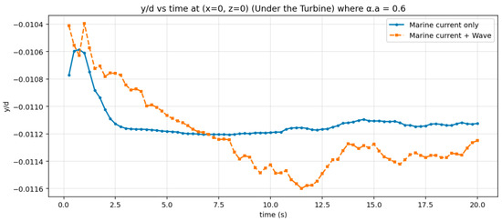
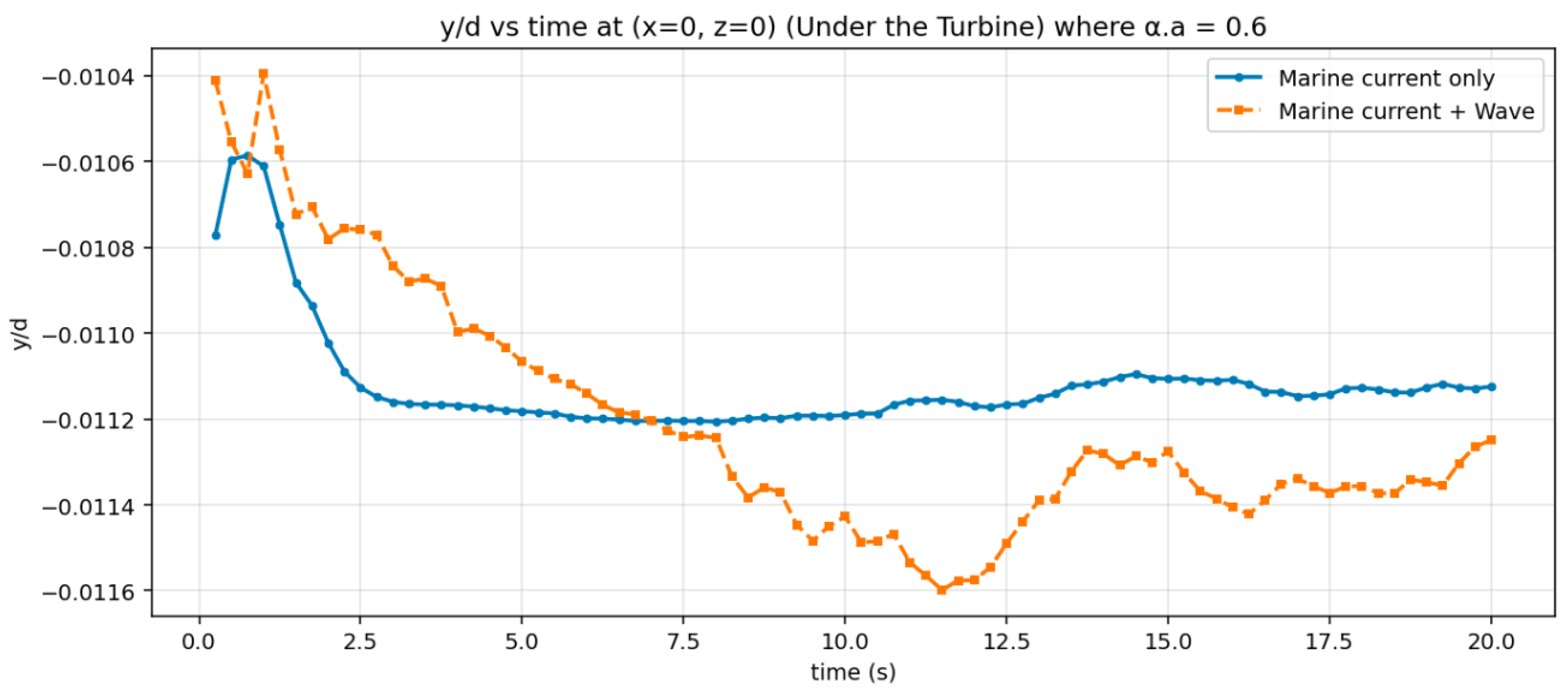
Figure 18 illustrates the temporal evolution of bed elevation ($y/d$) beneath the turbine for a tip-speed ratio (TSR) of 3.6. In this case, we observe that the erosion under the turbine in the presence of a marine current (represented by the blue line) follows a linear pattern after 2.5 s, whereas, in the scenario with both a marine current and wave conditions, there are alternating phases of erosion and deposition. Overall, the absolute scour magnitude and the rate of scour development at a TSR of 3.6 are quite slow.

Figure 18. Comparison of Normalized bed elevation ($y/d$) for current & current + wave (under the turbine) for TSR equal to 3.6.

Deng et al. [44] conducted a similar investigation focusing solely on a turbine scenario that lasted approximately 450 min by using the Volume Of Fluid (VOF) method. The methodological divergence between the present study and the VOF-based approach of Deng et al. [44] stems from a fundamental trade-off between interface resolution and near-bed physical fidelity. While the VOF method excels at tracking the large-scale deformation of the air–water interface, it imposes a severe constraint on the time step to maintain numerical stability at the free surface, often necessitating coarser grid resolutions near the seabed to remain computationally viable over 450-minute durations. In contrast, by employing a rigid-lid approximation with an imposed analytical wave body force, the current framework bypasses interface tracking to prioritize the high-resolution modeling of the two-phase sediment layer. This allows the $SedFoam$ solver to explicitly resolve the $61\%$ concentration sheet-flow regime and the complex inter-phase momentum exchange that drives sediment entrainment. Consequently, while Deng et al. [44] provide a valuable estimate of the long-term equilibrium scour depth ($S/D=0.2$), our 20-cycle simulation offers a high-fidelity ’mechanistic snapshot’ of the phase-locked scouring initiation that acts as the precursor to such long-term morphological changes.

The simulations were rerun for the case where the tip-speed Ratio (TSR) is equal to 5. The results can be seen in Figure 19, which illustrates the scouring evolution under the turbine over a period of 20 s. In the case of the marine current, erosion occurs until the 10-s mark, after which it becomes linear. Conversely, in the current-wave scenario, erosion takes place for the first 12 s, followed by deposition, indicating that wave-induced oscillations significantly influence bed evolution.

Figure 19. Comparison of Normalized Bed Elevation ($y/d$) for Current and Current + Wave (Under the Turbine) for TSR equal to 5.

Figure 20 depicts the temporal evolution of bed elevation ($y/d$) under the turbine for the case of TSR equal to 9. During the initial observations (around 17 s), the formation of scour is showing almost the same pattern for both the current and current-wave case. By the 20-s mark, scour depths increase significantly under combined wave–current conditions, clearly highlighting the rapid sediment mobilization and morphological changes caused by wave-induced processes.

Figure 20. Comparison of Normalized Bed Elevation ($y/d$) for Current and Current + Wave (Under the Turbine) for TSR equal to 9.

By comparing Figure 18, Figure 19 and Figure 20, it is evident that erosion is significantly more pronounced in the case of high TSR (equal to 9) compared to low TSR (equal to 3.60). This increased erosion is attributed to the much stronger tip vortices generated during high TSR conditions, which rapidly cause erosion under the turbine.

5.3.2. 1.16d Downstream of the Turbine

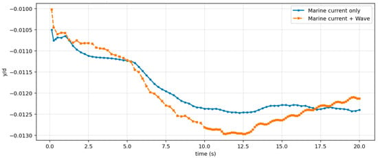
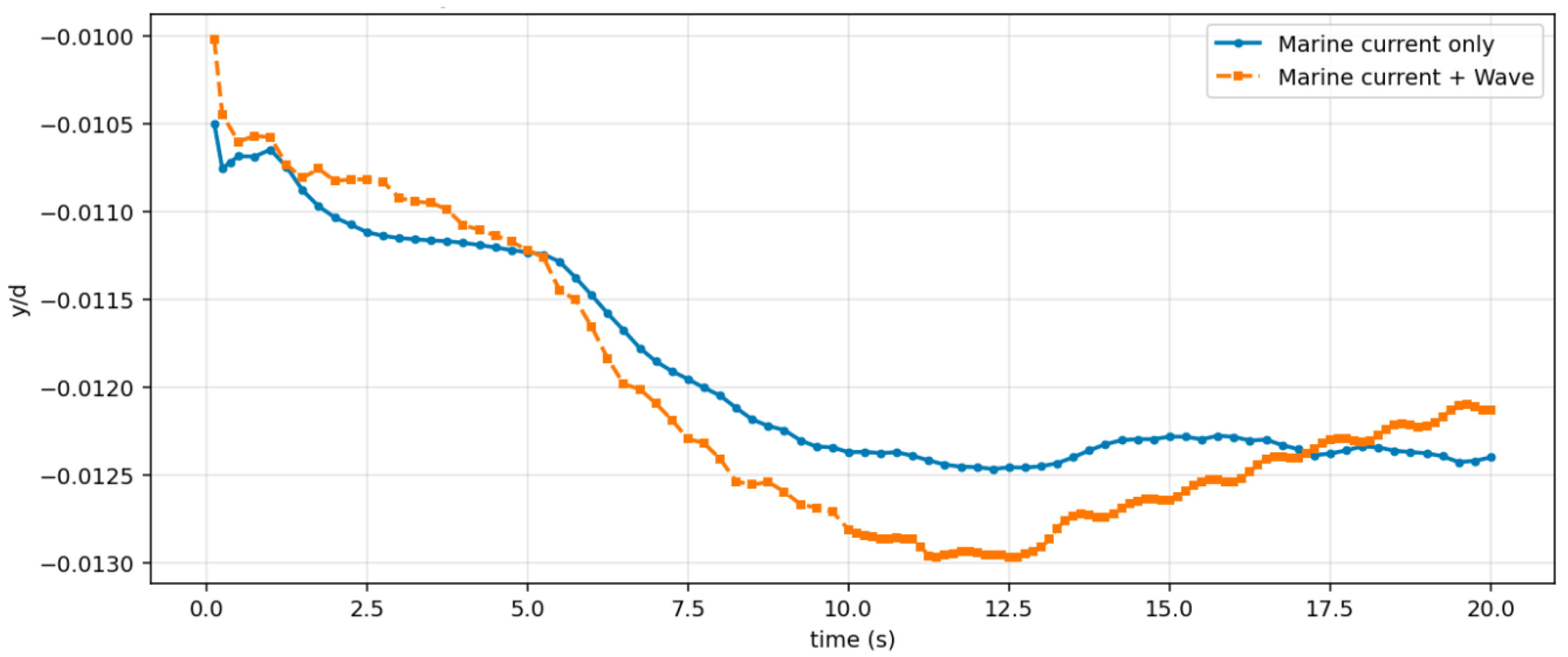
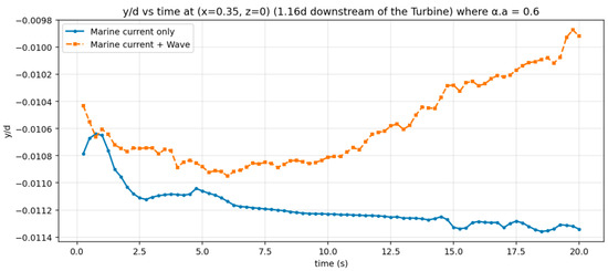
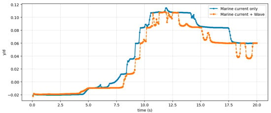
Figure 21 illustrates the temporal evolution of the normalized bed elevation ($y/d$) measured at a location 1.16 turbine diameters downstream of the rotor for a tip-speed ratio (TSR) of 3.6. In the case of combined current and wave conditions, we observe that deposition occurs, with the bed elevation oscillating between erosion and deposition, though the net effect is deposition. In contrast, under current-only conditions, erosion takes place very slowly until approximately 20 s.

Figure 21. Temporal variation of normalized bed elevation ($y/d$) 1.16d downstream of the turbine, comparing current-only and combined current-wave scenarios for TSR equal to 3.6.

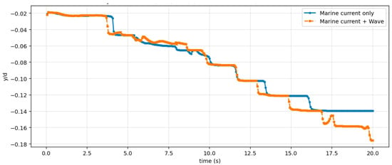
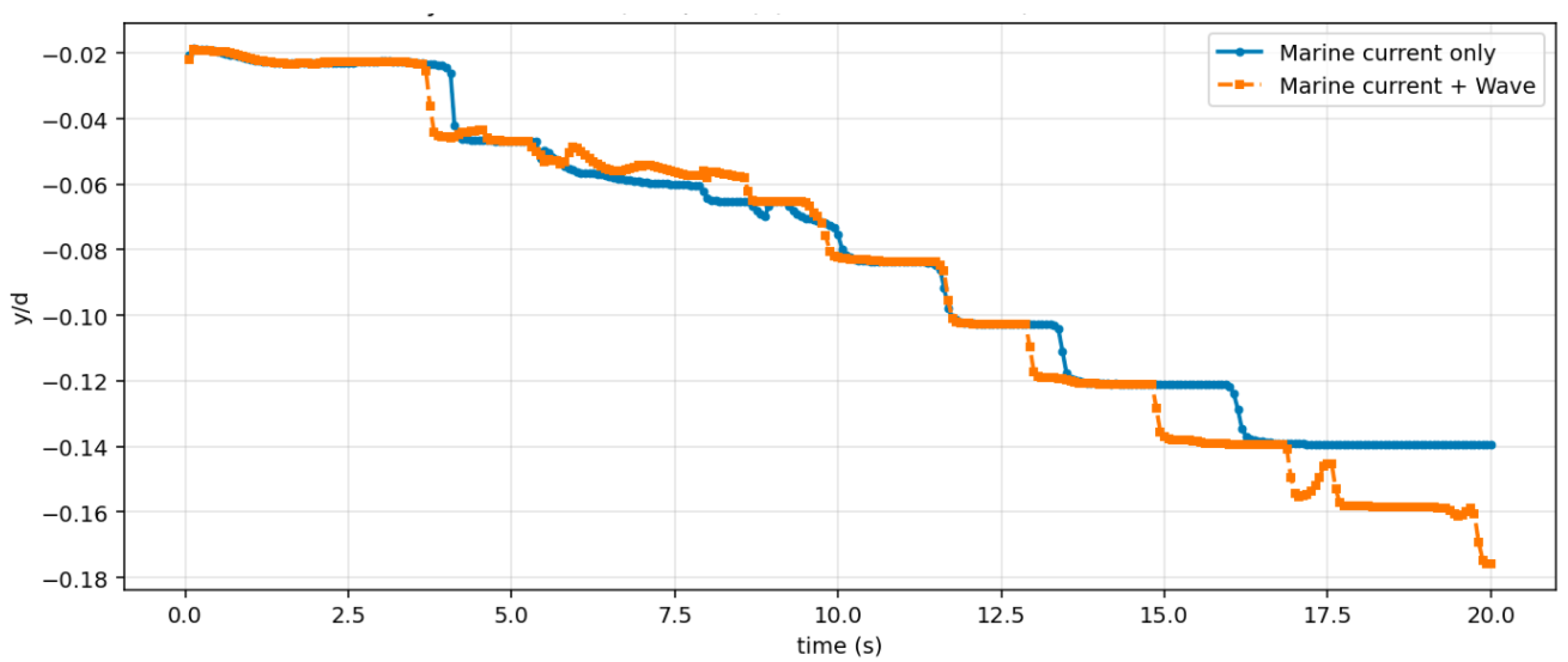
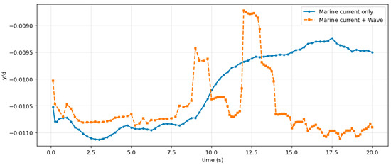
Figure 22 shows the temporal evolution of the normalized bed elevation ($y/d$) measured at a location 1.16 turbine diameters downstream of the rotor, specifically for a tip-speed ratio (TSR) of 5. In contrast, Figure 23 presents the same data for a TSR of 9. Both figures compare the evolution of the sediment bed under current-only conditions with combined wave–current conditions. The results suggest that when waves are present, the sediment bed shows significant oscillatory behavior due to the periodic motion of the waves. The oscillations in bed elevation indicate cycles of sediment resuspension and redeposition caused by wave action. In contrast, under conditions with only current, the bed elevation maintains a relatively steady and smooth profile, with smaller fluctuations in magnitude. Overall, in the case of a high tip-speed ratio (TSR) of 9, deposition occurs at a faster rate compared to a low TSR of 3.6.

Figure 22. Temporal variation of normalized bed elevation ($y/d$) 1.16d downstream of the turbine, comparing current-only and combined current-wave scenarios for TSR equal to 5.

Figure 23. Temporal variation of normalized bed elevation ($y/d$) 1.16d downstream of the turbine, comparing current-only and combined current-wave scenarios for TSR equal to 9.

5.4. Morphodynamic Impact of the Turbine

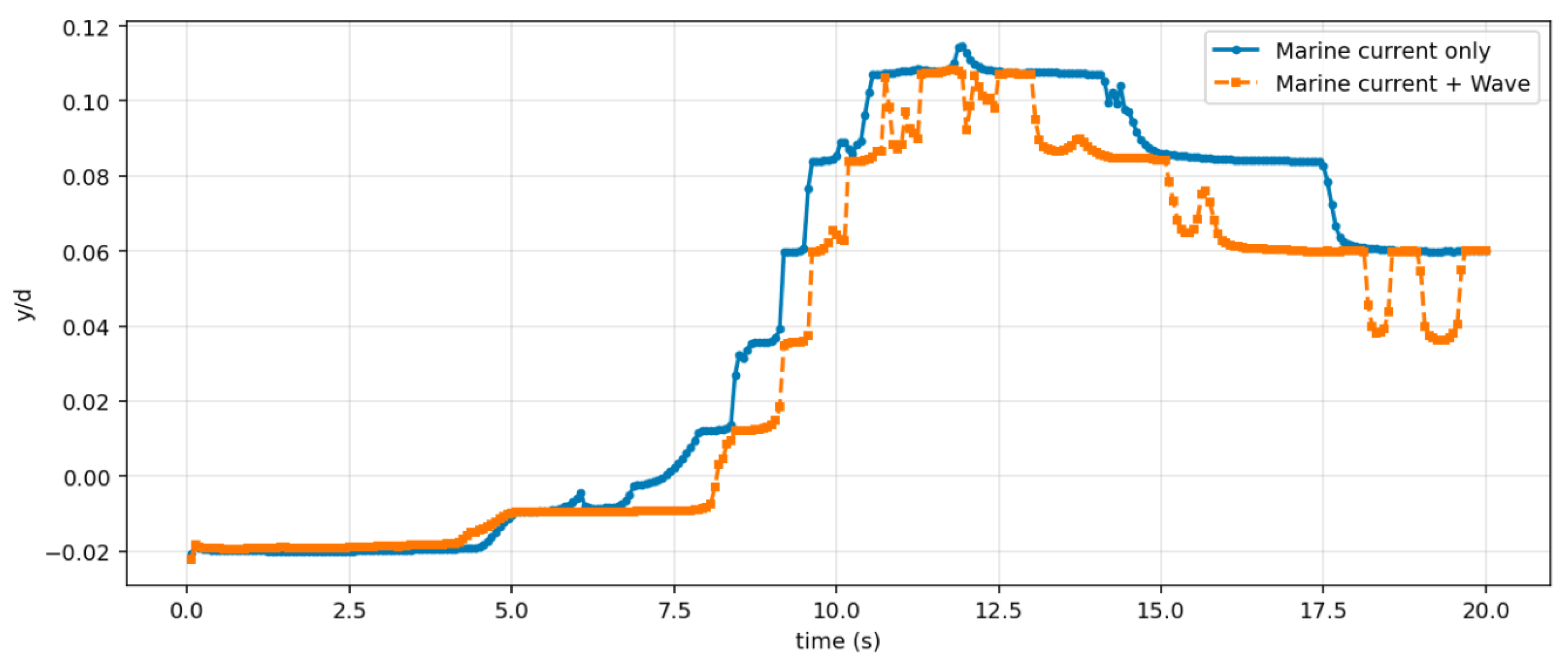
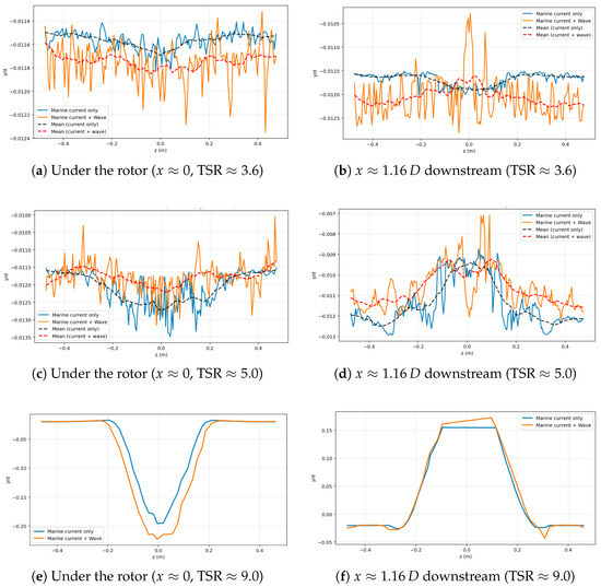
Figure 24 shows spanwise profiles of normalized bed elevation $y/d$ at $t=20$ s for two cases —marine current only and marine current + wave— sampled under the rotor ($x\approx 0$) and $1.16d$ downstream. The thin solid lines are the instantaneous profiles, and the dashed curves indicate the spanwise mean trend.

Figure 24. Spanwise cross-sections of normalized bed elevation ($y/d$) at $t=20$ s. Blue: marine current only; orange: marine current + wave. Each row corresponds to a tip-speed ratio (TSR = 3.6, 5.0, 9.0). Left column: under the rotor ($x\approx 0$). Right column: $x\approx 1.16D$ downstream. Thin lines are instantaneous profiles; dashed lines are spanwise means that highlight the erosion/deposition structure.

At $\mathrm{TSR}\approx 3.6$, the response of the bed is weak (Figure 24a,b). In the case of waves the erosion is increased under the turbine, while later in the downstream, there is deposition taking place at a distance of 1.16d. This shows that the position of deposition is changed due to the effect of waves.

For the moderate $\mathrm{TSR}\approx 5.0$, a symmetric scour bowl begins to form beneath the rotor (Figure 24c). Here, the mean scour is shallower for the wave–current case, suggesting that oscillatory motions refill the erosion area, and overall, the erosion is less under the turbine. But still near the lateral walls, the total erosion is still greater than the case of the current only case. At 1.16d downstream of the turbine (Figure 24d), the overall deposition is greater in the case of the current + wave case, which shows a net deposition at this section.

At the highest $\mathrm{TSR}\approx 9.0$, a symmetric scour bowl develops under the turbine and is significantly deepened by the wave–current forcing (Figure 24e). By $x\approx 1.16D$ (Figure 24f), the profiles evolve into a broad depositional platform; waves slightly increase the top level consistent with enhanced bed mobility. Overall, increasing TSR amplifies the erosion–deposition pattern and significantly affects the overall cross-section pattern at different locations.

It is important to note that the spanwise bed elevation profiles shown in Figure 24 may be influenced by the lateral symmetry conditions. These conditions can artificially constrain the lateral spreading of the turbulent wake and the subsequent dispersion of suspended sediment. While the rotor-centered scour bowl is well-captured, the lateral ’wings’ of the deposition zones might be more confined compared to an open-sea environment where lateral wake meandering is fully realized. Nevertheless, for the short morphodynamic timescales considered here, the symmetry condition provides a reliable estimate of the primary erosion-deposition footprint.

The observed intensification of the scour-deposition pattern under wave–current conditions is consistent with experimental findings in laboratory settings. Physical model studies on structural stability in sandy beds, such as those by Khan-Mozahedy et al. [45], have demonstrated that wave-induced pressure gradients can lead to significant bed liquefaction and structural sinking, effectively accelerating the morphodynamic response. In our simulations, the oscillatory shear stress from the waves serves as a catalyst for sediment entrainment, where rotor-induced turbulence and wave–current interactions combine to deepen the erosion minimum.

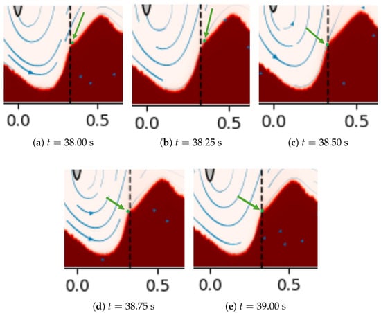
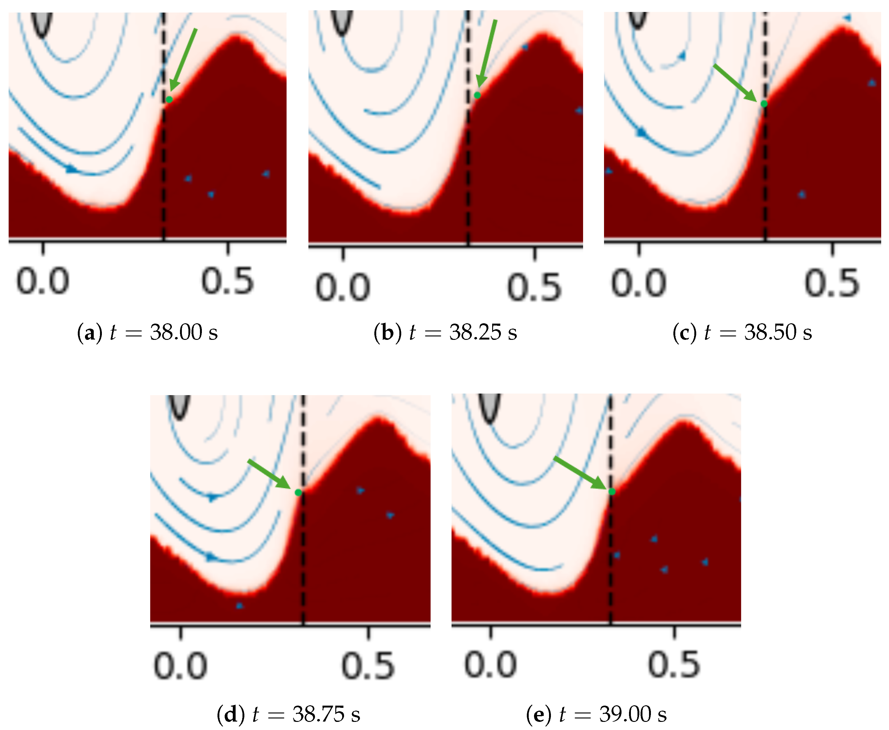
We can observe the effect of the oscillation on the mobility of the sediment in Figure 25. The green dot represents the top mobile sediment particle, which is influenced by the oscillatory motion caused by the wave. The dashed line indicates the reference location, set at 0.33 m. In this case, the wave period is one second. At 38 s, the sediment particle is positioned to the right of the reference line. After some time, it moves even further to the right, as shown in Figure 25b. By 38.5 s, the particle starts to move back toward the reference line, and at 38.75 s, it shifts toward the left extreme. Ultimately, at the end of the phase, the particle returns to the reference line. This demonstrates that sediment particles are continuously influenced by the wave. It’s important to note that the particle’s returning position at the end of the phase may differ from its initial position at the start. This discrepancy is due to the overall stream velocity and the friction between sediment particles, which also impact their movement.

Figure 25. Phase-resolved snapshots of the near-bed region showing the evolution of the flow over the sediment bump (dashed vertical line marks the reference location at x = 0.3). Times progress from $t=38.00$ to $39.00$ s (TSR = 9). The pictures show the region of x = −0.05 to 0.6 and y = −0.14 to 0.15.

5.5. Impact of the Turbine on the Bottom Topography

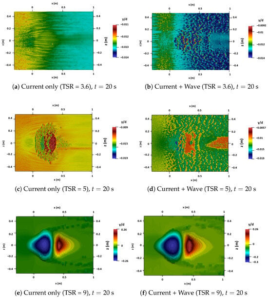
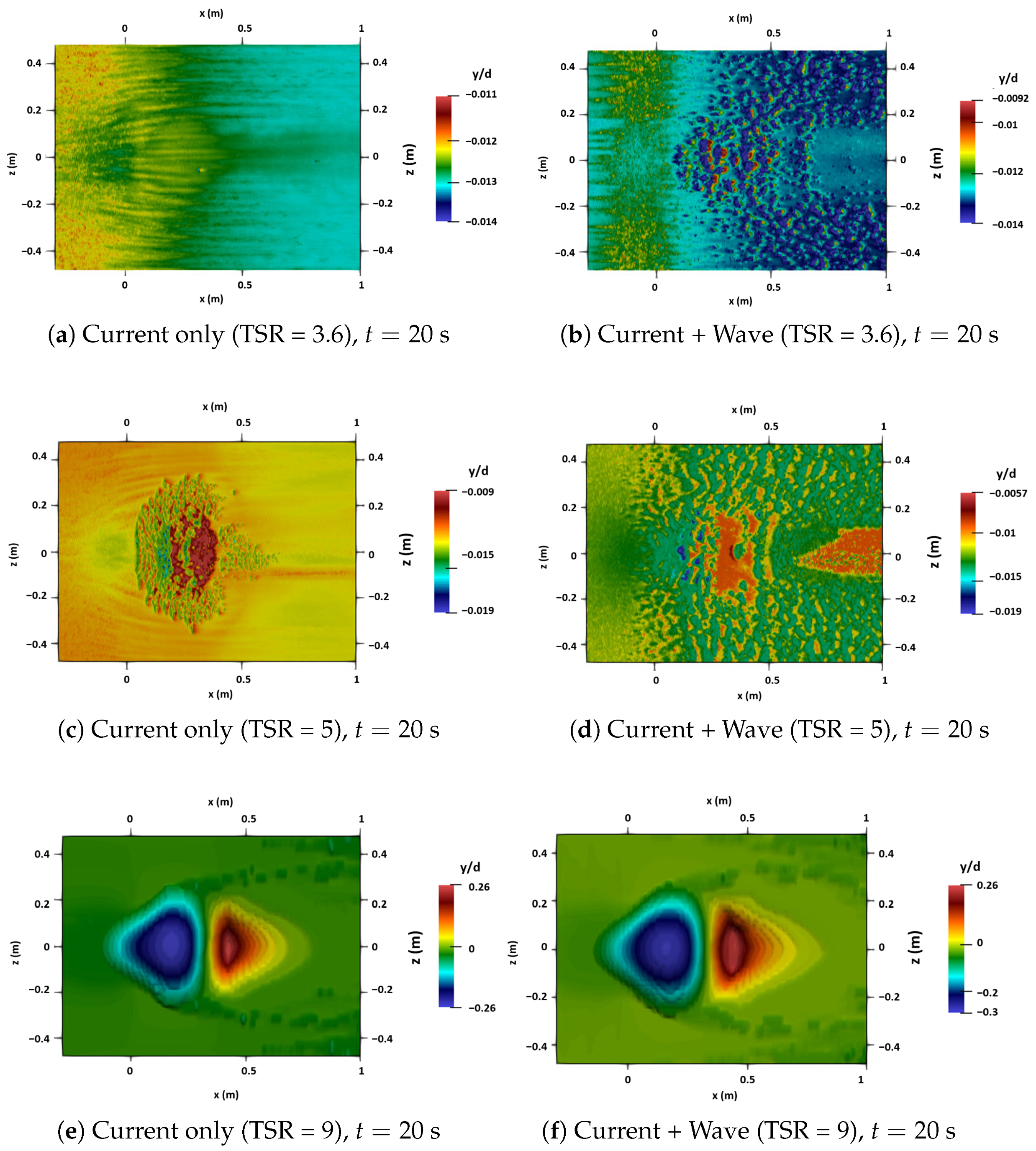
The comparison of simulated bottom topography, expressed as normalized bed elevation ($y/d$), is illustrated in Figure 26. The top row represents a case with a tip-speed ratio (TSR) of 3.6, where the patterns exhibit significant ripple-scale variability, which means that there are high-frequency bed undulations that appear as alternating patches of erosion and deposition, with no persistent, rotor-centered depression. The blue region indicates erosion, while the red region indicates deposition. There is no distinct area of erosion or deposition in the case of TSR equal to 3.6 and 5. In contrast, when the tip-speed ratio is set to 9, a clear pattern of scour and deposition emerges. We identify a coherent scour response when the spanwise-averaged bed profile exhibits a clear, smooth trend with a distinct minimum under the rotor and a consistent downstream deposition zone. Compared to the current-only scenario, the combination of wave and current forces broadens the area affected and deepens the minimum erosion point. This enhancement is consistent with the additional oscillatory shear that facilitates sediment mobilization.

Figure 26. Bottom topography (normalized bed elevation $y/d$) in the x–z plane at $t=20$ s captures the state at the wave crest (transient state). Blue indicates erosion ($y/d<0$) and red deposition ($y/d>0$). Top row: marine current only. Bottom row: marine current + wave.

To quantify these patterns, the maximum normalized bed changes were sampled at $t=20$ s. At $TSR=3.6$ and 5, the bed response is dominated by ripple-scale fluctuations with depths around $-1.4\times {10}^{-2}D$ and $-1.9\times {10}^{-2}D$ respectively. In contrast, at the highest $TSR=9$, the coherent scour bowl reaches a maximum depth of $-0.26D$ under current-only conditions. The addition of wave forcing deepens this minimum to $-0.30D$, representing a significant increase in sediment mobilization due to the additional oscillatory shear stress.

5.6. Scope and Limitation

The simulations presented in this study are limited to a total duration of 20 s and, as such, primarily capture the early-time dynamics of the sediment response rather than an equilibrium scour state. The objective is to resolve the coupled interactions between turbine forcing, wave-induced oscillatory motion, and two-phase sediment transport at the device scale. Achieving this requires small time steps and high spatial resolution to ensure numerical stability, particularly in dense near-bed regions where sediment transport is most sensitive to hydrodynamic forcing.

In the present setup, the imposed wave period is $T=1$ s, such that a 20 s simulation spans 20 complete wave cycles. This time window is sufficient to capture repeatable, phase-dependent modulation of the flow field and the associated oscillatory erosion–deposition response of the seabed over short timescales. Accordingly, the results are intended to describe short-term trends in scour initiation and near-wake-driven bed adjustment under current-only and wave–current forcing, rather than final or equilibrium scour depths.

With respect to wave physics, waves are imposed using first-order wave theory through a time-varying body force and modified inlet boundary conditions. This representation is computationally efficient and reproduces the primary oscillatory forcing (pressure-gradient-driven and velocity-driven fluctuations) superimposed on the mean current; however, it inherently corresponds to regular, linear, sinusoidal wave motion. Although the model can capture phase-dependent modulation of bed response under linear oscillatory forcing, several near-bed processes that can be important for sediment transport are not explicitly represented. We also note that the wave–current bottom boundary layer mechanisms often described by Grant–Madsen-type formulations are not explicitly verified in the present work. Addressing these aspects would require additional diagnostics and/or dedicated near-bed experimental measurements for the same configuration, which are beyond the scope of the current study.

Finally, equilibrium scour and large-scale bedform adjustment typically occur over much longer timescales (hours to days, or multiple tidal cycles). Capturing these processes would require substantially longer simulations or morphodynamic acceleration techniques, which are outside the scope of the current work. Therefore, the conclusions regarding net scouring and long-term morphodynamic impacts should be interpreted as preliminary insights into early-stage seabed evolution. Future work will consider longer-duration simulations and additional near-bed validation metrics to better quantify wave–current boundary-layer effects on sediment transport.

6. Conclusions

This study extended the three-dimensional two-phase solver SedFoam-2.0 to simulate the coupled interaction of surface waves, tidal currents, and a turbine rotor over a mobile sediment bed. The turbine was represented through a Blade Element Theory (BET) momentum source, while the wave forcing was imposed through a first-order wave theory (FOWT) body force and modified inlet boundary conditions. The numerical implementation was validated in a two-stage process: first, the BET method accurately reproduced the wake statistics and axial velocity deficits from laboratory experiments, and second, the wave module matched analytical solutions for wave–current average flow velocity.

The main findings of this research highlight the complex interactions between hydrodynamic forcing and seabed morphology. Regarding wake dynamics under combined wave–current forcing, the centerline velocity exhibits significant overshoots during favorable wave phases and deeper deficits during adverse phases; however, these phase-induced effects decay rapidly beyond approximately 4 D as turbulent mixing redistributes momentum back into the wake. While the rigid-lid approximation and the first-order wave theory represent a simplification of the shallow water approximation, this framework allows the high-fidelity resolution of the two-phase sediment layer and the rotor-wake interaction within a manageable computational budget.

From a morphodynamic perspective, the presence of waves enhances near-bed shear stress and sediment mobility, resulting in amplified scour under the rotor compared to current-only conditions. Furthermore, the bed elevation downstream of the turbine oscillates in synchronization with the wave period. It was observed that a higher tip-speed ratio (TSR) strengthens tip-vortex-driven shear, which accelerates both the scouring process beneath the rotor and the subsequent sediment deposition. In terms of the spatial footprint, wave–current forcing broadens the region of significant bed change and deepens the erosion minimum beneath the turbine when compared to current-only scenarios. While the bed response is weaker and dominated by ripple-scale variability at lower TSR values, a coherent and distinct scour-deposition pattern emerges at higher TSRs.

These findings suggest that neglecting wave–current interactions may lead to biased predictions of wake recovery and local scour, which have direct implications for turbine spacing and the conservative design of foundations in wave-active estuarine environments. Future work will focus on a comprehensive sensitivity analysis of the empirical rheological constants to further establish the robustness of these morphodynamic predictions across various sediment types. Additionally, the framework can be extended to investigate long-term bedform evolution using morphodynamic acceleration techniques and to incorporate structural components, such as turbine support piles, which may further influence sediment dynamics in combined wave–current regimes. Furthermore, the integration of higher-order or irregular wave theories would allow for a more realistic representation of the nonlinear wave–current interactions prevalent in shallow estuarine sites.

References

- Newell, R.; Raimi, D.; Aldana, G. Global energy outlook 2019: The next generation of energy. Resour. Future 2019, 1, 1–37. [Google Scholar]
- Neill, S.P.; Hashemi, M.R. Fundamentals of Ocean Renewable Energy: Generating Electricity from the Sea; Academic Press: Cambridge, MA, USA, 2018. [Google Scholar]
- Filonchyk, M.; Peterson, M.P.; Zhang, L.; Hurynovich, V.; He, Y. Greenhouse gases emissions and global climate change: Examining the influence of CO2, CH4, and N2O. Sci. Total Environ. 2024, 935, 173359. [Google Scholar] [CrossRef] [Scilit]
- Wang, J.; Azam, W. Natural resource scarcity, fossil fuel energy consumption, and total greenhouse gas emissions in top emitting countries. Geosci. Front. 2024, 15, 101757. [Google Scholar] [CrossRef] [Scilit]
- Kazimierczuk, K.; Henderson, C.; Duffy, K.; Hanif, S.; Bhattacharya, S.; Biswas, S.; Jacroux, E.; Preziuso, D.; Wu, D.; Bhatnagar, D.; et al. A socio-technical assessment of marine renewable energy potential in coastal communities. Energy Res. Soc. Sci. 2023, 100, 103098. [Google Scholar] [CrossRef] [Scilit]
- Lago, L.; Ponta, F.; Chen, L. Advances and trends in hydrokinetic turbine systems. Energy Sustain. Dev. 2010, 14, 287–296. [Google Scholar] [CrossRef] [Scilit]
- Khan, M.; Bhuyan, G.; Iqbal, M.; Quaicoe, J. Hydrokinetic energy conversion systems and assessment of horizontal and vertical axis turbines for river and tidal applications: A technology status review. Appl. Energy 2009, 86, 1823–1835. [Google Scholar] [CrossRef] [Scilit]
- Yuce, M.I.; Muratoglu, A. Hydrokinetic energy conversion systems: A technology status review. Renew. Sustain. Energy Rev. 2015, 43, 72–82. [Google Scholar] [CrossRef] [Scilit]
- Ramírez-Mendoza, R.; Amoudry, L.; Thorne, P.; Cooke, R.; McLelland, S.; Jordan, L.; Simmons, S.; Parsons, D.; Murdoch, L. Laboratory study on the effects of hydro kinetic turbines on hydrodynamics and sediment dynamics. Renew. Energy 2018, 129, 271–284. [Google Scholar] [CrossRef] [Scilit]
- Neill, S.P.; Litt, E.J.; Couch, S.J.; Davies, A.G. The impact of tidal stream turbines on large-scale sediment dynamics. Renew. Energy 2009, 34, 2803–2812. [Google Scholar] [CrossRef] [Scilit]
- Nikitas, G. A Study on Soil-Structure Interaction of Offshore Wind Turbine Foundations. Ph.D. Thesis, University of Surrey, Guildford, UK, 2020. [Google Scholar]
- Hauer, C.; Leitner, P.; Unfer, G.; Pulg, U.; Habersack, H.; Graf, W. The role of sediment and sediment dynamics in the aquatic environment. In Riverine Ecosystem Management: Science for Governing Towards a Sustainable Future; Springer International Publishing: Cham, Switzerland, 2018; pp. 151–169. [Google Scholar]
- Ribbe, J.; Holloway, P.E. A model of suspended sediment transport by internal tides. Cont. Shelf Res. 2001, 21, 395–422. [Google Scholar] [CrossRef] [Scilit]
- Mathieu, A. Development of the Two-Fluid Turbulence-Resolving Approach for Sediment Transport Applications. Ph.D. Thesis, Université Grenoble Alpes, Saint-Martin-d’Hères, France, 2021. [Google Scholar]
- Van Rijn, L.C. Unified view of sediment transport by currents and waves. I: Initiation of motion, bed roughness, and bed-load transport. J. Hydraul. Eng. 2007, 133, 649–667. [Google Scholar] [CrossRef] [Scilit]
- Grant, W.D.; Madsen, O.S. Combined wave and current interaction with a rough bottom. J. Geophys. Res. Ocean. 1979, 84, 1797–1808. [Google Scholar] [CrossRef] [Scilit]
- Soulsby, R.L.; Damgaard, J.S. Bedload sediment transport in coastal waters. Coast. Eng. 2005, 52, 673–689. [Google Scholar] [CrossRef] [Scilit]
- Fredsoe, J.; Deigaard, R. Mechanics of Coastal Sediment Transport; World Scientific: Singapore, 1992; Volume 3. [Google Scholar]
- Liu, L.; Franceschini, L.; Oliveira, D.F.; Galeazzo, F.C.; Carmo, B.S.; Stevens, R.J. Evaluating the accuracy of the actuator line model against blade element momentum theory in uniform inflow. Wind Energy 2022, 25, 1046–1059. [Google Scholar] [CrossRef] [Scilit]
- Batten, W.; Bahaj, A.; Molland, A.; Chaplin, J. The prediction of the hydrodynamic performance of marine current turbines. Renew. Energy 2008, 33, 1085–1096. [Google Scholar] [CrossRef] [Scilit]
- Churchfield, M.J.; Li, Y.; Moriarty, P.J. A large-eddy simulation study of wake propagation and power production in an array of tidal-current turbines. Philos. Trans. R. Soc. A Math. Phys. Eng. Sci. 2013, 371, 20120421. [Google Scholar] [CrossRef] [Scilit]
- Mycek, P.; Gaurier, B.; Germain, G.; Pinon, G.; Rivoalen, E. Experimental study of the turbulence intensity effects on marine current turbines behaviour. Part I: One single turbine. Renew. Energy 2014, 66, 729–746. [Google Scholar] [CrossRef] [Scilit]
- Mason-Jones, A. Performance Assessment of a Horizontal Axis Tidal Turbine in a High Velocity Shear Environment; Cardiff University: Cardiff, UK, 2010. [Google Scholar]
- Draycott, S.; Steynor, J.; Nambiar, A.; Sellar, B.; Venugopal, V. Experimental assessment of tidal turbine loading from irregular waves over a tidal cycle. J. Ocean Eng. Mar. Energy 2019, 5, 173–187. [Google Scholar] [CrossRef] [Scilit]
- Li, Q.; Venugopal, V.; Barltrop, N. Modelling dynamic loadings of a tidal stream turbine in combined wave-current-turbulence environment. Sustain. Energy Technol. Assess. 2022, 50, 101795. [Google Scholar] [CrossRef] [Scilit]
- Gao, J.; Ma, X.; Dong, G.; Chen, H.; Liu, Q.; Zang, J. Investigation on the effects of Bragg reflection on harbor oscillations. Coast. Eng. 2021, 170, 103977. [Google Scholar] [CrossRef] [Scilit]
- Gao, J.; Ma, X.; Zang, J.; Dong, G.; Ma, X.; Zhu, Y.; Zhou, L. Numerical investigation of harbor oscillations induced by focused transient wave groups. Coast. Eng. 2020, 158, 103670. [Google Scholar] [CrossRef] [Scilit]
- Gao, J.; Hou, L.; Liu, Y.; Shi, H. Influences of bragg reflection on harbor resonance triggered by irregular wave groups. Ocean Eng. 2024, 305, 117941. [Google Scholar] [CrossRef] [Scilit]
- Gao, J.; Wu, Y.; Song, Z.; He, M. Influences of low velocity uniform current on characteristics of gap resonance occurring between two adjacent fixed bodies. Mar. Struct. 2026, 106, 103961. [Google Scholar] [CrossRef] [Scilit]
- Brakenhoff, L.; Schrijvershof, R.; van der Werf, J.; Grasmeijer, B.; Ruessink, G.; van der Vegt, M. From ripples to large-scale sand transport: The effects of bedform-related roughness on hydrodynamics and sediment transport patterns in delft3d. J. Mar. Sci. Eng. 2020, 8, 892. [Google Scholar] [CrossRef] [Scilit]
- Maerker, C.; Malcherek, A.; Riemann, J.; Brudy-Zippelius, T. Modelling and analyzing dredging and disposal activities using Telemac, Sisyphe and DredgeSim. XVIIIth Telemac Mascaret User Club 2011, 19, 92. [Google Scholar]
- Bolle, A.; Mercelis, P.; Roelvink, D.; Haerens, P.; Trouw, K. Application and validation of XBeach for three different field sites. Coast. Eng. Proc. 2011, 1, 40. [Google Scholar] [CrossRef] [Scilit]
- Chauchat, J.; Cheng, Z.; Nagel, T.; Bonamy, C.; Hsu, T.J. SedFoam-2.0: A 3-D two-phase flow numerical model for sediment transport. Geosci. Model Dev. 2017, 10, 4367–4392. [Google Scholar] [CrossRef] [Scilit]
- Hsu, T.J.; Jenkins, J.T.; Liu, P.L.F. On two-phase sediment transport: Sheet flow of massive particles. Proc. R. Soc. Lond. Ser. A Math. Phys. Eng. Sci. 2004, 460, 2223–2250. [Google Scholar] [CrossRef] [Scilit]
- Schiller, L.; Naumann, A. Über die grundlegenden Berechnungen bei der Schwerkraftaufbereitung. Z. Ver. Dtsch. Ing. 1933, 77, 318–320. [Google Scholar]
- Cheng, Z.; Hsu, T.J.; Calantoni, J. SedFoam: A multi-dimensional Eulerian two-phase model for sediment transport and its application to momentary bed failure. Coast. Eng. 2017, 119, 32–50. [Google Scholar] [CrossRef] [Scilit]
- Johnson, P.C.; Jackson, R. Frictional–collisional constitutive relations for granular materials, with application to plane shearing. J. Fluid Mech. 1987, 176, 67–93. [Google Scholar] [CrossRef] [Scilit]
- Chauchat, J.; Médale, M. A three-dimensional numerical model for dense granular flows based on the μ (I) rheology. J. Comput. Phys. 2014, 256, 696–712. [Google Scholar] [CrossRef] [Scilit]
- Khaled, F.; Guillou, S.; Méar, Y.; Hadri, F. Numerical investigation of the local impact of hydrokinetic turbine on sediment transport—Comparison between two actuator models. Eur. J. Mech.-B/Fluids 2023, 102, 31–45. [Google Scholar] [CrossRef] [Scilit]
- Khaled, F.; Guillou, S.; Méar, Y.; Hadri, F. Impact of the blockage ratio on the transport of sediment in the presence of a hydrokinetic turbine: Numerical modeling of the interaction sediment and turbine. Int. J. Sediment Res. 2021, 36, 696–710. [Google Scholar] [CrossRef] [Scilit]
- Khaled, F. Modelization of the Interactions Between Turbine and Sediment Transport, Using the Blade Element Momentum Theory. Ph.D. Thesis, Normandie Université, Caen, France, 2021. [Google Scholar]
- Kundu, P.K.; Cohen, I.M. Fluid Mechanics; Elsevier Academic Press: Cambridge, MA, USA, 2004. [Google Scholar]
- Geuzaine, C.; Remacle, J.F. Gmsh: A 3D Finite Element Mesh Generator with Built-In Pre- and Post-Processing Facilities. Int. J. Numer. Methods Eng. 2009, 79, 1309–1331. [Google Scholar] [CrossRef] [Scilit]
- Deng, X.; Law, A.W.K.; Zhang, J.; Lin, X. Two phase fluid-actuator line-immersed boundary coupling for tidal stream turbine modeling with scouring morphology under wave-current loading. Energy 2025, 329, 136757. [Google Scholar] [CrossRef] [Scilit]
- Khan-Mozahedy, A.; Muñoz-Perez, J.J.; Neves, M.G.; Sancho, F.; Cavique, R. Mechanics of the scouring and sinking of submerged structures in a mobile bed: A physical model study. Coast. Eng. 2016, 110, 50–63. [Google Scholar] [CrossRef] [Scilit]
Disclaimer/Publisher’s Note: The statements, opinions and data contained in all publications are solely those of the individual author(s) and contributor(s) and not of MDPI and/or the editor(s). MDPI and/or the editor(s) disclaim responsibility for any injury to people or property resulting from any ideas, methods, instructions or products referred to in the content. |
© 2026 by the authors. Licensee MDPI, Basel, Switzerland. This article is an open access article distributed under the terms and conditions of the Creative Commons Attribution (CC BY) license.