


Abstract
Autonomous underwater vehicles (AUVs) are increasingly used in marine exploration and underwater operations, where unexpected thruster faults may hinder mission execution and compromise operational safety. Therefore, efficient and reliable fault diagnosis methods are essential for improving the safety and autonomy of AUV operations. Data-driven fault diagnosis approaches provide an efficient way for detecting thruster faults in autonomous underwater vehicles (AUVs). A typical data-driven method that directly supplies the original AUV dynamic signal sequences into a CNN classifier is adopted as the baseline in this study and is referred to as OriCNN. To further improve the representation of fault-related information in the OriCNN, whose temporal location may vary among finite signal windows, and to enrich the available input channels of the OriCNN, this study proposes a CNN-based fault diagnosis framework integrating multidomain data sequence reconstruction (MDDSR) and data channel extension (DCE). MDDSR constructs alternative representations in the time, frequency, and time–frequency domains to reduce the sensitivity of CNN inputs to variations in the temporal location of fault-related features. DCE employs multiple signal processing techniques to generate enhanced data sequences, treats each sequence as an independent data channel, and optimizes channel arrangements to reduce CNN convergence iteration. Experiments using a prototype AUV in a lake were conducted, in which the thruster faults were software-simulated thrust-loss conditions generated by modifying the thruster control-voltage command. Experimental results show that the proposed MDDSR + CNN effectively mitigated the unstable training behavior observed in OriCNN and the proposed MDDSR + DCE + CNN further reduced the convergence iterations while maintaining robustness against different convolution kernel sizes. These results indicate that the proposed MDDSR + CNN and MDDSR + DCE + CNN frameworks contribute to AUV thruster fault diagnosis and thereby to safer and more autonomous underwater operations.
1. Introduction
The abundant biological and mineral resources in oceans have driven increasing global interest in marine exploration and resource utilization [1]. The exploration and extraction of marine resources require high-performance underwater equipment. Due to their high-precision navigation and autonomous operation capabilities in remote marine areas, AUVs have been widely used in marine oil and gas exploration and development, marine surveys, deep-sea sampling, environmental assessment, submarine cable or pipeline inspection, and other tasks related to marine resource development [2]. Underwater thrusters are typically used as power supply components in AUVs [3,4]. These thrusters are subjected to varying loads and high-performance demands during their operation. Thus, underwater thrusters often develop faults such as blade damage, blade biofouling, blade corrosion and motor stall, as shown in Figure 1.
Figure 1.
AUV thruster structure and representative physical failure modes in practical operation.
The physical failure modes illustrated in Figure 1 represent typical mechanisms that may degrade thruster performance during practical underwater operations. Such failures can cause the actual thrust output to deviate from the expected thrust, potentially hindering mission execution and increasing operational risks [5,6]. Therefore, a software-based fault simulation strategy is commonly adopted, in which the thruster control-voltage command is modified to generate different prescribed operating conditions. This strategy provides a surrogate representation of actuator output degradation rather than a direct reproduction of blade damage, blade biofouling, blade corrosion and motor stall.
Existing fault diagnosis methods for underwater thrusters can be classified into two main categories, namely model-based and model-free diagnosis methods [7,8]. Model-based diagnosis methods involve the establishment of a dynamic model of the examined underwater vehicle or underwater thruster system, following which thruster faults are diagnosed by analyzing the residuals between model output values and corresponding sensor-measured values [9,10]. A dynamic model of an underwater vehicle or underwater thruster system can be established using three types of methods. The first type of method involves the creation of an analytical model of system dynamics on the basis of physical laws. Gan, Dong and Chu [11] proposed a thruster fault diagnosis method based on load feature extraction. They established an analytical model of thruster load torque on the basis of the output load characteristics of thrusters under typical fault patterns. Subsequently, they used a sliding-mode observer, a least-squares method, and a support vector machine algorithm to estimate thruster load torque, identify model parameters, and classify fault patterns. Simulation results indicated that the diagnostic accuracy of the aforementioned method was higher than 95% within 5 s of the thruster fault. Song and He [12] proposed a comprehensive AUV model that describes system dynamics and the influence of environmental disturbances on the AUV model, and they used this model to determine the state of the system. They computed residual signals on the basis of reconstruction errors relative to observations and then used these residual signals to detect thruster faults. Simulation experiments demonstrated the effectiveness of the aforementioned method in detecting actuator faults in several cases. Hu, Wu, Zhou and Zeng [13] proposed a fault detection scheme that combines an extended state observer with an adaptive threshold based on a six-degree-of-freedom model of an underwater vehicle. They calculated diagnostic residuals by using extended state variables, and the adaptive threshold was employed to monitor residual changes. The aforementioned method effectively detected thruster and rudder faults. In the three methods described above, faults are diagnosed on the basis of an analytical model. However, the complexity of marine environments hinders the establishment of accurate analytical models [14,15,16].
The second type of method involves establishing a mapping model based on artificial intelligence technology for mapping input control signals to output system state signals. Zhang, Zhang, Yan, Gao and Yu [17] proposed a fault detection method for the rudder system of an AUV. In their method, singular value decomposition is employed to denoise the original sensor data, and a recurrent neural network is then used to identify parameters of an AUV motion model. An adaptive threshold is used to analyze the prediction error, and the results of threshold analysis are combined with those of qualitative force analysis to diagnose and localize rudder system faults. He, Li, Cao, Li, Jiang and An [10] proposed an improved particle-filter-based prediction method. In this method, gray prediction is conducted to accurately estimate and track the fault state of the examined thruster. Moreover, a Gaussian kernel function is adopted to evaluate the reliability of the prediction results, thereby effectively reducing the possibility of false diagnosis. In the aforementioned two methods, control signals output by a controller and state data measured by sensors are used to establish a system dynamics model, which consequently has relatively high accuracy. However, these methods do not provide a deep explanation of the established model [18,19].
The third type of method involves the integration of an analytical model with a mapping model. Gao, Liu, Zhang, Feng, He and Zio [20] developed a fault detection framework for underwater thrusters by combining a physical model and a generative adversarial network. This framework can integrate physical information into the training of the generative adversarial network and yield a model that accurately detects thruster damage and biofouling faults on the basis of a small number of fault-free samples. Chu, Chen, Zhu and Zhang [21] established a fault detection framework for magnetically coupled underwater thrusters by integrating a sliding-mode observer with a neural network model. This framework uses a recurrent neural network to model underwater thrusters and employs a sliding-mode observer to detect faults. Experimental results indicated the effectiveness of the thruster modeling technique and fault detection method. Although these hybrid frameworks combine analytical and data-driven mapping models, they do not fully overcome the limitations of model-based diagnosis. Accurate analytical models are difficult to establish in complex marine environments, whereas data-driven mapping models provide limited interpretability. Therefore, hybrid model-based approaches remain subject to a trade-off between modeling accuracy and interpretability.
Unlike model-based methods, model-free methods do not involve the establishment of a dynamic model of underwater vehicles or underwater thrusters; rather, they rely on the direct learning of the relationship between the state data of underwater vehicles or thrusters and fault patterns from training data [22,23]. Model-free diagnostic methods are primarily of two types: two-stage and single-stage diagnostic methods.
Two-stage diagnostic methods consist of two stages: feature extraction and fault classification. Cui, Zhang, Zhang and Liu [24] proposed a thruster fault feature extraction method based on resonance sparse signal decomposition a fault severity identification method in which Euclidean distance and gray relations are combined. This method can efficiently determine the severity of thruster faults. Chu, Gu, Li, Chen and Zhang [25] developed a fault diagnosis method based on the combination of particle swarm optimization and a hidden Markov model for underwater thrusters. In their method, a three-step approach is employed for preprocessing thruster data, followed by fault classification using a hidden Markov model optimized with the particle swarm optimization algorithm. Yin, Wang, Zhang, Jin and Liu [26] established a time–frequency energy method based on the smoothed pseudo Wigner–Ville distribution (SPWVD) for feature extraction, they used transferable support vector data description for fault severity classification. Jiang, Feng, He, Guo, Wang and Lv [27] created a fault diagnostic framework by combining a wide convolutional neural network (CNN) model and an extreme learning machine model. The wide CNN model, which contains more layers than a conventional CNN, maps inseparable features to a nonlinear separable space to extract deep data features. Moreover, the extreme learning machine model enhances the generalization ability of the wide CNN model. The framework of Jiang et al. exhibits high fault diagnosis accuracy for AUV actuators.
In single-stage diagnostic methods, the aforementioned two stages are integrated into a single stage. Ji, Yao, Li, Tang and Tian [28] proposed a fault diagnosis method based on a sequence CNN. In this method, the convolutional layer of a sequence CNN extracts global and local features from the control signals and motion state data of underwater vehicles. Subsequently, the fully connected layer of this network conducts fault classification on the basis of the extracted features. Zhu, Cheng, Yang, Chen and Yang [29] proposed a multi-sensor information fusion model based on the deep belief network. This model outputs the severity of thruster faults on the basis of the control signals and operation state signals of the examined underwater thruster. Wu, Wang, Zhou, Zhu and Zeng [30] proposed a fault diagnosis algorithm based on a multichannel fully convolutional network. This algorithm outputs fault types for underwater vehicles on the basis of signals from multiple sensors in these vehicles. Compared with two-stage diagnostic methods, single-stage diagnostic methods are simpler and have higher efficiency [31,32].
The aforementioned three representative single-stage, model-free fault diagnosis methods for underwater vehicle thrusters all use original signal data sequences as CNN inputs. In this study, an OriCNN is used as a general designation for this existing class of methods—i.e., a CNN combined with original data sequences. However, two limitations were observed for the OriCNN baseline under the training procedure adopted in this study. First, periodic drops in validation accuracy occurred during the training process, and the temporal drift of thruster fault signals was identified as one of the contributing causes. Second, CNN training requires a considerably large number of iterations to converge, and the limited number of original data channels was identified as one of the contributing causes.
To address these limitations, the present study developed an improved single-stage model-free fault diagnosis framework for AUV thrusters. In contrast to the OriCNN models, which combine original data sequences with a CNN, the proposed framework combines multidomain data sequence reconstruction (MDDSR) and data channel extension (DCE) into a CNN. The main contributions of this paper are explained as follows.
First, MDDSR is introduced as an input-representation strategy that constructs alternative representations of the original dynamic signals in the time, frequency, and time–frequency domains. The purpose of this strategy is to investigate whether complementary signal representations can address the periodic accuracy degradation of OriCNN and provide more stable CNN training behavior under the investigated experimental settings. The reconstructed sequences are then used to train the CNN model, forming the proposed MDDSR + CNN framework.
Second, although the MDDSR + CNN method improves the input representation, it still requires a relatively large number of iterations to converge during CNN training. To further reduce this iteration requirement, the DCE method is developed. Multiple enhanced data sequences are generated using signal processing techniques and treated as additional channels. By optimizing the arrangement of these channels, the proposed MDDSR + DCE + CNN framework further reduces the number of iterations required for convergence compared with MDDSR + CNN.
Third, the sensitivity of the investigated configurations to convolution-kernel size is examined by comparing their training behavior under several predefined kernel sizes. The effects of kernel-size variations on training accuracy and the number of iterations required to reach convergence are evaluated to verify the stability of the proposed methods.
2. Methodologies
2.1. Overall Multi-Representation CNN Framework
To address the limitations associated with the input representation of the OriCNN baseline, this study develops a multi-representation CNN framework by integrating MDDSR and DCE with a CNN classifier. In the proposed framework, MDDSR generates alternative representations of the original dynamic signals in the time, frequency, and time–frequency domains, whereas DCE constructs multiple signal-derived channels using different signal-processing operations. These reconstructed or extended representations are supplied to a single CNN for feature extraction and fault-severity classification. The overall architecture of the proposed framework is illustrated in Figure 2.
Figure 2.
Overall architecture of the proposed MDDSR + DCE + CNN framework. (A) Data acquisition and preprocessing module; (B) Multidomain data sequence reconstruction (MDRSR) process; (C) Data channel extension (DCE) algorithm; (D) Single-channel CNN evaluation module.
In Figure 2, the architecture of the OriCNN baseline is indicated by box A, with the operation sequence denoted by blue arrows. Dynamic AUV signals, such as control voltage and motion state signals, are obtained and then segmented using a sliding time window. Subsequently, the original data sequences are obtained by removing the mean value from the segmented dynamic signals. After the data quality assurance, an input matrix is constructed on the basis of the original data sequence. This matrix is then used to train a CNN model to determine the severity of thruster faults.
In Figure 2, the architecture of the proposed MDDSR + CNN model is denoted by boxes A and B, with the operation sequence represented by orange and red arrows. In box B, the original data sequence is reconstructed using different methods in the time, frequency, and time–frequency domains. For a given application, only one reconstruction method is selected to reconstruct the original data sequence. An input matrix is then constructed on the basis of the reconstructed data sequence. Subsequently, this matrix is input to a CNN model to train it to determine the severity of thruster faults.
In Figure 2, the architecture of the proposed MDDSR + DCE + CNN model is denoted by boxes A–D, with the overall operation sequence indicated by green and red arrows. In box C, the original data sequence is processed through wavelet decomposition (WD), a WD combined with the modified Bayes (WD + MB) method, and an evidence theory (ET)-based approach. Each processing step results in a time-domain data sequence, which is treated as an independent data sequence channel. Thus, multiple data channels are obtained, and DCE is achieved. Each channel’s data sequence is reconstructed using the steps in box B and then input into box D. In box D, fault samples are constructed on the basis of single-channel data sequences and then used to train a CNN model. The number of training iterations required for convergence is recorded for each single-channel data sequence. These sequences are then arranged according to the corresponding convergence-iteration count sand an input matrix is constructed on the basis of this arrangement to train the CNN model to obtain the severity of thruster faults.
The proposed framework is based on input-level multi-representation learning rather than classifier-level ensemble learning. Specifically, MDDSR generates alternative representations of the original dynamic signals in the time, frequency, and time–frequency domains, while DCE constructs multiple signal-derived channels and organizes them into a unified input matrix. Although individual channels are evaluated using CNN models to investigate their training behavior and determine the predefined channel arrangements, these evaluations are not used to construct an ensemble of independent classifiers. Instead, the arranged data channels are supplied to a single CNN classifier for fault-severity classification. Therefore, the proposed method does not combine predictions from multiple independently trained models through voting, averaging, stacking, or other ensemble decision mechanisms. Its methodological contribution lies in the construction and organization of complementary input representations for CNN-based fault diagnosis.
2.2. Data Structure and Data Quality Preprocessing
The input data used in the proposed framework consist of AUV dynamic signals acquired during thruster operation. In this study, the surge speed and the rate of control voltage variation are used as the primary dynamic signals. Each continuous signal is segmented using a sliding time window of length L, yielding the sequence T(k), k = 1, 2, …, L, which can be represented in vector form as, T = [T(1), T(2), …, T(L)]T. For a single-signal input, the corresponding CNN input has a data structure of L × 1. When the two original dynamic signals are used jointly, they are arranged as adjacent channels to form an L × 2 input matrix. After data channel extension, seven time-domain sequences are arranged into an L × 7 matrix.
Before sequence reconstruction, data quality is improved through preprocessing of the acquired signals. The mean value of each segmented signal is removed to reduce baseline drift, thereby obtaining the original data sequence used by the proposed framework. In the subsequent time-domain reconstruction, wavelet decomposition is employed to suppress the influence of high-frequency measurement noise, while the modified Bayes algorithm enhances weak fault-related features to facilitate reliable localization of the thruster fault signal. These preprocessing steps reduce the effects of baseline drift, measurement noise, and weak fault features before the reconstructed sequence is supplied to the CNN.
2.3. Multidomain Data Sequence Reconstruction (MDDSR)
In the proposed MDDSR method, the original data sequence is reconstructed in the time, frequency, and time–frequency domains by using different methods. The detailed reconstruction process is described as follows:
(1) Reconstruction in the time domain
Following the above definition of the data structure and preprocessing procedure, Figure 3 illustrates the time-domain reconstruction process, noted as RT, corresponding to box B in Figure 2.
Figure 3.
Schematic of the circular re-indexing-based reconstruction process in the time domain. (a) An original data sequence of AUV surge speed signal. (b) The enhanced fault feature sequence processed by WD + MB. (c) Extraction of the local sequence window. (d) Reconstruction of the local data sequence within the window. (e) Integration of the reconstructed sequence back into the original signal. (f) The final reconstructed data sequence.
As shown in Figure 3a, the preprocessed surge-speed signal is denoted by T(k), k = 1, 2, …, L and is represented in vector form as T = [T(1), T(2), …, T(L)]T. Although mean removal reduces baseline drift, the fault-related component may remain weak and its temporal position may vary among samples. Therefore, WD and the MB algorithm are applied to suppress high-frequency measurement noise and enhance fault-related features, respectively, yielding the enhanced feature sequence TWMB(k) shown in Figure 3b.
Step 1.1: The original data sequence is extracted using a sliding time window.
A sliding time window of length L is used to extract AUV dynamic signals. The mean removal method is then employed to reduce the baseline drift of the dynamic signal data, thereby yielding the original data sequence T(k), k = 1, 2, …, L.
Step 1.2: The wavelet-scale components of the original data sequence are obtained via WD.
To reduce the influence of high-frequency measurement noise in the original data sequence, WD is used to obtain the wavelet-scale components of the original data sequence. Relevant terms in the computation of these components TW(k) are expressed in Equations (1) and (2) [33]:
where T(k) is the original data sequence, j is the WD level, m is the translation factor of the wavelet function, is the wavelet function, and is the wavelet coefficient.
Step 1.3: The fault features in the wavelet-scale components are enhanced using the MB algorithm.
Equations (3) and (4) are used to calculate the expectation and variance , respectively, of the wavelet-scale components of the original data sequence under normal working conditions of the thruster.
Here, TW0(k) denotes the wavelet-scale component obtained under the normal thruster operating condition, while and denote its estimated mean and variance, respectively. These statistics provide the normal-condition reference used by the modified Bayes procedure to enhance deviations associated with the investigated thruster output-loss conditions. The enhanced fault feature sequence, TWMB(k), is then calculated using Equations (5)–(7).
where L1 represents the window length in the MB algorithm.
The resulting sequence TWMB(k) is therefore an enhanced representation of the wavelet-scale component and is subsequently used to locate the maximum fault-related feature for time-domain reconstruction.
Step 1.4: The original data sequence is reconstructed based on the position of the maximum fault feature value in the enhanced fault feature sequence.
The position of the maximum fault feature value (imax) in the enhanced fault feature sequence TWMB(k) is identified. If imax < L/2, the data sequence T(imax + L/2), …, T(L) is extracted from the original data sequence T(k) = T(1), …, T(imax), …, T(L/2), …, T(imax + L/2 − 1), T(imax + L/2), …, T(L) and then shifted to the left end of T(k) to obtain the reconstructed data sequence TR(k) = T(imax + L/2), …, T(L), T(1), …, T(imax), …, T(L/2), …, T(imax + L/2 − 1). If imax ≥ L/2, the data sequence T(1), …, T(imax − L/2) is extracted from the original data sequence T(k) = T(1), …, T(imax − L/2), T(imax − L/2 + 1), …, T(L/2), …, T(imax), …, T(L) and then shifted to the right end of T(k) to obtain the reconstructed data sequence TR(k) = T(imax − L/2 + 1), …, T(L/2), …, T(imax), …, T(L), T(1), …, T(imax − L/2).
To quantify the positional effect of this reconstruction, the temporal-location deviation of the selected fault-related feature is defined relative to the center of the even-length input window. For the window length used in this study, the two central sample positions are L/2 and L/2 + 1. For a detected feature at index i, its location deviation is defined as
Before reconstruction, the deviation of the selected time-domain feature is therefore . The circular re-indexing described above relocates imax to one of the two central positions; hence, . This measure quantifies the positional alignment of the feature selected by the reconstruction procedure and should not be interpreted as an independent measurement of physical fault-signal drift.
(2) Reconstruction in the frequency domain
Figure 3 illustrates a schematic of the reconstruction process in the frequency domain, noted as RF, which is consistent with that in box B of Figure 2.
Figure 4a,b show original data sequences in which the thruster fault signal is located at the middle and left side of the time axis, respectively. The fast Fourier transform (FFT) is applied to these data sequences to obtain corresponding amplitude sequences [Figure 4c and Figure 4d, respectively]. An amplitude sequence describes only the frequency composition of the original data sequence, not the temporal positions of its frequency components. For an ideal circular shift in a finite discrete sequence, the Fourier transform differs only by a phase factor, while the magnitude spectrum remains unchanged. Therefore, the FFT magnitude representation is insensitive to ideal circular shifts in the input sequence. However, this property does not imply complete invariance to arbitrary temporal variations in experimentally measured finite-window signals, because window truncation and boundary effects may also alter the magnitude spectrum. Accordingly, the frequency-domain representation is used here to reduce sensitivity to temporal feature location rather than to automatically correct temporal drift. The amplitude sequences in Figure 4c,d show consistent frequency distributions, with no drift observed for the thruster fault signal on the frequence axis.
Figure 4.
Schematic of the reconstruction process in the frequency domain. (a) Original sequence with the fault signal in the middle; (b) Original sequence with the fault signal on the left; (c) Amplitude spectrum of (a) obtained by FFT; (d) Amplitude spectrum of (b) obtained by FFT.
The FFT is applied to the original data sequence T(k) to obtain the amplitude sequence F(p) as follows:
where p = 0, 1, …, Pf − 1; n is the discrete-time sample index; Pf is the DFT length; ; and ap and bp denote the real and imaginary parts of X(p), respectively. The first half of the magnitude spectrum, p = 0, 1, …, Pf/2 − 1, is used as the frequency-domain representation F(p).
(3) Reconstruction in the time–frequency domain
Figure 5 illustrates a schematic of the reconstruction process in the time–frequency domain, noted as RTF, which is consistent with that in box B of Figure 2.
Figure 5.
Schematic of the reconstruction process in the time–frequency domain. (a) Original data sequence; (b) Time–frequency power spectrum generated by SPWVD; (c) Instantaneous power spectrum entropy curve; (d) Extraction of the target segment from imin + L/2 to L; (e) Shifting the extracted segment to the left; (f) Circular re-indexing process; (g) The reconstructed time–frequency power spectrum.
Figure 5a shows the original data sequence T(k) of an AUV surge speed signal with a length of L. The sequence T(k) is processed using the SPWVD to generate a 2D time–frequency power spectrum TF(m, n), as illustrated in Figure 5b. A thruster fault causes an energy concentration area in TF(m, n). Due to external random interference, the position of the maximum value of the 2D time–frequency power spectrum density in the energy concentration area is random, which makes it difficult to accurately identify the location of this area on the basis of a single maximum fault feature value. Therefore, an instantaneous power spectrum entropy curve is calculated [Figure 5c], and the position (imin) of the minimum value of the instantaneous power spectrum entropy is considered the position of the energy concentration area. In Figure 5c, imin < L/2. As shown in Figure 5d,g, the data from imin + L/2 to L are extracted from TF(m, n) and shifted to its left end to obtain the reconstructed 2D time–frequency power spectrum TFR(m, n). The circular re-indexing relocates the identified energy-concentration region toward the center of the time axis in TFR(m, n), thereby reducing variation in the temporal location of the selected time–frequency feature across samples. The above operation is a circular re-indexing of the original finite sequence. It does not modify the sample amplitudes or introduce a new signal transform; instead, it changes the sequence origin so that the detected fault-related feature is relocated to a more consistent temporal position within the input window.
The steps involved in the reconstruction process in the time–frequency domain are detailed as follows (Figure 2 and Figure 5):
Step 3.1: The 2D time–frequency power spectrum is calculated using the SPWVD.
The SPWVD, which is expressed in Equation (11), is used to obtain the 2D time–frequency power spectrum TF(m, n), which is defined in Equation (12). It should be emphasized that SPWVD is the first processing stage of RTF rather than an alternative method to RTF. RTF is obtained by applying the proposed reconstruction procedure to the time–frequency power spectrum generated by SPWVD.
where z(n) denotes the analytic signal corresponding to the input sequence, z*(n) is its complex conjugate, h(k) and g(l) are the frequency- and time-domain smoothing windows, respectively, k and l are the corresponding smoothing indices, p is the number of frequency bins, m = 1, …, p denotes the frequency-bin index, and n = 1, …, L denotes the time-bin index.
Step 3.2: The instantaneous probability density function is constructed.
The probability density function p(m, n) for an instantaneous spectrum at one time step is expressed as follows:
where m denotes the frequency-bin index and n denotes the time-bin index.
Step 3.3: The instantaneous power spectrum entropy curve is obtained.
The instantaneous power-spectrum entropy H(n) is calculated for each time step using Equation (14). The values of H(n) over all time steps form the instantaneous power-spectrum entropy curve.
Step 3.4: The 2D time–frequency power spectrum is reconstructed.
The position of the minimum value (imin) in the instantaneous power spectrum entropy curve is identified. If imin < L/2, the data from imin + L/2 to L are extracted from TF(m, n) and then shifted to its left end to obtain the reconstructed 2D time–frequency power spectrum TFR(m, n). If imin ≥ L/2, the data from the starting point to imin − L/2 are extracted from TF(m, n) and then shifted to its right end to obtain TFR(m, n).
The same positional-deviation definition is used for the time–frequency representation. Before reconstruction, the temporal-location deviation of the selected energy-concentration region is . After circular re-indexing, imin is relocated to one of the two central time positions, giving . Thus, the reconstruction explicitly aligns the selected time–frequency feature with the center of the finite input window. This metric describes the positional effect of the reconstruction itself and does not constitute an independent measurement of physical fault drift.
2.4. Data Channel Extension (DCE)
Figure 6 illustrates a schematic of the DCE process used in the proposed framework. This process is consistent with that in box C of Figure 2.
Figure 6.
Schematic of the DCE method used in the proposed framework. (a) Original surge speed signal sequence T1(k); (b) Original control voltage variation rate sequence T2(k); (c) Wavelet-scale component T1w(k) obtained by WD; (d) Wavelet-scale component T2w(k) obtained by WD; (e) Enhanced fault feature sequence T1WMB(k) processed by MB; (f) Enhanced fault feature sequence T2WMB(k) processed by MB; (g) Fused feature sequence TC(k) obtained by ET.
The MB enhancement employed in the DCE procedure follows the formulation given in Equations (3)–(7), whereas the subsequent evidence-theory-based fusion is mathematically defined in Equations (15)–(18).
To explicitly define the evidence-theory-based fusion used in DCE, let SMB(m) denote an MB-enhanced sequence, corresponding to either T1WMB(k) or T2WMB(k), and let L denote the sequence length. The credibility distribution associated with the enhanced sequence is first calculated as
The similarity between the credibility distributions obtained from the two enhanced signal sources is then evaluated by
The corresponding support degree is calculated as
And the fused credibility sequence is obtained as
Here, Fi(Ak) and Fj(Ak) denote the credibility distributions derived from the MB-enhanced surge-speed and control-voltage-variation sequences, respectively; Fij(Ak) characterizes their similarity, Qi(Ak) denotes the corresponding support degree, and C(Ak) is used as the fused feature sequence TC(k) in the subsequent DCE procedure.
The proposed DCE method is explained using original data sequences for signals related to the surge speed [T1(k); Figure 6a] and the rate of control voltage variations [T2(k); Figure 6b] of an AUV. After these signals are obtained, WD is conducted on T1(k) and T2(k) to obtain corresponding wavelet-scale components, namely T1W(k) [Figure 6(c)] and T2W(k) [Figure 6(d)], respectively. The fault features in T1W(k) and T2W(k) are then enhanced using the MB algorithm to obtain corresponding enhanced fault feature sequences, namely T1WMB(k) [Figure 6e] and T2WMB(k) [Figure 6f]. Subsequently, T1WMB(k) and T2WMB(k) are fused to obtain a fused feature sequence based on ET [TC(k); Figure 6g].
The aforementioned signal processing procedure ultimately results in the two original data sequences T1(k) and T2(k) being expanded into seven data sequences: T1(k), T2(k), T1W(k), T2W(k), T1WMB(k), T2WMB(k), and TC(k). Thus, DCE is achieved in the time domain. The seven time-domain data sequences are processed using the fast Fourier transform to obtain seven amplitude spectrum sequences, namely F1(p), F2(p), F1W(p), F2W(p), F1WMB(p), F2WMB(p), and FC(p). Consequently, DCE is also achieved in the frequency domain. The seven time-domain data sequences are then processed using the SPWVD to obtain seven 2D time–frequency power spectra: TF1(m, n), TF2(m, n), TF1W(m, n), TF2W(m, n), TF1WMB(m, n), TF2WMB(m, n), and TFC(m, n). Thus, DCE is achieved in the time–frequency domain.
As indicated by boxes B and D in Figure 2, after DCE is completed, the seven time-domain data sequences are reconstructed to obtain seven reconstructed time-domain data sequences: T1R(k), T2R(k), T1WR(k), T2WR(k), T1WMBR(k), T2WMBR(k), and TCR(k). These seven reconstructed sequences are arranged adjacent to each other in a certain order to create a 2D matrix, which is then used to train the CNN in the proposed framework. Four predefined channel arrangements, denoted DCE1–DCE4, were investigated to examine whether the ordering of the seven reconstructed representations was associated with differences in CNN training behavior. These four configurations represent selected arrangement strategies rather than an exhaustive optimization over all possible channel permutations. All four DCE configurations contain the same seven reconstructed representations; only their channel ordering differs. Therefore, comparisons among DCE1–DCE4 keep the channel set fixed and provide a limited assessment of the four investigated ordering strategies. However, because random permutations were not evaluated, these comparisons do not establish a general or globally optimal ordering rule.
In DCE1, the seven reconstructed time-domain data sequences are arranged according to the order of signal processing. Thus, the 2D matrix contains the following reconstructed sequences from left to right: T1R(k), T2R(k), T1WR(k), T2WR(k), T1WMBR(k), T2WMBR(k), and TCR(k). The sequences T1R(k) and T2R(k) correspond to the original data sequences, T1WR(k) and T2WR(k) correspond to the data sequences obtained through WD processing, T1WMBR(k) and T2WMBR(k) correspond to the data sequences obtained using the MB algorithm, and TCR(k) corresponds to the fused feature sequence based on ET. DCE1 is expressed as follows:
In DCE2, the seven reconstructed time-domain data sequences are sorted by signal type. The leftmost three columns of the 2D matrix contain the reconstructed sequences corresponding to the surge speed signal, namely T1R(k), T1WR(k), and T1WMBR(k). The next three columns to the right comprise the reconstructed sequences corresponding to the signal related to the rate of control voltage variations, namely T2R(k), T2WR(k), and T2WMBR(k). Finally, the rightmost column consists of the reconstructed sequence corresponding to the fused signal, namely TCR(k). DECE2 is expressed as follows:
In DCE3, the seven reconstructed channels were arranged in ascending order of the training-curve stabilization iteration counts obtained from their individual-channel CNN training trajectories. DCE4 used the corresponding descending order. These are heuristic, data-dependent arrangements within the four predefined DCE configurations, not the result of an exhaustive search. The individual-channel counts were obtained from the training-stage procedure described in Section 3.1, in which the monitoring windows and parameter-update windows originated from the same continuous experimental records. The same channel-ordering rules were applied to the reconstructed frequency-domain amplitude sequences to form a two-dimensional CNN input matrix. The seven time–frequency-domain power-spectrum representations were stacked to form a three-dimensional CNN input matrix.
2.5. CNN Architecture for Multi-Representation Fault Classification
In this study, a CNN architecture based on the classical LeNet-5 structure was adopted for fault-severity classification (Figure 7).
Figure 7.
Overall structure of the CNN model used in the proposed framework.
The CNN consists of an input layer, two convolutional layers (C1 and C2), two max-pooling layers (S1 and S2), a flattening layer (F0), two fully connected layers (F1 and F2), and an output layer. C1 and C2 contain 6 and 16 convolutional kernels, respectively. F1 and F2 contain 120 and 84 neurons, respectively, and the output layer contains 5 neurons corresponding to the 5 investigated fault-severity levels. The structures of the input layer, convolution kernel 1, and convolution kernel 2 are determined by the structure of the input matrix (Table 1).
Table 1.
CNN Input Structures and Layer Configurations for Different Data Representations.
In Table 1, L denotes the length of the time-domain sequence, P denotes the number of frequency bins, and K denotes the spatial size of the convolution kernel. “filters” denotes the number of convolutional kernels used to generate the output feature maps. For example, for an L × 7 DCE input, C1 uses a K × 7 spatial kernel with six output maps. The resulting six feature maps are then processed by C2 using K × 6 kernels, with 16 output maps. This notation separates the spatial kernel dimensions from the number of output feature maps. For all input representations, the final output layer contains five neurons corresponding to the five investigated software-simulated thrust loss levels: 0%, 10%, 20%, 30%, and 40%.
The CNN was trained using cross-entropy loss, and the network parameters were updated by gradient descent. The learning rate was 0.01 for the time-domain and frequency-domain samples, and was 0.001 for the time–frequency-domain CNN experiments. The maximum number of training updates was 2000. The training procedure was sample-wise, with one parameter-update sample processed before each weight update, corresponding to an effective batch size of 1. A dropout rate of 0.5 was applied after the flattening layer. The initial values of the CNN weights were randomly generated. All compared configurations within each experiment used the same CNN architecture and corresponding training procedure.
CNN learns the nonlinear mapping relationship between the input fault samples and the corresponding fault severity labels. Therefore, different input representations influence the feature extraction capability and convergence performance of the CNN, whereas the final output remains the same classification result of thruster fault severity.
3. Results
3.1. Experimental Setup
(1) Experimental prototype and environment
Figure 8 depicts the structure of the AUV prototype used in this study to conduct experiments for evaluating the proposed framework. The AUV prototype was constructed by the authors. This open-frame AUV is battery-powered and propelled by four vector thrusters: port forward, port aft, starboard forward, and starboard aft. It has a symmetrical overall structure, which consists of aluminum profiles and corner brackets, and it exhibits excellent stability in terms of pitch and roll. The total mass of the AUV is 20 kg, and its length, width, and height are 0.7, 0.45, and 0.3 m, respectively. The AUV’s control system primarily consists of a PC104 computer, analog acquisition modules, analog-to-pulse width modulation modules, a depth gauge, a Doppler speed sensor, and an attitude sensor. The Doppler velocity log measures surge, lateral, and heave velocities; the attitude sensor measures heading, roll, and pitch angles; and the depth gauge measures depth. Experiments were conducted with the AUV at Haiyun Lake on the campus of Jiangsu University of Science and Technology (Zhenjiang, Jiangsu, China) under a signal sampling frequency of 5 Hz (Figure 9).
Figure 8.
Structure of the AUV prototype used in this study.
Figure 9.
Photograph of the experimental environment and adopted AUV.
(2) Experimental procedure and data
The experiment proceeded as follows. During the experiments, the two forward thrusters were used for heading control, while the two aft thrusters were used for surge velocity control. The vehicle floated on the water surface; therefore, the operating depth was approximately zero (surface operation). The environmental condition was the water-surface condition. A closed-loop controller started the vehicle from rest while maintaining a constant heading. After 100 time steps, the vehicle reached the target surge speed of 0.3 m/s and then operated in steady state at 0.3 m/s. At time step 250, a thrust-loss fault with λ = 0% was simulated in the port aft thruster according to Equation (21). Only the port aft thruster was modified; no other thruster was altered. The closed-loop controller continued to operate the vehicle for another 350 time steps, after which the run was stopped. Thus, each run lasted 600 time steps. The same procedure was repeated with λ = 10%, 20%, 30%, and 40%, yielding five datasets, i.e., one independent run for each λ value. The same closed-loop controller settings were used in all runs. Data from time steps 101 to 600 were selected for subsequent analysis.
The experiments do not physically reproduce the mechanical failure modes shown in Figure 1, such as blade damage, blade biofouling, blade corrosion and motor stall. Because these failure modes ultimately reduce the actual thrust output relative to the theoretical or commanded output, they are collectively treated as thrust-loss faults. The present study focuses on classifying the severity level of this thrust loss. Accordingly, Equation (21) is used to simulate thrust-loss conditions. Equation (21) implements a software-based modification of the thruster control command and should therefore be interpreted as a surrogate actuator-efficiency or software-simulated thrust-loss condition, rather than a direct physical reproduction of a specific mechanical fault.
The fault-severity parameter is denoted by , and the modified control signal is expressed as follows:
In Equation (21), V and V′ are both control-voltage signals and are expressed in volts. V is the control-voltage command generated by the AUV controller, while V′ is the modified control-voltage command actually applied to the thruster driver after the software-based fault simulation. λ denotes the prescribed thrust loss severity. It is dimensionless and is expressed as a decimal fraction, e.g., λ = 0.1 for 10%. When the thrust loss severity is λ, the actual thruster output V′ and the theoretical output T are related by V′ = (1 − λ)T. The constant 0.84 is an empirically determined voltage-related coefficient used in the software-based fault-injection formula.
The derivation of Equation (21) is as follows. First, the thrust measurement setup shown in Figure 10 was used to obtain the thruster’s thrust–voltage characteristic curve. The curve was then fitted by the least-squares method to obtain an analytical thrust–voltage function, namely . When a thrust-loss fault of severity λ occurs, the actual thrust is . Let denote the control voltage corresponding to this actual thrust . Then . Solving this relation yields , substituting the fitted analytical form of into this expression gives Equation (21). Therefore, Equation (21) is derived from the calibrated relationship between the parameter λ and the measured physical thrust loss.
Figure 10.
The thrust measurement setup.
To verify experimentally that λ = 10%, 20%, 30%, and 40% correspond to the claimed percentages of actual thrust loss, the thrust measurement setup shown in Figure 10 was used again. For each λ, the actual thrust was measured and compared with the theoretical thrust to check the relation T′ = (1 − λ)T and to obtain the corresponding thrust calibration curve. The calibration results confirm that the prescribed λ values produce the intended thrust-loss levels within experimental uncertainty.
Two types of AUV dynamic signals were used as the data sources for fault diagnosis. The surge speed was measured by the Doppler speed sensor, whereas the control-voltage-related signal was obtained from the control signal generated by the AUV controller for the thruster driver. The rate of control voltage variation was subsequently used together with the surge speed as the diagnostic input signal. All experimental signals were acquired at a sampling frequency of 5 Hz. Figure 11 and Figure 12 show the surge-speed and control-voltage-variation signals, respectively, under the five considered thruster fault-severity levels.
Figure 11.
Surge speed signals of the AUV.
Figure 12.
Signals related to the rate of control voltage variations for the AUV.
To ensure consistent data quality before CNN-based diagnosis, the acquired signals were processed using a common sampling interval and segmented using sliding time windows. The mean value of each segmented signal was removed to reduce baseline drift and obtain the original data sequence. For the subsequent time-domain feature reconstruction, wavelet decomposition was further applied to reduce the influence of high-frequency measurement noise, and the modified Bayes algorithm was used to enhance weak fault-related features. These preprocessing procedures were used to improve the consistency and quality of the fault samples before they were supplied to the proposed diagnostic framework.
(3) Construction of the fault sample set and CNN training-stage evaluation
Considering that this study mainly addresses the problems of periodic accuracy degradation and relatively large number of iterations to converge during CNN training, only training samples are constructed in this study, with no test samples. The training samples are divided into a training set and a validation set. The samples in the training set are used to update the CNN weights, while the samples in the validation set do not participate in weight updates and are used only to evaluate the current model after each weight update, i.e., to monitor the training process and convergence behavior.
Figure 13 illustrates the construction of a fault sample set. Figure 13a displays an AUV dynamic signal with a length of 500 steps and a fault severity of 0%. A time window with a length of 400 steps was used to extract this signal, as indicated by the blue box in Figure 13a; thus, a data sequence with a length of 400 steps was obtained. This sequence was considered the first fault sample and also served as the first training sample. The time window was then shifted one time step to the right [orange box in Figure 13a] to extract the next data sequence; thus, the second fault sample was obtained and used as the first validation sample. This process was repeated until the time window was slid to the right end of the dynamic signal, resulting in 100 fault samples with a fault severity of 0%, 50 of which were training samples and the other 50 of which were validation samples. The aforementioned process was then repeated for 500-step AUV dynamic signals with fault severity values of 10%, 20%, 30%, and 40%. A total of 100 fault samples were obtained for each severity level, with 50 of these samples used as training samples and the other 50 used as validation samples [Figure 13b,e]. Thus, a total of 250 training samples and 250 validation samples were acquired.
Figure 13.
Construction of samples for CNN parameter updating and training-stage accuracy monitoring. (a) Dynamic signal with 0% fault severity and sliding window extraction; (b) Dynamic signal with 10% fault severity; (c) Dynamic signal with 20% fault severity; (d) Dynamic signal with 30% fault severity; (e) Dynamic signal with 40% fault severity.
The CNN model was trained and evaluated during the training process according to the following steps:
Step 4.1: The CNN weights were initialized, and the parameter-update sample index i was set to 1.
Step 4.2: The 250 validation samples were individually input into the current CNN model. Each output of the CNN was compared with the corresponding true label to determine whether the sample was correctly classified. The training-stage classification accuracy was then calculated as follows:
where nright represents the number of correctly classified validation samples and Ntotal denotes the total number of validation samples (250 in this study). These validation samples were used only to characterize classification accuracy during training and were not used to update the CNN weights.
Step 4.3: The ith training sample was input into the CNN model, and the CNN output was compared with the corresponding true label. The cross-entropy loss was then calculated using Equation (23), and the CNN weights were updated using Equation (24). Subsequently, the training sample index was set to i = i + 1. If i > 250, i was reset to 1.
where represents the number of fault severity levels; is the predicted probability of the jth fault severity level, where ; is the original score of the jth fault severity level; indicates the true label encoding (if the true label is j, then = 1; otherwise, = 0); log is the natural logarithm (base e); is the CNN weight; is the learning rate; and is the loss gradient.
Step 4.4: Steps 4.2 and 4.3 were repeated until the maximum number of training iterations was reached.
3.2. Effectiveness of the MDDSR + CNN Method
To comprehensively evaluate the effectiveness of the proposed MDDSR + CNN method, comparisons were conducted in terms of diagnostic accuracy and convergence iterations. The surge speed signal of the AUV was first considered as the original data sequence. Separate fault sample sets were constructed using this sequence, its time–frequency power spectrum, the reconstructed time-domain data sequence, the reconstructed frequency-domain data sequence, and the reconstructed time–frequency power spectrum to ensure a fair comparison, all models were trained under the same CNN architecture and training settings.
The OriCNN is used as a general designation for three representative single-stage, model-free fault diagnosis methods—i.e., a CNN combined with original data sequences [28,29,30]. The SPWVD + CNN was a combination of the SPWVD method described in reference [26] and the CNN method described in reference [30]. It tried to use a simple time–frequency transformation alone to address the problems of periodic drops in accuracy and periodic increases in loss entropy. Due to the proposed MDDSR + CNN method, the general terms for the three methods were: RT + CNN, RF + CNN, and RTF + CNN; the three methods were trained separately. Figure 14a,b show the training results, obtained with these five models for the surge speed signal. The aforementioned process was repeated using the signal based on the rate of change of the control voltage, which was taken as the original data sequence. The training results of the five models for this signal are illustrated in Figure 15a and Figure 15b, respectively. The process was then repeated again by arranging the two original data sequences adjacent to each other to form a 2D original data sequence. The training results obtained with the five models for this 2D sequence are illustrated in Figure 16a,b.
Figure 14.
Experimental results obtained with different CNN-based models for the surge speed signal of the AUV.
Figure 15.
Experimental results obtained with different CNN-based models for the signal related to the rate of control voltage variations.
Figure 16.
Experimental results obtained with different CNN-based models for the combination of the signals related to the surge speed and control voltage variation rate of the AUV.
To facilitate the subsequent description of the training results, the convergence iteration is defined. The convergence iteration is defined as the first iteration at which the training-stage classification accuracy reaches a stable state in this paper. Specifically, if the variation in training accuracy over 100 consecutive evaluations does not exceed a threshold ε = 0.05, the first iteration satisfying this condition is taken as the convergence iteration.
As illustrated in Figure 14, Figure 15 and Figure 16, the validation accuracy of the OriCNN baseline for the surge speed signal exhibited an overall increasing trend as the number of iterations increased [Figure 14b, Figure 15b and Figure 16b]; however, periodic accuracy degradation occurred at iterations 251, 501, 751, 1001, 1251, 1501, and 1751. Correspondingly, the loss entropy increased at several of these iterations [Figure 14a, Figure 15a and Figure 16a].
The reasons for the above experimental results are analyzed as follows in this paper. The reported drops occur at iterations 251, 501, 751, 1001, 1251, 1501, and 1751. These iteration numbers are not arbitrary: they are 250 + 1, 2 × 250 + 1, 3 × 250 + 1, etc. Since the training set contains 250 samples and the CNN weights are updated one sample at a time, one complete pass over the training set corresponds to 250 weight updates. The drops occur at the first validation evaluation after each complete pass, i.e., when the training procedure returns to the first training sample and starts the next pass. The mechanism behind this behavior is analyzed as follows. The training samples are generated by a sliding time window moving one step at a time. Consequently, the temporal position of the fault-related feature within the window gradually shifts from one sample to the next. During one pass, the CNN progressively adapts to this shift. At the end of the pass, the model has adapted to the temporal location in the last sample. When the next pass starts from the first sample, the temporal position of the fault-related feature in the first sample is maximally different from that in the last sample of the previous pass. This mismatch can cause a temporary drop in validation accuracy at the beginning of each new pass. Because the pass is repeated periodically, the drop also appears periodically, with a period equal to the number of training samples, i.e., 250. Furthermore, in later passes, the model has already been trained on previous passes, so the magnitude of the drop tends to decrease.
As illustrated in Figure 14, Figure 15 and Figure 16, the SPWVD + CNN model exhibited similar periodic fluctuations in both accuracy and loss entropy. This phenomenon can be explained by the fact that SPWVD only plots the time–frequency power spectrum of the original signal sequence and does not alter the temporal distribution of the original signal sequence. In other words, although the signal representation is transformed from the time domain to the time–frequency domain, the temporal ordering of the fault-related feature is preserved. Consequently, the location of the energy concentration caused by the fault signal in the time–frequency power spectrum remains the same as its temporal position in the original signal sequence. For this reason, the experimental results of the SPWVD + CNN method are similar to those of OriCNN. It indicates that a simple time–frequency transformation alone cannot effectively eliminate the influence of temporal drift in thruster fault signals.
This interpretation motivated MDDSR. If the periodic accuracy drop is mainly associated with variations in the temporal location of fault-related features within finite sliding windows, then reconstructing the sequences in the time, frequency, and time–frequency domains may reduce the sensitivity of the CNN input to such temporal-location variations. The frequency-domain representation, for example, is insensitive to ideal circular shifts in the magnitude spectrum, while the time-domain and time–frequency reconstructions aim to align the fault-related feature more consistently within the window.
As illustrated in Figure 14, Figure 15 and Figure 16, as the number of iterations increased, no periodic accuracy degradation was observed and the loss entropy converged to a low value without periodic fluctuations for the RT + CNN, RF + CNN, and RTF + CNN. These results demonstrate that the proposed MDDSR-based reconstruction strategies can effectively mitigate the periodic accuracy degradation and unstable training behavior observed in OriCNN.
Furthermore, the SPWVD + CNN baseline still shows periodic collapses in Figure 14, Figure 15 and Figure 16 while RTF + CNN does not, and this discrepancy is explained as follows. SPWVD + CNN first applies the smoothed pseudo Wigner–Ville distribution (SPWVD) to the original sequence to obtain a two-dimensional time–frequency power spectrum, which is then used directly as the CNN input. RTF + CNN begins with the same SPWVD time–frequency representation but introduces one additional processing step: the time–frequency power spectrum is reconstructed according to the feature-location procedure described in Section 2.3, and the reconstructed spectrum is then used as the CNN input. Therefore, SPWVD + CNN and RTF + CNN share the same SPWVD transformation and CNN classifier, and the principal methodological difference between them is whether the SPWVD time–frequency power spectrum is reconstructed before CNN training. Under the same CNN architecture and corresponding training settings, the comparison between SPWVD + CNN and RTF + CNN therefore serves as a controlled ablation of the time–frequency reconstruction step. The periodic fluctuations observed for SPWVD + CNN but not for RTF + CNN indicate that the reconstructed time–frequency representation is associated with more stable training behavior under the adopted experimental procedure.
In the aforementioned experimental validations, the size of the convolution kernel (K) was 41. To examine the sensitivity of the observed training behavior to the convolution-kernel size K, the MDDSR + CNN configurations were additionally evaluated at K = 21, 31, 51, and 61, in addition to K = 41. These comparisons describe consistency across the examined kernel sizes.
As illustrated in Figure 17, the OriCNN and SPWVD + CNN configurations required approximately 2000 training iterations to reach the reported training-curve stabilization regime. In comparison, the RT + CNN, RF + CNN, and RTF + CNN configurations reached the reported training-curve stabilization regime within 75–320 iterations. Thus, compared with the approximately 2000 iterations required by OriCNN and SPWVD + CNN, the MDDSR-based configurations therefore required fewer training iterations under the investigated settings. OriCNN and SPWVD + CNN exhibited periodic decreases in training-stage classification accuracy accompanied by fluctuations in training loss, whereas RT + CNN, RF + CNN, and RTF + CNN showed more stable training behavior and required fewer iterations to reach the reported training-curve stabilization regime. Overall, these results indicate that the MDDSR-based configurations exhibited more stable training behavior and required fewer iterations to reach the reported training-curve stabilization regime across the investigated convolution kernel sizes.
Figure 17.
Experimental results obtained with different CNN-based models under various convolution kernel sizes.
3.3. Effectiveness of the MDDSR + DCE + CNN Method
(1) Effectiveness of the MDDSR + DCE + CNN method in the time domain
The original data sequences of the surge speed T1(k) and rate of control voltage variations T2(k) for the AUV were subjected to DCE to obtain seven time-domain data sequences: T1(k), T2(k), T1W(k), T2W(k), T1WMB(k), T2WMB(k), and TC(k). These sequences were then reconstructed in the time domain to obtain seven reconstructed time-domain data sequences: T1R(k), T2R(k), T1WR(k), T2WR(k), T1WMBR(k), T2WMBR(k), and TCR(k). Subsequently, fault samples were constructed on the basis of these reconstructed sequences and used in the same CNN training-stage evaluation procedure described in Section 3.1. Figure 18a,b show the training loss and training-stage classification accuracy, respectively, obtained for each reconstructed sequence.
Figure 18.
Experimental results obtained with the proposed DCE + CNN model in the time domain for different reconstructed time-domain data sequences obtained through DCE.
As shown in Figure 18, the training-stage classification accuracy for all seven reconstructed sequences exhibited no periodic drops [Figure 18b]. In addition, the training loss for each sequence decreased to a low value without periodic increases. The numbers of training iterations required to reach the reported training-curve stabilization regime differed among the seven reconstructed sequences, with values of 257, 293, 151, 139, 148, 145, and 185 iterations for T1R(k), T2R(k), T1WR(k), T2WR(k), T1WMBR(k), T2WMBR(k), and TCR(k), respectively.
In DCE1 and DCE2, the seven reconstructed time-domain sequences are arranged from left to right according to the signal processing sequence and signal type, respectively [Equations (19) and (20), respectively]. Moreover, in DCE3 and DCE4, the seven reconstructed time-domain sequences are arranged in ascending and descending orders, respectively, of the corresponding convergence-iteration counts [Equations (25) and (26), respectively].
The 2D matrices obtained from DCE1, DCE2, DCE3, and DCE4 were separately used as fault samples in the same CNN training-stage evaluation procedure. Figure 19a,b show the training loss and training-stage classification accuracy, respectively, for the four predefined channel arrangements.
Figure 19.
Experimental results obtained with the proposed MDDSR + DCE + CNN model in the time domain for different combinations of reconstructed time-domain data sequences obtained through DCE.
For DCE1, DCE2, DCE3, and DCE4, the training-stage classification accuracy of the MDDSR + DCE + CNN model exhibited no periodic drops. For each of the four predefined channel arrangements, the training loss also decreased to a low value without periodic increases. These results indicate stable training-stage classification behavior under the adopted procedure. Figure 20 further compares the numbers of iterations required to reach the reported training-curve stabilization regime for the individual reconstructed time-domain sequences and the four DCE arrangements under convolution kernel sizes ranging from 21 to 61.
Figure 20.
Experimental results obtained with the proposed MDDSR + DCE + CNN model in the time domain under different convolution kernel sizes (K).
When the convolution kernel size (K) was 21, the MDDSR + DCE1 + CNN, MDDSR + DCE2 + CNN, MDDSR + DCE3 + CNN, and MDDSR + DCE4 + CNN models converged in 160, 145, 130, and 80 iterations, respectively. The results obtained under K values of 31, 41, 51, and 61 were consistent with those acquired under a K value of 21. Among the four predefined channel arrangements evaluated in this experiment, DCE4 exhibited the fewest convergence iterations under the investigated values of K. This observation is limited to the four examined arrangements and does not establish DCE4 as the globally optimal permutation of the seven channels. Under K values of 21, 31, 41, and 51, the minimum numbers of iterations required to converge for a single reconstructed time-domain sequence were 135, 130, 139, 148, and 133, respectively. Under K values of 21, 31, 41, 51, and 61, the MDDSR + DCE4 + CNN model converged in 80, 75, 65, 68, and 70 iterations, respectively. Therefore, under these K values, compared with the minimum numbers of iterations required to converge for a single reconstructed time-domain sequence, the MDDSR + DCE4 + CNN model required 40.7%, 42.3%, 53.2%, 54.1%, and 47.4% fewer iterations to converge, respectively. Thus, the MDDSR + DCE + CNN method effectively reduces convergence iteration in time-domain analysis.
(2) Effectiveness of the MDDSR + DCE + CNN method in the frequency domain
The seven time-domain data sequences, namely T1(k), T2(k), T1W(k), T2W(k), T1WMB(k), T2WMB(k), and TC(k), obtained through DCE were reconstructed in the frequency domain to obtain seven amplitude sequences, namely F1(p), F2(p), F1W(p), F2W(p), F1WMB(p), F2WMB(p), and FC(p). Each of these amplitude sequences was used to construct fault samples and evaluated using the same CNN training-stage procedure described in Section 3.1. Figure 21 and Figure 22 present the training loss and training-stage classification accuracy obtained for the individual amplitude sequences and the four predefined channel arrangements, respectively, while Figure 23 summarizes the numbers of training iterations required to reach the reported training-curve stabilization regime under different convolution kernel sizes.
Figure 21.
Experimental results obtained with the proposed MDDSR + DCE + CNN model in the frequency domain for each amplitude sequence.
Figure 22.
Experimental results obtained with the proposed MDDSR + DCE + CNN model in the frequency domain for the four predefined channel arrangements of the amplitude sequences.
Figure 23.
Experimental results obtained with the proposed MDDSR + DCE CNN model in the frequency domain under different convolution kernel sizes.
For the seven individual amplitude sequences and the four predefined channel arrangements, the training-stage classification accuracy exhibited no periodic drops [Figure 21b and Figure 22b]. In all 11 cases, the training loss decreased to a low value without periodic increases [Figure 21a and Figure 22a]. As illustrated in Figure 23, the MDDSR + DCE4 + CNN model converged in fewer iterations than the MDDSR + DCE1 + CNN, MDDSR + DCE2 + CNN, and MDDSR + DCE3 + CNN models. Among the four investigated channel arrangements, DCE4 yielded the lowest convergence-iteration count under the investigated kernel sizes. Under convolution kernel sizes (K) of 21, 31, 41, 51, and 61, the MDDSR + DCE4 + CNN model converged in 255, 160, 140, 210, and 160 iterations, respectively. The corresponding minimum number of iterations required to converge for the single amplitude sequences were 320, 200, 260, 230, and 190, respectively. Thus, compared to using a single amplitude sequence, the DCE4 arrangement reduced the number of iterations required to converge by at least 20.3%, 20.0%, 46.2%, 8.7%, and 15.8% under K values of 21, 31, 41, 51, and 61, respectively. Among the four predefined arrangements investigated in this study, DCE4 yielded the lowest convergence-iteration counts in the frequency-domain experiments.
(3) Effectiveness of the MDDSR + DCE + CNN method in the time–frequency domain
The seven time-domain data sequences, namely T1(k), T2(k), T1W(k), T2W(k), T1WMB(k), T2WMB(k), and TC(k), obtained through DCE were reconstructed in the time–frequency domain to obtain seven 2D time–frequency power spectra: TF1R(m, n), TF2R(m, n), TF1WR(m, n), TF2WR(m, n), TF1WMBR(m, n), TF2WMBR(m, n), and TFCR(m, n). Each of these spectra was used to construct fault samples and evaluated using the same CNN training-stage procedure described in Section 3.1. Figure 24 and Figure 25 present the training loss and training-stage classification accuracy obtained for the individual 2D time–frequency power spectra and the four predefined channel arrangements, respectively, while Figure 26 summarizes the numbers of training iterations required to reach the reported training-curve stabilization regime under different convolution kernel sizes.
Figure 24.
Experimental results obtained with the proposed MDDSR + DCE + CNN model in the time–frequency domain for each 2D time–frequency power spectrum.
Figure 25.
Experimental results obtained with the proposed MDDSR + DCE + CNN model in the time–frequency domain for the four predefined channel arrangements of the 2D time–frequency power spectra.
Figure 26.
Experimental results obtained with the proposed MDDSR + DCE + CNN model in the time–frequency domain under different convolution kernel sizes (K).
As shown in Figure 24 and Figure 25, the training-stage classification accuracy for all seven individual time–frequency representations and the four predefined channel arrangements increased without periodic accuracy degradation, while their training losses decreased to low and stable values. These results characterize the classification behavior observed during training under the adopted procedure. Figure 26 further shows that under convolution kernel sizes (K) of 21, 31, 41, 51, and 61, the MDDSR + DCE4 + CNN model converged in 69, 67, 60, 64, and 71 iterations, respectively. Among the four investigated channel arrangements, DCE4 yielded the lowest convergence-iteration counts under the investigated kernel sizes. The corresponding minimum numbers of iterations required to converge for the individual 2D time–frequency power spectra were 101, 81, 82, 91, and 86, respectively. Therefore, compared with the individual 2D time–frequency power spectra, DCE4 reduced the number of iterations required for convergence by at least 31.7%, 17.3%, 26.9%, 29.7%, and 17.4% under K values of 21, 31, 41, 51, and 61, respectively. Among the four predefined arrangements investigated in this study, DCE4 yielded the lowest convergence-iteration counts in the time–frequency-domain experiments.
(4) Repeated-Training Stability and Statistical Variability Evaluation
A repeated-training analysis for representative CNN configurations is added. Each configuration was trained ten times using different random seeds, while keeping the dataset partition, preprocessing procedure, network architecture, and training settings unchanged. And then the upper and lower extrema of the convergence iterations over the ten runs, as well as the midpoint between the upper and lower extrema, are obtained and rounded. The results are summarized in Table 2, where MDDSR + CNN (double) represents the input for CNN is obtained by arranging the surge speed signal and the rate of change of the control voltage adjacent to each other to form a 2D original data sequence, MDDSR + CNN (single) represents the corresponding minimum number of iterations required to converge for the single signal sequences, the reduction (double) indicates the reduction between MDDSR + DCE4 + CNN and MDDSR + CNN (double), and the reduction (single) indicates the reduction between MDDSR + DCE4 + CNN and MDDSR + CNN (single).
Table 2.
Comparison of convergence iterations under different convolution kernel sizes.
Table 2 presents the midpoints and fluctuation ranges of the convergence iterations for each configuration across different domains and convolution kernel sizes, based on repeated training with ten random seeds. Overall, among the 15 “domain–kernel size” combinations in the time, frequency, and time–frequency domains, MDDSR + DCE4 + CNN achieved lower convergence iterations than both the MDDSR + CNN (double) and MDDSR + CNN (single) baselines. It indicates that the MDDSR + DCE4 + CNN configuration required fewer training updates to reach the reported training-curve stabilization regime than the corresponding single- and two-channel MDDSR + CNN configurations under the investigated settings.
4. Discussion
AUV thrusters are susceptible to failure modes such as blade damage, blade biofouling, blade corrosion, and motor stall, which can degrade thrust output and compromise mission safety. In the present study, a multi-representation CNN-based fault diagnosis framework was developed by integrating multidomain data sequence reconstruction (MDDSR) and data channel extension (DCE) with a CNN classifier. From the perspective of input-data representation, MDDSR constructs complementary representations in the time, frequency, and time–frequency domains to reduce the sensitivity of CNN inputs to variations in the temporal location of fault-related features within finite signal windows. DCE enriches the input representation by constructing multiple signal-derived channels and investigates different predefined arrangements of these channels. The proposed framework was evaluated using a prototype AUV in a lake under software-imposed thruster control-command modification conditions. Under the training procedure used in this study, the MDDSR-based configurations exhibited more stable training-stage classification behavior and required fewer iterations to reach the reported training-curve stabilization regime than the OriCNN baseline. By further incorporating DCE, the investigated DCE4 configuration required 6.6–76.4% fewer convergence iterations than the corresponding MDDSR + CNN configurations under the examined settings. Therefore, the proposed MDDSR + CNN and MDDSR + DCE + CNN is effective in mitigating the unstable training behavior observed in OriCNN and in reducing the number of iterations to converge during CNN training, respectively.
The present study still has several limitations to overcome, such as, the generalization capability and robustness of the proposed framework under independent test sets, real fault modes, multiple platforms, and varying operating conditions remain to be further verified, the independent effect of channel ordering have not yet been systematically evaluated. Therefore, future work will focus on the following terms. An untouched independent test set is conducted to evaluate the generalization performance of the proposed framework on independent records. Systematic random-permutation experiments are performed to isolate and quantify the independent effect of channel ordering on training behavior. Repeated independent AUV experiments under real hardware failures and physical fault modes rather than only under software-simulated thrust-loss conditions are conducted across multiple operating sessions and environmental conditions, with sufficient repetitions at each fault-severity level, to quantify between-trial variability, construct confidence intervals, and perform appropriate statistical significance analyses. Moreover, future work will investigate the replacement of CNN activation functions with spiking layers as a hypothesis to be tested, and will examine whether such architectures can improve diagnostic performance or convergence behavior under more diverse operating conditions.
Author Contributions
Conceptualization, B.Y. and X.L.; methodology, B.Y.; software, K.C.; validation, B.Y., K.C. and S.K.; formal analysis, J.Y.; investigation, S.S.; resources, S.K.; data curation, K.C.; writing—original draft preparation, B.Y. and K.C.; writing—review and editing, S.K. and X.L.; visualization, J.Y.; supervision, X.L.; project administration, X.L.; funding acquisition, B.Y. and X.L. All authors have read and agreed to the published version of the manuscript.
Funding
This research was funded by the National Natural Science Foundation of China, grant numbers 52671380 and 52201365; the Qing Lan Project of the Jiangsu Province of China, grant number 2025; and the Key Research Projects on Pioneering and Common Core Technology of Zhenjiang, Jiangsu Province of China, grant number GY2024003.
Data Availability Statement
The authors confirm that the data supporting the findings of this study are available within the article.
Acknowledgments
This study was supported by the National Natural Science Foundation of China under grant numbers 52671380 and 52201365, the Qing Lan Project of the Jiangsu Province of China (No. 2025), and the Key Research Projects on Pioneering and Common Core Technology of Zhenjiang, Jiangsu Province of China (grant number: GY2024003).
Conflicts of Interest
The authors declare no conflicts of interest.
Abbreviations
The following abbreviations are used in this manuscript:
| AUVs | Autonomous underwater vehicles |
| CNN | Convolutional neural network |
| DCE | Data channel extension |
| ET | Evidence theory |
| FFT | Fast Fourier transform |
| MB | Modified Bayes |
| MDDSR | Multidomain data sequence reconstruction |
| WD | Wavelet decomposition |
References
- Wang, S.H.; Li, W.Y.; Xing, L. A Review on Marine Economics and Management: How to Exploit the Ocean Well. Water 2022, 14, 2626. [Google Scholar] [CrossRef] [Scilit]
- Petillot, Y.R.; Antonelli, G.; Casalino, G.; Ferreira, F. Underwater Robots From Remotely Operated Vehicles to Intervention-Autonomous Underwater Vehicles. IEEE Robot. Autom. Mag. 2019, 26, 94–101. [Google Scholar] [CrossRef] [Scilit]
- Mokhtari, M.; Taghizadeh, M.; Mazare, M. Adaptive model-free fault-tolerant control for autonomous underwater vehicles subject to actuator failure. J. Braz. Soc. Mech. Sci. Eng. 2024, 46, 330. [Google Scholar] [CrossRef] [Scilit]
- Yeo, S.J.; Choi, W.S.; Hong, S.Y.; Song, J.H. Enhanced Convolutional Neural Network for In Situ AUV Thruster Health Monitoring Using Acoustic Signals. Sensors 2022, 22, 7073. [Google Scholar] [CrossRef] [Scilit] [PubMed]
- Chu, Z.Z.; Gu, Z.H.; Chen, Y.S.; Zhu, D.Q.; Tang, J.L. A Fault Diagnostic Approach for Underwater Thrusters Based on Generative Adversarial Network. IEEE Trans. Instrum. Meas. 2024, 73, 3524614. [Google Scholar] [CrossRef] [Scilit]
- Park, J.H.; Cho, H.Y.J.; Gil, S.M.; Choo, K.B.; Kim, M.; Huang, J.F.; Jung, D.W.; Yun, C.; Choi, H.S. Research on Clustering-Based Fault Diagnosis during ROV Hovering Control. Appl. Sci. 2024, 14, 5235. [Google Scholar] [CrossRef] [Scilit]
- Bhagavathi, R.; Kufoalor, D.K.M.; Hasan, A. Digital Twin-Driven Fault Diagnosis for Autonomous Surface Vehicles. IEEE Access 2023, 11, 41096–41104. [Google Scholar] [CrossRef] [Scilit]
- Chen, Y.M.; Wang, Y.Z.; Yu, Y.; Wang, J.R.; Gao, J. A Fault Diagnosis Method for the Autonomous Underwater Vehicle via Meta-Self-Attention Multi-Scale CNN. J. Mar. Sci. Eng. 2023, 11, 1121. [Google Scholar] [CrossRef] [Scilit]
- Gao, S.; He, B.; Yu, F.; Zhang, X.; Yan, T.H.; Feng, C. An abnormal motion condition monitoring method based on the dynamic model and complex network for AUV. Ocean Eng. 2021, 237, 109472. [Google Scholar] [CrossRef] [Scilit]
- He, J.Y.; Li, Y.; Cao, J.; Li, Y.M.; Jiang, Y.Q.; An, L. An improved particle filter propeller fault prediction method based on grey prediction for underwater vehicles. Trans. Inst. Meas. Control 2020, 42, 1946–1959. [Google Scholar] [CrossRef] [Scilit]
- Gan, W.Y.; Dong, Q.S.; Chu, Z.Z. Fault Diagnosis Method for an Underwater Thruster, Based on Load Feature Extraction. Electronics 2022, 11, 3714. [Google Scholar] [CrossRef] [Scilit]
- Song, J.H.; He, X. Robust state estimation and fault detection for Autonomous Underwater Vehicles considering hydrodynamic effects. Control Eng. Pract. 2023, 135, 105497. [Google Scholar] [CrossRef] [Scilit]
- Hu, D.; Wu, Y.; Zhou, Y.; Zeng, Q. Actuator fault detection for automation underwater vehicle via extended state observer and adaptive threshold. In Proceedings of the 2022 41st Chinese Control Conference (CCC), Hefei, China, 25–27 July 2022; pp. 4106–4111. [Google Scholar]
- Gao, S.; Yu, Z.; Zhang, Z.Y.; Feng, C.; Yan, T.H.; He, B.; Zio, E. Physical model embedding-based generative adversarial networks for unsupervised fault detection of underwater thrusters. Ocean Eng. 2024, 298, 117190. [Google Scholar] [CrossRef] [Scilit]
- Xia, S.X.; Zhou, X.F.; Shi, H.B.; Li, S.; Xu, C.H. A fault diagnosis method based on attention mechanism with application in Qianlong-2 autonomous underwater vehicle. Ocean Eng. 2021, 233, 109049. [Google Scholar] [CrossRef] [Scilit]
- Zio, E. Prognostics and Health Management (PHM): Where are we and where do we (need to) go in theory and practice. Reliab. Eng. Syst. Saf. 2022, 218, 108119. [Google Scholar] [CrossRef] [Scilit]
- Zhang, Z.T.; Zhang, X.F.; Yan, T.H.; Gao, S.; Yu, Z. Data-Driven Fault Detection of AUV Rudder System: A Mixture Model Approach. Machines 2023, 11, 551. [Google Scholar] [CrossRef] [Scilit]
- Chao, M.A.; Kulkarni, C.; Goebel, K.; Fink, O. Fusing physics-based and deep learning models for prognostics. Reliab. Eng. Syst. Saf. 2022, 217, 107961. [Google Scholar] [CrossRef] [Scilit]
- Gao, S.; Feng, C.; Zhang, X.; Yu, Z.; Yan, T.H.; He, B. Unsupervised fault diagnosis framework for underwater thruster system using estimated torques and multi-head convolutional autoencoder. Mech. Syst. Signal Proc. 2023, 205, 110814. [Google Scholar] [CrossRef] [Scilit]
- Gao, S.; Liu, J.X.; Zhang, Z.Y.; Feng, C.; He, B.; Zio, E. Physics-Guided Generative Adversarial Networks for fault detection of underwater thruster. Ocean Eng. 2023, 286, 115585. [Google Scholar] [CrossRef] [Scilit]
- Chu, Z.Z.; Chen, Y.S.; Zhu, D.Q.; Zhang, M.J. Observer-based fault detection for magnetic coupling underwater thrusters with applications in jiaolong HOV. Ocean Eng. 2020, 210, 107570. [Google Scholar] [CrossRef] [Scilit]
- Das, D.B.; Birant, D. GASEL: Genetic algorithm-supported ensemble learning for fault detection in autonomous underwater vehicles. Ocean Eng. 2023, 272, 113844. [Google Scholar] [CrossRef] [Scilit]
- Huang, K.Z.; Li, W.B.; Fang, H.L.; Wu, X.X.; Wang, L.; Peng, H. IPORF: A combined improved parrot optimizer algorithm and random forest for fault diagnosis in AUV. Ocean Eng. 2024, 313, 119665. [Google Scholar] [CrossRef] [Scilit]
- Cui, D.Y.; Zhang, T.C.; Zhang, M.J.; Liu, X. Feature extraction and severity identification for autonomous underwater vehicle with weak thruster fault. J. Mar. Sci. Technol. 2022, 27, 1105–1115. [Google Scholar] [CrossRef] [Scilit]
- Chu, Z.Z.; Gu, Z.H.; Li, Z.Q.; Chen, Y.S.; Zhang, M.J. A fault diagnostic approach based on PSO-HMM for underwater thrusters. Math. Biosci. Eng. 2022, 19, 12617–12631. [Google Scholar] [CrossRef] [Scilit] [PubMed]
- Yin, B.J.; Wang, Z.W.; Zhang, M.J.; Jin, Z.K.; Liu, X. A Transferable Thruster Fault Diagnosis Approach for Autonomous Underwater Vehicle under Different Working Conditions with Insufficient Labeled Training Data. Machines 2022, 10, 1236. [Google Scholar] [CrossRef] [Scilit]
- Jiang, Y.; Feng, C.; He, B.; Guo, J.; Wang, D.R.; Lv, P.F. Actuator fault diagnosis in autonomous underwater vehicle based on neural network. Sens. Actuator A-Phys. 2021, 324, 112668. [Google Scholar] [CrossRef] [Scilit]
- Ji, D.X.; Yao, X.; Li, S.; Tang, Y.G.; Tian, Y. Model-free fault diagnosis for autonomous underwater vehicles using sequence Convolutional Neural Network. Ocean Eng. 2021, 232, 108874. [Google Scholar] [CrossRef] [Scilit]
- Zhu, D.Q.; Cheng, X.L.; Yang, L.; Chen, Y.S.; Yang, S.X. Information Fusion Fault Diagnosis Method for Deep-Sea Human Occupied Vehicle Thruster Based on Deep Belief Network. IEEE Trans. Cybern. 2022, 52, 9414–9427. [Google Scholar] [CrossRef] [Scilit] [PubMed]
- Wu, Y.K.; Wang, A.D.; Zhou, Y.; Zhu, Z.Y.; Zeng, Q.J. Fault Diagnosis of Autonomous Underwater Vehicle with Missing Data Based on Multi-Channel Full Convolutional Neural Network. Machines 2023, 11, 960. [Google Scholar] [CrossRef] [Scilit]
- Du, W.L.; Yu, X.L.; Guo, Z.; Wang, H.C.; Pu, Z.Q.; Li, C. Squeeze-and-excitation attention residual learning of propulsion fault features for diagnosing autonomous underwater vehicles. J. Field Robot. 2025, 42, 169–179. [Google Scholar] [CrossRef] [Scilit]
- Tsai, C.M.; Wang, C.S.; Chung, Y.J.; Sun, Y.D.; Perng, J.W. Multi-Sensor Fault Diagnosis of Underwater Thruster Propeller Based on Deep Learning. Sensors 2021, 21, 7187. [Google Scholar] [CrossRef] [Scilit] [PubMed]
- Das, O.; Das, D.B. Smart machine fault diagnostics based on fault specified discrete wavelet transform. J. Braz. Soc. Mech. Sci. Eng. 2023, 45, 55. [Google Scholar] [CrossRef] [Scilit]
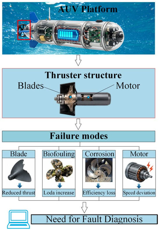
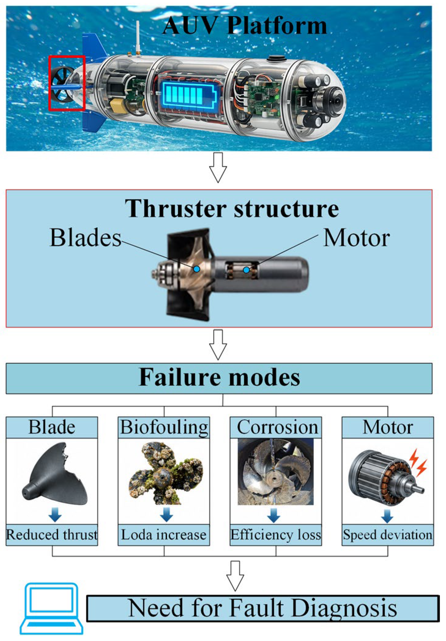
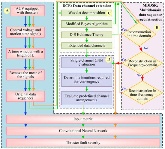
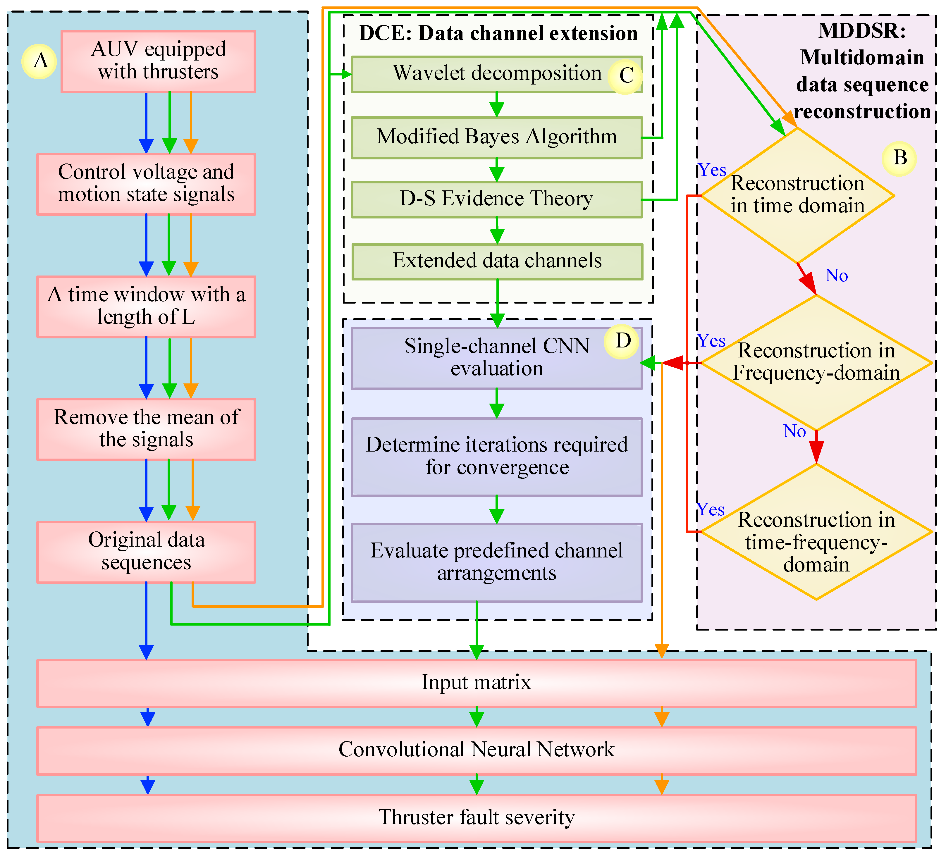
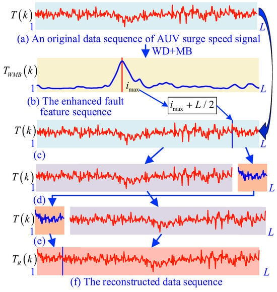
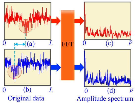
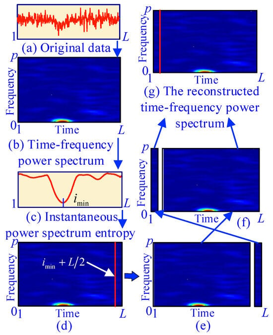
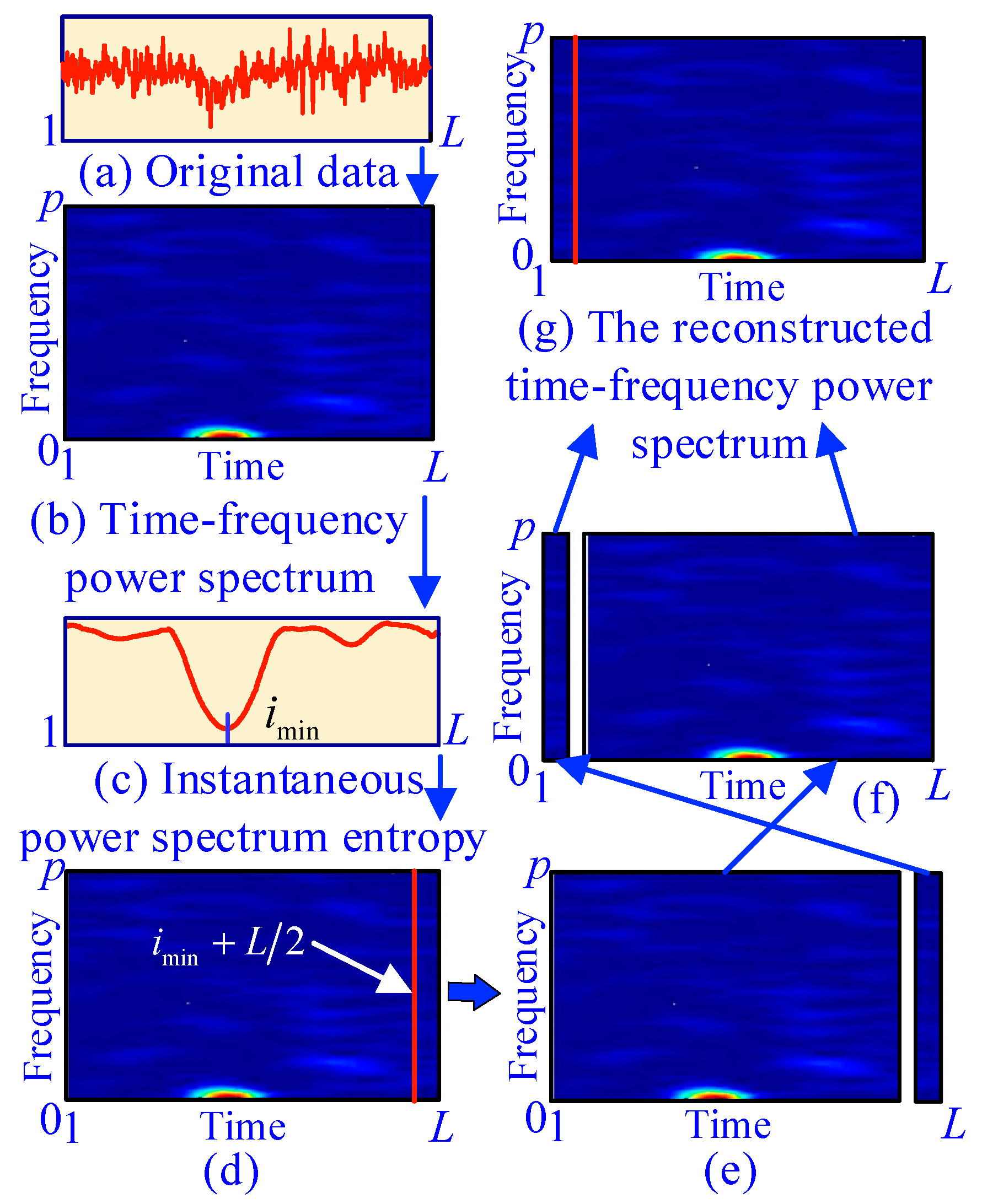
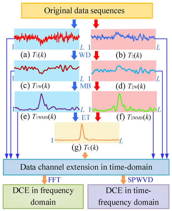
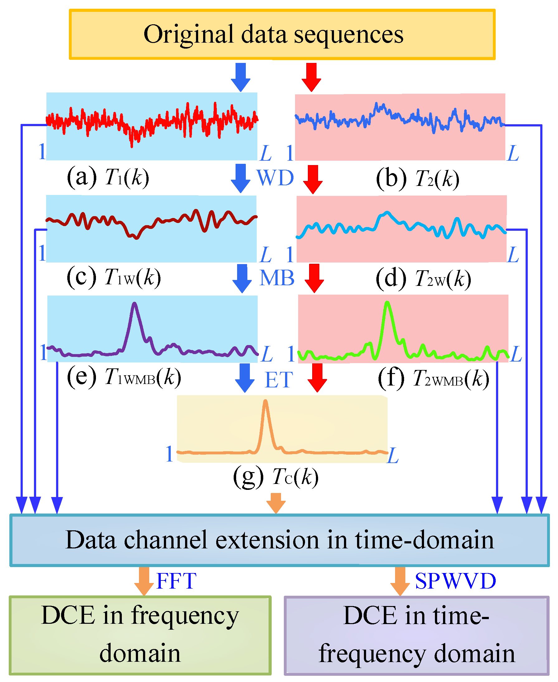
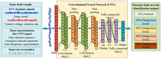
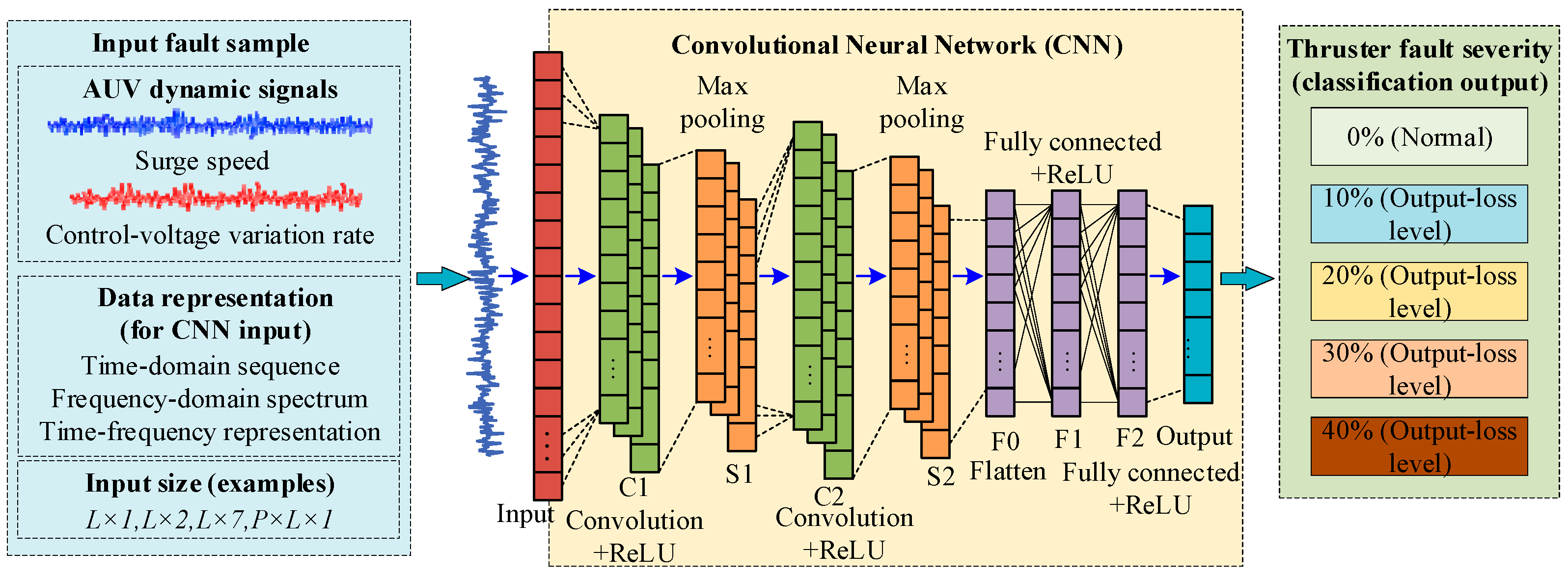
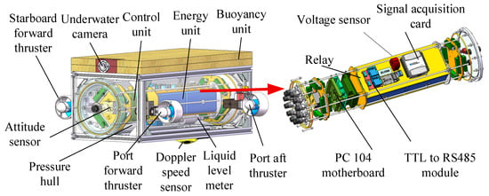
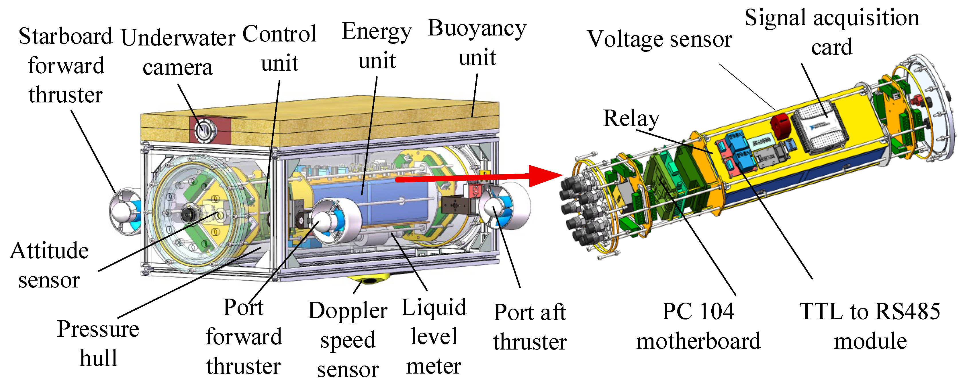
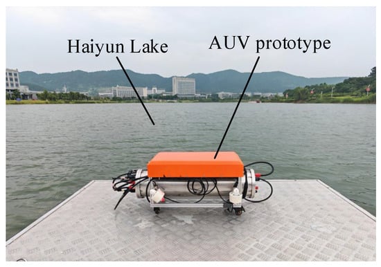
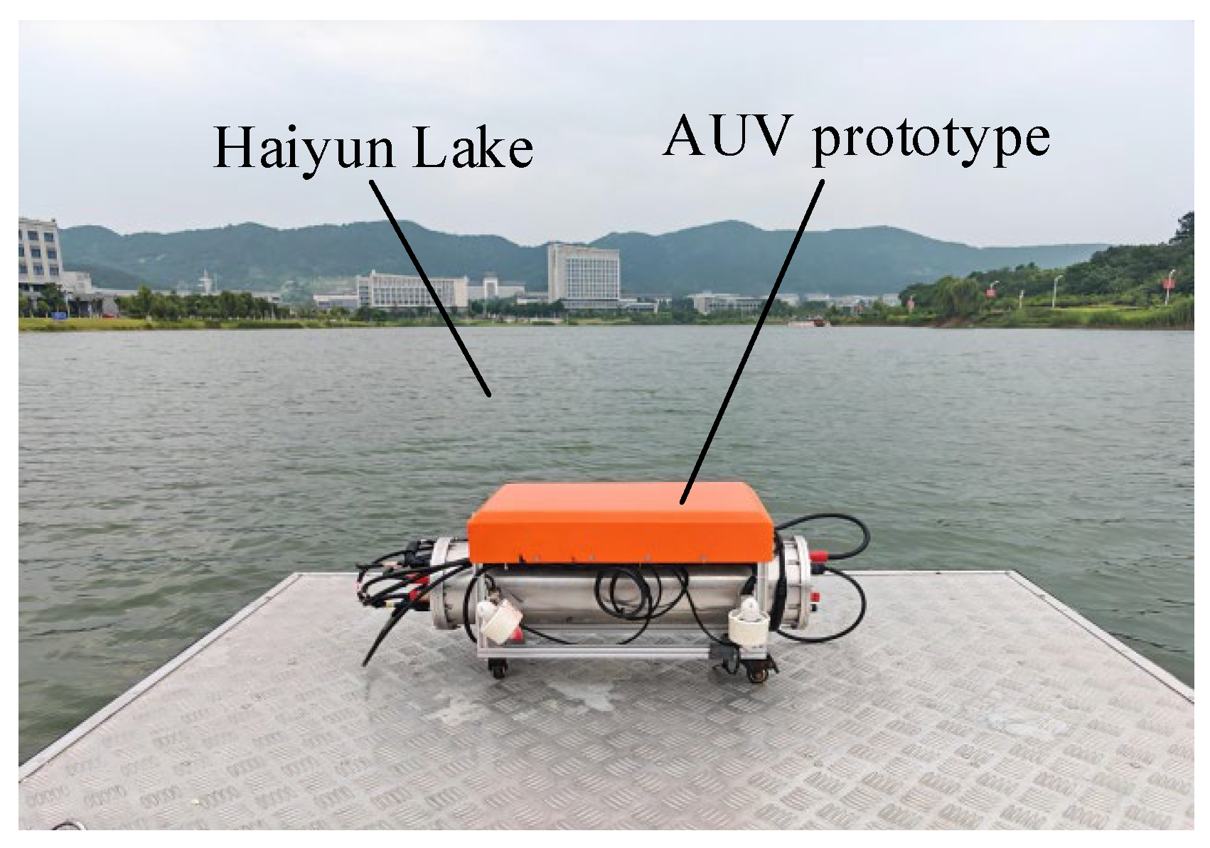
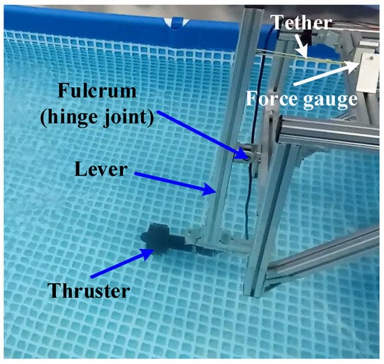
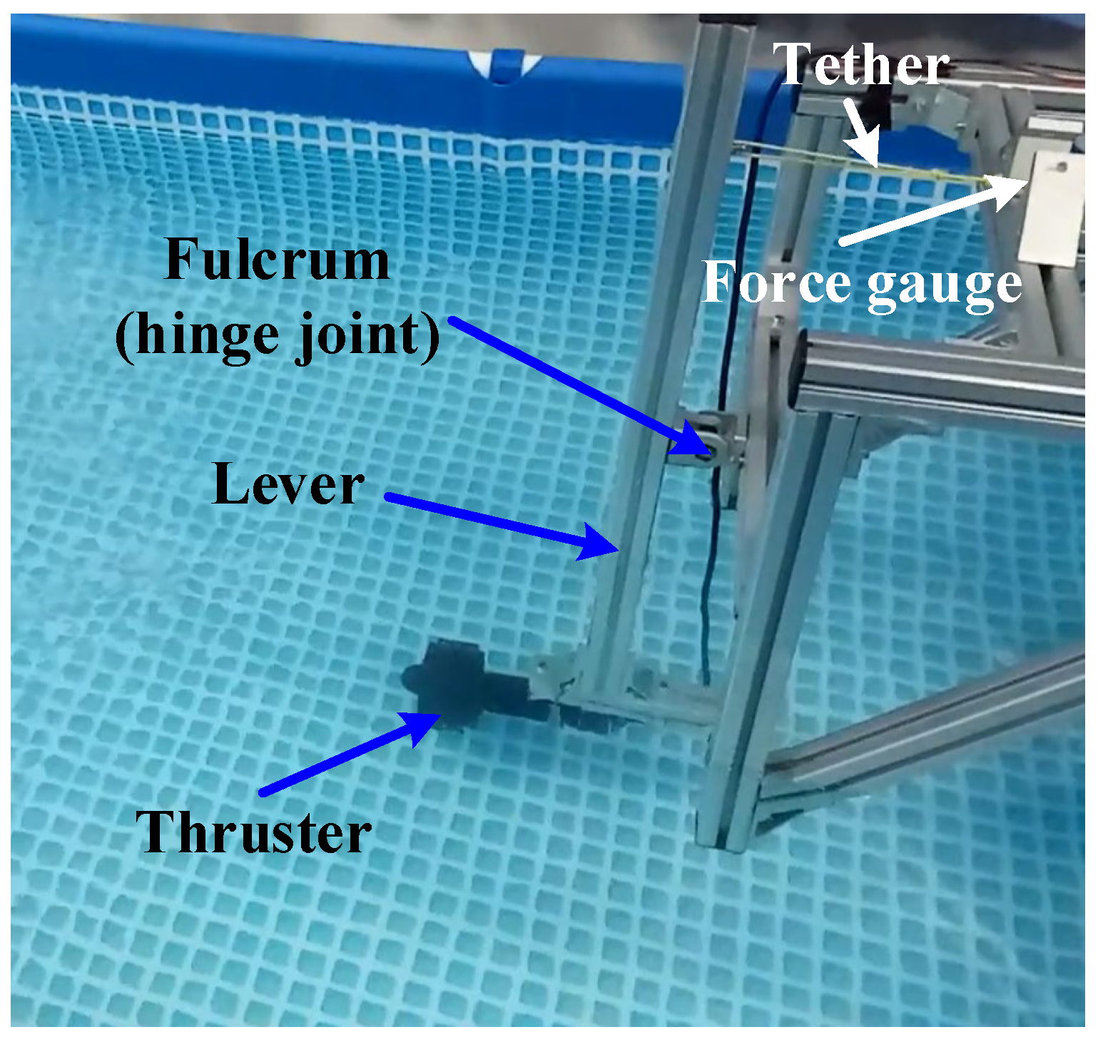
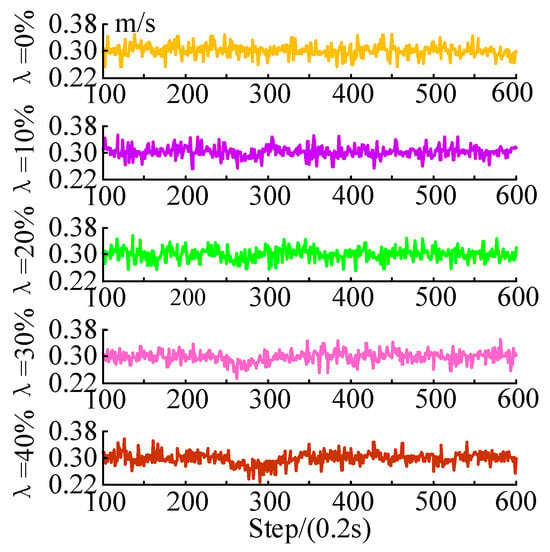
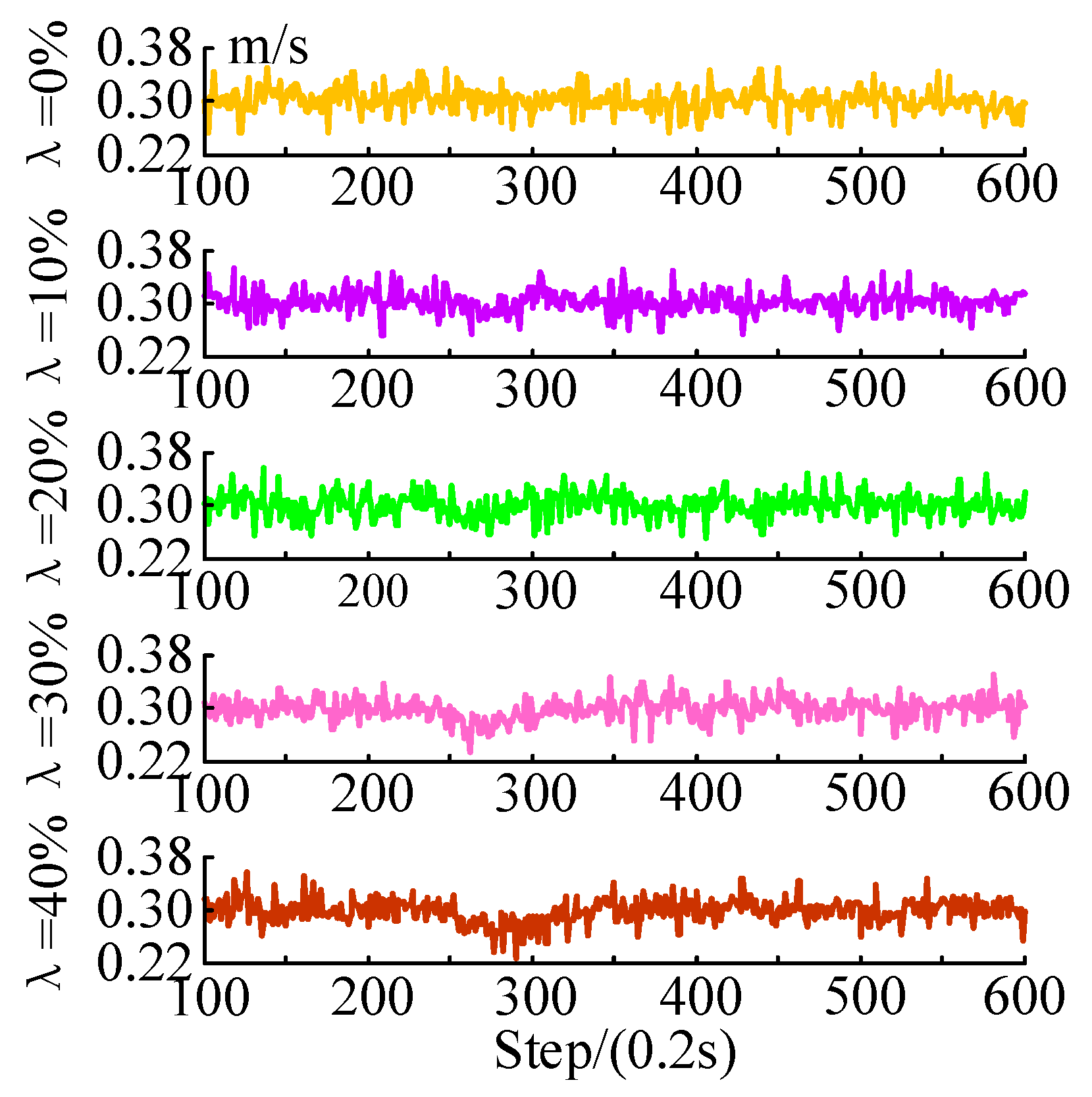
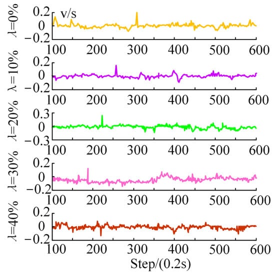
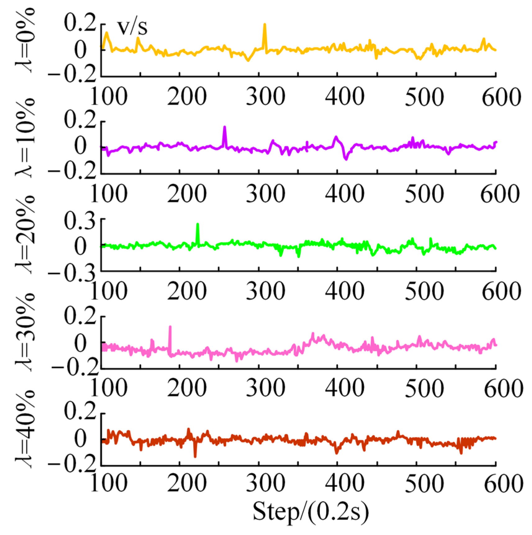
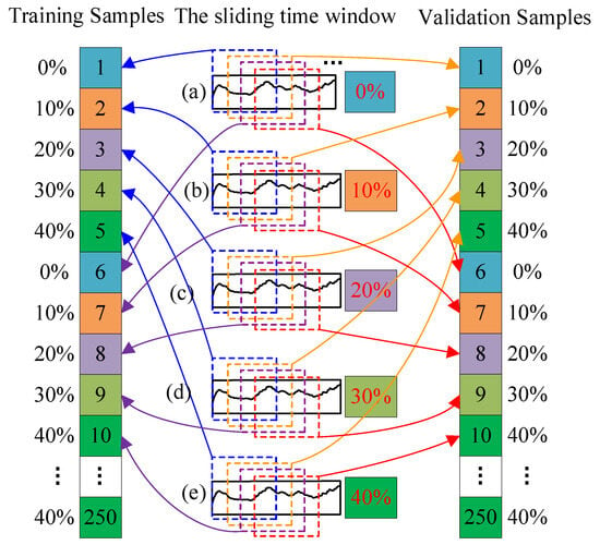
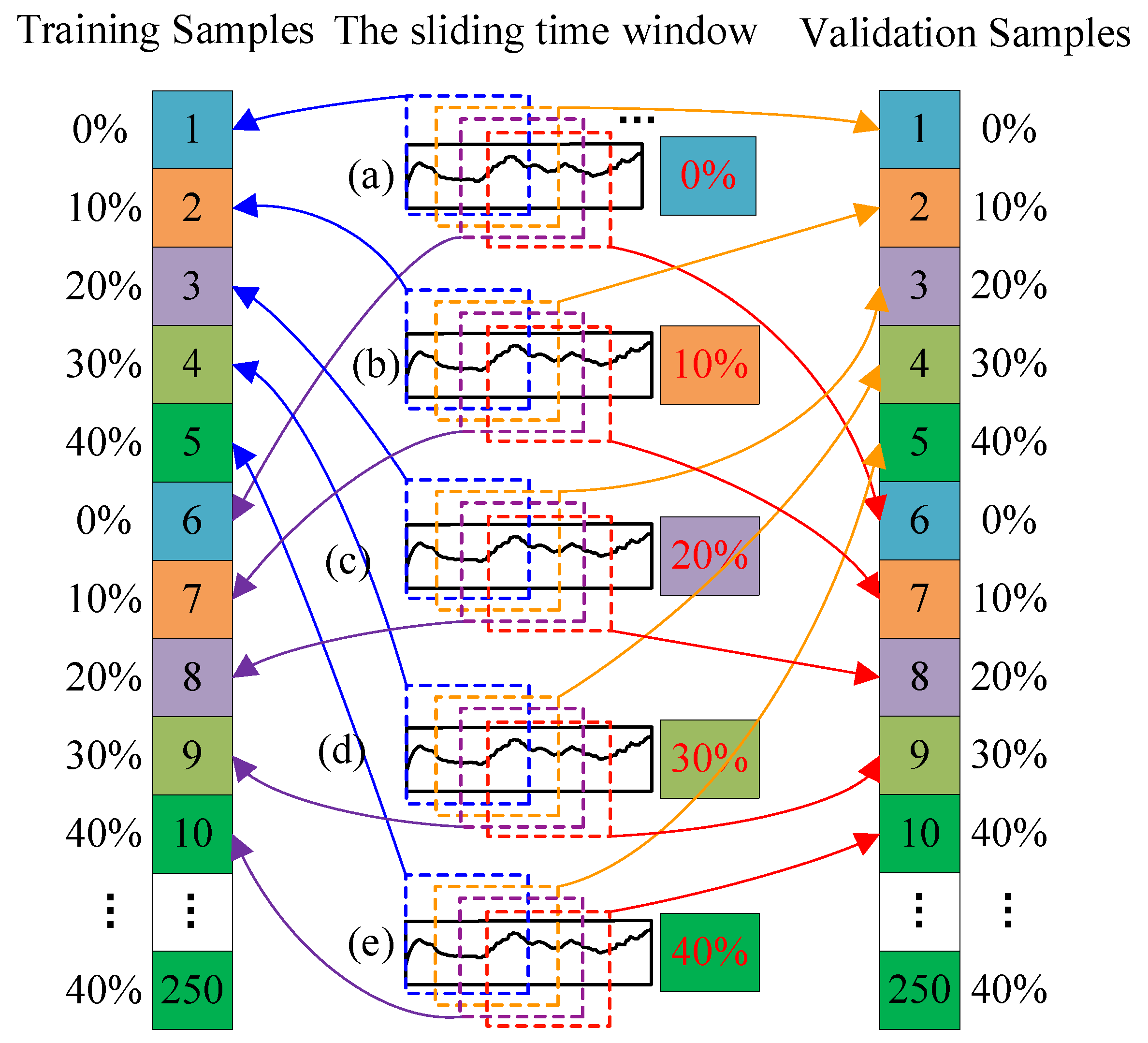
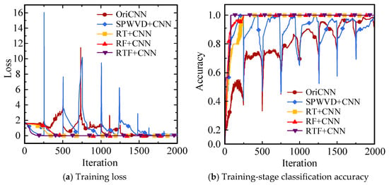
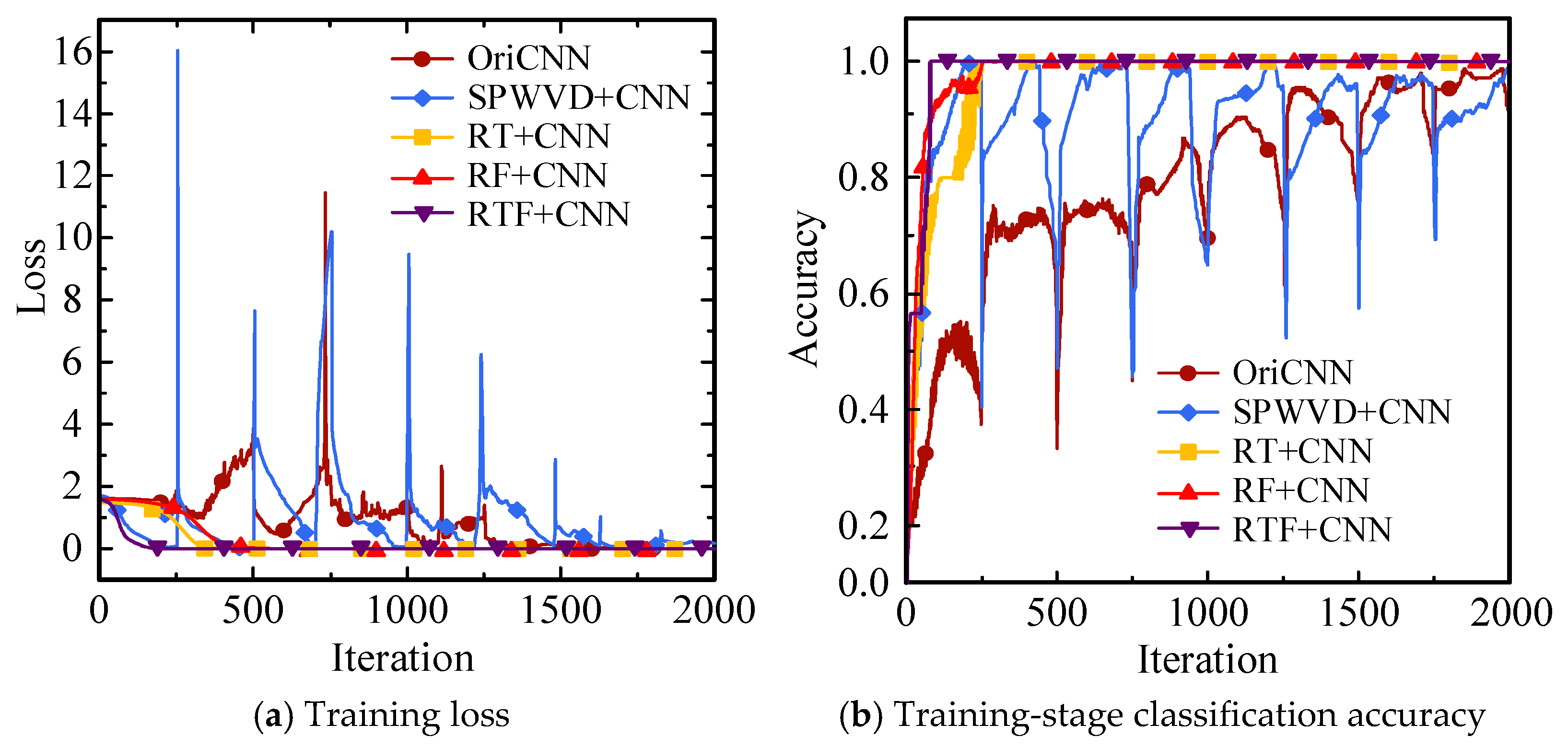
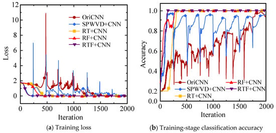
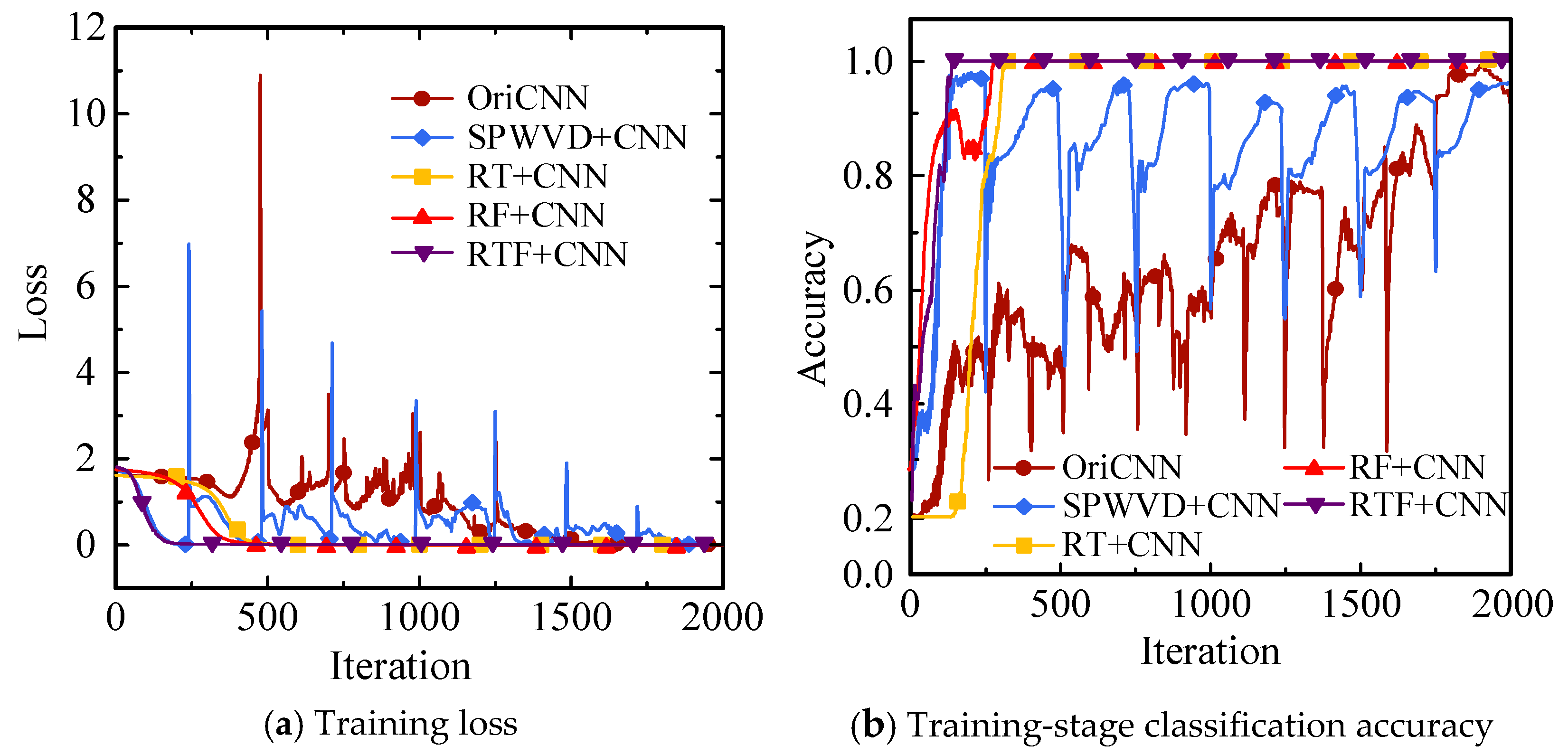
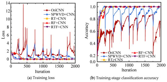
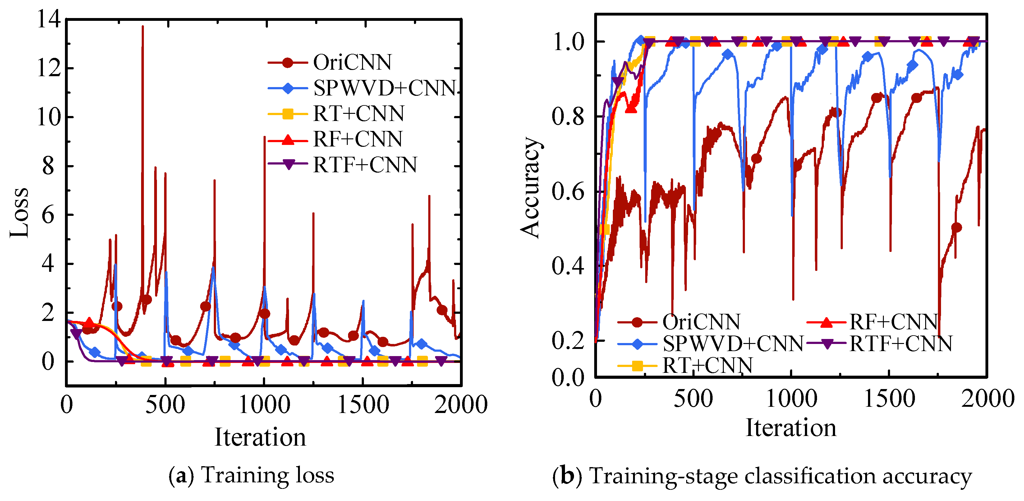
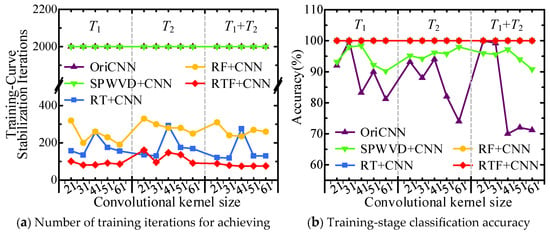
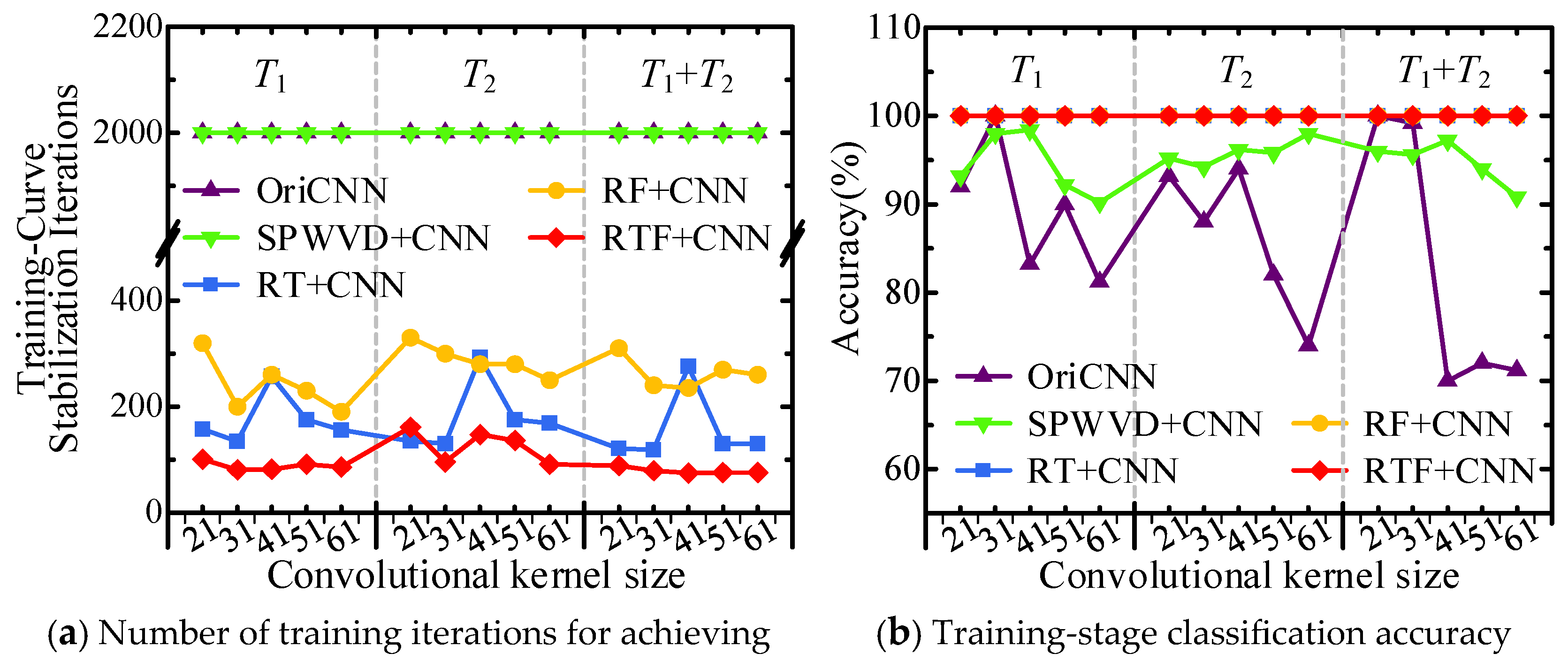
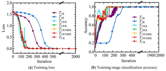
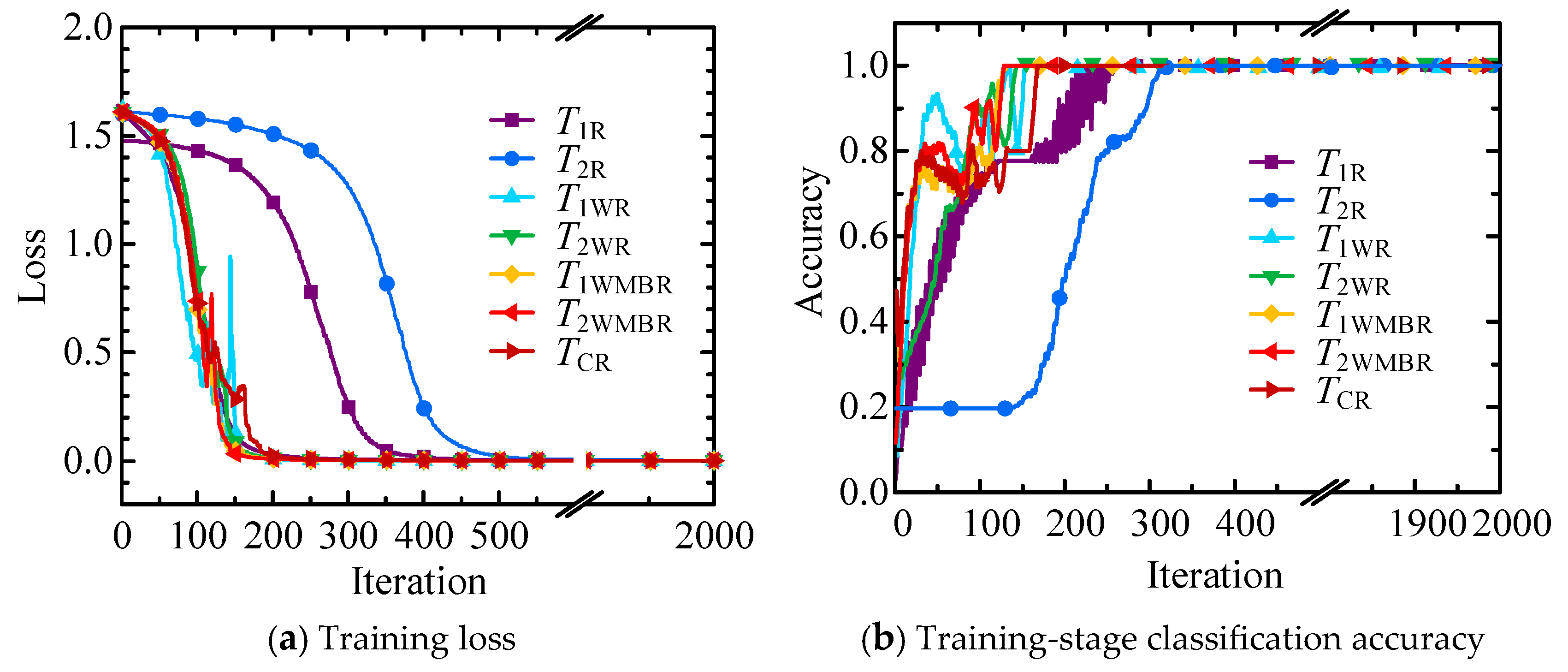
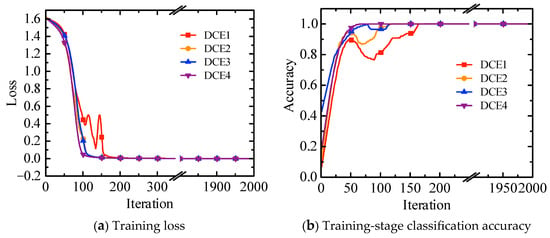
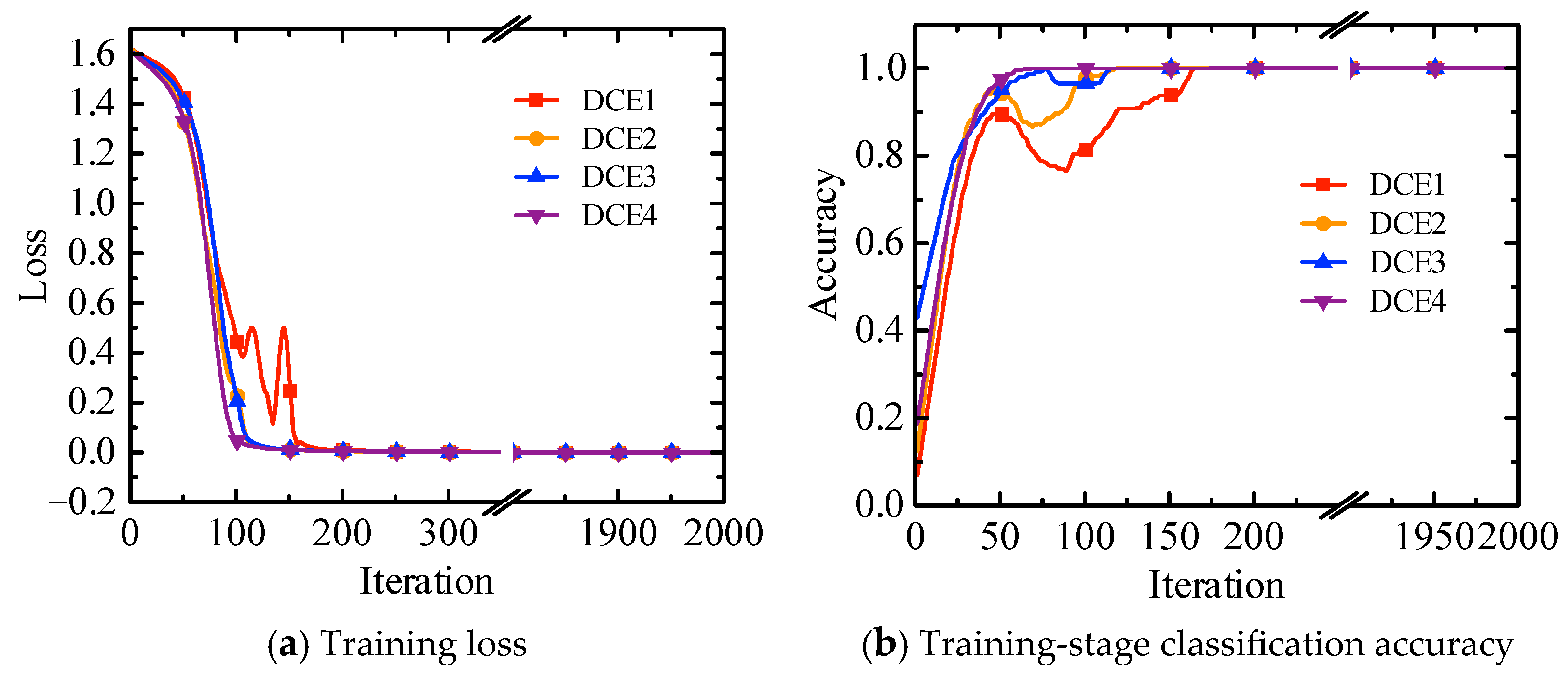
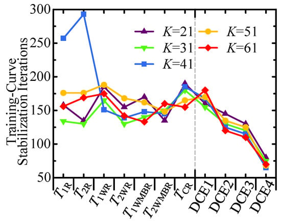
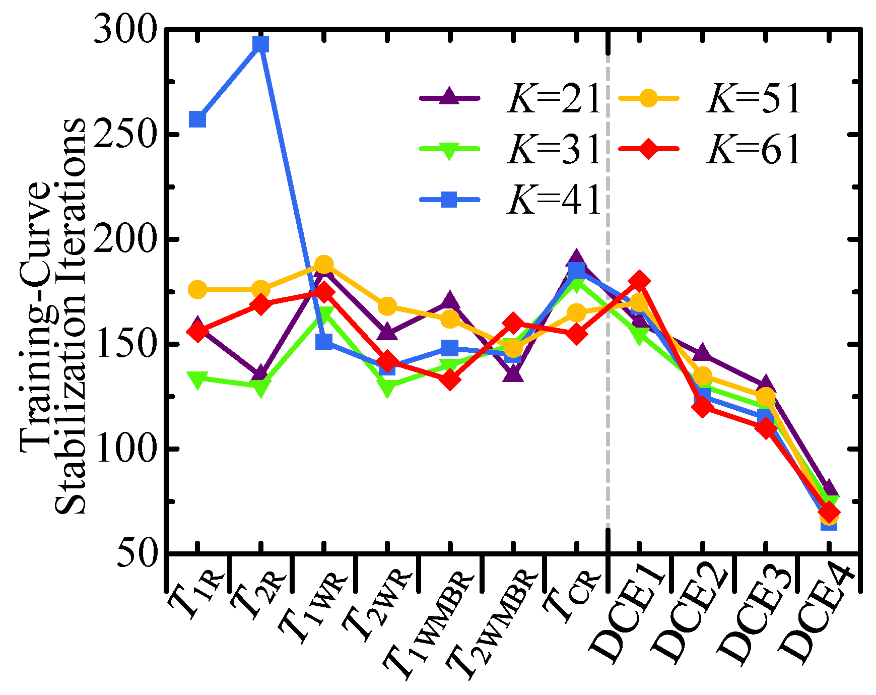
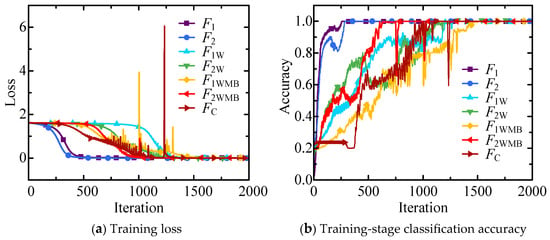
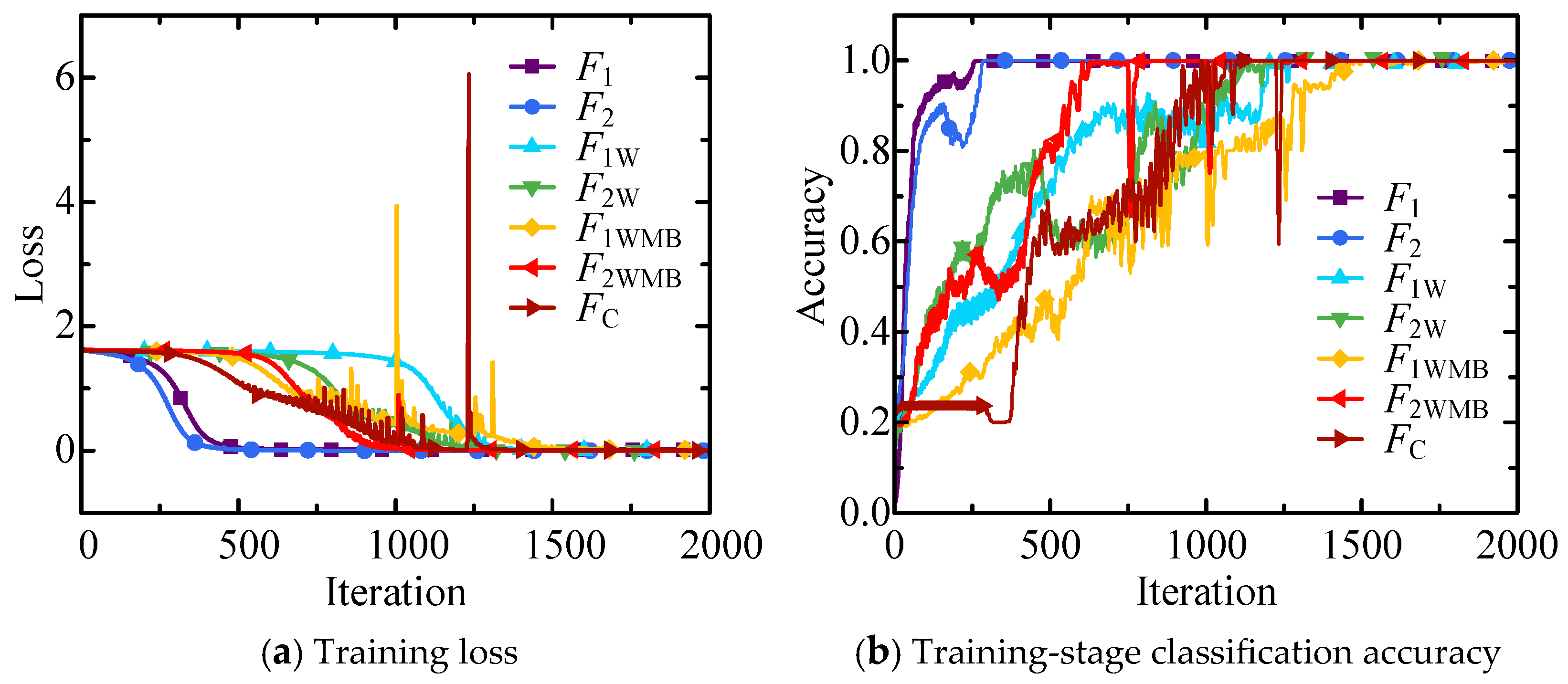
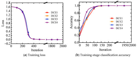
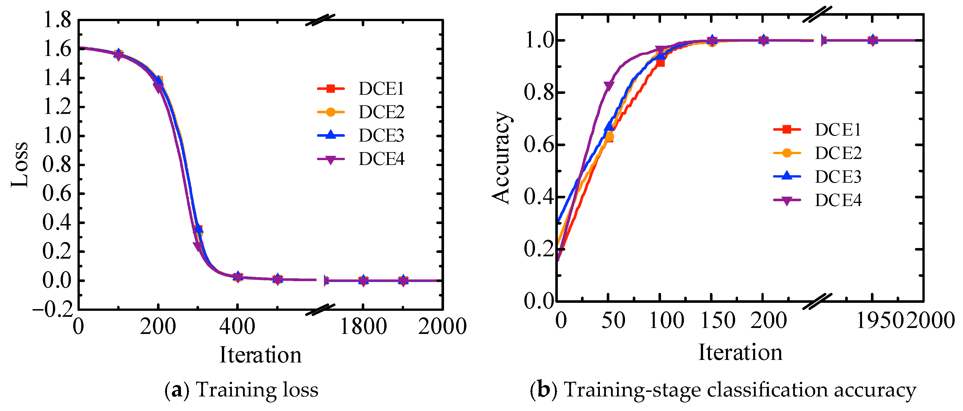
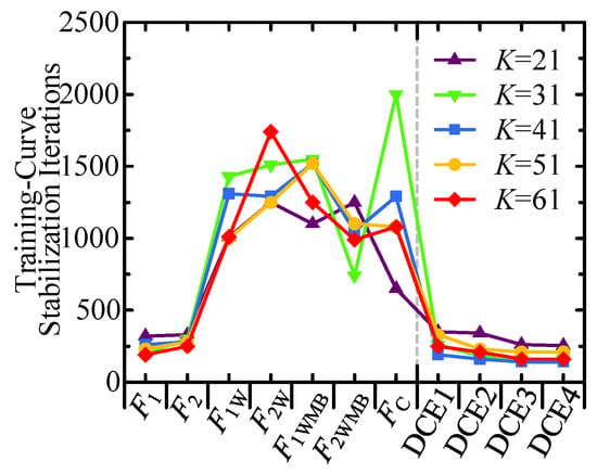
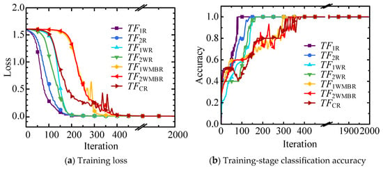
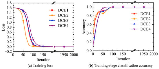
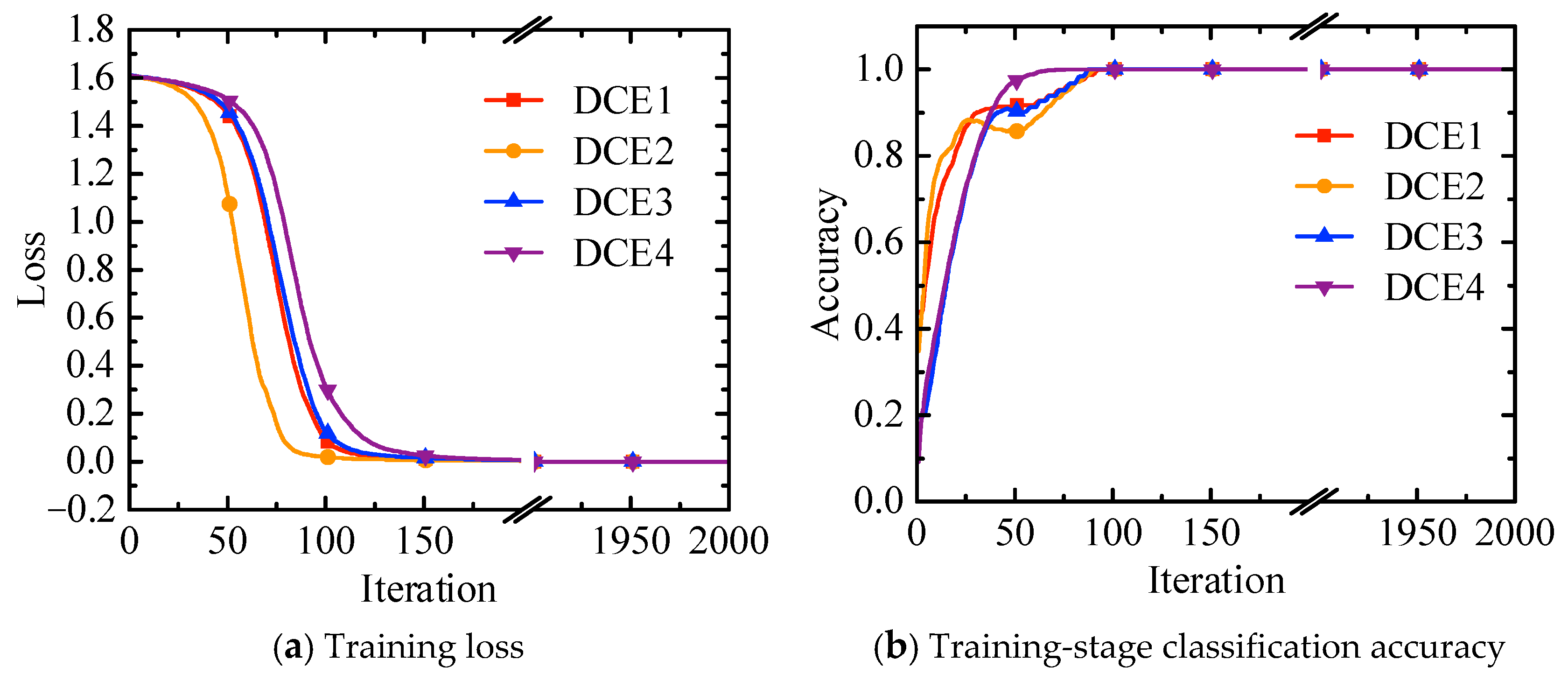
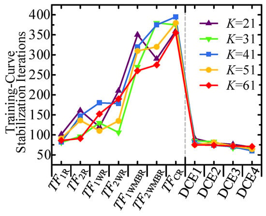
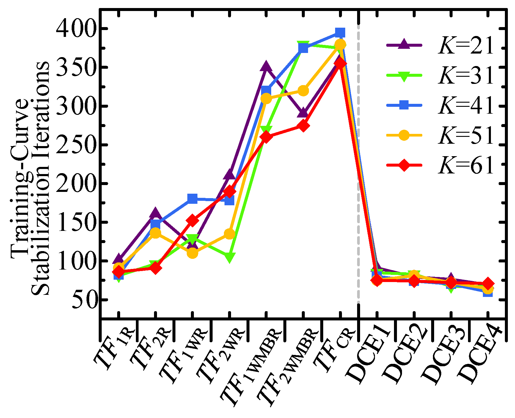

Disclaimer/Publisher’s Note: The statements, opinions and data contained in all publications are solely those of the individual author(s) and contributor(s) and not of MDPI and/or the editor(s). MDPI and/or the editor(s) disclaim responsibility for any injury to people or property resulting from any ideas, methods, instructions or products referred to in the content. |
© 2026 by the authors. Licensee MDPI, Basel, Switzerland. This article is an open access article distributed under the terms and conditions of the Creative Commons Attribution (CC BY) license.