


Abstract
The combined exploitation of marine wind and wave energy contributes to addressing pressing energy challenges. Satellite altimetry enables global synergistic assessment of these resources. Here, we utilize the longest altimeter observations available (Jason series, 1993–2024) to assess the spatiotemporal distribution, correlation, variability, and synergy of global wind and wave energy. Altimeter-derived wind speed and significant wave height were validated against buoy data, showing high consistency. Results indicate that wind and wave energy share similar spatiotemporal distributions. The Southern Ocean exhibits the most powerful and persistent resources, with moderate variability and correlation. Other energetic regions, including the Arabian Sea, North Atlantic, and North Pacific, show higher correlation and variability. Maximum covariance analysis (MCA) identified a leading mode of wind–wave co-variability, with a positive correlation between the expansion coefficients (r = 0.72). The result indicates a positive temporal association within the leading mode. The spatial patterns of the leading mode qualitatively resemble features associated with large-scale climate variability, including ENSO-related patterns. However, these similarities do not establish a direct statistical relationship with ENSO or demonstrate a causal climate influence. This study establishes satellite altimetry as a foundational tool for synergistic assessment of global wind and wave energy potential, providing a scientific basis for combined exploitation of marine energy resources.
1. Introduction
Global dependence on finite, non-renewable resources has led to severe environmental degradation and escalating energy crises. The combustion of fossil fuels constitutes a primary source of greenhouse gas emissions and a driving factor in global warming. Consequently, the development and utilization of renewable clean energy have become vital strategies for mitigating the adverse impacts of climate change and ensuring sustainable development [1,2]. Integrating renewable clean energy sources into the global energy matrix provides a practical approach to reduce greenhouse gas emissions and enhance energy security. Research, development, and deployment of renewable clean energy solutions are crucial for addressing energy insecurity and environmental challenges.
Marine wind and wave energy are key components of the renewable clean energy system, offering substantial potential for sustainable energy development. These energy resources possess distinct advantages, including abundance, source predictability, developability, and low environmental impact. Therefore, harnessing wind and wave energy can help optimize the global energy structure, contribute to sustainable development, and mitigate climate change. However, both wind and wave energy resources exhibit highly variable spatiotemporal distributions. Exploitation of either single energy source often suffers from issues such as intermittent energy supply and low efficiency. Combining wind and wave energy and taking advantage of their spatiotemporal complementarity can help alleviate these issues [3,4,5]. Assessing their joint spatiotemporal distribution is a fundamental step toward utilization. Understanding the patterns of availability in location and time is essential for identifying optimal sites and scheduling for energy exploitation. Performing a synergistic assessment of the distribution, correlation, and variability not only can improve project feasibility but also support long-term energy stability and sustainability.
Currently, single-source assessments of offshore wind or wave energy have been conducted in regional or global oceans. Wind energy assessments typically rely on sea surface wind speed, while wave energy evaluations depend on significant wave height (SWH), wave period, and other ocean parameters. Early studies used buoys and ship-based instruments to collect accurate in-situ measurements [6,7,8]. These platforms provided valuable data on ocean winds and waves, but such data are limited in spatial and temporal coverage, restricting most analyses to specific locations [9].
With the development of satellite technology, remote sensing and numerical modeling have become essential tools for assessing marine energy resources. Benefiting from high spatial coverage of satellites, satellite data, reanalysis datasets, and numerical models on the basis of wave physics and fluid dynamics knowledge have been successfully applied to wind and wave energy assessment at various scales, from regional coverage [10,11,12,13] to global [14,15,16]. For instance, numerical models such as WAVEWATCH-III (WW III) and reanalysis datasets like ERA-Interim have been employed to simulate wave conditions in regions including Hawaiian waters, the Arabian Sea, and the Bengal Bay, thereby enabling the identification of optimal locations for wave energy converters [17,18]. Research based on ERA5 and WW III datasets has revealed significant spatiotemporal variations in global offshore wind and wave energy distribution [16,19]. These methods have substantially advanced understanding of the spatiotemporal characteristics and variability of marine energy resources. Nevertheless, numerical models still face challenges due to limitations in wave dynamics understanding and lack of ground truth observations, resulting in considerable uncertainties [20,21,22]. Additionally, since wind and wave data were often derived from different sources, most previous studies have often focused on independent assessments of offshore wind or wave energy, with limited research on their synergy effects.
Using concurrent measurements of wind parameters such as wind speed, as well as wave parameters including wave height and wave period from the same platform is crucial for evaluating wind-wave synergy. Satellite altimetry can concurrently and directly measure ocean wind and wave data. This method uses radiometers and altimeters to measure sea surface wind speed and SWH, while deriving wave period from key parameters such as the backscatter coefficient. Of course, there are also various other remote sensing technologies that can be used for concurrent wind and wave observations. For instance, high-frequency (HF) radar can continuously monitor surface currents, wind, and waves in nearshore areas (up to 200 km offshore) [23], X-band marine radar can obtain ocean wind and wave information from radar images [24], and GNSS reflectometry (GNSS-R) techniques, including WaveTransNet, Hybrid CTN, and PA-CNN, can provide wind and wave measurement data with high spatio-temporal resolution at a relatively low cost [25]. However, these techniques are primarily suited to regional or coastal applications. Satellite altimetry offers advantages such as global coverage, high accessibility, repeatable measurements, and long-term observations, making it an ideal tool for assessment of global marine wind-wave energy resources [26,27,28]. Moreover, many studies have demonstrated that satellite altimeter data align well with buoy measurements, underscoring their reliability [29,30,31,32,33]. Although previous studies have demonstrated the feasibility of combined assessments using satellite altimetry in regional seas such as European coastal waters [28], no study to date has performed a synergistic assessment of global marine wind and wave energy using this technology.
This study aims to conduct a synergistic assessment of the spatiotemporal distribution, correlation, variability, and complementary variations of global marine wind and wave energy over the last 32 years (1993–2024) using satellite altimeter data. The primary objectives include: constructing a long-term, most consistently homogeneous satellite altimeter time series with inter-mission consistency assessment (T/P, Jason-1/2/3, and Sentinel-6A) available to date for a global synergistic assessment, providing an observation-based, model-independent benchmark; quantifying the correlation and frequency of high-energy events and variability indices to characterize the stability and temporal characteristics of the two resources, which is essential for hybrid energy planning; assessing the global wind-wave synergy using maximum covariance analysis (MCA) and establishing a preliminary qualitative link between the leading modes and large-scale climate patterns (ENSO, NAO, AAO). This climate-modulated synergy has not been previously demonstrated on a global scale using altimetry alone. Such studies will complement existing model-based assessments and provide a long-term observational benchmark for future research.
2. Data Sources
2.1. Satellite Altimeter Data
The successful implementation of the TOPEX/Poseidon (T/P) satellite mission in October 1992 marked the start of precise satellite altimetry and established a foundation for long-term monitoring of ocean dynamics from space. Subsequent successful missions, including Jason-1, Jason-2, Jason-3, and Jason-CS (Sentinel-6A), have provided seamless, high-accuracy datasets spanning over three decades [1,34]. These datasets enable global measurements of ocean topography, sea surface height, and other ocean environmental parameters at a 10-day resolution. Over the years, the Jason satellite series has played a pivotal role in monitoring and studying global sea level changes, ocean currents, wave heights, wind speeds, as well as other dynamic oceanographic parameters and their variations [35,36,37].
This study investigates the spatiotemporal characteristics and synergistic variations of global wind and wave energy over the last 32 years using altimeter data from T/P, Jason-1/2/3, and Jason-CS. The Geophysical Data Records (GDRs) provided by AVISO (https://www.aviso.altimetry.fr/) and EUMETSAT (https://www.eumetsat.int/) are employed, which includes T/P data from January 1993 to August 2002, Jason-1 data between January 2002 and January 2009, Jason-2 data between July 2008 and September 2016, Jason-3 data (February 2016 to April 2022), and Sentinel-6A data (September 2021 to December 2024) (Figure 1 and Supplementary Table S1). The variables used include time, longitude, latitude, wind speed, and SWH. Although the T/P, Jason-1/2/3, and Sentinel-6A missions have slightly different antenna designs and footprint diameters (typically 2–3 km for Ku-band altimeters), these differences are minimal for global-scale wind and wave assessment. To ensure spatial consistency, we applied the following procedures: (1) All along-track 1 Hz data (approximately 7 km spacing) were used without further footprint-specific filtering, as the spatial scales of wind speed and SWH variability relevant to energy assessment are much larger (>50 km). (2) The data from all missions were interpolated onto a common 1° × 1° global grid using continuous curvature splines, which effectively homogenizes any remaining footprint-induced sampling differences. (3) Overlapping observation periods of seversal months between successive satellite missions were employed to assess inter-satellite consistency by comparing global mean values during these overlapping intervals. By averaging the observations from the two satellites during the overlapping period, we construct a 32-year time series spanning January 1993 to December 2024.
Figure 1.
Timeline of the Jason data used in this study; the periods between the two red dotted lines indicate the synchronized observation of the two satellites.
2.2. Buoy In-Situ Measurements
To calibrate altimeter data effectively, it is necessary to establish a long-term, high-quality database of in-situ wind speed and wave height measurements from buoys. Buoy-based measurements are an effective way to monitor the marine environment in situ, providing physical parameters related to water temperature, wind, and waves, and so on. Buoy data are widely acknowledged for their high quality and reliability, making them valuable for validating altimeter data [29,30,31]. This study employs historical buoy observations from the National Data Buoy Center (NDBC, https://www.ndbc.noaa.gov/), which include buoy geographical locations, wind direction, wind speed, SWH, average wave period, and sea level pressure with one record per hour. We selected buoy stations meeting specific criteria: availability, sufficient temporal overlap with the satellite records spanning 1993–2024, and locations within 50 km of altimeter ground tracks. Ultimately, a total of 68 buoy stations were selected globally. The number of stations contributing to the final validation differed between wind speed and significant wave height because the availability of valid satellite–buoy collocations varied by variable and station. Accordingly, the validation statistics for wind speed and significant wave height were calculated separately using the available valid collocations for each variable. Stations without valid collocations for a given variable were not included in the corresponding validation statistics. The initial set of 68 stations therefore represents the candidate station pool rather than the number of stations necessarily contributing to every validation analysis. Station-specific observation periods, collocation counts, and satellite mission coverage are documented in Supplementary Table S2. The variables time, longitude, latitude, wind speed, and SWH from buoy data are extracted and compared with corresponding altimeter data to ensure accurate validation.
Unlike satellite altimeters, which estimate wind speeds at 10 m above the sea surface (U10), buoys of different types measure wind speed at varying heights corresponding to their anemometer positions (anemometer height). To align with altimeter-derived U10, the wind speeds measured by buoys must be converted to neutral winds at 10 m using the following log-profile relation, which assumes a neutrally stable air-sea boundary layer [30,33].
where denotes the wind speed measured at a height z above sea level, is the von Kármán constant (approximately 0.4), represents the roughness length, and denotes the drag coefficient. The drag coefficient will vary with both sea state and wind speed [38]. Given that does not have a significant influence on the final satellite wind speed. and is used in this study with reference to [33].
3. Validation of Altimeter Data
3.1. Inter-Mission Consistency Assessment
To construct long-term time series of global wind and wave energy, it is essential to assess altimeter wind and wave measurements and verify the homogeneity and consistency of various satellites. Indeed, satellites are always validated a few months after launch, during a dedicated commissioning phase [29,39]. Inter-mission consistency is preliminarily assessed by comparing global mean values during overlapping mission periods, which can provide an initial assessment of large-scale consistency between missions. We compare global mean wind speeds and SWHs from synchronized observation cycles of inter-missions. For each 10-day cycle, global mean values were obtained by latitude-weighted averaging over all valid 1 Hz along-track measurements, with weights proportional to the cosine of latitude [19]. The inter-mission discrepancies are estimated and shown in Figure 2. Detailed overlap statistics are provided in Supplementary Table S1. The standard deviation (STD) of wind speed difference between multi-missions varies from 0.07 m/s to 0.11 m/s. The STDs of SWH differences between multi-missions are all 0.01 m. The validation results suggest that the accuracies of satellites T/P and Jason-1/2/3/CS are highly consistent at the global-mean level. So, no additional numerical bias correction was applied to the individual satellite records on the basis of these overlap comparisons before merging. It is feasible to use this series of satellites to construct long-term time series of altimeter wind and wave measurements. However, this study does not provide a direct assessment of pointwise inter-mission bias or time-dependent instrumental drift.
Figure 2.
Comparison of wind speed (left) and SWH (right) from T/P and Jason satellites in synchronous observation period. (a–d) Wind speed comparison between T/P and Jason-1, Jason-1 and Jason-2, Jason-2 and Jason-3, and Jason-3 and Sentinel-6A, respectively. (e–h) SWH comparison between T/P and Jason-1, Jason-1 and Jason-2, Jason-2 and Jason-3, and Jason-3 and Sentinel-6A. In each panel, the mean difference and standard deviation (STD) are annotated, and the corresponding satellite cycles are indicated on the secondary x-axis.
3.2. Validation Against Buoy In Situ Measurements
To evaluate the performance of the satellite altimeter, the altimeter data was validated against available buoy measurements via the collocation method [6,40]. Comparing altimeter data with in situ measurements presents inherent complexity, as they are measuring spatiotemporally varying fields. Consequently, discrepancies may arise even though both tools yield accurate estimates [6]. Comparison between altimeter and buoy data requires specific spatial and temporal separation criteria. Acceptable standards for effective comparison include a spatial domain varying from 0 to 150 km and a temporal domain spanning 0 to 1.5 h [31]. Notably, spatial separation criteria of 50 km and temporal criteria of 30 min are widely applied in calibration studies using the collocation method [27,29,40].
In this study, a total of 68 buoy stations were initially selected to validate altimeter-derived wind speeds and SWHs for the period 1993–2024, the locations and information are shown in Figure 3a and Table S2. The criteria of 50 km and ±30 min are used to obtain collocation points (Figure 3b). Since not all buoys can simultaneously measure wind and wave data, there is no exact correspondence between buoys used for calibrating wind speed and SWH. The validation datasets comprised variable-specific subsets of the 68 candidate NDBC buoy stations. Based on the available valid collocations, wind-speed validation included 56 stations and 86,952 paired observations, whereas SWH validation included 36 stations and 33,357 paired observations. Comparisons between altimeter-derived and buoy-measured wind speed are shown as a time series plot and a scatter plot in Figure 3c,d. Some standard error metrics, including the correlation coefficient (Pearson coefficient r), mean absolute error (MAE), bias, and root-mean-square error (RMSE), are used to evaluate the data (Supplementary Table S3). The time series distributions of altimeter and buoy wind speeds are highly consistent, showing some seasonal characteristics. The correlation coefficient between the altimeter and buoy wind speed is 0.8708 (R2 = 0.758), with a bias of 0.50 m/s, an RMSE of 1.75 m/s, and a MAE of 1.33 m/s. Similarly, Figure 3e,f show the comparison between altimeter and buoy SWH. The correlation coefficient for SWH is 0.9557 (R2 = 0.913), with a bias of −0.02 m, an RMSE of 0.32 m, and a MAE of 0.20 m. To assess station-level validation performance, validation statistics were calculated separately for each buoy station and variable using the corresponding valid satellite–buoy collocations. The station-wise wind-speed and SWH validation statistics are provided in Supplementary Tables S4 and S5, respectively. These results are consistent with the findings of [30], who calibrated long-term altimetry satellite wind speeds and wave heights using buoy data. These results indicate that the wind speeds and SWHs retrieved from satellite altimeters are in high agreement with buoy in situ measurements, and the accuracy of altimeter measurements is comparable to that of buoy measurements. As such, it is shown that the dataset we used is an extensively validated and homogeneous multi-satellite record.
Figure 3.
Comparison of altimeter-derived wind speed and SWH against NDBC buoy measurements. (a) Geographic locations of the 68 NDBC buoy stations, marked with red stars. (b) Schematic of the collocation criteria (50 km and ±30 min); the red dashed circle indicates a 50-km radius around center buoy. (c) Time series and (d) scatter density plot of altimeter-derived versus buoy-measured wind speed, with the 1:1 line (red dashed) and regression line (black solid). (e) Time series and (f) scatter density plot of altimeter-derived versus buoy-measured SWH.
4. Methods for Energy Estimation
4.1. Calculation of Wind Power Density
Basically, wind energy calculation relies on the knowledge of fundamental geometry and the physical principles behind kinetic energy. The kinetic energy of wind is defined as the energy transferred by air moving vertically through a cross-sectional area at a given wind speed. It is mathematically expressed as follows [41]:
where is the kinetic energy, is the air mass, and represents the wind speed.
The air mass can be expressed as the product of air density and the volume of air traversing a cross-section over a given time period. Therefore, the kinetic energy can be rewritten as:
where is the sea surface air density, A is the cross-sectional area, and t is the time period.
Through mathematical derivation, wind power density, defined as the wind potential in per unit area per unit time, serving as the fundamental unit for estimating energy stored within the wind, is expressed as follows:
where represents the wind power density in W/m2. In this study, the air density is taken as 1.292 kg/m3. This value provides a consistent basis for global comparison. Since wind power density is linearly proportional to air density, the assumption mainly affects the absolute magnitude of wind resource estimates rather than their large-scale spatial patterns.
Based on the above equations, global wind power density was calculated during the period 1993–2024 using altimeter-derived wind speeds. The wind speed has a temporal resolution of 10 days.
4.2. Calculation of Wave Power
Wave power, or wave energy flux, defined as the wave energy per unit crest length, is a key parameter for understanding wave generation, propagation, and dissipation. This parameter is typically derived from a variance spectral density function which characterizes the distribution of wave amplitudes, frequencies, and directions [42,43].
Wave power is calculated using the following expression [11]:
where P denotes wave power per unit wave crest length (kW/m), represents the SWH with unit of meters, is the energy period in seconds, g is the gravitational acceleration (9.81 m/s2) and denotes the density of seawater (assumed to be 1025 kg/m3).
Satellite altimetry has a limitation that it does not directly measure wave period data required for wave energy calculation. Therefore, the energy period must be estimated from other variables. Several empirical algorithms exist for estimating wave period from satellite altimetry, including: the method of Hwang et al. [44] estimates peak period (Tp) using wind speed (U10) and significant wave height (Hs); the model of Gommenginger et al. [45] estimates zero up-crossing, mean, and peak periods using Ku-band backscatter (σ0) and Hs; the parametric model of Mackay et al. [46] and the genetic algorithm approach [47]. We adopt Hwang’s method for four reasons. First, it requires only U10 and Hs—both directly measured and validated against buoys (Section 3.2)—avoiding the sensitive backscatter coefficient. Second, it is physically based and computationally efficient for 32 years of global data. Third, comparative evaluations confirm its reliability: Chu et al. [48] found that Hwang’s method yields accuracy comparable to other empirical approaches. Fourth, Hwang’s method has been widely used in wave energy assessments for the Gulf of Mexico [43,44], South China Sea [27], and in Wave Energy Converters (WECs) power production [49]. It can be used to calculate the peak period Tp as follows:
where is wind speed and is gravitational acceleration.
The energy period is then approximated as:
where is a coefficient dependent on the wave spectrum shape (for example, the corresponding value for the Pierson-Moskowitz spectrum is 0.86) [27]. According to references [27] and [49], the different coefficient used will not affect the period value significantly. Moreover, because wave power scales with Hs2 (P ∝ Hs2·Te), Hs remains the dominant control, while uncertainties in Te have a secondary effect. So, we follow the recommendations for global wave energy assessment by setting in this study. Finally, the global wave power was calculated for every 10 days during 1993–2024 using altimeter-derived SWHs and the estimated energy period.
The Hwang-derived energy period () depends on both significant wave height () and wind speed (). Because is also used to calculate wind power density, the resulting wind–wave correlation and MCA may contain a mathematical coupling through the shared term. We quantify how much of the reported wind–wave co-variability is attributable to this coupling in Supplementary Section S1. Specifically, three controlled experiments were designed to isolate the contribution of the concurrent term in the period estimation, which results are shown in Supplementary Figures S1 and S2 and Table S6. The results from the three sets of experiments were highly consistent, indicating that wind-wave co-variability exhibits a certain degree of robustness with respect to the period estimation. We also compared the estimated energy period with the NDBC buoy average wave period for further validation. The results (see Figure S3) showed a bias of 0.529 s, an RMSE of 1.806 s, and a correlation coefficient of 0.792, indicating that the empirical relationship captures the overall variability of wave periods while containing uncertainties.
4.3. Calculation of Correlation and Variability Coefficient
To evaluate the correlation between marine wind and ocean wave energy resources, the Pearson product-moment correlation coefficient is applied to the wind power density and wave power time series. The mathematical expression is as follows:
where represents the correlation coefficient, N is the length of the time series, is the time lag between wind and wave energy (in this study ). and are the mean values of wind and wave energy, respectively, while and are the corresponding standard deviations. The correlation coefficient varies between −1 and 1, where −1 indicates perfect negative correlation, while 1 indicates perfect positive correlation. If the resources are uncorrelated, then .
To assess temporal variability, the coefficient of variation (COV) and monthly variability indicator (MVI) are used [28,50]. The COV measures interannual variability. A high value indicates large year-to-year fluctuations in energy resources, implying lower predictability and higher long-term investment risk. A low COV suggests stable and reliable conditions for multi-year energy planning. The MVI quantifies intra-annual (monthly) variability. A high MVI reflects strong seasonal fluctuations, which may require seasonal energy storage or hybrid system optimization. A low MVI indicates weak seasonal cycles, suggesting more consistent month-to-month resource availability. Employing these two indices enables the assessment of global wind and wave energy stability across different time scales. The COV is defined as the standard deviation normalized by the average of the energy time series:
The MVI is calculated as:
where and are the maximum and minimum values of the monthly energy time series, and is the annual average.
5. Results
5.1. Annual Spatial Distribution
Using T/P and Jason-series altimeter wind speeds and SWH data from 1993 to 2024 and the methodology described above, this study computed global along-track wind power density and wave power at a 10-day temporal resolution. To investigate the spatial distribution characteristics, the along-track energy values are interpolated onto a global grid using adjustable tension continuous curvature splines with tension 0.25. Additionally, grid cells affected by land contamination were removed using a land-sea mask. No explicit minimum observation-count threshold was imposed on individual grid cells in the original gridding procedure. To assess the sensitivity to the gridding procedure, we selected three months of data, gridded them at a 2° resolution, then compared them with the 1° grids, and performed track-segment holdout cross-validation. The spatial distributions of wind speed and SWH at both resolutions, along with their differences, are shown in Supplementary Figures S4–S6. We also statistics the sampling rate for the 1° grids, the results of which are shown in Supplementary Table S7. The statistical results of the differences between 1° and 2° grids and the cross-validation are presented in Supplementary Tables S8 and S9. The results showed that both resolutions reproduced highly similar large-scale spatial structures, indicating that the large-scale spatial patterns and conclusions of this study are robust to the gridding resolution. The same interpolation settings were applied consistently to all months and variables. Finally, monthly, seasonal, and annual averages are derived to characterize the mean spatial pattern.
Figure 4 presents the spatial distributions of global annual mean wind speed, SWH, wind power density, and wave power. Wind and wave energy closely follow the spatial patterns of wind speed and SWH, respectively, as expected given their direct dependence on these variables. Notably, both energy types exhibit significant regional differences across the global ocean. Wind speeds in most regions exceed 3 m/s, corresponding to wind energy densities greater than 200 W/m2. The Southern Ocean shows the highest wind speeds (8–13 m/s) and wind energy densities (600–1400 W/m2). Similarly, the North Pacific Ocean and the North Atlantic Ocean have relatively high wind speeds (8–11 m/s) and wind energy densities (600–1100 W/m2). This observed phenomenon may be influenced by the presence of low-pressure systems and the strong westerlies at high latitudes. Other regions with relatively high wind speeds (greater than 7 m/s) and wind energy densities (greater than 400 W/m2) include the Indian Ocean, Arabian Sea, Bay of Bengal, Tropical Pacific, and mid-to-low latitude Atlantic, potentially affected by monsoon dynamics.
Figure 4.
Spatial distribution of global annual mean wind speeds (a), wind power density (b), SWHs (c), and wave power (d).
In contrast, equatorial regions show significantly lower wind speeds and energy densities. Coastal areas such as Somalia, Southeast China, and the Caribbean are characterized by high wind speeds and wind energy densities, indicating strong exploitation potential. These distribution patterns are largely consistent with previous findings from [15], based on multi-platform microwave observations and QuikSCAT, ASCAT, and WindSAT data, respectively. This consistency underscores the reliability of altimetry data for wind energy assessment.
SWH and wave power distributions (in Figure 4c,d) show similar trends. Most ocean regions have SWHs greater than 1 m and wave power above 10 kW/m. The Southern Ocean westerlies exhibit the highest values, reaching 5 m and 140 kW/m, respectively. As with the wind energy distribution, the North Atlantic and North Pacific westerlies, along with parts of the Indian Ocean, Arabian Sea, Bay of Bengal, Tropical Pacific, and mid- to low-latitude Atlantic, also have relatively high SWHs (2–3.5 m) and wave power (40–90 kW/m). Around the coast of Somalia, the China Sea, and the Caribbean, SWHs and wave power are slightly higher, but not as significant as wind energy.
Identifying regions possessing co-located high wind and wave energy is essential for optimizing resource utilization and making informed decisions [51]. In this study, high-energy regions and high-energy-event frequency were characterized using two distinct percentile-based measures. First, high-energy regions were identified from the long-term mean wave-power field. The temporal mean was calculated at each grid cell over 1993–2024, and the 90th percentile was then calculated across all valid ocean grid cells in this spatial field. Grid cells with long-term mean wave power exceeding this spatial threshold were classified as high-energy regions. This measure identifies areas with comparatively high long-term mean resource levels.
Second, high-energy-event frequency was calculated using a global threshold derived from the complete monthly wave-power dataset. The 90th percentile was calculated from all valid ocean grid-cell-month observations over 1993–2024, yielding a common threshold. At each grid cell, event frequency was defined as the number of valid months with wave power exceeding this threshold divided by the total number of valid monthly observations at that grid cell, multiplied by 100%. Accordingly, high-energy-event frequency represents the temporal frequency of exceeding a common global monthly threshold, rather than the frequency of exceeding a grid-cell-specific percentile. These two measures distinguish regions with high long-term mean wave power from regions where comparatively high wave-power conditions occur frequently. Figure 5 illustrates the spatial distribution of high wind energy (Figure 5a) and wave energy (Figure 5c) regions, along with their respective frequencies of high-energy events (Figure 5b,d) from 1993 to 2024.
Figure 5.
Spatial distributions of high-energy regions and high-energy events for global wind and wave energy from 1993 to 2024. (a,c) High-energy regions where long-term mean resource values exceed the spatial 90th percentile; (b,d) high-energy event frequency calculated as the percentage of months exceeding the global monthly 90th-percentile threshold.
During this period, high wind energy regions are predominantly distributed between 40–60° S, spanning almost the entire globe east-west (the Southern Ocean), except for the southwest Atlantic. The high-latitude North Atlantic also exhibits high wind energy potential. Notably, areas with wind energy exceeding 1200 W/m2 are primarily located in the southern Indian Ocean. High wave energy regions align latitudinally with wind energy, concentrated between 10° E and 70° W, especially in the southern Indian Ocean and southeast Pacific Ocean. The band between 40–60° S contains the strongest co-located wind and wave energy potentials, which is consistent with model-based findings obtained by [51]. The presence of high wind and wave energy in these southern high latitudes is strongly influenced by the Antarctic Oscillation (AAO), also known as the Southern Hemisphere Annular Mode (SAM) [51]. The AAO, as a large-scale pattern of atmospheric variability in the Southern Hemisphere, exerts a significant influence on weather and climate patterns of the mid-to-high latitudes of the Southern Hemisphere [52]. This influence extends to the wind-wave energy availability.
From the frequency of high-energy events, wind energy and wave energy exhibit similar spatial distributions. The Southern Ocean (40–60° S) has the highest frequency of high-energy events, particularly in the region bordering the Indian Ocean, exceeding 70% of total events, indicating that wind-wave energy frequently remains above the common global threshold during the study period. The North Pacific, North Atlantic, and Arabian Sea also experience substantial high-energy events. This may be related to climatic patterns such as monsoons and the westerly wind systems. It indicates that these areas experience prolonged periods of high energy availability, favorable for wind-wave energy exploitation.
5.2. Seasonal Mean Spatial Distribution
Furthermore, analyzing the seasonal variability is also crucial for combined wind-wave energy exploitation. Figure 6 and Figure 7 show seasonal mean wind power density and wave power, respectively, for December-January-February (DJF, winter), March-April-May (MAM, spring), June-July-August (JJA, summer), and September-October-November (SON, autumn).
Figure 6.
Spatial distribution of global seasonal mean wind power density. Seasons are classified by groups of 3 months: DJF—December, January and February; MAM—March, April and May; JJA—June, July and August; SON—September, October and November.
Figure 7.
Spatial distribution of global seasonal mean wave power. Seasons are classified in the same way as in Figure 6.
Wind power density and wave power have similar significant seasonal distribution characteristics. Additionally, the distributions of mean wind power density and wave power in the northern and southern hemispheres vary inversely with the seasons. In the Northern Hemisphere, particularly in the North Pacific and North Atlantic, energies peak in winter, with wind power density reaching 800–1600 W/m2, and wave power reaching 100–180 kW/m. Energies subsequently decrease in spring, reach a minimum in summer, and rebounds in autumn. This is probably related to high-latitude low-pressure systems, with the Aleutian Low and Icelandic Low at their strongest in winter and nearly disappearing in summer.
On the contrary, in the Southern Hemisphere, especially in the Southern Ocean and Southern Indian Ocean, both energy types are strongest in JJA (austral winter) and weakest in DJF (austral summer). This is supposed to be influenced by the strong westerlies. The westerly drift is strongest during winter, when the temperature contrast between the polar region and midlatitudes is greatest, steepening the gradient in barometric pressure levels. Southern Hemisphere seasons are opposite to the Northern Hemisphere. When in JJA, the Southern Ocean is in its winter storm season, with robust westerlies (part of the “Roaring Forties”) and an accelerating Antarctic Circumpolar Current (West Wind Drift), enhancing both wind and wave energy.
Notably, the Somali coast exhibits unique seasonal behavior, with energy weakest in winter and strongest in summer, influenced by the Somali monsoon. In Somalia, wind shifts from the southeast to the southwest in summer, and the influence of the topography of the Horn of Africa drives powerful offshore surface currents, which cause upwelling of cold, deep waters and form strong cold currents. Accordingly, strong wind and wave energy are being generated. In winter, the northeast monsoon is gentler with weaker upwelling, reducing energy output [53]. This interplay highlights how local climate systems directly affect marine renewable energy resources, which is critical for energy project planning and climate modeling.
5.3. Wind and Wave Energy Correlation
Figure 8 shows the global distribution of Pearson correlation coefficients between wind and wave energy. Most regions show positive correlations. The highest correlations (r > 0.9) occur in the central and northern Arabian Sea, due to dominant local wind-driven wave generation under the southwest monsoon. In the southern Arabian Sea, correlations are lower, possibly due to the northward propagation of Indian Ocean swells reducing wind influence.
Figure 8.
Correlation coefficients between global wind and wave energy.
In the North Pacific and North Atlantic between 30–60° N, the correlation coefficients are also high, exceeding 0.8, which aligns with the mid-latitude westerlies where wind is the primary wave driver. The Southern Ocean shows moderate correlation, with a coefficient of approximately 0.6. The Southern Ocean is characterized by strong westerlies and circumpolar currents, and swells generated in the Southern Ocean can propagate northward to lower latitudes [52]. Therefore, in the Southern Ocean, westerly winds are the driving force for wave energy generation, but wave energy is also influenced by the interaction between currents and waves, as well as the transoceanic propagation of swells. Significantly different is the situation near the equator and at latitudes of ±30°, where the correlation coefficients are low (approximately 0), particularly in the eastern equatorial Pacific and equatorial Atlantic, where the correlation is negative. This is because these seas act as ‘swell pools’ where global swell energy converges and dominates, while wind waves are weak [54]. Some coastal areas affected by swells, such as the European Atlantic coasts, also exhibit high correlations, which can be explained as follows. Firstly, swell energy ultimately originates from wind-driven forces in other parts of the North Atlantic, and both wind and wave variability on a basin scale are strongly modulated by the North Atlantic Oscillation (NAO) [55]. This shared atmospheric driver generates high statistical correlations on seasonal and longer timescales. Secondly, the contribution of storms to mean wave power is particularly significant; during such events, strong local winds generate a substantial wind-wave component, thereby enhancing the overall correlation. Thirdly, our use of 10-day averaged data smooths out the short-term phase lag (typically of several days) between local winds and arriving swells, thereby reinforcing this statistical relationship. Consequently, the high correlations shown in Figure 8 do not imply that local wind–sea coupling is dominant in all regions, but rather reflect the variability in wind–wave system coupling at the ocean basin scale driven by common atmospheric patterns, consistent with the results of previous studies [50].
5.4. Coefficients of Variability
Knowledge of temporal variability is equally crucial for energy collection and contributes to enhancing the efficiency of energy harvesting. Marine wind and waves vary over time, particularly waves, exhibiting a random nature and variability. There is no denying that both wind and wave energy are also affected by variability [16]. Therefore, those sites characterized by high amounts of wind and wave energy are not always ideal locations for energy harvesting [56].
To perform a comprehensive analysis of global wind and wave energy assessment, we estimated two typical variability coefficients. The COV was calculated using the 32 annual mean values during 1993–2024 and represents the interannual variability of wind and wave power. The MVI was calculated from the 12 climatological monthly means derived from the 32-year dataset and represents the seasonal cycle amplitude. The results are shown in Figure 9, where Figure 9a,c display the distribution of COV of global wind power density and wave power, while Figure 9b,d show the MVI of global wind and wave power.
Figure 9.
Variability indices of wind and wave energy density for different time scales. (a,c) COV calculated from 32 annual mean values, representing interannual variability of wind and wave power, respectively. (b,d) MVI calculated from 12 climatological monthly means, representing seasonal variability.
The spatial distribution of COV indicates that the interannual variability of wave resources is generally lower in tropical and subtropical open oceans, suggesting relatively stable year-to-year resource characteristics in these regions. As for wind energy, interannual variability in these regions is actually significant, which may be related to the modulation of large-scale climate patterns. In contrast, higher COV values are mainly observed in high-latitude oceans and marginal seas, where atmospheric circulation variability and changes in storm activity can introduce stronger interannual fluctuations.
In contrast to COV, MVI primarily reflects the climatological seasonal cycle of wind and wave resources. The spatial distribution of MVI shows pronounced seasonal variability in the mid-to-high latitude oceans, where the seasonal migration of atmospheric circulation systems and storm tracks produces substantial changes in wind and wave conditions [57].
The Northern Hemisphere exhibits stronger seasonal variations compared with the Southern Hemisphere, particularly in the North Atlantic and North Pacific. In addition, monsoon-dominated regions, including the Arabian Sea, South China Sea, and Indonesian waters, show enhanced monthly variability due to the seasonal reversal of regional wind systems.
For wave power, the seasonal variability is generally stronger than that of wind power, especially in extratropical oceans. This is related to the combined influence of seasonal storm activity and the propagation of swell systems, which introduce additional temporal variability into wave energy availability.
Regional differences in temporal variability highlight that resource magnitude and resource stability represent different aspects of marine energy assessment. The combined exploitation of wind and wave energy should consider both resource availability and temporal variability. Regions with lower COV may provide more stable interannual resource conditions, while regions with lower MVI experience weaker seasonal fluctuations. However, variability alone cannot determine the optimal location for marine energy deployment, because practical implementation also depends on engineering constraints, accessibility, extreme environmental conditions, and economic factors.
The results indicate that the Southern Ocean, North Atlantic, and North Pacific represent important wind-wave resource regions with distinct temporal characteristics. The Southern Ocean provides high resource availability, but some regions also exhibit noticeable variability associated with the strong Southern Hemisphere westerly circulation. It is noteworthy that in the region between 40° and 60° S, variability is relatively low. Meanwhile, the North Atlantic and North Pacific show pronounced seasonal and interannual variability related to storm-track activity. These findings emphasize the necessity of considering both energy magnitude and temporal variability when evaluating global marine renewable energy potential.
5.5. Synergy of Wind and Wave Energy
In addition, to further analyze large-scale synergy, we apply a maximum covariance analysis (MCA; also known as singular value decomposition) [58] to the cross-covariance matrix of de-seasoned and normalized wind and wave energy fields. Prior to MCA, both wind and wave power fields were preprocessed to remove the climatological seasonal cycle. The seasonal cycle was removed by subtracting the long-term monthly climatology calculated over 1993–2024. Each grid-point time series was then standardized by its temporal standard deviation. To account for the unequal area represented by the regular latitude–longitude grid, the standardized fields were multiplied by the square root of the cosine of latitude, using the apply_coslat() function in the xMCA package (version 1.4.2). Consequently, the cross-covariance calculation incorporates a latitude-dependent weight proportional to the cosine of latitude, consistent with grid-cell area weighting. The weighted fields were subsequently decomposed using singular value decomposition (SVD). The leading MCA mode (Figure 10) reveals a positive correlation between wind and wave energy spatial patterns, and can be clearly linked to ocean-atmosphere phenomena such as the El Niño-Southern Oscillation (ENSO), NAO, and the Antarctic Oscillation (AAO).
Figure 10.
Leading MCA model of (a) global wind power density (left) and (b) wave power (right), as well as (c) corresponding expansion coefficients, with a correlation coefficient of 0.72.
The leading MCA mode (Figure 10) identifies a spatial pattern of wind–wave co-variability. As shown in Figure 10a, the wind field exhibits alternating positive and negative anomalies in the tropical and northeastern Pacific, a tripolar-like pattern in the North Atlantic, and zonal variations in the Southern Ocean. These spatial features qualitatively resemble patterns commonly associated with ENSO, the NAO, and the AAO/SAM, respectively. Similar large-scale structures are observed in the corresponding wave-power pattern (Figure 10b). The leading MCA mode explained approximately 4% of the total squared covariance between wind and wave power density. The expansion coefficients associated with this mode showed a positive correlation (r = 0.72) (Figure 10c), indicating that the two coefficient series varied together over the study period. Because both time series exhibit significant autocorrelation, we assessed significance using the effective degrees of freedom following Bretherton et al. [59], which yields n_eff ≈ 250. The adjusted p-value is p < 0.001. However, the relatively small squared covariance fraction indicates that the leading mode accounts for only a limited proportion of the total cross-covariance. Therefore, the correlation between the expansion coefficients should be interpreted as evidence of temporal association within this mode, rather than as evidence that the mode explains most of the global wind–wave relationship. The expansion coefficients exhibit notable peaks around 1997–1998 and 2015–2016, which are the two strongest El Niño events in the study period according to the Oceanic Niño Index (ONI). This may indicate a possible association between the dominant wind–wave co-variability pattern and El Niño-related variability. However, this interpretation remains tentative, as no direct statistical relationship between the MCA expansion coefficients and the Niño-3.4 index was examined in this study.
Figure 11 shows the leading pairs of homogeneous and heterogeneous patterns. The significance of the spatial correlation patterns was assessed by accounting for temporal autocorrelation and applying Benjamini–Hochberg false discovery rate (FDR) correction. To account for temporal autocorrelation in the grid-cell significance tests, we estimated the effective sample size for each grid-cell correlation using the lag–1 autocorrelations of the grid-cell time series and the corresponding MCA expansion coefficient. The correlation significance tests were recalculated using the effective sample size and the corresponding adjusted degrees of freedom. The resulting p-values were then corrected for multiple comparisons using the Benjamini–Hochberg false discovery rate (FDR) procedure, applied separately to each correlation pattern across valid ocean grid cells. Grid cells with FDR-adjusted (q)-values below 0.05 were considered statistically significant. Grid cells that remain significant are marked with dots in Figure 11. Homogeneous patterns are generated by associating the corresponding wind wave energy fields with their respective leading normalized expansion coefficients, representing the contribution of different regions to the mode. Heterogeneous patterns are generated by associating the corresponding wind wave energy fields with MCA leading normalized expansion coefficients of another field, representing the mutual influence between wind and wave energy modes. Figure 11a,b show the homogeneous and heterogeneous correlation maps for wind power density, respectively, while c and d show that of wave power. Wind power density increases across most global oceans, with the most remarkable in the tropical Pacific, indicating these regions as core response zones for wind energy-dominated change patterns. Wave power significantly increases in the central-eastern Pacific and Southern Ocean, representing core response zones for wave energy-dominated change patterns. Heterogeneous correlation results further reveal the synergy between wind and wave energy as well as wind-driven wave mechanisms. Higher wind power density in the central and northeastern Pacific, the North Atlantic at 30° N latitude, and the Southern Ocean is positively correlated with stronger wave power in the central-eastern Pacific and Southern Ocean. This indicates that wind may be the primary driver of wave energy in these regions. At the same time, wave power decreases in the western Pacific, Indian Ocean, and equatorial Atlantic. This synergistic variation pattern facilitates deeper understanding of wind-driven wave mechanisms, holding significant implications for future predictions of wind-wave energy distribution and its development and utilization.
Figure 11.
Homogeneous and heterogeneous patterns of global wind energy (Left) and wave power (Right). Black dots indicate grid cells that remain statistically significant after accounting for temporal autocorrelation and applying Benjamini–Hochberg FDR correction (q < 0.05). (a) Left homogeneous patterns for wind power density, representing the correlation between the local wind power density and its own MCA expansion coefficient. (b) Left heterogeneous patterns for wind power density, representing the correlation between the local wind power density and the MCA expansion coefficient of wave power. (c) Right homogeneous patterns for wave power, representing the correlation between the local wave power and its own MCA expansion coefficient. (d) Right heterogeneous patterns for wave power, representing the correlation between the local wave power and the MCA expansion coefficient of wind power.
6. Discussion
Due to limitations in data and methodology, this study also has certain limitations. For example, several simplifications in our methodology may affect the quantitative accuracy of the reported energy values; the spatio-temporal resolution of the data is limited; and the practical applicability of the assessment results to resource development is restricted. This paper will discuss the most significant of these points.
Wave period estimation. We adopt Hwang’s empirical method [44] and assume a fixed ratio α = 0.86 to convert peak period (Tp) to energy period (Te). According to Guillou [43] and Yaakob et al. [27], varying α will not affect the period value significantly (may overestimate local wave power by approximately 8%). In swell-dominated regions, the uncertainty may reach 10–15%. The uncertainty associated with empirical wave-period estimation may introduce additional uncertainty into the absolute magnitude of wave-power estimates. However, given that the spatial distribution of wave power is primarily determined by significant wave height and large-scale wind-wave climate patterns, the interpretation of regional variability characteristics should be considered robust at the climatological scale. In addition, the empirical Hwang formulation introduces a shared dependence between wind speed and estimated wave period. Consequently, the derived wind-wave correlation may contain a methodological component in addition to physical coupling. Therefore, the reported synergy should be interpreted as statistical co-variability of satellite-derived wind and wave resources rather than direct evidence of causal interaction.
Constant air and water densities. We assumed constant sea surface air density (1.292 kg/m3) and seawater density (1025 kg/m3). Spatially, air density varies by up to 10% with temperature and pressure, and seawater density varies by a few percent. This introduces corresponding uncertainty in absolute energy values but does not affect relative comparisons.
Validation data coverage. Our buoy validation (Section 3.2) relies on NDBC buoys, which are concentrated around North America. Independent long-term open-access buoy data are lacking elsewhere (e.g., Southern Ocean, Indian Ocean). Nevertheless, the high consistency between altimeter and buoy measurements in available regions, together with inter-mission cross-validation (Figure 2), supports the global quality of the altimeter data.
Spatial and temporal resolution. Considering the consistency of satellite data accuracy, we selected only the Jason series of satellites. The Jason-series observations were interpolated onto a 1° × 1° global grid. The 1° × 1° grid should not be interpreted as the effective observational resolution of satellite altimetry. Instead, it provides a common spatial framework for analyzing large-scale climatological patterns. The effective spatial sampling is constrained by the satellite ground-track spacing and temporal repeat cycle. The 1° × 1° grid and 10-day temporal resolution smooth small-scale variability, particularly in coastal zones and during short-term extremes. Our assessment is therefore most representative of large-scale, long-term mean conditions. We acknowledge that the Jason-only dataset limits spatial sampling compared to multi-mission merged products [60]. However, this trade-off ensures the highest possible inter-satellite consistency and eliminates cross-mission biases that could compromise trend detection. Future work should extend this framework to merged altimeter constellations for improved coastal resolution.
Implications for conclusions. The above uncertainties do not undermine our main findings: (1) the Southern Ocean has the highest wind and wave energy resources; (2) wind and wave energies exhibit similar spatial patterns and a global positive co-variability; (3) the spatial patterns of the co-variability features may be associated with large-scale climate modes (ENSO, NAO, AAO); We emphasize that a rigorous quantification of the role of ENSO, NAO, and AAO in modulating wind-wave synergy is beyond the scope of this observational resource assessment. The alignment between the MCA expansion coefficients and El Niño years is intended as a suggestive observation, not a causal attribution. A dedicated analysis of climate-driven air-sea interactions is currently underway as a separate study. (4) Different regions show distinct correlation and variability characteristics useful for hybrid energy planning. Future work should reduce these uncertainties using spectral wave models, SAR-derived periods, or probabilistic methods.
Practical considerations for energy exploitation. High natural resource potential does not automatically imply an ideal extraction site. It should be noted that resource magnitude and temporal stability represent different aspects of marine renewable energy assessment. High resource regions may experience substantial variability, while relatively stable regions may not necessarily correspond to the highest resource availability. Additionally, water depth, distance to shore, grid connectivity, extreme environmental loads (e.g., storms, waves > 10 m), and maintenance costs are critical techno-economic drivers. While the Southern Ocean exhibits the highest resources and lower variability (40–60° S), its extreme sea states, remoteness, harsh weather, and lack of infrastructure make near-term deployment challenging. The North Atlantic and North Pacific, despite higher variability, may be more practical due to better accessibility and existing infrastructure. Comprehensive feasibility studies should integrate resource metrics with economic and engineering constraints, shifting from a “resource optimum” to a “techno-economic optimum” paradigm.
7. Conclusions
To implement a synergistic assessment of global wind-wave energy for combined development, this study employs the longest available continuous satellite altimetry record (Jason series, 1993–2024) to investigate the spatiotemporal distribution, correlation, variability, and synergistic variations of these energy resources. The wind speeds and SWHs obtained from altimetry were rigorously validated against buoy data, confirming high consistency and reliability, which establishes satellite altimetry as a crucial tool for synergistic energy assessment.
Our findings reveal significant spatial heterogeneity in global wind and wave energy distributions, showing similar patterns. The Southern Ocean, driven by the westerly wind belt, contains the most powerful and persistent energy resources, with annual mean wind energy densities exceeding 1400 W/m2 and wave power exceeding 140 kW/m, particularly during summer (austral winter). The North Atlantic and North Pacific also show high energy levels (wind energy: 600–1100 W/m2; wave power: 40–90 kW/m), peaking in their respective winter seasons. The Southern Ocean, spanning longitudes 10° E to 70° W, is identified as a prime high-energy zone and exhibits the highest frequency of high-energy events. Regions under monsoonal influence, such as the Somali coast, also show notable high-energy potential (wind > 600 W/m2, wave > 60 kW/m during the summer monsoon), but with extremely high monthly variability (MVI > 0.8).
Globally, wind and wave energy exhibit a high positive correlation, with the highest correlation observed in the central and northern Arabian Sea, followed by the North Atlantic, North Pacific, and Southern Ocean. Correlation is lower in mid-to-low latitude regions, indicating more complex wave generation mechanisms beyond local wind in these areas. Additionally, in the Arabian Sea, North Atlantic, and North Pacific, there is strong energy variability, with wave power being more variable than wind energy. In the Southern Ocean and the equatorial Pacific and Atlantic Oceans, wind and wave energy variabilities are relatively low. Comprehensive analysis indicates that the Southern Ocean is the region with the most abundant wind and wave energy resources. It also exhibits moderate variability and correlation, suggesting different temporal characteristics between the two resources, which make it favorable for combined exploitation of wind and wave energy.
From a pure resource perspective, the Southern Ocean (40–60° S) is the favorable region for combined wind-wave energy exploitation. However, we caution that practical exploitation in the Southern Ocean faces formidable challenges, including extreme sea states, harsh weather, remote locations, and lack of grid infrastructure. Therefore, our conclusion of “favorable” refers strictly to the natural energy availability, not to techno-economic feasibility. For near-term development, regions like the North Atlantic and North Pacific may be more practical despite higher variability, due to better accessibility and existing offshore infrastructure. The Somali coast, while energetic during the summer monsoon, presents high seasonal intermittency and potential logistical difficulties. A comprehensive feasibility study should integrate resource metrics with water depth, distance to shore, extreme value statistics, and economic factors.
The Maximum Covariance Analysis (MCA) identified a leading mode of wind–wave co-variability. The leading mode shows that enhanced wind energy in the tropical Pacific, northeast Pacific, Southern Ocean, and Atlantic Ocean at 30° N latitude is associated with increased wave power in the central-eastern Pacific and Southern Ocean. Although the associated expansion coefficients were positively correlated (r = 0.72), the leading mode explained approximately 4% of the total squared covariance. This indicates that the mode captures one component of the temporal relationship between wind and wave resources but does not dominate their overall covariance structure. The spatial patterns are consistent with possible links to large-scale climate variability; however, the present analysis does not establish a causal relationship with ENSO or other climate modes. Further investigation using direct climate-index correlations and appropriate treatment of temporal autocorrelation would be needed to assess these relationships more rigorously.
This study validates that satellite altimetry is an effective tool for global wind and wave energy synergistic assessment and an important satellite remote sensing observational method, capable of addressing both temporal and spatial requirements. Unlike previous global assessments that largely relied on reanalysis or model-hindcast datasets, our work provides a primarily observation-based, multi-decadal (1993–2024) benchmark derived from a consistent series of satellite altimeters. While the methodological tools are standard, the value lies in the dataset’s length, homogeneity, and global coverage, as well as the novel synthesis linking wind-wave synergy to climate variability. Currently, satellite altimetry monitoring of global wind and wave energy still faces limitations in spatial resolution. The new SWOT (Surface Water Ocean Topography) satellite has significantly improved the spatial resolution of ocean observations, capturing sub-mesoscale processes. Future integration of additional new satellites will provide more precise and detailed synergistic assessments of coastal and open-ocean energy resources.
Supplementary Materials
The following supporting information can be downloaded at: https://www.mdpi.com/article/10.3390/jmse14212048/s1. Table S1: Inter-mission consistency statistics among satellite missions; Table S2: Information on the 68 NDBC buoy stations used for satellite validation; Table S3: Validation statistics between satellite observations and NDBC buoy measurements; Tables S4 and S5: Station-wise validation statistics for satellite-derived wind speed (unit: m/s) and SWH (unit: m) against NDBC buoy observations; Section S1: Sensitivity of wind-wave co-variability to empirical wave-period estimation, including Figure S1 (EOF1 of three controlled experiments, A, B and C), Figure S2 (PC1 of three controlled experiments A, B and C), Figure S3 (Comparison between the estimated energy period and the NDBC buoy average wave period) and Table S6 (summarizes the key results of three controlled experiments A, B and C). Table S7: Satellite observation sampling density for representative months and variables. Section S2: Gridding sensitivity and cross-validation, which include Figures S4–S6 (Comparison of gridded wind speed and SWH at 1° and 2° spatial resolutions at March 2002, June 2012 and December 2022, respectively), Table S8 (Statistical results of differences between 1° and 2° resolution grids) and Table S9 (Cross-validation statistics for satellite-derived SWH and wind speed gridding at 1° and 2° resolutions).
Author Contributions
Conceptualization, L.B. and Q.L.; methodology, Q.L.; software, Q.L.; validation, Q.L., L.W. and Y.W.; formal analysis, L.W.; investigation, Y.W.; resources, L.B.; data curation, L.W. and L.Y.; writing—original draft preparation, Q.L.; writing—review and editing, Q.L., L.W., L.B. and Y.W.; visualization, Q.L.; supervision, L.B.; project administration, L.B.; funding acquisition, L.B. and L.Y. All authors have read and agreed to the published version of the manuscript.
Funding
This research was supported by the National Natural Science Foundation of China (Grant Nos. 42404004, 42274116), the Independent Project of State Key Laboratory of Precision Geodesy, Innovation Academy for Precision Measurement Science and Technology, Chinese Academy of Sciences (Grant No. ZD202501, YB202509), Hubei Province Central Guidance for Local Science and Technology Development Special Fund (Grant No. 2025CSA009), Scientific Research Foundation of Hubei University of Education for Talent Introduction (No. ESRC20260042), and Hubei Provincial Collaborative Innovation Center for Basic Education Digitalization (No. OFHUE202305).
Data Availability Statement
Dataset available on request from the corresponding author.
Acknowledgments
We would like to thank AVISO (https://www.aviso.altimetry.fr/) for providing the T/P, Jason-1/2/3 GDRs data, the European Organisation for the Exploitation of Meteorological Satellites (EUMETSAT, https://www.eumetsat.int/) for providing the Sentinel-6A (Jason-CS) GDRs data, and the National Data Buoy Center (NDBC, https://www.ndbc.noaa.gov/) for providing the buoy data.
Conflicts of Interest
The authors declare no conflicts of interest.
Abbreviations
The following abbreviations are used in this manuscript:
| SWH | Significant Wave Height |
| T/P | TOPEX/Poseidon |
| NDBC | National Data Buoy Center |
| STD | Standard Deviation |
| RMSE | Root-Mean-Square Error |
| COV | Coefficient of Variation |
| MVI | Monthly Variability Indicator |
| DJF | December-January-February |
| MAM | March-April-May |
| JJA | June-July-August |
| SON | September-October-November |
| MCA | Maximum Covariance Analysis |
| ENSO | El Niño-Southern Oscillation |
| AAO | Antarctic Oscillation |
| NAO | North Atlantic Oscillation |
References
- Gernaat, D.E.H.J.; de Boer, H.S.; Daioglou, V.; Yalew, S.G.; Müller, C.; van Vuuren, D.P. Climate change impacts on renewable energy supply. Nat. Clim. Change 2021, 11, 119–125. [Google Scholar] [CrossRef] [Scilit]
- IEA. World Energy Outlook 2024; IEA: Paris, France, 2024. [Google Scholar]
- Fusco, F.; Nolan, G.; Ringwood, J.V. Variability reduction through optimal combination of wind/wave resources—An Irish case study. Energy 2010, 35, 314–325. [Google Scholar] [CrossRef] [Scilit]
- Astariz, S.; Iglesias, G. Selecting optimum locations for co-located wave and wind energy farms. Part I: The Co-Location Feasibility index. Energy Convers. Manag. 2016, 122, 589–598. [Google Scholar] [CrossRef] [Scilit]
- Gao, Q.; Khan, S.S.; Sergiienko, N.; Ertugrul, N.; Hemer, M.; Negnevitsky, M.; Ding, B. Assessment of wind and wave power characteristic and potential for hybrid exploration in Australia. Renew. Sustain. Energy Rev. 2022, 168, 112747. [Google Scholar] [CrossRef] [Scilit]
- Monaldo, F. Expected differences between buoy and radar altimeter estimates of wind speed and significant wave height and their implications on buoy-altimeter comparisons. J. Geophys. Res.-Oceans 2012, 93, 2285–2302. [Google Scholar] [CrossRef] [Scilit]
- Gulev, S.K.; Grigorieva, V.; Sterl, A.; Woolf, D. Assessment of the reliability of wave observations from voluntary observing ships: Insights from the validation of a global wind wave climatology based on voluntary observing ship data. J. Geophys. Res.-Oceans 2003, 108, 3236. [Google Scholar] [CrossRef] [Scilit]
- Mitsopoulos, P.; Peña, M. Characterizing Coastal Wind Speed and Significant Wave Height Using Satellite Altimetry and Buoy Data. Remote Sens. 2023, 15, 987. [Google Scholar] [CrossRef] [Scilit]
- Maulud, K.; Karim, O.A.; Sopian, K.; Darus, Z.; Mohd, E. Identification a Potential Wave Energy Location in Malaysia Using GIS. In MAMECTIS’08: Proceedings of the 10th WSEAS International Conference on Mathematical Methods, Computational Techniques and Intelligent Systems; World Scientific and Engineering Academy and Society: Athens, Greece, 2008; pp. 426–430. [Google Scholar]
- Chadee, X.T.; Clarke, R.M. Large-scale wind energy potential of the Caribbean region using near-surface reanalysis data. Renew. Sustain. Energy Rev. 2014, 30, 45–58. [Google Scholar] [CrossRef] [Scilit]
- Kalogeri, C.; Galanis, G.; Spyrou, C.; Diamantis, D.; Baladima, F.; Koukoula, M.; Kallos, G. Assessing the European offshore wind and wave energy resource for combined exploitation. Renew. Energy 2017, 101, 244–264. [Google Scholar] [CrossRef] [Scilit]
- Wang, Z.; Duan, C.; Dong, S. Long-term wind and wave energy resource assessment in the South China sea based on 30-year hindcast data. Ocean Eng. 2018, 163, 58–75. [Google Scholar] [CrossRef] [Scilit]
- Orejarena-Rondón, A.F.; Panfilova, M.; de León, S.P.; Restano, M.; Sabia, R.; Benveniste, J. High-resolution mapping of wave energy resources in the Mediterranean Sea using satellite altimetry. Energy Rep. 2026, 15, 109133. [Google Scholar] [CrossRef] [Scilit]
- Arinaga, R.A.; Cheung, K.F. Atlas of global wave energy from 10 years of reanalysis and hindcast data. Renew. Energy 2012, 39, 49–64. [Google Scholar] [CrossRef] [Scilit]
- Zheng, C.w.; Pan, J. Assessment of the global ocean wind energy resource. Renew. Sustain. Energy Rev. 2014, 33, 382–391. [Google Scholar] [CrossRef] [Scilit]
- Reguero, B.G.; Losada, I.J.; Méndez, F.J. A global wave power resource and its seasonal, interannual and long-term variability. Appl. Energy 2015, 148, 366–380. [Google Scholar] [CrossRef] [Scilit]
- Kumar, V.S.; Anoop, T.R. Spatial and temporal variations of wave height in shelf seas around India. Nat. Hazards 2015, 78, 1693–1706. [Google Scholar] [CrossRef] [Scilit]
- Stopa, J.E.; Filipot, J.-F.; Li, N.; Cheung, K.F.; Chen, Y.-L.; Vega, L. Wave energy resources along the Hawaiian Island chain. Renew. Energy 2013, 55, 305–321. [Google Scholar] [CrossRef] [Scilit]
- Reguero, B.G.; Losada, I.J.; Mendez, F.J. A recent increase in global wave power as a consequence of oceanic warming. Nat. Commun. 2019, 10, 205. [Google Scholar] [CrossRef] [Scilit] [PubMed]
- Goward Brown, A.J.; Neill, S.P.; Lewis, M.J. The influence of wind gustiness on estimating the wave power resource. Int. J. Mar. Energy 2013, 3–4, e1–e10. [Google Scholar] [CrossRef] [Scilit]
- Ambühl, S.; Kofoed, J.P.; Sørensen, J.D. Stochastic modeling of long-term and extreme value estimation of wind and sea conditions for probabilistic reliability assessments of wave energy devices. Ocean Eng. 2014, 89, 243–255. [Google Scholar] [CrossRef] [Scilit]
- Dong, C.; Huang, G.; Cheng, G.; Cai, Y.; Chen, C. Macroscale altimetry-based estimation and analyses of wave power: A foundation of wave energy development over Canada. Renew. Sustain. Energy Rev. 2023, 183, 113469. [Google Scholar] [CrossRef] [Scilit]
- Martzikos, N.; Craven, M.; Walker, D.; Conley, D. Enhancing offshore wind Resource assessment through neural network-based HF radar data analysis. Renew. Energy 2026, 256, 124547. [Google Scholar] [CrossRef] [Scilit]
- Huang, W.; Liu, X.; Gill, E. Ocean Wind and Wave Measurements Using X-Band Marine Radar: A Comprehensive Review. Remote Sens. 2017, 9, 1261. [Google Scholar] [CrossRef] [Scilit]
- Wang, F.; Yang, D.; Wang, J.; Xing, J.; Yu, Y. Shipborne GNSS reflectometry for monitoring along-track significant wave height and wind speed. Ocean Eng. 2023, 281, 114935. [Google Scholar] [CrossRef] [Scilit]
- Wan, Y.; Zhang, J.; Meng, J.; Wang, J. A wave energy resource assessment in the China’s seas based on multi-satellite merged radar altimeter data. Acta Oceanol. Sin. 2015, 34, 115–124. [Google Scholar] [CrossRef] [Scilit]
- Yaakob, O.; Hashim, F.E.; Mohd Omar, K.; Md Din, A.H.; Koh, K.K. Satellite-based wave data and wave energy resource assessment for South China Sea. Renew. Energy 2016, 88, 359–371. [Google Scholar] [CrossRef] [Scilit]
- Ponce de León, S.; Bettencourt, J.H.; Ringwood, J.V.; Benveniste, J. Assessment of combined wind and wave energy in European coastal waters using satellite altimetry. Appl. Ocean Res. 2024, 152, 104184. [Google Scholar] [CrossRef] [Scilit]
- Queffeulou, P. Long-Term Validation of Wave Height Measurements from Altimeters. Mar. Geod. 2004, 27, 495–510. [Google Scholar] [CrossRef] [Scilit]
- Zieger, S.; Vinoth, J.; Young, I.R. Joint Calibration of Multiplatform Altimeter Measurements of Wind Speed and Wave Height over the Past 20 Years. J. Atmos. Ocean Technol. 2009, 26, 2549–2564. [Google Scholar] [CrossRef] [Scilit]
- Shanas, P.R.; Sanil Kumar, V.; Hithin, N.K. Comparison of gridded multi-mission and along-track mono-mission satellite altimetry wave heights with in situ near-shore buoy data. Ocean Eng. 2014, 83, 24–35. [Google Scholar] [CrossRef] [Scilit]
- Stopa, J.E. Seasonality of wind speeds and wave heights from 30 years of satellite altimetry. Adv. Space Res. 2021, 68, 787–801. [Google Scholar] [CrossRef] [Scilit]
- Ribal, A.; Young, I.R. 33 years of globally calibrated wave height and wind speed data based on altimeter observations. Sci. Data 2019, 6, 77. [Google Scholar] [CrossRef] [Scilit] [PubMed]
- Donlon, C.J.; Cullen, R.; Giulicchi, L.; Vuilleumier, P.; Francis, C.R.; Kuschnerus, M.; Simpson, W.; Bouridah, A.; Caleno, M.; Bertoni, R.; et al. The Copernicus Sentinel-6 mission: Enhanced continuity of satellite sea level measurements from space. Remote Sens. Environ. 2021, 258, 112395. [Google Scholar] [CrossRef] [Scilit]
- Nerem, R.S.; Beckley, B.D.; Fasullo, J.T.; Hamlington, B.D.; Masters, D.; Mitchum, G.T. Climate-change-driven accelerated sea-level rise detected in the altimeter era. Proc. Natl. Acad. Sci. USA 2018, 115, 2022–2025. [Google Scholar] [CrossRef] [Scilit] [PubMed]
- Taburet, G.; Sanchez-Roman, A.; Ballarotta, M.; Pujol, M.-I.; Legeais, J.-F.; Fournier, F.; Faugere, Y.; Dibarboure, G. DUACS DT2018: 25 years of reprocessed sea level altimetry products. Ocean Sci. 2019, 15, 1207–1224. [Google Scholar] [CrossRef] [Scilit]
- Sanchez-Franks, A.; Frajka-Williams, E.; Moat, B.I.; Smeed, D.A. A dynamically based method for estimating the Atlantic meridional overturning circulation at 26° N from satellite altimetry. Ocean Sci. 2021, 17, 1321–1340. [Google Scholar] [CrossRef] [Scilit]
- Young, I. Seasonal variability of the global ocean wind and wave climate. Int. J. Climatol. 1999, 19, 931–950. [Google Scholar] [CrossRef] [Scilit]
- Quartly, G.D. Jason-1/Jason-2 Metocean Comparisons and Monitoring. Mar. Geod. 2010, 33, 256–271. [Google Scholar] [CrossRef] [Scilit]
- Queffeulou, P. Validation of ENVISAT RA-2 and JASON-1 Altimeter Wind and Wave Measurements; IEEE: Piscataway, NJ, USA, 2003; Volume 5, pp. 2987–2989. [Google Scholar]
- Voivontas, D.; Misirlis, K.; Manoli, E.; Arampatzis, G.; Assimacopoulos, D. A tool for the design of desalination plants powered by renewable energies. Desalination 2001, 133, 175–198. [Google Scholar] [CrossRef] [Scilit]
- Nash, J.D.; Alford, M.H.; Kunze, E. Estimating Internal Wave Energy Fluxes in the Ocean. J. Atmos. Ocean Technol. 2005, 22, 1551–1570. [Google Scholar] [CrossRef] [Scilit]
- Guillou, N. Estimating wave energy flux from significant wave height and peak period. Renew. Energy 2020, 155, 1383–1393. [Google Scholar] [CrossRef] [Scilit]
- Hwang, P.A.; Teague, W.J.; Jacobs, G.A.; Wang, D.W. A statistical comparison of wind speed, wave height, and wave period derived from satellite altimeters and ocean buoys in the Gulf of Mexico region. J. Geophys. Res.-Oceans 1998, 103, 10451–10468. [Google Scholar] [CrossRef] [Scilit]
- Gommenginger, C.P.; Srokosz, M.A.; Challenor, P.G.; Cotton, P.D. Measuring ocean wave period with satellite altimeters: A simple empirical model. Geophys. Res. Lett. 2003, 30, 2150. [Google Scholar] [CrossRef] [Scilit]
- Mackay, E.B.L.; Retzler, C.H.; Challenor, P.G.; Gommenginger, C.P. A parametric model for ocean wave period from Ku band altimeter data. J. Geophys. Res.-Oceans 2008, 113, C03029. [Google Scholar] [CrossRef] [Scilit]
- Govindan, R.; Kumar, R.; Basu, S.; Sarkar, A. Altimeter-Derived Ocean Wave Period Using Genetic Algorithm. IEEE Geosci. Remote Sens. Lett. 2011, 8, 354–358. [Google Scholar] [CrossRef] [Scilit]
- Chu, Y.; Luo, D.; Fu, L.; Ni, Q. Comparison of Several Inversion Methods for Wave Period with Satellite Radar Altimeter Data. Geod. Geodyn. 2014, 34, 68–71. [Google Scholar]
- Pastor, J.; Liu, Y. Wave Climate Resource Analysis Based on a Revised Gamma Spectrum for Wave Energy Conversion Technology. Sustainability 2016, 8, 1321. [Google Scholar] [CrossRef] [Scilit]
- Liu, J.; Li, R.; Li, S.; Meucci, A.; Young, I.R. Increasing wave power due to global climate change and intensification of Antarctic Oscillation. Appl. Energy 2024, 358, 122572. [Google Scholar] [CrossRef] [Scilit]
- Zhao, X.; Huang, G.; Li, Y.; Lu, C.; Tian, C.; Song, T.; Zhou, X.; Tang, W.; Pang, B. Offshore wave and wind energy development in the Southern Hemisphere will remain optimal between 20°E and 180°E by 2100. Commun. Earth Environ. 2025, 6, 477. [Google Scholar] [CrossRef] [Scilit]
- Lee, D.Y.; Petersen, M.R.; Lin, W. The Southern Annular Mode and Southern Ocean Surface Westerly Winds in E3SM. Earth Space Sci. 2019, 6, 2624–2643. [Google Scholar] [CrossRef] [Scilit]
- Zang, N.; Sprintall, J.; Ienny, R.; Wang, F. Seasonality of the Somali Current/Undercurrent system. Deep-Sea Res. Part II 2021, 191–192, 104953. [Google Scholar] [CrossRef] [Scilit]
- Chen, G.; Jiang, H. A Global View on the Swell and Wind Sea Climate by the Jason-1 Mission: A Revisit. J. Atmos. Ocean Technol. 2013, 30, 1833–1841. [Google Scholar] [CrossRef] [Scilit]
- Gleeson, E.; Clancy, C.; Zubiate, L.; Janjić, J.; Gallagher, S.; Dias, F. Teleconnections and Extreme Ocean States in the Northeast Atlantic Ocean. Adv. Sci. Res. 2019, 16, 11–29. [Google Scholar] [CrossRef] [Scilit]
- Besio, G.; Mentaschi, L.; Mazzino, A. Wave energy resource assessment in the Mediterranean Sea on the basis of a 35-year hindcast. Energy 2016, 94, 50–63. [Google Scholar] [CrossRef] [Scilit]
- Liu, J.; Meucci, A.; Young, I.R. A Comparison of Multiple Approaches to Study the Modulation of Ocean Waves Due to Climate Variability. J. Geophys. Res.-Oceans 2023, 128, e2023JC019843. [Google Scholar] [CrossRef] [Scilit]
- Bretherton, C.S.; Smith, C.; Wallace, J.M. An Intercomparison of Methods for Finding Coupled Patterns in Climate Data. J. Clim. 1992, 5, 541–560. [Google Scholar] [CrossRef] [Scilit]
- Bretherton, C.S.; Widmann, M.; Dymnikov, V.P.; Wallace, J.M.; Bladé, I. The Effective Number of Spatial Degrees of Freedom of a Time-Varying Field. J. Clim. 1999, 12, 1990–2009. [Google Scholar] [CrossRef] [Scilit]
- Young, I.R.; Ribal, A. Multiplatform evaluation of global trends in wind speed and wave height. Science 2019, 364, 548–552. [Google Scholar] [CrossRef] [Scilit] [PubMed]
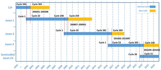
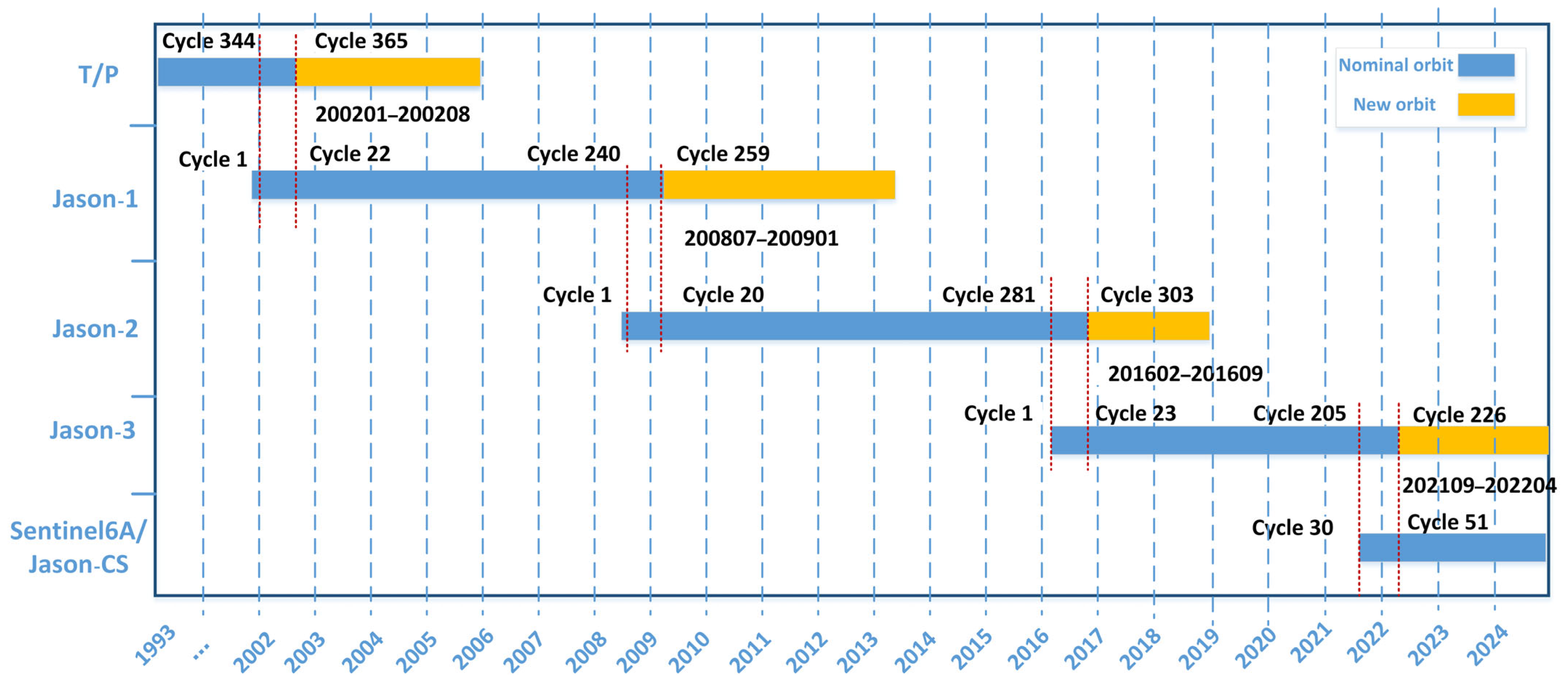
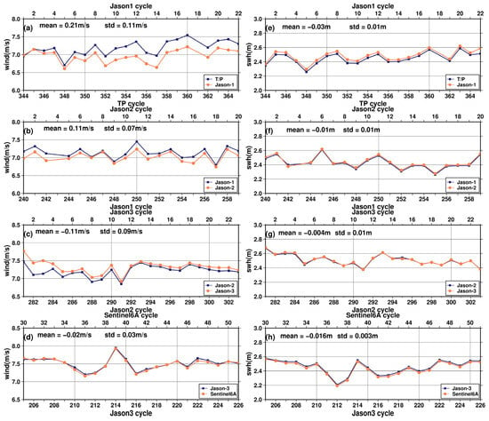
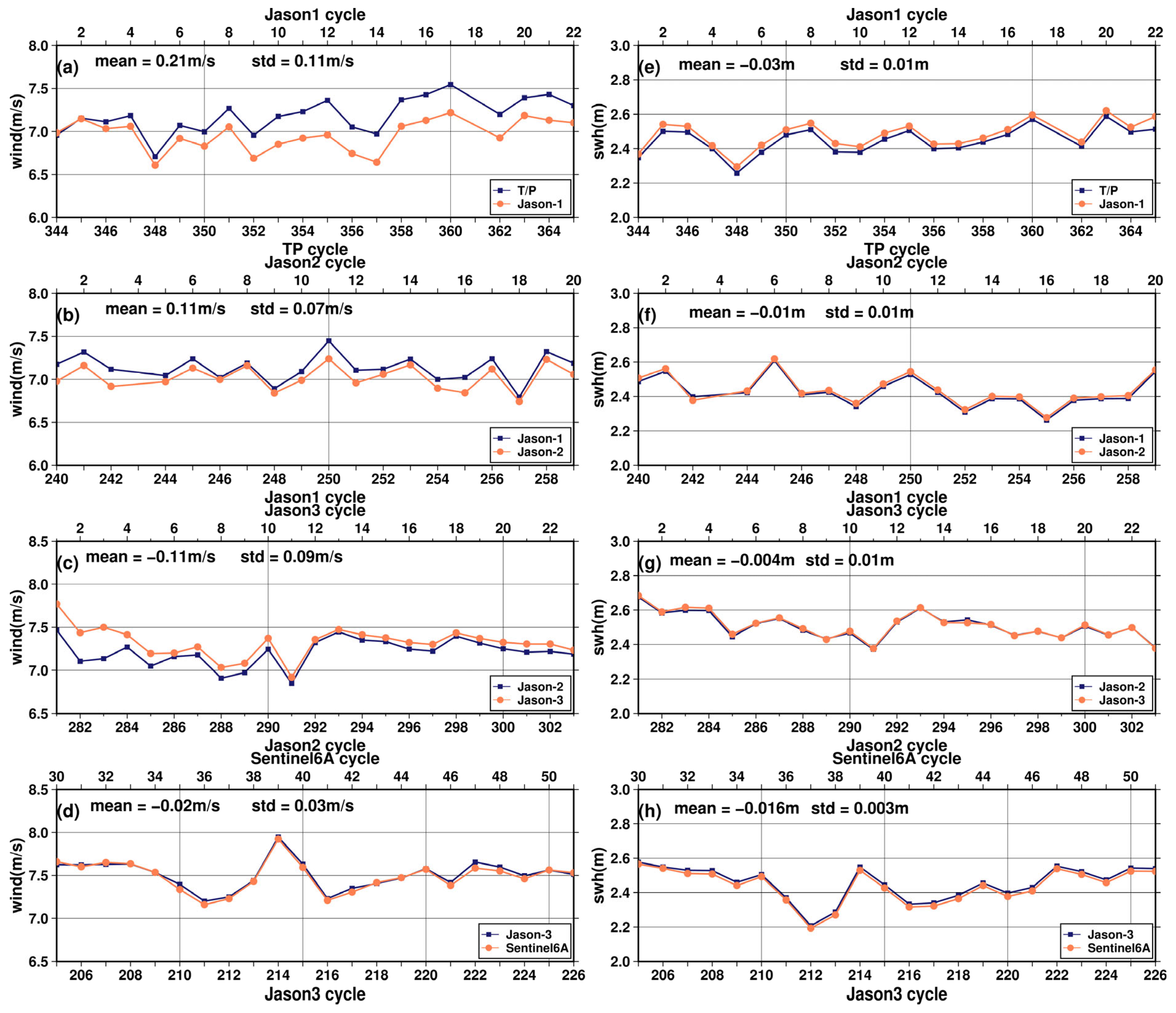
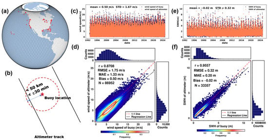
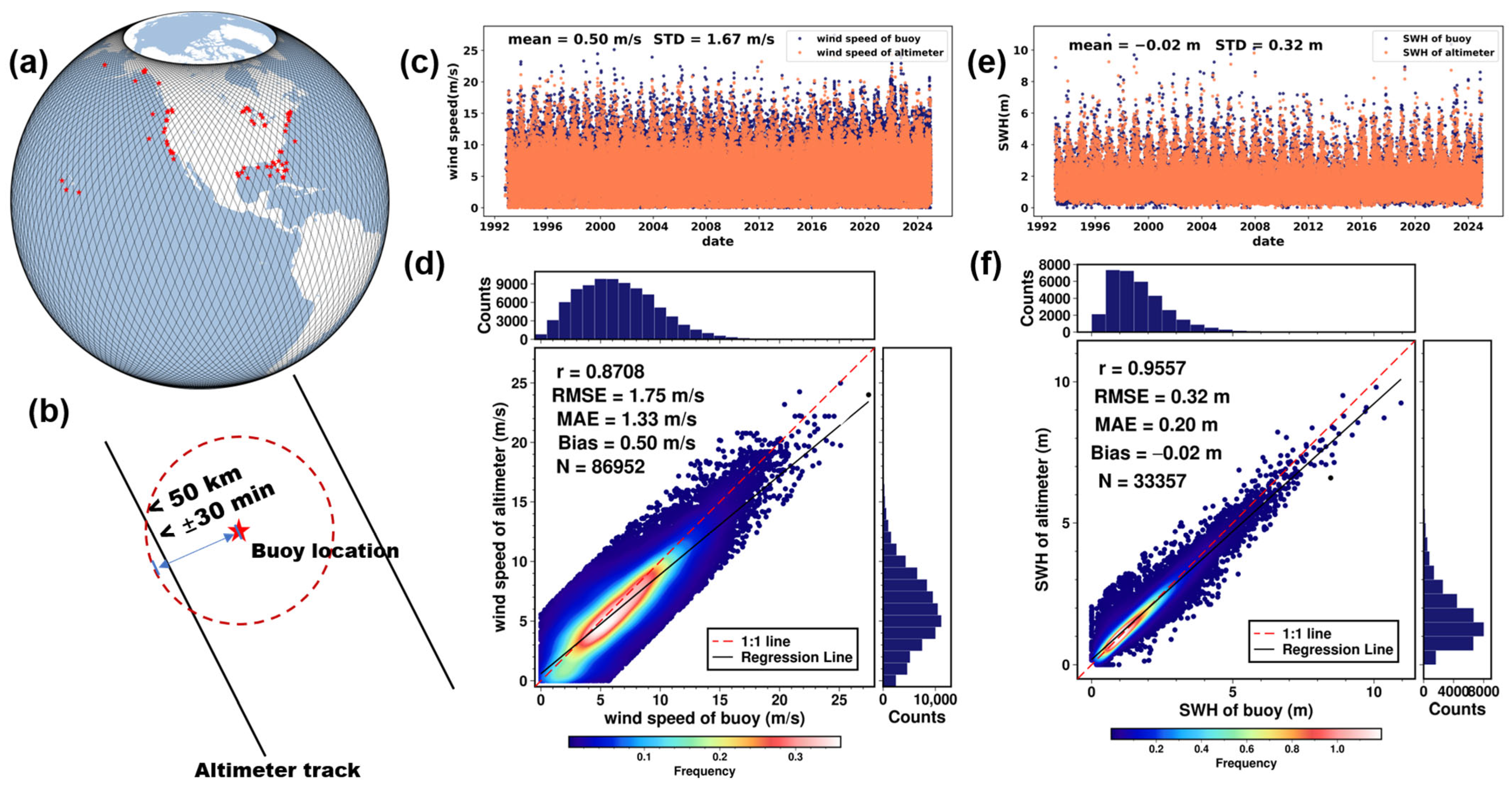
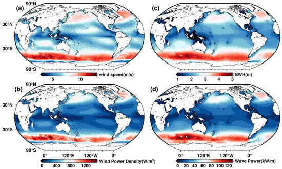
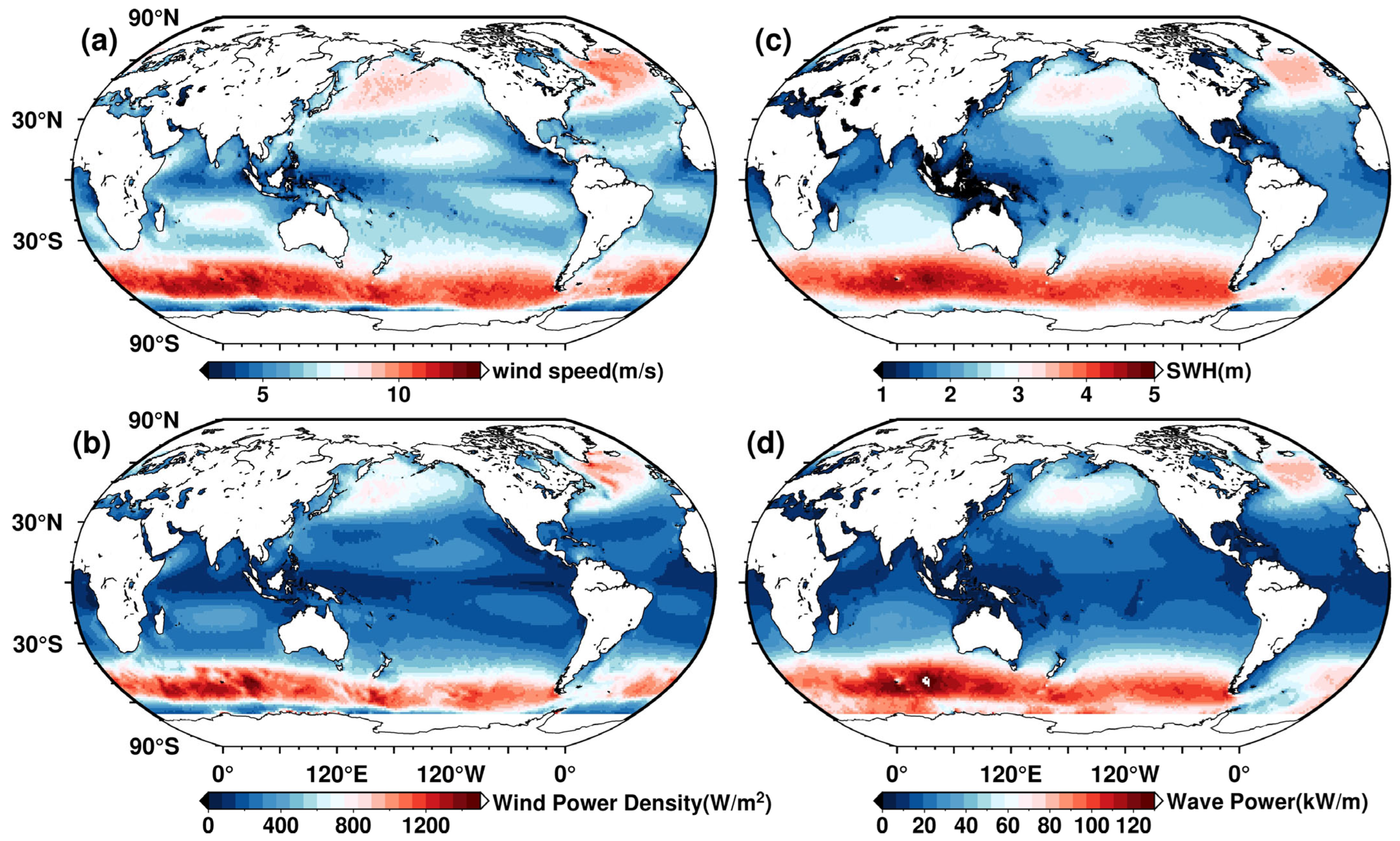
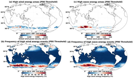
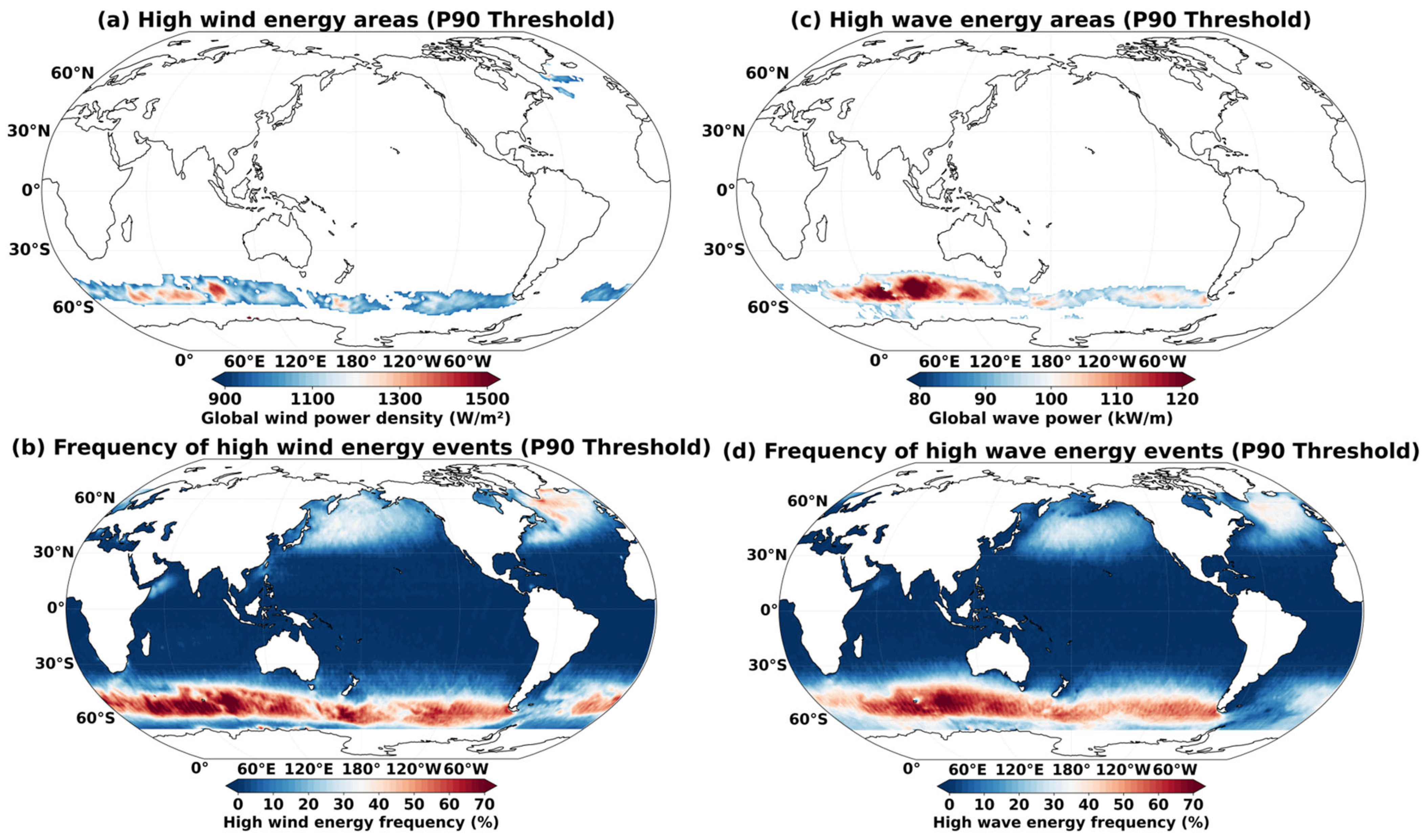
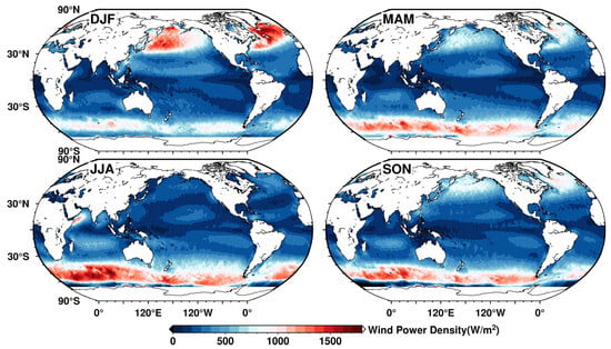
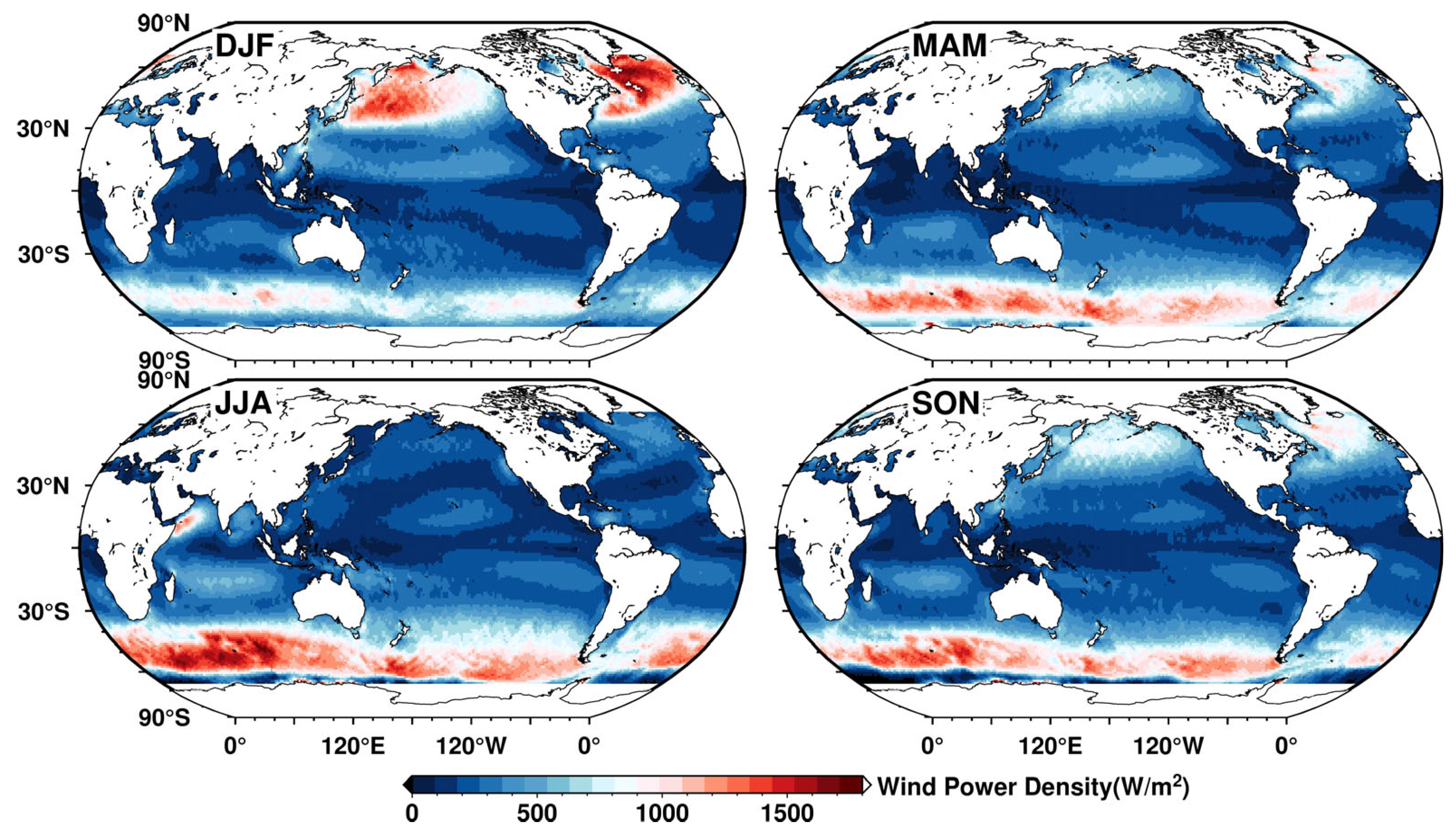
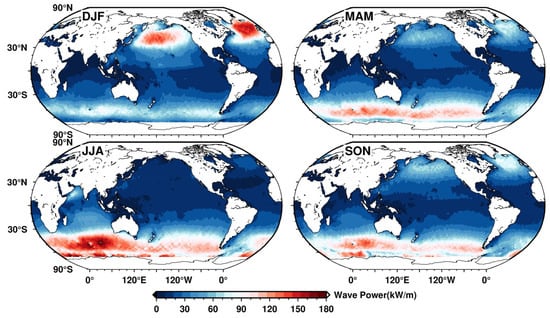
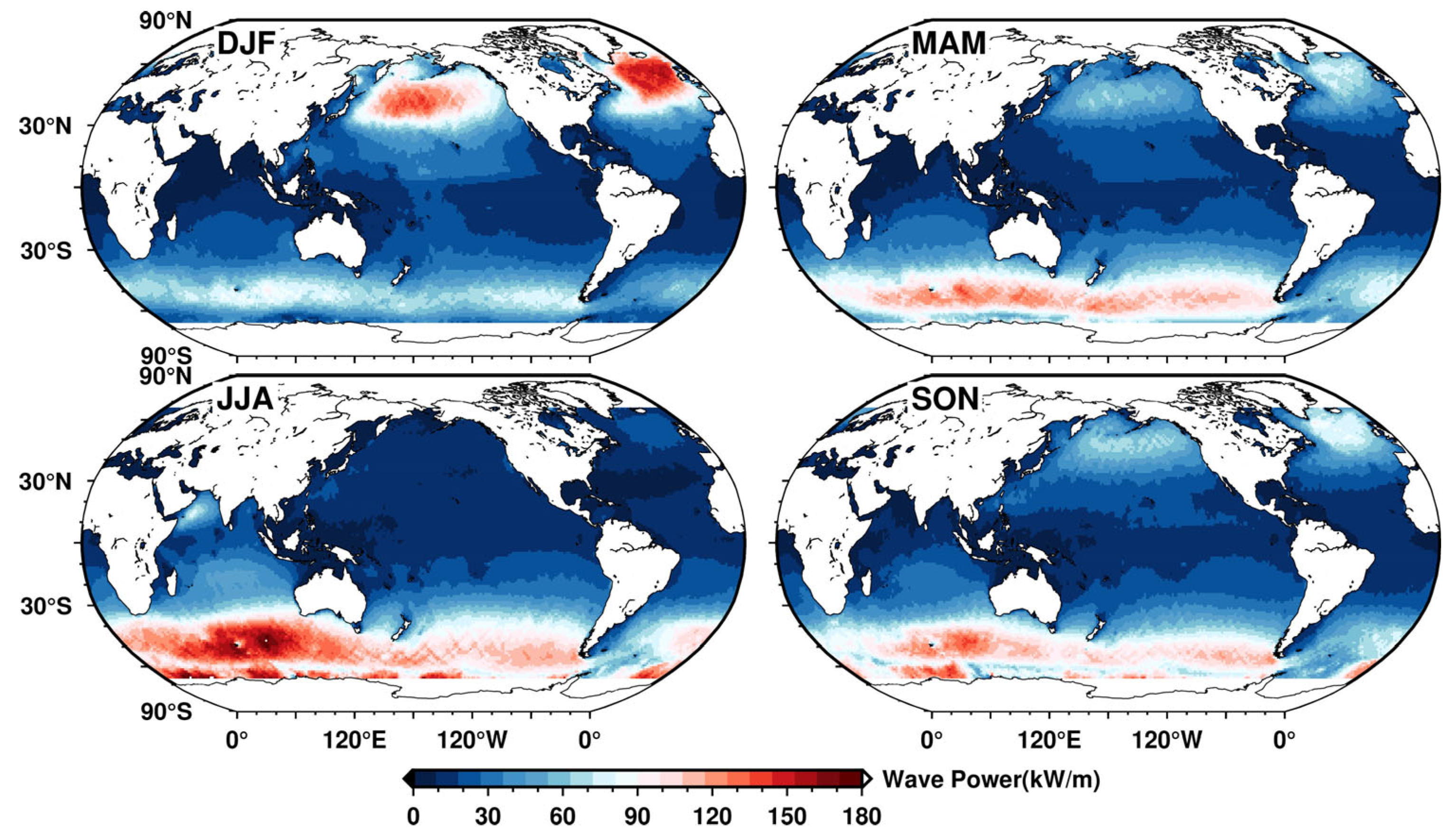
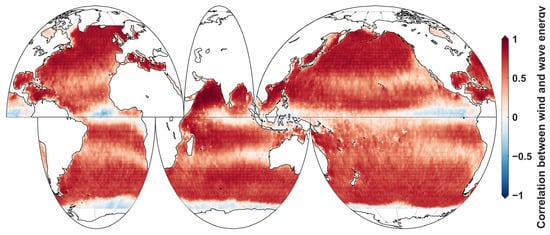
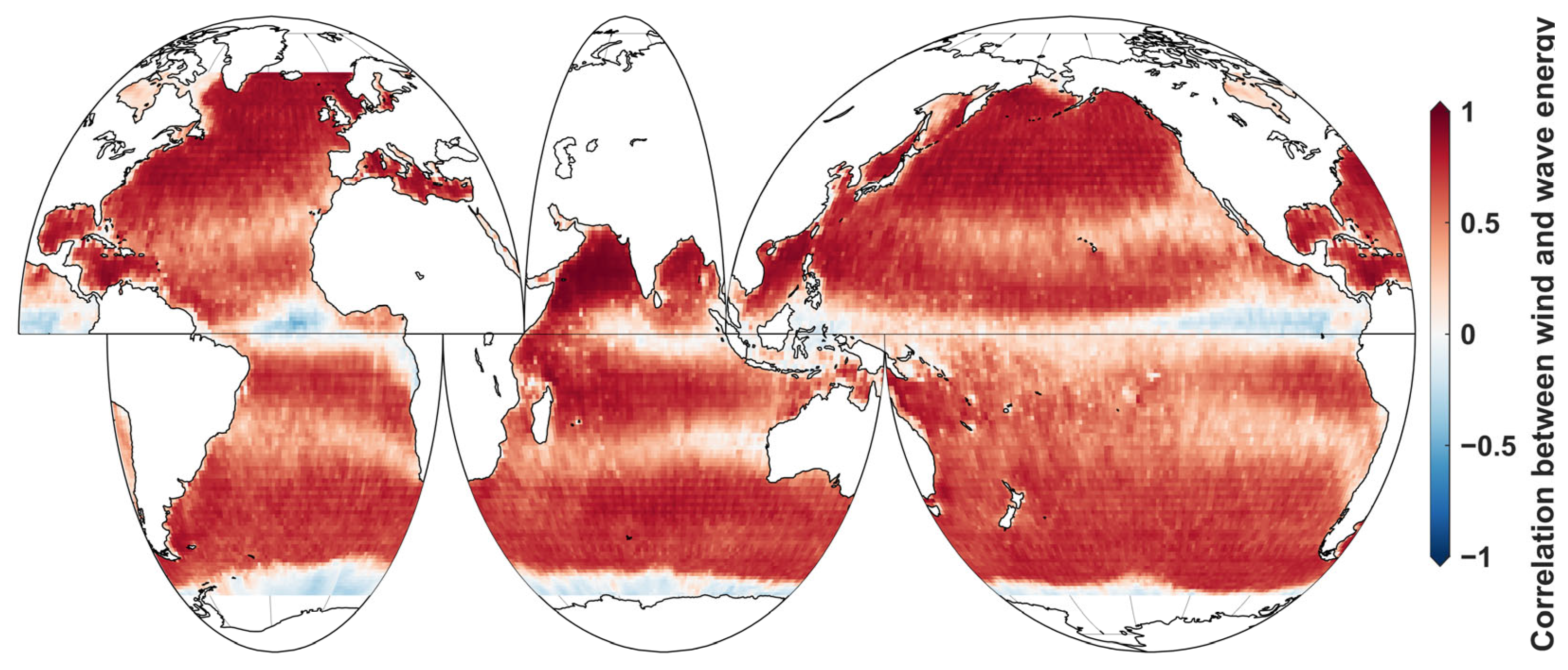
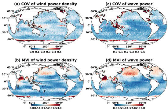
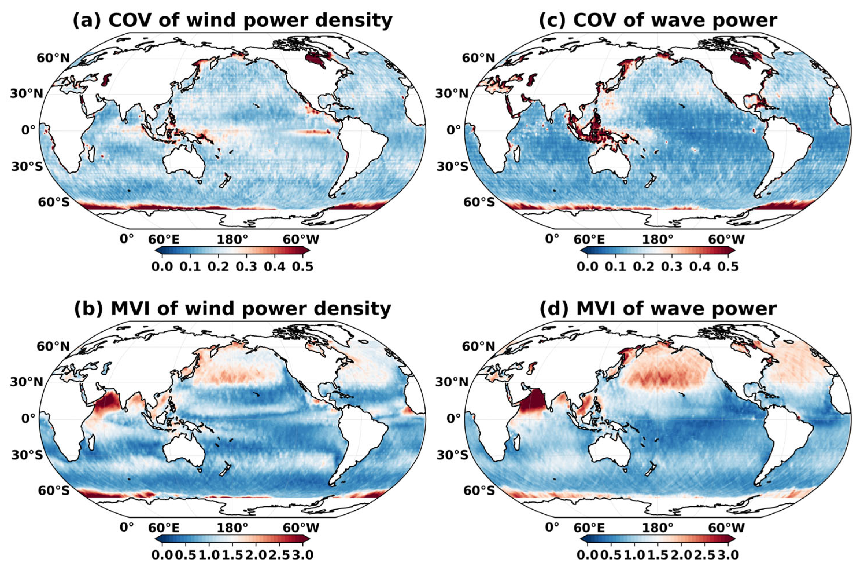
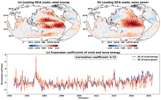
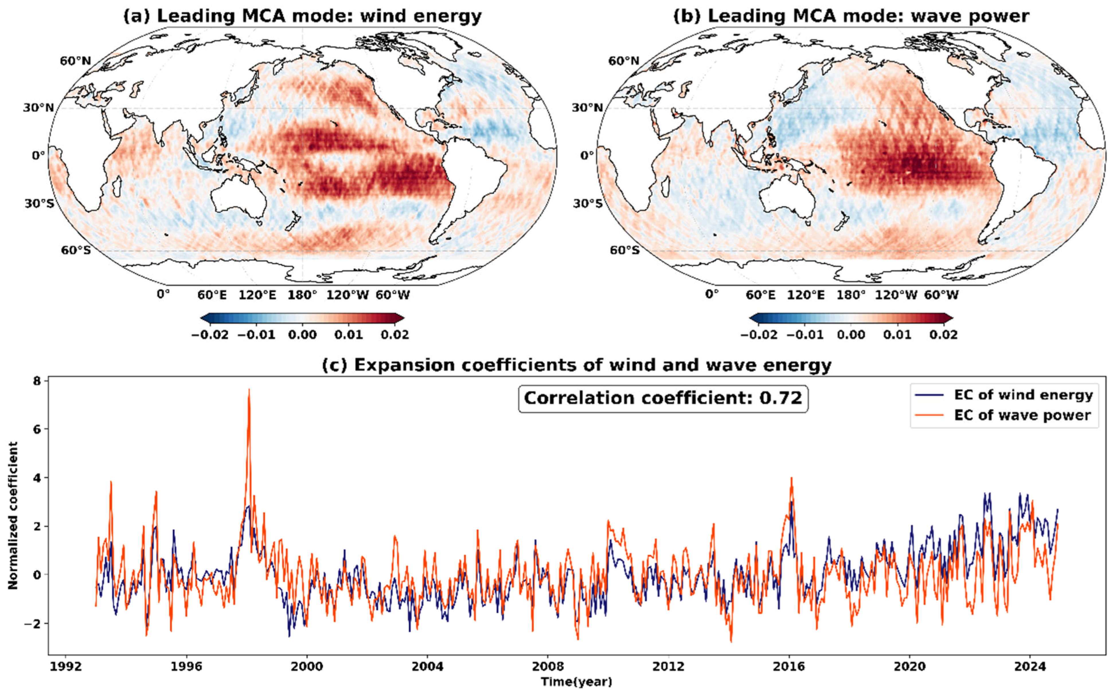
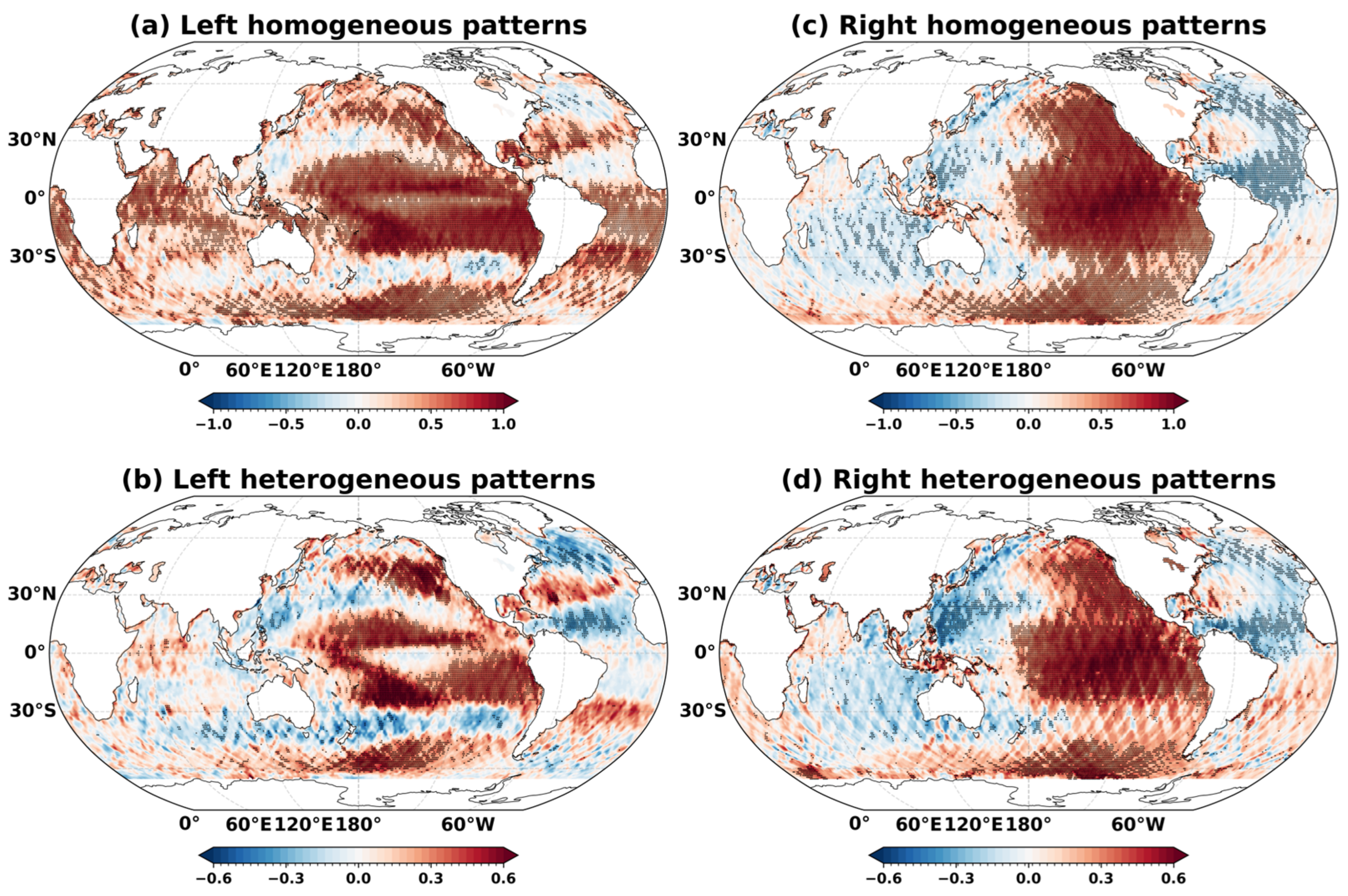
Disclaimer/Publisher’s Note: The statements, opinions and data contained in all publications are solely those of the individual author(s) and contributor(s) and not of MDPI and/or the editor(s). MDPI and/or the editor(s) disclaim responsibility for any injury to people or property resulting from any ideas, methods, instructions or products referred to in the content. |
© 2026 by the authors. Licensee MDPI, Basel, Switzerland. This article is an open access article distributed under the terms and conditions of the Creative Commons Attribution (CC BY) license.