Net-Energy Path Planning for Unmanned Surface Vehicles in Time-Varying Wind-Solar Energy Fields

Abstract

To address the spatiotemporal variations of wind and solar resources, the energy consumption of unmanned surface vehicles (USVs), and island–reef obstacle constraints in offshore mobile energy resupply missions, this paper proposes a dynamic multi-objective path planning method oriented toward net energy. A fine-grained obstacle grid is constructed based on satellite imagery, and an hourly ERA5-based wind–solar energy field is constructed independently of the ANP suitability assessment. Energy harvesting, propulsion energy consumption, and onboard base loads are incorporated into a unified energy balance model, with net energy and voyage distance as the optimization objectives. A receding-horizon ME-DMOEA is employed to dynamically optimize the remaining path, and dual-scale grids are used for obstacle detection and local repair. After fine-grid path repair, ME-DMOEA achieved net-energy improvements of 35.83 Wh in S1 and 82.82 Wh in S2 relative to the implemented four-neighbor A* baseline. In 30 paired runs, ME-DMOEA and NSGA-II tied in S1, while ME-DMOEA achieved higher mean net energy in S2 under both tested ERA5 environments. The rolling ON/OFF net-energy difference was not statistically significant. These simulations support net-energy-aware planning under modeled static-obstacle and terminal constraints, without establishing COLREGs-compliant collision avoidance or real-vessel performance.

1. Introduction

As offshore aquaculture, environmental monitoring, and maritime transportation tasks progressively move toward unmanned and electrified operation, the endurance and energy resupply issues of unmanned surface vehicles (USVs) have become increasingly prominent. Returning to port for charging increases non-operational voyage distance and mission interruption time, whereas fixed offshore energy supply facilities are constrained by construction costs and service coverage [1]. USVs equipped with photovoltaic and wind energy harvesting devices can acquire renewable energy during navigation, offering a feasible approach for mobile energy resupply [2]. However, wind and solar energy exhibit pronounced spatiotemporal variability; sailing toward high-energy regions also increases voyage distance and propulsion energy consumption, so a higher amount of energy harvested does not necessarily correspond to a higher final energy surplus [3,4,5].

Existing studies have investigated renewable-energy marine platforms, environmental effects on USV navigation, and multi-objective route optimization. These developments motivate a task-oriented formulation for mobile energy resupply that evaluates route-dependent renewable-energy gains after subtracting the supplying USV’s propulsion consumption and onboard base loads. This study considers the joint optimization of net energy and voyage distance under time-varying wind–solar availability, a prescribed rendezvous requirement, and island–reef obstacles. The focus is on the potential energy surplus at arrival; the physical inter-vessel energy-transfer process is outside the present model.

To address the above issues, this paper develops a receding-horizon net-energy path planning framework. First, a dual-scale environment model is constructed using a 1 km energy planning grid and a 100 m obstacle grid. Second, wind–solar energy harvesting, propulsion energy consumption, and onboard base loads are unified into an energy balance model, with net energy and voyage distance adopted as the two optimization objectives. Finally, ME-DMOEA is employed to re-optimize the remaining path at each receding-horizon step, and fine-grained collision detection and local repair are performed on the actually executed segment, thereby coordinating time-varying energy utilization, navigation efficiency, and terminal reachability. The present evaluation focuses on static island–reef obstacles in numerical simulations; collision avoidance involving moving vessels, COLREGs compliance, and real-vessel operations remain outside the validated scope.

2. Related Work

2.1. Marine New-Energy Unmanned Platforms and Mobile Energy Replenishment

New-energy-powered unmanned platforms have shown considerable potential for long-endurance autonomous marine operations. Minak reviewed solar-powered boats and discussed photovoltaic applications in maritime drones, providing a technological basis for renewable-energy marine platforms [6]. Yuan et al. demonstrated a photovoltaic unmanned vessel for mobile monitoring, fixed-point sampling, and dissolved-oxygen enrichment [7]. Marini et al. proposed the ENDURUNS architecture, in which a USV equipped with photovoltaic panels, hydrogen fuel cells, and batteries supports a hybrid AUV and is designed to transfer power to it through docking [8]. Davis et al. subsequently developed and field-tested a robotic path-planning system for aquaculture water-quality monitoring [9]. Jia et al. developed a dynamic Dijkstra-based planner that accounts for wind-energy capture and onboard energy consumption in time-varying wind fields, enabling route selection according to net energy consumption [10].

These studies provide a basis for renewable-energy marine platforms, autonomous monitoring, and inter-vehicle energy support. Building on this background, the present study examines how a supplying USV can plan its route to a designated rendezvous while balancing combined wind–solar harvesting against its own energy consumption. The resulting net-energy balance is used to evaluate the potential for external resupply.

2.2. Path Planning of Unmanned Surface Vehicles in Dynamic Environments

USV path-planning research has gradually expanded from static shortest-path search towards dynamic planning that considers environmental disturbances, energy consumption, and mission constraints, as summarised by Xing et al. [11]. Niu et al. investigated efficient path search, energy-consumption minimisation, and energy-efficient planning in spatially and temporally varying environments [12,13,14]. Gu et al. incorporated wind and current effects into USV motion planning [15]. Yuan et al. proposed a utility dynamic window approach that incorporates wind and wave effects and COLREGs requirements into local collision avoidance [16]. Luo et al. further proposed an energy-efficient method for time-varying maritime environments [17].

Recent research on maritime autonomous surface ships (MASS) further emphasizes COLREGs compliance and collision avoidance in practical navigation. Namgung et al. reviewed MASS path-planning and collision-avoidance technologies, including the Navigation-GPT framework [18], while Namgung investigated COLREGs-compliant local route planning based on ship domains and velocity obstacles [19]. These safety-oriented studies complement the energy-aware route optimization considered in this paper.

Related studies have also addressed task continuity and dynamic replanning. MahmoudZadeh et al. developed an uninterrupted planning system for multi-USV sampling missions in cluttered environments [20], and Zhang et al. considered time-varying wind and current in dynamic energy-efficient planning [21]. Chowdhury et al. formulated multi-objective path planning as a Markov decision process and used GPU acceleration to evaluate trade-offs between travel time and net energy consumption, including a solar-energy-harvesting surface-vehicle scenario in stochastic dynamic flows [22]. Sudha et al. investigated coverage path planning for environmental monitoring [23]. Existing studies therefore address environmental disturbances, collision avoidance, energy-efficient navigation, and energy-harvesting-aware route optimisation. The present work brings combined wind–solar harvesting, distance-dependent propulsion consumption, and onboard base loads into a receding-horizon model for a mobile energy-resupply mission. Net energy and voyage distance are optimised jointly subject to a prescribed terminal requirement, while a dual-scale grid supports energy evaluation and fine-scale obstacle handling.

2.3. Dynamic Multi-Objective Optimisation

Dynamic multi-objective optimisation provides a suitable basis for balancing energy gain, voyage length, and rendezvous-time constraints under changing environments. Farina et al. established a classical framework for dynamic multi-objective optimisation problems [24], and Jiang et al. reviewed major response mechanisms including diversity maintenance, memory, prediction, and transfer [25]. Subsequent studies developed more specialised dynamic-response strategies. Wu et al. proposed a dynamic response mechanism [26], while Zheng et al. introduced prediction based on decision-variable analysis [27]. Chen et al. developed an adaptive response-mechanism selection strategy [28], and Wang et al. combined particle-swarm prediction with prediction adjustment [29].

More recent work has focused on improving prediction, diversity, and constrained optimisation. Wu et al. developed a prediction-based dynamic multi-objective evolutionary algorithm [30], Peng et al. proposed hybrid environmental-change responses [31], and Gong et al. introduced prediction and weak cooperative co-evolution for dynamic constrained multi-objective optimisation [32]. Therefore, dynamic multi-objective optimisation methods provide an algorithmic foundation for handling the energy–voyage trade-off under time-varying environments, but they cannot directly resolve the energy balance, rendezvous time, and island–reef obstacle avoidance issues involved in the task of this paper. Accordingly, this paper integrates rolling dynamic optimization with the mobile energy resupply task model, re-solving the remaining path after each environment update.

3. Research Areas and Environmental Modelling

3.1. Research Areas and Detailed Obstacle Maps

To evaluate the proposed path planning method in a real sea area with complex geographical constraints, this paper selects a nearshore island–reef region in the Bohai Sea as the study area. This region contains multiple islands, irregular coastlines, and land areas, thereby providing a representative test environment for path feasibility and local obstacle avoidance. Based on the longitude and latitude range and the actual scale of the study area, a unified spatial coordinate system is established using a local planar approximation, with a study scope of approximately 56 km in the east–west direction and 45 km in the north–south direction. The selected study area is a subregion of the larger $56\mathrm{km}\times 70\mathrm{km}$ environmental-data domain, which is retained in the simulation for consistent spatial indexing.

First, the satellite remote sensing imagery of the study area is cropped, converted to grayscale, and segmented by thresholding; subsequently, morphological closing operations and hole filling are applied, and residual boundary discontinuities and local misclassifications are eliminated through manual correction. The resulting water–land binary image is discretized into $450\times 560$ fine grids, with each grid corresponding to an actual area of approximately $100\mathrm{m}\times 100\mathrm{m}$, where obstacle grids are denoted as 1 and navigable grids as 0. Considering the USV dimensions, positioning errors, and track-following errors, navigation safety is addressed through fine-resolution obstacle verification and local breadth-first search (BFS) repair. No additional uniform obstacle inflation is applied to the 1 km planning grid.

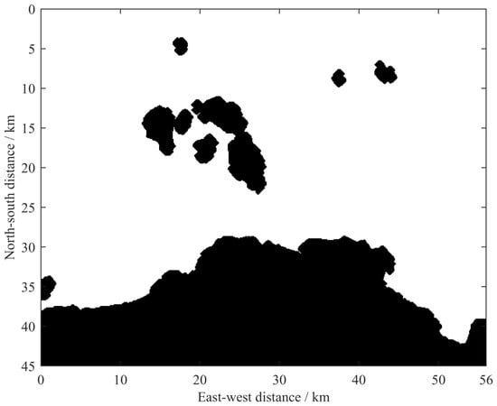
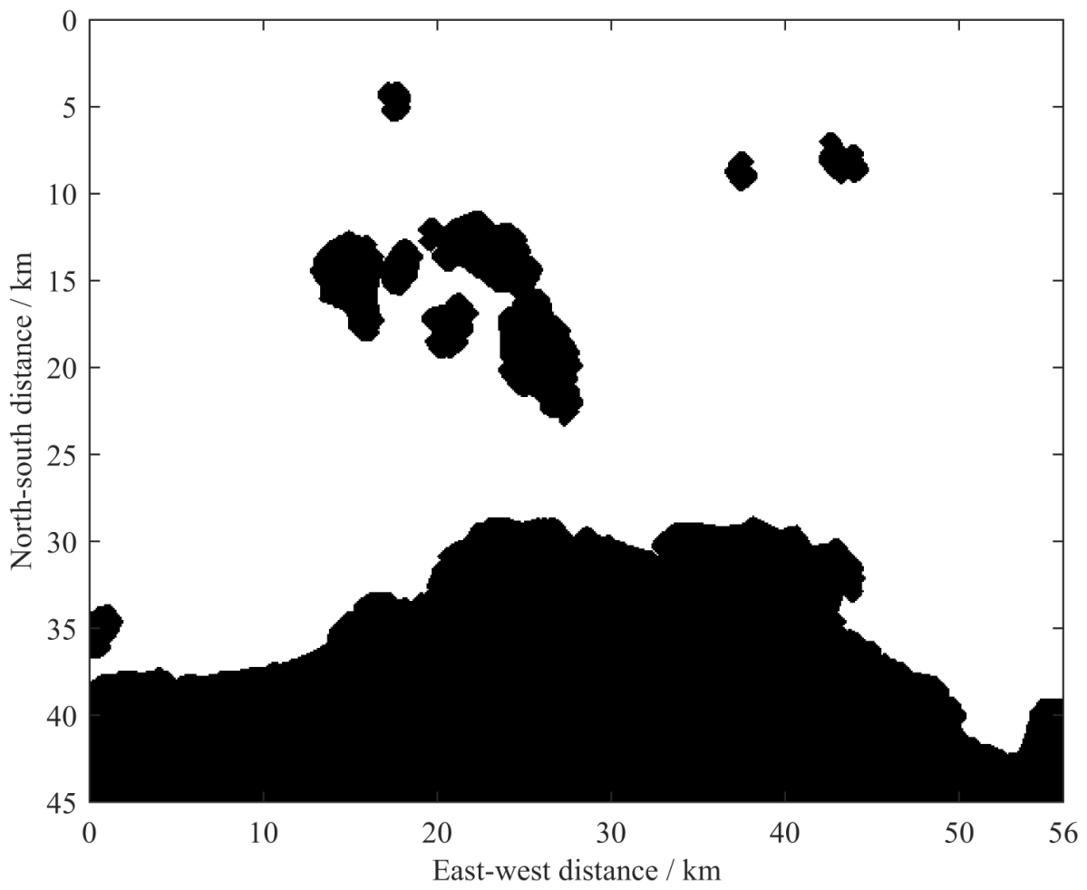
The processed target sea area occupies the grid as shown in Figure 1, with the map retaining the spatial contours of major islands, coastlines, and southern land regions, providing a spatial basis for subsequent energy grid mapping and unmanned vessel route planning.

Figure 1. Research sea areas and occupy grid maps.

Since rolling optimization requires repeatedly evaluating a large number of candidate paths at multiple time instants, performing the entire multi-objective search directly on the 100 m grid would significantly increase the computational burden of path decoding and collision detection. Therefore, this paper adopts a dual-scale spatial representation: the 1 km grid is used for dynamic energy evaluation and multi-objective path search, whereas the 100 m grid is used only for collision detection and local repair of the actually executed segment. This design controls the search scale while preserving the fine geometric constraints near islands and coastlines.

3.2. Construction of Dynamic Scenic Energy Sites

3.2.1. Energy Suitability Assessment Based on ANP

The availability of wind and solar energy depends not only on resource intensity but is also influenced by factors such as cloud cover, wind direction stability, ambient temperature, and sea state, among which certain correlations exist. For example, cloud cover affects the effective solar irradiance, ambient temperature affects the operating condition of photovoltaic modules, and waves affect platform stability and energy harvesting conditions. Therefore, this paper adopts the Analytic Network Process (ANP) to evaluate the suitability of the renewable energy harvesting environment at different sea-area locations.

The ANP evaluation system consists of a goal layer, a criterion layer, and a sub-criterion layer. The goal layer represents the comprehensive energy harvesting suitability of the mobile energy resupply USV; the criterion layer includes the photovoltaic energy harvesting condition, the wind energy harvesting condition, and the platform operation and energy storage adaptability; the sub-criterion layer comprises indicators such as solar irradiance, wind speed, wind direction stability, cloud cover, temperature, wave, and energy storage temperature.

Pairwise comparisons use the Saaty 1–9 scale. Local priorities derived from the comparison matrices are combined through the ANP supermatrix procedure to obtain the six comprehensive factor weights in Table 1, rounded to four decimal places. The ANP weighting procedure is used to characterize the relative importance of environmental suitability factors rather than to determine the physical wind–solar energy harvested by the USV.

Table 1. Comprehensive weights of main environmental factors by ANP.

Rank	Environmental Factor	Comprehensive Weight	Function
1	Wind speed	0.3769	Primary driving factor of wind energy resources
2	Cloud cover	0.2226	Correction of available photovoltaic irradiance utilization
3	Wind direction stability	0.1528	Reflect the continuity of wind energy utilization
4	2 m air temperature/temperature proxy	0.1337	Environmental correction for photovoltaic and temperature
5	Wave effect	0.0979	Platform disturbance and risk suppression
6	Energy storage battery temperature	0.0159	Operating environment correction of energy storage

From Table 1, it can be seen that wind speed has the highest weight, followed by cloud cover and wind direction stability, indicating that the assessment of an energy site needs to consider resource intensity, availability and stability simultaneously.

To eliminate dimensional differences, each environmental indicator is mapped to the [0, 1] interval, and combined with ANP weights, the comprehensive suitability of new energy can be expressed as:

$$\Phi (i,j,t)={\displaystyle \sum _{k=1}^K}{\omega }_k{S}_k(i,j,t)$$

(1)

where ${\omega }_k$ is the ANP comprehensive weight of the k-th environmental factor, $S_k(i,j,t)$ denotes the suitability of this factor at time t and grid $(i,j)$, and $\Phi (i,j,t)\in [0,1]$ represents the comprehensive energy suitability. A larger value indicates that the location is more favorable for the mobile energy-supplying unmanned surface vehicle to carry out wind and solar energy harvesting.

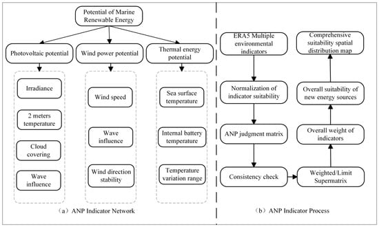
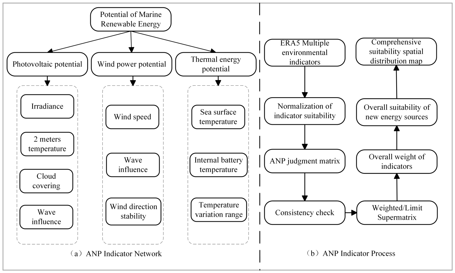
Figure 2 summarizes the ANP procedure: environmental-indicator input, suitability normalization, judgment matrices and consistency testing, weight calculation, and spatial assessment. The dimensionless index $\Phi (i,j,t)$ characterizes the combined environmental influences on wind–solar harvesting conditions. The index and its weights serve only as auxiliary environmental assessment and do not enter the path-optimization objectives. Physical harvestable energy for the energy balance is calculated independently from ERA5 data and wind and photovoltaic generation models.

Figure 2. ANP energy index network and comprehensive suitability assessment process for new energy.

3.2.2. Construction of a Time-Varying Renewable-Energy Field

The net-energy model requires physical energy quantities, estimated from hourly ERA5 data and onboard wind and photovoltaic generation models during navigation.

Based on hourly wind speed, solar irradiance, ambient temperature, and the characteristics of the onboard wind and photovoltaic generation devices, the harvestable wind and photovoltaic energy within each 1 km planning grid are calculated separately. The total renewable energy available in grid $(i,j)$ during time interval t is defined as:

$$\begin{array}{cc}\hfill E(i,j,t)& =E_{\mathrm{PV}}(i,j,t)+E_{\mathrm{wind}}(i,j,t)\hfill \\ \hfill & =3.1Gclip\left\{0.16\left[1-0.005(T-25)\right],0,1\right\}\Delta t\hfill \\ \hfill & +\min \left[1000,{\displaystyle \frac{1}{2}}\rho \pi {\left({\displaystyle \frac{D}{2}}\right)}^2{C}_p{\eta }_g{\left(u_{10}^2+v_{10}^2\right)}^{3/2}\right]\Delta t\hfill \end{array}$$

(2)

where $E_{\mathrm{PV}}(i,j,t)$ and $E_{\mathrm{wind}}(i,j,t)$ denote the photovoltaic and wind energy harvested within grid $(i,j)$ during the corresponding one-hour interval, respectively.

Here, G is the hourly mean solar irradiance ($\mathrm{W}/{\mathrm{m}}^2$) derived from ERA5 ssrd, T is the ERA5 2 m air temperature in °C, and $\Delta t=1$ h; $u_{10}$ and $v_{10}$ are the ERA5 10 m wind components. The operator $clip(x,0,1)$ limits x to the interval $[0,1]$. The photovoltaic model uses a panel area of $3.1{\mathrm{m}}^2$, a reference efficiency of 0.16, a temperature coefficient of $-0.005{\mathrm{K}}^{-1}$, and a reference temperature of 25 °C. In the wind model, $\rho =1.225\mathrm{kg}/{\mathrm{m}}^3$, $D=0.9\mathrm{m}$, $C_p=0.30$, and ${\eta }_g=0.30$ denote the air density, rotor diameter, power coefficient, and generator efficiency, respectively, with a rated-power limit of $1000\mathrm{W}$. The 2 m air temperature is used as a temperature proxy for the photovoltaic model.

The study area is discretized into a $45\times 56$ energy-planning grid at a spatial resolution of approximately 1 km. Hourly ERA5 environmental variables are mapped onto this grid. The ERA5 inputs include the 10 m wind components ($u_{10}$ and $v_{10}$), 2 m air temperature ($t_{2\mathrm{m}}$), and surface solar radiation downwards ($ssrd$). ERA5 timestamps are aligned from UTC to Beijing Time (UTC+8); air temperature is converted from kelvin to degrees Celsius, and accumulated shortwave-radiation energy is converted to mean irradiance according to its accumulation interval. Scenario S1 covers 07:00–18:00, corresponding to 12 hourly time stamps and 11 executable one-hour intervals. Scenario S2 covers 08:00–17:00, corresponding to 10 hourly time stamps and 9 executable intervals. The resulting time-varying energy fields are used as environmental inputs for the rolling-horizon path-planning experiments.

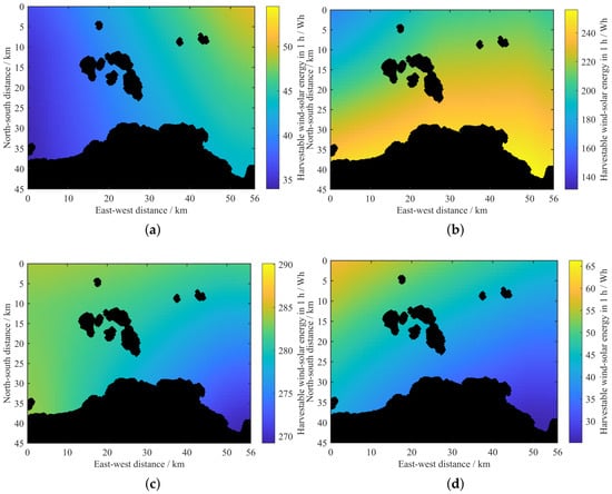
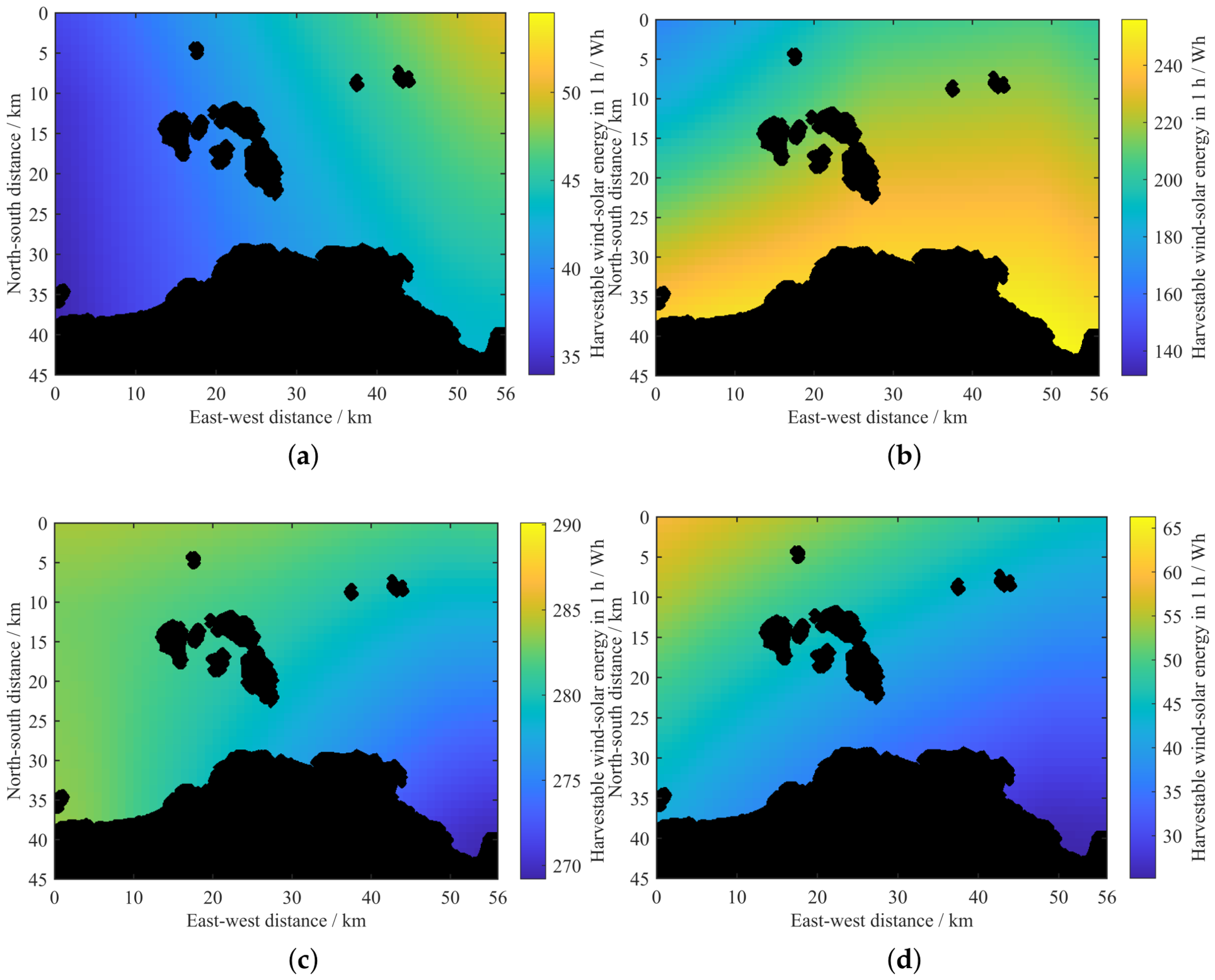
Figure 3 illustrates the renewable-energy distributions at four representative time instants. The results show that both the energy intensity and its spatial distribution vary over time, indicating that a static energy map cannot adequately represent the renewable-energy environment throughout the entire mission period. Therefore, the remaining route needs to be re-evaluated using the updated energy field at each rolling instant to adapt to temporal variations in renewable-energy availability.

Figure 3. Dynamic energy field of the typical moment target sea area. (a) 07:00. (b) 12:00. (c) 15:00. (d) 18:00.

From the perspective of path optimisation, the constructed renewable-energy field introduces a spatiotemporal dependency into route evaluation. Different candidate paths traverse different grid cells and consequently encounter different energy conditions. Furthermore, even if two candidate paths pass through the same geographic region, their harvested energy may differ because the vessel reaches that region at different times. Therefore, route evaluation depends not only on the spatial trajectory of the vessel but also on the temporal sequence of reaching each location. This spatiotemporal coupling provides the environmental basis for the rolling-horizon optimisation framework developed in this study.

3.3. Mobile Energy Replenishment Tasks and Path Representation

It is assumed that the energy-receiving vessel remains at the designated rendezvous point during the planning period, or its expected rendezvous location is known within the current planning horizon. The energy-collecting unmanned vessel departs from a given starting point and needs to reach the energy supply rendezvous point within the specified mission time limit. The planning process is updated on an hourly rolling basis: at each rolling moment, the complete remaining path is re-optimised based on the unmanned vessel’s current position, remaining mission time, and the latest energy field, but only the current control period of the selected path is executed. After execution, the unmanned vessel’s position is updated, and the optimisation problem is reconstructed at the next moment. This study focuses on the energy collection and path planning process before the rendezvous and does not involve the docking of the two vessels or the actual energy transfer process.

Let $s_t$ denote the current position of the unmanned vessel at rolling instant t, and let $H_t$ denote the remaining number of executable time intervals. The remaining candidate path can be represented as

$$P_t=\left\{p_t^0,p_t^1,\dots ,p_t^m\right\},$$

(3)

where $p_t^0=s_t$ and the final point of $P_t$ corresponds to the energy replenishment rendezvous point. The algorithm optimises the complete remaining route at the current rolling instant, whereas only the first-hour segment of the selected route is physically executed. After execution, the vessel position is updated, the remaining planning horizon is shortened, and the optimisation problem is reconstructed using the newly available energy field.

Accordingly, the proposed rolling mechanism forms a rolling feedback process of remaining path optimisation, current segment execution, state updating, and re-optimisation. The route generated at the beginning of the mission is therefore not assumed to remain optimal throughout the entire task. Unexecuted future segments can be adjusted when the energy field, vessel position, or remaining mission time changes, allowing the path to respond continuously to the time-varying environment.

The candidate path is encoded using nine control points, each containing two directional variables, row and column, resulting in a total of 18 normalised decision variables. During decoding, the normalised variables are mapped onto a 45 × 56 planning grid, and control points falling into obstacles are adjusted to the nearest navigable grid. Adjacent control points are connected via safe grid paths, ensuring that the current position remains reachable to the destination. This nine-point, 18-variable encoding is shared by all compared evolutionary optimizers; it is a fixed modeling choice rather than an independently optimized control-point count.

The control points describe the overall geometric characteristics of the candidate route rather than every individual navigation cell. After adjacent control points are connected, the resulting grid path is used to calculate the actual travel distance, energy collection, and propulsion consumption. This representation reduces the dimensionality of the decision space while preserving sufficient flexibility to generate different route geometries. At the 1 km planning resolution, adjacent control points are connected using four-neighbor BFS, which permits only horizontal and vertical movements. The A* baseline uses the same coarse-grid navigability mask and four-neighbor movement rule. For both methods, the resulting routes are subsequently checked and, where necessary, repaired on the 100 m obstacle grid using the same eight-neighbor BFS procedure. The lengths of the resulting executable paths are calculated from the Euclidean distances between consecutive fine-grid points.

The maximum sailing speed is 3 km/h, and the candidate paths are also constrained by the remaining time; if a control point prevents reaching the destination within the remaining time frame, it will no longer be retained. By incorporating reachability during path decoding, the search preferentially retains routes that preserve sufficient terminal accessibility and avoids excessive detours for short-term energy gains that would make timely arrival impossible.

3.4. Energy Balance Model

For a candidate path P, let H denote the number of executable one-hour intervals. The total renewable energy harvested along path P is calculated as:

$$E_{\mathrm{harvest}}\left(P\right)={\displaystyle \sum _{h=1}^H}{E}_h\left(P\right)$$

(4)

where $E_h\left(P\right)$ denotes the energy harvested along the executable route during hour h. To account for travel across multiple energy cells, the fine-grid route is divided into line segments. For each segment, the energy value of the 1 km cell containing its midpoint is weighted by the travel time, calculated as the segment length divided by the sailing speed of 3 km/h. Any remaining time within the hour is assigned to energy harvesting at the hourly endpoint. Thus, hourly harvested energy is accumulated according to the time spent along the route, rather than being determined solely by the endpoint cell.

In this study, propulsion energy consumption is approximated as a linear function of voyage distance using a constant distance-specific energy coefficient:

$$E_{\mathrm{prop}}\left(P\right)=e_{d}L\left(P\right)$$

(5)

where $L\left(P\right)$ is measured in kilometres and the constant coefficient $e_d=45\mathrm{Wh}/\mathrm{km}$ is a simulation reference, not a measured or calibrated parameter for a specific USV. It represents energy per unit distance, not constant propulsion power, and gives $E_{\mathrm{prop}}\left(P\right)$ in Wh. This common comparison model excludes speed-dependent propulsion efficiency, ocean currents, wave-induced resistance, and sea-state variations; its estimates are therefore not vessel-specific predictions under realistic hydrodynamic conditions.

The communication, navigation, perception, computing, control, and energy management components onboard the USV generate a continuous basic load. Assuming a hotel-load power of $P_{\mathrm{hotel}}$ and an operating duration of T, the corresponding energy consumption is calculated as:

$$E_{\mathrm{hotel}}=P_{\mathrm{hotel}}T$$

(6)

The aggregated onboard hotel-load power is assumed to remain constant at $P_{\mathrm{hotel}}=30\mathrm{W}$ throughout the prescribed mission duration. This value is a reference assumption used for numerical simulation, rather than a measured or calibrated load of a particular USV. Here, T denotes the complete mission duration in hours, including any remaining operating time after early arrival at the rendezvous point.

Accordingly, the hotel-load energy consumption is 330 Wh for the 11-h mission in Scenario S1 (07:00–18:00) and 270 Wh for the 9-h mission in Scenario S2 (08:00–17:00). Hotel-load consumption is calculated separately from propulsion energy and is included only once in the total energy balance.

The total modeled energy consumption of a candidate path consists of two separately evaluated components: propulsion energy and onboard hotel-load energy. It is therefore expressed as $E_{\mathrm{consume}}\left(P\right)=E_{\mathrm{prop}}\left(P\right)+E_{\mathrm{hotel}}$. After subtracting these two components from the renewable energy harvested during the mission, the net energy of path P is defined as:

$$E_{\mathrm{net}}\left(P\right)=E_{\mathrm{harvest}}\left(P\right)-E_{\mathrm{prop}}\left(P\right)-E_{\mathrm{hotel}}$$

(7)

Equation (7) provides the mission-level net-energy balance in Wh. Propulsion consumption depends on the voyage distance, whereas hotel-load consumption depends on the prescribed mission duration. Both components are subtracted exactly once from the harvested energy. For each scenario, the same energy-accounting rules are applied to all compared planning methods. The resulting net energy is used to assess the potential energy surplus at rendezvous, rather than the actual energy transferred to another vessel.

According to Equation (7), a route with higher renewable-energy harvesting does not necessarily achieve a larger net-energy surplus. If the vessel travels a significantly longer distance to access high-energy regions, the additional harvested energy may be lower than the corresponding increase in propulsion consumption, resulting in a reduced net-energy value. Therefore, net energy rather than gross harvested energy is selected as the primary energy objective to represent the balance between renewable-energy harvesting, vessel energy consumption, and potential energy surplus.

The rated battery capacity is 10,240 Wh, with 8192 Wh retained as a reference usable-capacity value. The present simulations do not prescribe an absolute initial state of charge (SOC) or propagate a dynamic SOC state; instead, route evaluation is based on the cumulative mission net energy defined in Equation (7). Therefore, 8192 Wh should not be interpreted as an initial SOC of 80%. The actual transferable energy would additionally depend on the initial SOC, battery safety margins, and transfer efficiency, which are outside the scope of the present model.

3.5. Multi-Objective Functions and Constraints

Path planning aims for two objectives: maximizing the net energy available for subsequent recharging and minimising the travel distance, using the Pareto dominance relation to preserve candidate solutions with different objective preferences. The composite objective vector is expressed as:

$$\min F\left(P\right)=\left[-E_{\mathrm{net}}\left(P\right),L\left(P\right)\right]$$

(8)

The two objectives may involve trade-offs depending on the spatiotemporal energy distribution and propulsion costs. Detouring towards a high-energy region may increase renewable-energy harvesting and improve the net-energy surplus, but it generally increases the voyage distance and propulsion consumption. Conversely, a purely shortest-path-oriented route may reduce propulsion expenditure but miss favourable time-varying energy regions. Instead of combining the two objectives in advance using fixed weighting coefficients, Pareto dominance is employed to retain candidate routes with different energy–distance trade-offs.

For two feasible candidate paths $P_a$ and $P_b$, $P_a$ is considered to dominate $P_b$ if it is no worse than $P_b$ in both objectives and is strictly better in at least one objective. Candidate paths that are not dominated by other feasible paths constitute the non-dominated solution set. In this manner, short-voyage solutions, high-net-energy solutions, and intermediate compromise solutions can coexist during the optimisation process.

Model constraints include start and end points, maximum distance per hour, obstacle safety, and remaining-time accessibility. Specifically, the following constraints are considered.

First, each remaining route must start from the current physical position of the unmanned vessel and terminate at the predefined energy replenishment rendezvous point. The starting point is updated after each executed segment, whereas the rendezvous point remains fixed under the task setting considered in this study.

Second, the distance travelled within each one-hour execution interval is limited by the maximum sailing speed. With a maximum speed of 3 km/h, the maximum executable distance during one rolling interval is approximately 3 km.

Third, candidate routes must remain within navigable regions. Coarse-grid paths are screened during path decoding, and the actually executed segments are further mapped onto the 100 m fine obstacle grid for collision verification.

Fourth, terminal reachability must be preserved throughout the rolling process. Let $D_t$ denote the safe remaining distance to the rendezvous point, $H_t$ the remaining number of executable intervals, and $\Delta t=1\mathrm{h}$ the interval duration. A necessary reachability condition is:

$$D_t\le v_{\max }{H}_t\Delta t,$$

(9)

where $v_{\max }$ is the maximum sailing speed. If this condition is violated, the candidate path is infeasible even if it temporarily achieves a favourable energy value.

The algorithm incorporates invalid grids, unreachable endpoints, duplicate or excessively long paths, deadlines, and terminal distances into a unified measure of constraint violations, denoted by $CV\left(P\right)$. A candidate solution is regarded as feasible only when:

$$CV\left(P\right)=0.$$

(10)

This treatment separates physical objectives from feasibility handling. Pareto dominance is primarily used to distinguish the energy–distance trade-offs among feasible solutions, whereas the magnitude of the constraint violation guides infeasible solutions towards the feasible region.

4. ME-DMOEA Path Planning Algorithm

4.1. Overall Framework of the Algorithm

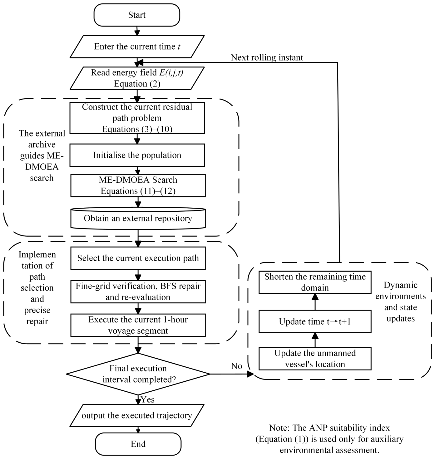
The proposed ME-DMOEA framework consists of three main stages: dynamic energy-field and task-state updating, multi-objective route optimisation, and execution-path selection with fine-grid safety repair. At each rolling instant, the current energy field, vessel position, and remaining mission time are updated. Based on these updated conditions, the residual path-planning problem is reconstructed and optimised within the remaining mission horizon.

From the perspective of the overall optimisation architecture, the proposed framework separates the dynamic planning process into an outer rolling update and an inner multi-objective optimisation procedure. The outer update describes changes in the mission environment and vessel state, including the time-varying energy field, current vessel position, and remaining mission duration. Within each rolling instant, these parameters are regarded as fixed inputs, and ME-DMOEA is applied to solve the corresponding residual path-planning problem.

This outer-update and inner-optimisation structure enables the proposed method to handle environmental variations through repeated problem reconstruction rather than continuously modifying the objective functions during a single optimisation process. Therefore, the optimisation problem remains unchanged within each rolling instant, while new optimisation problems are generated when updated environmental information and vessel states become available.

At rolling instant t, the algorithm first obtains the energy field over the remaining mission period and constructs the residual optimisation problem according to the current vessel position $s_t$. ME-DMOEA then searches for a set of feasible non-dominated routes and stores candidate solutions with different net-energy–distance trade-offs in an external archive. The execution layer selects one route from the current archive, but only the first-hour segment is implemented. Before execution, the selected segment is mapped onto the 100 m fine-resolution obstacle grid and locally repaired if a collision is detected. After execution, the updated vessel position is fed back to the next rolling instant, forming a rolling feedback process of state updating, residual-route optimisation, execution, and feedback.

The equation labels in Figure 4 link the energy-field input (Equation  (2)), residual-path formulation and constraints (Equations (3)–(10)), and particle updates (Equations (11) and (12)) to their mathematical definitions. The feedback arrow labeled “Next rolling instant” indicates that, after updating the vessel position, current time, and remaining mission horizon, the framework returns to energy-field reading for the next rolling optimization cycle.

The overall rolling framework is shown in Figure 4:

Figure 4. ME-DMOEA Overall Rolling Framework.

Figure 4. ME-DMOEA Overall Rolling Framework.

4.2. Multi-Objective Search and Particle Update

4.2.1. Candidate Evaluation and Constraint-Priority Comparison

At each rolling instant, an initial population of paths is generated randomly, and after decoding, the net energy, voyage distance, and constraint violation are calculated. The comparison of candidate solutions follows the principle of constraint prioritisation: feasible solutions are preferred over infeasible ones, feasible solutions are screened based on Pareto dominance, and among infeasible solutions, those with smaller constraint violations are prioritised.

The constraint-priority comparison avoids directly incorporating all hard constraints into the two physical objectives through large artificial penalty coefficients. Such penalty coefficients may alter the original relationship between net energy and voyage distance. By treating feasibility and objective performance separately, the physical interpretation of the two-objective formulation is preserved while constraint satisfaction remains the first priority.

The same comparison principle is also used to update the individual historical best solution of each particle. A newly generated solution replaces the previous historical best when it provides better feasibility, or when both solutions are feasible and the new solution exhibits a preferable Pareto relationship. This enables the search to retain both useful objective information and progress towards the feasible region.

4.2.2. External Archive and Leader Selection

After merging the current population with the external archive, the archive is updated through feasibility screening and non-dominated sorting; when the capacity limit is exceeded, crowding distance is used to maintain the distribution of the solution set.

The external archive is not used to retain only a single globally optimal route. Instead, it preserves a set of non-dominated solutions with different net-energy and voyage-distance characteristics at the current rolling instant. This prevents the search from concentrating prematurely on a single objective preference and provides several feasible alternatives for the subsequent execution decision. The archive leader used during particle updates should be distinguished from the route selected for execution. After optimization, an executable plan is selected from the feasible candidate solutions, considering the net-energy–distance trade-off and the remaining mission constraints. Only the selected plan is passed to the fine-grid execution and safety-verification stage.

When the number of non-dominated solutions exceeds the archive capacity, crowding distance is used to estimate the local density in the objective space. Solutions located in relatively sparse regions are preferentially retained, thereby maintaining a distributed approximation of the Pareto front rather than allowing a large number of solutions to accumulate within a narrow objective region.

The leader solution for each particle is selected from the archive using a constraint-priority and crowding tournament. Consequently, different particles may be guided by different non-dominated archive members. Some particles may continue exploring routes with shorter voyage distances, while others are guided towards regions with larger net-energy surplus, which is consistent with the multi-objective nature of the proposed path-planning problem.

The archive is maintained only during the current rolling moment. After the vessel executes the selected segment and enters the next rolling instant, the starting position, remaining mission time, and dynamic energy environment have all changed. Therefore, a new residual optimisation problem is reconstructed rather than directly treating the previous archive as a fixed solution set for the next hour.

4.2.3. Particle Update and Search Diversity

Suppose the position and velocity of the i-th particle at generation g are $X_i^g$ and $V_i^g$, respectively. Its personal-best solution is $P{B}_i^g$, and the archive-leader solution is $L_i^g$. The velocity and position are updated as:

$$V_i^{g+1}=\omega V_i^g+c_1{r}_1\left(P{B}_i^g-X_i^g\right)+c_2{r}_2\left(L_i^g-X_i^g\right)$$

(11)

$$X_i^{g+1}={\Pi }_{[0,1]}\left(X_i^g+V_i^{g+1}\right)$$

(12)

where $\omega$ denotes the inertia weight; $c_1$ and $c_2$ are learning factors; $r_1,r_2\in [0,1]$; $\Pi$ represents the boundary projection operator.

The three components of the velocity update perform different search functions. The inertia term preserves part of the previous search direction and maintains continuity of particle movement. The individual historical-best term exploits the effective search experience accumulated by each particle, whereas the archive-leader term guides the particle towards non-dominated regions discovered by the current population. Since the leader is selected from an archive rather than represented by a single global-best solution, the update rule is suitable for a multi-objective problem in which a unique optimum generally does not exist.

To maintain the population’s search capability, some particles undergo Gaussian perturbation. The perturbation introduces small variations into the normalised decision variables and can generate new combinations of control points when the population becomes concentrated in similar regions of the decision space. All perturbed particles are still subjected to the complete path-decoding, reachability, objective-evaluation, and constraint-checking procedures, so the perturbation does not bypass the original mission and safety constraints.

After particle updates, they are re-evaluated, and the individual historical best and external archive are updated according to constraint dominance relationships. The search process consisting of leader selection, particle update, perturbation, individual-best update, and archive maintenance continues until the maximum number of iterations is reached. The current external archive is then output as the candidate solution set for the execution stage.

4.3. Phased Execution and Rolling Processes

At each rolling instant, the optimizer plans the complete remaining route from the current position to the rendezvous but executes only its first-hour segment. Early, middle, and terminal stages describe decreasing detour flexibility: ample initial time permits exploration of nearby favorable energy regions; later decisions increasingly balance harvesting with progress toward the rendezvous, while excessive terminal detours should be avoided to preserve timely arrival. These stages change neither Equation (8) nor the Pareto set. In the finalized paired experiments, staged loitering and compulsory low-speed overrides were disabled; feasibility-verified plans were retained, with hourly speed limits and terminal reachability taking priority over short-term energy gains.

Before the selected first-hour route segment is physically executed, it is mapped from the 1 km energy-planning grid onto the 100 m fine obstacle grid. Every fine-grid cell intersected by the route segment is checked for collision. If a selected segment intersects obstacle cells in the adopted fine-resolution navigability mask, a local Breadth-First Search (BFS) is used to obtain a collision-free connection through navigable cells. Whenever fine-grid repair changes the route geometry, the executable distance and net energy are recalculated using the repaired trajectory. The resulting segment must also satisfy the hourly speed limit and remaining-time terminal reachability; otherwise, it cannot be accepted as a feasible executed segment.

Since fine-grid verification and repair are applied only to the route segment that will actually be executed, it is unnecessary to conduct the complete evolutionary search at the 100 m resolution. This mechanism therefore preserves local navigation safety while avoiding the high computational cost associated with fine-grid optimisation over the entire mission horizon.

After the repaired segment is executed, the vessel position and remaining mission time are updated, and the rolling time advances to the next hour. The updated energy field, reduced remaining horizon, and new vessel position jointly define the next path-planning problem. In the finalized repeated-run protocol, the terminal segment follows the previously evaluated and feasibility-verified fine-grid execution plan. The FineDeadline safeguard verifies hourly speed compliance and safe terminal arrival without silently replacing an accepted segment with a different route. Any route modification would require renewed feasibility and energy evaluation.

Accordingly, the overall information flow of the proposed method can be summarised as follows: the dynamic environmental data determine the current spatial energy distribution; the current vessel position and remaining horizon determine the feasible residual search space; ME-DMOEA generates candidate paths with different net-energy–distance trade-offs; the execution layer selects a stage-appropriate solution; fine-grid verification converts its first segment into a physically safe executable route; and the resulting state is fed back to the next rolling instant. In this manner, renewable-energy harvesting, vessel energy consumption, voyage efficiency, terminal reachability, and local navigation safety are incorporated into a unified rolling-feedback path-planning process.

The complete rolling process is shown in Algorithm 1.

Algorithm 1 ME-DMOEA for Mobile Energy-Supplement Unmanned Surface Vehicle Path Planning

1: Input: Hourly energy cube $\mathcal{E}$, fine obstacle map $G_{\mathrm{fine}}$, start point $p_s$, end point $p_e$, population size $N_p$, maximum iteration $G_{\max }$.   2: Output: Actual safe executed path reaching the energy supplement rendezvous point and net energy statistical results.   3: Initialize current time $t=1$, current position $s_1=p_s$;   4: Read energy field of current and remaining time instants;   5: Construct the current optimization problem according to $s_t$, end point and remaining time;   6: Randomly initialize the path population;   7: Decode paths and calculate net energy, voyage distance and constraint violation;   8: Build external non-dominated archive;   9: Select leader solutions from the archive; 10: Update particle velocity and position and perform mutation; 11: Decode and re-evaluate the updated particles; update personal-best solutions and the external archive; 12: Repeat Steps 9–11 until the maximum iteration number is reached; 13: Select a feasible execution plan from the current archive; 14: Verify the selected segment on the 100 m grid and apply BFS repair if necessary; 15: Re-evaluate any repaired route and verify the hourly speed and remaining-time constraints; 16: Execute the verified first-hour segment and update the vessel position; 17: if the final execution interval is completed then 18:       Verify safe arrival at the rendezvous point within the mission deadline; 19: else 20:       Set $t\leftarrow t+1$, return to Step 4; 21: end if 22: Output the verified executed path and net-energy results.

5. Simulation Results and Discussion

5.1. Simulation Configuration

The simulation settings for Scenarios S1 and S2 and the optimization parameters are summarized in Table 2. The two scenarios differ in their starting and terminal locations and mission durations, while sharing the same vessel parameters, grid representation, and optimization settings. The main experiments use the ERA5 energy field of 15 August 2025. An additional S2 experiment uses the energy field of 30 June 2025 to assess performance under a different environmental input.

Table 2. Simulation settings and optimization parameters.

Parameter		Scenario S1	Scenario S2
Scenario-specific settings
Main ERA5 date		15 August 2025	15 August 2025
Mission period		07:00–18:00	08:00–17:00
Hourly time stamps		12	10
Execution intervals		11	9
Start grid coordinate		(20, 55)	(26, 50)
Terminal grid coordinate		(22, 36)	(19, 36)
Mission duration (h)		11	9
Hotel-load energy (Wh)		330	270
Common model and algorithm settings
Parameter	Value	Parameter	Value
Energy planning grid	$45\times 56$	Path control points	9
Fine obstacle grid	$450\times 560$	Decision variables	18
Energy grid resolution	1 km	Population size	70
Fine grid resolution	0.1 km	Archive capacity	100
Maximum speed	3 km/h	Effective archive capacity	50
Propulsion coefficient	45 Wh/km	Maximum iterations	90
Hotel-load power	30 W	Inertia weight	0.72
Rated battery capacity	10,240 Wh	Learning factors $c_1,c_2$	1.49, 1.49
Usable battery capacity	8192 Wh	Random seeds	1–30

Note: The additional environmental test uses the ERA5 energy field of 30 June 2025 under the same S2 mission settings. Random seeds 1–30 apply to the repeated stochastic experiments. The propulsion-energy coefficient of 45 Wh/km and the hotel-load power of 30 W are assumed simulation reference parameters, not vessel-specific measured or calibrated values. The battery-capacity values are reference device parameters and do not specify an initial SOC or a dynamically enforced SOC constraint.

The simulations were conducted on a Lenovo Legion Y7000 IRX9 laptop equipped with a 13th-generation Intel Core i7-13650HX processor and 24 GB of RAM, using MATLAB R2024b without explicitly enabled parallel computation. In one representative S1 run, the recorded computational times were 0.0341 s for A*, 0.2565 s for Greedy, and 68.23 s for ME-DMOEA. Under the common experimental configuration with a population size of 70 and a maximum of 90 generations, the recorded framework times for ME-DMOEA and NSGA-II were 71.27 s and 90.01 s in S1 (seed 1), and 56.18 s and 71.16 s in S2 (seed 4), respectively. These measurements include method-specific execution and evaluation procedures and therefore should not be interpreted as isolated optimizer runtimes.

5.2. Simulated Executed Path and Precise Obstacle Remediation

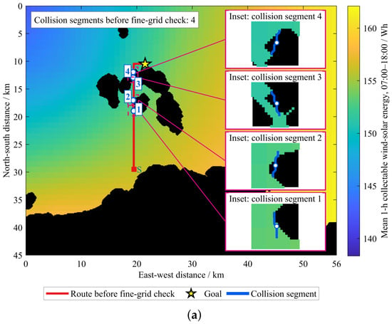
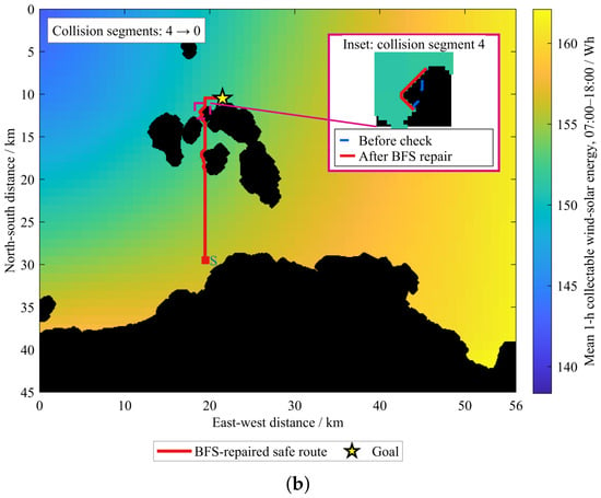
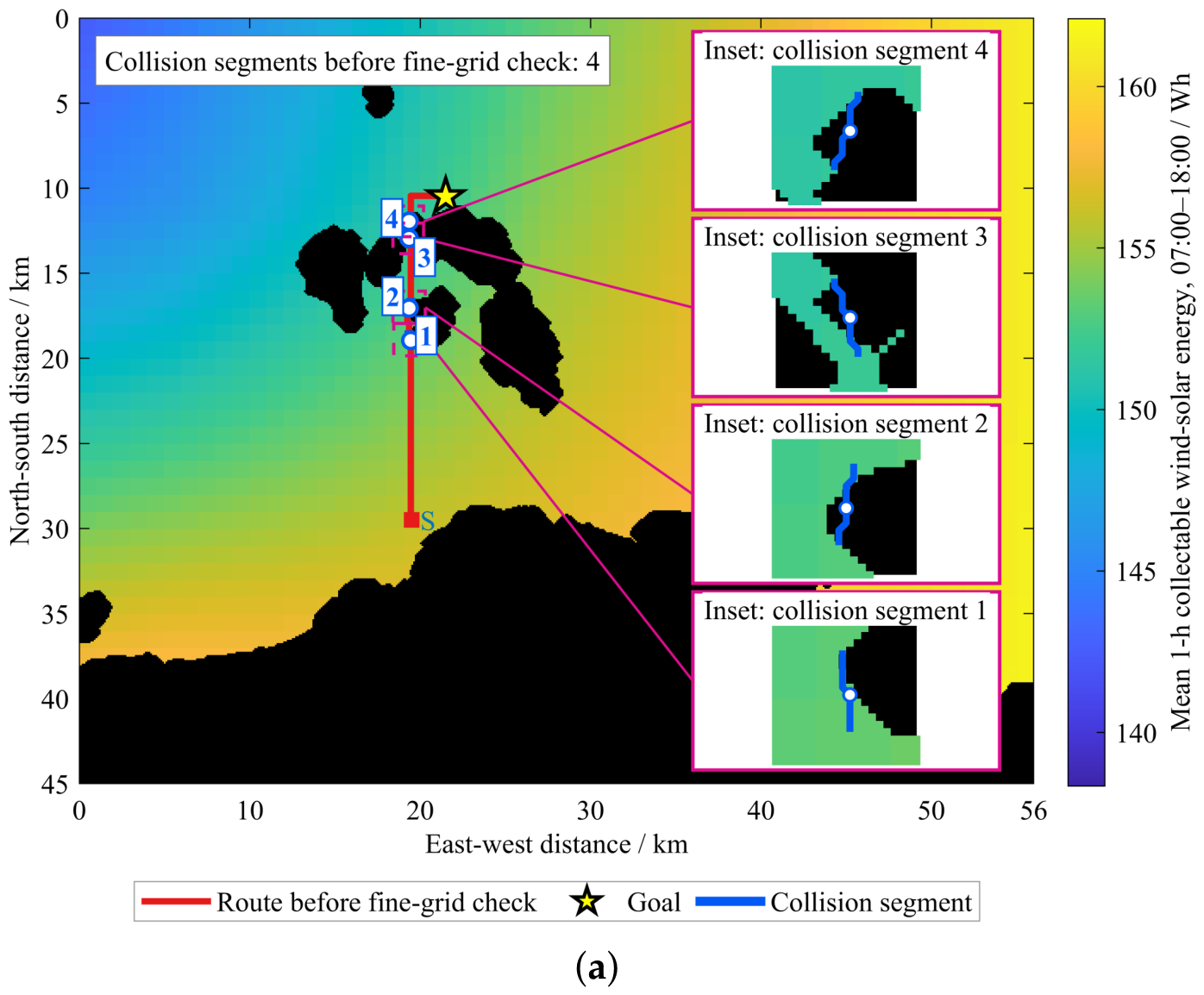
In Scenario S1, the USV travels from $(20,55)$ to $(22,36)$ during the 07:00–18:00 mission window, with 11 executable one-hour intervals. The mission time grid contains 12 hourly boundary time stamps, including the terminal instant at 18:00. The executed trajectory is updated over the mission, and the final route is verified on the 100 m obstacle grid. After mapping the coarse grid trajectory onto a 100 m fine obstacle grid, four trajectory segments intersecting obstacle areas were detected, as shown in Figure 5a.

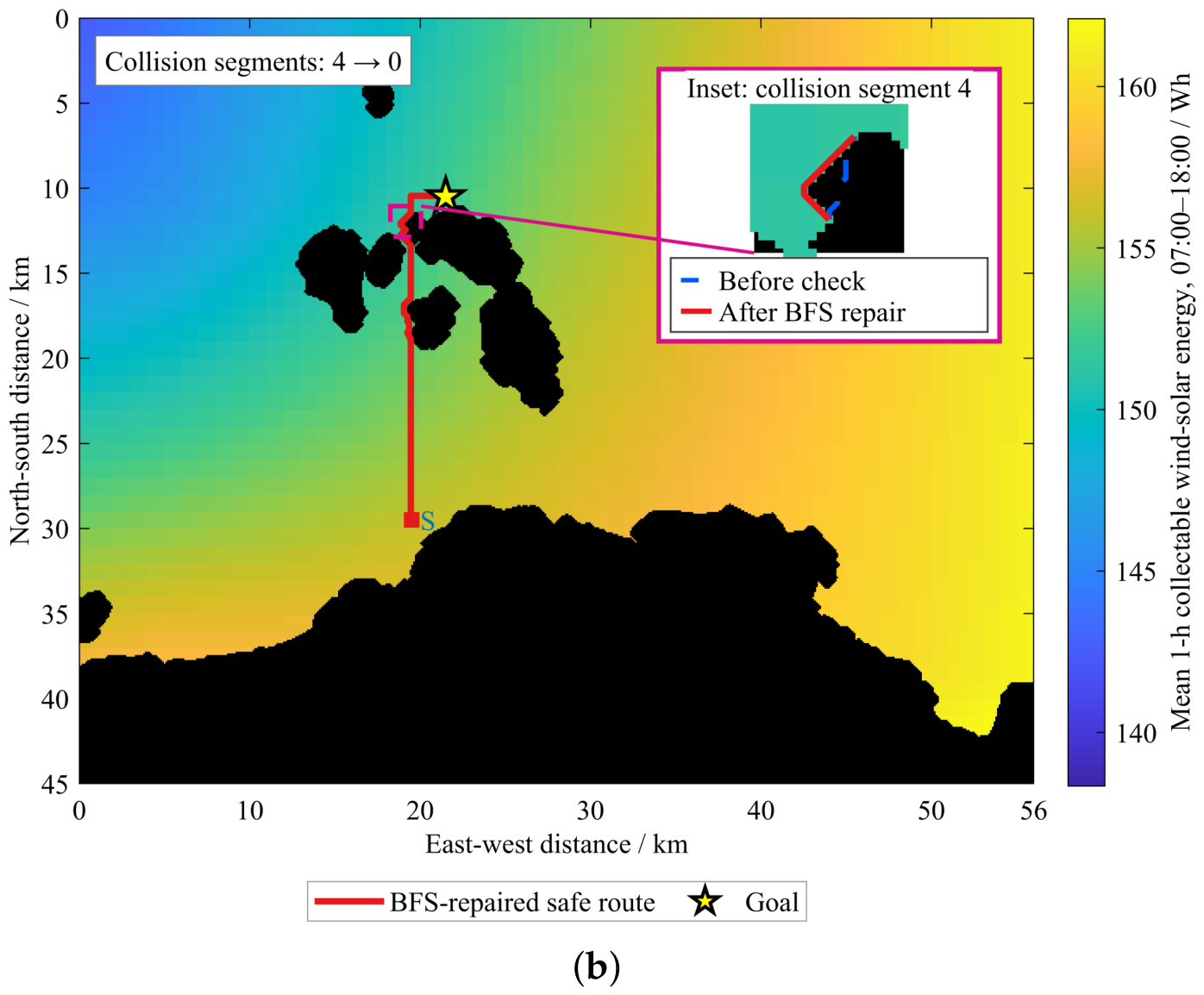
Figure 5. Fine obstacle verification and BFS repair results of the USV executed path. (a) Pre-repair path and obstacle-crossing segments on fine grid. (b) BFS-repaired safe path with local enlargement of typical segment. In both panels, “S” and the red square indicate the starting point, while the magenta boxes identify the regions shown in the enlarged insets.

After locally ensuring the safety of obstacle-crossing segments using a fine-grid BFS, all four segments were effectively repaired, leaving zero remaining obstacles, as shown in Figure 5b. The results indicate that combining a 1 km energy planning grid with a 100 m fine obstacle check can optimise the route using a time-varying energy field while ensuring that the mobile recharging unmanned vessel safely reaches the rendezvous point.

Table 3a quantifies the repair shown in Figure 5: the S1 voyage increased from 21.41 to 22.16 km. With harvested energy nearly unchanged, additional propulsion consumption reduced net energy from approximately 434.1 to 400.47 Wh. The pre-repair value is diagnostic only because the path intersects obstacles; performance comparisons use final feasible paths.

Table 3. Effects of fine-grid path repair and comparison of path-planning performance under two mission scenarios.

(a) Effects of fine-grid BFS repairon the ME-DMOEA path in Scenario S1
Metric		Before Repair			After Repair
Path length (km)		21.41			22.16
Harvested energy (Wh)		≈1727.7			1727.66
Propulsion energy (Wh)		≈963.6			997.19
Hotel-load energy (Wh)		330.00			330.00
Total consumption (Wh)		≈1293.6			1327.19
Net energy (Wh)		≈434.1			400.47
Obstacle intersections		4			0
(b) Performance comparison of the final executable paths in Scenarios S1 and S2
Scenario	Method	Path (km)	Harvest (Wh)	Propulsion (Wh)	Hotel Load (Wh)	Total (Wh)	Net (Wh)
S1	A*	22.16	1691.83	997.19	330.00	1327.19	364.64
S1	Greedy	27.42	1727.29	1233.83	330.00	1563.83	163.46
S1	ME-DMOEA	22.16	1727.66	997.19	330.00	1327.19	400.47
S2	A*	21.66	1608.89	974.82	270.00	1244.82	364.07
S2	Greedy	26.47	1625.43	1191.28	270.00	1461.28	164.16
S2	ME-DMOEA	19.94	1613.99	897.10	270.00	1167.10	446.89

Notes: Pre-repair energy values in (a) are approximate. A* denotes the four-neighbor baseline. Table 3 uses an earlier terminal-execution protocol, in which the terminal fine-grid connection could be reconstructed during terminal processing, whereas Table 4 uses the finalized plan-preserving protocol described in Section 4.3; therefore, small numerical differences may occur.

5.3. Analysis of Candidate Solutions and Pareto Optimal Solutions

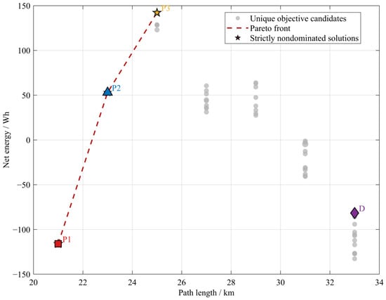
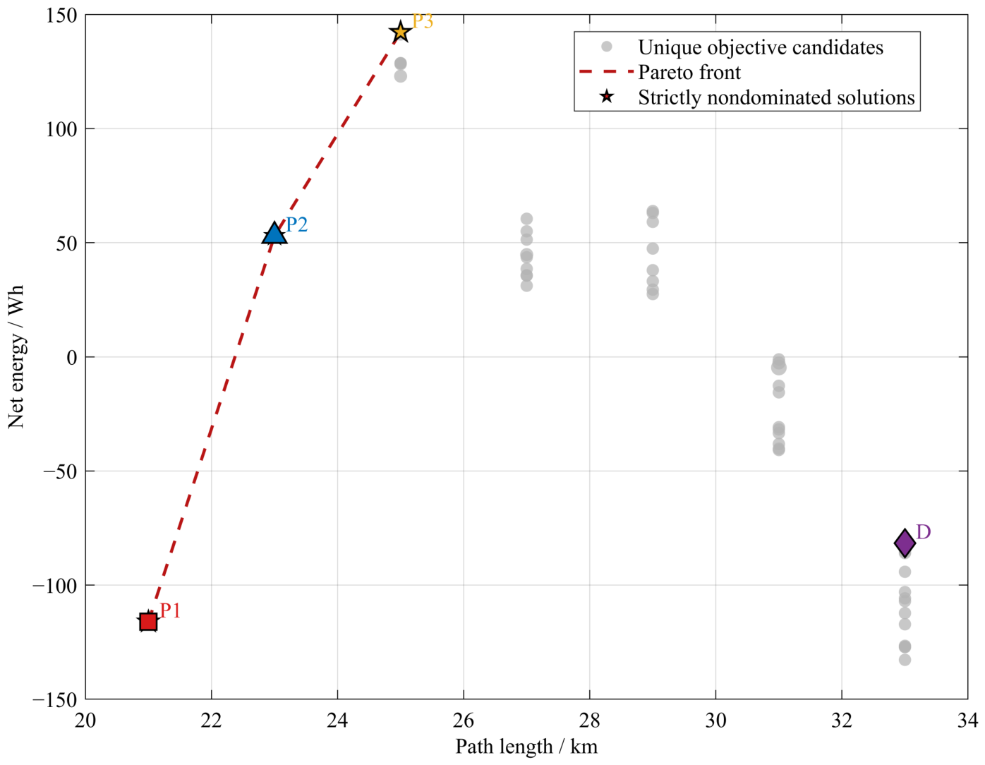
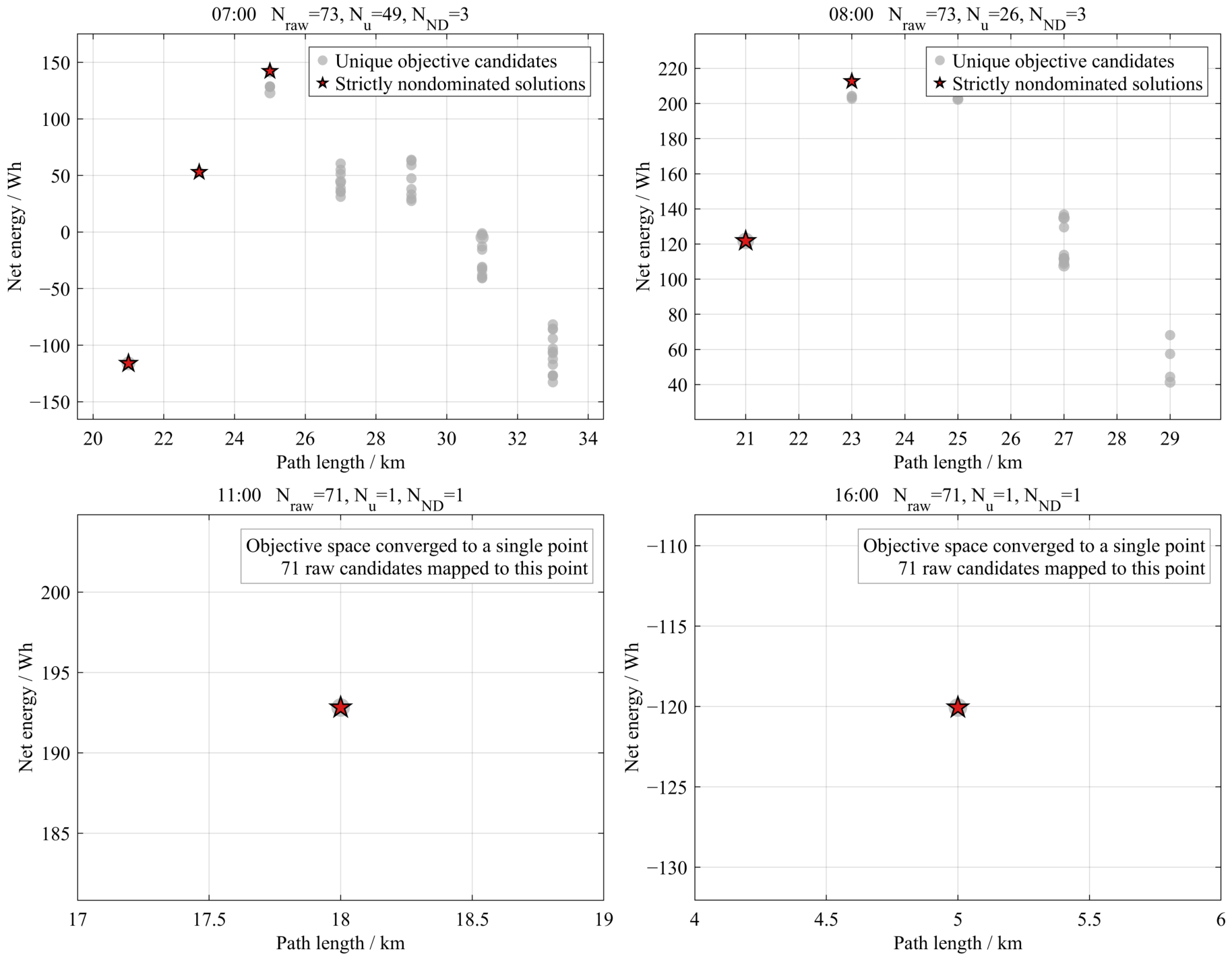
To analyse the trade-off capability of ME-DMOEA regarding net energy and range objectives, candidate solutions at the 08:00 rolling moment were selected for analysis. At this moment, a total of 73 feasible candidate solutions were obtained, which were reduced to 26 unique objective points after removing duplicates based on objective values, among which 3 were strictly non-dominated solutions, as shown in Figure 6. The dashed lines in the figure are only used to connect discrete non-dominated solutions to aid in identifying the Pareto front and do not indicate the existence of continuous feasible solutions between adjacent solutions.

Figure 6. 0800 Candidate target space and Pareto frontier.

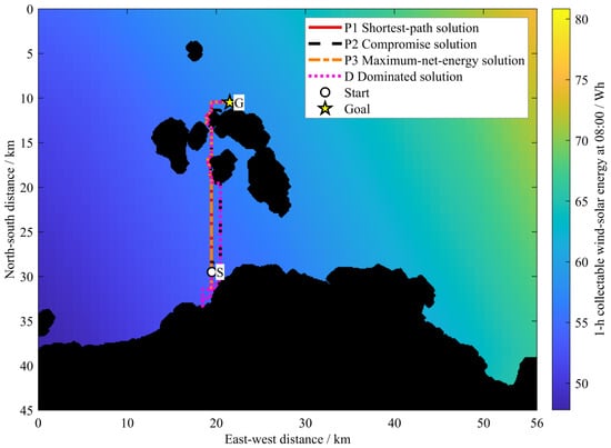
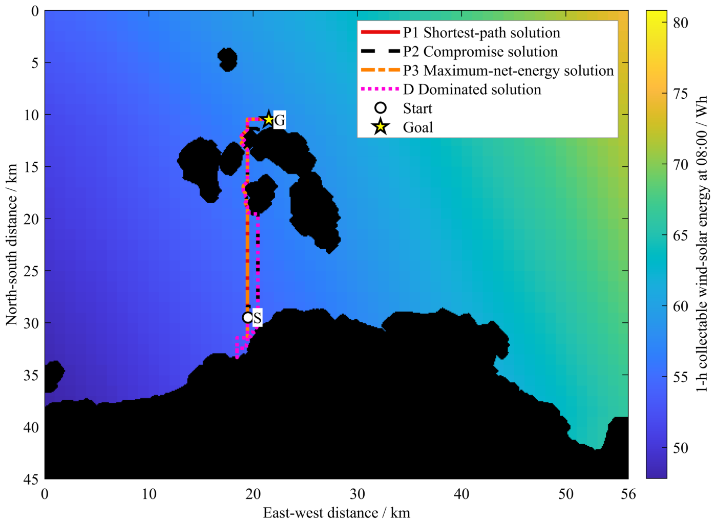
The three representative non-dominated solutions P1, P2 and P3 have ranges of 21 km, 23 km and 25 km, with corresponding net energies of −116.08 Wh, 51.87 Wh and 142.22 Wh, respectively. The results indicate that a longer range allows the unmanned vessel to pass through areas with more favourable energy conditions and increase energy collection, but at the same time increases propulsion energy consumption, thus creating a clear Pareto trade-off between the two objectives. Figure 7 further presents the three Pareto paths and a representative dominated path D, showing that merely increasing the range does not guarantee a higher net energy gain. Different detours in Figure 7 encounter different energy conditions and incur propulsion costs; the dominated path D illustrates that additional harvesting may not offset the extra propulsion consumption.

Figure 7. 0800 Representative Pareto paths and dominated paths.

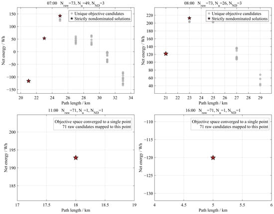
Figure 8 shows the candidate objective spaces at 07:00, 08:00, 11:00, and 16:00. The numbers of unique objective points are 49, 26, 1, and 1, respectively, with 3, 3, 1, and 1 non-dominated solutions. The contraction is consistent with reduced route flexibility as the mission progresses; it does not, by itself, demonstrate superior optimizer convergence.

Figure 8. Evolution of candidate objective space at four rolling instants: 07:00, 08:00, 11:00, and 16:00.

5.4. Comparison of Baseline Algorithms and Results Analysis

The A* algorithm is used as a benchmark method for shortest path guidance [33]. The second benchmark is an energy-greedy strategy, which prioritises navigable areas with higher available energy at each decision-making stage [34], without explicitly considering the propulsion energy expenditure incurred by detours. The three methods use the same starting point, rendezvous point, dynamic energy field, obstacle map and energy consumption parameters.

Although A* and ME-DMOEA share the same movement constraints at each grid resolution, their route-selection criteria differ. The implemented A* minimises the number of four-neighbor steps on the 1 km grid, using unit step costs and a Manhattan-distance heuristic. In contrast, ME-DMOEA jointly considers net energy and executable voyage distance, while also optimising the hourly movement and dwelling schedule. Both methods are subject to the same fine-grid obstacle constraints and maximum sailing speed. Consequently, a shortest path in the coarse-grid step-count sense is not necessarily the shortest executable path after 100 m obstacle repair. The reported differences should therefore be interpreted under the specified A* baseline and common fine-grid evaluation procedure, rather than as improvements arising from more permissive movement directions for ME-DMOEA.

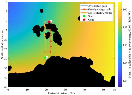
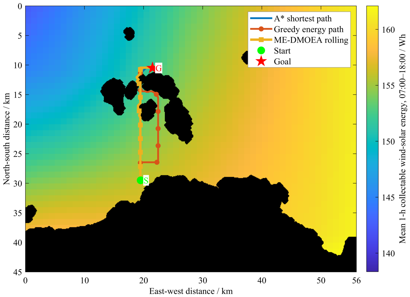
Under the above conditions, MATLAB simulation was carried out, and the trajectories obtained by the three algorithms are shown in Figure 9, with their range and energy balance results presented in Table 3.

Figure 9. Route planning using three algorithmic approaches.

Table 3 summarizes the fine-grid path repair results and the performance of the three methods under the two mission scenarios. In S1, fine-grid BFS repair eliminated all four obstacle intersections in the original ME-DMOEA path. The final executable path length was 22.16 km, with a net energy of 400.47 Wh, compared with 364.64 Wh for the four-neighbor A* baseline and 163.46 Wh for Greedy. In S2, ME-DMOEA achieved a net energy of 446.89 Wh over 19.94 km, compared with 364.07 Wh over 21.66 km for A* and 164.16 Wh over 26.47 km for Greedy.

Compared with A*, ME-DMOEA increased net energy by 35.83 Wh (9.83%) in S1 despite having the same voyage distance and propulsion consumption; thus, the improvement resulted from greater renewable-energy harvesting. In S2, the net-energy improvement of 82.82 Wh (22.75%) was attributable to 5.10 Wh of additional harvested energy and 77.72 Wh of reduced propulsion consumption, with a 1.72 km shorter voyage. This distance reduction reflects differences in route selection and the resulting fine-grid executable geometry; it does not result from permitting diagonal movements for ME-DMOEA on the coarse planning grid. The energy-oriented detour of Greedy in Figure 9 further illustrates this trade-off: in S2, Greedy harvested 11.44 Wh more than ME-DMOEA but consumed 294.18 Wh more propulsion energy. Relative to the reference usable-capacity value of 8192 Wh, the net-energy improvements over A* correspond to approximately 0.44% and 1.01% in S1 and S2, respectively, representing potential energy surplus rather than experimentally verified endurance gains or actual transferred energy.

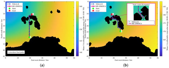
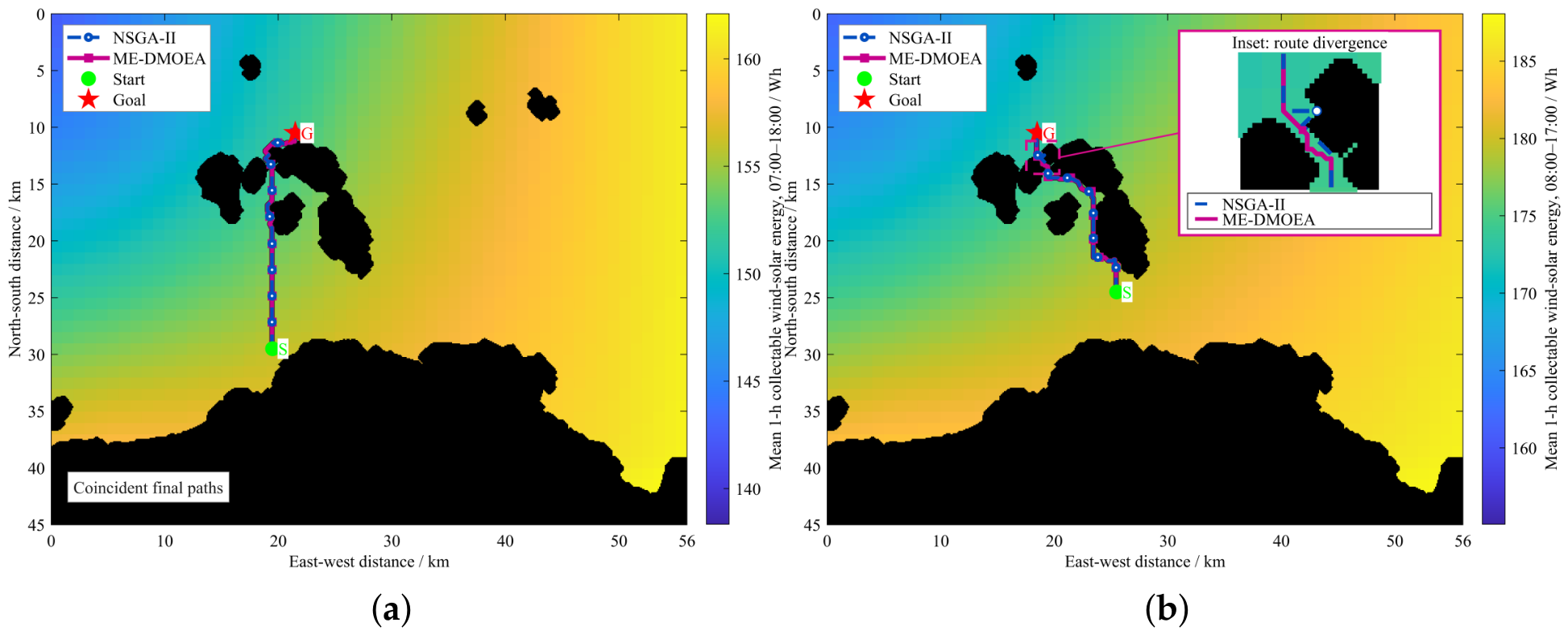
Table 4 reports 30 paired runs per configuration using the tested ERA5 inputs. The optimizers tied in S1; in S2, ME-DMOEA’s mean net-energy advantages were 22.88 Wh on 15 August 2025 and 13.21 Wh on 30 June 2025 (Wilcoxon p = 0.000137 and 0.00314, respectively), supporting a scenario-dependent advantage rather than universal superiority. For S1, the ME-DMOEA values are 400.47 Wh and 22.16 km in Table 3, compared with 401.47 Wh and 22.13 km in Table 4. This small discrepancy reflects the different execution protocols and should not be interpreted as an additional algorithmic improvement. Figure 10 shows representative paired runs: coincident S1 paths (seed 1) and local S2 route divergence near obstacles (seed 4, inset). Statistical conclusions rely on all 30 pairs, not these examples alone. However, these comparative gains should not be interpreted as evidence of a statistically demonstrated benefit from rolling replanning itself, because the Rolling ON/OFF ablation in Section 5.5 did not show a significant net-energy difference.

Table 4. Statistical comparison of ME-DMOEA and NSGA-II over 30 independent paired runs.

Scenario/Date	ME-DMOEA Net (Wh)	NSGA-II Net (Wh)	ME-DMOEA Path (km)	NSGA-II Path (km)	Mean $\mathbf{\Delta }$Net (Wh)	W/T/L	p
S1/15 August 2025	$401.47\pm 0.00$	$401.47\pm 0.00$	$22.13\pm 0.00$	$22.13\pm 0.00$	0.00	0/30/0	1.000
S2/15 August 2025	$446.28\pm 2.16$	$423.40\pm 22.96$	$19.96\pm 0.07$	$20.45\pm 0.51$	+22.88	19/7/4	0.000137
S2/30 June 2025	$977.20\pm 17.13$	$963.99\pm 21.64$	$20.23\pm 0.37$	$20.49\pm 0.46$	+13.21	25/0/5	0.00314

Notes: Values are mean ± standard deviation over 30 paired runs. $\Delta$Net denotes the mean net-energy difference (ME-DMOEA minus NSGA-II). W/T/L represents wins/ties/losses. The p-values are from two-sided Wilcoxon signed-rank tests (S1: all ties, $p=1$).

Figure 10. Representative final executable paths obtained by ME-DMOEA and NSGA-II in (a) Scenario S1 and (b) Scenario S2.

With the final feasible Table 3 routes, harvested energy, and mission durations fixed, varying the 45 Wh/km propulsion coefficient by $\pm 20\%$ left ME-DMOEA’s net-energy advantage over four-neighbor A* positive: 35.83 Wh in S1 and 67.28–98.36 Wh in S2. Common hotel-load power changes of $\pm 20\%$ left relative differences unchanged because mission durations were equal within each scenario. This fixed-route analysis does not replace realistic propulsion modeling of speed variations, ocean currents, or sea-state effects.

5.5. Rolling-Horizon Ablation Study

To assess the contribution of rolling-horizon replanning, an ablation study was conducted under Scenario S2 using the ERA5 energy field of 15 August 2025. Rolling ON re-optimized the remaining route at successive planning stages, whereas Rolling OFF optimized the complete route once and subsequently executed the initial plan without replanning. Both configurations used the same environmental inputs, constraints, and optimization settings, with 30 paired random seeds.

As shown in Table 5, Rolling ON achieved a slightly higher mean net energy, with 4 wins, 23 ties, and 3 losses. The mean paired improvement was approximately 0.68 Wh, but the difference was not statistically significant (two-sided exact Wilcoxon test, $p=0.203$). Across the 30 paired runs, the recorded rolling-computation and audit times were $58.72\pm 3.90$ s for Rolling ON and $8.49\pm 0.20$ s for Rolling OFF. This timing metric includes computation and verification overhead and therefore does not represent isolated optimizer execution time. Rolling replanning also required substantially more objective evaluations. Therefore, the present ablation study does not provide statistical evidence that rolling replanning itself improves net energy when the complete environmental sequence is known in advance. In this study, the rolling mechanism should therefore be regarded primarily as an adaptive route-updating mechanism rather than as a statistically demonstrated source of additional net-energy gain.

Table 5. Ablation results of the rolling-horizon mechanism under Scenario S2 (30 paired runs).

Configuration	Net Energy (Wh)	Path Length (km)	Feasibility (%)	Evaluations
Rolling ON	$446.28\pm 2.16$	19.959	100	36,386
Rolling OFF	$445.59\pm 3.15$	19.973	100	5049

Note: Net energy is reported as mean ± standard deviation. Path length and evaluations are mean values.

5.6. Limitations of the Current Study

The results of this study should be interpreted in light of the model assumptions adopted. First, the propulsion energy consumption is simplified as a linear function of the voyage distance, without explicitly considering speed variations, ocean currents, and the added resistance of waves; therefore, the present results mainly reflect the coupling relationship between path geometry and the time-varying energy distribution. Second, this paper assumes that the rendezvous position of the energy-receiving vessel is known and does not model the inter-vessel energy transfer efficiency or the actual berthing process; consequently, $E_{\mathrm{net}}$ represents the energy surplus potentially available for external resupply rather than the actually transferred energy. Third, this paper constructs the time-varying energy field using hourly environmental data and evaluates the planning method through numerical simulation, without closed-loop verification based on real-vessel online observations. These simplifications facilitate the isolated analysis of the role of net-energy-aware path planning, but they also limit the direct generalization of the results to actual offshore operating conditions.

Furthermore, the present obstacle model considers static islands, reefs, and coastlines, but does not simulate moving vessels, dynamic collision risks, or COLREGs-compliant avoidance maneuvers. Collision-case-based testing scenarios derived from actual maritime accidents provide a relevant direction for future validation of the framework under realistic vessel encounters [35]. In addition, the rolling-horizon ablation uses known hourly ERA5 energy sequences and does not establish its benefit under forecast uncertainty or unexpected environmental disturbances. Future application therefore requires integration with traffic-aware collision avoidance and validation through more realistic scenarios and real-vessel trials.

6. Conclusions

This study integrates time-varying wind–solar energy fields, onboard energy balance, and Pareto optimization into a receding-horizon ME-DMOEA for nearshore mobile energy resupply. A 1 km grid supports energy evaluation and route search, while a 100 m grid supports obstacle checking and local repair. In the evaluated scenarios, the final executable-path results showed that ME-DMOEA achieved net energies of 400.47 Wh in S1 and 446.89 Wh in S2, exceeding the implemented four-neighbor A* baseline by 35.83 Wh and 82.82 Wh, respectively. Repeated comparisons with NSGA-II showed identical results in S1 and higher mean net energy for ME-DMOEA in S2 under both tested ERA5 energy fields, while the rolling-horizon ablation revealed no statistically significant additional net-energy gain under the fully known environmental sequence. The results indicate that incorporating renewable energy harvesting together with the energy consumption of the unmanned surface vehicle into path evaluation helps achieve a more reasonable energy–range trade-off. Future work will address moving rendezvous points, propulsion models accounting for currents and sea states, COLREGs-compliant avoidance in dynamic traffic, and inter-vessel transfer efficiency, with collision-case-based testing and real-vessel validation.

References

- Wang, G.; Xu, T.; Yang, M.; Niu, W. Review on renewable energy systems of unmanned marine vehicles and guidance for energy selection. Renew. Sustain. Energy Rev. 2025, 224, 116085. [Google Scholar] [CrossRef] [Scilit]
- Liang, X.; Wang, P.; Zhang, X.; Wen, B.; Li, X.; Tian, X. Multi-objective robust energy management for environment powered unmanned surface vehicles. Ocean Eng. 2022, 247, 110624. [Google Scholar] [CrossRef] [Scilit]
- Fernandes, J.F.P.; Assunção, M.; Serrano, D.; Afonso, P.; Pinheiro, P.; Marques, H.; Neves, J.; Teodoro, P.; Póvoa, R.; Marat-Mendes, R.; et al. A smart energy management system for surface unmanned vehicles for border surveillance missions. Sci. Rep. 2025, 15, 23684. [Google Scholar] [CrossRef] [Scilit] [PubMed]
- Chu, Y.; Gao, Q.; Yue, Y.; Lim, E.G.; Paoletti, P.; Ma, J.; Zhu, X. Evolution of unmanned surface vehicle path planning: A comprehensive review of basic, responsive, and advanced strategic pathfinders. Drones 2024, 8, 540. [Google Scholar] [CrossRef] [Scilit]
- Liao, Y.; Li, K.; Zhao, Y.; Tang, H.; Zhang, M.; Liu, X.; Yuan, Z.M. Energy optimal path planning of ocean-energy driven unmanned surface vehicles. Ocean Eng. 2025, 327, 120965. [Google Scholar] [CrossRef] [Scilit]
- Minak, G. Solar Energy-Powered Boats: State of the Art and Perspectives. J. Mar. Sci. Eng. 2023, 11, 1519. [Google Scholar] [CrossRef] [Scilit]
- Yuan, J.; Liu, H.; Zhang, W. Waypoint tracking control for autonomous mobile sampling and dissolved oxygen enrichment of unmanned surface vehicle. J. Robot. 2022, 2022, 3652329. [Google Scholar] [CrossRef] [Scilit]
- Marini, S.; Gjeci, N.; Govindaraj, S.; But, A.; Sportich, B.; Ottaviani, E.; García Márquez, F.P.; Bernalte Sanchez, P.J.; Pedersen, J.; Clausen, C.V.; et al. ENDURUNS: An Integrated and Flexible Approach for Seabed Survey Through Autonomous Mobile Vehicles. J. Mar. Sci. Eng. 2020, 8, 633. [Google Scholar] [CrossRef] [Scilit]
- Davis, A.; Wills, P.S.; Garvey, J.E.; Fairman, W.; Karim, M.A.; Ouyang, B. Developing and field testing path planning for robotic aquaculture water quality monitoring. Appl. Sci. 2023, 13, 2805. [Google Scholar] [CrossRef] [Scilit]
- Jia, Q.; Liao, Y.; Xu, P.; Wang, Z.; Pang, S.; Li, X. Long-Endurance Dynamic Path Planning Method of NSV Considering Wind Energy Capture. J. Mar. Sci. Eng. 2021, 9, 878. [Google Scholar] [CrossRef] [Scilit]
- Xing, B.; Yu, M.; Liu, Z.; Tan, Y.; Sun, Y.; Li, B. A review of path planning for unmanned surface vehicles. J. Mar. Sci. Eng. 2023, 11, 1556. [Google Scholar] [CrossRef] [Scilit]
- Niu, H.; Lu, Y.; Savvaris, A.; Tsourdos, A. Efficient path planning algorithms for unmanned surface vehicle. IFAC-PapersOnLine 2016, 49, 121–126. [Google Scholar] [CrossRef] [Scilit]
- Niu, H.; Lu, Y.; Savvaris, A.; Tsourdos, A. An energy-efficient path planning algorithm for unmanned surface vehicles. Ocean Eng. 2018, 161, 308–321. [Google Scholar] [CrossRef] [Scilit]
- Niu, H.; Ji, Z.; Savvaris, A.; Tsourdos, A. Energy efficient path planning for unmanned surface vehicle in spatially-temporally variant environment. Ocean Eng. 2020, 196, 106766. [Google Scholar] [CrossRef] [Scilit]
- Gu, S.; Zhou, C.; Wen, Y.; Xiao, C.; Knoll, A. Motion planning for an unmanned surface vehicle with wind and current effects. J. Mar. Sci. Eng. 2022, 10, 420. [Google Scholar] [CrossRef] [Scilit]
- Yuan, X.; Tong, C.; He, G.; Wang, H. Unmanned Vessel Collision Avoidance Algorithm by Dynamic Window Approach Based on COLREGs Considering the Effects of the Wind and Wave. J. Mar. Sci. Eng. 2023, 11, 1831. [Google Scholar] [CrossRef] [Scilit]
- Luo, J.; Zhuang, J.; Jin, M.; Xu, F.; Su, Y. An energy-efficient path planning method for unmanned surface vehicle in a time-variant maritime environment. Ocean Eng. 2024, 301, 117544. [Google Scholar] [CrossRef] [Scilit]
- Namgung, H.; Kim, J.S.; Jang, D.U. Path planning and collision avoidance technologies for maritime autonomous surface ships: A review of COLREGs compliance, algorithmic trends and the navigation-GPT framework. J. Navig. 2025, 78, 430–450. [Google Scholar] [CrossRef] [Scilit]
- Namgung, H. Local Route Planning for Collision Avoidance of Maritime Autonomous Surface Ships in Compliance with COLREGs Rules. Sustainability 2022, 14, 198. [Google Scholar] [CrossRef] [Scilit]
- MahmoudZadeh, S.; Abbasi, A.; Yazdani, A.; Wang, H.; Liu, Y. Uninterrupted path planning system for multi-USV sampling mission in a cluttered ocean environment. Ocean Eng. 2022, 254, 111328. [Google Scholar] [CrossRef] [Scilit]
- Zhang, Y.; Shi, G.; Liu, J. Dynamic energy-efficient path planning of unmanned surface vehicle under time-varying current and wind. J. Mar. Sci. Eng. 2022, 10, 759. [Google Scholar] [CrossRef] [Scilit]
- Chowdhury, R.; Navsalkar, A.; Subramani, D. GPU-Accelerated Multi-Objective Optimal Planning in Stochastic Dynamic Environments. J. Mar. Sci. Eng. 2022, 10, 533. [Google Scholar] [CrossRef] [Scilit]
- Sudha, S.K.R.; Mishra, D.; Hameed, I.A. A coverage path planning approach for environmental monitoring using an unmanned surface vehicle. Ocean Eng. 2024, 310, 118645. [Google Scholar] [CrossRef] [Scilit]
- Farina, M.; Deb, K.; Amato, P. Dynamic multiobjective optimization problems: Test cases, approximations, and applications. IEEE Trans. Evol. Comput. 2004, 8, 425–442. [Google Scholar] [CrossRef] [Scilit]
- Jiang, S.; Zou, J.; Yang, S.; Yao, X. Evolutionary dynamic multi-objective optimisation: A survey. ACM Comput. Surv. 2022, 55, 76. [Google Scholar] [CrossRef] [Scilit]
- Wu, Y.; Shi, L.; Liu, X. A new dynamic strategy for dynamic multi-objective optimization. Inf. Sci. 2020, 529, 116–131. [Google Scholar] [CrossRef] [Scilit]
- Zheng, J.; Zhou, Y.; Zou, J.; Yang, S.; Ou, J.; Hu, Y. A prediction strategy based on decision variable analysis for dynamic multi-objective optimization. Swarm Evol. Comput. 2021, 60, 100786. [Google Scholar] [CrossRef] [Scilit]
- Chen, L.; Wang, H.; Pan, D.; Wang, H.; Gan, W.; Wang, D.; Zhu, T. Dynamic multiobjective evolutionary algorithm with adaptive response mechanism selection strategy. Knowl.-Based Syst. 2022, 246, 108691. [Google Scholar] [CrossRef] [Scilit]
- Wang, P.; Ma, Y.; Wang, M. A dynamic multi-objective optimization evolutionary algorithm based on particle swarm prediction strategy and prediction adjustment strategy. Swarm Evol. Comput. 2022, 75, 101164. [Google Scholar] [CrossRef] [Scilit]
- Wu, F.; Chen, J.; Wang, W. A dynamic multi-objective evolutionary algorithm based on prediction. J. Comput. Des. Eng. 2023, 10, 1–15. [Google Scholar] [CrossRef] [Scilit]
- Peng, H.; Mei, C.; Zhang, S.; Luo, Z.; Zhang, Q.; Wu, Z. Multi-strategy dynamic multi-objective evolutionary algorithm with hybrid environmental change responses. Swarm Evol. Comput. 2023, 82, 101356. [Google Scholar] [CrossRef] [Scilit]
- Gong, D.; Rong, M.; Hu, N.; Wang, Y.; Pedrycz, W.; Yang, S. A prediction and weak coevolution-based dynamic constrained multiobjective optimization. IEEE Trans. Evol. Comput. 2025, 29, 1328–1342. [Google Scholar] [CrossRef] [Scilit]
- Zhang, H.; Tao, Y.; Zhu, W. Global Path Planning of Unmanned Surface Vehicle Based on Improved A-Star Algorithm. Sensors 2023, 23, 6647. [Google Scholar] [CrossRef] [Scilit] [PubMed]
- Aslan, S. Back-and-Forth (BaF): A New Greedy Algorithm for Geometric Path Planning of Unmanned Aerial Vehicles. Computing 2024, 106, 2811–2849. [Google Scholar] [CrossRef] [Scilit]
- Lee, J.Y.; Namgung, H.; Kim, J.S. Development of collision-case-based testing scenarios for validating autonomous ship collision-avoidance algorithms. Brodogradnja 2026, 77, 77204. [Google Scholar] [CrossRef] [Scilit]
Disclaimer/Publisher’s Note: The statements, opinions and data contained in all publications are solely those of the individual author(s) and contributor(s) and not of MDPI and/or the editor(s). MDPI and/or the editor(s) disclaim responsibility for any injury to people or property resulting from any ideas, methods, instructions or products referred to in the content. |
© 2026 by the authors. Licensee MDPI, Basel, Switzerland. This article is an open access article distributed under the terms and conditions of the Creative Commons Attribution (CC BY) license.