Path Planning and Trajectory Tracking of an Underwater Quadrotor Vehicle Using Enhanced RRT and Disturbance-Observer-Assisted MPC–PID

Abstract

Underwater quadrotor vehicles operating in complex nearshore environments face challenges in three-dimensional path planning, obstacle-triggered replanning, and trajectory tracking under external disturbances. To address these issues, this paper evaluates an enhanced rapidly exploring random tree (iRRT) planner and a model predictive control–proportional–integral–derivative (MPC–PID) tracking strategy with residual disturbance estimation. The planner combines guided sampling, environment-aware adaptive extension, collision-checked reverse greedy pruning, and cubic B-spline smoothing. A bisection-based handoff reconnects the remaining safe path after a newly introduced obstacle; post-solution informed sampling is examined separately as an ablation. The tracking controller is evaluated on a nonlinear six-degree-of-freedom vehicle model under a seeded, wave-shaped disturbance proxy. In 30 runs on the original voxel map, both RRT and iRRT produced safe paths in the static and fixed-obstacle replanning cases under the same additional radius-two voxel-neighborhood test. Relative to RRT, iRRT reduced the mean number of raw path nodes by 37.4% in the static case and 12.8% after replanning, whereas its small mean path-length differences were not conclusive. Under matched paths and disturbance phases, adding residual estimation to MPC–PID reduced mean position RMSE by 12.1% on the static path and 9.7% on the replanned path. Component ablations and additional synthetic maps further examine the contributions and limits of the planning modules. These results support the proposed integration under the stated numerical assumptions; measured hydrodynamics and vehicle experiments remain to be investigated.

1. Introduction

Underwater robotic vehicles are increasingly used in marine observation, seabed mapping, underwater infrastructure inspection, shallow-water aquaculture, and search-and-rescue missions [1,2,3]. Compared with diver-based and towed-platform operations, these vehicles can operate for extended periods under low visibility, high hydrostatic pressure, complex terrain, and strong environmental disturbances, making them particularly valuable for nearshore applications [4,5]. Nearshore environments, however, are often characterized by irregular seabed topography, dense reefs, newly encountered obstacles, and wave-induced disturbances. Under such conditions, an underwater vehicle must rapidly generate a safe and collision-free path in three-dimensional space while ensuring that the resulting path is sufficiently smooth and trackable [6,7]. Path planning and trajectory-tracking control therefore cannot be treated as completely independent modules, because redundant waypoints, abrupt directional changes, and discontinuities in a planned path can increase the burden on the downstream controller and degrade tracking performance [8]. This study addresses these coupled planning and control challenges for an underwater quadrotor vehicle operating in a complex nearshore environment.

Existing underwater path-planning methods can be broadly classified into graph-search methods, swarm-intelligence and evolutionary algorithms, learning-based methods, and sampling-based planners. Among graph-search methods, A* is widely used because of its well-defined search procedure, reproducible performance, and straightforward implementation [9]. Lai et al. [10] combined an enhanced A* algorithm with the dynamic window approach and improved search efficiency and path smoothness by modifying the search direction, evaluation function, and local obstacle-avoidance mechanism. However, the computational and memory requirements of graph-search methods increase considerably with grid resolution and workspace dimensionality, particularly in three-dimensional environments. Ant colony optimization (ACO) is a representative swarm-intelligence algorithm with strong global-search capability. Meng et al. [11] introduced an improved heuristic function and pheromone-update strategy into ACO, while Yuan et al. [12] combined ACO with a three-dimensional dynamic window approach to improve path-planning performance in complex environments. Nevertheless, the convergence rate and solution quality of such methods can be sensitive to parameter settings and stochastic initialization. Differential evolution and reinforcement learning have also been applied to path-planning problems subject to multiple constraints, with fitness-function design, cooperative evolution, and weighted guidance used to improve global exploration and energy-related performance [13,14,15].

Sampling-based planners, particularly the rapidly exploring random tree (RRT) algorithm and its variants, are well suited to continuous and high-dimensional configuration spaces. Conventional RRT can rapidly obtain a feasible path without discretizing the entire workspace in advance [16]. RRT-Connect improves single-query efficiency through bidirectional tree expansion [17], whereas RRT* achieves asymptotic optimality through a rewiring mechanism [18]. Informed RRT* further restricts sampling to a heuristic subset after an initial solution has been obtained, thereby accelerating convergence toward a lower-cost path [19]. These characteristics have motivated the application of RRT-based methods to three-dimensional underwater path planning. For example, Song et al. [20] developed a reinforcement-learning-assisted bidirectional RRT method to improve sampling efficiency, while Ge et al. [21] incorporated RRT* into a cost-valley framework for long-horizon adaptive sampling by autonomous underwater vehicles. Despite these advances, conventional RRT remains affected by inefficient unguided sampling, poor adaptability of a fixed extension step, numerous redundant waypoints, and abrupt directional changes. Moreover, when a previously unknown obstacle invalidates the original path during execution, an inappropriate replanning start point may produce a discontinuous or unnecessarily circuitous transition between the original and replanned path, thereby increasing the difficulty of subsequent trajectory tracking.

Trajectory-tracking methods for underwater vehicles include proportional–integral–derivative (PID) control, backstepping control, sliding-mode control, adaptive control, and model predictive control (MPC). PID control is structurally simple, computationally inexpensive, and straightforward to implement. However, its performance depends strongly on parameter tuning, and overshoot or oscillation may occur in systems with strong nonlinearities, multivariable coupling, and external disturbances [22]. Backstepping and sliding-mode control are well suited to nonlinear system dynamics. Adaptive backstepping, terminal sliding-mode control, and high-order sliding-mode control have therefore been employed to improve the tracking accuracy of autonomous underwater vehicles under model uncertainty and environmental disturbances [23,24,25,26]. Nevertheless, their practical implementation may still be affected by chattering, abrupt control action, or dependence on accurate model information and uncertainty bounds.

MPC formulates trajectory tracking as a receding-horizon optimization problem and can explicitly account for state constraints, input constraints, and multivariable coupling. It has therefore been widely investigated for underwater-vehicle trajectory tracking and obstacle-avoidance control [27,28,29]. Nevertheless, prediction accuracy and closed-loop performance can deteriorate in the presence of model mismatch, unmodeled dynamics, and environmental disturbances. In addition, the computational burden of online optimization may restrict the prediction horizon or control-update rate [30,31]. Disturbance observers, extended-state observers, and sliding-mode observers have consequently been introduced to estimate ocean-current disturbances, wave-induced disturbances, and model uncertainties online [32,33,34]. The estimated disturbances can then be incorporated into the control law as compensation terms to improve tracking accuracy and disturbance rejection [35,36].

Although sampling-based planners and predictive controllers have been studied extensively, their performance is often evaluated separately. In underwater navigation, a path regenerated after obstacle detection must remain collision-free and trackable under disturbances. This study therefore evaluates a reproducible planning–replanning–tracking pipeline, with separate tests for path postprocessing, replanning handoff, and disturbance estimation.

The main contributions of this study are summarized as follows.

(1)

We implement an RRT-based planning pipeline with guided sampling, local step adaptation, collision-checked reverse greedy pruning, and B-spline smoothing with a safe-path fallback. Thirty-run comparisons use a common collision test and postprocessing rule for ACO, A*, RRT, and the corresponding iRRT configuration; a separate equal-budget ablation evaluates post-solution informed sampling and the other planner components. In the tested matched-budget sequence, collision-checked reverse greedy pruning produced the largest reduction in mean safe-path length, whereas optional post-solution informed sampling showed no consistent independent gain.

(2)

We evaluate replanning after a newly introduced obstacle using a path-domain bisection rollback and a guarded connection policy. The retained prefix and regenerated path are checked under the updated map. We also examine a separate, controlled continuously moving-obstacle case with predicted obstacle motion and six-degree-of-freedom trajectory replay.

(3)

We combine a translational MPC outer loop, continuously weighted PID correction, and residual-based disturbance estimation with a nonlinear six-degree-of-freedom plant, attitude PD control, and four-thruster allocation. Matched-path and matched-wave comparisons quantify the contribution of disturbance estimation, while the planner ablation and safety checks establish the scope of the observed improvements.

2. System Modeling and Problem Formulation

2.1. Kinematic and Dynamic Models

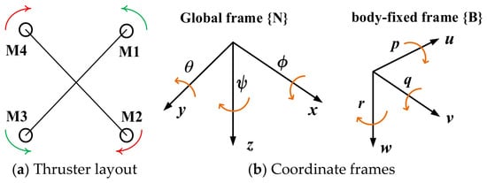
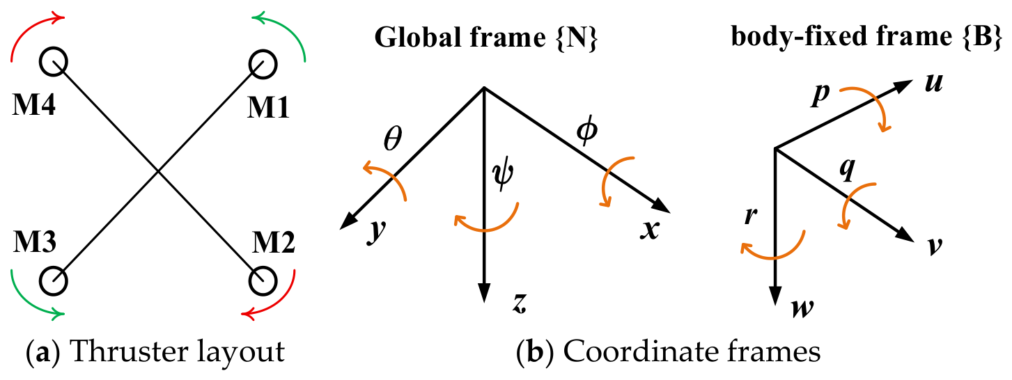
The simulated underwater vehicle is represented as a six-degree-of-freedom rigid body driven by four nonnegative thruster forces. Figure 1 illustrates the inertial and body-fixed coordinate frames and a schematic four-thruster layout. The equivalent force and moment allocation used in the numerical model is specified separately in Equation (12).

Figure 1. Schematic four-thruster arrangement and coordinate frames of the underwater vehicle: (a) thruster layout and (b) inertial frame {N} and body-fixed frame {B}. The equivalent force-and-moment allocation used in the simulation is given in Equation (12).

The vehicle kinematics relate the translational and rotational velocities expressed in the body-fixed frame to the time derivatives of the position and attitude expressed in the inertial frame [37]:

$${\left[\dot{x},\dot{y},\dot{z},\dot{\varphi },\dot{\theta },\dot{\psi }\right]}^{\mathrm{T}}=\left[\begin{array}{cc}{\mathit{R}}_1& {\mathbf{0}}_{3\times 3}\\ {\mathbf{0}}_{3\times 3}& {\mathit{R}}_2\end{array}\right]\left[\begin{array}{c}{\mathit{v}}_{\mathrm{b}}\\ {\mathit{\omega }}_{\mathrm{b}}\end{array}\right]$$

(1)

where η₁ = [x,y,z]^T and η₂ = [ϕ,θ,ψ]^T denote the position and attitude vectors in the inertial frame, respectively; v_b = [u,v,w]^T and ω_b = [p,q,r]^T denote the linear- and angular-velocity vectors in the body-fixed frame. The six degrees of freedom correspond to surge, sway, heave, roll, pitch, and yaw. The transformation matrices R₁ and R₂, which map the body-fixed linear and angular velocities to the inertial frame, are given by Equations (2) and (3).

$$\begin{array}{c}{\mathit{R}}_1=\left[\begin{array}{ccc}\cos \psi & -\sin \psi & 0\\ \sin \psi & \cos \psi & 0\\ 0& 0& 1\end{array}\right]\cdot \left[\begin{array}{ccc}\cos \theta & 0& \sin \theta \\ 0& 1& 0\\ -\sin \theta & 0& \cos \theta \end{array}\right]\cdot \left[\begin{array}{ccc}1& 0& 0\\ 0& \cos \varphi & -\sin \varphi \\ 0& \sin \varphi & \cos \varphi \end{array}\right]\\ =\left[\begin{array}{ccc}\cos \psi \cos \varphi & -\sin \psi \cos \varphi +\sin \varphi \sin \theta \cos \psi & \sin \psi \sin \varphi +\cos \varphi \sin \theta \cos \psi \\ \sin \psi \cos \theta & \cos \psi \cos \varphi +\sin \varphi \sin \theta \sin \psi & -\cos \psi \sin \varphi +\cos \varphi \sin \theta \sin \psi \\ -\sin \theta & \cos \theta \sin \varphi & \cos \theta \cos \varphi \end{array}\right]\end{array}$$

(2)

$${\mathit{R}}_2=\left[\begin{array}{ccc}1& \tan \theta \sin \varphi & \tan \theta \cos \varphi \\ 0& \cos \varphi & -\sin \varphi \\ 0& \sin \varphi /\cos \theta & \cos \varphi /\cos \theta \end{array}\right]$$

(3)

The following assumptions are adopted in establishing the dynamic model:

(1)

The vehicle is treated as a rigid body moving in three-dimensional space. Elastic deformation is neglected, and the relative positions of its components remain fixed.

(2)

Seawater is modeled as a homogeneous, incompressible fluid with constant density.

(3)

The four thrusters are represented by the equivalent force-and-moment allocation in Equation (12). Roll and pitch restoring moments are represented by the simplified terms in Equation (11); separate center-of-gravity and center-of-buoyancy locations are not specified. The commanded tilt is limited to 30°, while the actual attitude is evaluated separately in the simulations. Following the standard six-degree-of-freedom marine-vehicle formulation [38], the vehicle dynamics are written as

$$\mathit{M}\dot{\mathit{v}}+\mathit{C}\left(\mathit{v}\right)\mathit{v}+\mathit{D}\left(\mathit{v}\right)\mathit{v}+\mathit{g}\left(\mathit{\eta }\right)=\mathit{\tau }+{\mathit{\tau }}_d$$

(4)

where $\mathit{v}={\left({\mathit{v}}_{\mathrm{b}},{\mathit{\omega }}_{\mathrm{b}}\right)}^{\mathrm{T}}$ is the body-fixed velocity vector; M is the inertia matrix; C(v) is the Coriolis and centripetal matrix; D(v) is the hydrodynamic damping matrix; g(η) is the restoring-force-and-moment vector; τ is the control-input vector; and τ_d is the external-disturbance vector.

Equation (4) is the general six-degree-of-freedom model. The numerical experiments use a 12-state nonlinear implementation with diagonal effective inertia, componentwise damping, and simplified restoring moments. The outer-loop MPC uses the separate translational prediction model described in Section 3.2. All vehicle coefficients and integration settings are reported in Supplementary Table S2; they are simulation parameters rather than values identified from a physical vehicle.

The inertia matrix is composed of the rigid-body inertia matrix M_RB and the added-mass matrix M_A:

M_RB = diag(m,m,m,I_x,I_y,I_z)

(5)

$${\mathit{M}}_{\mathrm{A}}=\mathrm{diag}\left(X_{\dot{u}},Y_{\dot{v}},Z_{\dot{w}},K_{\dot{p}},M_{\dot{q}},N_{\dot{r}}\right)$$

(6)

where m is the vehicle mass; I_x, I_y and I_z are the principal moments of inertia about the body-fixed axes; and ${\mathit{X}}_{\dot{u}}$, ${\mathit{Y}}_{\dot{v}}$, ${\mathit{Z}}_{\dot{w}}$, ${\mathit{K}}_{\dot{p}}$, ${\mathit{M}}_{\dot{q}}$, and ${\mathit{N}}_{\dot{r}}$ are the added-mass and added-moment-of-inertia coefficients associated with surge, sway, heave, roll, pitch, and yaw, respectively. The signs of these coefficients follow the convention adopted in Equations (5) and (6). In the numerical simulation, the diagonal entries of the effective translational mass matrix are 11.3, 11.3, and 11.8 kg. The corresponding entries of the effective rotational inertia matrix are 0.16591, 0.25525, and 0.30890 kg m². These values include the rigid-body and added-inertia contributions specified in Equations (5) and (6) and are simulation settings rather than identified vehicle parameters.

Similarly, the Coriolis and centripetal matrix is decomposed into rigid-body and added-mass contributions:

$${\mathit{C}}_{\mathrm{RB}}\left(\mathit{v}\right)=\left[\begin{array}{cc}{\mathbf{0}}_{3\times 3}& \begin{array}{ccc}0& \mathit{mw}& -\mathit{mv}\\ -\mathit{mw}& 0& \mathit{mu}\\ \mathit{mv}& -\mathit{mu}& 0\end{array}\\ \begin{array}{ccc}0& \mathit{mw}& -\mathit{mv}\\ -\mathit{mw}& 0& \mathit{mu}\\ \mathit{mv}& -\mathit{mu}& 0\end{array}& \begin{array}{ccc}0& I_{\mathrm{z}}r& -I_{\mathrm{y}}q\\ -I_{\mathrm{z}}r& 0& I_{\mathrm{x}}p\\ I_{\mathrm{y}}q& -I_{\mathrm{x}}p& 0\end{array}\end{array}\right]$$

(7)

$${\mathit{C}}_{\mathrm{A}}\left(\mathit{v}\right)=\left[\begin{array}{cccccc}& & & 0& -Z_{\dot{w}}w& Y_{\dot{v}}v\\ & {\mathbf{0}}_{3\times 3}& & Z_{\dot{w}}w& 0& -X_{\dot{u}}u\\ & & & -Y_{\dot{v}}v& X_{\dot{u}}u& 0\\ 0& -Z_{\dot{w}}w& Y_{\dot{v}}v& 0& -N_{\dot{r}}r& M_{\dot{q}}q\\ Z_{\dot{w}}w& 0& -X_{\dot{u}}u& N_{\dot{r}}r& 0& -K_{\dot{p}}p\\ -Y_{\dot{v}}v& X_{\dot{u}}u& 0& -M_{\dot{q}}q& K_{\dot{p}}p& 0\end{array}\right]$$

(8)

In the simulator, the corresponding coupling terms are evaluated through cross products of body angular velocity with effective linear and angular momentum; the damping terms are applied componentwise using the parameters in Supplementary Table S2.

The hydrodynamic damping matrix comprises linear and quadratic components:

D_l = diag(X_u,Y_v,Z_w,K_p,M_q,N_r)

(9)

$$\begin{array}{c}{\mathit{D}}_{\mathrm{n}}\left(\mathit{v}\right)=\end{array}\mathrm{diag}\left(X_{u\left|u\right|}\left|u\right|,Y_{v\left|v\right|}\left|v\right|,Z_{w\left|w\right|}\left|w\right|,K_{p\left|p\right|}\left|p\right|,M_{q\left|q\right|}\left|q\right|,N_{r\left|r\right|}\left|r\right|\right)$$

(10)

where X_u, Y_v, $\begin{array}{c}{Z}_w\end{array}$, K_p, M_q and N_r are the linear damping coefficients, and X_u|u|, Y_v|v|, Z_w|w|, K_p|p|, M_q|q| and N_r|r| are the corresponding quadratic damping coefficients.

For the numerical model, gravity and buoyancy are transformed to the body frame, and roll and pitch are assigned simplified restoring moments. Accordingly, the restoring vector in Equation (4) is written as

$$\mathit{g}(\mathit{\eta })=\left[\begin{array}{c}R{(\varphi ,\theta ,\psi )}^{\mathrm{T}}{[0,0,\mathit{mg}-B]}^{\mathrm{T}}\\ k_{\varphi }\sin \varphi \\ k_{\theta }\sin \theta \\ 0\end{array}\right]$$

(11)

where R(ϕ,θ,ψ) maps body-fixed vectors into the inertial frame, so its transpose maps the inertial weight–buoyancy vector into the body frame; m is the vehicle mass, g is gravitational acceleration, and B is the buoyant force. The roll and pitch restoring moments are represented by k_ϕsinϕ and k_θsinθ, with k_ϕ = k_θ = 4 N·m. The first three entries are body-frame forces, and the last three are moments. Separate center-of-gravity and center-of-buoyancy offsets are not modeled in this numerical simulation.

Let f_i denote the force of the ith thruster. The resulting vertical body force and control moments are related to the four thruster forces by

$$\left[\begin{array}{c}T\\ {\tau }_{\varphi }\\ {\tau }_{\theta }\\ {\tau }_{\psi }\end{array}\right]=\left[\begin{array}{cccc}1& 1& 1& 1\\ 0& \mathcal{l}& 0& -\mathcal{l}\\ -\mathcal{l}& 0& \mathcal{l}& 0\\ \kappa & -\kappa & \kappa & -\kappa \end{array}\right]\left[\begin{array}{c}{f}_1\\ f_2\\ f_3\\ f_4\end{array}\right]$$

(12)

where T is the total body-z thrust and τ_ϕ, τ_θ, and τ_ψ are roll, pitch, and yaw moments, respectively. The effective lever arms are 𝓁 = 0.25 m and κ = 0.04 m. Each f_i is clipped to the interval 0–25 N before the generalized input is applied. Motor-speed dynamics and a thrust coefficient are not included in this numerical model.

2.2. Three-Dimensional Path-Planning Problem Formulation

The physical workspace of the underwater vehicle is defined as

$$W_{\mathrm{k}}\subset {\mathit{R}}^3$$

(13)

where W_k is a subset of the three-dimensional Euclidean space ${\mathit{R}}^3$ and represents the operating workspace.

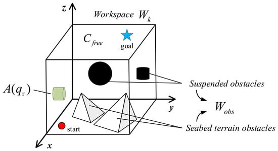
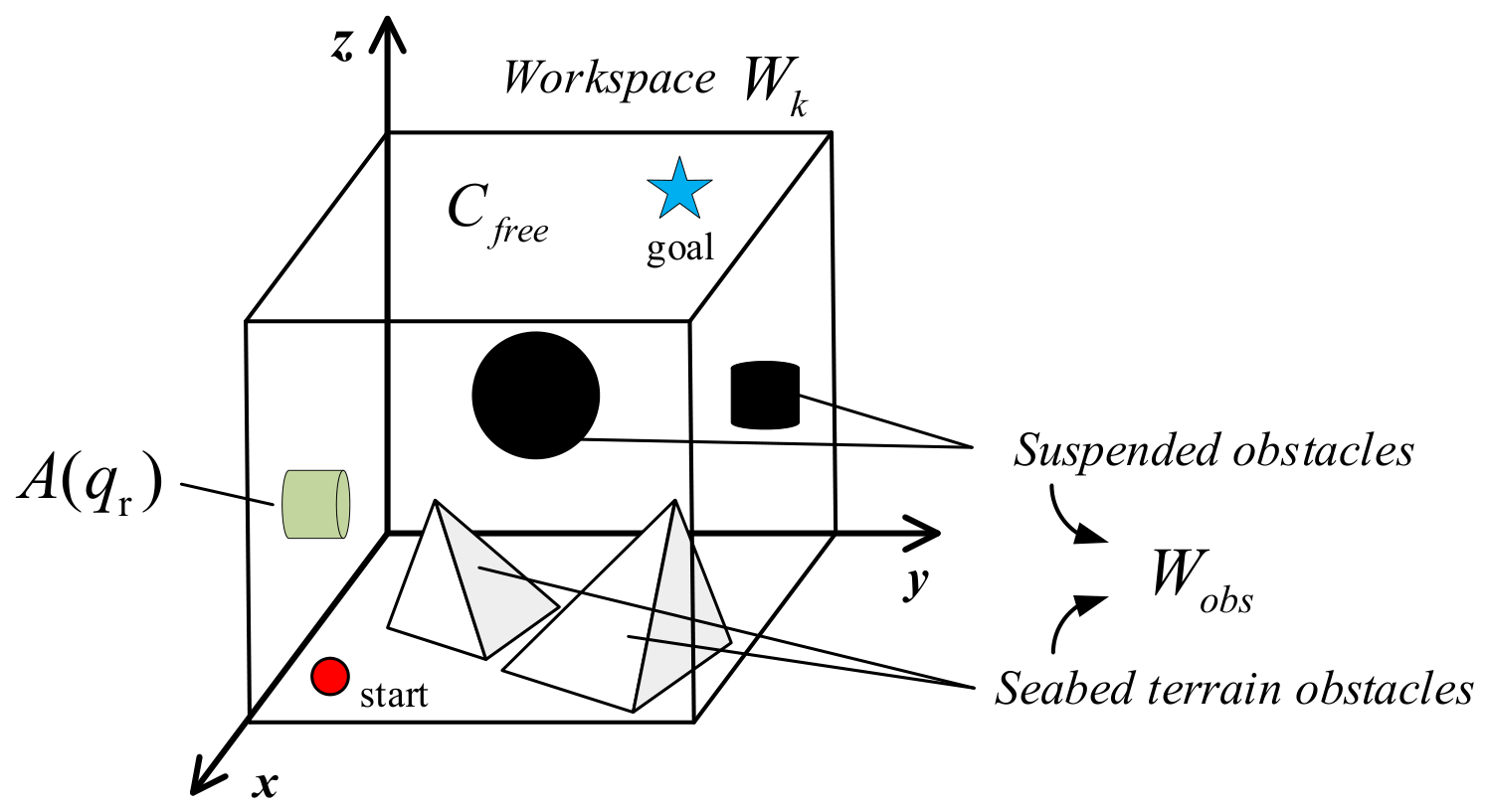
Within W_k, the seabed, reefs, and suspended obstacles are represented by the obstacle set W_obs. A configuration space C_K is introduced to describe all admissible vehicle configurations considered by the planner. The configuration space is partitioned into the collision space C_obs and the free space C_free, as defined in Equations (14) and (15). Figure 2 illustrates the corresponding planning problem.

C_obs = {q_r ∈ C_K|A(q_r) ∩ W_obs) ≠ ∅}

(14)

where q_r is the vehicle configuration vector and A(q_r) denotes the physical region occupied by the vehicle at q_r. A configuration belongs to C_obs when A(q_r) intersects the obstacle set W_obs.

C_free = C_K\C_obs = {q_r ∈ C_K|A(q_r) ∩ W_obs) = ∅}

(15)

Figure 2. Schematic of the three-dimensional path-planning problem. The vehicle must travel from the start configuration to the goal configuration through the collision-free region while avoiding seabed terrain, reefs, and suspended obstacles.

The free space C_free is the complement of C_obs in C_k. Thus, for every q_r ∈ C_free the region occupied by the vehicle does not overlap any environmental obstacle. The planning objective is to determine a continuous collision-free path from the prescribed start configuration x_star to the goal configuration x_goal while minimizing the selected path-cost function. Collision checking is performed on voxelized path segments with an explicit integer-valued clearance radius. This discrete test provides evidence of safety at the tested map resolution, not a continuous-space or uncertain-perception guarantee.

3. Path-Planning and Controller Design

3.1. Development of the iRRT Algorithm

The rapidly exploring random tree (RRT) is a sampling-based planner that incrementally explores a continuous free space to obtain a feasible path. Unlike grid-based search methods, RRT does not require the entire workspace to be discretized in advance. Instead, a search tree is expanded toward randomly generated samples, which makes the method suitable for high-dimensional continuous spaces.

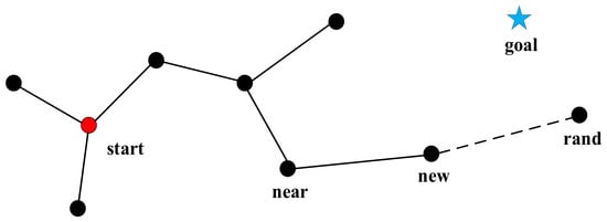
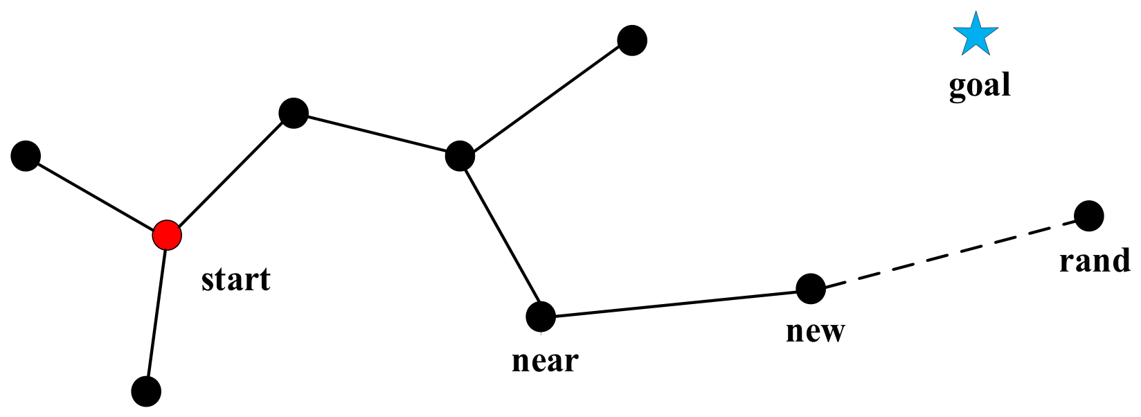
The basic procedure consists of initialization, random sampling, nearest-neighbor search, tree extension, collision checking, and termination when the goal region is reached, as illustrated in Figure 3.

Figure 3. Basic RRT extension. A random sample is drawn in the free space, the nearest tree node is identified, and a collision-free edge is extended toward the sample to generate a new node.

Conventional RRT can produce paths containing redundant waypoints and abrupt directional changes, and its use of a fixed extension step limits its adaptability to spatially varying obstacle density. To address these limitations, a multi-strategy enhanced RRT method is first developed for static planning. A replanning mechanism is then incorporated to handle newly detected obstacles, resulting in the proposed iRRT algorithm.

3.1.1. Multi-Strategy Enhanced RRT Algorithm

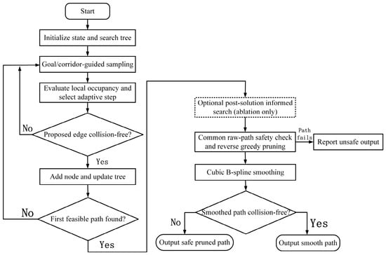
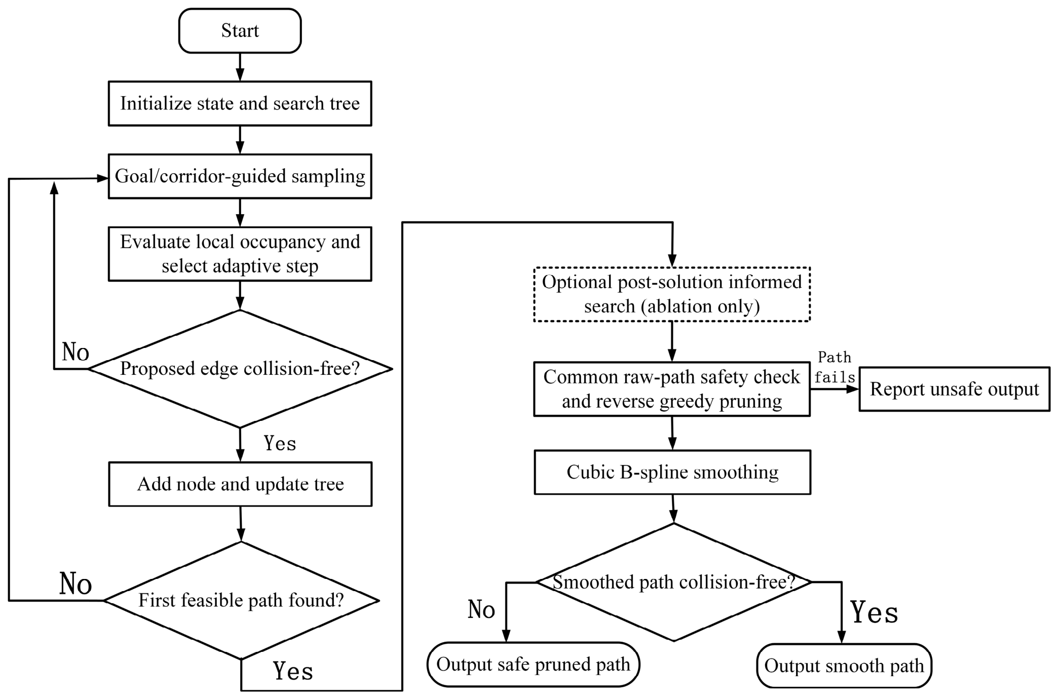
The planner first seeks a feasible collision-checked tree path using guided sampling, a cost-aware parent choice, and local step adaptation. In the four-planner comparisons, the search terminates at the first feasible path. Post-solution ellipsoidal informed sampling is evaluated separately in the equal-budget ablation, where the informed variants allow 1200 additional extension attempts and draw an informed sample with probability 0.8. The nominal step is seven voxels for static planning and five voxels after obstacle insertion. A returned path is subjected to the common radius-aware check, reverse greedy pruning, and collision-checked B-spline smoothing, with the safe pruned path retained if the spline is rejected. Figure 4 summarizes this sequence.

Figure 4. Flowchart of the RRT-based planning and path-refinement procedure. Guided sampling and adaptive extension generate a feasible tree path; a common raw-path check, reverse greedy pruning, and checked B-spline smoothing produce the final output. Post-solution ellipsoidal informed sampling is an optional stage evaluated in the equal-budget ablation.

Once a feasible path is available, an optional post-solution search can limit some samples to the region where the current path cost may be improved. Equations (16)–(19) describe the prolate ellipsoid used in this variant: the start and goal are its foci, and the current best path cost determines its major axis. At each additional iteration, the ellipsoid is sampled with probability 0.8; otherwise, the existing exploration policy is used. This stage is evaluated only in the equal-budget ablation and is disabled in the four-planner comparisons in Table 1 and Table 2.

Table 1. Thirty-run comparison of ACO, A*, RRT, and iRRT on the static voxel map. Values are mean ± sample SD unless shown as counts. Returned denotes a nonempty raw path; Safe denotes a raw path that passed the additional common radius-two voxel-neighborhood test and the subsequent collision-checked postprocessing. Length, turning, and postprocessing-time statistics include safe paths only; planner time covers all 30 planner calls and excludes common postprocessing. A dash (—) means that no safe-path statistic is available. Expansion counters are algorithm-specific diagnostics; direct percentage comparisons of tree expansions are made only between RRT and iRRT. † A* records neighbor evaluations rather than valid tree expansions, so the marked entries are N/A.

Metric	ACO	A*	RRT	iRRT
Search time (s)	8.755 ± 0.266	19.145 ± 0.521	0.047 ± 0.027	0.049 ± 0.032
Path length (voxel)	—	459.41 ± 0.00	483.32 ± 22.42	475.03 ± 10.96
Number of discrete path nodes	405.1 ± 3.2	351.0 ± 0.0	102.9 ± 12.6	64.4 ± 4.8
Total expanded nodes	4,480,575 ± 19,492	257,245 ± 0	953 ± 577	638 ± 403
Valid expanded nodes	3,819,498 ± 14,313	N/A †	596 ± 346	331 ± 194
Valid expansion ratio	0.852 ± 0.001	N/A †	0.635 ± 0.074	0.530 ± 0.044
Maximum turning angle (°)	—	35.5 ± 0.0	8.7 ± 7.2	9.1 ± 5.6
Number of turns exceeding 45°	—	0.00 ± 0.00	0.00 ± 0.00	0.00 ± 0.00
Returned paths/30	30/30	30/30	30/30	30/30
Safe paths/30	0/30	30/30	30/30	30/30
B-spline accepted/30	0/30	30/30	30/30	30/30
Postprocessing time, safe runs (s)	—	0.294 ± 0.009	0.061 ± 0.021	0.045 ± 0.008

Table 2. Thirty-run comparison of the four algorithms after introduction of the fixed cylindrical obstacle. The definitions, additional radius-two test, and mean ± sample SD convention follow Table 1. All four planners returned nonempty raw paths. A dash (—) for a safe-path metric means that no returned path passed the additional common test; it does not mean that the planner failed to return a path. Planner time excludes common postprocessing. Expansion counters are algorithm-specific; † the A* neighbor-evaluation entries are N/A under the valid-tree-expansion labels. This fixed-obstacle experiment is separate from the moving-obstacle stress test.

Metric	ACO	A*	RRT	iRRT
Search time (s)	7.612 ± 0.362	2.259 ± 0.158	0.025 ± 0.010	0.030 ± 0.015
Path length (voxel)	—	—	297.74 ± 22.08	295.52 ± 17.56
Number of discrete path nodes	224.2 ± 2.5	207.0 ± 0.0	60.0 ± 8.1	52.3 ± 5.7
Total expanded nodes	2,836,378 ± 28,134	28,090 ± 0	539 ± 236	504 ± 253
Valid expanded nodes	2,375,579 ± 21,029	N/A †	366 ± 149	269 ± 124
Valid expansion ratio	0.838 ± 0.001	N/A †	0.689 ± 0.060	0.544 ± 0.058
Maximum turning angle (°)	—	—	13.0 ± 9.8	14.8 ± 15.4
Number of turns exceeding 45°	—	—	0.00 ± 0.00	0.03 ± 0.18
Returned paths/30	30/30	30/30	30/30	30/30
Safe paths/30	0/30	0/30	30/30	30/30
B-spline accepted/30	0/30	0/30	30/30	29/30
Postprocessing time, safe runs (s)	—	—	0.026 ± 0.009	0.024 ± 0.009

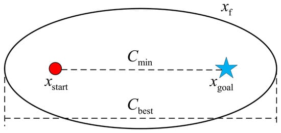
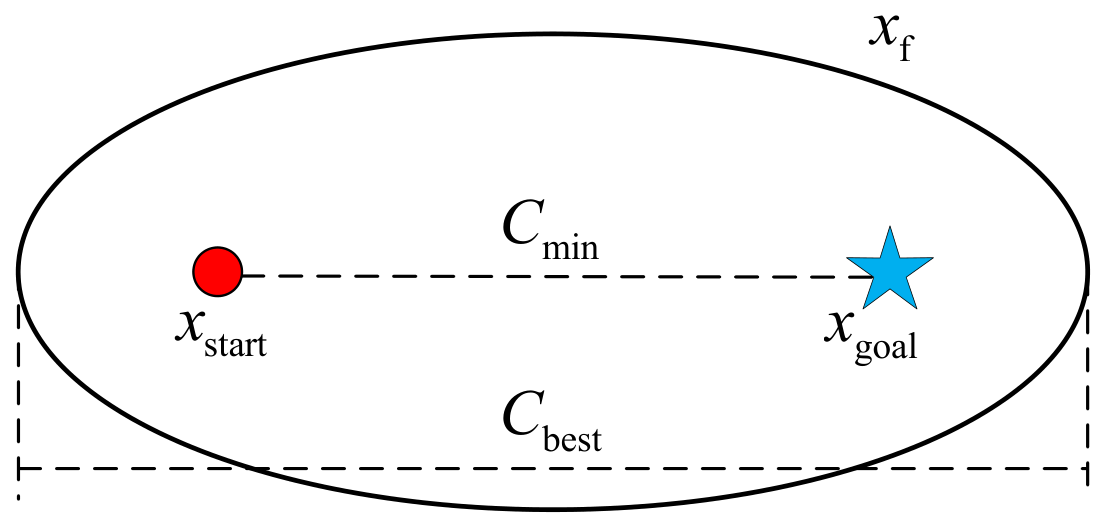
Let C_best denote the cost of the current best path and C_min denote the Euclidean distance between the start and goal configurations. Any sample that can improve the current solution must satisfy the combined-distance condition in Equation (16). The corresponding effective sampling set has x_start and x_goal as its two focal points.

$$x_{\mathrm{f}}=\left\{x_{\mathrm{s}}\in C_{\mathrm{K}}{\left|‖x_{\mathrm{s}}-x_{\mathrm{start}}‖\right.}_2+{‖x_{\mathrm{s}}-x_{\mathrm{goal}}‖}_2\le C_{\mathrm{best}}\right\}$$

(16)

Figure 5 illustrates the ellipsoidal region used only in the optional post-solution informed-search ablation.

Figure 5. Ellipsoidal informed-sampling region. The start and goal configurations are the focal points, and the sampling region contracts as the current best path cost approaches the theoretical lower bound. This post-solution sampling stage is used only in the optional informed-search ablation.

Uniform samples in a unit ball are mapped to the ellipsoidal region through an affine transformation. The diagonal entries of the scaling matrix L define the semi-axis lengths, with the major axis aligned with the start-to-goal direction and the remaining axes orthogonal to it:

$$L_{\mathrm{C}}=\mathrm{diag}\left({\displaystyle \frac{C_{\mathrm{best}}}{2}},{\displaystyle \frac{\sqrt{C_{\mathrm{best}}^2-C_{\min }^2}}{2}},{\displaystyle \frac{\sqrt{C_{\mathrm{best}}^2-C_{\min }^2}}{2}}\right)$$

(17)

When C_best is much larger than C_min, the ellipsoid is relatively broad. As C_best approaches C_min, the minor axes shrink, and the sampling region concentrates around the current best solution. A sample in the ellipsoid is generated by

q_rand = C_RL_Cq_ball + q_center

(18)

where q_ball is uniformly distributed in the unit ball, q_center is the ellipsoid center, and C_R is the rotation matrix that aligns the major axis with the start-to-goal direction. Samples falling inside obstacles are rejected. The ellipsoid volume is given by

$$\mathit{Vol}(x_{\mathrm{f}})={\displaystyle \frac{\pi }{6}}\cdot C_{\mathrm{best}}\cdot \left(C_{\mathrm{best}}^2-C_{\min }^2\right)$$

(19)

The ellipsoid limits a fraction of post-solution samples to points that could improve the current path cost under the Euclidean lower bound. This is a search-domain restriction, not a guarantee of shorter paths or faster execution in a finite-budget experiment; its isolated effect is therefore evaluated by the ablation in Section 4.1. Second, obstacles in complex nearshore environments are generally distributed non-uniformly. A large fixed extension step may cause an edge to cross an obstacle or bypass a narrow passage, whereas a small step reduces search efficiency in open regions. An environment-aware adaptive step-size strategy is therefore introduced. The occupied-voxel fraction Ω(x_s) is calculated in a local neighborhood of the current tree node x_s, as defined in Equation (20).

$$\mathsf{\Omega }\left(x_{\mathrm{s}}\right)={\displaystyle \frac{1}{N_f}}{\displaystyle \sum _{i=1}^{N_f}\chi \left(f_i\in W_{\mathrm{obs}}\right)}$$

(20)

where x_s is the current tree node, N_f is the number of inspected voxels in its radius-three neighborhood, f_i is the ith inspected voxel, W_obs is the occupied-voxel set, and χ(⋅) is one when its argument is true and zero otherwise. Thus, Ω(x_s) is the local occupied-voxel fraction. The nominal step is then adapted according to Equation (21).

$$\delta =\left\{\begin{array}{cc}\mathrm{round}(0.45{\mathsf{\rho }}_{\mathrm{base}}),\hfill & \mathsf{\Omega }\left(x_{\mathrm{s}}\right)>0.07,\hfill \\ \mathrm{round}(1.35{\mathsf{\rho }}_{\mathrm{base}}),\hfill & \mathsf{\Omega }\left(x_s\right)<0.015 \mathrm{and} d\left(x_s,x\_g\right)>70,\hfill \\ {\mathsf{\rho }}_{\mathrm{base}},\hfill & \mathrm{otherwise}.\hfill \end{array}\right.$$

(21)

where δ is the selected extension step, ρ_base is the nominal step, and d(x_s,x_g) is the Euclidean distance from the current node to the goal. The fixed thresholds 0.07 and 0.015 distinguish high and low local occupancy. For the reported runs, ρ_base is seven voxels on the static map and five voxels after obstacle insertion. The implementation also clips the rounded step to the admissible map range and subsequently checks each proposed edge against the updated occupancy map.

Third, the raw path generated by conventional RRT generally contains numerous short segments and redundant waypoints. Abrupt changes in tangent direction can also increase the tracking burden on the controller. A two-stage postprocessing procedure comprising reverse greedy pruning and cubic B-spline smoothing is therefore applied. The smoothed curve is subsequently sampled at the controller sampling interval to generate the reference-position sequence.

Reverse greedy pruning is first used to simplify the path topology. Based on the triangle inequality, multiple short segments are replaced by the longest available collision-free segment. Let P_p = {q₁,q₂,⋯,q_n} denote the original waypoint sequence, with q₁ = x_start and q_n = x_goal. The objective is to obtain an ordered subset containing fewer waypoints while ensuring that each segment between adjacent retained waypoints passes the radius-aware sampled collision test C_free. The initial anchor point is set to q₁, and the visibility between the anchor and each subsequent waypoint is evaluated using Equation (22).

$$\mathrm{Vis}(q_i,q_j)=\left\{\begin{array}{cc}1,\hfill & \left(1-\mu \right)q_i+\mu q_j\in C_{\mathrm{free}}, \forall \mu \in \left[0,1\right]\hfill \\ 0,\hfill & \mathit{otherwise}\hfill \end{array}\right.$$

(22)

where q_i and q_j are two waypoints in the configuration space, and μ is the interpolation parameter used for line-of-sight collision checking. Subject to this visibility constraint, the next retained waypoint is selected according to the maximum-span criterion in Equation (23).

$$q_{\mathrm{next}}=\underset{q_k\in P_{\mathrm{p}}}{\mathrm{argmax}\left\{k\left|\mathrm{Vis}\left(q_{\mathrm{anchor}},q_k\right)\right.=1\right\}}$$

(23)

After q_next is selected, it is added to the pruned waypoint set and becomes the new anchor point. This procedure is repeated until the goal is reached. The triangle inequality in Equation (24) shows that replacing several short segments with a direct collision-free segment cannot increase the path length and reduces the number of waypoints.

$${‖q_i-q_k‖}_2\le {‖q_i-q_j‖}_2+{‖q_j-q_k‖}_2$$

(24)

The pruned waypoint set is then used as the control polygon of a cubic B-spline. Let P_∗ = {p₀,p₁,⋯,p_n}, where p₀ and p_n are the start and goal points, respectively. The cubic B-spline curve is defined as a weighted combination of the basis functions in Equation (25).

$$S\left(u_{\mathrm{p}}\right)={\displaystyle \sum _{i=0}^n{p}_i{N}_{i,3}\left(u_{\mathrm{p}}\right)},u_{\mathrm{p}}\in \left[u_{\mathrm{p}\min },u_{\mathrm{p}\max }\right]$$

(25)

where S(u_p) is the cubic B-spline curve, u_p is the curve parameter, and N_i,3(u_p) is the cubic B-spline basis function.

Reverse greedy pruning retains the farthest waypoint reachable from the current anchor by a collision-free straight segment. A cubic B-spline is then sampled from the pruned control polygon at a target spacing of 0.75 voxels. The smoothed candidate is accepted only when every sampled segment passes the same collision-clearance test; otherwise, the safe pruned polyline is returned. Consequently, spline acceptance is reported separately from path safety in the Results. Spline smoothing alone is not treated as a collision-avoidance method.

3.1.2. Obstacle-Triggered Replanning Mechanism

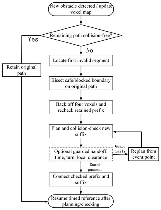
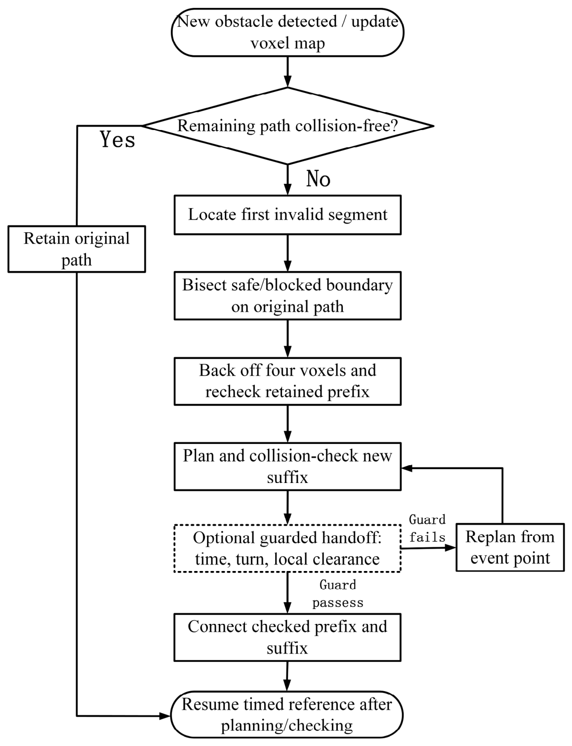
A path planned from prior map information may become invalid when a previously unknown obstacle is detected during execution. In this study, this event is described as the appearance of a newly detected obstacle. An obstacle-triggered replanning mechanism is therefore applied when the occupancy map is updated. Segment checks on the remaining path locate the first conflict, and path-domain bisection determines a candidate safe rollback point while retaining as much of the valid original route as possible.

After a new obstacle is inserted, the occupancy map is updated, and the untraversed part of the original path is checked segment by segment. For points a and b on one segment, define the radius-aware collision indicator as follows:

$$C_r(a,b;M)=\left\{\begin{array}{cc}1,\hfill & \mathrm{if} \mathrm{the} \mathrm{segment} a\to b \mathrm{is} \mathrm{collision}\text{-}\mathrm{free} \mathrm{at} \mathrm{clearance} r,\hfill \\ 0,\hfill & \mathrm{otherwise}.\hfill \end{array}\right.$$

(26)

where M is the updated occupancy map and r is the integer voxel-neighborhood radius used for the segment test. A value of one means that all sampled positions along the segment pass the test; a value of zero means that at least one fails.

At the event position, the untraversed path is split into its remaining edges. A conflict is present when at least one such edge fails the radius-aware test:

$$I_e=1-{\displaystyle \prod _{e\in {\mathcal{E}}_{\mathrm{rem}}}{C}_r}(e;M_e)$$

(27)

where $ℰ$_rem is the set of untraversed path edges and M_e is the map after the obstacle event. Thus, I_e = 1 when at least one untraversed edge is invalid. The first failed edge is then used to locate the handoff point by bisection.

A point within the first failed edge is parameterized by α:

q(α) = p_j + α(p_j+1 − p_j),  0 ≤ α ≤ 1

(28)

The safe-side and blocked-side parameter bounds are denoted by α_L and α_U. At each iteration, the midpoint is checked from the safe start of the edge:

$${\alpha }_m={\displaystyle \frac{{\alpha }_L+{\alpha }_U}{2}},\hspace{1em}\hspace{1em}\left\{\begin{array}{cc}{\alpha }_L\leftarrow {\alpha }_m,\hfill & C_r(p_j,q({\alpha }_m);M_e)=1,\hfill \\ {\alpha }_U\leftarrow {\alpha }_m,\hfill & C_r(p_j,q({\alpha }_m);M_e)=0.\hfill \end{array}\right.$$

(29)

The bisection stops when the unresolved arclength on this edge is at most 0.25 voxels:

(α_U − α_L)‖p_j+1 − p_j‖ ≤ 0.25 voxels

(30)

The last safe boundary estimate is moved backward by four voxels along the original path. The selected replanning arclength cannot precede the event location:

s_r = max{s_e, s_j + α_L‖p_j+1 − p_j‖ − 4 voxels}

(31)

Before reusing the retained prefix, every one of its edges is checked again on the updated map:

C_r(q_i,q_i+1;M_e) = 1,  ∀i ∈ $ℐ$_prefix

(32)

where p_j and p_j+1 bound the first failed edge, α_L and α_U bracket its safe and blocked sides, and s_e and s_j are the original-path arclengths at the event and at p_j, respectively. The selected rollback point is no earlier than the event position. Each edge (q_i,q_i+1) of the retained prefix is rechecked on M_e before it is reused.

The integrated tests use a four-voxel planning clearance. This procedure identifies a checked old-path prefix and a candidate connection location; the ability of the regenerated path to be tracked safely is assessed separately. In the guarded handoff extension, a candidate is also rejected if its connection turn exceeds 75° or the first six voxels fail a radius-five test. Prefix reuse is limited by a 0.4 s planning-time budget, and a rejected candidate falls back to replanning from the event position. Vehicle motion is held until planning and checks finish. These additional guards are evaluated on held-out seeds 61–90 rather than assumed to improve every event. The overall obstacle-triggered replanning procedure is illustrated in Figure 6.

Figure 6. Flowchart of obstacle-triggered replanning on the updated voxel map. The first invalid path segment is located before path-domain bisection, safety backoff, prefix verification, and new-suffix checking. The dashed guarded-handoff branch denotes the separately evaluated connection policy; a rejected candidate is replanned from the event position.

3.2. Cascaded Translational MPC–PID Controller with Residual Disturbance Estimation

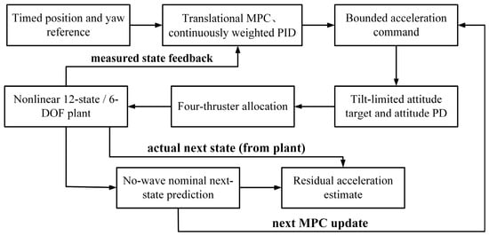
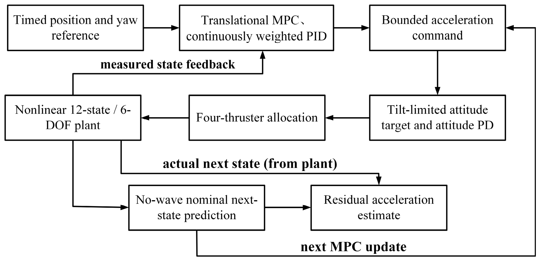
The path planner supplies a timed position and yaw reference. A translational MPC outer loop computes a desired inertial acceleration, and a continuously weighted PID term provides additional tracking correction. The desired force is converted into a tilt-limited attitude command; an inner attitude PD loop and bounded four-thruster allocation drive the nonlinear 12-state plant. A residual estimator compares the measured state transition with a no-wave nominal prediction and supplies an acceleration estimate to the next MPC prediction. Figure 7 shows these signal paths.

Figure 7. Cascaded trajectory-tracking architecture used in the simulations. Translational MPC and continuously weighted PID generate a bounded acceleration request; attitude PD and four-thruster allocation drive the nonlinear six-degree-of-freedom plant. Actual and no-wave nominal state transitions form a residual acceleration estimate for the next MPC prediction.

3.2.1. MPC Controller

The simulated plant retains all six degrees of freedom, but the outer MPC predicts only translational position and inertial-frame velocity. Its six-dimensional prediction state and three-dimensional output are

$$z_k={\left[\begin{array}{cc}{p}_k^{\mathrm{T}}& v_{N,k}^{\mathrm{T}}\end{array}\right]}^{\mathrm{T}},\hspace{1em}\hspace{1em}{y}_k=\left[\begin{array}{cc}{I}_3& 0_3\end{array}\right]z_k$$

(33)

For a sampling period T_s = 0.2 s, commanded inertial acceleration a_k enters a discrete double-integrator approximation:

$$z_{k+1}=\left[\begin{array}{cc}{I}_3& T_s{I}_3\\ 0_3& I_3\end{array}\right]z_k+\left[\begin{array}{c}\frac{1}{2}{T}_s^2{I}_3\\ T_s{I}_3\end{array}\right]a_k$$

(34)

where p_k and v_N,k are position and inertial-frame velocity, z_k is the six-dimensional outer-loop prediction state, and y_k selects its three position entries. The matrices in Equation (34) are a discrete double-integrator approximation with T_s = 0.2 s; the nonlinear six-degree-of-freedom plant remains the simulation model used to evaluate tracking.

The output predictions are stacked for 12 samples. When residual disturbance estimation is active, the current estimated acceleration is repeated across the prediction sequence:

$$Y=\mathsf{\Phi }{z}_k+\mathsf{\Gamma }\left[U+\left({\mathbf{1}}_{12}\otimes {\widehat{d}}_k\right)\right]$$

(35)

The unconstrained quadratic objective penalizes position tracking error and the acceleration sequence:

$$\begin{array}{c}J={(Y-Y_{\mathrm{ref}})}^{\mathrm{T}}\overline{Q}(Y-Y_{\mathrm{ref}})+U^{\mathrm{T}}\overline{\mathit{R}}U,\hfill \\ Q=\mathrm{diag}(12,12,16),\hspace{1em}\hspace{1em}\mathit{R}=0.4I_3.\hfill \end{array}$$

(36)

The sequence is obtained by a regularized linear-system solve; only the first three components are used at the current update:

$$\begin{array}{c}H={\mathsf{\Gamma }}^{\mathrm{T}}\overline{Q}\mathsf{\Gamma }+\overline{\mathit{R}}+{10}^{-7}I,\hfill \\ U^{*}=-H^{-1}{\mathsf{\Gamma }}^{\mathrm{T}}\overline{Q}\left[\mathsf{\Phi }{z}_k+\mathsf{\Gamma }({\mathbf{1}}_{12}\otimes {\widehat{d}}_k)-Y_{\mathrm{ref}}\right].\hfill \end{array}$$

(37)

where U stacks 12 future three-axis acceleration commands, Y stacks their predicted positions, Φ and Γ are the lifted prediction matrices, and ${\widehat{d}}_k$ is the current three-axis residual acceleration estimate repeated over the horizon. In the objective, $\overline{Q}$ and $\overline{R}$ are block-diagonal matrices formed from Q and R, while Y_ref is the timed position reference. The regularization term in H is 10⁻⁷ I. MATLAB R2024b (The MathWorks, Inc., Natick, MA, USA) solves the linear system and applies only the first acceleration command; the subsequent componentwise saturation is outside the quadratic optimization.

The 12-step acceleration sequence is computed by MATLAB matrix left division rather than by a constrained quadratic-programming solver. Only the first three-axis acceleration command is applied, and it is clipped componentwise to ±0.8 m/s² after the solve. It is converted to a desired inertial force using nominal mass and drag compensation; the horizontal force is then limited to a 30° tilt. An attitude PD loop tracks the resulting orientation, with moment limits of ±[3, 3, 0.4] N·m and individual thruster-force limits of 0–25 N. These limits act on the applied command or downstream actuators rather than entering the horizon optimization. Thus, the implemented controller uses unconstrained receding-horizon predictive optimization followed by saturation: clipping bounds the applied signals, but it does not guarantee feasibility of the unexecuted predicted sequence or preserve the unconstrained optimum after clipping.

3.2.2. Nearshore Wave-Disturbance Model and Residual Estimation

Wave-induced loads introduce time-varying disturbances into the vehicle dynamics and can excite oscillatory motion in both the horizontal and vertical directions [39,40]. A finite-depth free-surface elevation proxy is constructed from a JONSWAP-shaped spectral weight [41], with the finite-depth correction based on the TMA spectral formulation [42]. The peak frequency and piecewise spectral width are defined as follows:

$$\begin{array}{c}{\omega }_p={\displaystyle \frac{2\pi }{T_p}},\hfill \\ {\sigma }_i=\left\{\begin{array}{cc}0.07,\hfill & {\omega }_i\le {\omega }_p,\hfill \\ 0.09,\hfill & {\omega }_i>{\omega }_p,\hfill \end{array}\right.\hfill \\ S_J({\omega }_i)={\omega }_i^{-5}\exp \left[-1.25{\left({\displaystyle \frac{{\omega }_p}{{\omega }_i}}\right)}^4\right]{\gamma }^{\exp \left[-{\displaystyle \frac{1}{2}}{\left({\displaystyle \frac{{\omega }_i-{\omega }_p}{{\sigma }_i{\omega }_p}}\right)}^2\right]}.\hfill \end{array}$$

(38)

where T_p is the peak period, ω_p the peak angular frequency, ω_i the angular frequency of component i, σ_i the piecewise spectral width, and γ the peak-enhancement factor. The JONSWAP-shaped function S_J provides relative spectral weights before finite-depth correction and normalization.

Finite depth is represented through the dispersion relation and depth transfer factor. The discrete spectrum is then normalized to variance (H_s/4)²:

$$\begin{array}{c}{\omega }_i^2=g{k}_i\tanh (k_{i}h),\hfill \\ F_h({\omega }_i)={\displaystyle \frac{{\tanh }^2(k_{i}h)}{1+2k_{i}h/\sinh (2k_{i}h)}},\hfill \\ S_i={\displaystyle \frac{S_J({\omega }_i)F_h({\omega }_i){(H_s/4)}^2}{{\displaystyle \sum _j{S}_J}({\omega }_j)F_h({\omega }_j)\Delta \omega }}.\hfill \end{array}$$

(39)

where k_i is the wave number obtained from the finite-depth dispersion relation, h is water depth, F_h is the depth-transfer factor, H_s is significant wave height, and Δω is the frequency increment. The normalized discrete spectral density S_i gives a total elevation variance of approximately ${(H_s/4)}^2$ over the selected components.

Independent seeded phases are assigned to components between 0.25 and 3.0 rad/s. The time-domain elevation proxy is

$$\begin{array}{c}{A}_i=\sqrt{2S_i\Delta \omega },\hfill \\ \eta (t)={\displaystyle \sum _{i=1}^{64}{A}_i}\cos ({\omega }_{i}t+{\varphi }_i)\hfill \end{array}$$

(40)

The simulated force is an explicitly chosen equivalent acceleration mapping in a fixed direction, rather than an identified hydrodynamic wave-load transfer function:

$$\begin{array}{c}{e}_w={\displaystyle \frac{{[1,-0.6,0.3]}^{\mathrm{T}}}{\Vert {[1,-0.6,0.3]}^{\mathrm{T}}\Vert }},\hfill \\ a_w(t)=0.5\eta (t)e_w,\hfill \\ F_w(t)=\overline{m}{a}_w(t).\hfill \end{array}$$

(41)

where A_i is component amplitude and ϕ_i is an independently seeded phase. The resulting elevation η(t) is converted to a prescribed inertial-frame acceleration a_w(t) along the unit direction e_w; $\overline{m}$ is the mean of the three effective translational masses used to express an equivalent force F_w(t). The coefficient 0.5 has units s⁻² in this mapping. This is a reproducible disturbance proxy, not an identified wave-load transfer function. The component frequencies are not modified by vehicle speed or encounter angle.

The simulations use H_s = 1 m, T_p = 6 s, h = 12 m, γ = 3.3, and the mean effective translational mass $\overline{m}$ in the force conversion.

At each update, the same command is applied once to the actual disturbed plant and once to a no-wave nominal model. The difference in next-step inertial velocities gives a residual acceleration:

$$d_{\mathrm{res},k}={\displaystyle \frac{v_{N,k+1}-v_{N,k+1}^0}{T_s}}$$

(42)

A first-order filter updates the disturbance estimate available at the next MPC step:

$${\widehat{d}}_{k+1}={\widehat{d}}_k+0.55\left(d_{\mathrm{res},k}-{\widehat{d}}_k\right)$$

(43)

where v_N,k+1 is the actual next-step inertial velocity and $v_{N,k+1}^0$ is the nominal no-wave prediction under the same applied command. Their difference divided by T_s defines a residual acceleration. The estimate ${\widehat{d}}_{k+1}$ is updated with fixed gain 0.55 and enters the next MPC prediction.

The known injected wave signal is logged for validation but is not supplied to the estimator. The estimator uses the actual-minus-nominal state transition rather than a Luenberger observer of individual wave states. The numerical study assumes noiseless access to all 12 plant states; partial and noisy sensing are not evaluated.

3.2.3. PID Compensation and Control-Input Fusion

The PID correction uses next-sample position error, reference-minus-actual inertial velocity error, and a clipped integral state:

$$\begin{array}{c}{e}_k=p_{\mathrm{ref},k+1}-p_k,\hspace{1em}\hspace{1em}\hfill \\ e_{v,k}=v_{\mathrm{ref},k+1}-v_{N,k},\hfill \\ I_k=\mathrm{clip}(I_{k-1}+T_s{e}_k,-2,2),\hfill \\ a_{\mathrm{PID},k}=K_p\odot e_k+K_d\odot e_{v,k}+K_i\odot I_k.\hfill \end{array}$$

(44)

The MPC and PID acceleration commands are combined with an error-dependent continuous weight:

$$\begin{array}{c}{\alpha }_k=0.25\min \left(1,{\displaystyle \frac{\Vert e_k\Vert }{0.5}}\right),\hfill \\ a_{\mathrm{cmd},k}=\mathrm{clip}\left(a_{\mathrm{MPC},k}+{\alpha }_k{a}_{\mathrm{PID},k},-0.8,0.8\right).\hfill \end{array}$$

(45)

where e_k, e_v,k, and I_k are the position, inertial-velocity, and clipped integral errors, respectively; K_p = [1.4,1.4,1.8]^T, K_i = [0.02,0.02,0.02]^T, and K_d = [1.7,1.7,1.8]^T are the PID gains; and ⊙ denotes componentwise multiplication. The nonnegative weight α_k varies continuously with position error and scales the PID correction before the commanded acceleration is clipped to ±0.8 m/s² per axis. It is not a binary PID switch. The residual disturbance estimate enters the MPC prediction in Equation (35), rather than being subtracted directly from a thruster force.

3.3. Numerical Configuration and Reproducibility

Supplementary Tables S1 and S2 provide the planning, collision-checking, vehicle, controller, and wave-proxy settings used in the numerical study. The original four-planner comparison uses a 500³ voxel map, whereas the controlled environment suite uses 120 × 120 × 50 voxel maps. Planner-only path lengths are measured in voxels; the conversion of 0.1 m/voxel applies to the separate six-degree-of-freedom tracking replay. Each controller comparison uses matched reference paths and seeded wave phases. Returned paths, paths passing the additional radius-two voxel-neighborhood test, and accepted B-splines are counted separately. Reported dispersions are sample standard deviations over 30 runs.

Computation used MATLAB R2024b on 64-bit Windows 10 Pro with an Intel Core i5-12400F CPU and 15.82 GiB of RAM. The MPC sequence is solved by MATLAB matrix left division; no external QP solver is used. Measured controller-update times exclude plotting and event replanning and do not establish a hardware real-time guarantee.

4. Simulation Results and Discussion

The proposed iRRT planner and MPC–PID composite controller were evaluated in a three-dimensional voxel environment constructed in MATLAB. The map included seabed undulations, reefs, suspended obstacles, and newly introduced obstacles to represent a complex nearshore setting. Path-planning performance was evaluated using search time, path length, number of discrete path nodes, total and valid expanded nodes, valid expansion ratio, maximum turning angle, and number of turns exceeding 45°. To assess repeated-run reliability and postprocessing safety, returned paths, paths passing the additional common collision test, accepted B-splines, and postprocessing time are also recorded. Thirty seeded runs are used for each planning scenario. The static and replanned paths are then used to compare PID, MPC, MPC–PID, and MPC–PID with residual disturbance estimation by RMSE, maximum, mean, terminal, and steady-state position errors.

4.1. Path-Planning Simulation

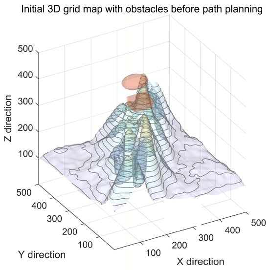
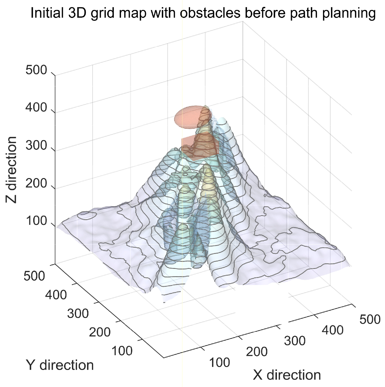
The three-dimensional voxel map in Figure 8 contains representative nearshore seabed features and obstacles. Static planning uses this map without an added event obstacle. For the suddenly obstructed case, one fixed cylinder is inserted along the original route before the four planners are restarted from the same valid position. A separate continuously moving-obstacle experiment is used only as an additional stress test.

Figure 8. Three-dimensional voxel map used for the original planning comparison. Seabed undulations, reefs, and suspended obstacles define the static environment; a fixed cylinder is inserted for the suddenly obstructed scenario. Colors are used to visually distinguish the terrain and obstacle geometries.

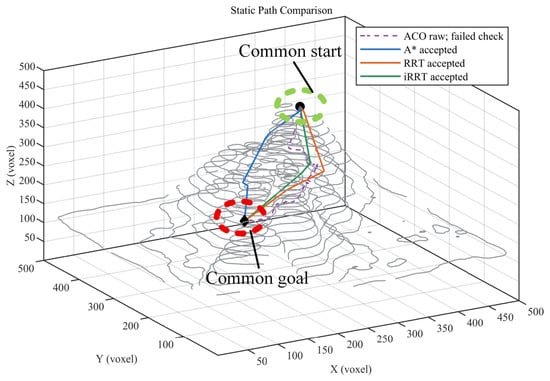
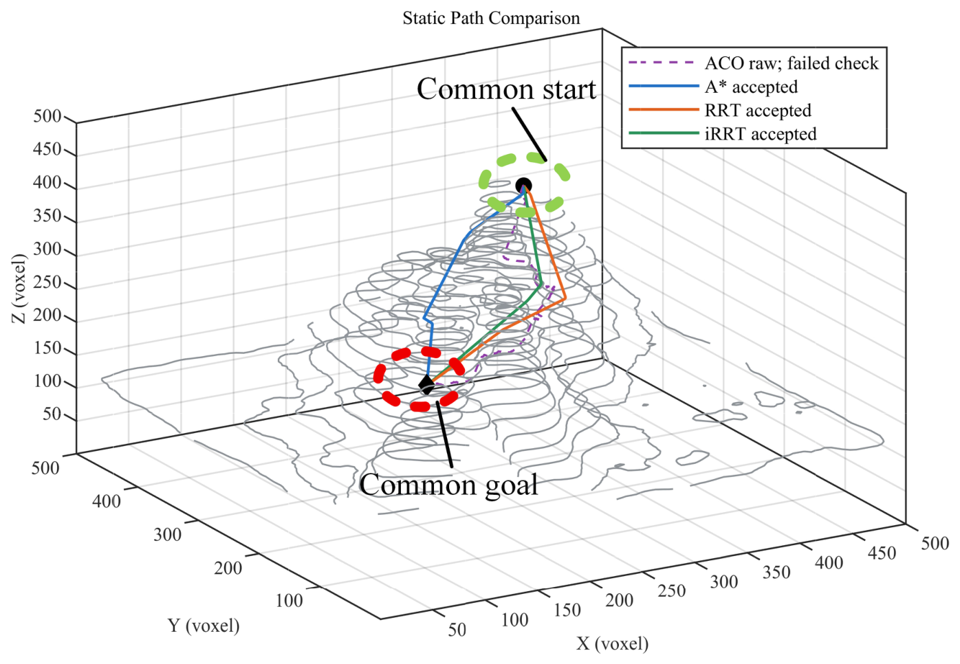
For static planning, identical start and goal points were assigned to ACO, A*, RRT, and iRRT. Figure 9 retains the original four-algorithm route view on the same map and shows the paths from seed 1. The ACO raw route is drawn with a dashed line because it did not pass the additional common radius-two voxel-neighborhood test; it is shown only to illustrate search geometry. The A*, RRT, and iRRT routes passed this test and were refined using the same collision-checked postprocessing. The two tree planners form comparatively compact final routes, while A* gives the shortest safe path in this fixed map. Their repeated-run measures are compared in Table 1.

Figure 9. Representative static-map routes for ACO, A*, RRT, and iRRT at seed 1. Solid lines denote paths accepted after the common radius-two voxel-neighborhood test and collision-checked postprocessing; the dashed ACO line is an illustrative raw output that failed this additional test. Table 1 provides the 30-run measures.

The thirty-run static-map results are summarized in Table 1. All four algorithms returned a raw path in every run; however, none of the ACO raw paths passed the additional common radius-two test, so no safe-path length or turning-angle statistic is assigned to ACO. Among the accepted outputs, A* produced the shortest mean path (459.41 voxels), followed by iRRT (475.03 ± 10.96 voxels) and RRT (483.32 ± 22.42 voxels). Relative to RRT, iRRT’s mean safe-path length was 1.7% lower, but the paired seed-bootstrap interval for their length difference included zero. The iRRT path contained 37.4% fewer raw discrete nodes (64.4 versus 102.9), and its tree expanded 33.1% fewer nodes (638 versus 953). Their mean planner times were nearly the same (0.049 versus 0.047 s), whereas their maximum turning angles were also similar (9.1° versus 8.7°). Thus, the clearest improvement relative to the conventional RRT in this map is a more compact route and tree, rather than a demonstrated shortest-path, fastest-search, or smallest-turning-angle advantage over all methods.

The static comparison therefore motivates a separate check of whether similar route compactness is retained when the original path is interrupted by a newly introduced obstacle.

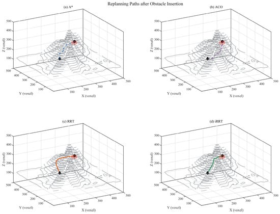
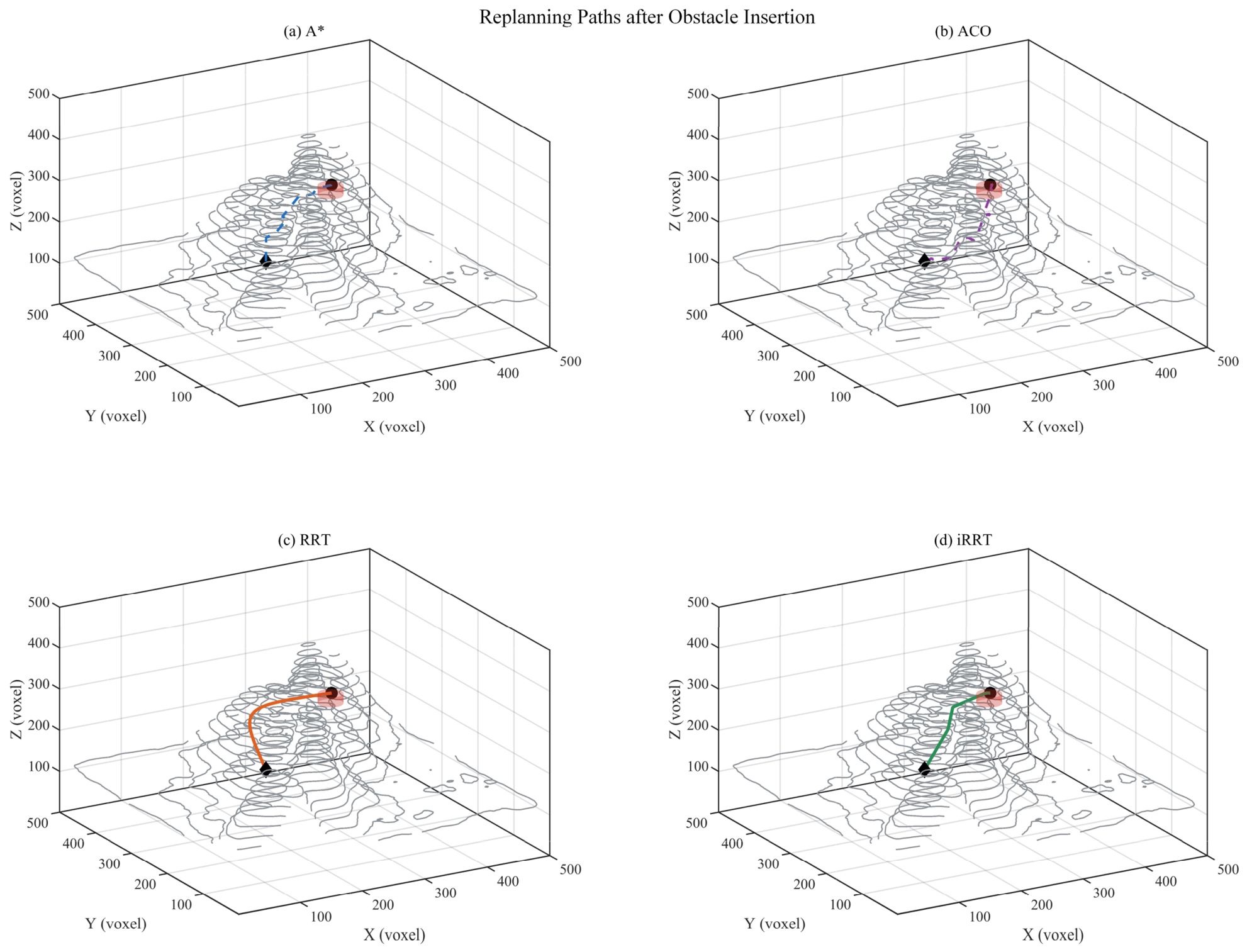
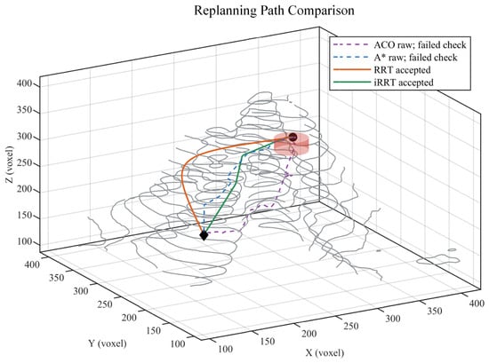
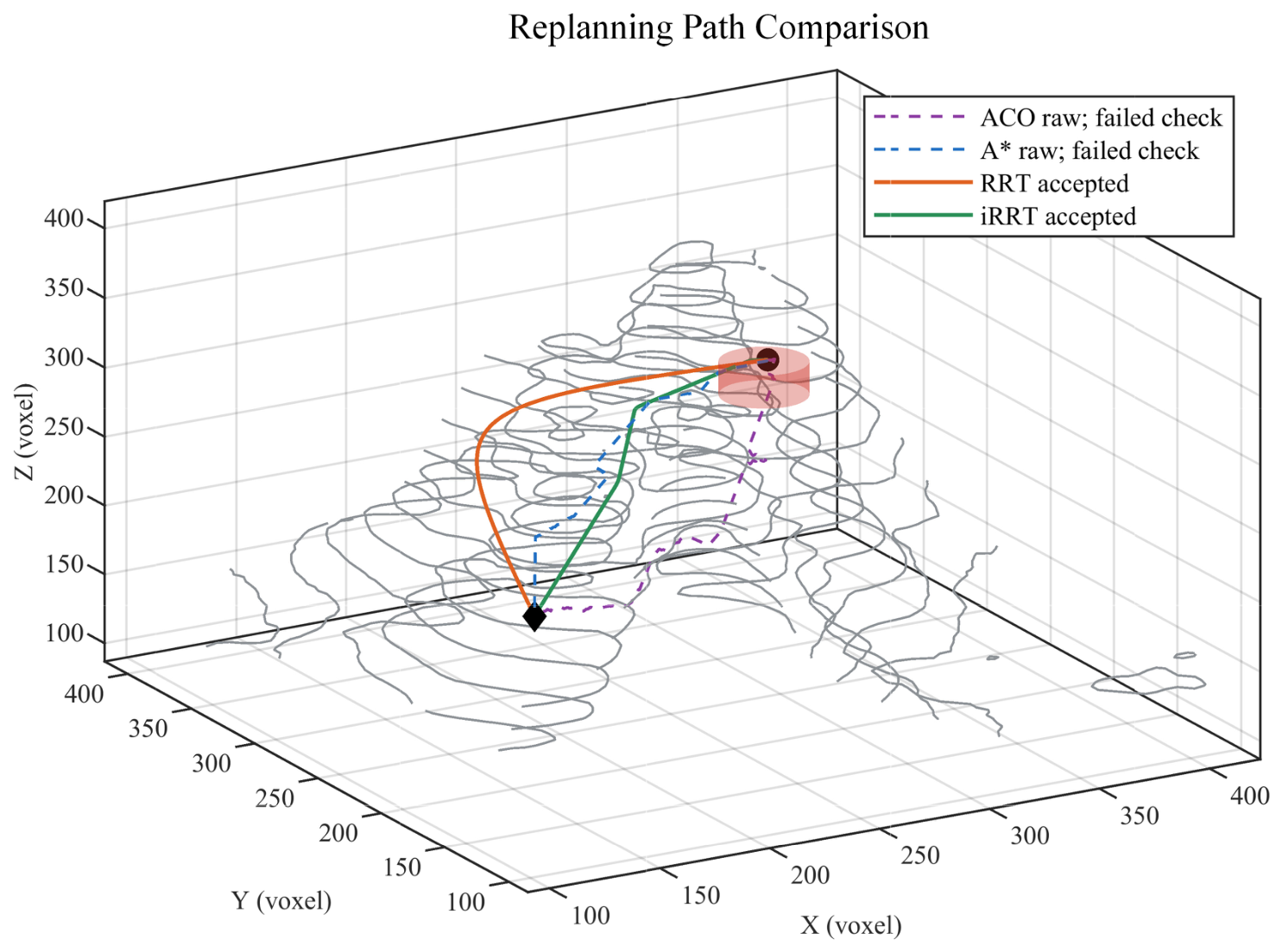
When a newly introduced fixed cylinder blocks the original route, the four planners are restarted from the same valid location. Their seed-1 responses are shown in the original four-panel order in Figure 10: A*, ACO, RRT, and iRRT. The A* and ACO raw routes show how these algorithms responded geometrically to the changed map, but they failed the additional common radius-two test and are drawn as dashed diagnostic paths. RRT and iRRT returned accepted detours around the new obstacle. Figure 11 overlays the same four responses to compare their route shapes before the quantitative summary in Table 2.

Figure 10. Seed-1 replanning responses after insertion of a fixed cylindrical obstacle: (a) A*, (b) ACO, (c) RRT, and (d) iRRT. Dashed routes in (a,b) are raw outputs that failed the additional common radius-two voxel-neighborhood test; solid routes in (c,d) are accepted, collision-checked paths.

Figure 11. Overall seed-1 comparison of four replanning routes on the updated voxel map. Solid RRT and iRRT routes passed the common test and postprocessing; dashed A* and ACO routes are shown as raw geometric responses only. Thirty-run safety and length measures are reported in Table 2.

In the representative replanning run, RRT and iRRT form accepted detours around the inserted cylinder. The A* and ACO raw routes are retained in Figure 10 and Figure 11 to show their geometric responses, but are drawn with dashed lines because they fail the additional common radius-two test. Figure 10 allows the local detour of each algorithm to be inspected separately. Figure 11 places the same four routes on the updated map for an overall geometric comparison; the thirty-run safety and length statistics are given in Table 2. No safe-path length is assigned to a dashed, unaccepted output.

Table 2 summarizes the thirty-run fixed-obstacle replanning results. All four methods returned a nonempty raw route, but only RRT and iRRT passed the additional common radius-two test in all 30 runs; ACO and A* each passed in 0/30 runs. Among safe routes, iRRT had a mean length of 295.52 ± 17.56 voxels, compared with 297.74 ± 22.08 voxels for RRT, an observed difference of 0.7%. The paired iRRT-minus-RRT length difference was −2.21 voxels, with a 95% seed-bootstrap interval of −10.46 to 6.22 voxels; hence, the length difference is not conclusive. Relative to RRT, iRRT used 12.8% fewer raw path nodes (52.3 versus 60.0) and 6.5% fewer expanded tree nodes (504 versus 539), whereas its mean planner time was slightly longer (0.030 versus 0.025 s) and its mean maximum turning angle was higher (14.8° versus 13.0°). The iRRT B-spline passed the post-smoothing collision check in 29/30 runs; the remaining run retained the collision-checked pruned path. These results support the replanning method’s safety and compactness under this test, without implying superiority in every metric.

To examine why the observed differences occur, a matched-budget component ablation was conducted separately from that in Table 1 and Table 2 (Supplementary Table S3). It showed no consistent stand-alone path-length gain from post-solution informed sampling, whereas checked shortcut pruning produced the largest change in the tested sequence. Additional sparse, dense, narrow-passage, and seabed maps were used to test the integrated pipeline (Supplementary Table S4 and Figure S1). Event-handoff policies and a continuously moving obstacle were also assessed in separate controlled experiments (Supplementary Table S5 and Figures S2 and S3). These experiments broaden the conditions examined but are not pooled with the original-map four-planner results.

4.2. Trajectory-Tracking Control Simulation

The static and replanned iRRT paths were used as reference trajectories to evaluate PID, MPC, MPC–PID, and MPC–PID with residual disturbance estimation (MPC–PID–DE). For each seed, the four controllers shared the same path reference and seeded wave phases. RMSE measures overall position error, maximum error captures the largest sampled deviation, mean error is the average over the complete run, terminal error is the final sampled deviation, and steady-state error is the mean over the final 5 s of the terminal hold. Tracking coordinates use the simulation conversion of 0.1 m/voxel, so all five errors are reported in meters.

Table 3 compares the four controller configurations on the same static iRRT reference path and matched wave phases. PID had the largest mean RMSE (0.1197 ± 0.0080 m). MPC reduced it to 0.0475 ± 0.0036 m, and adding PID correction to MPC gave 0.0463 ± 0.0035 m. With residual disturbance estimation, the full MPC–PID–DE configuration achieved 0.0407 ± 0.0048 m, a 12.1% reduction relative to MPC–PID and a 66.0% reduction relative to PID. Its mean, terminal, and final-hold errors were also lower than those of MPC–PID. The mean maximum errors of the two hybrid configurations were nearly identical (0.1778 versus 0.1775 m), indicating that the estimator primarily reduced accumulated and later error, rather than the largest sampled deviation. All four configurations completed the 30 matched numerical runs.

Table 3. Tracking-error comparison of four controllers for the static iRRT path. Values are mean ± sample SD across 30 matched seeds and are in meters. DE denotes residual disturbance estimation; steady-state error is averaged over the final 5 s of the terminal hold. All configurations completed 30/30 numerically stable runs under the stated attitude screening criterion; this count is not a mathematical closed-loop stability proof.

Controller	RMSE	Maximum Error	Mean Error	Terminal Error	Steady-State Error
PID	0.1197 ± 0.0080	0.3599 ± 0.0644	0.1056 ± 0.0048	0.0526 ± 0.0470	0.0620 ± 0.0257
MPC	0.0475 ± 0.0036	0.1796 ± 0.0319	0.0373 ± 0.0021	0.0302 ± 0.0205	0.0306 ± 0.0124
MPC–PID	0.0463 ± 0.0035	0.1775 ± 0.0317	0.0362 ± 0.0020	0.0299 ± 0.0202	0.0302 ± 0.0120
MPC–PID–DE	0.0407 ± 0.0048	0.1778 ± 0.0437	0.0310 ± 0.0022	0.0251 ± 0.0188	0.0247 ± 0.0095

The static results indicate an overall tracking benefit from disturbance estimation, but a replanned reference contains a sharper geometric transition. The next comparison therefore examines the same controllers after obstacle-triggered replanning.

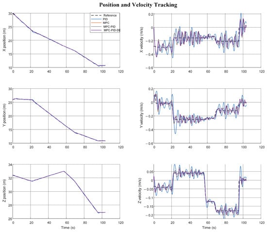
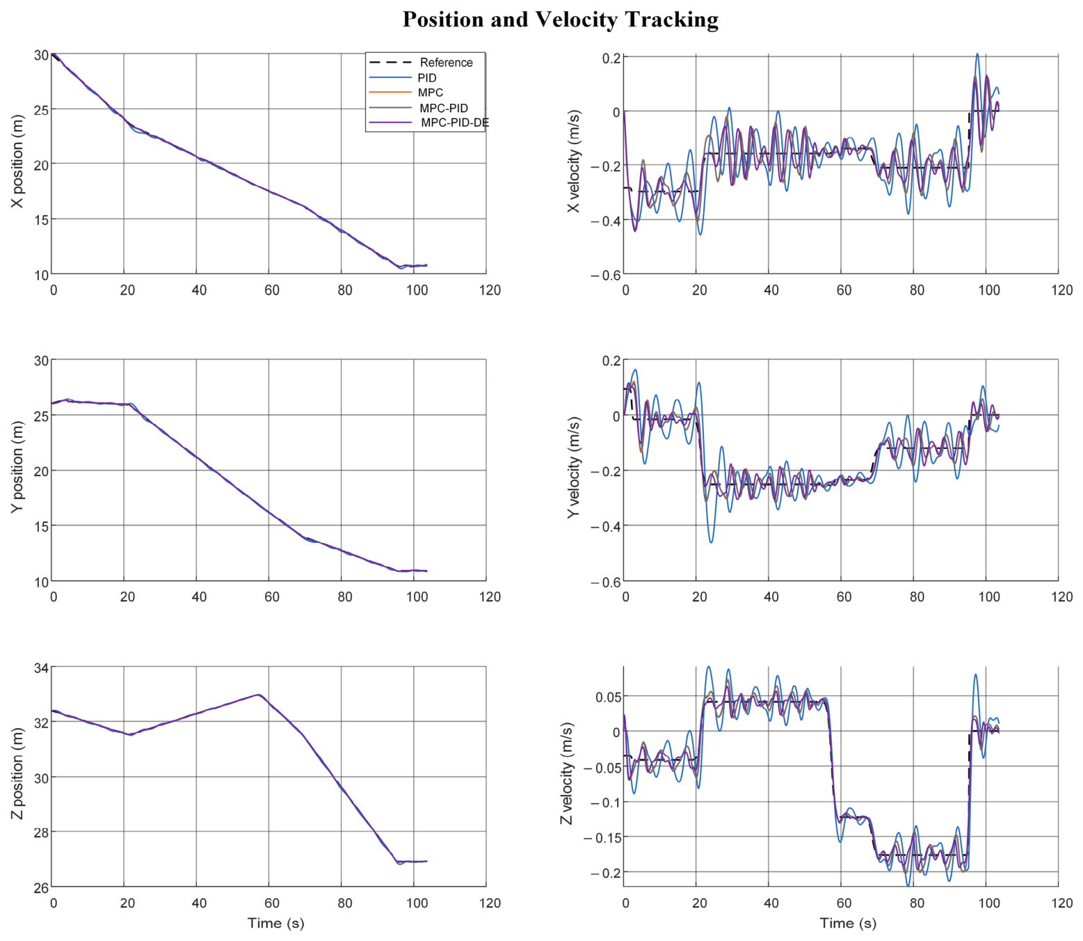
Figure 12 compares the translational position and velocity responses along the replanned iRRT reference in a representative seed-1 run. The position curves are close on the scale of the complete route, while the velocity panels make the local deviations around turns and depth changes easier to inspect. PID shows larger transient fluctuations; MPC and the two hybrid controllers remain closer to the common reference. A single trace illustrates the response shape, whereas Table 4 summarizes the 30 matched runs.

Figure 12. Translational position and inertial-frame velocity responses on the replanned iRRT path for PID, MPC, MPC–PID, and MPC–PID–DE in seed 1. The left panels show x, y, and z positions, and the right panels show the corresponding velocities; Table 4 gives 30-run tracking-error statistics.

Table 4. Tracking-error comparison of four controllers for the replanned iRRT path. Values are mean ± sample SD across 30 matched seeds and are in meters. The five error definitions and DE abbreviation follow Table 3. All configurations completed 30/30 numerically stable runs; the event-planning interval is excluded from controller-update timing.

Controller	RMSE	Maximum Error	Mean Error	Terminal Error	Steady-State Error
PID	0.1364 ± 0.0179	0.4152 ± 0.0963	0.1156 ± 0.0100	0.0974 ± 0.0573	0.0847 ± 0.0338
MPC	0.0552 ± 0.0107	0.1935 ± 0.0806	0.0426 ± 0.0050	0.0486 ± 0.0291	0.0429 ± 0.0157
MPC–PID	0.0535 ± 0.0097	0.1886 ± 0.0746	0.0414 ± 0.0047	0.0478 ± 0.0285	0.0421 ± 0.0152
MPC–PID–DE	0.0483 ± 0.0122	0.1889 ± 0.0873	0.0361 ± 0.0048	0.0301 ± 0.0237	0.0309 ± 0.0113

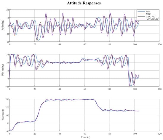
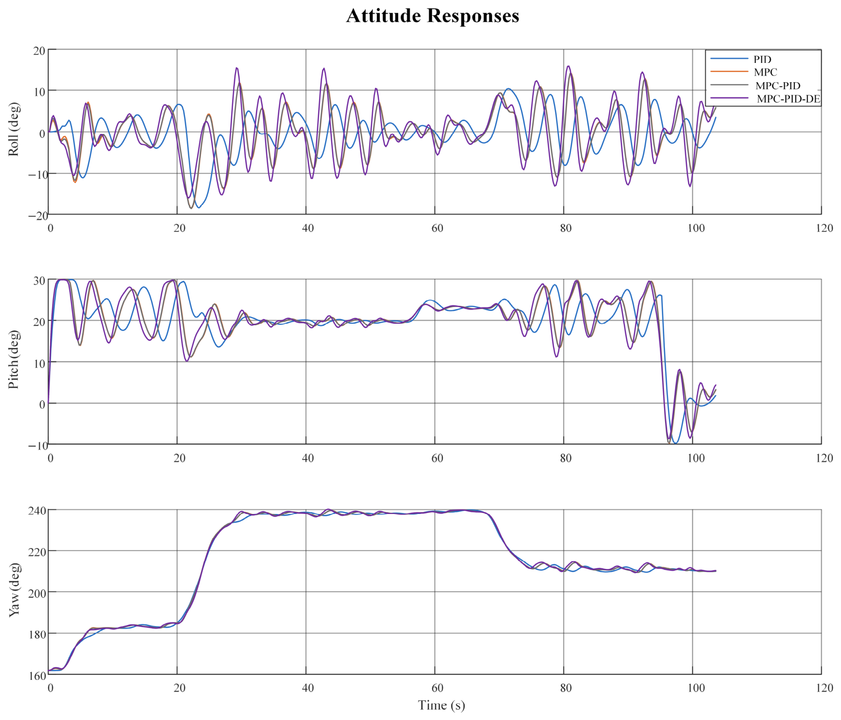
The attitude responses in Figure 13 show how the same controllers follow the orientation generated from the replanned trajectory. Their local deviations occur around the route transitions, so the curves are interpreted together with the position-error measures rather than as a separate proof of controller superiority.

Figure 13. Seed-1 roll, pitch, and yaw responses of PID, MPC, MPC–PID, and MPC–PID–DE on the replanned iRRT path. Angles are reported in degrees.

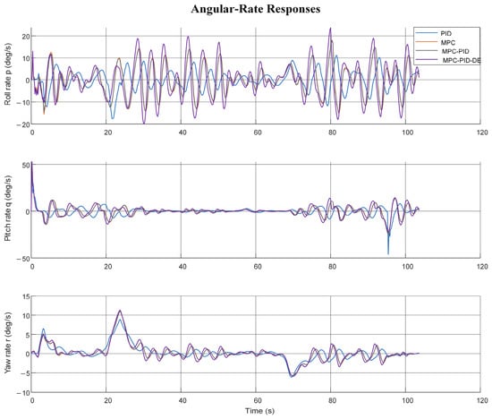
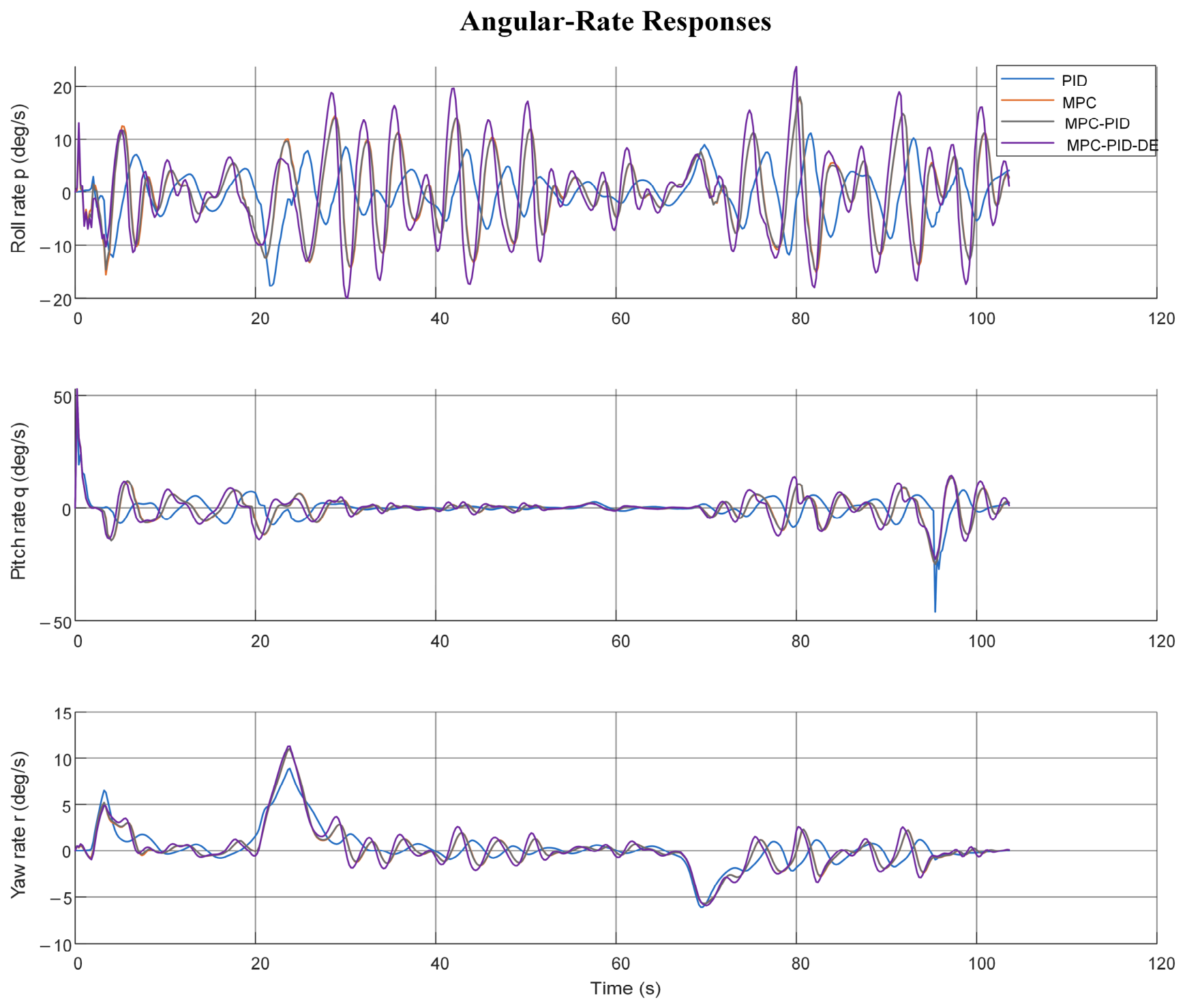
Figure 14 presents the corresponding body angular rates. The rate responses clarify the transient control effort underlying the attitude changes in Figure 13; all four curves use the same replanned path and wave realization.

Figure 14. Seed-1 body roll-, pitch-, and yaw-rate responses of the four controller configurations on the replanned iRRT path. Rates are reported in degrees per second.

Table 4 presents the corresponding results on the replanned iRRT path. PID again had the largest mean RMSE (0.1364 ± 0.0179 m), whereas MPC and MPC–PID gave 0.0552 ± 0.0107 and 0.0535 ± 0.0097 m, respectively. The full MPC–PID–DE controller achieved 0.0483 ± 0.0122 m, a 9.7% reduction relative to MPC–PID and a 64.6% reduction relative to PID. Its mean, terminal, and final-hold errors were also lower than those of MPC–PID. However, their mean maximum errors were nearly unchanged (0.1889 versus 0.1886 m). Each controller used the same reference path and wave phases within a seed, so the observed differences are attributable to the controller configuration under these numerical conditions rather than to different nominal routes.

The prescribed wave-proxy acceleration and its residual estimate are compared for the illustrative run in Supplementary Figure S4. The estimate follows the main disturbance trend with some delay, which is consistent with the lower mean tracking errors in Table 3 and Table 4 but does not by itself identify a physical wave-load model. For the complete controller, the mean MATLAB update duration was approximately 0.125 ms on the static path and 0.127 ms on the replanned path; the respective observed maxima were 1.801 and 0.588 ms. None of these recorded controller updates exceeded the 0.2 s simulation period. Timing excludes plotting and event replanning and therefore does not establish a hardware real-time guarantee.

4.3. Discussion

The results identify different contributions rather than a single best-performing algorithm. On the original map, the proposed iRRT configuration produced more compact tree paths than conventional RRT, but A* had the shortest accepted static path, and the paired RRT–iRRT path-length intervals included zero. In the matched-budget component sequence (Supplementary Table S3), collision-checked reverse greedy pruning produced the largest reduction in mean safe-path length. Optional post-solution informed sampling did not show a consistent independent gain within the evaluated computational budget. After the fixed-obstacle event, the checked B-spline failed in one of 30 iRRT runs, so the safe pruned path was retained. These observations explain both the benefit of the refinement pipeline and the need for a post-smoothing safety check and fallback.

Supplementary Table S5 also clarifies when guarded handoff is useful. In the 180 held-out paired cases, direct replanning and guarded short-prefix handoff both yielded 180/180 safe completed trajectories. The guarded policy reused a checked prefix only when the connection satisfied the turn and clearance guards; 61/180 candidates fell back to direct replanning. Compared with direct replanning, its mean maximum tracking error over the first 5 s was 0.1429 versus 0.1490 m, while mean planning-and-checking time increased from 0.249 to 0.339 s. Guarded handoff is therefore a conditional option when a checked prefix can be connected, and the extra computation is acceptable. Direct replanning remains appropriate when the candidate fails its checks, or lower latency is preferred. These cases do not establish a general safety advantage over direct replanning.

Recent underwater RRT studies have considered reinforcement-learning-guided dual-tree search [20] and RRT*-based cost-valley adaptive sampling [21]. The present work addresses a different coupled question: whether a radius-aware replanning handoff and checked path refinement can be connected to downstream six-degree-of-freedom tracking under matched references and disturbances. The methods in [20,21] were not reimplemented on the present maps; therefore, no cross-paper numerical ranking is claimed. The present ablation and common postprocessing comparison isolate the contributions that could be tested under one implementation, while a head-to-head comparison with recently published variants remains future work.

The numerical scope also limits interpretation. The additional radius-two check is a shared evaluation rule, not proof that ACO, A*, RRT, and iRRT used identical internal collision policies; in particular, a nonempty ACO or A* route that failed this extra check should not be described as a failure to return a path. The wave input is a reproducible TMA-shaped acceleration proxy without speed-dependent encounter frequencies or an identified wave-load transfer function. Full-state noiseless feedback, nominal model parameters, and a prescribed obstacle event were assumed. Although recorded MATLAB controller updates were below the 0.2 s simulation period, event replanning was excluded, and no onboard or experimental real-time guarantee follows. Pool or field measurements and a common implementation of newer RRT variants are needed to assess generality.

5. Conclusions

This study investigated path planning, obstacle-triggered replanning, and trajectory tracking for an underwater quadrotor vehicle in a three-dimensional nearshore environment. The enhanced RRT configuration combines guided search and locally adaptive extension with collision-checked reverse greedy pruning and B-spline smoothing. When a newly introduced obstacle blocks the remaining path, a radius-aware test and bisection-based handoff support local replanning. Post-solution informed sampling was assessed as a separate ablation rather than included in every four-planner comparison. For tracking, a translational MPC command is combined with weighted PID correction and residual disturbance estimation in a nonlinear six-degree-of-freedom simulation.

In 30 runs on the original static map, RRT and iRRT each produced 30/30 safe paths under the additional common radius-two test, whereas A* gave the shortest mean safe path. Relative to RRT, iRRT used 37.4% fewer raw path nodes and 33.1% fewer expanded tree nodes; its 1.7% lower mean path length did not establish a conclusive length advantage. After insertion of a fixed obstacle, RRT and iRRT again passed the common test in 30/30 runs. The iRRT route used 12.8% fewer raw nodes and 6.5% fewer expanded nodes than RRT, while the small mean length difference was inconclusive. In the matched six-degree-of-freedom tracking comparisons, adding residual disturbance estimation to MPC–PID reduced mean position RMSE by 12.1% on the static path and 9.7% on the replanned path, although the mean maximum error changed little. These findings demonstrate the contribution of the integrated modules within the tested numerical scenarios without asserting superiority in every planning or control metric.

The present study remains limited to numerical simulations with prescribed obstacle events, full-state feedback, a wave-shaped disturbance proxy, and model parameters that were not identified from a physical vehicle. The common radius-two test is an additional evaluation rule and does not by itself establish equivalent internal collision policies for the four planners. Future work will examine measured hydrodynamic disturbances, uncertain obstacle motion, onboard computation, and pool or field experiments to assess whether the observed planning and tracking benefits persist in a physical system.

References

- Sun, L.; Wang, Y.; Hui, X.; Ma, X.; Bai, X.; Tan, M. Underwater Robots and Key Technologies for Operation Control. Cyborg Bionic Syst. 2024, 5, 0089. [Google Scholar] [CrossRef] [Scilit] [PubMed]
- Nauert, F.; Kampmann, P. Inspection and Maintenance of Industrial Infrastructure with Autonomous Underwater Robots. Front. Robot. AI 2023, 10, 1240276. [Google Scholar] [CrossRef] [Scilit] [PubMed]
- Peck, C.J.; Langedock, K.; Boone, W.; Fourie, F.; Moulaert, I.; Semeraro, A.; Sterckx, T.; Geldhof, R.; Groenendaal, B.; Ponsoni, L. The Use of Autonomous Underwater Vehicles for Monitoring Aquaculture Setups in a High-Energy Shallow Water Environment: Case Study Belgian North Sea. Front. Mar. Sci. 2024, 11, 1386267. [Google Scholar] [CrossRef] [Scilit]
- Panda, M.; Das, B.; Subudhi, B.; Pati, B.B. A Comprehensive Review of Path Planning Algorithms for Autonomous Underwater Vehicles. Int. J. Autom. Comput. 2020, 17, 321–352. [Google Scholar] [CrossRef] [Scilit]
- Mohanty, P.K.; Chaudhary, V.; Prajapati, R. Review on Path Planning Methods for Autonomous Underwater Vehicle. Proc. Inst. Mech. Eng. Part M J. Eng. Marit. Environ. 2025, 239, 3–37. [Google Scholar] [CrossRef] [Scilit]
- Chen, Z.; Yan, J.; Huang, R.; Gao, Y.; Peng, X.; Yuan, W. Path Planning for Autonomous Underwater Vehicles (AUVs) Considering the Influences and Constraints of Ocean Currents. Drones 2024, 8, 348. [Google Scholar] [CrossRef] [Scilit]
- Garcia, D.G.; Medina, Y.V.; Hernández, L.; Martínez, A.; Espinosa, Y.M. Wave Disturbance Compensation for AUV Diving Control in Shallow Water Environment. J. Appl. Res. Technol. 2019, 17, 326–337. [Google Scholar] [CrossRef] [Scilit]
- Wang, C.; Yu, W.; Zhu, S.; Song, L.; Guan, X. Safety-Critical Trajectory Generation and Tracking Control of Autonomous Underwater Vehicles. IEEE J. Ocean. Eng. 2023, 48, 93–111. [Google Scholar] [CrossRef] [Scilit]
- Hart, P.E.; Nilsson, N.J.; Raphael, B. A Formal Basis for the Heuristic Determination of Minimum Cost Paths. IEEE Trans. Syst. Sci. Cybern. 1968, 4, 100–107. [Google Scholar] [CrossRef] [Scilit]
- Lai, Y.; Shang, J.; Liu, Z.; Jiang, Z.; Li, Y.; Chen, L. Deep-Sea A*+: An Advanced Path Planning Method Integrating Enhanced A* and Dynamic Window Approach for Autonomous Underwater Vehicles. In Proceedings of the 2024 5th International Conference on Big Data, Artificial Intelligence and Internet of Things Engineering (ICBAIE), Shenzhen, China, 25–27 October 2024. [Google Scholar]
- Meng, R.; Sun, A.; Wu, Z.; Du, X.; Meng, Y. 3D Smooth Path Planning of AUV Based on Improved Ant Colony Optimization Considering Heading Switching Pressure. Sci. Rep. 2023, 13, 12348. [Google Scholar] [CrossRef] [Scilit] [PubMed]
- Yuan, X.; Wang, J.; Tong, C.; Wang, H. Integrated Path Planning for AUV Communication Efficiency and Obstacle Avoidance Based on Ant Colony Optimization and Three-Dimensional Dynamic Window Algorithm. Appl. Ocean Res. 2025, 156, 104465. [Google Scholar] [CrossRef] [Scilit]
- Gupta, S.; Kumar, A.; Kumar, V.; Singh, S.; Sachin; Gautam, M. Autonomous Underwater Vehicle Path Planning Using Fitness-Based Differential Evolution Algorithm. J. Comput. Sci. 2024, 85, 102498. [Google Scholar] [CrossRef] [Scilit]
- Tan, J.; Sun, Y.; Cai, K.; Zhang, Y.; Zhang, L. Energy-Efficient AUV Path Planning under Multiple Constraints Using a Synergistic Differential Evolution Algorithm. J. Mar. Sci. Appl. 2025. [Google Scholar] [CrossRef] [Scilit]
- Liu, S.; Wang, Z.; Wang, T.; Zhou, S.; Zhang, Y.; Jin, P.; Yang, G. Energy-Optimized Path Planning for Fully Actuated AUVs in Complex 3D Environments. J. Mar. Sci. Eng. 2025, 13, 1269. [Google Scholar] [CrossRef] [Scilit]
- Lavalle, S.M. Rapidly-Exploring Random Trees: A New Tool for Path Planning; Computer Science Department, Iowa State University: Ames, IA, USA, 1998. [Google Scholar]
- Kuffner, J.J.; LaValle, S.M. RRT-Connect: An Efficient Approach to Single-Query Path Planning. In Proceedings of the 2000 IEEE International Conference on Robotics and Automation; IEEE: New York, NY, USA, 2000; Volume 2, pp. 995–1001. [Google Scholar]
- Karaman, S.; Frazzoli, E. Sampling-Based Algorithms for Optimal Motion Planning. Int. J. Robot. Res. 2011, 30, 846–894. [Google Scholar] [CrossRef] [Scilit]
- Gammell, J.D.; Srinivasa, S.S.; Barfoot, T.D. Informed RRT*: Optimal Sampling-Based Path Planning Focused via Direct Sampling of an Admissible Ellipsoidal Heuristic. In Proceedings of the 2014 IEEE/RSJ International Conference on Intelligent Robots and Systems; IEEE: New York, NY, USA, 2014; pp. 2997–3004. [Google Scholar]
- Song, Y.; Chen, G.; Chen, Y.; Gao, J. Reinforcement Learning-Based Fast-Dual-Tree RRT Path Planning for Unmanned Underwater Vehicles. Ocean Eng. 2025, 342, 122937. [Google Scholar] [CrossRef] [Scilit]
- Ge, Y.; Eidsvik, J.; Olaisen, A.J.H. RRT*-Enhanced Long-Horizon Path Planning for AUV Adaptive Sampling Using a Cost Valley. Knowl.-Based Syst. 2025, 315, 113261. [Google Scholar] [CrossRef] [Scilit]
- He, L.; Xie, M.; Zhang, Y. A Review of Path Following, Trajectory Tracking, and Formation Control for Autonomous Underwater Vehicles. Drones 2025, 9, 286. [Google Scholar] [CrossRef] [Scilit]
- Liu, Y.; Zhang, H.; Zhang, X. Trajectory Tracking Control of Unmanned Underwater Vehicle Based on Projected Perpendicular Guidance Method with Disturbance Observer. J. Mar. Sci. Eng. 2024, 12, 901. [Google Scholar] [CrossRef] [Scilit]
- Yan, T.; Xu, Z.; Yang, S.X. Consensus Formation Tracking for Multiple AUV Systems Using Distributed Bioinspired Sliding Mode Control. IEEE Trans. Intell. Veh. 2023, 8, 1081–1092. [Google Scholar] [CrossRef] [Scilit]
- Deng, L.; Tao, J. Disturbance Observer Based Fractional-Order Sliding Mode Control for Underwater Vehicle with Variable Center of Mass. Meas. Control 2026, 59, 745–757. [Google Scholar] [CrossRef] [Scilit]
- Ma, C.; Tang, Y.; Lei, M.; Jiang, D.; Luo, W. Trajectory Tracking Control for Autonomous Underwater Vehicle with Disturbances and Input Saturation Based on Contraction Theory. Ocean Eng. 2022, 266, 112731. [Google Scholar] [CrossRef] [Scilit]
- Heshmati-alamdari, S.; Nikou, A.; Dimarogonas, D.V. Robust Trajectory Tracking Control for Underactuated Autonomous Underwater Vehicles. In Proceedings of the 2019 IEEE 58th Conference on Decision and Control (CDC); IEEE: New York, NY, USA, 2019; pp. 8311–8316. [Google Scholar]
- Dai, L.; Zhang, D.; Wang, S.; Nie, G.; Zhu, X.; Wang, X. Trajectory Tracking Control of an Autonomous Underwater Vehicle under Disturbance and Model Uncertainty. J. Mar. Sci. Eng. 2025, 13, 2210. [Google Scholar] [CrossRef] [Scilit]
- Zhu, Y.; Sun, B.; Liu, X. Event-Triggered Model Predictive Control for Trajectory Tracking of AUV with an Adaptive Disturbance Observer. In Proceedings of the 2024 10th International Conference on Systems and Informatics (ICSAI); IEEE: New York, NY, USA, 2024; pp. 1–6. [Google Scholar]
- Bao, H.; Zhu, H. Modeling and Trajectory Tracking Model Predictive Control Novel Method of AUV Based on CFD Data. Sensors 2022, 22, 4234. [Google Scholar] [CrossRef] [Scilit] [PubMed]
- Jimoh, I.A.; Yue, H. Path Following Model Predictive Control of a Coupled Autonomous Underwater Vehicle. IFAC-Pap. 2024, 58, 183–188. [Google Scholar] [CrossRef] [Scilit]
- Hu, Y.; Li, B.; Jiang, B.; Han, J.; Wen, C.-Y. Disturbance Observer-Based Model Predictive Control for an Unmanned Underwater Vehicle. J. Mar. Sci. Eng. 2024, 12, 94. [Google Scholar] [CrossRef] [Scilit]
- Gao, J.; Zhang, G.; Wu, P.; Zhao, X.; Wang, T.; Yan, W. Model Predictive Visual Servoing of Fully-Actuated Underwater Vehicles with a Sliding Mode Disturbance Observer. IEEE Access 2019, 7, 25516–25526. [Google Scholar] [CrossRef] [Scilit]
- Fu, H.; Yao, W.; Cajo, R.; Zhao, S. Trajectory Tracking Predictive Control for Unmanned Surface Vehicles with Improved Nonlinear Disturbance Observer. J. Mar. Sci. Eng. 2023, 11, 1874. [Google Scholar] [CrossRef] [Scilit]
- Kang, S.; Rong, Y.; Chou, W. Antidisturbance Control for AUV Trajectory Tracking Based on Fuzzy Adaptive Extended State Observer. Sensors 2020, 20, 7084. [Google Scholar] [CrossRef] [Scilit] [PubMed]
- Walker, K.L.; Giorgio-Serchi, F. Disturbance Preview for Nonlinear Model Predictive Trajectory Tracking of Underwater Vehicles in Wave Dominated Environments. In Proceedings of the 2023 IEEE/RSJ International Conference on Intelligent Robots and Systems (IROS), Detroit, MI, USA, 1–5 October 2023. [Google Scholar]
- Chen, Y.; Fei, X.; Mu, X.; Zhao, X.; Zhang, S.; Yang, C. Research on the Pitch Angle Attitude Control of Underwater Vehicles Based on a Novel Butterfly-Shaped Blocks Structure. Ocean Eng. 2024, 313, 119523. [Google Scholar] [CrossRef] [Scilit]
- Zhuo, J.; Tian, X.; Liu, H. Distributed Cooperative H∞ Optimal Control of Underactuated Autonomous Underwater Vehicles Based on Reinforcement Learning and Prescribed Performance. Ocean Eng. 2024, 312, 119323. [Google Scholar] [CrossRef] [Scilit]
- Wang, J.; Xiang, G.; Xiang, X.; Soares, C.G. A High Fidelity Simulation for Vertical Planar Motion Control of Underwater Vehicle Navigating near Surface Waves Using Joint Mechanism Control. Mech. Mach. Theory 2025, 212, 106056. [Google Scholar] [CrossRef] [Scilit]
- Xu, S.; Wu, J.; Zhang, S.; Yang, X. Hydrodynamic Analysis of a Tethered Underwater Robot with Control Equipment Subjected to Cnoidal Waves. Ocean Eng. 2022, 243, 110264. [Google Scholar] [CrossRef] [Scilit]
- Hasan, M.W.; Abbas, N.H. Disturbance Rejection for Underwater Robotic Vehicle Based on Adaptive Fuzzy with Nonlinear PID Controller. ISA Trans. 2022, 130, 360–376. [Google Scholar] [CrossRef] [Scilit] [PubMed]
- Chen, L.; Cui, R.; Yan, W.; Xu, H.; Zhao, H.; Li, H. Design and Climbing Control of an Underwater Robot for Ship Hull Cleaning. Ocean Eng. 2023, 274, 114024. [Google Scholar] [CrossRef] [Scilit]
Disclaimer/Publisher’s Note: The statements, opinions and data contained in all publications are solely those of the individual author(s) and contributor(s) and not of MDPI and/or the editor(s). MDPI and/or the editor(s) disclaim responsibility for any injury to people or property resulting from any ideas, methods, instructions or products referred to in the content. |
© 2026 by the authors. Licensee MDPI, Basel, Switzerland. This article is an open access article distributed under the terms and conditions of the Creative Commons Attribution (CC BY) license.