A Low-Power Ultrasonic Residual Stress Measurement Method Based on the CM-SSA-VMD Denoising Algorithm

Abstract

Welded structures are widely used in ships and marine equipment. The ultrasonic longitudinal critically refracted (LCR) wave method is a reliable technique for measuring residual stress in welded structures. Conventional ultrasonic measurement systems have high power consumption and are difficult to operate under the limited power supply conditions of marine environments. Reducing the excitation voltage can lower power consumption, but as the excitation voltage decreases, ultrasonic echo energy weakens and noise interference increases, thereby affecting the accuracy of stress measurement. This paper proposes a complexity-mutation-based adaptive singular spectrum analysis–variational mode decomposition algorithm (CM-SSA-VMD). The algorithm constructs a complexity index using the spectral centroid, waveform roughness, and zero-crossing rate. By identifying abrupt changes in complexity between adjacent singular spectrum analysis (SSA) components, it adaptively determines which components to retain for reconstruction. Then, variational mode decomposition (VMD) is used to further separate the residual high-frequency noise. Finally, the ultrasonic time of flight (TOF) is estimated using the cross-correlation algorithm, and the stress is calculated. The stress measurement accuracy of the proposed algorithm was evaluated at different excitation voltages: 5.2 V, 3.3 V, 1.2 V, and 0.5 V. The results show that when the excitation voltage drops to 0.5 V, after being processed by CM-SSA-VMD, the average relative error of stress measurement remains below 10%, while the average relative errors of a new adaptive denoising method, Grey Wolf Optimization–Variational Mode Decomposition–Wavelet Transform (GWO-VMD-WT), traditional FIR filtering and VMD are approximately 14%, 18% and 16% respectively. Compared with GWO-VMD-WT, FIR filtering and VMD, the measurement accuracy of this method is improved by 33.35%, 46.16% and 41.82% respectively. The CM-SSA-VMD algorithm can effectively suppress noise in ultrasonic signals at low excitation voltages and improve the reliability of stress monitoring. It provides a feasible method for low-power ultrasonic residual stress monitoring in marine engineering.

1. Introduction

Welded structures are widely used in ships and marine engineering, and their quality directly affects structural integrity [1]. During hull construction, longitudinal stiffeners, ribs, and shell plates are welded together to form numerous stiffened plate structures, resulting in biaxial residual stresses in the welded regions [2]. Under long-term service conditions, the superposition of residual stress, wave-induced cyclic loading, and working stress can reduce the ultimate load-carrying capacity of stiffened structures [3]. Therefore, residual stress detection in critical welded regions of ships is of great significance for evaluating welding quality and ensuring structural safety and reliability.

The primary methods for residual stress measurement include the hole-drilling method [4], X-ray diffraction method [5], Electromagnetic ultrasonic method [6], and ultrasonic method [7,8]. The hole-drilling method releases local stress by drilling a small hole in the material surface and calculates the pre-existing residual stress based on the strain-release principle. This method is portable and relatively inexpensive [9]; however, it damages the integrity of welded components [10]. Therefore, it is mainly used for laboratory testing and has inherent limitations in field applications. The X-ray diffraction method determines residual stress by measuring changes in lattice spacing and offers the advantages of being nondestructive and providing high measurement accuracy at the material surface [5]. However, the required equipment is relatively expensive, and strict radiation protection measures must be implemented during measurement. In field inspections of welded components, its application is therefore constrained by equipment deployment and radiation safety requirements. Although the electromagnetic ultrasonic method is convenient to operate and does not damage the components, its accuracy is relatively low [11]. The ultrasonic method is based on the acoustoelastic effect, evaluating residual stress by measuring changes in ultrasonic propagation time caused by stress variations. It has the advantages of being nondestructive, portable, and highly efficient [12], and has been widely used for residual stress measurement in welded components.

For the ultrasonic equipment installed on ships and used for long-term monitoring, replacing the batteries is quite difficult, thus limiting the working time of the equipment to a certain extent. In order to ensure that the equipment can operate for a long time, its power consumption is usually reduced to increase the working time [13]. Xiao et al. [14] achieved ultrasonic monitoring with a power consumption of 0.83 mW using a 10 V excitation voltage. Marcus et al. [15] achieved ultrasonic monitoring with a power consumption of 1.5 mW using a 5 V excitation voltage. These studies show that reducing the ultrasonic excitation voltage can effectively lower equipment power consumption. However, a lower excitation voltage reduces the energy of the received signal and increases noise interference [16]. Therefore, effectively suppressing signal noise is the key to achieving low-voltage and low-power ultrasonic stress monitoring.

Existing signal denoising algorithms include wavelet thresholding [17], Empirical Mode Decomposition (EMD) [18], and Variational Mode Decomposition (VMD) [19]. Wavelet thresholding decomposes ultrasonic signals into different frequency bands through multiscale analysis. Subsequently, the wavelet coefficients of the high-frequency signals are thresholded to suppress high-frequency noise and reconstruct the waveform. However, this algorithm requires manual selection of the wavelet basis, decomposition level, and thresholding function, which greatly limits its performance in practical applications [20,21]. EMD provides adaptive mode decomposition without requiring preset parameters, and is suitable for processing nonstationary signals. Therefore, it has been widely used for signal denoising [22,23,24]. However, EMD may produce spurious components and mode mixing. To solve these problems, Wu et al. [25] proposed the Ensemble Empirical Mode Decomposition (EEMD). This algorithm alleviates mode mixing by adding a finite amount of white noise to the signal. However, it requires repeated EMD decompositions and ensemble averaging, resulting in higher computational cost. In addition, the added white noise is difficult to completely remove during signal reconstruction. The VMD algorithm improves upon EMD and EEMD. By solving a constrained variational problem, it can adaptively determine the finite bandwidth and optimal center frequency of each mode, effectively separating each mode component. This algorithm not only improves signal decomposition efficiency but also effectively avoids mode mixing [19].

At present, some researchers have combined different denoising algorithms to improve denoising performance. Yang et al. [26] proposed a combined denoising algorithm based on CEEMDAN and wavelet packet thresholding. CEEMDAN was used to reduce reconstruction error, and wavelet packet thresholding was then employed to restore and retain the high-frequency effective components. Compared with EEMD, this algorithm improved the Signal-to-Noise Ratio (SNR) of the reconstructed signal by 48.03%. However, it still requires manual parameter selection and has limited generalization ability. He et al. [27] combined EMD with wavelet packet transform and used different wavelet basis functions for different EMD components, effectively suppressing noise interference. However, when a signal contains components with large frequency differences but similar amplitudes, EMD decomposition is still prone to mode mixing [28].

To solve the above problems, this paper proposes a complexity-mutation-based adaptive Singular Spectrum Analysis–Variational Mode Decomposition (CM-SSA-VMD) denoising algorithm. This algorithm constructs the complexity index by using spectral center, waveform roughness, and zero-crossing rate. The components retained for SSA reconstruction are adaptively determined based on abrupt changes in complexity. Subsequently, the VMD algorithm is employed to further denoise the retained components, suppressing high-frequency noise, in order to obtain the final denoised signal. To evaluate the algorithm performance, the CM-SSA-VMD algorithm was compared with the GWO-VMD-WT algorithm, VMD algorithm and the FIR filter at initial SNRs of 0, 2, 5, 10, and 15 dB. The results showed that the average SNR increment of the CM-SSA-VMD algorithm under different initial SNRs was over 12 dB, and the Root Mean Square Error (RMSE) was lower than 0.1. The average SNR improvements of the GWO-VMD-WT, the VMD and the FIR algorithms were approximately 3.1 dB, 4.5 dB and 3.4 dB lower than that of the CM-SSA-VMD algorithm, respectively.

To verify the effectiveness of the CM-SSA-VMD algorithm, stress measurement accuracy tests were conducted on 7-series aluminum alloy plates under low excitation voltages of 5.2 V, 3.3 V, 1.2 V, and 0.5 V. The results showed that when the excitation voltage decreased from 5.2 V to 0.5 V, the average relative error of CM-SSA-VMD remained within 10%, while the average relative error of GWO-VMD-WT was above 10% at 3.3 V. Moreover, the effects of VMD and FIR were worse than those of GWO-VMD-WT, with the average relative error being above 10% below 5.2 V. The overall measurement accuracy of CM-SSA-VMD was superior to those of GWO-VMD-WT, VMD, and FIR methods. During the experiment, the power consumption of the equipment was also measured. The results indicated that as the excitation voltage decreased, the power consumption gradually decreased. When the excitation voltage was as low as 0.5 V, the power consumption was approximately 13 mW. This verified the feasibility of the CM-SSA-VMD method for stress measurement under low excitation voltages.

To further verify the applicability of the CM-SSA-VMD method, residual stress measurements were conducted on the aluminum alloy plates subjected to MIG welding at low excitation voltages of 5.2 V, 3.3 V, 1.2 V, and 0.5 V. At a low excitation voltage of 0.5 V, the stress measurement accuracy was verified for six materials: 5083-H116 aluminum alloy, 6061-T6 aluminum alloy, 316L austenitic stainless steel, 2205 duplex stainless steel, Q235 carbon structural steel, and AH36 high-strength shipbuilding steel. The welding residual stress measurement experiments demonstrated that the test results at low voltages were consistent with the reference results in terms of the residual stress trend, and the average relative errors at the four low excitation voltages were all below 10%. The results indicated that for aluminum alloy plates subjected to MIG welding, the CM-SSA-VMD method can detect the residual stress of the welding structure using low excitation voltages. The precision verification experiments for different materials showed that the average relative errors for the six materials were all below 10%. This indicates that the CM-SSA-VMD method has certain applicability for the above materials under low voltage excitation conditions.

It should be noted that steel is currently the main material for large ships. However, for ships with high speed requirements and the need for lightweight structures, marine-grade 5-series and 6-series aluminum alloys are typically used for structural components such as hull plates, decks, and reinforcing ribs [29,30]. Compared with the aluminum alloys of the 5th and 6th series, the 7th series aluminum alloy has a stronger load-bearing capacity and has certain research value for ships with high requirements for high strength. Therefore, in this paper, 7th series aluminum alloy sheets are used to verify the effectiveness of the CM-SSA-VMD method under laboratory conditions. It is important to note that the selection of 7-series aluminum alloy sheet was not because it better represents the ship structure than steel, but rather as a high-strength aluminum alloy sample. The main focus is on the accuracy of the CM-SSA-VMD method in measuring stress under low excitation voltage.

2. Measurement Theory

2.1. Theory of Residual Stress Measurement Based on LCR Waves

The acoustoelastic effect provides the theoretical basis for residual stress measurement using LCR waves. According to the acoustoelastic effect, when a material is subjected to stress, LCR wave velocity and time of flight (TOF) will change. For an isotropic medium, the relationship between LCR wave velocity and stress is expressed as:

$$\rho V^2=\lambda +2\mu +{\displaystyle \frac{\sigma }{3\lambda +2\mu }}\left[{\displaystyle \frac{\lambda +\mu }{\mu }}\left(4\lambda +10\mu +4m\right)+\lambda +2l\right]$$

(1)

where $V$ is the wave velocity, $\sigma$ is the stress, $\rho$ is the material density, $\lambda$ and $\mu$ are the second-order elastic constants of the material, and $l$ and $m$ are the third-order elastic constants of the material.

According to Equation (1), when the specimen is in a stress-free state, the wave velocity is:

$$V_0=\sqrt{{\displaystyle \frac{\lambda +2\mu }{\rho }}}$$

(2)

where $V_0$ is the wave velocity in the stress-free state.

Combining Equations (1) and (2), and obtain:

$$V=V_0\sqrt{\left(1+k\mathsf{\sigma }\right)}$$

(3)

where $k={\displaystyle \frac{\frac{\lambda +\mu }{\mu }\left(4\lambda +10\mu +4m\right)+\lambda +2l}{\left(3\lambda +2\mu \right)\left(\lambda +2\mu \right)}}$ is the acoustoelastic coefficient.

Because the change in wave velocity caused by residual stress is relatively small, assuming that $\left|k\sigma \right|\ll 1$ is satisfied, we perform a first-order Taylor expansion on $\sqrt{\left(1+k\mathsf{\sigma }\right)}$:

$$V\approx V_0\left(1+{\displaystyle \frac{k}{2}}\mathsf{\sigma }\right)$$

(4)

Assuming that the LCR wave propagation distance is $L$, and $t$($t={\displaystyle \frac{L}{V}}$) and $t_0$($t_0={\displaystyle \frac{L}{V_0}}$) are the propagation times in the stressed and stress-free states, substituting them into Equation (4) gives:

$$\sigma \approx {\displaystyle \frac{-2}{k{t}_0}}\left(t-t_0\right)$$

(5)

Let $K={\displaystyle \frac{-2}{k{t}_0}}$ denote the calibration coefficient and $\Delta t=\left(t-t_0\right)$ the time of flight difference. Substituting them into Equation (5) gives:

$$\sigma =K\Delta t$$

(6)

The above equation is used to calculate residual stress and shows that the residual stress is linearly related to TOF difference.

2.2. Singular Spectrum Analysis

Singular spectrum analysis (SSA) is a signal processing algorithm based on subspace decomposition that can be used to denoise time series signals. The core idea of SSA is to perform singular value decomposition on the trajectory matrix to obtain different components and retain the components that can represent the clean signal to reconstruct the signal. The traditional SSA denoising steps are as follows:

Step 1: Convert the original data into a trajectory matrix

Assuming the original time-series signal of length $N$ is discretely represented as:

$$x(n)={[x_1,x_2,\dots ,x_N]}^T$$

(7)

Determine the window length $L$ (which must satisfy $2\le L\le N-1$) and the number of matrix columns $K$($K=N-L+1$), and construct the trajectory matrix $X$ based on $L$ and $K$:

$$X=\left[\begin{array}{ccccc}{x}_1& x_2& x_3& \cdots & x_K\\ x_2& x_3& x_4& \cdots & x_{K+1}\\ x_3& x_4& x_5& \cdots & x_{K+2}\\ ⋮& ⋮& ⋮& \ddots & ⋮\\ x_L& x_{L+1}& x_{L+2}& \cdots & x_N\end{array}\right]$$

(8)

where the matrix size is $L\times K$, and each column is a continuous discrete signal of length $L$. The next column is shifted one discrete signal point backward relative to the previous column.

Step 2: Singular value decomposition

Construct the covariance matrix $S$ of matrix $X$ and perform eigenvalue decomposition:

$$S=X{X}^T$$

(9)

$$S{u}_i={\lambda }_i{u}_i,\hspace{1em}\hspace{1em}i=1,2,\dots ,d$$

(10)

where $d$ is the rank of matrix $X$, ${\lambda }_i$ is the $i$th non-zero eigenvalue, and $u_i$ is the $i$th left singular vector.

Based on the eigenvalues and left singular vectors, calculate the singular values and right singular vectors of matrix $X$:

$${\sigma }_i=\sqrt{{\lambda }_i},\hspace{1em}\hspace{1em}i=1,2,\dots ,d$$

(11)

$$v_i={\displaystyle \frac{X^T{u}_i}{{\sigma }_i}},\hspace{1em}\hspace{1em}i=1,2,\dots ,d$$

(12)

where ${\sigma }_i$ is the $i$th singular value, and $v_i$ is the $i$th right singular vector.

The singular values and the left and right singular vectors are assembled into matrices $\Sigma$($\Sigma =diag\left({\sigma }_1,{\sigma }_2,\dots ,{\sigma }_d\right)$), $U$($U=\left[u_1,u_2,\dots ,u_d\right]$) and $V$($V=\left[v_1,v_2,\dots ,v_d\right]$), respectively. Matrix $X$ can be further expressed as:

$$X=U\Sigma V^T={\displaystyle {\displaystyle \sum }_{i=1}^d}{\sigma }_i{u}_i{v}_i^T$$

(13)

where ${\sigma }_i{u}_i{v}_i^T$ is the $i$th SSA component, and ${\sigma }_i$ reflects the energy contribution of the $i$th component in matrix $X$. In general, components associated with larger ${\sigma }_i$ values contain the main structure of the original signal, whereas those associated with smaller ${\sigma }_i$ values are generally regarded as noise.

Step 3: Signal reconstruction

The matrix obtained after reconstructing the components is:

$$X_s={\displaystyle \sum }_{i\in I_s}{\sigma }_i{u}_i{v}_i^T$$

(14)

where $I_s$ is the index set of the components retained for reconstruction.

Calculate the average value of the diagonal of matrix $X_s$, and restore the two-dimensional matrix into a one-dimensional discrete signal

$${\widehat{x}}_n={\displaystyle \frac{1}{W_n}}{\displaystyle \sum }_{\begin{array}{c}i+j=n+1\end{array}}{x}_{ij}^s,\hspace{1em}\hspace{1em}n=1,2,\dots ,N$$

(15)

$$\widehat{x}=\left[{\widehat{x}}_1,{\widehat{x}}_2,\dots ,{\widehat{x}}_N\right]$$

(16)

where ${\widehat{x}}_n$ is the $n$th reconstructed discrete signal, $W_n$ is the number of elements on the $n$th sub-diagonal, $x_{ij}^s$ is the element in the $i$th row and $j$th column of matrix $X_s$, and $\widehat{x}$ is the final one-dimensional discrete signal.

2.3. Variational Mode Decomposition

The core idea of VMD denoising is to use variational optimization and frequency-domain analysis to decompose the original signal into several narrowband components with different central frequencies, and reconstruct the signal using appropriate components [26,27]. The traditional VMD denoising process is as follows:

Step 1: Setting the parameters

Determine the main parameters of the VMD algorithm, including the number of modes $K$, penalty factor $\alpha$, and convergence threshold $\epsilon$.

Step 2: Constructing analytical signals and frequency shifting

To calculate the center frequency and bandwidth of each component in the positive frequency range, the Hilbert transform is applied to each component to construct its analytic signal:

$$u_k^{+}\left(t\right)=\left(\delta \left(t\right)+{\displaystyle \frac{j}{\pi t}}\right)\ast u_k\left(t\right),\hspace{1em}k=1,2,\dots ,K$$

(17)

where $u_k^{+}\left(t\right)$ is the analytic signal corresponding to the $k$th component, $\delta \left(t\right)$ is the Dirac unit impulse function, $j$ is the imaginary unit (satisfying $j^2=-1$), ${\displaystyle \frac{1}{\pi t}}$ is the convolution kernel of the Hilbert transform, and $u_k\left(t\right)$ is the $k$th component.

To accurately calculate the bandwidth of each component, the frequency shifting is then applied to the signal:

$$v_k\left(t\right)=u_k^{+}\left(t\right)e^{-j{\omega }_{k}t}$$

(18)

where ${\omega }_k$ is the center angular frequency of the $k$th component.

Step 3: Formulating the constrained variational model

Under the constraints of ${\displaystyle {\displaystyle \sum }_{k=1}^K}{u}_k\left(t\right)=f\left(t\right)$, a variational model is formulated by minimizing the sum of the bandwidths of all components:

$$\underset{\left\{u_k\right\},\left\{{\omega }_k\right\}}{\min }{\displaystyle {\displaystyle \sum }_{k=1}^K}\parallel {\partial }_t{v}_k\left(t\right){\parallel }_2^2$$

(19)

where $\left\{u_k\right\}=\left\{u_1\left(t\right),u_2\left(t\right),\dots ,u_K\left(t\right)\right\}$ is the set of all components, and $\left\{{\omega }_k\right\}=\left\{{\omega }_1,{\omega }_2,\dots ,{\omega }_K\right\}$ is the set of all center angular frequencies of components.

Step 4: Updating the components and center frequencies

Iteratively update the components using the alternating direction method of multipliers:

$${\widehat{u}}_k^{\hspace{0.17em}n+1}\left(\omega \right)={\displaystyle \frac{\widehat{f}\left(\omega \right)-{\displaystyle {\displaystyle \sum }_{i\ne k}}{\widehat{u}}_i\left(\omega \right)+{\widehat{\lambda }}^n\left(\omega \right)/2}{1+2\alpha {\left(\omega -{\omega }_k^n\right)}^2}}$$

(20)

where ${\widehat{u}}_k^{\hspace{0.17em}n+1}\left(\omega \right)$ is the spectrum of the $k$th mode after $n+1$ iterations, ${\widehat{u}}_i\left(\omega \right)$ is the spectrum of the $i$th component, ${\widehat{\lambda }}^n\left(\omega \right)$ is the frequency-domain representation of the Lagrange multiplier at the $n$th iteration, $\omega$ is the angular frequency, and $n$ is the iteration number.

After updating each component, recalculate its center frequency:

$${\omega }_k^{n+1}={\displaystyle \frac{{{\displaystyle \int }}_0^{\infty }\omega |{\widehat{u}}_k^{\hspace{0.17em}n+1}\left(\omega \right){|}^2\hspace{0.17em}d\omega }{{{\displaystyle \int }}_0^{\infty }|{\widehat{u}}_k^{\hspace{0.17em}n+1}\left(\omega \right){|}^2\hspace{0.17em}d\omega }}$$

(21)

where ${\omega }_k^{n+1}$ is the center angular frequency of the $k$th component after $n+1$ iterations.

Step 5: Iteration convergence criterion

The iteration is terminated when Equation (22) is satisfied.

$${\displaystyle \frac{{\displaystyle {\displaystyle \sum }_{k=1}^K}\parallel {\widehat{u}}_k^{\hspace{0.17em}n+1}\left(\omega \right)-{\widehat{u}}_k^{\hspace{0.17em}n}\left(\omega \right){\parallel }_2^2}{{\displaystyle {\displaystyle \sum }_{k=1}^K}\parallel {\widehat{u}}_k^{\hspace{0.17em}n}\left(\omega \right){\parallel }_2^2}}<\epsilon$$

(22)

Step 6: Reconstructing the signal

By performing the inverse Fourier transform, the components are transformed from the frequency domain to the time domain:

$$u_k\left(t\right)=F^{-1}\left\{{\widehat{u}}_k\left(\omega \right)\right\}$$

(23)

Select the appropriate components to reconstruct the signal:

$$\widehat{f}\left(t\right)={\displaystyle \sum }_{k\in \Omega }{u}_k\left(t\right)$$

(24)

where $\widehat{f}\left(t\right)$ is the reconstructed denoised signal, and $\Omega$ is the set of components selected for reconstruction.

2.4. Complexity-Mutation-Based Adaptive SSA-VMD Denoising Algorithm

At low excitation voltages, the true signal has a low amplitude and may be masked by noise. Traditional SSA usually selects reconstructed components based on their singular values. However, singular values only reflect the energy contribution of each component and cannot directly distinguish between effective signals and noise. At low SNRs, some noise components may also have large singular values, leading to incorrect component selection [31,32]. Therefore, a complexity-mutation-based adaptive SSA-VMD (CM-SSA-VMD) denoising algorithm is proposed. The algorithm improves the component selection mechanism of SSA and, to further reduce noise, the VMD algorithm is applied to each component to improve the denoising performance.

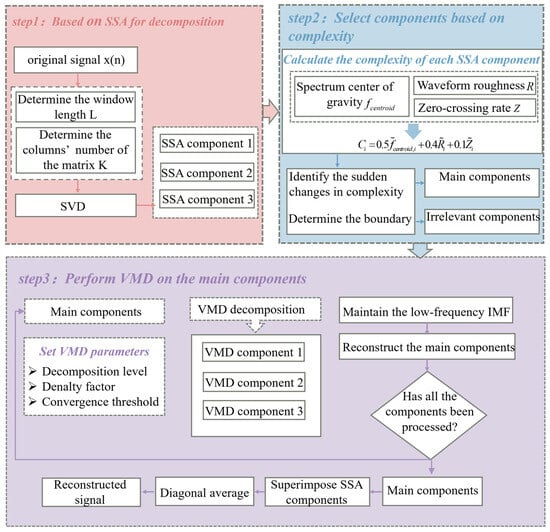
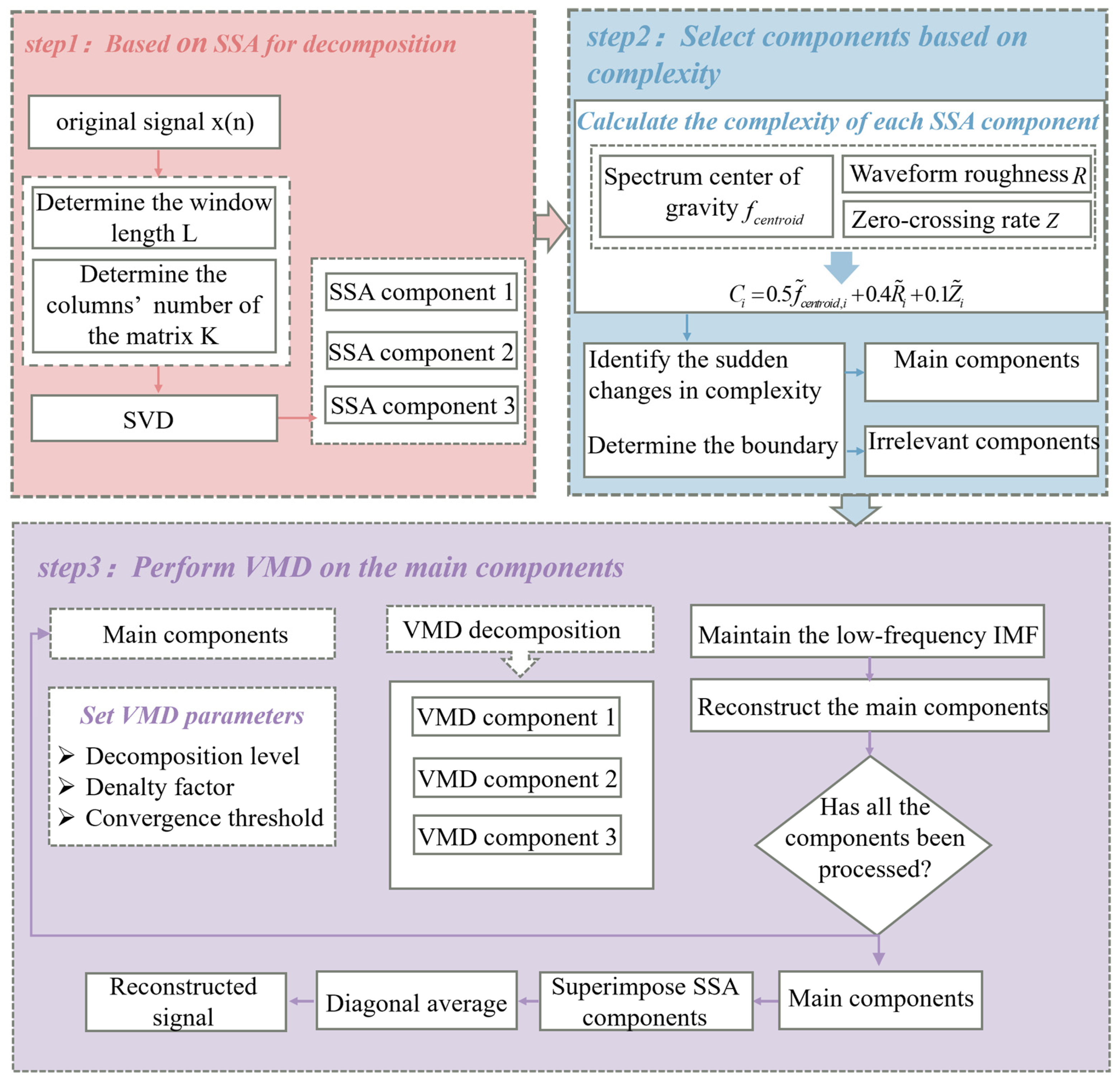
The overall process of the CM-SSA-VMD algorithm is as follows: First, a trajectory matrix is constructed from the original signal and decomposed by singular value decomposition to obtain different SSA components. Then, a component selection mechanism based on complexity mutation is introduced to determine the selection boundary of SSA components, and these components are divided into main components and irrelevant components. Next, the decomposition level and penalty factor of VMD are set, and VMD is performed on the main components to eliminate the VMD components with excessive noise, and the retained VMD components are reconstructed as SSA components. Finally, the SSA components processed by the VMD algorithm are reconstructed to obtain the denoised signal. The CM-SSA-VMD algorithm process is shown in Figure 1.

Figure 1. The process of CM-SSA-VMD.

The complexity index consists of the spectral centroid, waveform roughness, and zero-crossing rate. It characterizes the energy distribution, waveform smoothness, and local oscillation behavior of each SSA component. If the complexity undergoes an abrupt change, it indicates that the frequency and waveform characteristics of the components have undergone significant alterations. The SSA components transition from useful signal components to noise components.

The formula for calculating the spectral centroid is:

$$f_{centroid,i}={\displaystyle \frac{{{\displaystyle \sum }}_{k=1}^{N_f}{f}_k{P}_i\left(f_k\right)}{{{\displaystyle \sum }}_{k=1}^{N_f}{P}_i\left(f_k\right)}}$$

(25)

where $f_{centroid,i}$ is the spectral centroid of the $i$th SSA component, $f_k$ is the $k$th frequency point, $P_i\left(f_k\right)$ is the spectral energy of the current component at $f_k$.

The numerator of the waveform roughness expression is the root mean square of the first-order difference of the amplitudes of all adjacent sampling points in the SSA component, which reflects the average change between each adjacent sampling point. The denominator is the root mean square of the amplitude of each component, which reduces the influence of amplitude differences among components on the roughness value. The expression for waveform roughness is:

$$R_i={\displaystyle \frac{\sqrt{\frac{1}{N-1}{{\displaystyle \sum }}_{n=1}^{N-1}{\left[R{C}_i\left(n+1\right)-R{C}_i\left(n\right)\right]}^2}}{\sqrt{\frac{1}{N}{{\displaystyle \sum }}_{n=1}^{N}R{C}_i^2\left(n\right)}+\epsilon }}$$

(26)

where $R_i$ is the waveform roughness of the $i$th SSA component, $R{C}_i\left(n\right)$ is the amplitude of th $n$th sample in the $i$th SSA component, $N$ is the total number of samples in the current component, and $\epsilon$ is a very small positive number to prevent division by zero.

The zero-crossing rate reflects the oscillation frequency of the signal. A higher zero-crossing rate indicates the waveform has large local fluctuations, while a lower zero-crossing rate indicates slower waveform variation:

$$Z_i={\displaystyle \frac{1}{N-1}}{\displaystyle {\displaystyle \sum }_{n=1}^{N-1}}I[R{C}_i\left(n\right)\cdot R{C}_i\left(n+1\right)<0]$$

(27)

where $Z_i$ is the zero-crossing rate of the $i$th SSA component. When $R{C}_i\left(n\right)\cdot R{C}_i\left(n+1\right)<0$ is satisfied, $I[R{C}_i\left(n\right)\cdot R{C}_i\left(n+1\right)<0]=1$, otherwise, $I[R{C}_i\left(n\right)\cdot R{C}_i\left(n+1\right)<0]=0$.

The spectral centroid, waveform roughness, and zero-crossing rate are normalized separately and assigned different weights. The final formula for calculating the complexity is as follows:

To eliminate the differences caused by varying numerical ranges and dimensions among the three indicators—spectral centroid, waveform roughness, and zero-crossing rate—and to enable a reasonable calculation of complexity, each indicator is individually normalized using Min–Max normalization:

$${\tilde{f}}_{centroid,i}={\displaystyle \frac{f_{centroid,i}-{\min }_d(f_{centroid,d})}{{\max }_d(f_{centroid,d})-{\min }_d(f_{centroid,d})}}$$

(28)

$${\tilde{R}}_i={\displaystyle \frac{R_i-{\min }_d(R_d)}{{\max }_d(R_d)-{\min }_d(R_d)}}$$

(29)

$${\tilde{Z}}_i={\displaystyle \frac{Z_i-{\min }_d(Z_d)}{{\max }_d(Z_d)-{\min }_d(Z_d)}}$$

(30)

where ${\tilde{f}}_{c,i}$, ${\tilde{R}}_i$ and ${\tilde{Z}}_i$ are the normalized spectral centroid, waveform roughness, and zero-crossing rate, respectively.

When the signal contains significant noise, energy changes noticeably and the waveform exhibits irregular fluctuations, with distinct local variations between sampling points; so higher weights should be assigned to spectral centroid and waveform roughness. Clean ultrasonic signals also display periodic oscillations, so relying solely on zero-crossing rate to distinguish effective signals from noise yields poor results; thus, a lower weight should be assigned to the zero-crossing rate. This paper applied three weight combinations—(0.5, 0.4, 0.1), (0.4, 0.5, 0.1), and (0.4, 0.4, 0.2)—to denoise a waveform signal with a center frequency of 5 MHz and a signal-to-noise ratio (SNR) of 0 dB. The results showed that the combination (0.5, 0.4, 0.1) achieved the highest SNR of 14.3068 dB. Therefore, after normalization, the spectral centroid, waveform roughness, and zero-crossing rate were assigned weights of 0.5, 0.4, and 0.1, respectively. The final complexity calculation formula is:

$$C_i=0.5{\tilde{f}}_{centroid,i}+0.4{\tilde{R}}_i+0.1{\tilde{Z}}_i$$

(31)

where $C_i$ is the complexity index of the $i$th SSA component.

To determine the mutation positions of complexity, compute the difference in complexity between adjacent components:

$$△C_i=\left|C_{i+1}-C_i\right|$$

(32)

The position with the greatest complexity difference is the mutation position:

$$i=\max △C_i$$

(33)

If $C_{i+1}$ undergoes an abrupt change relative to $C_i$, the cutoff component is determined as $u_i\left(t\right)$ (with the main component being $u_1\left(t\right)$−$u_i\left(t\right)$).

3. Experimental Setup

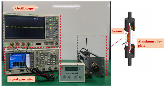
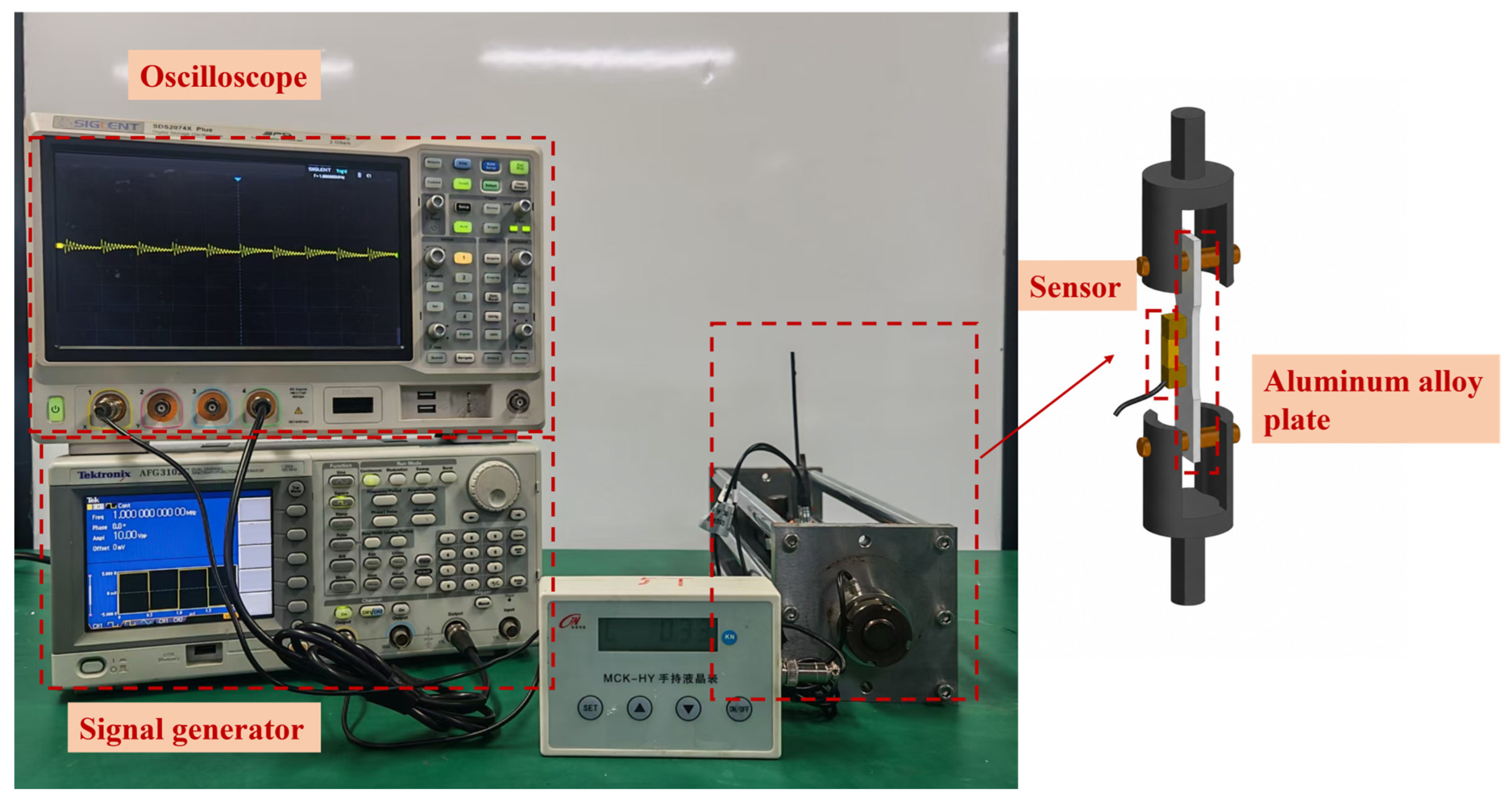
Figure 2 shows the LCR-wave-based experimental system developed for measuring residual stress. The system consists of a loading device, an ultrasonic transducer, a signal generator (AFG3102C, Tektronix, Beaverton, OR, USA), an oscilloscope (SDS2074X, Siglent, Shenzhen, China), and a 7-series aluminum alloy plate. Among them, the loading device and the ultrasonic transducer were both independently developed. The frequency of the transducer is 5 MHz, the chip size is 8 mm × 8 mm, and the wedge angle is 20°.

Figure 2. The stress measurement experimental system.

During the experiment, the stretching machine applied different stretching loads to the sheet. The signal generator produced a square wave pulse signal with a frequency of 5 MHz and a period of 4, and transmitted it to the ultrasonic transducer. The transmitting and receiving transducers were fixed on the surface of the sheet by wedges, and a layer of oil was evenly applied as a coupling agent on the contact surface between the wedges and the sheet. The distance between the ultrasonic incidence point and the receiving point was 15 mm. The transmitting transducer excited the LCR wave in the near surface layer of the sheet, and the receiving transducer converted the received ultrasonic vibration into an electrical signal. The oscilloscope displayed and stored the ultrasonic signal at a sampling interval of 1 ns.

To verify the accuracy of stress measurement under different excitation voltages using this method, experiments were conducted with 5 sets of different excitation voltages: 10 V, 5.2 V, 3.3 V, 1.2 V and 0.5 V. The measurements were carried out at 25 °C. The 7-series aluminum alloy plate used had a yield strength of at least 400 MPa and a cross-sectional area of 130 mm². To prevent plastic deformation of the specimen and ensure experimental safety, the tensile load was set from 0 to 23.4 kN. After the target load was reached, it was maintained for 120 s until it stabilized, and then the echo signals were collected. The echo signals were denoised, and the cross-correlation time delay estimation algorithm was used to calculate the ultrasonic propagation time delay. Finally, the stress was calculated according to Equation (6).

This experiment is a method validation conducted under external stress conditions, with the focus being on verifying the signal processing and stress measurement accuracy of the CM-SSA-VMD method at low excitation voltages, rather than directly measuring the residual welding stress. The externally applied tensile stress cannot fully represent the true situation of the actual residual stress field.

4. Results and Discussion

4.1. Denoising Based on CM-SSA-VMD

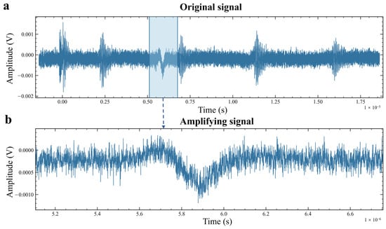
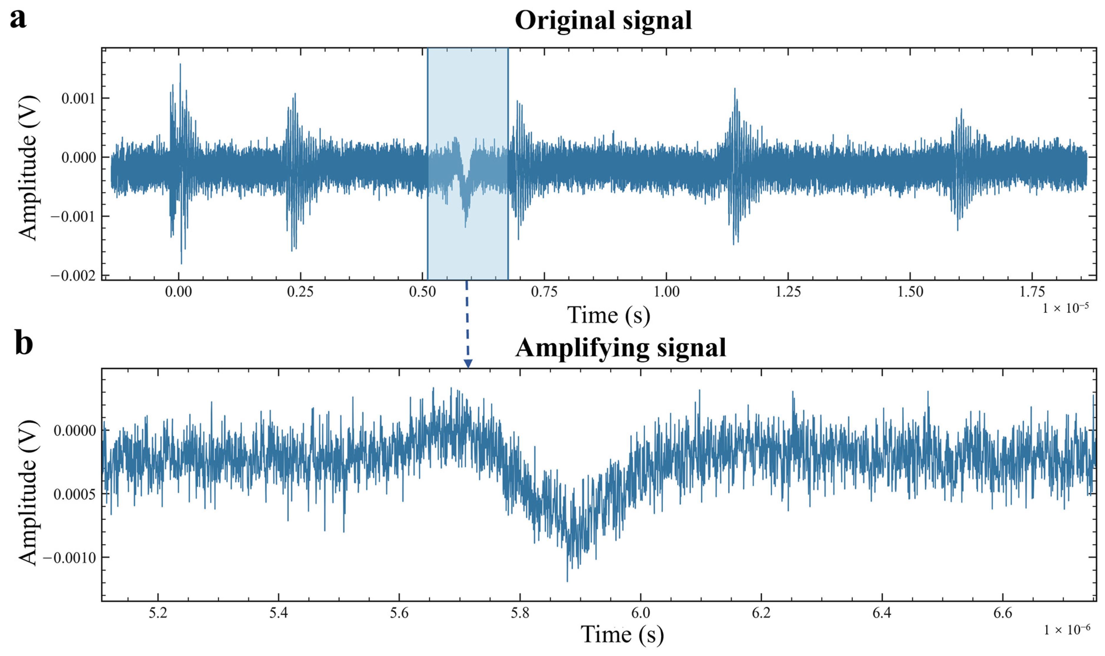
To validate the denoising performance of the proposed algorithm, the experimental setup described in Section 3 was used to collect ultrasonic signals. For this validation, an ultrasonic signal acquired at an excitation voltage of 0.5 V and a center frequency of 5 MHz was selected. Figure 3 shows the original ultrasonic signals collected under this condition. It is clearly observable that the main characteristics of the effective echoes are as follows, but the noise amplitude is relatively high, and some of it masks the effective echoes.

Figure 3. The ultrasonic waveform under a 0.5 V excitation voltage. (a) An ultrasonic signal with an excitation voltage of 0.5 V and a center frequency of 5 MHz. (b) The first echo of the ultrasound.

The collected signals were subjected to SSA decomposition. Before the decomposition, in order to determine the window length $L$, while keeping other parameters unchanged, $L$ was set to 100, 200, 300, 400, 500 and 600 respectively. Three groups of ultrasonic simulation signals with a center frequency of 5 MHz, an SNR of 0 dB and independent noise were processed. The results are shown in Table 1. When $L$ was set to 500, the SNR was the highest and the RMSE was the lowest, and the standard deviation is also smaller. This indicates that the noise variation has a relatively small impact on the performance of the algorithm, and it has good repeatability and stability. Therefore, 500 was finally selected as the window length $L$.

Table 1. The denoising results with different window lengths.

Window Length	SNR (dB, Mean ± Standard Deviation)	RMSE (Mean ± Standard Deviation)
100	11.8991 ± 0.8386	0.0930 ± 0.0087
200	14.4301 ± 0.6816	0.0694 ± 0.0055
300	15.4647 ± 0.8825	0.0617 ± 0.0063
400	16.7623 ± 2.1798	0.0542 ± 0.0132
500	17.6396 ± 0.9558	0.0480 ± 0.0053
600	17.3677 ± 0.5973	0.0494 ± 0.0034

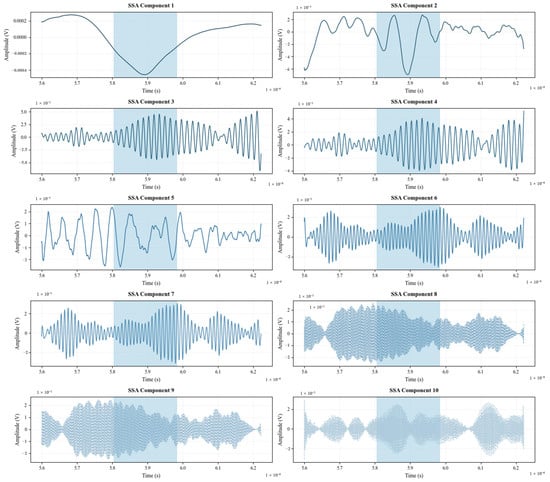
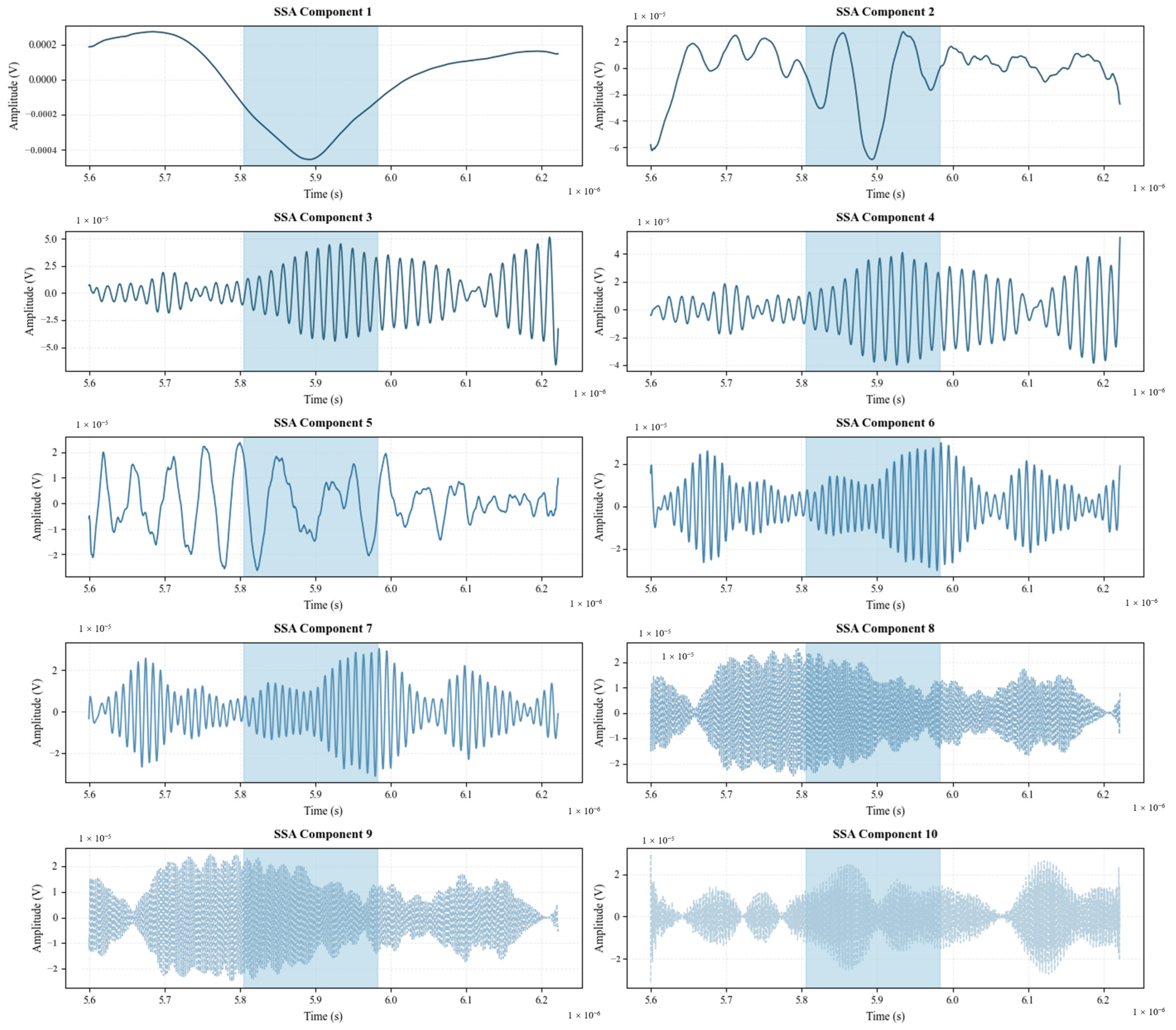
Figure 4 shows the first 10 components obtained from the SSA decomposition of the ultrasonic signal. Among them, the blue part in the picture is the main part of the first echo. Components 1–2 have relatively low frequencies and slow fluctuations. Components 3–4 have higher frequencies and regular oscillations, showing clear ultrasonic signal characteristics. Component 5 shows irregular fluctuations and peaks, while retaining some useful ultrasonic features, and it is difficult to determine whether it contains more ultrasonic features or noise features; components 6–7 have even higher frequencies, but they have periodicity and smooth waveforms; components 8–10 have significantly increased oscillation density and decreased smoothness, and it is speculated that they contain a large amount of high-frequency noise. According to Equations (25)–(31), the cutoff component is determined, as shown in Table 2. An abrupt change in complexity occurs between Components 7 and 8. Therefore, Component 7 is identified as the cutoff boundary. Components 1–7 are retained for signal reconstruction, whereas Components 8–10 are discarded.

Figure 4. SSA components. The blue shaded region indicates the main portion of the ultrasonic wave.

Table 2. Complexity indicators after normalization of different SSA components.

Component	Spectral Centroid	Waveform Roughness	Zero-Crossing Rate	Complexity	Retain
1	0.000	0.0000	0.0000	0.0000	True
2	0.0107	0.0003	0.0147	0.0069	True
3	0.0827	0.0119	0.0848	0.0546	True
4	0.0829	0.0121	0.0838	0.0547	True
5	0.0252	0.0017	0.0355	0.0168	True
6	0.1292	0.0294	0.1351	0.0899	True
7	0.1295	0.0294	0.1360	0.0901	True
8	0.6462	0.4843	0.5493	0.5716	False
9	0.6460	0.4852	0.5463	0.5717	False
10	1.0000	1.0000	1.0000	1.0000	False

To determine the parameters of VMD, the range of the decomposition layer number was set from 2 to 7, and the penalty factors $\alpha$ were 500, 1000, 1500 and 2000; the Lagrange multipliers $\tau$ were 0, 0.1, 0.2, 0.3 and 0.4. The above parameters were combined for testing. Each combination was used to perform noise reduction on three simulated ultrasound signals with center frequencies of 5 MHz but different SNRs (SNRs were 0 dB, 5 dB and 10 dB). The top five best combinations of the final results are shown in Table 3. It can be seen that when the decomposition layer number is 5, the penalty factor $\alpha$ is 1000; and the Lagrange multiplier $\tau$ is 0.1, the SNR is the highest and the RMSE is the lowest. Therefore, the above parameters were used to perform VMD on the SSA components.

Table 3. Denoising results for the five best-performing VMD parameter combinations.

Decomposition Layer Number	Penalty Factors	Lagrange Multiplier	SNR (dB, Mean ± Standard Deviation)	RMSE (Mean ± Standard Deviation)
5	1000	0.1	15.3451 ± 1.8711	0.0662 ± 0.0114
4	1000	0.4	15.2763 ± 1.8385	0.0664 ± 0.0113
5	1000	0	15.2357 ± 1.8349	0.0670 ± 0.0113
4	1000	0.2	15.2217 ± 1.7315	0.0671 ± 0.0109
4	1000	0.1	15.2110 ± 1.6927	0.0672 ± 0.0106

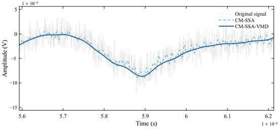
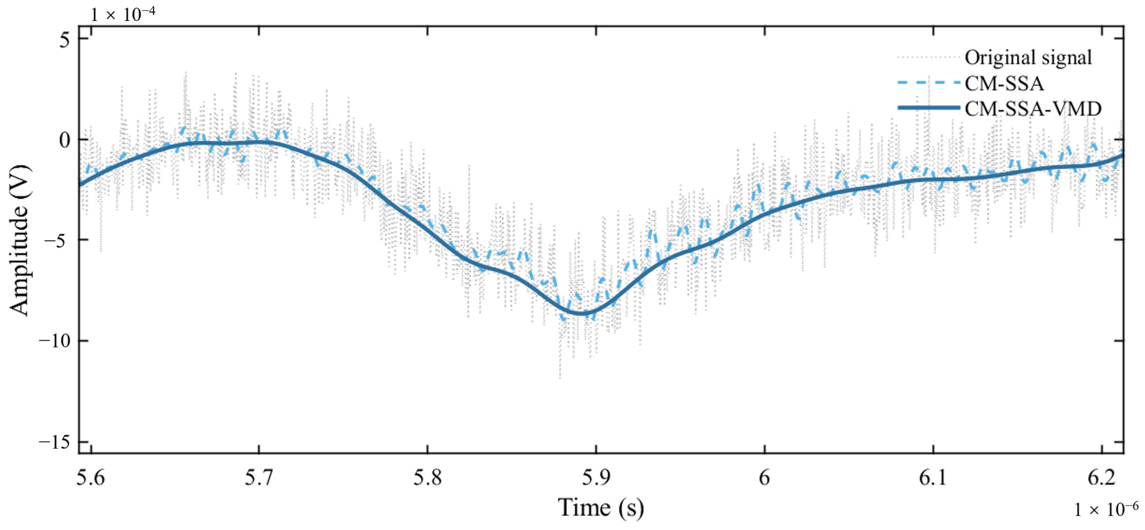
Figure 5 compares the denoising performance of the CM-SSA-VMD algorithm and the complexity-mutation-based adaptive singular spectrum analysis (CM-SSA) algorithm. For subsequent analysis, the signal processed by the CM-SSA-VMD algorithm is denoted as Signal A, and the signal processed by the CM-SSA algorithm is denoted as Signal B. Compared with the original signal, both algorithms reduce high-frequency spikes. However, Signal A has greater smoothness and fewer peaks. Although Signal B preserves the main trend of the signal, its local fluctuations are larger than those of Signal A, indicating that it still contains some residual noise. The SNR values of signals A and B are 13.10 dB and 12.25 dB respectively, which intuitively indicates that the denoising effect of the CM-SSA-VMD method is better than that of the CM-SSA method. These results show that introducing further VMD after the CM-SSA algorithm can suppress noise more effectively and improve the denoising performance for low-voltage excitation ultrasonic signals.

Figure 5. Denoising performance of CM-SSA method and CM-SSA-VMD method.

4.2. Algorithm Comparison

In this section, a clean simulated ultrasound signal is first constructed as the reference signal, and different intensities of noise are added to it to create noisy signals with SNR values of 0 dB, 2 dB, 5 dB, 10 dB, and 15 dB. The above noisy signals are then denoised using CM-SSA-VMD, GWO-VMD-WT, VMD and FIR filters, and the SNR and RMSE are used as evaluation metrics to compare the performance of the four algorithms. In the calculation of RMSE, the reference signal is the initial clean ultrasound signal.

The CM-SSA-VMD algorithm parameters are set as described in Section 4.1. To determine the parameters of the GWO-VMD-WT algorithm, the population size was set to 5, 10, and 15 respectively, and the number of iterations was set to 5, 10, and 15 respectively. The two sets of parameters were combined. For each combination, the decomposition layers, penalty factor $\alpha$, and Lagrange multiplier $\tau$ were searched, and the 0 dB simulated ultrasound signal mentioned in Section 4.1 was independently denoised three times. From Table 4, it can be seen that when the population size is 10 and the number of iterations is 15, the SNR is the highest and the SMRE is the lowest. At this time, the decomposition layers and penalty factor $\alpha$ are 6, and the Lagrange multiplier $\tau$ is 1975.4087. Therefore, GWO-VMD-WT adopts the above parameters. The standalone VMD algorithm does not use SSA for initial decomposition. To improve frequency decomposition accuracy, the number of VMD components is set to 7, and the first three modes are retained for reconstruction. The other parameters are the same as those in Section 4.1. In order to find more suitable filter parameters, the filter order was set to 50, 70, 100 and 150, and each was combined with three passbands: 4–6 MHz, 4.25–5.75 MHz and 4.5–5.5 MHz. Each combination separately performed noise reduction processing on the simulated ultrasound signals mentioned in Section 4.1 (with SNR values of 0 dB, 5 dB, and 10 dB respectively). From Table 5, it can be seen that when the passband is 4.5–5.5 MHz and the filter order is 100 order, the effect is the best. Therefore, the FIR filter is set as a 100th-order band-pass filter. The upper and lower cut-off frequencies are respectively set at 5.5 MHz and 4.5 MHz, with a bandwidth of 1 MHz. The denoising performance and results of the four algorithms are shown in Figure 6 and Figure 7.

Table 4. Denoising results for the five best-performing GWO–VMD–WT parameter combinations.

Population Size	Iterations	Decomposition Level	Penalty Factor	Lagrangian Multiplier	SNR (dB, Mean ± Standard Deviation)	RMSE (Mean ± Standard Deviation)
10	15	6	6	1975.4807	17.1340 ± 0.2156	0.0513 ± 0.0015
5	15	6	6	502.6575	17.0452 ± 0.2118	0.0517 ± 0.0015
5	10	6	6	500.0000	17.0231 ± 0.2231	0.0518 ± 0.0017
5	5	6	6	869.0040	17.0067 ± 0.2506	0.0519 ± 0.0119
5	15	6	6	1687.3144	16.9741 ± 0.2539	0.0521 ± 0.0119

Table 5. Denoising results for the five best-performing FIR filter parameter combinations.

Filter Order	Passband	SNR (dB, Mean ± Standard Deviation)	RMSE (Mean ± Standard Deviation)
100	4.5–5.5	16.9423 ± 0.2362	0.0555 ± 0.0015
100	4.25–5.75	16.9421 ± 0.2363	0.0555 ± 0.0015
70	4.5–5.5	16.9382 ± 0.2369	0.0556 ± 0.0016
100	4–6	16.6851 ± 0.3074	0.0563 ± 0.0024
70	4.25–5.75	16.6818 ± 0.3079	0.0565 ± 0.0025

Figure 6. Performance comparison under different initial SNR values.

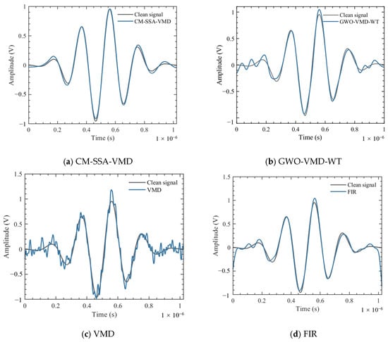
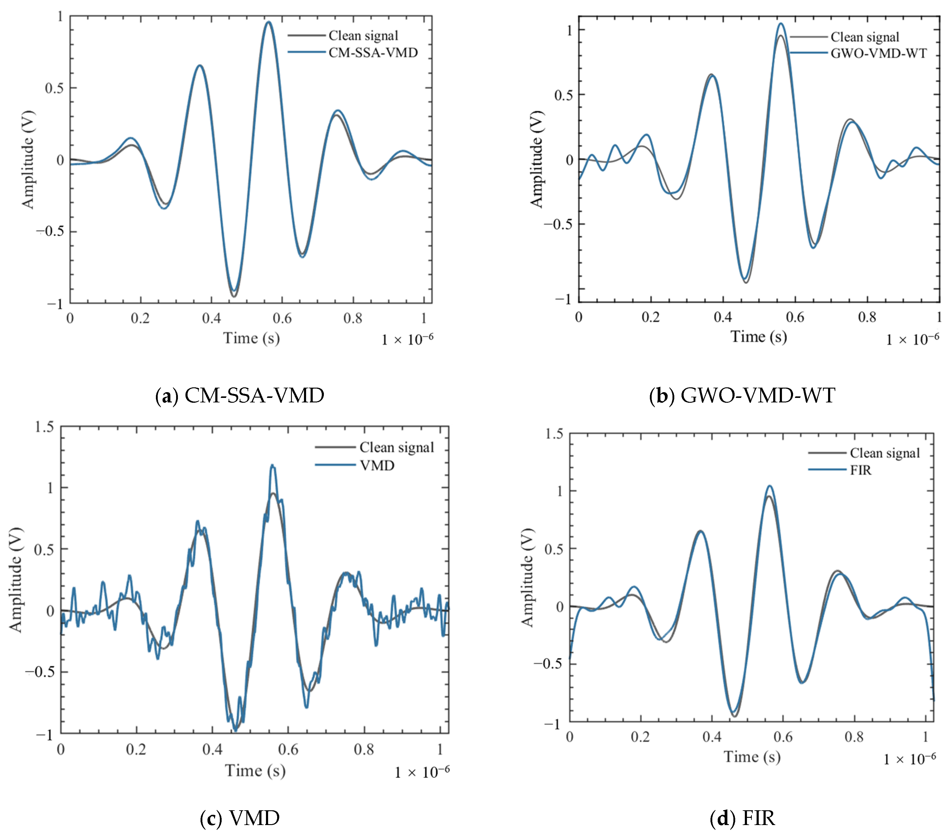
Figure 7. The waveform after noise reduction of the 0 dB signal.

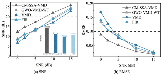
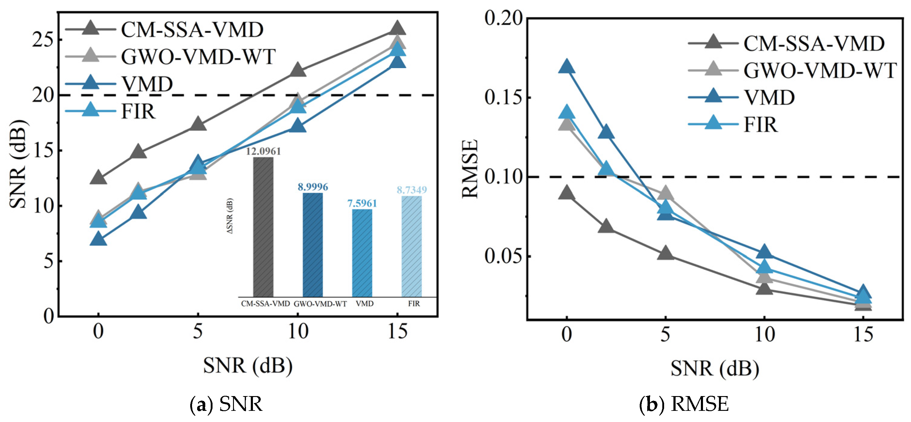
The line plot in Figure 6a shows the SNR values after denoising by the four algorithms, while the bar graph shows the average increment of SNR; Figure 6b shows the RMSE values after denoising by the four algorithms. Under different noise levels, the signals processed by the CM-SSA-VMD algorithm achieve the highest SNR, with an average improvement of more than 12 dB. The RMSE is the lowest and remains below 0.1. Specifically, when the initial SNR is 10 dB, the signal processed by the CM-SSA-VMD algorithm achieves an SNR above 20 dB, reaching a relatively good level, whereas the SNRs obtained by the GWO-VMD-WT, VMD and the FIR algorithms remain below 20 dB. For the ultrasonic signal with an initial SNR of 0 dB, the CM-SSA-VMD algorithm increases the SNR by 12.4124 dB and achieves an RMSE of 0.0891. This indicates that the algorithm effectively suppresses noise and that the reconstructed signal closely matches the clean signal. The average SNR increments of the GWO-VMD-WT, VMD and FIR algorithms are approximately 3.1 dB, 4.5 dB and 3.4 dB lower than those of the CM-SSA-VMD algorithm, indicating relatively limited denoising performance.

Figure 7 shows the waveforms after denoising the 0 dB signal using the four algorithms. The signal processed by the CM-SSA-VMD algorithm is smooth and follows the trend of the clean signal. The signal after GWO-VMD-WT processing is smoothed, but there is a deviation at the peak. Fluctuations also occur at the beginning and end stages of the signal. Although the signal processed by the VMD algorithm can maintain the main signal trend, the denoised signal still contains many spikes and noticeable residual noise. The signal processed by the FIR algorithm is smoother than that processed by the VMD algorithm, but there are fluctuations and deviations at the beginning and end of the signal, and the signal trend is inconsistent with the clean signal. In order to more comprehensively evaluate the noise reduction effects of the four methods, the Pearson correlation coefficient (PCC) and TOF deviation of the denoised signals were calculated. The waveform retention ability and TOF calculation accuracy of the three methods were evaluated. As can be seen from Table 6, the signal after processing with CM-SSA-VMD has the highest PCC, and the TOF deviation is 3 ns, indicating that this method can better preserve the original waveform features and will not cause significant time offsets in the TOF calculation. Therefore, CM-SSA-VMD can more effectively suppress noise interference while preserving the main signal features.

Table 6. The PCC and flight time accuracy after denoising using different methods.

Algorithm	PCC	ΔTOF (ns)
CM-SSA-VMD	0.9971	3
GWO-VMD-WT	0.9896	4
VMD	0.9732	4
FIR	0.9723	5

4.3. Analysis of Stress Measurement Errors

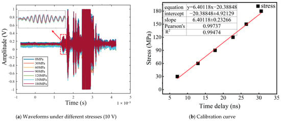
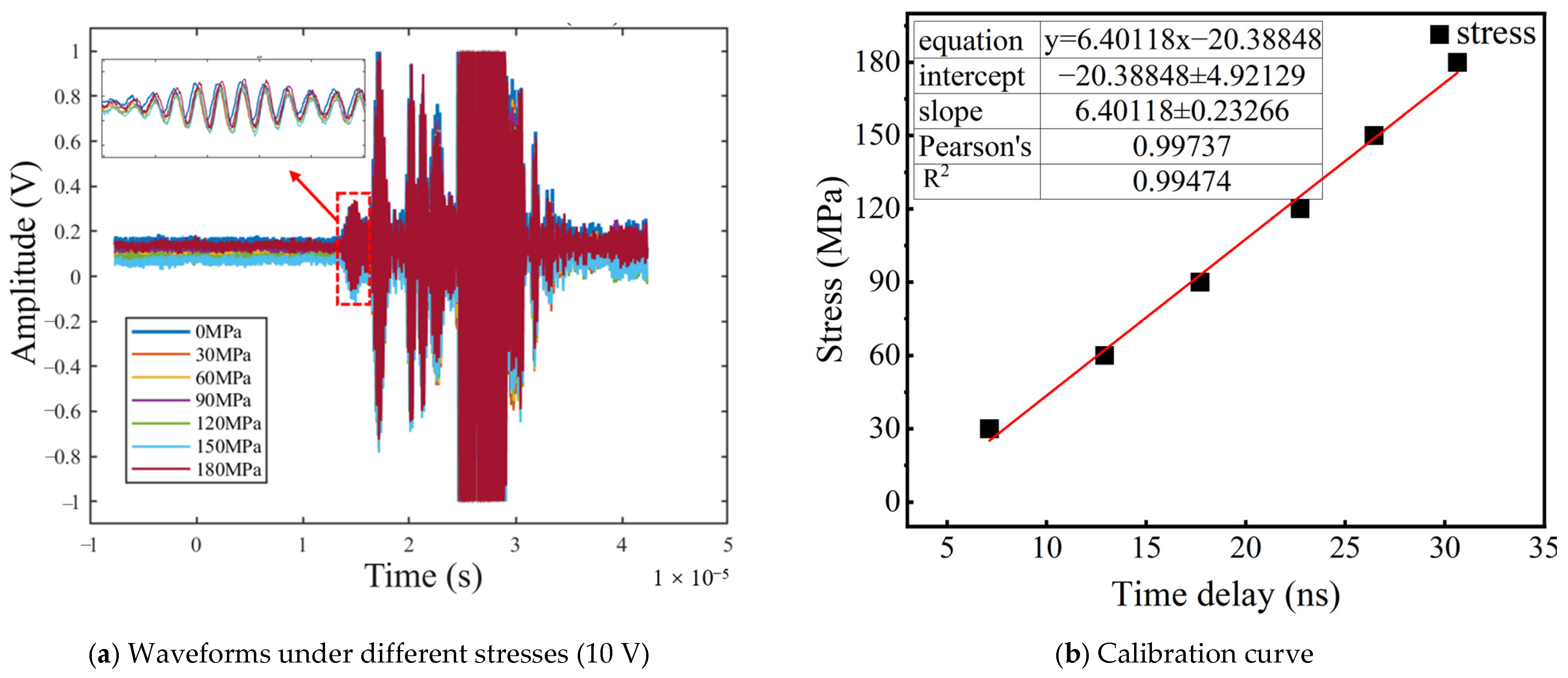
Figure 8 presents the calibration data of the sample based on a 10 V excitation voltage. Figure 8a shows the ultrasonic signal under a 10 V excitation voltage. It can be clearly observed that the signal amplitude is high and there is almost no noise interference; thus, under this condition, six stress levels of 30, 60, 90, 120, 150 and 180 MPa were used for calibration, and a highly linear calibration curve with excellent performance was obtained as shown in Figure 8b. The fitted equation is y = 6.40118x − 20.38848, with a Pearson correlation coefficient r = 0.99737 and a coefficient of determination R² = 0.99474, indicating a strong linear relationship between the two variables. The slope of the calibration curve, i.e., the stress coefficient K = 6.40118 MPa/ns, has a standard error of 0.23266 MPa/ns and a 95% confidence interval of 5.7552–7.0471 MPa/ns, further demonstrating good stability of this coefficient. Since the calibration coefficient is related to the material itself and is independent of the excitation voltage, it will be used as K = 6.40118 MPa/ns in the subsequent stress tests conducted under different excitation voltages.

Figure 8. Calibration curve of stress coefficient. The red box in (a) highlights the received ultrasonic echo.

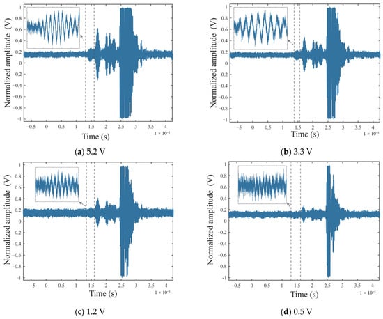
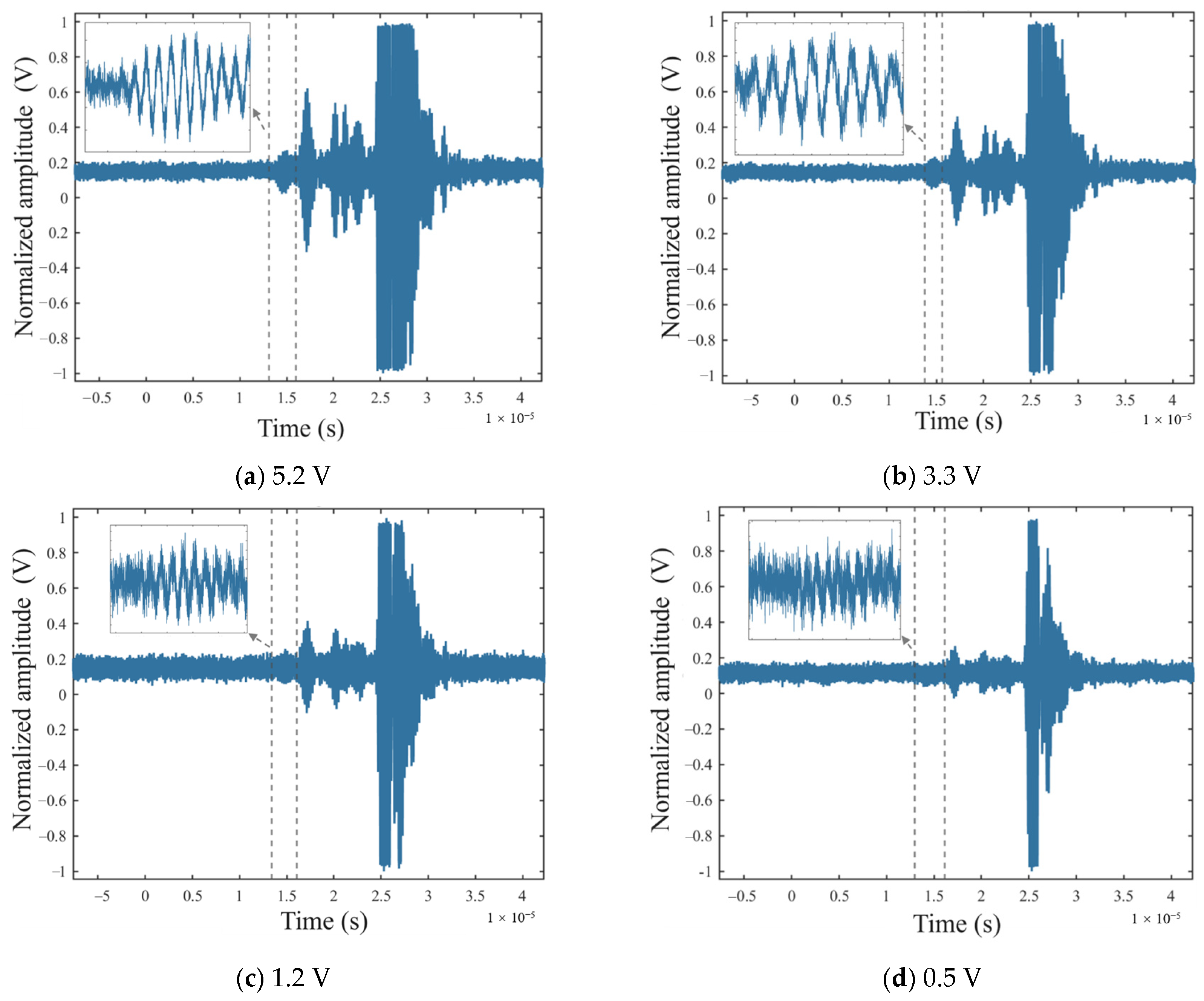
Figure 9a–d shows the ultrasonic echo signals collected when the excitation voltage is 5.2 V, 3.3 V, 1.2 V, and 0.5 V. As the excitation voltage decreases, the noise gradually increases. Under a 5.2 V excitation voltage, the main echo waveform remains clear. When the excitation voltage is reduced to 0.5 V, the collected signal shows dense random fluctuations, and the noise almost completely overwhelms the main echo signal. Table 7 presents the SNRs of the LCR wave signals at different excitation voltages. At 5.2 V, the SNR is 12.45 dB. When the excitation voltage decreases to 0.5 V, the SNR decreases by 10.36 dB to only 2.09 dB.

Figure 9. Ultrasound echo signals under different low excitation voltages.

Table 7. SNR at different excitation voltages.

Excitation Voltage (V)	SNR
5.2	12.45
3.3	10.56
1.2	7.79
0.5	2.09

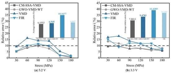
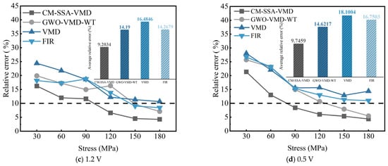
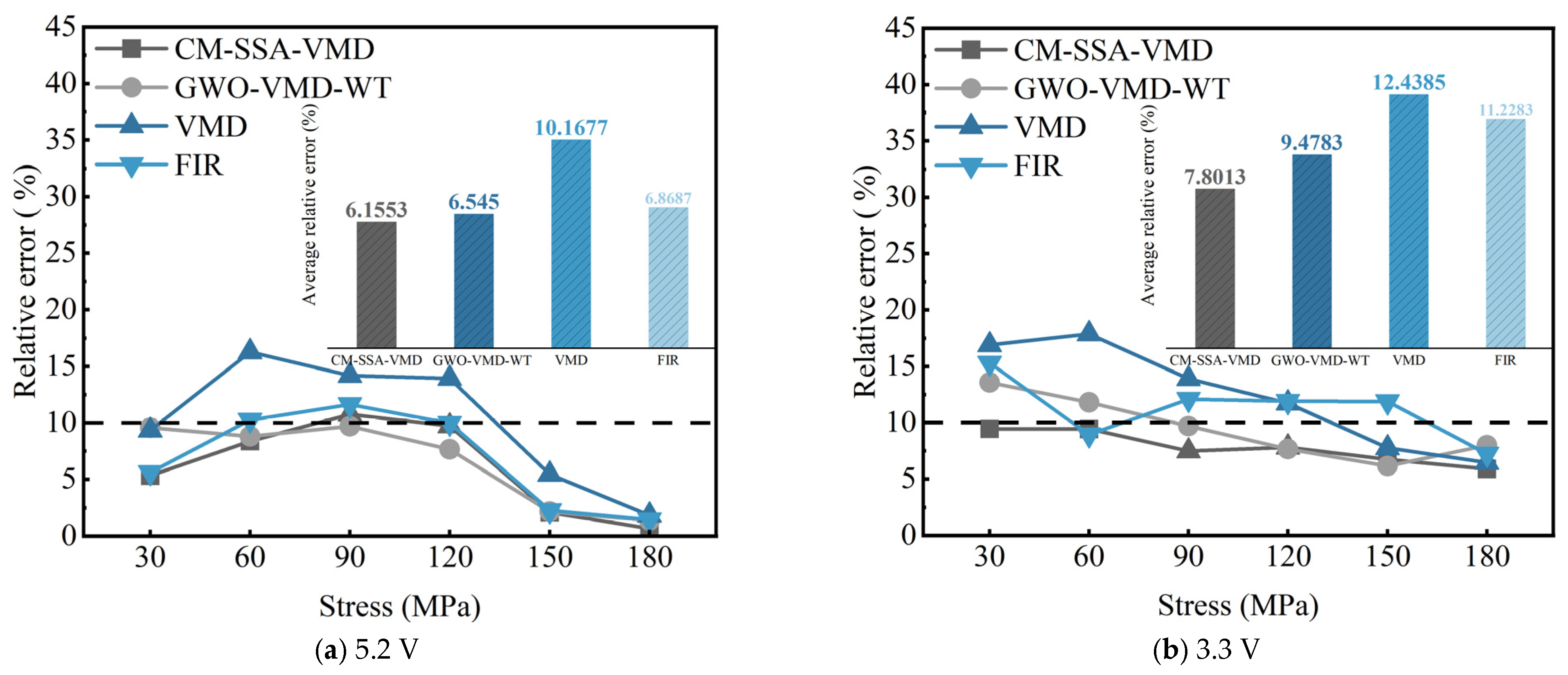
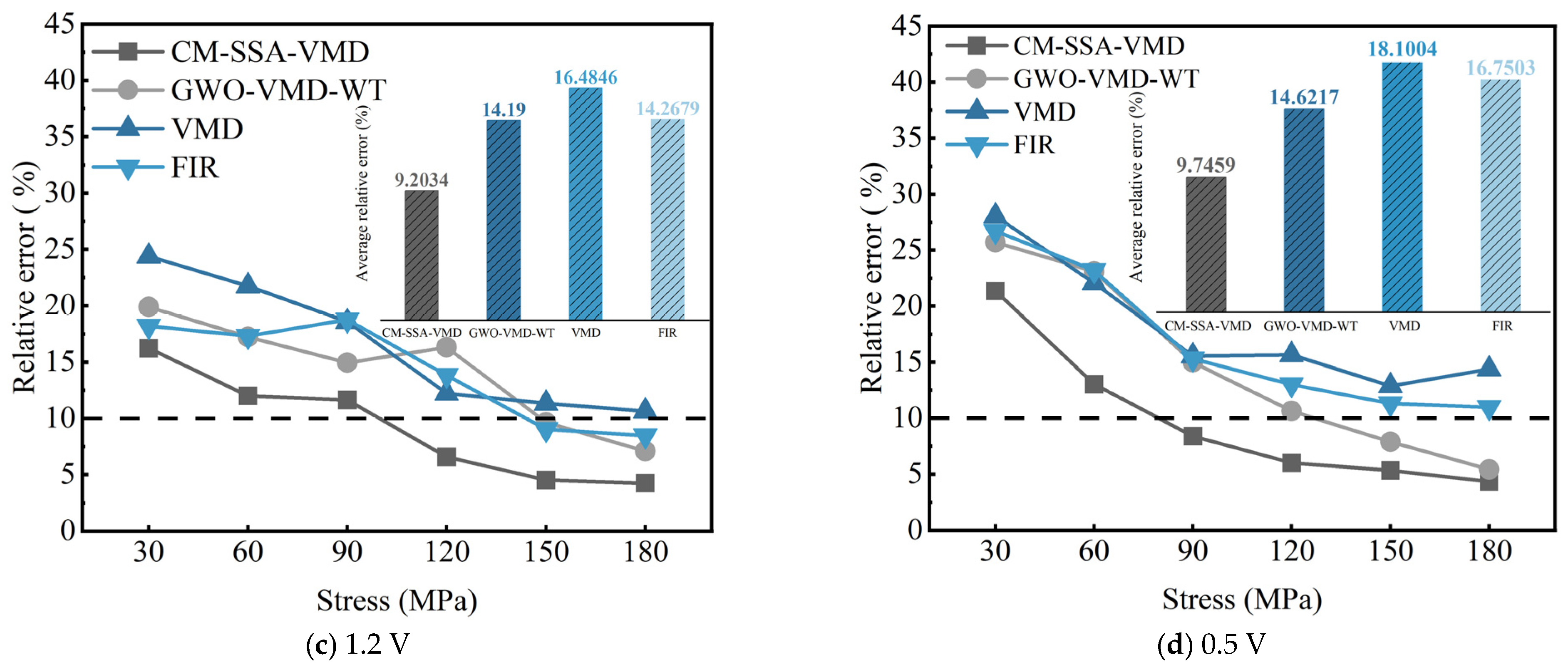
To evaluate the improvement effect of the proposed denoising algorithm on stress measurement accuracy, the CM-SSA-VMD algorithm, the GWO-VMD-WT algorithm, the VMD algorithm, and the FIR filter are applied to denoise the LCR wave signals under different excitation voltages, and stress measurements are conducted based on the denoised signals. Different methods were used to measure stress, and the measurements were repeated three times. The average accuracy of the stress measurements for the four final methods is shown in Figure 10, and the error range is presented in Table 8.

Figure 10. Stress measurement accuracy under different low excitation voltages.

Table 8. Stress measurement error.

Excitation Voltage (V)	Stress (MPa)	CM-SSA-VMD (%, Mean ± Standard Deviation)	GWO-VMD-WT (%, Mean ± Standard Deviation)	VMD (%, Mean ± Standard Deviation)	FIR (%, Mean ± Standard Deviation)
5.2	30	5.3293 ± 0.2493	9.5800 ± 0.3463	9.3313 ± 0.37467	5.6234 ± 0.3827
	60	8.3731 ± 0.2319	8.8000 ± 0.3314	16.2674 ± 0.6933	10.2674 ± 0.3221
	90	10.7712 ± 0.2237	9.6900 ± 0.3561	14.1894 ± 0.5628	11.6290 ± 0.3671
	120	9.7173 ± 0.2614	7.6600 ± 0.3497	13.9314 ± 0.5173	9.9840 ± 0.2745
	150	2.0838 ± 0.0608	2.1600 ± 0.0746	5.4550 ± 0.3073	2.2545 ± 0.1021
	180	0.6576 ± 0.0593	1.3800 ± 0.0837	1.8317 ± 0.0983	1.4540 ± 0.0722
3.3	30	12.0384 ± 0.3093	20.2700 ± 0.8301	22.0384 ± 0.9026	18.7051 ± 0.7624
	60	12.7478 ± 0.3106	14.2800 ± 0.6294	20.8107 ± 0.8673	17.4774 ± 0.6947
	90	8.4746 ± 0.2437	10.2700 ± 0.3582	16.8452 ± 0.7953	14.9109 ± 0.5331
	120	5.4051 ± 0.1517	9.7700 ± 0.3726	16.4447 ± 0.8275	8.5727 ± 0.3094
	150	6.9365 ± 0.1583	7.3600 ± 0.3582	11.3945 ± 0.3998	9.4582 ± 0.2908
	180	4.8178 ± 0.1395	6.3500 ± 0.2478	10.8309 ± 0.3538	6.1226 ± 0.2873
1.2	30	16.2399 ± 0.4283	19.8900 ± 0.7138	24.3854 ± 1.2341	18.1928 ± 0.7983
	60	12.0005 ± 0.3894	17.2400 ± 0.6822	21.7468 ± 0.9475	17.3112 ± 0.6352
	90	11.6257 ± 0.3793	14.9400 ± 0.5901	18.5811 ± 0.7496	18.7528 ± 0.7809
	120	6.5818 ± 0.2961	16.3300 ± 0.6340	12.2220 ± 0.4231	13.8247 ± 0.5276
	150	4.5190 ± 0.2837	9.6500 ± 0.3819	11.3274 ± 0.3992	9.0444 ± 0.3246
	180	4.2540 ± 0.2861	7.0900 ± 0.2741	10.6452 ± 0.3752	8.4820 ± 0.2998
0.5	30	21.3717 ± 0.5218	25.7000 ± 0.9247	28.0384 ± 1.5078	26.7051 ± 1.3896
	60	13.0253 ± 0.3216	23.0900 ± 0.8714	22.0745 ± 1.3281	23.2000 ± 1.1038
	90	8.3923 ± 0.2761	14.9900 ± 0.4831	15.5647 ± 0.7861	15.3041 ± 0.5941
	120	6.0096 ± 0.2459	10.6500 ± 0.4298	15.6590 ± 0.8029	13.0096 ± 0.4710
	150	5.3321 ± 0.2388	7.8900 ± 0.3855	12.8853 ± 0.5083	11.3103 ± 0.3985
	180	4.3448 ± 0.2130	5.4100 ± 0.2946	14.3809 ± 0.5325	10.9728 ± 0.3257

The line plot in Figure 10 shows the average relative errors at different load points for the four algorithms after three repeated measurements, while the bar graph presents the average relative errors at six load points. The measurement errors of all four algorithms increase as the excitation voltage decreases. However, at the same excitation voltage, the CM-SSA-VMD algorithm produced lower errors than the other three algorithms. Specifically, as the excitation voltage decreases from 5.2 V to 0.5 V, the average relative error of the CM-SSA-VMD algorithm increases from 6.16% to 9.75%, but remains below 10%. The GWO-VMD-WT algorithm has an average relative error of less than 10% when the operating voltage is 3.3 V or higher. However, when the excitation voltage drops to 1.2 V or lower, the average relative error exceeds 10%. For the FIR filter algorithm, the average relative error is 6.87% at 5.2 V and exceeds 10% when the excitation voltage is 3.3 V or lower. The VMD algorithm performs worse than the other three methods, with the average relative error above 10% at all excitation voltages of 5.2 V and below. Table 8 presents the average values and standard deviations of the relative errors obtained from three repeated measurements of the four algorithms under different excitation voltages and load conditions. After three measurements, the standard deviations of the four methods were generally small, almost below 1%, indicating good consistency. Compared with the other three algorithms, CM-SSA-VMD maintains a smaller degree of dispersion under different conditions, with relatively small standard deviation changes, indicating that this method also has good stability.

To verify whether a low excitation voltage can effectively reduce power consumption, the power consumption under excitation voltages of 5.2 V, 3.3 V, 1.2 V and 0.5 V was tested. As shown in Table 9, when the excitation voltage was 5.2 V, the power consumption was the highest, at 245.973 mW. As the excitation voltage decreased, the power consumption also gradually decreased. When the excitation voltage was 0.5 V, the power consumption reached the lowest, at only 13.043 mW.

Table 9. Power consumption at different voltages.

Excitation Voltage (V)	Power Dissipation (mW)
5.2	245.9730
3.3	98.9390
1.2	13.0680
0.5	13.0430

4.4. Further Validation of Residual Stress Measurement and Material Applicability

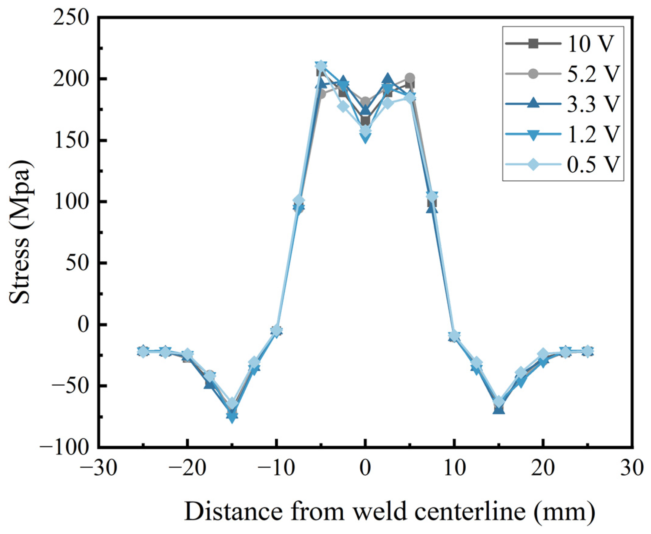
In order to further verify the applicability of CM-SSA-VMD in actual welded structural components, a sample of MIG-welded aluminum plate was used, and the longitudinal residual stress on its surface was tested along the direction perpendicular to the weld seam. The tests were conducted using five excitation voltages of 50, 5.2, 3.3, 1.2, and 0.5 V, and the test results at 50 V voltage were taken as the reference to verify the applicability of CM-SSA-VMD under low excitation voltage conditions.

As shown in Figure 11, the trends of the residual stress curves under the five excitation voltages are basically consistent. Compared with the reference results, the peak stress, the width of the stress distribution, and the transition position of tensile residual stress and compressive residual stress under the low excitation voltage did not show significant changes. The average relative errors of the four low excitation voltages were all lower than 10%, among which the average relative error at the lowest excitation voltage of 0.5 V was 9.11%. The above results indicate that for MIG-welded aluminum plates, the CM-SSA-VMD method can detect the residual stress of the welded structure using low excitation voltages.

Figure 11. Measurement of residual stress under different voltages.

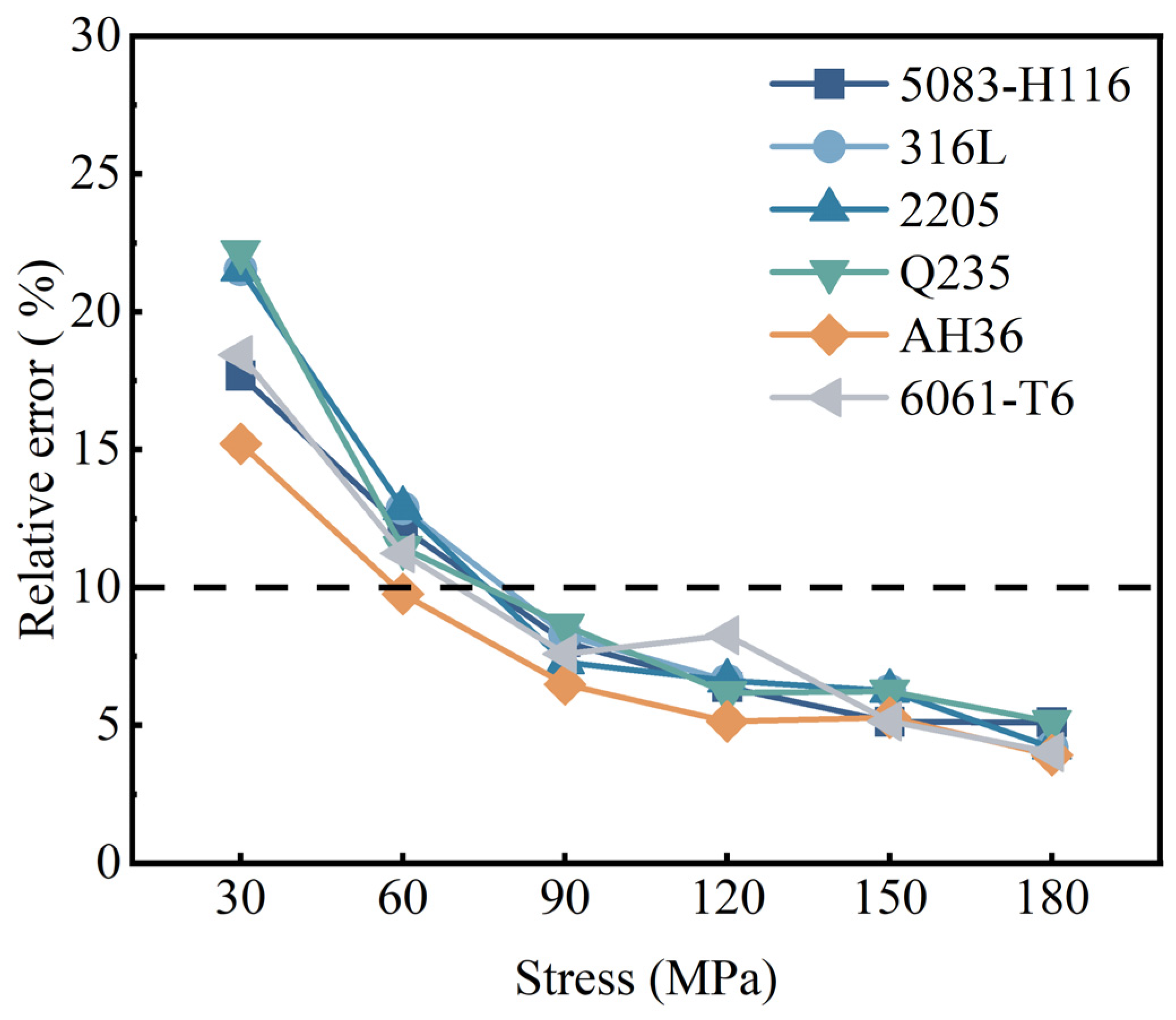
To verify the universality of this method in different materials, 5083-H116 aluminum alloy, 6061-T6 aluminum alloy, 316L austenitic stainless steel, 2205 duplex stainless steel, Q235 carbon structural steel, and AH36 high-strength shipbuilding steel were selected as samples, and experiments were conducted at room temperature.

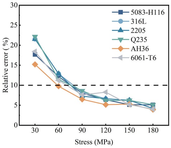
As shown in Figure 12, the average relative errors of 5083-H116, 6061-T6, 316L, 2205, Q235, and AH36 were all below 10%, being 9.08%, 9.12%, 9.95%, 9.79%, 9.92%, and 7.63% respectively. This indicates that under low-voltage excitation conditions, CM-SSA-VMD has certain applicability for these materials. However, this experiment only involved six metal materials, and the conclusions obtained are limited by the materials and testing environment, and cannot be directly generalized to other material components. In the subsequent stage, the applicability and repeatability of this method for other materials will be further verified. It should be noted that this experiment is only a test of residual stress in aluminum plate welding structures under normal temperature conditions. In the future, tests and verifications will be conducted on the welding structures of ships.

Figure 12. Stress measurement errors for different materials.

5. Conclusions

To address reduced stress measurement accuracy caused by weakened echo energy and increased noise at low excitation voltages, this paper proposes the CM-SSA-VMD algorithm. The algorithm uses a complexity index to characterize the frequency distribution, smoothness, and oscillation frequency of the SSA components, adaptively selects the reconstructed SSA components, and performs VMD on the reconstructed components to further separate the residual noise, achieving effective denoising. Through algorithm performance comparison and the stress measurement accuracy experiment, the following conclusions were obtained:

(1)

At initial SNRs ranging from 0 to 15 dB, the output SNR of the signal processed by the CM-SSA-VMD algorithm was the highest, with an average increase of more than 12 dB; the RMSE was the lowest, at less than 0.1. The average SNR increments of the VMD algorithm and the FIR filter were approximately 4.5 dB and 3.4 dB lower than that of CM-SSA-VMD.

(2)

Within the stress range of 30~180 MPa, as the excitation voltage decreased from 5.2 to 0.5 V, the average relative error of the CM-SSA-VMD algorithm increased from 6.16% to 9.75%, but remained below 10%. In contrast, the average relative error of the FIR filter exceeded 10% when the excitation voltage was no higher than 3.3 V, and the average relative error of the VMD algorithm exceeded 10% when the excitation voltage was 5.2 V or lower.

(3)

Under the excitation voltages of 5.2 V, 3.3 V, 1.2 V, and 0.5 V, as the voltage decreases, the power consumption gradually reduces. When the excitation voltage is 5.2 V, the power consumption is the highest, at 245.973 mW; when the excitation voltage is 0.5 V, the power consumption reaches the lowest, at only 13.043 mW.

(4)

The stress trends of five materials—5083-H116 aluminum alloy, 6061-T6 aluminum alloy, 316L austenitic stainless steel, 2205 duplex stainless steel, Q235 carbon structural steel, and AH36 high-strength shipbuilding steel—at a 0.5 V low voltage are consistent with the reference residual stress trends, and the average relative errors under four low excitation voltages are all below 10%.

In conclusion, CM-SSA-VMD can effectively handle ultrasonic signals with low signal-to-noise ratio, reduce the influence of noise on stress monitoring, and ensure the accuracy of stress measurement under low-power consumption conditions, providing a feasible solution for ultrasonic stress monitoring.

References

- Dong, Y.; Garbatov, Y.; Soares, C.G. Recent developments in fatigue assessment of ships and offshore structures. J. Mar. Sci. Appl. 2022, 21, 3–25. [Google Scholar] [CrossRef] [Scilit]
- Yi, M.S.; Noh, S.H.; Lee, D.H.; Seo, D.H.; Paik, J.K. Direct measurements, numerical predictions and simple formula estimations of welding-induced biaxial residual stresses in a full-scale steel stiffened plate structure. Structures 2021, 29, 2094–2105, Erratum in Structures 2021, 33, 1906. [Google Scholar] [CrossRef] [Scilit]
- Li, S.; Kim, D.K.; Benson, S. The influence of residual stress on the ultimate strength of longitudinally compressed stiffened panels. Ocean Eng. 2021, 231, 108839. [Google Scholar] [CrossRef] [Scilit]
- Mathar, J. Determination of initial stresses by measuring the deformations around drilled holes. J. Fluids Eng. 1934, 56, 249–254. [Google Scholar] [CrossRef] [Scilit]
- Nitschke-Pagel, T. Recommendations for the measurement of residual stresses in welded joints by means of X-ray diffraction—Results of the WG6-RR test. Weld. World 2021, 65, 589–600. [Google Scholar] [CrossRef] [Scilit]
- Chen, B.; Luo, C.; Xia, L.; Xu, L.; Yan, G.; Qiu, F.; Gou, G. Research on the measurement technology for pretension stress on small-sized bolts based on the piezoelectric ultrasonic resonance method. Materials 2024, 17, 5802. [Google Scholar] [CrossRef] [Scilit] [PubMed]
- Hughes, D.S.; Kelly, J.L. Second-order elastic deformation of solids. Phys. Rev. 1953, 92, 1145–1149. [Google Scholar] [CrossRef] [Scilit]
- Leon-Salamanca, T.; Bray, D.F. Residual stress measurement in steel plates and welds using critically refracted longitudinal (LCR) waves. Res. Nondestruct. Eval. 1996, 7, 169–184. [Google Scholar] [CrossRef] [Scilit]
- Kendall, O.; Paradowska, A.; Abrahams, R.; Reid, M.; Qiu, C.; Mutton, P.; Yan, W. Residual stress measurement techniques for metal joints, metallic coatings and components in the railway industry: A review. Materials 2022, 16, 232. [Google Scholar] [CrossRef] [Scilit] [PubMed]
- Beghini, M.; Grossi, T. Towards a reliable uncertainty quantification in residual stress measurements with relaxation methods: Finding average residual stresses is a well-posed problem. Exp. Mech. 2024, 64, 851–874. [Google Scholar] [CrossRef] [Scilit]
- Luo, C.; Chen, B.; Xia, L.; Xu, L.; Liu, X.; Zou, S.; Peng, D.; Gou, G. Residual stress measurement using EMAT for X80 pipeline steel: Effects of coating thickness and surface roughness under low surface preparation requirements. Materials 2024, 17, 5799. [Google Scholar] [CrossRef] [Scilit] [PubMed]
- Hwang, Y.-I.; Kim, G.; Kim, Y.-I.; Park, J.-H.; Choi, M.Y.; Kim, K.-B. Experimental measurement of residual stress distribution in rail specimens using ultrasonic LCR waves. Appl. Sci. 2021, 11, 9306. [Google Scholar] [CrossRef] [Scilit]
- Losada, M.; Olaizola, A.; Irizar, A.; Fernández, I.; Carrasco, A.; Zanden, J.V.D.; Cortés, A. UWB-based accelerometer sensor nodes for low-power applications in offshore platforms. Electronics 2024, 13, 4485. [Google Scholar] [CrossRef] [Scilit]
- Xiao, Y.; Rivandi, H.; Costa, T.L. An energy-efficient high-voltage pulser for high-frequency ultrasound medical applications. In Proceedings of the IEEE Biomedical Circuits and Systems Conference (BioCAS 2023), Toronto, ON, Canada, 19–21 October 2023; pp. 1–5. [Google Scholar] [CrossRef] [Scilit]
- Marcus, C.; Nayeem, M.O.G.; Shah, A.; Hou, J.; Viswanath, S.; Eusebio, M.; Sadat, D.; Chandrakasan, A.P.; Ozmen, T.; Dagdeviren, C. Real-time 3D ultrasound imaging with an ultra-sparse, low power architecture. Adv. Healthc. Mater. 2026, 15, e05310. [Google Scholar] [CrossRef] [Scilit] [PubMed]
- Liu, Y.; Liu, E.; Chen, Y.; Wang, X.; Sun, C.; Tan, J. Study on propagation depth of ultrasonic longitudinal critically refracted (LCR) wave. Sensors 2020, 20, 5724. [Google Scholar] [CrossRef] [Scilit] [PubMed]
- Donoho, D.L.; Johnstone, I.M. Ideal spatial adaptation by wavelet shrinkage. Biometrika 1994, 81, 425–455. [Google Scholar] [CrossRef]
- Huang, N.E.; Shen, Z.; Long, S.R.; Wu, M.C.; Shih, H.H.; Zheng, Q.; Yen, N.-C.; Tung, C.C.; Liu, H.H. The empirical mode decomposition and the hilbert spectrum for nonlinear and non-stationary time series analysis. Proc. R. Soc. Lond. Ser. Math. Phys. Eng. Sci. 1998, 454, 903–995. [Google Scholar] [CrossRef] [Scilit]
- Dragomiretskiy, K.; Zosso, D. Variational mode decomposition. IEEE Trans. Signal Process. 2014, 62, 531–544. [Google Scholar] [CrossRef] [Scilit]
- Du, X.; Zhang, Q.; Wei, Y.; Zhang, T.; Zhang, Y.; Li, Y. Research on denoising of second harmonic signal in photoacoustic spectroscopy based on SSA-VMD-WTD method. Infrared Phys. Technol. 2024, 138, 105204. [Google Scholar] [CrossRef] [Scilit]
- Hu, G.; Zhao, H.; Xia, Y.; Liu, C.; Yang, Y. A hybrid method for ultrasonic thickness measurement of cobalt-rich crusts in a reverberation environment. IEEE Trans. Instrum. Meas. 2024, 73, 9600209. [Google Scholar] [CrossRef] [Scilit]
- Kopsinis, Y.; McLaughlin, S. Development of EMD-based denoising methods inspired by wavelet thresholding. IEEE Trans. Signal Process. 2009, 57, 1351–1362. [Google Scholar] [CrossRef] [Scilit]
- Zare, M.; Nouri, N.M. End-effects mitigation in empirical mode decomposition using a new correlation-based expansion model. Mech. Syst. Signal Process. 2023, 194, 110205. [Google Scholar] [CrossRef] [Scilit]
- Yu, J.; Wang, Q.; Liu, Q.; Yan, S.; Xu, Z.; Chen, G. Bearing signal adaptive denoising and application by CEEMDAN-IAWTD. J. Frankl. Inst. 2026, 363, 108789. [Google Scholar] [CrossRef] [Scilit]
- Wu, Z.; Huang, N.E. Ensemble empirical mode decomposition: A noise-assisted data analysis method. Adv. Adapt. Data Anal. 2009, 1, 1–41. [Google Scholar] [CrossRef] [Scilit]
- Yang, Y.; Li, S.; Li, C.; He, H.; Zhang, Q. Research on ultrasonic signal processing algorithm based on CEEMDAN joint wavelet packet thresholding. Measurement 2022, 201, 111751. [Google Scholar] [CrossRef] [Scilit]
- He, K.; Xia, Z.; Si, Y.; Lu, Q.; Peng, Y. Noise reduction of welding crack AE signal based on EMD and wavelet packet. Sensors 2020, 20, 761. [Google Scholar] [CrossRef] [Scilit] [PubMed]
- Jisen, D.; Jianchao, Z.; Rujiang, H.; Hefei, L. Denoising algorithm for acoustic emission signals of CFRP bogie frame damage based on SSA-ICEEMDAN-NLM. Array 2026, 30, 100845. [Google Scholar] [CrossRef] [Scilit]
- Chen, B.-Q.; Liu, K.; Xu, S. Recent advances in aluminum welding for marine structures. J. Mar. Sci. Eng. 2024, 12, 1539. [Google Scholar] [CrossRef] [Scilit]
- Barua, S.; Rahman, M.A.; Bhowmik, K.C.; Khan, I. Corrosion resistance of anodized and composite-coated aluminum alloys: A comprehensive review on 5xxx and 6xxx series. Adv. Mater. Sci. Eng. 2025, 2025, 7941108. [Google Scholar] [CrossRef] [Scilit]
- Golyandina, N.; Dudnik, P.; Shlemov, A. Intelligent identification of trend components in singular spectrum analysis. Algorithms 2023, 16, 353. [Google Scholar] [CrossRef] [Scilit]
- Movahedifar, M.; Preusse, F.; Vesely, A.; Dickhaus, T. Confident grouping in singular spectrum analysis via multiple testing. Ann. Inst. Stat. Math. 2026, 78, 1–21. [Google Scholar] [CrossRef] [Scilit]
Disclaimer/Publisher’s Note: The statements, opinions and data contained in all publications are solely those of the individual author(s) and contributor(s) and not of MDPI and/or the editor(s). MDPI and/or the editor(s) disclaim responsibility for any injury to people or property resulting from any ideas, methods, instructions or products referred to in the content. |
© 2026 by the authors. Licensee MDPI, Basel, Switzerland. This article is an open access article distributed under the terms and conditions of the Creative Commons Attribution (CC BY) license.