High-Accuracy 3D Reconstruction of Underwater Objects from Forward-Looking Sonar Using Shape-Specific Synthetic Training Data

Abstract

Forward-looking sonar (FLS) is robust to low illumination and turbidity, whereas its range–azimuth projection collapses elevation information, making single-view three-dimensional reconstruction inherently ambiguous. This study investigates how the geometric composition of synthetic training data influences reconstruction accuracy for cylindrical and spherical objects. Paired acoustic-view and front-view depth images were generated in Blender, and the synthetic acoustic-view images were translated toward the real-sonar image domain using CycleGAN. The CycleGAN-translated images were used to train the previously proposed acoustic-view-to-front-view network (A2FNet) to estimate pseudo-front-view inverse-depth maps. In addition to evaluating shape-specific training data, this study analyzes geometry-dependent large-error cases and uses the identified failure patterns to revise the synthetic cylinder training-scene configuration. Four models were trained using cylinder-only, sphere-only, mixed cylinder–sphere, or previous-study data, with 4000 training images per model. A total of 500 test images were prepared for each of four simulation-derived environments. Across the four environments, the best geometry-specific or mixed models reduced the mean scaled symmetric squared Chamfer distance (CD) from 77.3280–90.8582 for the previous-study model to 1.8341–7.7329. Large-error analysis revealed recurring incomplete target observations shared by the cylinder-specific and mixed models. Retraining with the revised cylinder dataset further reduced the mean CD to 1.0336–4.8036 and the maximum CD to 5.3346–11.9897 across the six evaluated model–environment combinations. These results indicate that reconstruction accuracy within the evaluated simulation-based pipeline is strongly influenced by the geometric composition and scene design of the synthetic training data. Systematic analysis of reconstruction failures can therefore provide useful guidance for revising synthetic training scenes and reducing large reconstruction errors.

1. Introduction

Underwater construction, inspection, aquaculture, and resource-monitoring tasks continue to rely substantially on human divers. Replacing or supporting these operations with remotely operated vehicles (ROVs) and autonomous underwater vehicles (AUVs) can reduce human exposure to hazardous environments and improve operational repeatability [1,2].

Reliable autonomous operation requires accurate representations of the surrounding three-dimensional geometry for localization, obstacle avoidance, inspection planning, and manipulation. Recent studies have emphasized the importance of underwater perception and geometric information for positioning, navigation, trajectory planning, and operation control of underwater robotic systems [3,4,5]. Underwater vehicles must also operate under dynamically changing marine conditions, where environmental disturbances can affect vehicle motion and operational safety [6]. Accordingly, reliable estimation of the surrounding three-dimensional geometry is an important capability for ROVs and AUVs, particularly when operating in challenging underwater environments.

Optical cameras and laser-based ranging sensors can provide dense geometric information in clear water. Their performance deteriorates under low illumination, suspended particles, and turbidity because underwater optical imaging is strongly affected by wavelength-dependent attenuation and light scattering [7]. Underwater image-enhancement methods have therefore been developed to improve visibility and restore degraded optical images. Representative learning-based approaches include Water-Net, which was developed together with the Underwater Image Enhancement Benchmark [8], and FUnIE-GAN, which was designed for efficient underwater image enhancement in robotic applications [9]. More recently, DeepAquaEnhance combined hierarchical multi-head attention, adaptive feature integration, and adversarial learning to improve the visual quality of underwater optical images [10]. These approaches can improve image contrast, color consistency, and visual quality. Their effectiveness remains limited when severe turbidity and scattering substantially reduce the optical information available from the scene.

Acoustic sensing provides a complementary solution under such low-visibility conditions because sound propagates farther underwater than light. Forward-looking sonar (FLS), also referred to as an acoustic camera or imaging sonar, is therefore an important sensing modality for marine robotics. FLS devices provide high-resolution range–azimuth images and can be integrated into compact underwater platforms [1]. A fundamental limitation of FLS is its projection geometry. Echoes from multiple elevation angles can contribute to the same range–azimuth pixel. Consequently, a single acoustic image does not uniquely encode the corresponding three-dimensional surface.

This problem was reformulated as pseudo-front-view inverse-depth regression in the development of the acoustic-view-to-front-view network (A2FNet), a U-Net-like encoder–decoder that estimates front-view inverse depth from a single acoustic image [11]. Classical approaches recover three-dimensional geometry through reflectance-based image formation, feature association across multiple views, AUV motion, or wide-aperture observations [1,12,13,14,15]. Although these approaches can be effective, they may require controlled sensor motion, reliable feature correspondences, restrictive reflectance assumptions, or multiple viewpoints. In the original A2FNet framework, simulator-generated labels and CycleGAN-based domain translation were employed to reduce the appearance gap between synthetic and real sonar images.

The present study focuses on the influence of training-data geometry rather than on the development of a new network architecture. Specifically, it investigates how reconstruction performance varies with the geometric distribution represented in the training dataset for curved structures relevant to underwater infrastructure and marine environments, including cylindrical and approximately spherical objects. The dataset used in the original A2FNet study provided suitable training examples for predominantly brick-like targets. In contrast, preliminary experiments in the present study revealed substantial shape distortion for cylindrical targets. Shape-specific synthetic datasets were therefore generated, and the resulting models were evaluated using both Blender scenes and geometries derived from HoloOcean.

The contributions of this study are threefold. First, a controlled experimental framework is established to investigate how the geometric composition of synthetic training data influences single-view FLS-based three-dimensional reconstruction. Cylinder-specific, sphere-specific, and mixed training datasets are evaluated while maintaining the same A2FNet architecture and optimization settings, allowing the effect of training-data geometry to be examined under consistent network conditions.

Second, reconstruction behavior is systematically analyzed over 500 test images using representative reconstructions, mean CD values, and upper-tail CD statistics. Large-error cases shared by the cylinder-specific and mixed models are further analyzed to identify recurring failure patterns associated with incomplete target observations.

Third, the identified failure patterns are used to revise the cylinder training-scene configuration. The revised models are evaluated using the same test sets as the original models to examine the effect of the training-scene revision in a diagnostic before-and-after comparison. The revision substantially reduces both the mean CD and the largest reconstruction errors on these test sets, indicating that failure analysis can provide useful guidance for synthetic training-scene design.

2. Related Work

2.1. Acoustic Imaging and Elevation Ambiguity

Forward-looking sonar (FLS) systems form range–azimuth intensity images by transmitting acoustic pulses and recording the returned echoes. Because acoustic sensing is less affected by illumination and water turbidity than optical cameras and LiDAR, it is well suited for underwater perception under low-visibility conditions. The compact size of FLS devices and their ability to provide direct range information also make them suitable for mapping with ROVs and AUVs [1]. However, acoustic images are affected by attenuation, reverberation, multipath propagation, speckle, and target-dependent scattering.

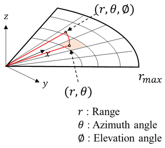
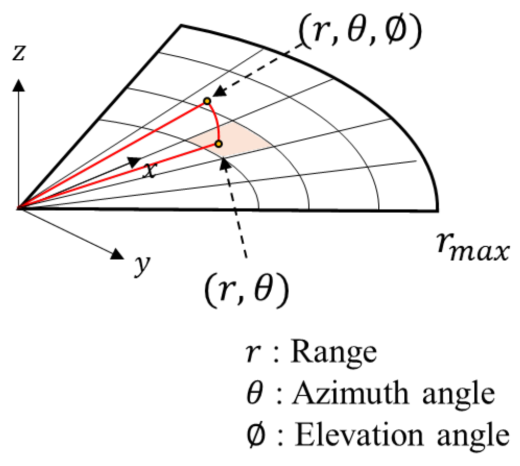
The range–azimuth projection is illustrated in Figure 1.

Figure 1. Projection of a three-dimensional point represented by range r, azimuth $\theta$, and elevation $\varphi$ onto a range–azimuth acoustic image. The elevation coordinate is not retained explicitly.

A three-dimensional point is represented by $(r,\theta ,\varphi )$, whereas an acoustic-image pixel is indexed only by $(r,\theta )$. The measured intensity can be modeled as the accumulated contribution over the vertical field of view [12]:

$$I_a(r,\theta )={\int }_{{\varphi }_{\min }}^{{\varphi }_{\max }}\beta \left(\varphi \right)V_{\mathrm{s}}(r,\theta ,\varphi )D_{\mathrm{s}}(r,\theta ,\varphi )d\varphi ,$$

(1)

where $\beta \left(\varphi \right)$ denotes the vertical beam pattern, $V_{\mathrm{s}}$ represents the target-dependent backscatter, and $D_{\mathrm{s}}$ accounts for the relationship between the incident beam and the surface normal. Consequently, echoes originating from different elevations can contribute to the same range–azimuth pixel when they share the same range and azimuth. This many-to-one projection results in elevation ambiguity and prevents a single acoustic image from uniquely determining the corresponding three-dimensional surface.

2.2. Three-Dimensional Reconstruction from Acoustic Images

Conventional reconstruction methods estimate three-dimensional geometry using multi-view feature association, reflectance-based image formation, vehicle motion, or wide-aperture observations [1,12,13,14,15,16]. The performance of these methods can depend on viewpoint diversity, sensor-pose accuracy, assumptions regarding surface scattering, and the availability of reliable acoustic features.

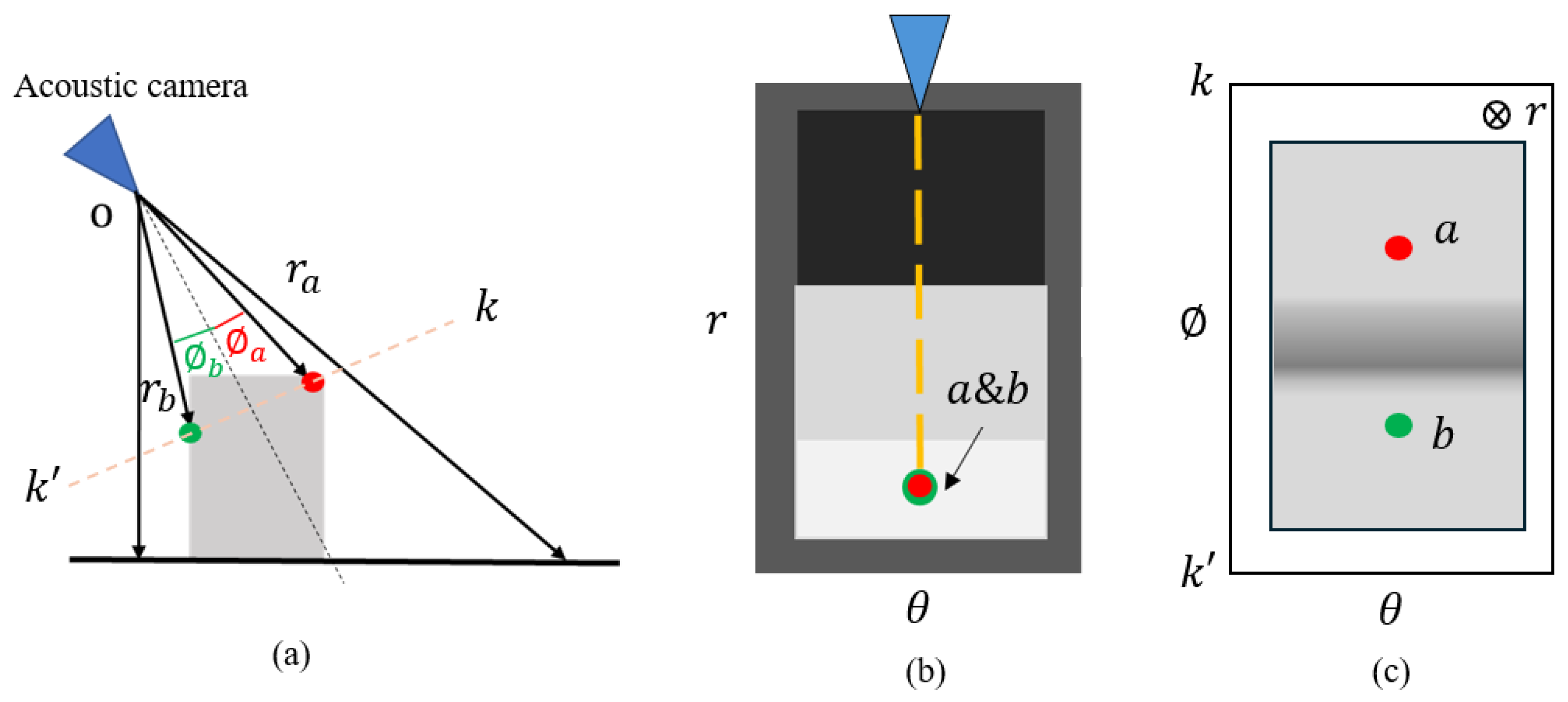
Learning-based approaches have also been developed to infer missing elevation or depth information from acoustic images. ElevateNet employs a convolutional neural network to estimate the missing spatial dimension from two-dimensional sonar images [17]. A2FNet was proposed to estimate a pseudo-front-view inverse-depth map from a single acoustic image [11]. A2FNet transforms the acoustic view into a front-view representation in which depth can be estimated with reduced elevation ambiguity, rather than directly assigning an elevation angle to each range–azimuth pixel. The network adopts an encoder–decoder architecture with U-Net-style skip connections [18]. Its input stage also employs an inverse pixel-shuffle (IPS) operation to rearrange samples along the high-resolution range dimension without discarding information. This operation corresponds to the inverse of the pixel-shuffle rearrangement introduced for efficient sub-pixel convolution [11,19].

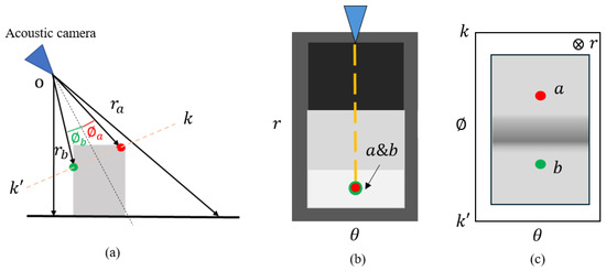
Figure 2 illustrates the relationship between the acoustic view and the pseudo-front-view inverse-depth representation.

Figure 2. Relationship between the acoustic view and the pseudo-front view: (a) acoustic imaging geometry; (b) range–azimuth view with collapsed elevation information; (c) elevation–azimuth view separating points a and b.

Learning-based multi-view approaches introduce additional geometric constraints by combining observations acquired from different viewpoints. Pseudo-front-depth multi-view stereo constructs a cost volume from a small number of FLS images [20]. Spatial Acoustic Projection integrates multi-view intensity features within a three-dimensional grid and estimates local surface distance and direction [21]. Sonar2Depth employs conditional generative adversarial networks to map acoustic observations to depth representations for three-dimensional reconstruction [22]. More recently, MV3D learns features from multiple FLS observations and predicts multi-view depth maps that are fused into a dense three-dimensional point cloud [23]. Unlike the single-view reconstruction setting considered in the present study, MV3D explicitly exploits multiple sonar viewpoints to constrain the missing elevation information.

Other approaches incorporate prior knowledge or continuous scene representations. Object-specific Bayesian inference has been used to learn the geometry of repeating subsea structures and to infer elevations for sonar returns outside the region observed by an orthogonal sonar pair [24]. More recent studies have investigated neural implicit representations and differentiable rendering for sonar-based three-dimensional reconstruction. NeuSIS combines a neural implicit surface with an acoustic volumetric renderer [25]. Differentiable space carving employs a differentiable occupancy representation to accelerate reconstruction [26]. NFFLS further improves neural-field-based FLS reconstruction using multiresolution hash encoding, frequency positional encoding, and a tailored ray-sampling strategy for efficient object-level three-dimensional reconstruction [27]. In contrast to the direct pseudo-front-view regression used by A2FNet, NFFLS represents the three-dimensional scene through a neural field and optimizes the reconstruction from sonar observations. AONeuS integrates optical images and imaging-sonar measurements within a shared neural surface framework for restricted-baseline reconstruction [28]. Related neural-rendering approaches have also addressed bathymetric reconstruction and joint optimization under sensor-pose drift [29,30].

Synthetic data generation provides another means of supporting the development and evaluation of sonar-based reconstruction methods. GPU-based sonar simulators enable the generation of synthetic acoustic observations for real-time algorithm development and evaluation [31]. More recently, ACSim incorporated recursive ray tracing, artifact modeling, and multiple forms of ground truth for learning and benchmarking [32]. Domain-translation methods can further reduce the appearance discrepancy between synthetic and real sonar images. CycleGAN provides unpaired image-to-image translation [33], and GAN-based translation has also been applied between simulated and real sonar-image domains for underwater object recognition [34].

Recent deep-learning-based frameworks have explored robust feature representation and perception across a variety of challenging sensing environments. UE-Extractor addresses ground extraction in unstructured environments using adaptive grid projection, while SAFARI-Net focuses on scale-adaptive feature refinement for infrared small-target detection [35,36]. In underwater perception, UUVDNet was developed for target detection using multibeam forward-looking sonar, whereas DAMNet applies an attention-based network to underwater biological image classification [37,38]. SWS-YOLO further investigates energy-efficient spiking neural networks for water-surface object detection [39].

Other recent studies have explored robustness to variations in imaging conditions and sensing characteristics. Meta-TIP addresses multi-dataset style adaptation for threat-image projection, while FCS-edNET applies neural-network-based restoration to magnetic particle imaging [40,41]. Although these methods address sensing modalities and perception tasks different from the single-view FLS-based three-dimensional reconstruction considered in this study, they demonstrate recent efforts to improve feature representation, robustness, and task-specific perception under challenging sensing conditions. They are therefore discussed as related learning-based approaches rather than as direct reconstruction baselines.

Despite these advances, the influence of the geometric distribution of synthetic training data on reconstruction accuracy has received comparatively limited attention. In particular, a model trained primarily on planar or brick-like geometries may exhibit degraded reconstruction accuracy when applied to curved structures such as cylinders and spheres. Therefore, this study investigates how shape-specific training datasets influence A2FNet reconstruction accuracy while maintaining the same network architecture and training procedure.

It should be noted that several recent sonar-based three-dimensional reconstruction methods operate under different sensing and reconstruction settings. Multi-view methods such as pseudo-front-depth multi-view stereo and Spatial Acoustic Projection require multiple FLS observations, whereas other approaches employ neural implicit representations, differentiable rendering, or multimodal sensing. Direct quantitative comparison with these methods is therefore not straightforward under the single-view pseudo-front-view regression setting considered in this study.

These studies address different aspects of underwater perception and sonar-based three-dimensional reconstruction. DeepAquaEnhance focuses on restoring degraded optical underwater images, whereas ElevateNet and A2FNet estimate missing geometric information from sonar images. MV3D exploits multiple FLS viewpoints, and NFFLS represents the scene using neural fields. In contrast, the objective of the present study is not to introduce a new reconstruction or image-translation architecture. The A2FNet architecture and CycleGAN-based appearance-translation procedure are intentionally fixed to investigate how the geometric composition of synthetic training data affects reconstruction accuracy under a single-view setting.

3. Materials and Methods

3.1. Overall Framework

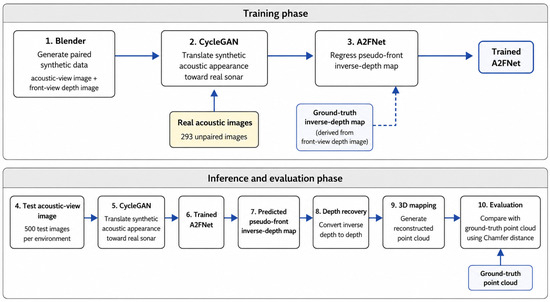
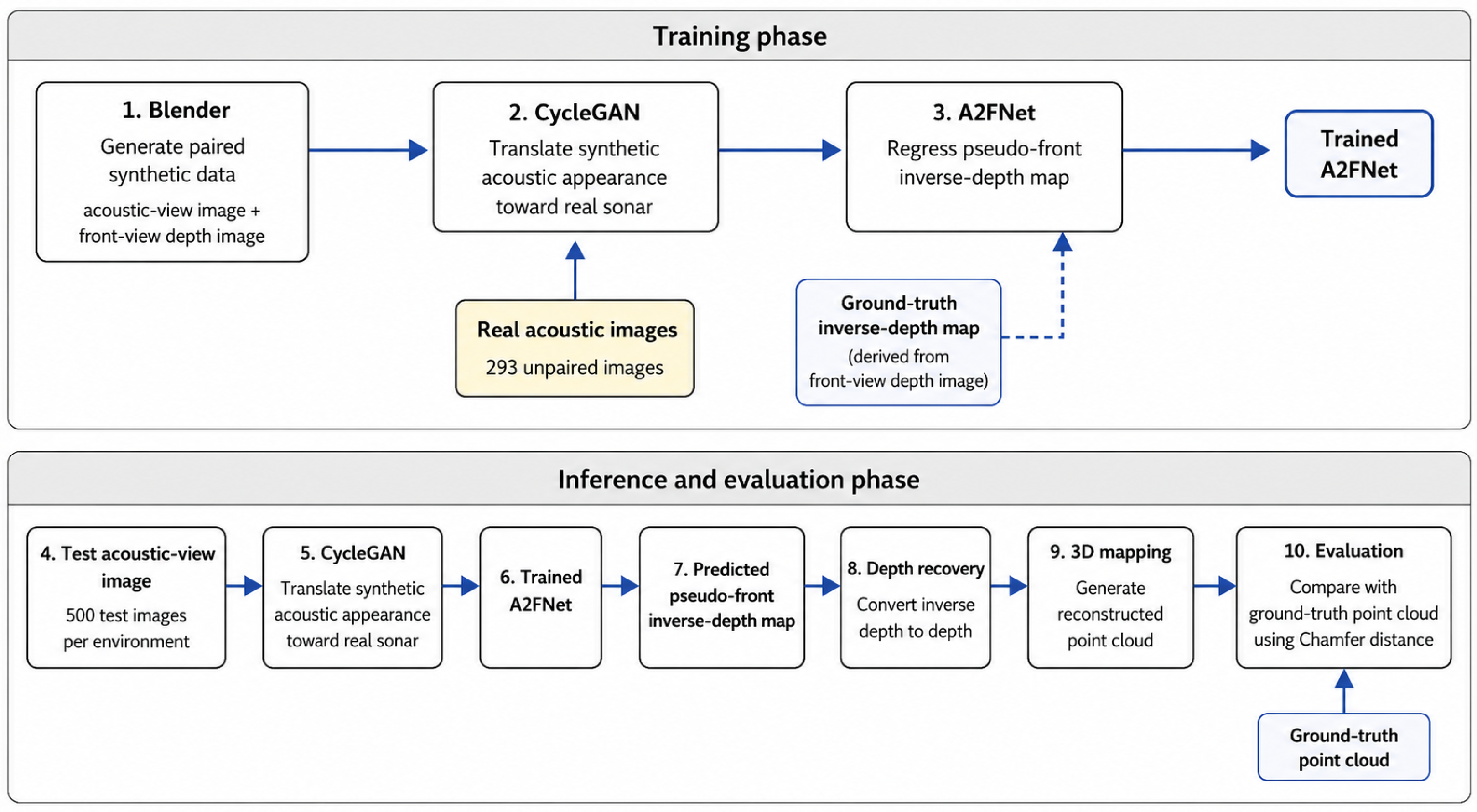
Figure 3 illustrates the overall workflow of the proposed framework. First, Blender (version 2.90; Blender Foundation, Amsterdam, The Netherlands) is used to generate paired acoustic-view images and front-view depth images [42]. Each synthetic acoustic-view image is then translated toward the real-sonar image domain using CycleGAN, while the corresponding front-view depth image is retained without modification. The front-view depth image is converted into an inverse-depth representation and used as the ground-truth target for A2FNet. A2FNet is trained to estimate a pseudo-front-view inverse-depth map from the translated acoustic-view image.

Figure 3. Overall workflow of the proposed framework. Synthetic acoustic-view images are translated using the trained synthetic-to-real CycleGAN generator before being provided to A2FNet during both training and inference.

During inference, each synthetic acoustic-view test image is first translated using the trained synthetic-to-real CycleGAN generator and then provided to the trained A2FNet. The predicted inverse-depth map is converted back into a depth representation and subsequently used to reconstruct a three-dimensional point cloud. The reconstructed point cloud is compared with the corresponding simulator-generated ground-truth point cloud using CD.

3.2. Synthetic Dataset Generation

Obtaining large acoustic-image datasets with accurately registered geometric ground truth is costly and technically difficult in underwater environments. Therefore, paired synthetic data were generated using Blender, a three-dimensional computer graphics application.

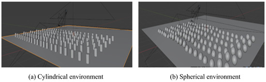
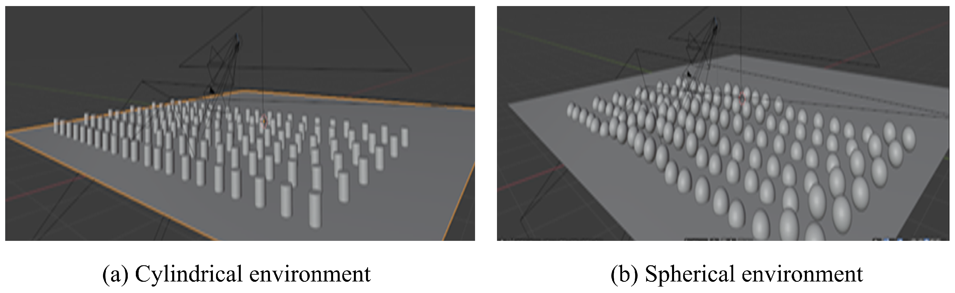
As shown in Figure 4, two virtual environments were constructed using multiple cylinders or spheres arranged on a ground plane. The cylinder-specific scene contained 126 cylinders arranged in a structured $6\times 21$ configuration. Each cylinder had a diameter of 0.2000 and a height of 0.2500 in the common simulator coordinate system. The sphere-specific scene contained 120 spheres arranged in a structured $6\times 20$ configuration. Each sphere had a diameter of 0.3241.

Figure 4. Synthetic environments constructed in Blender for dataset generation: (a) the cylinder-specific scene and (b) the sphere-specific scene. The objects were placed in structured arrangements on a ground plane.

For each camera pose, two geometrically corresponding images were generated, namely an acoustic-view image and a front-view depth image. The acoustic-view image represents a range–azimuth observation from a forward-looking acoustic camera in which elevation-dependent information is collapsed. In contrast, the front-view depth image retains the elevation-dependent geometry of the observed objects. The synthetic acoustic-view images served as the source images for CycleGAN translation, and the translated images were subsequently used as inputs to A2FNet. Valid depth values in the corresponding front-view images were converted into inverse-depth values and used as the ground-truth targets.

For each object-specific scene, 4500 camera poses were generated using a fixed random seed of 0. In the common simulator coordinate system, the camera x coordinate was sampled approximately from $-1.2$ to $0.8$, and the y coordinate was sampled from $-4.0$ to $4.0$. The camera height was fixed at $z=1.5$, and the Blender XYZ Euler angles were fixed at $({51}^{\circ },0^{\circ },{90}^{\circ })$. One acoustic-view image and one front-view depth image were generated for each camera pose, resulting in 4500 paired observations for each basic Blender scene.

Of the 4500 image pairs generated for each basic Blender scene, 4000 were assigned to the A2FNet training set and were used during training. The remaining 500 image pairs were reserved as the test set and were used only for inference and reconstruction-performance evaluation.

The mixed training dataset was constructed using 2000 images from the cylinder training set and 2000 images from the sphere training set. Separately, 500 image pairs were generated for each HoloOcean-derived environment and reserved as its test set. These images were used only for inference and reconstruction-performance evaluation.

Four A2FNet training datasets were prepared, as summarized in Table 1. The cylinder-specific model ${\mathrm{Model}}_{\mathrm{c}}$ was trained using 4000 cylinder images, and the sphere-specific model ${\mathrm{Model}}_{\mathrm{s}}$ was trained using 4000 sphere images. The mixed model ${\mathrm{Model}}_{\mathrm{cs}}$ was trained using 2000 cylinder images and 2000 sphere images. For comparison, ${\mathrm{Model}}_p$ was included as a reference model representing the training-data configuration used in the previous A2FNet study [11]. Its training data were generated primarily from brick-like objects placed with varying poses, and therefore differed substantially in geometric composition from the cylinder-specific and sphere-specific datasets introduced in the present study. ${\mathrm{Model}}_p$ used the same A2FNet architecture and was evaluated on the same test sets as the other models. Additional geometric, camera, and image-generation parameters are provided in Appendix A.3.

Table 1. A2FNet training datasets and model identifiers. ${\mathrm{Model}}_p$ denotes the reference model based on the previous-study training dataset.

Model	Cylinder Images	Sphere Images	Previous-Study Images
${\mathrm{Model}}_{\mathrm{c}}$	4000	–	–
${\mathrm{Model}}_{\mathrm{s}}$	–	4000	–
${\mathrm{Model}}_{\mathrm{cs}}$	2000	2000	–
${\mathrm{Model}}_{\mathrm{p}}$	–	–	4000

3.3. CycleGAN-Based Appearance Translation

Although Blender provides accurately paired acoustic-view images and front-view depth images, the appearance of the generated acoustic images differs from that of images acquired by real acoustic cameras. CycleGAN was therefore employed to translate the synthetic acoustic images toward the real acoustic-image domain without requiring paired synthetic and real images [33].

The standard CycleGAN architecture and objective function proposed by Zhu et al. [33] were used. The training conditions followed those adopted in the original A2FNet study [11]. Because pretrained CycleGAN weights from the original A2FNet study were not publicly available, the CycleGAN model used in the present study was independently trained in our experimental environment following the previously reported training configuration. No new CycleGAN architecture or training strategy was introduced in the present study.

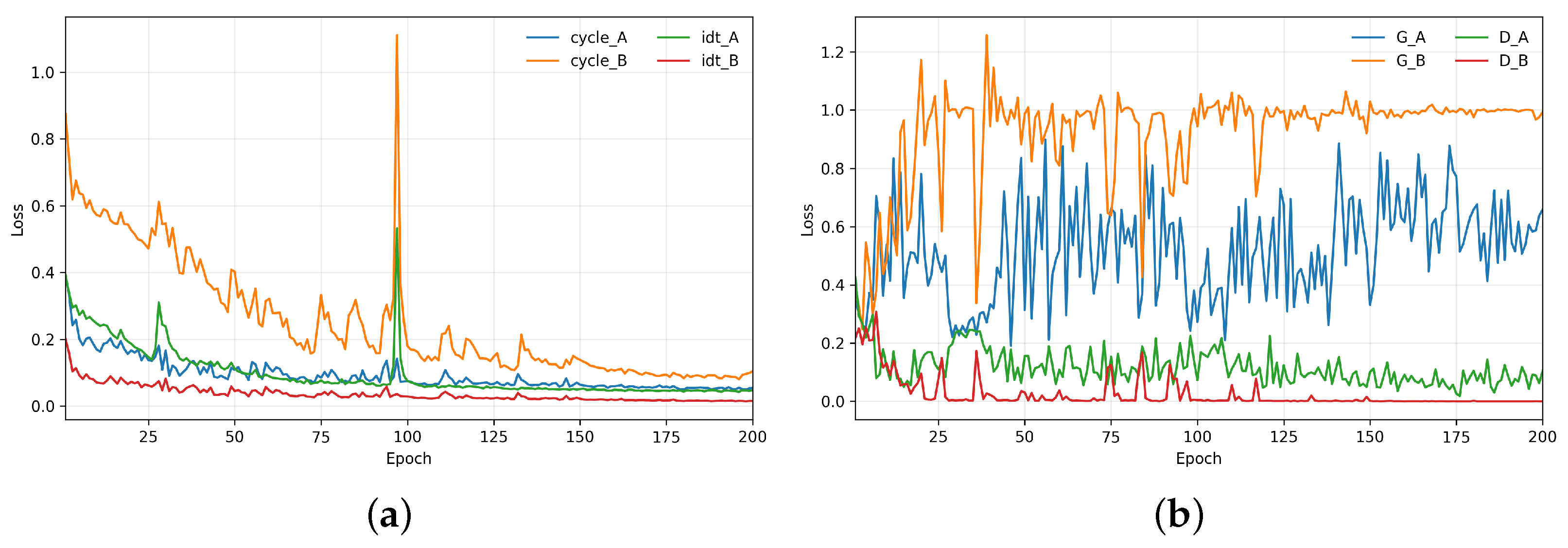
The unpaired domain-translation dataset consisted of 239 synthetic acoustic images and 293 real acoustic-camera images. CycleGAN was trained for 200 epochs with a batch size of 1 and an initial learning rate of 0.0002. The learning rate was maintained for the first 100 epochs and then linearly decayed toward zero over the remaining 100 epochs. The corresponding training loss curves are provided in Appendix B.

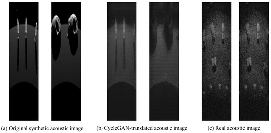
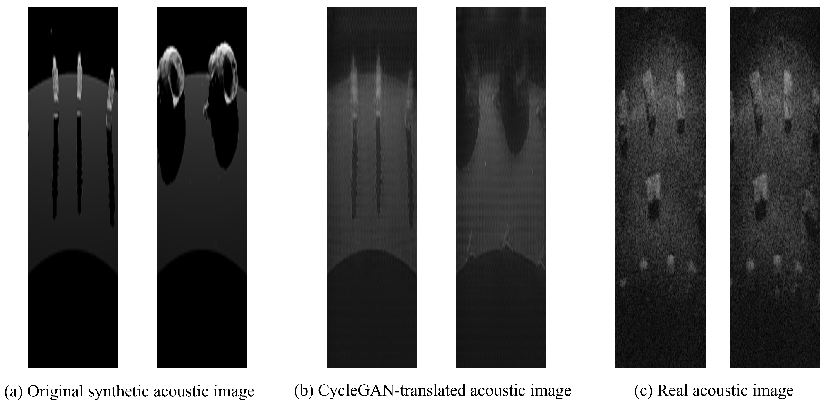
Figure 5 presents representative synthetic acoustic images before translation, the corresponding CycleGAN-translated images, and unpaired real acoustic-camera images from the target domain. The examples qualitatively illustrate the appearance change introduced by the synthetic-to-real translation. In particular, the translated images exhibit intensity and texture characteristics that are visually closer to those of the real acoustic-image domain than the original synthetic images.

Figure 5. Representative examples of acoustic-image appearance translation. The columns show (a) synthetic acoustic-view images before translation, (b) the corresponding CycleGAN-translated images, and (c) representative real acoustic-camera images from the target domain.

After training, the synthetic-to-real generator was applied to the synthetic acoustic-view images used for both A2FNet training and inference. The corresponding front-view depth images were retained without modification, thereby preserving the original sample-level pairing between each acoustic-view image and its corresponding depth target.

The CycleGAN model was trained once before the A2FNet experiments, and the same trained synthetic-to-real generator was used throughout the subsequent experiments. In particular, CycleGAN was not retrained when the cylinder training-scene configuration was revised. The same generator was applied to both the original and revised synthetic datasets. Therefore, the before-and-after comparison of the cylinder training-scene revision was conducted without changing the CycleGAN model.

3.4. A2FNet Training

A separate A2FNet model was trained for each dataset listed in Table 1. The network input was a CycleGAN-translated acoustic-view image. The corresponding front-view depth image generated in Blender was converted into a pseudo-front-view inverse-depth representation and used as the regression target.

The network architecture, loss function, and basic optimization settings were based on the publicly available A2FNet implementation [11]. The network parameters were optimized using Adam with a fixed learning rate of 0.001. The training batch size was 8, and each model was trained for 200 epochs. The checkpoint obtained at the end of the 200th epoch was used for all reported evaluations.

The 4000 images assigned to each training set were shuffled and processed once per epoch. Because the number of training images was exactly divisible by the batch size, all training samples were used in every epoch, resulting in 500 parameter-update steps per epoch. The mean absolute error between the predicted and ground-truth pseudo-front-view inverse-depth maps was used as the training loss. During training, a joint horizontal flip was applied to the acoustic-view input and its corresponding target with a probability of 0.5.

The 500 Blender test images and the separately generated 500 HoloOcean-derived test images for each environment were used exclusively for inference and reconstruction-performance evaluation. None of the test images were used for parameter optimization, hyperparameter tuning, learning-rate control, or model selection. Further implementation details are provided in Appendix A.1.

The cylinder-specific model ${\mathrm{Model}}_{\mathrm{c}}$, sphere-specific model ${\mathrm{Model}}_{\mathrm{s}}$, mixed model ${\mathrm{Model}}_{\mathrm{cs}}$, and previous-data model ${\mathrm{Model}}_{\mathrm{p}}$ used the same A2FNet architecture and optimization settings.

3.5. Point-Cloud Reconstruction

During inference, a CycleGAN-translated acoustic-view image is provided to the trained A2FNet to estimate a pseudo-front-view inverse-depth map with a resolution of $32\times 128$. The estimated inverse-depth map is subsequently converted into a three-dimensional point cloud using the same geometric conversion as that applied to the ground-truth inverse-depth map.

First, each inverse-depth value ${\widehat{D}}^{-1}(m,j)$ is converted to the corresponding depth as

$$r(m,j)={\displaystyle \frac{1}{{\widehat{D}}^{-1}(m,j)}},$$

(2)

where m and j denote the vertical and horizontal pixel indices, respectively. The recovered depth is then converted to a discrete range-bin index according to

$$k(m,j)=⌊{\displaystyle \frac{r(m,j)-r_{\min }}{\Delta r}}⌋,$$

(3)

where $r_{\min }=2.0$ and $\Delta r=0.003$ in the point-cloud conversion procedure. Range-bin indices outside the range of 0–511 are treated as invalid, and only positive valid range-bin indices are retained for point-cloud generation. For each valid range bin, the radial distance is reconstructed as

$$r_k=r_{\min }+k\Delta r.$$

(4)

The vertical and horizontal pixel positions in the pseudo-front view are then mapped to elevation and azimuth angles, respectively. For the $32\times 128$ representation used in this study, the elevation angle is calculated as

$${\varphi }_m=-7^{\circ }+{\displaystyle \frac{m}{32}}\times {14}^{\circ },$$

(5)

and the azimuth angle is calculated as

$${\theta }_j=-{16}^{\circ }+{\displaystyle \frac{j}{128}}\times {32}^{\circ }.$$

(6)

These mappings correspond to nominal elevation and azimuth angular spans of ${14}^{\circ }$ and ${32}^{\circ }$, respectively.

Finally, each valid sample $(r_k,{\theta }_j,{\varphi }_m)$ is converted from spherical to Cartesian coordinates according to

$$\begin{array}{cc}\hfill x& =r_k\cos {\theta }_j\cos {\varphi }_m,\hfill \\ \hfill y& =r_k\sin {\theta }_j\cos {\varphi }_m,\hfill \\ \hfill z& =r_k\sin {\varphi }_m.\hfill \end{array}$$

(7)

This conversion is applied to all valid pixels to generate the reconstructed point cloud. The same procedure is applied to the corresponding ground-truth inverse-depth map, ensuring that the predicted and ground-truth point clouds are represented using the same coordinate definition. The resulting Cartesian coordinates are saved in ASC format.

The reconstructed point cloud is quantitatively compared with the corresponding simulator-generated ground-truth point cloud using symmetric CD. A lower CD value indicates greater geometric agreement between the two point clouds, and the detailed definition of the evaluation metric is provided in Section 4.1. For visualization, the ASC point clouds are imported into MeshLab (version 2023.12; Visual Computing Lab, ISTI-CNR, Pisa, Italy), where surface reconstruction is applied to facilitate visual inspection. This visualization step is independent of the quantitative evaluation performed directly on the point-cloud coordinates.

3.6. Evaluation Environments

Four evaluation environments were prepared. These consisted of (I) cylinders arranged in a structured Blender environment, (II) spheres arranged in a structured Blender environment, (III) a cylindrical environment derived from the HoloOcean dam environment, and (IV) a spherical environment derived from HoloOcean.

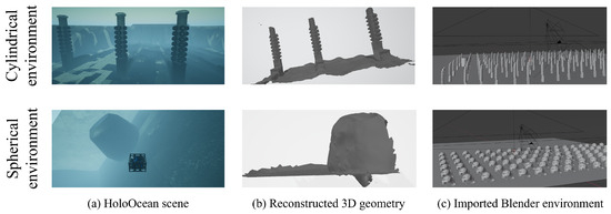
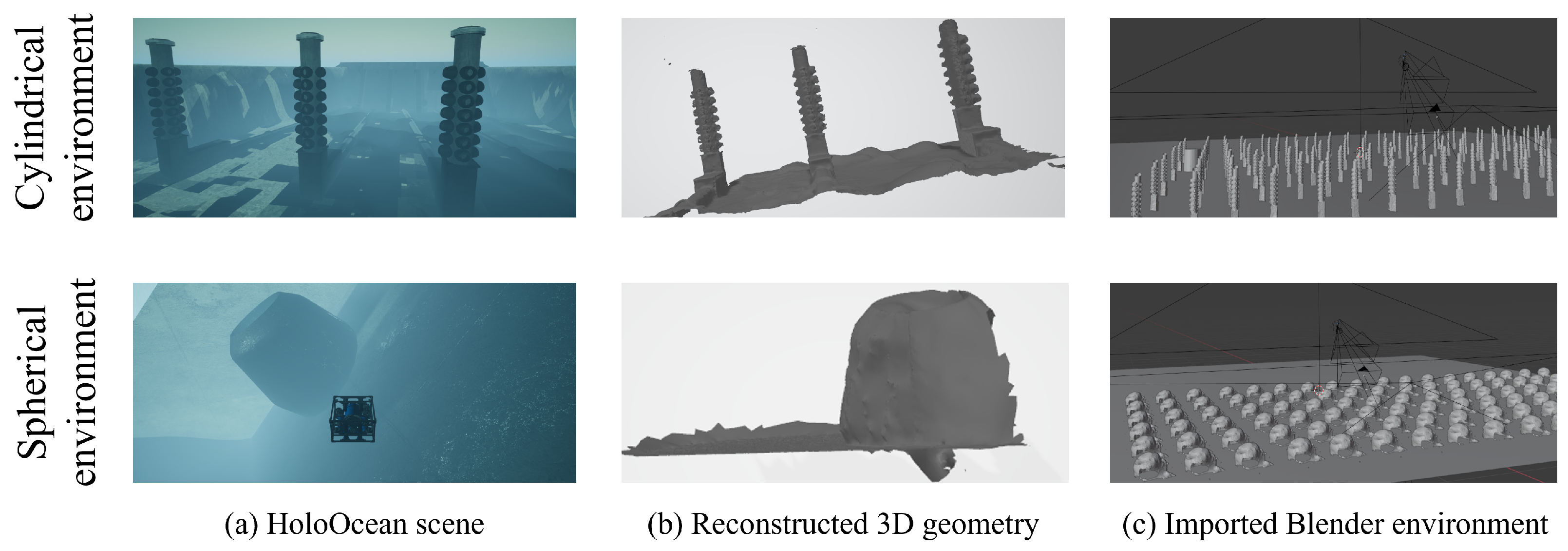
For the HoloOcean-derived environments, images of the virtual marine scenes were first obtained using HoloOcean, an underwater robotics simulator designed for marine robotics applications [2]. As shown in Figure 6, the corresponding three-dimensional geometries were reconstructed using Agisoft Metashape Professional (version 2.0.3; Agisoft LLC, St. Petersburg, Russia) [43] and subsequently imported into Blender. Acoustic-view images and front-view depth images were then generated from the imported geometries using the same image-generation procedure as that used for the basic Blender environments.

Figure 6. Generation of the HoloOcean-derived evaluation environments. The upper and lower rows show the cylindrical and spherical environments, respectively. The columns show (a) the original HoloOcean scenes, (b) the three-dimensional geometries reconstructed using Agisoft Metashape, and (c) the reconstructed geometries imported into Blender.

The HoloOcean-derived environments contain more irregular object geometries and more complex scene structures than the structured Blender environments. All four evaluation environments are simulation-derived. Therefore, the quantitative results in this study evaluate reconstruction performance within simulation-based domains and do not establish generalization to field-acquired FLS measurements.

For each evaluation environment, 500 test-image pairs were prepared and used exclusively for inference and reconstruction-performance evaluation. For the cylindrical environments, ${\mathrm{Model}}_{\mathrm{c}}$, ${\mathrm{Model}}_{\mathrm{cs}}$, and ${\mathrm{Model}}_{\mathrm{p}}$ were evaluated; for the spherical environments, ${\mathrm{Model}}_{\mathrm{s}}$, ${\mathrm{Model}}_{\mathrm{cs}}$, and ${\mathrm{Model}}_{\mathrm{p}}$ were evaluated.

4. Results

4.1. Evaluation Metric

Reconstruction accuracy was evaluated using symmetric CD, which measures the geometric discrepancy between two point sets [11,44]. Let ${\mathcal{S}}_1$ and ${\mathcal{S}}_2$ denote the predicted and ground-truth point sets, respectively. The CD used in this study is defined as

$$\begin{array}{cc}\hfill \mathrm{CD}({\mathcal{S}}_1,{\mathcal{S}}_2)=& {\displaystyle \frac{\lambda }{|{\mathcal{S}}_1|}}\sum _{\mathbf{x}\in {\mathcal{S}}_1}\underset{\mathbf{y}\in {\mathcal{S}}_2}{\min }{∥\mathbf{x}-\mathbf{y}∥}_2^2\hfill \\ & +{\displaystyle \frac{\lambda }{|{\mathcal{S}}_2|}}\sum _{\mathbf{y}\in {\mathcal{S}}_2}\underset{\mathbf{x}\in {\mathcal{S}}_1}{\min }{∥\mathbf{y}-\mathbf{x}∥}_2^2,\hfill \end{array}$$

(8)

where $\lambda$ is a scaling factor set to 500 following the evaluation protocol of the original A2FNet study [11]. This scaling is used to maintain consistency with the original evaluation protocol and changes only the numerical magnitude of the metric without affecting the relative ranking of the evaluated models. The corresponding unscaled CD is obtained by setting $\lambda =1$, or equivalently by dividing the reported CD values by 500. The unscaled results are provided in Appendix C.

All point coordinates are represented in the common simulator coordinate system used for synthetic data generation. Accordingly, the CD values are interpreted as squared geometric discrepancies in this coordinate system rather than as errors expressed in a calibrated physical unit. No additional normalization or scale adjustment was applied to either the predicted or ground-truth point clouds before CD calculation. A lower CD value indicates greater geometric agreement between the predicted and ground-truth point clouds.

4.2. Representative Reconstruction Results

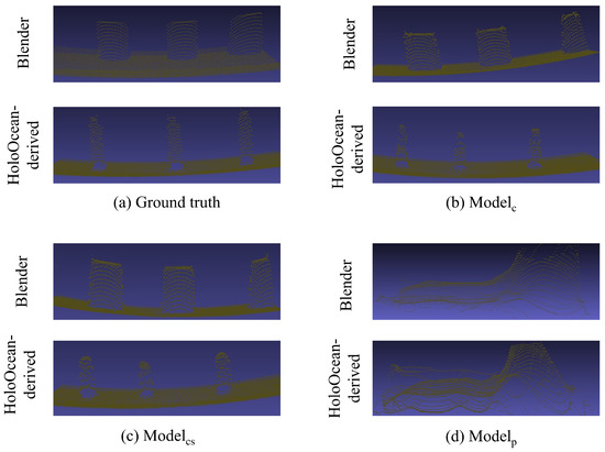
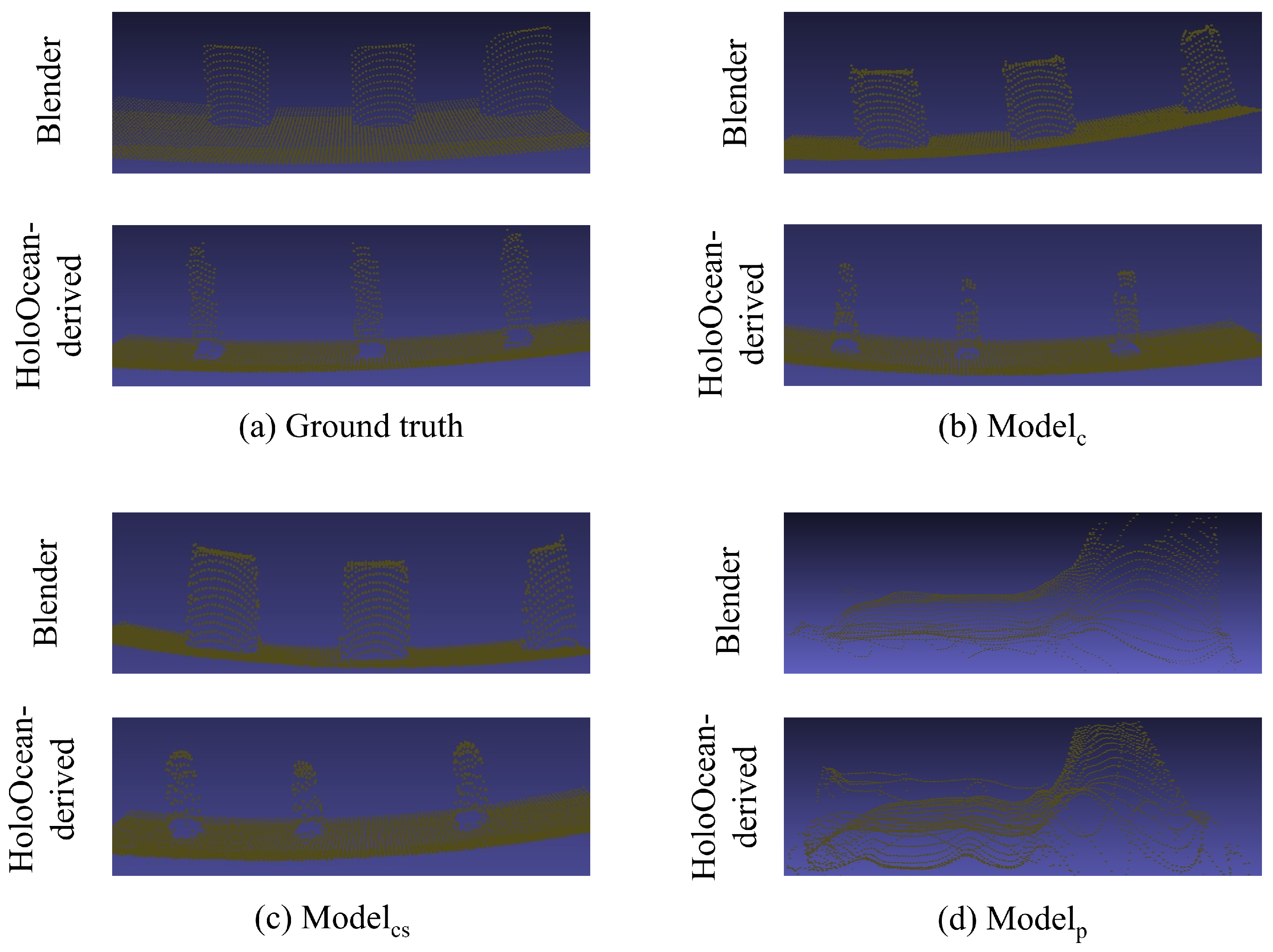
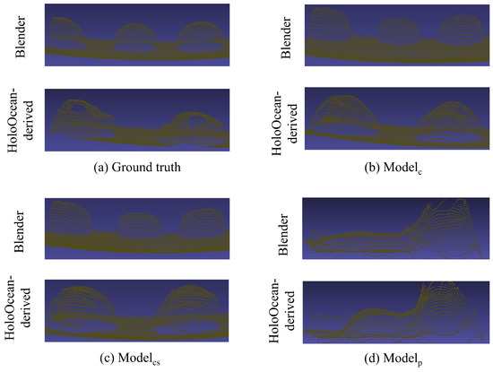
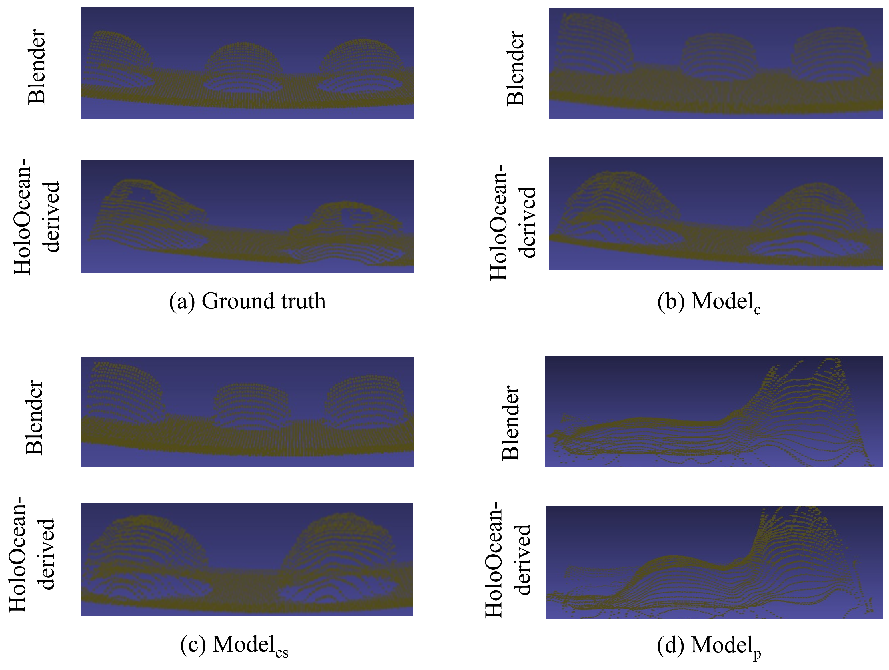
For each test image, the CD values obtained using the three evaluated models were averaged. The representative sample was selected as the test image whose average CD was closest to the median of these 500 image-wise average values. The same test-image index was used for all models shown in Figure 7 and Figure 8.

Figure 7. Representative 3D mapping results for the cylindrical environments. The upper row shows the results for the Blender environment, and the lower row shows the results for the HoloOcean-derived environment. From left to right, the columns correspond to the ground truth, the cylinder-specific model ${\mathrm{Model}}_{\mathrm{c}}$, the mixed model ${\mathrm{Model}}_{\mathrm{cs}}$, and the previous-data model ${\mathrm{Model}}_{\mathrm{p}}$.

Figure 8. Representative 3D mapping results for the spherical environments. The upper row shows the results for the Blender environment, whereas the lower row shows the results for the HoloOcean-derived environment. From left to right, the columns correspond to the ground truth, the sphere-specific model ${\mathrm{Model}}_{\mathrm{s}}$, the mixed model ${\mathrm{Model}}_{\mathrm{cs}}$, and the previous-data model ${\mathrm{Model}}_{\mathrm{p}}$.

Table 2 summarizes the CD values corresponding to the representative point-cloud reconstructions shown in Figure 7 and Figure 8. For these representative samples, both the specialized and mixed models produce substantially lower CD values than the previous-data model in all four evaluation environments.

Table 2. Representative Chamfer distance (CD) results for the four evaluation environments.

Environment	Specialized Model	Mixed Model	Previous-Data Model	Best Reduction vs. Previous-Data Model (%)
Blender cylinders	1.1520 (${\mathrm{Model}}_{\mathrm{c}}$)	1.1845	78.7676	98.54%
HoloOcean-derived cylinders	1.0316 (${\mathrm{Model}}_{\mathrm{c}}$)	0.1116	74.7003	99.85%
Blender spheres	4.4362 (${\mathrm{Model}}_{\mathrm{s}}$)	4.3707	75.7816	94.23%
HoloOcean-derived spheres	1.1803 (${\mathrm{Model}}_{\mathrm{s}}$)	1.1261	103.8565	98.92%

For the Blender cylinder environment, the CD value obtained using ${\mathrm{Model}}_{\mathrm{c}}$ is 1.1520, compared with 78.7676 for ${\mathrm{Model}}_{\mathrm{p}}$. In the HoloOcean-derived cylinder environment, ${\mathrm{Model}}_{\mathrm{cs}}$ achieves the lowest value of 0.1116, whereas ${\mathrm{Model}}_{\mathrm{p}}$ produces a value of 74.7003.

For the Blender sphere environment, ${\mathrm{Model}}_{\mathrm{s}}$ and ${\mathrm{Model}}_{\mathrm{cs}}$ produce similar values of 4.4362 and 4.3707, respectively, compared with 75.7816 for ${\mathrm{Model}}_{\mathrm{p}}$. For the HoloOcean-derived sphere environment, the corresponding values are 1.1803, 1.1261, and 103.8565.

As shown in Figure 7, the cylinder-specific and mixed models produce similar reconstructions in the basic Blender environment. In the HoloOcean-derived environment, both models produce target locations and ground-plane structures that are in closer agreement with the ground truth than those produced by the previous-data model. The reconstructed cylinders remain shorter than those in the ground truth. This result suggests a geometry mismatch between the short, thick cylinders used for training and the taller, narrower structures in the HoloOcean-derived test environment.

Figure 8 shows that both the sphere-specific and mixed models recover the locations and approximate shapes of the spherical targets. In the basic Blender environment, some of the reconstructed spheres exhibit flattened or truncated upper surfaces. In the HoloOcean-derived environment, the ground-truth objects contain irregular surface structures, whereas the reconstructed objects are smoother and more rounded. This difference suggests that the reconstructed shapes are biased toward the smooth spherical geometries represented in the Blender training dataset.

4.3. Mean CD over 500 Test Images

Table 3 summarizes the mean CD over 500 test images for each environment and model. Among the models trained on the original datasets, ${\mathrm{Model}}_{\mathrm{cs}}$ achieves the lowest mean CD in the Blender and HoloOcean-derived cylinder environments (7.7329 and 1.8341), reducing the values obtained with ${\mathrm{Model}}_{\mathrm{p}}$ by 91.16% and 97.63%, respectively. In the corresponding sphere environments, ${\mathrm{Model}}_{\mathrm{s}}$ achieves the lowest values (4.6689 and 5.2430), representing reductions of 94.72% and 94.23%, respectively. Thus, although the mixed dataset enables one model to be applied to both object categories, it does not consistently outperform geometry-specific training.

Table 3. Mean CD over 500 test images obtained using models trained on the original synthetic datasets. The symbol “–” indicates that the corresponding model was not evaluated for that object category.

Environment	${\mathbf{Model}}_{\mathbf{c}}$	${\mathbf{Model}}_{\mathbf{s}}$	${\mathbf{Model}}_{\mathbf{cs}}$	${\mathbf{Model}}_{\mathbf{p}}$
Blender cylinders	17.6459	–	7.7329	87.4441
HoloOcean-derived cylinders	2.4071	–	1.8341	77.3280
Blender spheres	–	4.6689	8.9504	88.4414
HoloOcean-derived spheres	–	5.2430	10.4124	90.8582

4.4. Large-Error Analysis and Training-Scene Revision

To identify large-error cases objectively, the per-image CD values in the original Blender cylinder test set were analyzed for ${\mathrm{Model}}_{\mathrm{c}}$ and ${\mathrm{Model}}_{\mathrm{cs}}$. For each model, test images with CD values equal to or greater than the model-specific 95th percentile were classified as large-error cases. Each threshold selected 25 of the 500 test images, and the selected test-image indices were identical for the two models. The per-image CD rankings were also strongly correlated over all 500 test images. These results indicate that the large reconstruction errors were associated with particular input observations rather than being specific to one trained model.

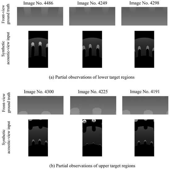
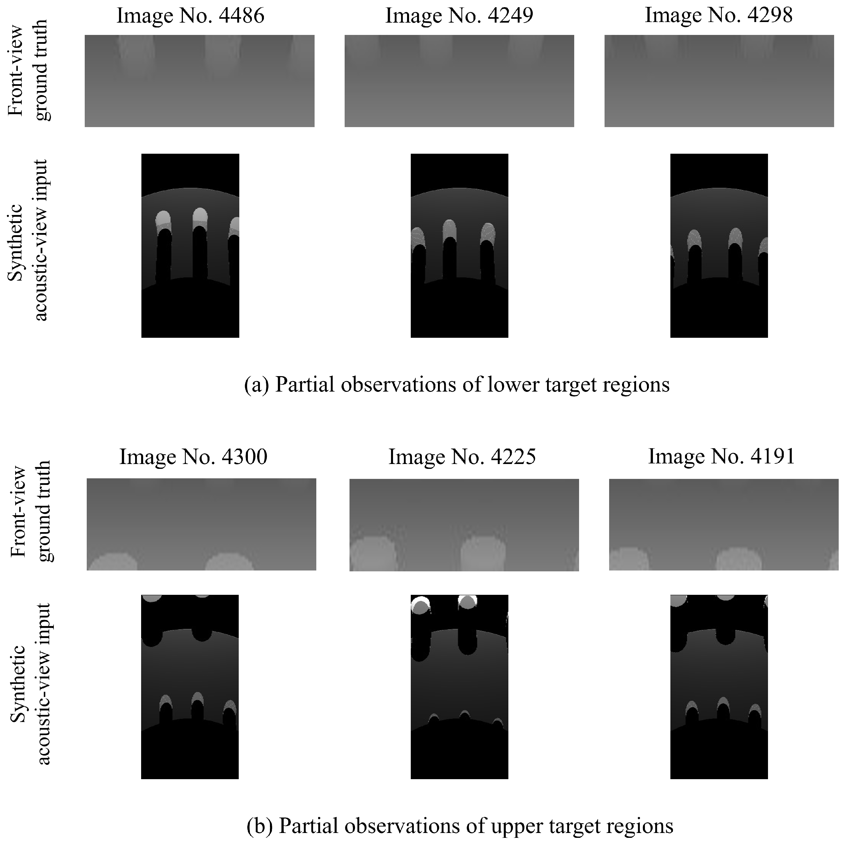
Visual inspection of the shared large-error cases revealed recurring observations in which the cylindrical targets are only partially contained in the camera field of view. Figure 9 presents representative examples selected from these 25 shared large-error cases. The untranslated synthetic acoustic-view images are shown to directly visualize the target coverage and geometric truncation in the original simulated observations. The actual A2FNet inputs were obtained by applying the trained CycleGAN generator to these images. As shown in Figure 9, some front-view ground-truth images and the corresponding untranslated synthetic acoustic-view images contain only the upper or lower regions of the cylindrical targets. These incomplete target profiles are associated with large CD values and may provide fewer geometric cues for pseudo-front-view inverse-depth estimation. The corresponding untranslated synthetic acoustic-view images also exhibit weak or irregular grayscale responses around partially visible objects. These observations suggest that insufficient target coverage may have contributed to ambiguity in the predicted pseudo-front-view inverse-depth maps.

Figure 9. Representative examples selected from the 25 large-error images shared by ${\mathrm{Model}}_{\mathrm{c}}$ and ${\mathrm{Model}}_{\mathrm{cs}}$ in the original Blender cylinder test set. The figure shows paired front-view ground-truth images and untranslated synthetic acoustic-view images associated with large CD values. The upper group shows examples in which only the lower regions of the cylindrical targets are contained in the observation, whereas the lower group shows examples in which only the upper regions are contained. Within each group, the first row presents the front-view ground-truth images, and the second row presents the corresponding untranslated synthetic acoustic-view images.

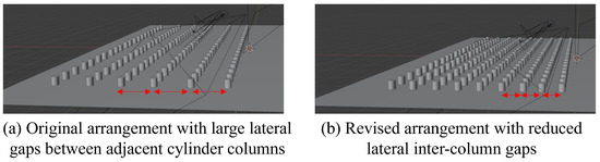
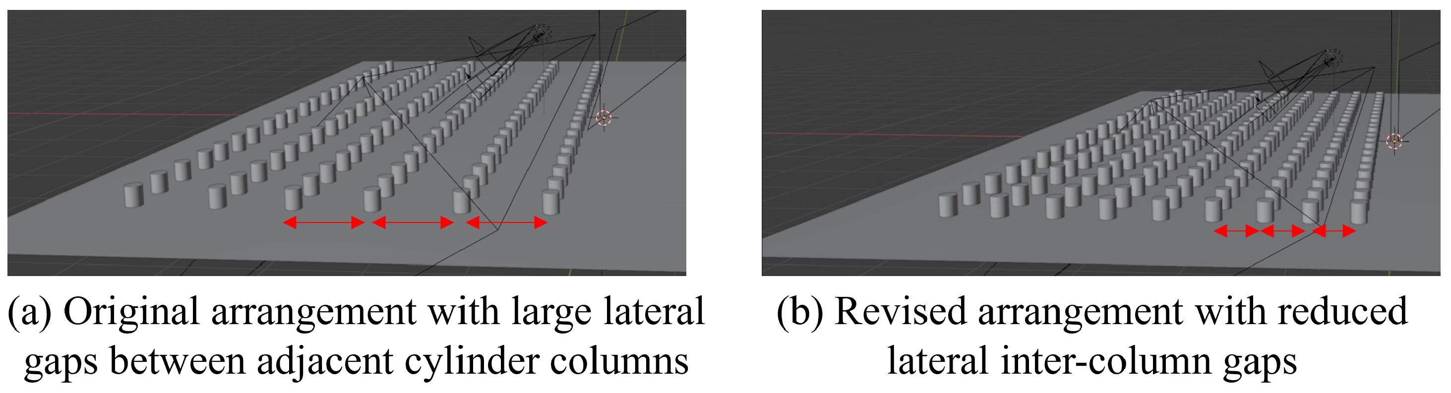
This observation motivated revision of the cylinder training-scene configuration. In the original scene, 126 cylinders were arranged in a structured $6\times 21$ configuration. The mean lateral surface gap between adjacent columns was 0.8331. The revised configuration increased the number of columns from six to nine while retaining 21 cylinders per column and the same cylinder dimensions. As shown in Figure 10, the mean lateral surface gap was reduced to 0.4156, corresponding to a reduction of approximately 50.1%.

Figure 10. Revision of the cylinder arrangement used for synthetic training-data generation. (a) Original $6\times 21$ arrangement with lateral surface-to-surface gaps ranging from 0.7626 to 0.8875 and a mean gap of 0.8331. (b) Revised $9\times 21$ arrangement with lateral gaps ranging from 0.3337 to 0.4770 and a mean gap of 0.4156. The cylinder diameter and height were maintained at 0.2000 and 0.2500, respectively.

Because the revision increased the number of cylinder columns while reducing the inter-column spacing, it simultaneously changed the total number of objects, object density, and target occupancy under the fixed camera configuration. Therefore, this revision should be regarded as a composite modification of the training-scene configuration. The following experiment evaluates the overall effect of this revised configuration and does not isolate the contribution of any individual geometric factor.

Table 4 summarizes the per-image CD statistics before and after revision of the cylinder component of the training datasets. Each statistic was calculated from the same 500 test images. The cylinder training dataset was regenerated using the revised arrangement. The same camera poses and pretrained synthetic-to-real CycleGAN generator were used for the original and revised datasets. ${\mathrm{Model}}_{\mathrm{c}}$ was retrained using all 4000 revised cylinder images. For ${\mathrm{Model}}_{\mathrm{cs}}$, the mixed dataset consisted of 2000 revised cylinder images and the same 2000 sphere images used in the original mixed dataset. The retrained models were evaluated using the same test sets as before the revision. The sphere-specific ${\mathrm{Model}}_{\mathrm{s}}$ was not retrained and was retained as an unchanged reference for the spherical environments.

Table 4. Per-image CD statistics before and after revision of the cylinder component of the training datasets. The sphere-specific model is included as an unchanged reference. Each statistic was calculated from 500 test images.

Environment	Model	Dataset Status	Mean	Median	95th Percentile	Maximum
Blender cylinders	${\mathrm{Model}}_{\mathrm{c}}$	Original	17.6459	3.4371	143.7272	465.5735
		Revised	3.1345	3.2516	5.1560	8.7512
Blender cylinders	${\mathrm{Model}}_{\mathrm{cs}}$	Original	7.7329	3.3466	42.4881	113.0430
		Revised	3.0721	3.0014	5.7730	7.8418
Blender spheres	${\mathrm{Model}}_{\mathrm{s}}$	Unchanged reference	4.6689	4.2289	9.5013	11.9816
Blender spheres	${\mathrm{Model}}_{\mathrm{cs}}$	Original	8.9504	4.3803	46.8171	105.5375
		Revised	4.3692	4.0907	9.0796	11.9897
HoloOcean-derived cylinders	${\mathrm{Model}}_{\mathrm{c}}$	Original	2.4071	0.9684	2.9792	165.2562
		Revised	1.0336	0.6781	2.6681	5.3346
HoloOcean-derived cylinders	${\mathrm{Model}}_{\mathrm{cs}}$	Original	1.8341	1.1152	3.4246	46.0096
		Revised	1.2328	0.9666	3.1304	6.9811
HoloOcean-derived spheres	${\mathrm{Model}}_{\mathrm{s}}$	Unchanged reference	5.2430	5.5540	8.7487	12.5812
HoloOcean-derived spheres	${\mathrm{Model}}_{\mathrm{cs}}$	Original	10.4124	5.6786	43.4302	114.1462
		Revised	4.8036	5.1053	7.9526	10.4357

As shown in Table 4, retraining with the revised cylinder data reduces the mean CD across all six retrained model–environment combinations. Across these combinations, the mean CD decreases from 1.8341–17.6459 for the original models to 1.0336–4.8036 for the revised models. The maximum CD, which ranges from 46.0096 to 465.5735 for the original models, is limited to 5.3346–11.9897 after retraining, indicating a substantial suppression of the largest reconstruction errors.

The reduction is particularly pronounced in the Blender cylinder environment, where the 95th-percentile CD decreases from 143.7272 to 5.1560 for ${\mathrm{Model}}_{\mathrm{c}}$ and from 42.4881 to 5.7730 for ${\mathrm{Model}}_{\mathrm{cs}}$. In the HoloOcean-derived cylinder environment, the changes in the 95th percentile are smaller, whereas the maximum CD decreases substantially for both models. The revised ${\mathrm{Model}}_{\mathrm{cs}}$ also achieves lower mean, 95th-percentile, and maximum CD values than the original ${\mathrm{Model}}_{\mathrm{cs}}$ in both spherical environments.

The effect of the revision was also examined for the 25 large-error images shared by ${\mathrm{Model}}_{\mathrm{c}}$ and ${\mathrm{Model}}_{\mathrm{cs}}$ in the original Blender cylinder test set. The mean CD over these images decreases from 281.3533 to 6.2455 for ${\mathrm{Model}}_{\mathrm{c}}$ and from 84.2572 to 2.0155 for ${\mathrm{Model}}_{\mathrm{cs}}$. The CD is lower after retraining for all 25 images for both models. These results indicate that the revision substantially reduced the errors for the observations that had consistently produced large reconstruction errors in the original models.

5. Discussion and Future Work

The experimental results indicate that the geometric composition of synthetic training data is strongly associated with A2FNet reconstruction accuracy. The shape-specific and mixed training datasets produced considerably lower CD values than the previous-study dataset, and revision of the cylinder training-scene configuration further reduced both the mean and upper-tail reconstruction errors. The improvement was especially pronounced for the large-error cases identified in the original Blender cylinder test set, suggesting that training-scene design can influence the robustness of pseudo-front-view inverse-depth estimation.

${\mathrm{Model}}_p$ should be interpreted as a reference to the training-data configuration used in the previous A2FNet study rather than as a geometry-matched baseline. Its training-data distribution differs from those of the cylinder-specific, sphere-specific, and mixed datasets used in the present study. Therefore, the performance differences between ${\mathrm{Model}}_p$ and the other models do not isolate the effect of object shape alone. Instead, they indicate that reconstruction performance is sensitive to differences in the geometric distribution of the training data under the same A2FNet architecture and optimization conditions. A stronger controlled baseline would require training data with randomized object shapes, dimensions, placements, densities, and other geometric variations.

Several limitations remain in the present experimental design. The cylinder-scene revision simultaneously changed the inter-column spacing, number of cylinders, object density, and target occupancy. Consequently, the observed improvement should be interpreted as the effect of the revised training-data configuration as a whole rather than as evidence for the superiority of any single geometric parameter. In addition, the revised configuration was motivated by failure cases identified from the original test set. The subsequent before-and-after comparison on the same test set should therefore be regarded as a diagnostic evaluation rather than an independent validation on an untouched test set. The structured Blender datasets also do not systematically evaluate generalization across independent object layouts, densities, dimensions, camera trajectories, or random seeds.

The present experiments used CycleGAN-translated acoustic images throughout A2FNet training and inference. Although CycleGAN was used to reduce the appearance discrepancy between synthetic and real acoustic images, its geometric influence was not quantitatively evaluated, and a control model trained using untranslated synthetic images was not included. Similarly, the present study does not include direct experimental comparisons with alternative image-translation models or recent three-dimensional reconstruction networks. Many recent sonar reconstruction approaches use multiple views, multimodal inputs, or different output representations, making direct comparison under identical experimental conditions difficult. The scope of the present study is therefore limited to evaluating the influence of training-data geometry under a fixed A2FNet-based reconstruction framework.

In addition to reconstruction accuracy, the reliability of geometric estimation is important for practical three-dimensional perception. Recent studies have investigated adaptation of geometric feature estimation to previously unseen scenes [45] and probabilistic prediction of reconstruction accuracy and completeness for underwater three-dimensional reconstruction [46]. These studies highlight the importance of considering uncertainty in addition to deterministic reconstruction errors. The present study evaluates reconstruction performance primarily using CD and does not explicitly estimate prediction uncertainty or confidence. Each model configuration was also trained once, and variability across independent training runs was not evaluated.

The HoloOcean-derived environments provide more irregular object geometries and more complex scene structures than the structured Blender environments, and the observed improvements were maintained across these simulation-derived environments. Nevertheless, all quantitative evaluations remain simulation-based. CycleGAN-based appearance translation does not establish that the trained reconstruction models generalize to field-acquired FLS measurements. Accordingly, the present results should be interpreted as performance within the evaluated simulation-based framework rather than as evidence of real-world generalization.

Future work will address these limitations through independent test-set generation, broader randomization of object geometry and scene configuration, controlled ablation of training-scene factors and CycleGAN-based appearance translation, and comparison with additional reconstruction approaches. Evaluation will also incorporate complementary three-dimensional metrics such as Hausdorff distance, F-score, surface completeness, dimensional scale error, and object-specific dimensions. Repeated training experiments and statistical analysis will be conducted to assess model variability and prediction reliability. Finally, the framework will be evaluated using field-acquired FLS measurements with independently calibrated geometric ground truth to assess its applicability to underwater robotic perception and operation.

6. Conclusions

This paper evaluates a simulation-based pipeline for three-dimensional reconstruction of cylindrical and spherical underwater objects from FLS images using shape-specific synthetic training data, CycleGAN-based appearance translation, and A2FNet. Compared with the previous-study dataset, the specialized and mixed training datasets substantially reduced the mean CD across all four evaluation environments. Retraining ${\mathrm{Model}}_{\mathrm{c}}$ and ${\mathrm{Model}}_{\mathrm{cs}}$ with the revised cylinder data further reduced the mean CD to 1.0336–4.8036 and the maximum CD to 5.3346–11.9897 across the six retrained model–environment combinations. Large-error analysis identified 25 common high-error images for ${\mathrm{Model}}_{\mathrm{c}}$ and ${\mathrm{Model}}_{\mathrm{cs}}$, in which incomplete target profiles occurred repeatedly. For these images, retraining reduced the mean CD from 281.3533 to 6.2455 for ${\mathrm{Model}}_{\mathrm{c}}$ and from 84.2572 to 2.0155 for ${\mathrm{Model}}_{\mathrm{cs}}$.

These findings indicate that the geometry and composition of synthetic training data influence A2FNet reconstruction accuracy. Recurring incomplete target profiles were observed among the large-error cases, and retraining with a revised cylinder training-scene configuration substantially reduced upper-tail errors on unchanged test sets. These improvements indicate that shape-specific synthetic training-data design can improve three-dimensional reconstruction accuracy within the evaluated simulation-based A2FNet framework. Future work will include controlled ablations in which the geometric factors of the synthetic training scenes are varied independently, together with evaluation of the contribution of CycleGAN and validation using field-acquired acoustic-camera measurements with dimensionally calibrated ground truth.

Appendix A.1. A2FNet Training

A separate A2FNet model was trained for each dataset described in Table 1. All models used the same network architecture, optimizer, loss function, and data-loading procedure.

Let ${\widehat{D}}^{-1}(u,v)$ and $D^{-1}(u,v)$ denote the predicted and ground-truth pseudo-front-view inverse-depth values, respectively, at pixel $(u,v)$. Following the implementation used in the experiments, the A2FNet loss is calculated over all output pixels as

$${\mathcal{L}}_{\mathrm{A}2\mathrm{F}}={\displaystyle \frac{1}{\left|\mathrm{\Omega }\right|}}\sum _{(u,v)\in \mathrm{\Omega }}\left|100{\widehat{D}}^{-1}(u,v)-100D^{-1}(u,v)\right|,$$

(A1)

where $\mathrm{\Omega }$ denotes the complete set of pixels in the output inverse-depth map. Multiplication by 100 scales the magnitude of the training loss but does not change the minimizer of the mean absolute error objective.

The network parameters were optimized using Adam with a fixed learning rate of 0.001 throughout the 200 training epochs. Each training set contained 4000 images, and the training batch size was 8. The checkpoint obtained at the end of the 200th epoch was used for evaluation, and no validation-based checkpoint selection was performed. The training data were shuffled at the beginning of each epoch. Because the number of training images was divisible by the batch size, all 4000 training images were processed once per epoch, resulting in 500 parameter-update steps per epoch.

During training, the input acoustic-view image and its corresponding target were horizontally flipped together with a probability of 0.5.

The 500 Blender test images and the 500 HoloOcean-derived test images prepared for each environment were used only for inference and reconstruction-performance evaluation. They were not used for parameter optimization, hyperparameter tuning, or model selection.

The principal A2FNet training conditions are summarized in Table A1.

Table A1. A2FNet training conditions.

Parameter	Setting
Training images per model	4000 images
Test images per environment	500 images
Training epochs	200
Training batch size	8
Parameter-update steps per epoch	500
Optimizer	Adam
Learning rate	0.001, fixed throughout training
Evaluation checkpoint	Checkpoint obtained at the end of the 200th epoch
Checkpoint selection	None
Loss function	Mean absolute error over all output pixels
Loss scaling	Prediction and target multiplied by 100
Training augmentation	Joint horizontal flip with probability 0.5
Prediction target	Pseudo-front-view inverse-depth map

Table A1. A2FNet training conditions.

Parameter	Setting
Training images per model	4000 images
Test images per environment	500 images
Training epochs	200
Training batch size	8
Parameter-update steps per epoch	500
Optimizer	Adam
Learning rate	0.001, fixed throughout training
Evaluation checkpoint	Checkpoint obtained at the end of the 200th epoch
Checkpoint selection	None
Loss function	Mean absolute error over all output pixels
Loss scaling	Prediction and target multiplied by 100
Training augmentation	Joint horizontal flip with probability 0.5
Prediction target	Pseudo-front-view inverse-depth map

The cylinder-specific model ${\mathrm{Model}}_{\mathrm{c}}$, sphere-specific model ${\mathrm{Model}}_{\mathrm{s}}$, mixed model ${\mathrm{Model}}_{\mathrm{cs}}$, and previous-data model ${\mathrm{Model}}_{\mathrm{p}}$ were trained using the same optimization conditions. Because the same architecture and optimization conditions were used for all models, the observed performance differences are consistent with effects of the geometric distributions represented in the respective training datasets. However, other dataset characteristics, including object density, spatial arrangement, and target occupancy, were not independently controlled.

Appendix A.2. Revision of the Cylinder Arrangement

The revised scene increased the number of cylinder columns from six to nine while retaining 21 cylinders per column and the original cylinder diameter and height. The row-wise cylinder spacing was not intentionally modified. The same camera poses and pretrained CycleGAN generator were used for the original and revised cylinder datasets. The revised scene was used only to regenerate the revised training dataset, whereas the same test sets were retained. The geometric conditions before and after the revision are summarized in Table A2.

Table A2. Geometric conditions before and after revision of the cylinder training scene.

Parameter	Original Configuration	Revised Configuration
Number of cylinders	126	189
Arrangement	$6\times 21$	$9\times 21$
Cylinder diameter	0.2000	0.2000
Cylinder height	0.2500	0.2500
Adjacent-column center spacing	0.9626–1.0875	0.5337–0.6770
Mean adjacent-column center spacing	1.0331	0.6156
Adjacent-column surface gap	0.7626–0.8875	0.3337–0.4770
Mean adjacent-column surface gap	0.8331	0.4156
Reduction in mean surface gap	–	50.1%

Table A2. Geometric conditions before and after revision of the cylinder training scene.

Parameter	Original Configuration	Revised Configuration
Number of cylinders	126	189
Arrangement	$6\times 21$	$9\times 21$
Cylinder diameter	0.2000	0.2000
Cylinder height	0.2500	0.2500
Adjacent-column center spacing	0.9626–1.0875	0.5337–0.6770
Mean adjacent-column center spacing	1.0331	0.6156
Adjacent-column surface gap	0.7626–0.8875	0.3337–0.4770
Mean adjacent-column surface gap	0.8331	0.4156
Reduction in mean surface gap	–	50.1%

Appendix A.3. Synthetic Dataset Generation Parameters

All spatial values are expressed in the common simulator coordinate system. The mixed training dataset was constructed using 2000 images from the cylinder training pool and 2000 images from the sphere training pool. The HoloOcean-derived test images were generated separately and were not included in any training dataset. The camera and acoustic-image generation conditions are summarized in Table A3.

Table A3. Camera and acoustic-image generation conditions.

Parameter	Cylinder Scene	Sphere Scene
Generated image pairs	4500	4500
Training image pairs	4000	4000
Test image pairs	500	500
Random seed	0	0
Camera x range	Approximately $-1.2$ to $0.8$	Approximately $-1.2$ to $0.8$
Camera y range	Approximately $-4.0$ to $4.0$	Approximately $-4.0$ to $4.0$
Camera z coordinate	1.5	1.5
XYZ Euler angles	$({51}^{\circ },0^{\circ },{90}^{\circ })$	$({51}^{\circ },0^{\circ },{90}^{\circ })$
Rendered resolution	$1280\times 560$	$1280\times 560$
Acoustic-image resolution	$512\times 128$	$512\times 128$
Maximum sensing range	3.336	3.336
Range sampling interval	0.003	0.003

Table A3. Camera and acoustic-image generation conditions.

Parameter	Cylinder Scene	Sphere Scene
Generated image pairs	4500	4500
Training image pairs	4000	4000
Test image pairs	500	500
Random seed	0	0
Camera x range	Approximately $-1.2$ to $0.8$	Approximately $-1.2$ to $0.8$
Camera y range	Approximately $-4.0$ to $4.0$	Approximately $-4.0$ to $4.0$
Camera z coordinate	1.5	1.5
XYZ Euler angles	$({51}^{\circ },0^{\circ },{90}^{\circ })$	$({51}^{\circ },0^{\circ },{90}^{\circ })$
Rendered resolution	$1280\times 560$	$1280\times 560$
Acoustic-image resolution	$512\times 128$	$512\times 128$
Maximum sensing range	3.336	3.336
Range sampling interval	0.003	0.003

References

- Cho, H.; Kim, B.; Yu, S. AUV-based underwater 3-D point cloud generation using acoustic lens-based multibeam sonar. IEEE J. Ocean. Eng. 2018, 43, 856–872. [Google Scholar] [CrossRef] [Scilit]
- Potokar, E.; Ashford, S.; Kaess, M.; Mangelson, J.G. HoloOcean: An underwater robotics simulator. In Proceedings of the IEEE International Conference on Robotics and Automation, Philadelphia, PA, USA, 23–27 May 2022; pp. 3040–3046. [Google Scholar] [CrossRef] [Scilit]
- Sun, L.; Wang, Y.; Hui, X.; Ma, X.; Bai, X.; Tan, M. Underwater robots and key technologies for operation control. Cyborg Bionic Syst. 2024, 5, 0089. [Google Scholar] [CrossRef] [Scilit] [PubMed]
- Liang, Z.; Liu, L.; Yang, J.; Yu, J.; Zhang, S.; Zhang, X.; Wang, Y. AUV cooperative localization method based on M–H resampling and state covariance matrix optimized particle filter. IEEE Trans. Instrum. Meas. 2025, 74, 8513314. [Google Scholar] [CrossRef] [Scilit]
- Ding, F.; Wang, R.; Zhang, T.; Zheng, G.; Wu, Z.; Wang, S. Real-time trajectory planning and tracking control of bionic underwater robot in dynamic environment. Cyborg Bionic Syst. 2024, 5, 0112. [Google Scholar] [CrossRef] [Scilit] [PubMed]
- Cheng, L.; Lu, H.; Guo, B.; Liang, Q.; Han, P.; Li, Z.; Hu, H.; Xie, Z.; Du, P. Fast prediction of underwater vehicle motion under internal solitary waves. Phys. Fluids 2026, 38, 027115. [Google Scholar] [CrossRef] [Scilit]
- Shuang, X.; Zhang, J.; Tian, Y. Algorithms for improving the quality of underwater optical images: A comprehensive review. Signal Process. 2024, 219, 109408. [Google Scholar] [CrossRef] [Scilit]
- Li, C.; Guo, C.; Ren, W.; Cong, R.; Hou, J.; Kwong, S.; Tao, D. An underwater image enhancement benchmark dataset and beyond. IEEE Trans. Image Process. 2020, 29, 4376–4389. [Google Scholar] [CrossRef] [Scilit] [PubMed]
- Islam, M.J.; Xia, Y.; Sattar, J. Fast underwater image enhancement for improved visual perception. IEEE Robot. Autom. Lett. 2020, 5, 3227–3234. [Google Scholar] [CrossRef] [Scilit]
- Rehman, M.U.; Bakht, A.B.; Hussain, I. DeepAquaEnhance: Hierarchical multi-head attention and adaptive feature fusion for underwater image enhancement. Ecol. Inform. 2026, 95, 103771. [Google Scholar] [CrossRef] [Scilit]
- Wang, Y.; Ji, Y.; Liu, D.; Tsuchiya, H.; Yamashita, A.; Asama, H. Elevation angle estimation in 2D acoustic images using pseudo front view. IEEE Robot. Autom. Lett. 2021, 6, 1535–1542. [Google Scholar] [CrossRef] [Scilit]
- Aykin, M.D.; Negahdaripour, S. Modeling 2-D lens-based forward-scan sonar imagery for targets with diffuse reflectance. IEEE J. Ocean. Eng. 2016, 41, 569–582. [Google Scholar] [CrossRef] [Scilit]
- Guerneve, T.; Subr, K.; Petillot, Y. Three-dimensional reconstruction of underwater objects using wide-aperture imaging SONAR. J. Field Robot. 2018, 35, 890–905. [Google Scholar] [CrossRef] [Scilit]
- Ji, Y.; Kwak, S.; Yamashita, A.; Asama, H. Acoustic camera-based 3D measurement of underwater objects through automated extraction and association of feature points. In Proceedings of the IEEE International Conference on Multisensor Fusion and Integration for Intelligent Systems, Baden-Baden, Germany, 19–21 September 2016; pp. 224–230. [Google Scholar] [CrossRef] [Scilit]
- Westman, E.; Kaess, M. Wide-aperture imaging sonar reconstruction using generative models. In Proceedings of the IEEE/RSJ International Conference on Intelligent Robots and Systems, Macau, China, 3–8 November 2019; pp. 8067–8074. [Google Scholar] [CrossRef] [Scilit]
- Aykin, M.D.; Negahdaripour, S. Three-dimensional target reconstruction from multiple 2-D forward-scan sonar views by space carving. IEEE J. Ocean. Eng. 2017, 42, 574–589. [Google Scholar] [CrossRef] [Scilit]
- DeBortoli, R.; Li, F.; Hollinger, G.A. ElevateNet: A convolutional neural network for estimating the missing dimension in 2D underwater sonar images. In Proceedings of the IEEE/RSJ International Conference on Intelligent Robots and Systems, Macau, China, 3–8 November 2019; pp. 8040–8047. [Google Scholar] [CrossRef] [Scilit]
- Ronneberger, O.; Fischer, P.; Brox, T. U-Net: Convolutional networks for biomedical image segmentation. In Medical Image Computing and Computer-Assisted Intervention—MICCAI 2015; Springer: Cham, Switzerland, 2015; pp. 234–241. [Google Scholar] [CrossRef] [Scilit]
- Shi, W.; Caballero, J.; Huszár, F.; Totz, J.; Aitken, A.P.; Bishop, R.; Rueckert, D.; Wang, Z. Real-time single image and video super-resolution using an efficient sub-pixel convolutional neural network. In Proceedings of the IEEE Conference on Computer Vision and Pattern Recognition, Las Vegas, NV, USA, 27–30 June 2016; pp. 1874–1883. [Google Scholar] [CrossRef] [Scilit]
- Wang, Y.; Ji, Y.; Tsuchiya, H.; Asama, H.; Yamashita, A. Learning pseudo front depth for 2D forward-looking sonar-based multi-view stereo. In Proceedings of the IEEE/RSJ International Conference on Intelligent Robots and Systems, Kyoto, Japan, 23–27 October 2022; pp. 8730–8737. [Google Scholar] [CrossRef] [Scilit]
- Arnold, S.; Wehbe, B. Spatial acoustic projection for 3D imaging sonar reconstruction. In Proceedings of the IEEE International Conference on Robotics and Automation, Philadelphia, PA, USA, 23–27 May 2022; pp. 3054–3060. [Google Scholar] [CrossRef] [Scilit]
- Jaber, N.; Wehbe, B.; Kirchner, F. Sonar2Depth: Acoustic-based 3D reconstruction using cGANs. In Proceedings of the IEEE/RSJ International Conference on Intelligent Robots and Systems, Detroit, MI, USA, 1–5 October 2023; pp. 5828–5835. [Google Scholar] [CrossRef] [Scilit]
- Jaber, N.; Wehbe, B.; Christensen, L.; Kirchner, F. MV3D: Multi-view 3D reconstruction of objects using forward-looking sonar. IEEE Robot. Autom. Lett. 2025, 10, 8762–8769. [Google Scholar] [CrossRef] [Scilit]
- McConnell, J.; Englot, B. Predictive 3D sonar mapping of underwater environments via object-specific Bayesian inference. In Proceedings of the 2021 IEEE International Conference on Robotics and Automation, Xi’an, China, 30 May–5 June 2021; pp. 6761–6767. [Google Scholar] [CrossRef] [Scilit]
- Qadri, M.; Kaess, M.; Gkioulekas, I. Neural implicit surface reconstruction using imaging sonar. In Proceedings of the IEEE International Conference on Robotics and Automation, London, UK, 29 May–2 June 2023; pp. 1040–1047. [Google Scholar] [CrossRef] [Scilit]
- Feng, Y.; Lu, W.; Gao, H.; Nie, B.; Lin, K.; Hu, L. Differentiable space carving for 3D reconstruction using imaging sonar. IEEE Robot. Autom. Lett. 2024, 9, 10065–10072. [Google Scholar] [CrossRef] [Scilit]
- Huang, C.; Yang, H.; Ren, J.; Ji, Y. NFFLS: Rapid and accurate underwater 3-D reconstruction with neural fields for forward-looking sonar. IEEE J. Ocean. Eng. 2025, 50, 2988–3003. [Google Scholar] [CrossRef] [Scilit]
- Qadri, M.; Zhang, K.; Hinduja, A.; Kaess, M.; Pediredla, A.; Metzler, C.A. AONeuS: A neural rendering framework for acoustic-optical sensor fusion. In Proceedings of the ACM SIGGRAPH 2024 Conference Papers, Denver, CO, USA, 27 July–1 August 2024; pp. 1–12. [Google Scholar] [CrossRef] [Scilit]
- Xie, Y.; Troni, G.; Bore, N.; Folkesson, J. Bathymetric surveying with imaging sonar using neural volume rendering. IEEE Robot. Autom. Lett. 2024, 9, 8146–8153. [Google Scholar] [CrossRef] [Scilit]
- Lin, T.; Qadri, M.; Zhang, K.; Pediredla, A.; Metzler, C.A.; Kaess, M. Acoustic neural 3D reconstruction under pose drift. In Proceedings of the 2025 IEEE/RSJ International Conference on Intelligent Robots and Systems, Hangzhou, China, 19–25 October 2025; pp. 12704–12711. [Google Scholar] [CrossRef] [Scilit]
- Cerqueira, R.; Trocoli, T.; Neves, G.; Joyeux, S.; Albiez, J.; Oliveira, L. A novel GPU-based sonar simulator for real-time applications. Comput. Graph. 2017, 68, 66–76. [Google Scholar] [CrossRef] [Scilit]
- Wang, Y.; Ji, Y.; Tsuchiya, H.; Ota, J.; Asama, H.; Yamashita, A. ACSim: A novel acoustic camera simulator with recursive ray tracing, artifact modeling, and ground truthing. IEEE Trans. Robot. 2025, 41, 2970–2989. [Google Scholar] [CrossRef] [Scilit]
- Zhu, J.-Y.; Park, T.; Isola, P.; Efros, A.A. Unpaired image-to-image translation using cycle-consistent adversarial networks. In Proceedings of the IEEE International Conference on Computer Vision, Venice, Italy, 22–29 October 2017; pp. 2223–2232. [Google Scholar] [CrossRef] [Scilit]
- Sung, M.; Cho, H.; Kim, J.; Yu, S.-C. Sonar image translation using generative adversarial network for underwater object recognition. In Proceedings of the IEEE Underwater Technology, Kaohsiung, Taiwan, 16–19 April 2019; pp. 1–6. [Google Scholar] [CrossRef] [Scilit]
- Li, R.; Wang, Y.; Sun, S.; Zhang, Y.; Ding, F.; Gao, H. UE-Extractor: A grid-to-point ground extraction framework for unstructured environments using adaptive grid projection. IEEE Robot. Autom. Lett. 2025, 10, 5991–5998. [Google Scholar] [CrossRef] [Scilit]
- Zhang, H.; Zhong, Q.; Liu, J.; Chen, R.; Wang, Z. SAFARI-Net: Scale-adaptive frequency-aware refinement infrastructure for infrared small target detection. Opt. Laser Technol. 2026, 199, 115049. [Google Scholar] [CrossRef] [Scilit]
- Zhang, X.; Pan, H.; Jing, Z.; Ling, K.; Peng, P.; Song, B. UUVDNet: An efficient unmanned underwater vehicle target detection network for multibeam forward-looking sonar. Ocean Eng. 2025, 315, 119820. [Google Scholar] [CrossRef] [Scilit]
- Qu, P.; Li, T.; Zhou, L.; Jin, S.; Liang, Z.; Zhao, W.; Zhang, W. DAMNet: Dual attention mechanism deep neural network for underwater biological image classification. IEEE Access 2023, 11, 6000–6009. [Google Scholar] [CrossRef] [Scilit]
- He, Y.; Cheng, W.; Deng, B.; Zhang, Y.; Cheng, L.; Wang, Y. SWS-YOLO: An energy-efficient spiking neural network for water-surface object detection. Neurocomputing 2026, 696, 134066. [Google Scholar] [CrossRef] [Scilit]
- Ma, B.; Jia, T.; Wang, H.; Chen, D. Meta-TIP: An unsupervised end-to-end fusion network for multi-dataset style-adaptive threat image projection. IEEE Trans. Image Process. 2025, 34, 8317–8331. [Google Scholar] [CrossRef] [Scilit] [PubMed]
- Peng, X.; Zhang, Y.; Zhang, X.; Wang, J.; Bai, S.; Cao, Y.; Chen, H.; Li, T. FCS-edNET: Exploring magnetic particle imaging deblurring with neural network. IEEE Trans. Image Process. 2026, 35, 480–494. [Google Scholar] [CrossRef] [Scilit] [PubMed]
- Blender Foundation. Blender—A 3D Modelling and Rendering Package. Available online: https://www.blender.org/ (accessed on 22 July 2026).
- Agisoft LLC. Agisoft Metashape Professional. Available online: https://www.agisoft.com/ (accessed on 22 July 2026).
- Fan, H.; Su, H.; Guibas, L.J. A point set generation network for 3D object reconstruction from a single image. In Proceedings of the IEEE Conference on Computer Vision and Pattern Recognition, Honolulu, HI, USA, 21–26 July 2017; pp. 605–613. [Google Scholar] [CrossRef] [Scilit]
- Zhang, R.; Wang, Y.; Li, Z.; Ding, F.; Wei, C.; Wu, M. Online adaptive keypoint extraction for visual odometry across different scenes. IEEE Robot. Autom. Lett. 2025, 10, 7539–7546. [Google Scholar] [CrossRef] [Scilit]
- Dai, D.; Wang, H.; Li, X.; Wu, H.; Shan, Z.; Yang, H.; Song, S. Probabilistic prediction and uncertainty for underwater 3-D reconstruction. IEEE Trans. Instrum. Meas. 2026, 75, 2505917. [Google Scholar] [CrossRef] [Scilit]
Disclaimer/Publisher’s Note: The statements, opinions and data contained in all publications are solely those of the individual author(s) and contributor(s) and not of MDPI and/or the editor(s). MDPI and/or the editor(s) disclaim responsibility for any injury to people or property resulting from any ideas, methods, instructions or products referred to in the content. |
© 2026 by the authors. Licensee MDPI, Basel, Switzerland. This article is an open access article distributed under the terms and conditions of the Creative Commons Attribution (CC BY) license.