


Abstract
To address the performance degradation of traditional adaptive beamforming algorithms in low signal-to-noise ratio (SNR) marine environments, a weighted nuclear norm minimization optimized minimum variance distortionless response beamformer (WNNM-MVDR) is proposed. The method integrates low-rank matrix processing with beamforming and applies singular-value-dependent weighting to the sample covariance matrix, thereby retaining dominant signal components while suppressing noise-subspace components. The shrinkage parameter is initialized using a random-matrix-theory estimate of the upper edge of the noise spectrum. Simulation and sea-trial results evaluate the method under limited snapshots, array mismatch, varying SNRs, and coherent multipath. Under ideal conditions without array mismatch and with sufficient snapshots, the algorithm consistently achieves an output SNR gain of more than 4 dB for input SNRs above −20 dB. Sea-trial results further show a 1.68 dB output SNR improvement over conventional MVDR, a 2.67 dB extension of the practical weak-target detection limit, and reliable robustness to array-position errors up to 0.204 wavelengths. These results indicate that WNNM-MVDR can improve adaptive beamforming performance in the marine scenarios considered here.
1. Introduction
Acoustic detection and observation technology has consistently been one of the core tools for ocean resource development, environmental monitoring, and military applications. However, ocean environmental noise is characterized by high non-stationarity, multi-sourced origins, and complexity. The primary sources of this noise are natural factors (such as wind waves and biological activities) and human activities (such as shipping and industrial noise). Consequently, target acoustic features in received signals are easily masked by noise, severely restricting the performance of underwater acoustic systems. This makes the accurate detection of quiet surface and subsurface targets an extremely challenging task. Therefore, it is crucial to implement effective noise suppression and target information extraction on received signals.
Beamforming is an important technique for detecting underwater targets using acoustic sensor arrays. Its core objective is to enhance the desired signal through spatial filtering while suppressing interference and noise, thereby improving direction-of-arrival (DOA) estimation and the output signal-to-noise ratio (SNR). Conventional beamforming (CBF) forms a maximum response in a specified direction through phase compensation and weighted summation of the signals received by the array elements. It offers straightforward implementation and considerable robustness, but its broad mainlobe and high sidelobe levels limit its performance in dense multitarget and low-SNR scenarios. Various high-resolution methods have therefore been developed, including minimum variance distortionless response (MVDR) beamforming [1], subspace-based methods such as multiple signal classification (MUSIC) [2], inverse beamforming [3], and estimation of signal parameters via rotational invariance techniques (ESPRIT) [4]. Sparse reconstruction provides another class of high-resolution localization methods. Compressed-sensing formulations have been applied to beamforming, matched-field processing, and related passive bearing-estimation problems [5,6,7]. In parallel, probabilistic sparse-reconstruction methods represented by sparse Bayesian learning (SBL) have also received considerable attention and have subsequently been extended to beam-space, multisnapshot, multifrequency, structure-aware, and frequency-band-clustered processing [8,9,10,11,12].
Among these beamformers, MVDR beamforming has been widely adopted because it minimizes the array output power while maintaining a distortionless response in the desired direction. However, its performance depends strongly on the accuracy of the covariance matrix and the presumed steering vector. It may therefore degrade under low SNR, limited snapshots, or array-position mismatch [13]. Existing MVDR improvements generally target one of three elements: the presumed steering vector, the beamforming procedure, or the covariance matrix used in the optimization. For steering-vector mismatch, Hassanien et al. iteratively refined the presumed steering vector using sequential quadratic programming [14]. As a modification of the beamforming procedure, the greedy Capon beamformer sequentially selects high-power sources and updates the interference-plus-noise covariance estimate [15].
A substantial body of research has focused on covariance-matrix reconstruction and spectral regularization. Cox et al. introduced diagonal loading (DL) to improve matrix conditioning and reduce sensitivity to covariance-estimation errors [16]. Subsequent studies investigated the selection of the loading level for different applications [17,18]. Abraham and Owsley proposed dominant mode rejection (DMR), which modifies selected covariance eigenvalues to suppress dominant interference and environmental noise [19]. More recently, random-matrix-theory (RMT) models have been used to construct high-dimensional covariance estimators from limited snapshots. Yang et al. developed an MVDR-oriented inverse covariance estimator based on eigenvalue clipping and shrinkage [20]. OptShrink instead uses the empirical noise spectrum to derive data-dependent nonlinear singular-value shrinkage for low-rank matrix denoising [21]. Together, these studies show that the eigenvalues of the sample covariance matrix and the empirical distribution of the noise eigenvalues can be used to guide data-dependent covariance reconstruction. However, DMR and related eigenspace methods require the signal-plus-interference subspace dimension to be specified. In practical applications, the numbers of target and strong-interference components are often unknown, making this dimension difficult to determine reliably.
Low-rank matrix processing provides a continuous alternative to hard eigenspace truncation because it regularizes the matrix spectrum without explicitly prescribing the number of retained signal-plus-interference modes. Such methods have been widely studied in image denoising, control-system design, and matrix restoration because they can recover structured components while suppressing perturbations [22,23]. Representative low-rank formulations include robust matrix factorization, convex nuclear-norm relaxation, and weighted nuclear-norm regularization, which differ mainly in how the low-rank structure is represented and enforced. Ke and Kanade developed a robust L1-norm matrix factorization method for subspace estimation in the presence of outliers and missing data [24]. Fazel et al. introduced a nuclear-norm heuristic for rank minimization and minimum-order system approximation [25]. Gu et al. subsequently developed weighted nuclear norm minimization (WNNM), which assigns singular-value-dependent penalties rather than applying the uniform threshold used in conventional nuclear norm minimization (NNM) [26]. This differentiated shrinkage provides greater flexibility in preserving dominant low-rank components while suppressing smaller components associated with noise and finite-sample perturbations.
Drawing on these developments, this paper proposes a WNNM-optimized MVDR beamformer (WNNM-MVDR). Within the joint optimization framework, the practical implementation first reconstructs the sample covariance matrix through weighted singular-value shrinkage and then computes the MVDR weights. The singular-value-dependent weighting applies less shrinkage to dominant modes and stronger shrinkage to smaller modes, thereby preserving the principal signal components while suppressing the noise background. Unlike DMR and hard eigenspace truncation, the method does not require the number of signal and strong-interference components to be supplied explicitly. Although the regularization level still controls an implicit effective rank, it avoids prescribing that rank as a discrete input. The upper edge of the RMT noise spectrum is used to provide an initial scale for the regularization parameter, followed by a limited parameter scan. The resulting procedure combines weighted low-rank covariance reconstruction with adaptive MVDR beamforming. Its performance is evaluated under varying SNRs, limited snapshots, array-position mismatch, coherent multipath, and sea-trial conditions, with CBF, conventional MVDR, NNM-MVDR, and multisnapshot SBL included as reference methods. The results indicate that WNNM-MVDR achieves overall improvements in output SNR and practical detection probability compared with the other evaluated algorithms under the conditions examined in this study.
This paper is structured as follows. Section 2 discusses the theoretical foundation of the WNNM-MVDR algorithm, including concepts related to the beamforming theory and low-rank matrix processing methods. Section 3 analyzes algorithm performance through simulations and compares it to other benchmark methods. Section 4 applies the algorithm to real-world sea-trial data to verify its engineering applicability. Section 5 concludes the paper.
2. Theoretical Model
2.1. MVDR Beamformer
Consider a horizontal array composed of elements. The received narrowband snapshot is modeled as
where is the received signal vector of the array at snapshot , contains target and interference amplitudes, is additive noise vector on each element, and is the array manifold. For sensor position and azimuth unit vector , the steering-vector entry is
The source and noise processes are assumed to be zero mean with finite second moments and mutually uncorrelated. Unless otherwise specified, the additive noise in the simulations presented below is spatially white. The source covariance matrix is assumed to be full rank in the noncoherent cases but is allowed to be rank deficient in the coherent-multipath case. The Ensemble Covariance Matrix (ECM) for is given by
where denotes the mathematical expectation, and is the noise covariance matrix. For spatially white noise, , where is the noise power and is the identity matrix.
Assuming ergodicity for , the covariance matrix can be estimated using a batch of snapshot samples, yielding the Sample Covariance Matrix (SCM),
where is the sample data matrix of the array over snapshots.
To maximize the array gain, the design principle of the MVDR beamformer is to achieve a distortionless output in the direction of interest while minimizing the output noise variance. The objective function for the design of the weight vector can be formulated as
where represents the covariance matrix (including and ), and represents the weights. Solving Equation (5) yields the MVDR beamformer weight as
The output power of the MVDR beamformer is given by
2.2. Subspace Beamformers
Performing eigenvalue decomposition on the ECM yields
where is the diagonal matrix composed of the eigenvalues of the covariance matrix, arranged in descending order, and is the corresponding eigenvector matrix. After arranging the eigenvalues in descending order, the first eigenvalues and eigenvectors are associated with signals or strong interferences, forming the diagonal matrix , and the corresponding eigenvector matrix known as the signal subspace . The remaining eigenvalues and eigenvectors are related to noise, forming the diagonal matrix , and the corresponding eigenvector matrix known as the noise subspace . Theoretically, the eigenvalues in are equal to , and the noise subspace is orthogonal to the signal subspace.
Similarly, performing eigenvalue decomposition on the SCM yields
where is the diagonal matrix composed of the eigenvalues of , and is the corresponding eigenvector matrix. Due to insufficient snapshots, generally cannot represent . Under such conditions, the eigenvalues corresponding to the noise subspace satisfy . This causes the intermixing of signal and noise subspaces, which prevents clear separation. The complete isolation of these subspaces would be beneficial for the suppression of noise and interference. Based on these properties, scholars proposed the MUSIC algorithm. This algorithm obtains the spatial spectrum by exploiting the orthogonality between the noise subspace and signal subspace,
By searching for the peaks of this spectrum, the signal directions can be estimated. This algorithm can ultimately achieve super-resolution parameter estimation.
From the eigen-domain perspective, the beam output of the CBF beamformer can be expressed as
For the MVDR beamformer with diagonal loading, the beam output in the eigen-domain can be expressed as
where denotes the diagonal loading value. For the MUSIC beamformer, in the eigen-domain can be expressed as
Therefore, the covariance-inverse and subspace methods discussed above can be summarized as a more universal nonlinear weighted representation in the eigen-domain,
where is the weighting coefficient. As will be derived subsequently, our approach constitutes a specialized variant of this framework with novel weighting function design.
2.3. Low-Rank Characteristics and Approximation Methods of Covariance Matrices
According to subspace beamforming methods, when the number of targets and interferences is relatively small compared to the number of array elements, the covariance matrix of the received signal can be represented as a superposition of a low-rank signal component and a noise component,
where is the low-rank component, representing the spatial correlations of target signals and strong interferences (satisfying , where denotes the matrix rank function), and is the noise component, including random interferences such as non-stationary noise. This physical characteristic means that the covariance matrix of the received signal contains both the signal subspace and the noise subspace. The covariance matrix singular values corresponding to the signal components exhibit a pronounced energy concentration, characterized by a few dominant singular values reflecting target signals and strong interferences. In contrast, noise-related singular values display a flat and spread-out distribution with substantially smaller magnitudes. Subspace beamforming methods use hard thresholding to partition signal and noise subspaces, but these methods require an accurate estimate of the signal covariance matrix rank. Low-rank matrix approximation bypasses the need for prior knowledge of exact rank estimation, enabling indirect subspace separation.
Low-rank matrix approximation aims to recover the corresponding low-rank matrix from an observed matrix. Currently, there are two major categories of low-rank matrix approximation, namely low-rank matrix decomposition and rank minimization. Low-rank matrix decomposition decomposes the original matrix into two smaller matrices whose product approximates the original matrix. This process constrains the ranks of these new matrices to be less than that of the original, thereby constructing its low-rank approximation. This is typically formulated as the following optimization problem,
where represents the original matrix, represents the decomposed low-rank matrix, and represents a closed convex set. Here, ensures the low-rank nature of the reconstructed matrix.
The rank minimization method reconstructs the original matrix by applying certain rank constraints. This method formalizes the rank minimization problem as the following optimization problem,
where is the reconstructed low-rank matrix, and is the constraint factor. However, the objective function in Equation (17) is non-convex and difficult to optimize directly. Therefore, the matrix rank is usually substituted with the nuclear norm, defined as the sum of singular values of a matrix. Crucially, the nuclear norm serves as a convex relaxation of the matrix rank. This substitution converts the original problem into a Nuclear Norm Minimization (NNM) problem,
where is the nuclear norm and is the singular value of the matrix . Equation (18) can be further equivalently expressed in the following form,
where is the balancing factor between the nuclear norm and fitting term. This problem can be optimized using Singular Value Decomposition (SVD) and soft-thresholding, yielding a closed-form solution,
where is the left singular matrix, is the singular value matrix, and is the right singular matrix. is the soft-thresholding function with parameter , and the diagonal element is given by
where is the diagonal element of matrix . However, this method has certain limitations. The nuclear norm minimization uniformly compresses all singular values by setting the same threshold. This uniform compression can lead to two potential issues. A threshold that is too high will excessively suppress large singular values corresponding to the signal. Conversely, a threshold that is too low will retain small singular values corresponding to noise. This approach ignores prior knowledge regarding the singular value distribution of the covariance matrix. Specifically, larger singular values typically correspond to targets and interferences, while smaller values statistically relate to noise. Consequently, NNM lacks flexibility in addressing low-rank matrix approximation problems in such scenarios [25].
To address the uniform compression defect of NNM, the Weighted Nuclear Norm Minimization (WNNM) method introduces a weight vector to assign different penalty strengths to different singular values, thereby effectively increasing the flexibility of NNM. WNNM formalizes the rank minimization problem in the following form,
where , is the weight vector, and the adaptive weights are generally inversely proportional to the size of the singular values. Specifically, small weights are assigned to large singular values (signal components) to preserve energy, while large weights are assigned to small singular values (noise components) to enhance suppression. Equation (22) can also be transformed into
The closed-form solution of Equation (23) is
To ensure that the adaptive weight is inversely proportional to the singular value, an effective weighting mechanism is [26]
where is the weight for the singular value during the iteration, is the singular value of the from the iteration, is an adjustment factor, and is a sufficiently small positive number used to ensure numerical stability.
2.4. Theoretical Framework for WNNM-MVDR
Targeting the estimation bias of SCM in limited-snapshot and high-noise marine environments, this paper proposes a novel method combining WNNM with the MVDR beamforming algorithm, called the WNNM-optimized MVDR beamformer (WNNM-MVDR).
The core idea of this method can be profoundly understood from a joint optimization theoretical framework, which couples the dual criteria of low-rank matrix approximation and minimum variance beamforming. Theoretically, the ideal objective is to simultaneously determine the optimal beamformer weight vector and the optimal covariance matrix by minimizing a unified joint cost function,
where is the Sample Covariance Matrix, and is a positive balancing parameter. Because the adaptive weights are updated from the current covariance spectrum, the weighted nuclear-norm term in Equation (27) is interpreted as the majorization–minimization surrogate of a fixed log-sum spectral penalty, as derived in Appendix A.
For any given covariance matrix , the optimal weight vector that minimizes the output power term is precisely given by the standard MVDR solution. Substituting this optimal weight vector back into the cost function in Equation (27) eliminates and gives the following equivalent covariance-domain formulation:
Equation (28) clearly reveals that the optimal covariance matrix sought by the algorithm must simultaneously satisfy three fundamental criteria: (1) MVDR Minimum Output Power, driving the model towards a structure that maximizes noise suppression by the array; (2) Data Fidelity, ensuring the estimated matrix maintains consistency with the observed data; and (3) Low-Rank Prior, imposing the physical prior knowledge that the true signal environment is dominated by a limited number of sources.
Directly solving Equation (28) over a complete angular scan is computationally demanding because its MVDR term depends on the look direction. Retaining this term in the covariance update would generally require a separate reconstructed matrix for each scanning angle. The practical algorithm therefore adopts a direction-independent approximation to Equation (28). In the first step, WNNM reconstructs the covariance matrix using the data-fidelity and weighted low-rank terms. This process guides the reconstructed matrix toward the structural characteristics of the ideal array covariance model in Equation (3), including a low-rank signal component and a spatially white noise component. In the second step, the same reconstructed covariance matrix is used to compute the MVDR weights over the complete angular scan, thereby minimizing the output power under the distortionless-response constraint.
In this approximation, the direction-dependent feedback from the MVDR weights to covariance reconstruction is omitted. The resulting two-stage procedure therefore provides a computational approximation to Equation (28) rather than an exact solution of its stationary conditions. This separation preserves a common, data-dependent covariance estimate for all look directions and avoids repeating the iterative WNNM reconstruction at every scanning angle. Appendix A derives the omitted rank-one feedback term, establishes the descent properties of the corresponding joint iteration, and examines its numerical and computational effects. This feedback-decoupled implementation provides a computationally feasible way to combine low-rank covariance reconstruction with conventional MVDR processing, while avoiding direction-wise covariance reconstruction over the complete angular scan and maintaining a favorable balance between performance and computational cost.
As previously mentioned, general spatial spectral estimation methods can be summarized in the generic form shown in Equation (14). To achieve better spatial spectrum estimation results, the weighting coefficients in the eigen-domain can be optimized. The proposed WNNM-MVDR beamformer shares the same processing functions as the MVDR and MUSIC beamformers, while the chosen weighting coefficient is expressed as:
where denotes the number of nonzero eigenvalues after low-rank covariance reconstruction, and denotes the corresponding reconstructed eigenvalue. The remaining eigenvalues are reduced to zero, and a small diagonal loading is subsequently added for numerical stability. Unlike hard eigenspace truncation, is not prescribed before processing but emerges from the iterative WNNM reconstruction. It is therefore useful to examine the evolution of each eigenmode and determine the condition under which it remains nonzero.
With the initialization , the iterative shrinkage preserves the eigenvectors of the SCM and modifies only its eigenvalues. Let denote the SCM eigenvalue and let denote its value after the WNNM iteration. The adaptive weights adopted in this study are defined as
where is a small positive constant used for numerical stability and controls the overall shrinkage scale. The factor is determined by the dimension of the covariance matrix. Combining Equation (30) with the weighted soft-thresholding operation gives the following scalar eigenvalue iteration,
Equation (31) shows explicitly how is generated. A mode contributes to only if its iteration converges to a positive value. For such a retained mode, setting and solving the resulting quadratic equation gives
The larger root in Equation (32) is the locally stable branch of the eigenvalue mapping, as demonstrated in Appendix B. Under the practical condition that is much smaller than the eigenvalue scale, this positive stable fixed point exists when
Modes below this boundary are driven to zero, whereas modes above it converge to the positive branch in Equation (32). Consequently, controls the implicit effective rank of the reconstructed covariance matrix without requiring the number of signal and strong-interference components to be specified explicitly.
The mode-dependent weighting also determines the amount of shrinkage applied to a retained component. From Equations (30) and (31),
Thus, a larger reconstructed eigenvalue produces a smaller weight and less shrinkage in the next iteration. This feedback preferentially preserves spectrally distinguishable signal-bearing modes while strongly attenuating small noise-dominated modes. The relatively large magnitude of the weight gradient near the retention boundary also indicates that critically weak modes are sensitive to : if a weak-signal eigenvalue falls below , WNNM may suppress it together with the noise components.
This analysis clarifies the difference between WNNM and conventional NNM. NNM applies one constant threshold to every eigenvalue,
so every retained mode incurs the same absolute shrinkage. By contrast, WNNM applies the eigenvalue-dependent shrinkage in Equation (34). For negligible , let denote the WNNM retention boundary. For , its stable output is
If NNM is assigned the same cutoff , WNNM shrinks a retained mode by less than , whereas NNM subtracts uniformly. WNNM can therefore retain more energy from modes immediately above the common cutoff, which explains why it is less susceptible to the complete cancellation observed for NNM in the weak-target experiments. This advantage remains conditional on spectral separability and does not guarantee preservation of a mode embedded within the empirical noise spectrum.
WNNM also differs from OptShrink and RMT-based covariance shrinkage in its use of spectral information. The standard OptShrink formulation estimates nonlinear shrinkage values from the empirical noise singular-value distribution for a prescribed or separately estimated signal rank [21]. RMT-based MVDR methods instead derive data-dependent inverse-covariance corrections under a high-dimensional spiked-covariance model [20]. The present method uses an inverse-eigenvalue weighting law to reconstruct a positive-semidefinite covariance matrix and determines its effective rank implicitly through Equation (33); RMT is used to establish the initial scale of , rather than to prescribe the reconstructed eigenvalues directly. The resulting distinction is therefore not simply between uniform and nonuniform shrinkage, but among their required structural information, shrinkage laws, and downstream optimization objectives.
Dominant eigenmodes are not assumed to contain only desired targets. They may also represent strong interference or multipath components. Preserving these components in the reconstructed covariance matrix allows the subsequent MVDR stage to use their spatial structure when forming adaptive nulls. WNNM itself, however, does not restore rank lost through source coherence. Therefore, in scenarios involving coherent sources or multipath components, a decorrelation technique such as forward–backward spatial smoothing can be applied before WNNM reconstruction, as considered later in the experimental analysis.
2.5. RMT-Guided Selection of the Regularization Parameter
The eigenvalue-retention boundary derived in Equation (33) provides a theoretical basis for selecting . A small value leaves the reconstructed covariance matrix close to the SCM, whereas a larger value suppresses more small eigenvalues associated with noise and finite-sample perturbations. Parameter selection must therefore balance background suppression against weak-mode preservation. However, Equation (33) alone does not determine an appropriate numerical value of , because the relevant eigenvalue scale varies with the noise power, array dimension, and snapshot number. RMT is therefore used to estimate this scale from the empirical noise spectrum.
To obtain an initial scale for , the upper edge of the Marchenko–Pastur noise spectrum is estimated from the sample eigenvalues. Let
where and denote the numbers of sensors and snapshots, respectively. The noise power is estimated by matching the median of the nonzero sample eigenvalues to the median of the corresponding unit-variance Marchenko–Pastur distribution:
where denotes the median of the nonzero branch of the unit-variance Marchenko–Pastur distribution with aspect ratio . Excluding zero sample eigenvalues prevents rank deficiency from biasing the estimate when . The estimated upper edge of the noise spectrum is then
Matching the WNNM retention boundary in Equation (33) to the estimated Marchenko–Pastur upper edge gives the initial parameter scale
Here, the approximation follows from the small numerical value of . Equation (40) places the initial WNNM retention boundary at the estimated upper edge of the noise spectrum. The Marchenko–Pastur estimate therefore provides a reference scale for balancing noise suppression against weak-mode preservation. However, the Marchenko–Pastur boundary is an asymptotic result based on an ideal spatially white-noise model. In practical processing, finite-sample fluctuations, weak signal modes, colored background noise, and array-manifold mismatch may shift the appropriate shrinkage level away from this theoretical reference. A limited local search around is therefore used for scenario-specific calibration.
Specifically, the candidate parameters are defined as
This grid contains 11 candidates spanning to , with a spacing of . The value is used as the initial reference candidate. Each candidate is evaluated using the same data and angular grid, and the WNNM iteration is initialized from the SCM for every candidate, consistently with the fixed-point analysis in Section 2.4. This local adjustment retains the RMT-derived spectral scale while allowing for deviations from the idealized noise model.
The parameter is adjusted within the finite grid in Equation (41) to balance weak-target preservation and background suppression. When reference target bearings are available, candidates are compared using the empirical weak-target detection probability. Among candidates with equal detection probability, the one yielding the highest mean output SNR is selected. The RMT estimate therefore establishes the parameter scale, while the finite search allows adjustment to the conditions of the data being processed.
For long-duration BTR processing, the array dimension, snapshot number, and preprocessing scheme remain fixed, while the background statistics generally vary more slowly than the instantaneous source components. Moderate changes in the number of spatially sparse sources mainly affect a small number of dominant eigenvalues and therefore do not necessarily require repeated parameter adjustment. Consequently, the value selected from a representative data segment can be retained for adjacent processing blocks when the estimated background noise level remains approximately stationary. If the background statistics or array-environment mismatch changes appreciably, and the corresponding parameter range should be re-estimated.
2.6. Implementation of the WNNM-MVDR Algorithm
In this section, we provide the detailed implementation steps for the WNNM-MVDR algorithm, as follows:
- (1)
- Array Data Collection and Sample Covariance Matrix Calculation: Receive snapshots of narrowband signals through an array composed of elements, where is the received signal vector at snapshot . Perform necessary preprocessing on the received data and then calculate the according to Equation (4). This matrix contains mixed information of the signal subspace (low-rank component) and noise subspace.
- (2)
- Low-rank Reconstruction of the Covariance Matrix: Reconstruct the SCM using WNNM to obtain the reconstructed low-rank matrix . The optimization problem is formulated as,where the adaptive weights are calculated using Equation (30), and is initialized using the RMT-guided procedure in Section 2.5.
- (3)
- Iterative Solution: Solve the optimization problem iteratively. The operational steps are given in Algorithm 1.
Algorithm 1. Covariance Matrix Optimization based on the WNNM Algorithm - do
- (4)
- Correction of the Covariance Matrix: Enhance numerical stability by adding a minute diagonal loading,where is the minute diagonal loading.
- (5)
- MVDR Beamformer Design: Generate the steering vector for the target direction , and calculate the weight vector and output beam power spectrum using Equations (6) and (7).
- (6)
- Target Detection: Traverse detection angles , calculate , and determine target directions by detecting local maxima in the spatial spectrum.
2.7. Algorithm Complexity
This section evaluates the computational efficiency of the proposed WNNM-MVDR algorithm through a comparative analysis with the conventional MVDR and advanced sparse recovery methods. Steps 1 (Sample Covariance Matrix Calculation), 4 (Correction of the Covariance Matrix), 5 (MVDR Beamformer Design), and 6 (Target Detection) are operations common to both WNNM-MVDR and conventional MVDR algorithms, with computational complexities of , , and , respectively, where is the number of scanned azimuth angles. Step 3 (Iterative Solution) is the core step of the proposed algorithm. The computational complexity for performing singular value decomposition (SVD) on an matrix is (this operation only needs to be performed once), the complexity for weight calculation and singular value scaling operations is , and the complexity for matrix reconstruction is . Assuming that the number of iterations required for the WNNM algorithm convergence is , the total complexity of this optimization step is . Combining all steps, the overall computational complexity of the WNNM-MVDR algorithm is , whereas the conventional MVDR algorithm has a complexity of . Comparatively, the complexity of the WNNM-MVDR algorithm increases by due to the low-rank optimization process. Despite the additional computational load, practical tests indicate that the algorithm typically converges after 10–20 iterations () in typical underwater acoustic detection scenarios. Given that modern underwater acoustic array systems usually have 64 or more elements (), and , the computational overhead introduced by this algorithm remains negligible when combined with current commonly used computing hardware processing capabilities. Consequently, WNNM-MVDR satisfies real-time signal processing requirements.
Furthermore, the proposed algorithm demonstrates a significant advantage in computational efficiency compared to sparse recovery-based methods, such as SBL, which will be included as the comparative benchmark in the following simulations. These methods typically involve extensive iterative Bayesian inference, resulting in computational costs that are several times higher than WNNM-MVDR. Such heavy computational burdens restrict their applicability in real-time systems, whereas WNNM-MVDR maintains a low computational load suitable for practical engineering applications.
3. Simulation Analysis
3.1. Beam Pattern and Spatial Spectrum Analysis
To validate the performance of the proposed WNNM-MVDR algorithm, a comparison was conducted between the proposed algorithm and the conventional MVDR algorithm in a simulated environment focusing on beam patterns. The experiment utilized a uniform linear array consisting of 64 elements with an inter-element spacing of 7.5 m. Narrowband interference sources were generated at −10°, 10°, and 20° with a frequency of 100 Hz. Their respective intensities were −10 dB, 0 dB, and 10 dB. The additive zero-mean Gaussian white noise at 0 dB power was included. The sound speed was set to 1500 m/s, and the number of snapshots was 256.
The beamformer response to a unit power plane wave signal in a certain direction was employed to characterize the performance of the beamformer,
Figure 1 shows the comparison of beam patterns between the WNNM-MVDR algorithm and the conventional MVDR algorithm. Simulation results reveal significant differences in beam responses between the two methods. In the directions of interferences, the WNNM-MVDR algorithm achieved a lower beam response compared to the conventional MVDR algorithm, indicating deeper nulls. At −10°, 10°, and 20°, the beam responses of the MVDR algorithm are −33.95 dB, −43.72 dB, and −53.78 dB, respectively, while the WNNM-MVDR algorithm achieves −34.92 dB, −45.51 dB, and −54.15 dB. This demonstrates the effective interference suppression capability of the proposed algorithm. Additionally, within the azimuth observation range of −90° to 90°, the sidelobe suppression of the MVDR algorithm in non-target regions is significantly weaker than that of the WNNM-MVDR algorithm. Meanwhile, the −3 dB mainlobe widths of both algorithms are nearly equivalent, indicating that the WNNM-MVDR algorithm enhances interference suppression without sacrificing spatial resolution.
Figure 1.
Beam patterns of MVDR and WNNM-MVDR for a 64-element uniform linear array with 7.5 m element spacing, N = 256 snapshots, and 100 Hz signals at −10°, 10°, and 20° with input SNRs of −10, 0, and 10 dB, respectively.
To further assess the performance of the algorithm in multi-target signal detection and noise suppression, we extended the comparison to include the NNM-MVDR, CBF and SBL. Three narrowband target signals with different intensities were generated in the simulation to compute the spatial spectrum. Their directions were set to −10°, 0°, and 10°, with corresponding signal intensities of −20 dB, −10 dB, and 0 dB, respectively. The SBL baseline followed the multisnapshot formulation of Gerstoft et al. [9] and was implemented in MATLAB R2024b with reference to the authors’ public MATLAB code. The true number of simulated sources was supplied as prior information by setting . Note that this value was used only for noise-power estimation and did not constrain the number of nonzero spectrum estimates. The noise power was initialized to 0.1 and updated iteratively from the sample covariance matrix during the SBL iterations. All algorithms used the same 0.1° angular grid and 256 snapshots.
The output SNR is used to evaluate the performance of the algorithms, defined as the ratio of the difference between signal and noise power means to the noise standard deviation:
where represents the output power of the beamformer in the direction . The subscripts ‘signal’ and ‘noise’ denote the spatial regions corresponding to the target signal presence and the noise-only background, respectively, and denotes the variance. While the output signal-to-noise ratio (SNR) effectively evaluates the signal enhancement, the ultimate goal of practical array systems is to reliably detect weak targets. Therefore, a Constant False Alarm Rate (CFAR) detector is introduced to calculate the probability of detection () as another quantitative metric, with the false alarm probability set to . Because CBF produces a broader mainlobe and stronger sidelobes, correspondingly wider angular neighborhoods around the target and strong-source leakage regions were excluded when estimating its background statistics. The reported quantitative results were averaged over 100 independent Monte Carlo trials.
Figure 2 presents the comparison of spatial spectra among WNNM-MVDR, NNM-MVDR, MVDR, CBF, and SBL. The simulation results show that the WNNM-MVDR algorithm significantly enhances the output power of target signals, with output SNRs improved by 4.40 dB, 7.40 dB, and 8.21 dB for signals at −20 dB, −10 dB, and 0 dB, respectively. In contrast, under the current NNM regularization setting, the weak target at −10° is completely suppressed. This performance degradation is mainly attributed to its inability to effectively distinguish between the signal and noise subspaces. As a result, the smaller eigenvalues associated with weak signal components within the signal subspace may be excessively suppressed. CBF maintains broad responses around the target directions but provides limited weak-target contrast due to its wider mainlobe and higher sidelobe background. Statistical evaluation further confirms these observations: for the −20 dB weak target, the WNNM-MVDR, MVDR, CBF and SBL algorithms achieve detection probabilities close to 1.00, whereas the of NNM-MVDR severely drops to 0.
Figure 2.
Normalized spatial spectra of MVDR, WNNM-MVDR, NNM-MVDR, CBF, and SBL for a 64-element array with N = 256 snapshots and sources at −10°, 0°, and 10° with input SNRs of −20, −10, and 0 dB, respectively.
To evaluate the performance of the algorithm under complex oceanic environments, an acoustic simulation scenario based on an actual hydrological condition was constructed. A comparative analysis was conducted involving the WNNM-MVDR, NNM-MVDR, conventional MVDR, CBF and SBL algorithms. The simulation scenario is shown in Figure 3. The acoustic pressure fields were generated using the KRAKEN normal-mode model. The simulated ocean environment was set with a water depth of 200 m, a sound speed of 1500 m/s, a density of 1.0 g/cm3, and a compressional wave attenuation of 0.02 dB/m; seabed conditions were set with a sound speed of 1800 m/s, a density of 1.8 g/cm3, and a compressional wave attenuation of 0.1 dB/m. The environment contained three sources located 4000 m from the array center, at angles of −10°, 0°, and 10°, with intensities of 120 dB, 130 dB, and 140 dB, respectively. The signal frequency was 100 Hz. The sources and array are both at a depth of 100 m, maintaining the same array configuration as in previous simulations. The noise received at an element was set to 80 dB.
Figure 3.
The schematic diagram of simulation experiment setup: (a) Schematic of simulation equipment and marine environment; (b) Relative azimuth diagram of array and sound sources.
As shown in Figure 4, the stronger background noise and sidelobe interference in the complex ocean environment make weak targets more difficult to distinguish. The conventional MVDR beamformer exhibits a relatively high and fluctuating background noise level, causing the weak target at −10° to be easily masked by noise and nearby spurious peaks. In contrast, WNNM-MVDR retains identifiable peaks at all three target directions while maintaining a smoother background than MVDR. Quantitatively, for the targets at 10°, 0°, and −10°, the output SNRs are improved by 4.69 dB, 2.23 dB, and 1.81 dB, respectively, compared with conventional MVDR. For the 120 dB source, the detection probability increases from 0.54 for MVDR to 0.78 for WNNM-MVDR. NNM-MVDR retains the two stronger components but fails to preserve the weakest source consistently across the Monte Carlo trials, indicating the risk of excessive shrinkage when uniform nuclear-norm regularization is applied. The SBL implementation resolves all three target directions in the representative realization. However, several closely spaced narrow peaks appear around the target sector, indicating that SBL is more sensitive to steering-vector mismatch introduced by complex multipath propagation. CBF reveals the principal energy distribution but exhibits broader peaks and lower weak-target contrast.
Figure 4.
Normalized spatial spectra of MVDR, WNNM-MVDR, NNM-MVDR, CBF, and SBL in the KRAKEN-based marine environment for a 64-element array, N = 256 snapshots, and sources at −10°, 0°, and 10° with source levels of 120, 130, and 140 dB, respectively.
3.2. Impact of Mismatch
To verify the stability of the algorithm under mismatch conditions, this study simulates a non-ideal array scenario with random positional offsets of the elements. A comparative analysis was conducted involving the WNNM-MVDR, NNM-MVDR, conventional MVDR, CBF and SBL algorithms. The simulation setup is as follows. Three narrowband signals were present at directions −10°, 0°, and 10°, with corresponding input SNRs of −20 dB, −10 dB, and 0 dB, respectively. Array element position errors were introduced with a magnitude of 0.1 in random directions, where is the signal wavelength. Figure 5 shows a comparison of the spatial spectra for all the aforementioned algorithms. In this complex environment, all five algorithms show reduced output power for the target signals and increased noise levels. However, compared to the conventional MVDR algorithm, the WNNM-MVDR algorithm still displays a certain advantage in enhancing output SNR and suppressing noise. For signals at −20 dB, −10 dB, and 0 dB, the output SNRs of the WNNM-MVDR algorithm are improved by 4.40 dB, 6.36 dB, and 4.84 dB, respectively. In contrast, the SBL provides sharp responses for the two stronger targets; however, its sensitivity to array mismatch introduces spurious peaks, which degrades weak-target detection performance. The detection probability analysis under the 0.1 mismatch condition further demonstrates this instability. The of the SBL algorithm for the −20 dB target decreases to 0.45, making continuous weak target tracking unreliable. Conversely, the proposed WNNM-MVDR algorithm successfully mitigates the mismatch impact, maintaining a robust of 1.00.
Figure 5.
Normalized spatial spectra of MVDR, WNNM-MVDR, NNM-MVDR, CBF, and SBL for a 64-element array with N = 256 snapshots; input SNRs of −20, −10, and 0 dB; and random sensor-position errors of magnitude 0.1λ.
To further quantify the stability of the algorithm under array position mismatch conditions, Figure 6 presents the average output SNRs and probabilities of detection () of the five algorithms for the signal at −20 dB with different array position errors. As shown in Figure 6a, simulation results demonstrate that the WNNM-MVDR algorithm maintains significant performance advantages in the presence of array element position errors. At an error level of 0.1, the weak-target output SNRs of WNNM-MVDR and MVDR are 13.33 and 10.12 dB, respectively. At 0.2, WNNM-MVDR retains an output SNR of 8.42 dB and a detection probability of 0.96, compared with 6.12 dB and 0.80 for MVDR. The detection probability of WNNM-MVDR remains above 0.5 up to an array-position error of approximately 0.26, whereas the corresponding value for MVDR is approximately 0.23. In the present setting, the SBL result deteriorates more rapidly as the array position mismatch increases. CBF is also affected because its broad mainlobe and sidelobe structure reduce the separability of the weak response under array perturbations. When the error exceeds approximately 0.3, none of the evaluated algorithms maintain reliable weak-target detection.
Figure 6.
(a) Mean output SNR and (b) probability of detection (Pd) of the −20 dB target versus random array element position errors for WNNM-MVDR, NNM-MVDR, MVDR, CBF, and SBL (M = 64 and N = 256).
3.3. Impact of Snapshot Number
To verify the robustness of the algorithm under conditions with limited snapshots, the influence of the number of snapshots is studied by simulations. The simulation conditions were set as follows. Narrowband signals were present at angles of −10°, 0°, and 10°. Their corresponding input SNRs were −20 dB, −10 dB, and 0 dB, respectively. The number of snapshots was set to match the number of array elements () and half the number of array elements (), with no position errors in the array elements. Figure 7 shows the comparison of spatial spectra for the WNNM-MVDR, NNM-MVDR, conventional MVDR, CBF and SBL algorithms under 64 and 32 snapshots, respectively. The results show that under conditions of fewer snapshots, the noise output power in the non-target regions increases significantly compared to the sufficient snapshot conditions. Additionally, the signal output power partially decreases. This is unfavorable for detecting the target signal. However, the WNNM-MVDR algorithm still shows performance improvement over the conventional MVDR algorithm, demonstrating its better robustness. Specifically, under the 64- and 32-snapshot conditions, WNNM-MVDR improves the weak-target output SNR by 2.20 dB and 0.93 dB, respectively, compared with MVDR. The corresponding detection probabilities for the −20 dB weak target remain as high as 0.86 and 0.62, whereas those of MVDR decrease to only 0.56 and 0.36, respectively. WNNM-MVDR therefore maintains a detectable weak-target peak in both cases, although its advantage decreases when fewer snapshots are available. In contrast, CBF also fails to distinguish the weak target reliably because of its broad response. SBL produces a high-contrast sparse spatial spectrum; however, spurious peaks may interfere with weak-target detection, resulting in less stable detection performance.
Figure 7.
Normalized spatial spectra of MVDR, WNNM-MVDR, NNM-MVDR, CBF, and SBL for a 64-element array with input SNRs of −20, −10, and 0 dB: (a) N = 64 (N/M = 1); (b) N = 32 (N/M = 0.5).
Figure 8 illustrates the output SNRs with varying numbers of snapshots for the WNNM-MVDR, NNM-MVDR, conventional MVDR, CBF and SBL algorithms under input SNRs of 0 dB (a), −10 dB (b), and −20 dB (c). For most algorithms, the output SNR increases rapidly as the number of snapshots increases from low to moderate levels, after which the improvement becomes more gradual. This trend reflects the greater amount of statistical information provided by additional snapshots, which benefits covariance-matrix estimation for the MVDR-based methods and sparse-spectrum estimation for SBL. For , WNNM-MVDR consistently achieves higher output SNRs than conventional MVDR across the three evaluated input SNRs. When decreases below approximately 0.5, however, this advantage becomes small and is no longer consistent across the tested snapshot numbers. Thus, can be regarded as an empirical boundary for the present simulation configuration. This result demonstrates that weighted low-rank covariance reconstruction can suppress background fluctuations under limited-snapshot conditions while preserving target-related signal components.
Figure 8.
Output SNR versus number of snapshots for WNNM-MVDR, NNM-MVDR, MVDR, CBF, and SBL algorithms under input SNRs of (a) 0 dB, (b) −10 dB, and (c) −20 dB. The lower and upper horizontal axes denote the snapshot number N and snapshot-to-sensor ratio N/M, respectively, with M = 64.
CBF varies less strongly with the snapshot number because it does not require sample-covariance inversion, although its angular resolution and sidelobe suppression remain limited. As a sparse reconstruction method, SBL achieves the highest output SNR over most of the tested range owing to its sharp target peaks and low spectral background. However, its output spectra are often accompanied by numerous spurious peaks, which can interfere with weak-target detection. Consequently, its detection probability for weak targets is not commensurate with its relatively high output SNR.
On the other hand, the NNM-MVDR algorithm generally outperforms the conventional MVDR algorithm in detecting strong targets but slightly lags behind the WNNM-MVDR algorithm. However, as clearly observed in Figure 8c, it suffers a sharp decline in performance for the weaker target (−20 dB) when the snapshot count exceeds 200. Figure 9 shows the distribution in eigenvalues of the covariance matrix (in descending order, displaying only the top 10 eigenvalues). The figure reveals the mechanism behind the performance degradation of the NNM-MVDR. Under limited-snapshot conditions, eigenvalue estimates of SCM tend to be significantly overestimated with considerable variance. As the snapshot number increases, the eigenvalues gradually decrease and converge near their theoretical values. When the snapshot count exceeds 200, the fixed threshold shrinkage mechanism of the NNM-MVDR algorithm excessively suppresses low-energy components corresponding to weak targets. This occurs because signal eigenvalues—which should be retained—are misclassified as noise components due to their amplitude proximity to noise levels. Consequently, weak target detection performance degrades significantly.
Figure 9.
Normalized eigenvalue distribution of sample covariance matrix under different snapshots. (N = Number of Snapshots).
3.4. Impact of Coherent Multipath Propagation
As described in Section 2.1, the covariance matrix is not necessarily full rank when multiple arrivals share the same temporal waveform. Although the KRAKEN simulation in Figure 4 incorporates environment-dependent propagation effects, it does not separately isolate the covariance-rank reduction caused by two coherent arrivals from different bearings. To investigate this mechanism, this section considers a controlled coherent-multipath scenario and examines its influence on low-rank covariance reconstruction.
The array configuration and the number of snapshots were the same as those used in the previous simulation experiments. Three direct arrivals were placed at −10°, 0°, and 10°, with input SNRs of −20, −10, and 0 dB, respectively. An additional path at 4°, with an amplitude of 0.7 relative to the 0° direct arrival, was generated using the same temporal waveform. The received data can therefore be expressed as
The 0° and 4° arrivals are fully coherent, so the corresponding source-covariance block has rank one even though two angular components are present. The SBL model used for the noise-power estimate.
Spatial smoothing was introduced to alleviate the rank deficiency caused by coherent sources through covariance averaging over overlapping subarrays, and forward–backward spatial smoothing (FBSS) further exploits the conjugate-symmetric structure of a uniform linear array to enhance this decorrelation process [27,28]. FBSS has also been applied to shallow-water coherent-multipath DOA estimation using MVDR and sparse reconstruction methods [29]. FBSS was applied before covariance reconstruction to recover the spatial structure associated with the coherent arrivals. For an -element subarray, the forward-smoothed covariance matrix is
where contains the snapshots received by the overlapping subarray. The forward–backward smoothed covariance matrix is then obtained as
where is the exchange matrix, defined by
In this experiment, , giving overlapping subarrays. WNNM reconstruction was subsequently applied to , and the reconstructed covariance matrix was used in the MVDR beamformer with the corresponding 48-element subarray steering vector.
Figure 10 compares the spatial spectra obtained using CBF, MVDR, MVDR-FBSS, WNNM-MVDR, WNNM-MVDR-FBSS, and SBL. Without spatial smoothing, the conventional MVDR response does not provide sufficient separation between the coherent arrivals at 0° and 4°. Direct WNNM reconstruction suppresses part of the background fluctuation but cannot restore the covariance rank loss caused by source coherence. After FBSS, the rank deficiency caused by source coherence is alleviated, and the MVDR-FBSS spectrum exhibits enhanced output SNR for the two coherent arrivals. Applying WNNM after FBSS further suppresses the residual background while preserving the restored peaks, enabling the two coherent arrivals to be more clearly distinguished.
Figure 10.
Normalized spatial spectra of MVDR, MVDR-FBSS, WNNM-MVDR, WNNM-MVDR-FBSS, CBF, and SBL in the coherent-multipath simulation (M = 64, N = 256, and input SNRs of −20, −10, and 0 dB). The direct arrival at 0° and its fully coherent path at 4° have a relative path amplitude of 0.7; FBSS uses a 48-element subarray.
The associated covariance eigenvalue distributions are shown in Figure 11. Because the original covariance matrix has dimension 64, whereas the FBSS covariance matrix has dimension 48, the eigenvalues are normalized separately by their respective largest eigenvalues:
Figure 11.
Normalized eigenvalue distributions of the coherent covariance, FBSS covariance, WNNM covariance, and WNNM-FBSS covariance.
To quantify the separation between the weakest signal-related mode and the noise eigenvalue cluster, the fourth-to-fifth eigenvalue gap is defined as
This ratio is unaffected by normalization and therefore permits a direct comparison between the original and FBSS covariance matrices. Before spatial smoothing, is only approximately 0.18 dB, indicating that the fourth mode associated with the additional coherent arrival is nearly indistinguishable from the leading noise mode. Direct WNNM reconstruction increases this gap only slightly to approximately 0.34 dB and therefore cannot reliably separate the collapsed signal mode from the noise eigenvalue cluster. After FBSS, increases to approximately 3.24 dB. The restored separation provides WNNM with a clearer distinction between the four directional modes and the remaining noise-related eigenvalues. WNNM-FBSS consequently retains the first four modes while suppressing the fifth and subsequent eigenvalues to the numerical truncation level. This explains why WNNM becomes more effective after spatial smoothing even though direct WNNM reconstruction alone cannot compensate for coherence-induced rank deficiency. The two processing stages therefore have complementary functions. FBSS restores the effective covariance rank and increases the separation between the coherent signal modes and the noise eigenvalue cluster, whereas WNNM regularizes the residual noise-related eigenvalues after this structure has been recovered. FBSS requires a uniform linear array, or another array supporting translationally invariant overlapping subarrays, and the reduction from to entails a loss of effective aperture. The subarray length therefore represents a balance between coherent-source decorrelation and angular resolution [30].
3.5. Impact of Correlated Noise
To examine departures from the white-noise setting, the configuration in Section 3.1 is retained, with , ; source bearings of −10°, 0°, and 10°; and corresponding input SNRs of −20, −10, and 0 dB. The zero-mean complex Gaussian noise is generated with the spatial covariance,
where and . For the spatial-correlation experiment in Figure 12 and Figure 13, the noise snapshots are temporally independent. Each condition is tested without array errors and with sensor-position offsets of magnitude in random planar directions. The noise correlation is specified by sensor index, and the steering vectors remain nominal. MVDR, NNM-MVDR, WNNM-MVDR, SBL, and CBF are compared using the same realizations and their preceding baseline settings.
Figure 12.
Representative normalized spatial spectra under spatially correlated noise without sensor-position errors for a 64-element array with N = 256 snapshots and sources at −10°, 0°, and 10° with input SNRs of −20, −10, and 0 dB: (a) ; (b) .
Figure 13.
Weak-target performance versus spatial noise correlation for a 64-element array with N = 256 snapshots: (a,c) mean output SNR and (b,d) detection probability , without sensor-position errors (a,b) and with random position errors of magnitude 0.1λ (c,d). Detection rates are evaluated over 1000 target-present realizations, with thresholds calibrated using separate target-absent realizations.
Figure 12 illustrates representative spatial spectra under spatially correlated noise without sensor-position errors. At , WNNM-MVDR retains a distinct peak at the weak-source bearing of −10°, while also resolving the two stronger sources at 0° and 10°. In comparison, the weak-source response is less distinguishable for MVDR and is strongly suppressed by NNM-MVDR. SBL also exhibits substantial degradation of the weak-source peak relative to its performance under spatially white noise. When the spatial correlation is increased to , the weak-source response becomes difficult to distinguish for all the tested methods, accompanied by increasingly distorted background spectra. These examples indicate that spatial noise correlation affects not only the background level but also the separability of the weak target from the correlated-noise background.
Figure 13 summarizes the mean weak-target output SNR and detection probability over the tested spatial-correlation levels. Without sensor-position errors, WNNM-MVDR provides the highest mean output SNR among the tested methods at , with a gain of 5.74 dB over conventional MVDR. More importantly, its weak-target detection probability remains 0.851, compared with 0.213 for MVDR. In contrast to the results obtained under spatially white noise, NNM-MVDR rapidly loses the weak target as the spatial correlation increases, showing both a low output SNR and a low detection probability at . SBL is also strongly affected by the introduction of spatial correlation: although it achieves a high output SNR under the white-noise condition, its detection probability decreases sharply at . The advantage of WNNM-MVDR under moderate spatial correlation is also observed in the presence of array mismatch. With sensor-position errors of magnitude , WNNM-MVDR provides a 5.04 dB output-SNR gain over MVDR at , while its detection probability remains 0.723. Under the same condition, the detection probability of MVDR decreases to 0.026, and those of NNM-MVDR, SBL, and CBF are also close to zero. This result indicates that, for the present source configuration, WNNM-MVDR retains substantially better weak-target detectability when moderate spatial correlation and array mismatch occur simultaneously. The advantage, however, diminishes as the spatial correlation becomes stronger. At , the detection probabilities of WNNM-MVDR and the other tested adaptive or sparse methods become very low, both with and without sensor-position errors. At , reliable detection of the −20 dB weak source is no longer achieved by any of the tested methods. The output-SNR results show a similar convergence of performance as the spatial correlation increases.
These results also reveal an important limitation of the present covariance-reconstruction strategy. The RMT-guided initialization in Section 2.5 is derived from the Marchenko–Pastur model for spatially white noise. As spatial correlation increases, the noise eigenvalues become increasingly dispersed, and the empirical noise spectrum departs from the white-noise MP model. Consequently, the RMT-derived scale no longer provides an accurate description of the upper edge of the correlated-noise spectrum. Although the WNNM reconstruction remains beneficial under moderate correlation in the present experiments, stronger correlation cannot be compensated for solely by adjusting the shrinkage strength. Explicit modeling or estimation of the colored-noise covariance, such as through noise prewhitening, therefore represents a relevant direction for extending the proposed method.
A separate experiment was conducted to isolate the effect of temporal noise correlation. The population spatial noise covariance was kept equal to , while the temporal covariance between snapshots and was defined as , with . The source snapshots remained temporally independent. The same array and source configuration, five algorithms, parameter-selection procedure, and performance criteria as in Figure 12 and Figure 13 were used, both for the nominal array and for random sensor-position errors of magnitude . For this model, temporal dependence does not change the population spatial covariance, but it reduces the effective statistical support. Using , the tested values correspond to , respectively.
Figure 14 shows that the mean output-SNR advantage of WNNM-MVDR over MVDR decreases as temporal correlation increases. Without position errors, the gain decreases from 4.06 dB at to 0.95 dB at ; with position errors, it decreases from 3.06 to 0.64 dB. Nevertheless, the WNNM-MVDR detection probability remains at least 0.995 without mismatch and 0.943 with mismatch over the tested range. Because the MVDR detection probability is already near saturation in this configuration, WNNM-MVDR does not provide a further detection-probability increase, despite its higher mean output SNR. The selected multipliers of do not reach either boundary of the 0.3–1.3 search interval. Thus, the existing interval contains the selected values for the tested temporal-correlation model, although the decreasing SNR gain confirms that temporal dependence progressively reduces the benefit of covariance reconstruction.
Figure 14.
Weak-target performance versus temporal noise correlation for a 64-element array with N = 256 snapshots and sources at −10°, 0°, and 10° with input SNRs of −20, −10, and 0 dB: (a,c) mean output SNR and (b,d) detection probability, without sensor-position errors (a,b) and with random position errors of magnitude 0.1λ (c,d).
3.6. Sensitivity to Input SNR and the Regularization Parameter
This section further examines the performance of WNNM-MVDR over a wide range of input SNRs and investigates its sensitivity to the regularization parameter . As discussed in Section 2.5, controls the eigenvalue-retention boundary and hence the implicit effective rank of the reconstructed covariance matrix. The upper edge of the Marchenko–Pastur noise spectrum provides an initial parameter scale , after which a limited local scan is used to balance noise suppression against weak-mode preservation. Figure 15a shows the curves of the output SNR versus the input SNR with different . The simulation covered five parameter configurations , with input SNRs ranging from −40 dB to 30 dB. The results indicate that the algorithm can effectively improve the output SNR under different input SNRs with appropriate parameter settings. When is set too low (e.g., 0.01), the modification of the eigenvalues of the covariance matrix is limited. Thus, the performance of the algorithm is essentially the same as that of the conventional MVDR algorithm. If is slightly increased to 0.1, only a few of the smallest eigenvalues in the noise subspace are suppressed. The performance gain of the algorithm has not yet fully manifested. However, as continues to increase, the effectiveness of the algorithm in weakening the noise subspace improves, significantly boosting the output SNR. In higher-SNR environments, the output SNR improvement increases with the growth of , as the algorithm can more thoroughly attenuate the noise subspace. Yet, when exceeds a certain threshold, the noise subspace is entirely reduced to zero. Consequently, further increases in no longer affect the output SNR, and the performance is basically stable. The preferred shrinkage level nevertheless depends on the separation between the weak signal mode and the noise eigenvalue cluster. At still-lower-input SNRs, the weak signal eigenvalue may approach or enter the empirical noise spectrum, and a large can suppress this mode together with the noise-related components. This behavior is consistent with the RMT-guided analysis in Section 2.5; the estimated noise-spectrum edge supplies a physically meaningful initial scale, while values toward the lower end of the local scan should also be examined when a critically weak mode is close to the Marchenko–Pastur noise bulk.
Figure 15.
Output SNR versus input SNR under the parameter values indicated in the legend for a 64-element array with N = 256 snapshots: (a) without sensor-position errors; (b) with random sensor-position errors of magnitude 0.1λ.
Figure 15b depicts the output SNR versus input SNR curves for different values in the presence of element position mismatch. The proposed algorithm is also compared with the conventional MVDR algorithm. The results show that the output SNR does not monotonically increase with the input SNR but instead displays an “S” shape. In varying SNR conditions, the proposed algorithm can still improve the output SNR to some extent. Similarly to the no-mismatch condition, higher values might cause the algorithm to misprocess the signal subspace in low-SNR environments, leading to declines in output SNR, and the critical SNR threshold also rises with .
The absolute parameter values in Figure 15 are selected to illustrate how progressively increasing the shrinkage strength affects the output SNR under different operating conditions, rather than as universal settings. Because the relevant eigenvalue scale depends on the array dimension, snapshot number, and noise power, the RMT estimate introduced in Section 2.5 is used to establish the parameter scale. In the present implementation, 0.8 is used as the starting value, followed by a limited scan over approximately 0.3 to 1.3. The results in Figure 15 motivate such a local adjustment around the RMT-derived scale to account for changes in weak-mode strength and array mismatch without requiring an unrestricted empirical search.
3.7. Computation Time Comparison
To evaluate the real-time processing capability, we compared the average execution time of the proposed algorithm with NNM-MVDR, MVDR, CBF and SBL. All algorithms were implemented in MATLAB R2024b on a PC with an AMD Ryzen 5 7500F processor and 32 GB RAM. Each trial used 256 snapshots and 1801 bearing-grid points uniformly distributed from −90° to 90° at 0.1° intervals. The average run times were measured over 100 realizations under identical hardware, data, and angular-grid settings. The fixed-parameter timings include SCM formation and spatial-spectrum evaluation, but exclude data generation, steering-dictionary construction, plotting, and file operations. The results are listed in Table 1.
Table 1.
Comparison of average execution times for different beamforming algorithms.
It can be observed that the SBL algorithm consumes several times more computational time than the MVDR and WNNM-MVDR methods due to its complex iterative optimization processes. Although WNNM-MVDR takes slightly longer than the conventional MVDR due to the SVD operation, it is still in the same order of magnitude. Furthermore, WNNM-MVDR requires less than half the execution time of NNM-MVDR. This efficiency stems from the adaptive convergence mechanism in WNNM, which allows the iterative loop to terminate early upon converging, whereas NNM-MVDR lacks this dynamic stopping criterion and must exhaust the maximum number of iterations. This confirms that WNNM-MVDR achieves a better trade-off between performance improvement and computational efficiency.
Parameter calibration was timed separately. Starting from a precomputed SCM, RMT-scale estimation required approximately 0.00045 s, and evaluation and scoring of all 11 candidates required approximately 0.247 s, including RMT estimation.
4. Sea-Trial Data Validation
4.1. Experiment Description
To verify the effectiveness and robustness of the proposed WNNM-MVDR algorithm in a real ocean environment, this section analyzes a set of at-sea experimental data. The data were collected during a sea trial conducted in 2025 in a certain area of the East China Sea by the State Key Laboratory of Acoustics and Marine Information. The experimental area has a water depth of about 100 m, and the sound speed profile is shown in Figure 16a. On the transmission side, a UW350 underwater acoustic transducer deployed from the stern of the test vessel was used to transmit multi-frequency acoustic signals. The present analysis focuses on the component centered at 170 Hz, denoted as Target A. To comprehensively evaluate performance under varying SNR conditions, multiple source-level tiers were established, ranging from 133.3 dB down to 109.5 dB re at 1 m. Specifically, the experimental period during which the source level was maintained at 125.5 dB re at 1 m is utilized as the baseline case for detailed Bearing-Time Record (BTR) analysis; the corresponding source-level spectrum is presented in Figure 16b. On the reception side, a seabed horizontal line array (HLA) consisting of 160 time-synchronized self-contained hydrophones, located about 30 km from the source, was used to receive and record the acoustic field data. The array had an aperture of approximately 600 m. The array was deployed at a depth of approximately 100 m and oriented such that the signal arrived approximately from the array broadside direction. The sampling frequency was 5000 Hz. Before beamforming, the recorded time-domain data were transformed into the frequency domain using the Fourier transform, and the resulting frequency-domain data were used for subsequent processing. For all algorithms, 5 adjacent frequency bins centered at 170 Hz were extracted and processed, with a frequency-bin spacing of 0.5 Hz and a total bandwidth of 2 Hz. The spatial-spectrum powers obtained from these frequency bins were then averaged to produce the final spatial-spectrum output. Data blocks containing , 160 or 80 snapshots were used. All algorithms used the same data blocks, nominal array geometry, frequency bins, and angular grid from −15° to 15° at 0.5° intervals.
Figure 16.
(a) Sound speed profile of the experimental sea area; (b) Source-level spectrum during the experimental period. The red arrow indicates Target A at 170 Hz with a source level of 125.5 dB.
For each BTR time block, the output SNR was calculated using Equation (45), with the target region defined as . The background region was defined as the remaining scanning range after excluding the target neighborhood and the angular intervals associated with dominant interference. The output SNR reported in this section are calculated as the arithmetic means of the blockwise values over the corresponding observation intervals, after excluding time blocks in which the target is clearly dominated by strong interference. A target was declared detected when the CFAR output exceeded the threshold corresponding to within of the reference Target A bearing. The detection probability was calculated as , where and denote the numbers of detected and evaluated time blocks, respectively.
4.2. Experimental Results
To validate the effectiveness of the proposed WNNM-MVDR algorithm in practical signal processing scenarios, its performance was compared with that of the conventional MVDR, NNM-MVDR, CBF, and SBL algorithms. All five methods were applied to pre-processed, at-sea experimental data to generate BTR plots, with the number of snapshots set to 320. The results are presented in Figure 17, where the horizontal and vertical axes represent bearing and time, respectively. As shown in Figure 17b, the result from the conventional MVDR algorithm indicates the presence of strong acoustic signals alongside substantial weak interference in the sea area observed. The track of Target A is initially discernible, but after 15:00, it becomes progressively obscured and difficult to identify. This degradation is attributed to the inherent limitations of MVDR, including limited resolution and sidelobe leakage from strong interferers. The time-averaged output SNR for Target A is merely 12.78 dB. (Unless otherwise stated, the output SNR reported in this chapter represents the time-averaged value over the observation period.) Figure 17d displays the outcome of the NNM-MVDR algorithm. Although this method provides some suppression of background noise, it also causes excessive attenuation of the signal components. Consequently, the discernibility of weak targets is not effectively improved, and the output SNR for Target A is 10.40 dB. SBL produces narrow, high-contrast responses for the high-energy acoustic arrivals in Figure 17c. However, the track of Target A remains fragmented and is accompanied by non-target peaks. Although its output SNR reaches 14.01 dB, the BTR result indicates that a high-scalar SNR does not necessarily correspond to a continuous target track. The fragmented track suggests sensitivity to the discrete dictionary, array-model mismatch, and time-varying background in the present implementation; it can only detect the signal during brief intervals where the instantaneous noise or interference level is relatively low, while failing to detect the target during periods of stronger background level. In contrast, the proposed WNNM-MVDR algorithm (Figure 17e) demonstrates superior performance. It effectively suppresses background noise and sidelobe interference while successfully preserving the target signal components. As a result, the output SNR is significantly enhanced to 14.46 dB. This allows the track of Target A to remain clear and continuous throughout the observation period, verifying the superiority of the proposed algorithm. CBF produces wider source responses and a substantially higher sidelobe background in Figure 17a. Target A is difficult to distinguish consistently from the surrounding interference, and the corresponding output SNR is 9.63 dB.
Figure 17.
BTR comparison using measured marine data at a source level of 125.5 dB. (a) CBF, (b) MVDR, (c) SBL, (d) NNM-MVDR, and (e) WNNM-MVDR.
To further quantify the robustness under varying signal strengths, the output SNRs and probabilities of detection () for Target A were evaluated across source levels ranging from 133.3 dB down to 109.5 dB, as shown in Figure 18. Consistent with the CFAR detection criterion established in the simulation section, the practical detection limit here is also defined at . The WNNM-MVDR maintains the highest output SNR throughout the tested source-level range. The CBF output SNR increases from 5.99 to 11.47 dB as the source level increases. It remains generally close to NNM-MVDR and below WNNM-MVDR and MVDR. SBL approaches WNNM-MVDR at high source levels but decreases rapidly at lower source levels, consistent with the fragmented weak-target track observed in Figure 17c. Furthermore, this is quantitatively validated by the detection limit analysis in Figure 18b. The detection limits are 118.62 dB for MVDR and 119.04 dB for SBL. NNM-MVDR remains below the detection criterion throughout the tested range because of excessive attenuation of the weak target. CBF achieves consistently higher than NNM-MVDR, with values ranging from 0.201 to 0.419. However, it also remains below , even at the highest source level. This result agrees with the broad responses and numerous competing peaks observed in the BTR plot. In contrast, the proposed WNNM-MVDR algorithm effectively extends the practical detection limit down to 115.95 dB, offering a significant performance margin for weak target detection. Because this value falls between two measured source-level settings, it is obtained by linear interpolation between the corresponding detection probabilities. Specifically, for WNNM-MVDR, decreases from 0.5772 at 117.5 dB to 0.3784 at 113.5 dB, yielding an interpolated detection limit of 115.95 dB at . This value represents an interpolated transmitter source-level threshold under the present experimental configuration.
Figure 18.
(a) Output SNR and (b) probability of detection () of Target A versus source level for different algorithms in the measured marine environment.
4.3. Limited-Snapshot Scenario
To comprehensively evaluate the robustness of the proposed WNNM-MVDR algorithm in practical applications, its performance was tested under limited-snapshot conditions in this section. The number of snapshots were set to 320, 160, and 80, corresponding to , 1, and 0.5, respectively. Other experimental parameters remained consistent with the standard multi-snapshot scenario described previously. As shown in Figure 19, panels a–c, d–f, g–i, j–l, and m–o present the CBF, MVDR, SBL, NNM-MVDR, and WNNM-MVDR results, respectively. Within each algorithm group, the three panels correspond to 320 (), 160 (), and 80 () snapshots. The experimental results indicate that performance degrades for all algorithms as snapshots decrease, primarily due to increased covariance matrix estimation errors. Specifically, under the 160 ()-snapshot condition, Target A becomes more obscure in the MVDR result compared to the 320 ()-snapshot case. In contrast, the proposed WNNM-MVDR algorithm, by effectively processing the covariance matrix, still suppresses noise to a certain extent, yielding better target discernibility than MVDR. The output SNR was improved from 11.69 dB to 12.46 dB. As the number of snapshots is further reduced to 80 (), the noise level escalates dramatically, and Target A becomes more difficult to distinguish from the background. Under this extreme condition, the number of snapshots approaches the dimension of the signal subspace (including the target and strong interferences). Consequently, the capability of the WNNM algorithm to correct the covariance matrix becomes ineffective. As a result, the WNNM-MVDR algorithm provides only limited additional noise suppression, making Target A less clearly discernible. The output SNRs for the 80-snapshot case were 9.17 dB for MVDR and 9.31 dB for WNNM-MVDR. Regarding the SBL algorithm (Figure 19g–i), it is relatively insensitive to snapshot reduction, maintaining better background suppression than MVDR. However, its inherent limitations observed in the standard multi-snapshot scenario persist, as the weak Target A remains unstable and manifests only as intermittent peaks despite a clean background. Similarly, the NNM-MVDR algorithm fails to balance noise suppression and signal preservation, yielding output SNRs of 10.40 dB, 9.47 dB, and 9.12 dB across the three snapshot conditions. CBF avoids covariance-matrix inversion, but its broad responses and elevated sidelobe background still limit the visibility of Target A, yielding output SNRs of 9.63 dB, 9.51 dB, and 8.65 dB.
Figure 19.
BTR plots for different algorithms under varying snapshot counts using measured marine data. Rows: Results of (a–c) CBF, (d–f) MVDR, (g–i) SBL, (j–l) NNM-MVDR and (m–o) WNNM-MVDR. Columns: Results at 320 (N/M = 2), 160 (N/M = 1), and 80 (N/M = 0.5) snapshots.
Figure 20 analyzes the output SNR and versus source level for the 160 ()- and 80 ()-snapshot scenarios. As shown in Figure 20a,c (160 snapshots, ), the WNNM-MVDR maintains the highest output SNR and achieves a detection limit of 120.45 dB. The corresponding limits are 121.19 dB for MVDR and 122.76 dB for SBL. The CBF output SNR varies from 5.69 to 11.01 dB and remains close to that of NNM-MVDR. Its increases from 0.175 to 0.441 as the source level increases, but it does not reach the detection criterion. However, under the extreme condition of 80 snapshots depicted in Figure 20b,d, the performance gap between WNNM-MVDR and the conventional MVDR narrows significantly. The detection limits for both WNNM-MVDR (122.01 dB) and MVDR (121.93 dB) degrade to comparable levels. This observation aligns with the BTR analysis results discussed previously, indicating that sufficient snapshots are essential for the effective low-rank reconstruction of the covariance matrix.
Figure 20.
Output SNR and probability of detection () of Target A versus source level under limited snapshot conditions. (a) SNR at 160 () snapshots; (b) SNR at 80 () snapshots; (c) at 160 () snapshots; (d) at 80 () snapshots.
4.4. Impact of Mismatches
Next, to test the robustness of the proposed WNNM-MVDR algorithm against array model mismatch, sensor position errors were introduced in this section. An array mismatch scenario was constructed by applying random bearing offsets to the nominal position of each sensor, while the range offset was fixed at 0.1 times the wavelength. Under these conditions, the processing results of the proposed WNNM-MVDR algorithm were compared with those of the conventional MVDR, NNM-MVDR, CBF and SBL algorithms, as illustrated in Figure 21. As seen in Figure 21b, in the presence of array mismatch, the MVDR algorithm can still identify some strong targets. However, its resolution is noticeably degraded, leading to reduced discrimination between weak targets (such as Target A) and the background noise/interference, thereby lowering its discernibility. The result from the NNM-MVDR algorithm (Figure 21d) failed to effectively mitigate this issue. The impact of mismatch is also particularly severe for the sparse recovery-based SBL methods. As shown in Figure 21c, the SBL algorithm fails to reconstruct a clear and continuous weak Target A. CBF remains affected by its broad response and high background level in Figure 21a. In contrast, the proposed WNNM-MVDR algorithm exhibits superior robustness. By effectively suppressing sidelobes and background noise, its processing allows the previously masked weak Target A to be clearly rendered. In terms of output SNR, the conventional MVDR algorithm yielded 11.05 dB, the NNM-MVDR algorithm yielded 9.66 dB, the CBF algorithm yielded 8.75 dB, and the SBL algorithm yielded 11.15 dB, whereas the proposed WNNM-MVDR algorithm boosted the SNR to 12.38 dB. These results demonstrate that even when sensor position errors exist, the WNNM-MVDR algorithm can still effectively suppress interference to make the target signal more prominent, showcasing an anti-interference capability and signal detection performance superior to conventional methods.
Figure 21.
BTR plots for the measured 170 Hz data at a source level of 125.5 dB, using N = 320 snapshots and simulated random sensor-position errors of magnitude 0.1λ: (a) CBF; (b) MVDR; (c) SBL; (d) NNM-MVDR; and (e) WNNM-MVDR.
Figure 22 provides a quantitative analysis of the output SNR and of different algorithms versus array position error, based on data extracted from the scenario where the source level is 125.5 dB. The curves reveal that the output SNRs and detection probabilities of all five algorithms decrease as the array position error increases. Notably, the SBL algorithm experiences a particularly drastic drop in output SNR under high-error conditions, further highlighting its vulnerability to non-ideal array configurations. The results confirm that WNNM-MVDR generally maintains the highest-output SNRs, demonstrating that its low-rank approximation approach offers superior anti-interference capability and signal preservation compared to both conventional and sparse recovery methods in non-ideal environments. By defining the tolerable error limit at (Figure 22b), the superior robustness of WNNM-MVDR is further confirmed. It sustains reliable detection up to a position error of 0.204 λ, whereas the tolerance limits for conventional MVDR and SBL algorithm drop to 0.142 λ and 0.119 λ, respectively. CBF and NNM-MVDR fail to reach the detection criterion of over the entire tested range.
Figure 22.
(a) Time-averaged output SNR and (b) detection probability of Target A versus array-position error normalized by wavelength , for the measured 170 Hz data at a source level of 125.5 dB and N = 320 snapshots.
5. Conclusions
To address the issue of performance degradation in conventional adaptive beamforming algorithms under complex marine environments, this paper proposes an MVDR beamformer based on a weighted nuclear norm minimization optimized covariance matrix. This approach reconstructs the sample covariance matrix through singular-value-dependent weighted nuclear norm minimization before MVDR processing. By applying weaker shrinkage to dominant eigenmodes and stronger shrinkage to noise-dominated modes, the method regularizes the covariance spectrum without explicitly specifying the number of target and strong-interference components. The upper edge of the Marchenko–Pastur noise spectrum further provides a physically interpretable initial scale for the regularization parameter followed by a limited local adjustment. Through simulations and validation with real measurement data, the WNNM-MVDR algorithm demonstrates certain advantages over conventional methods, effectively improving the output SNR of the beamforming algorithm. Validation with real measurement data demonstrated a 1.68 dB output SNR enhancement for the target track over the conventional MVDR method. More importantly, quantitative analysis based on the CFAR detector reveals that WNNM-MVDR effectively extends the practical detection limit () down to 115.95 dB, outperforming the conventional MVDR and sparse recovery methods. It also exhibits enhanced robustness against array mismatches, sustaining reliable detection up to a position error of 0.204 λ. The results demonstrate the potential of WNNM-MVDR as a covariance-reconstruction approach for improving DOA estimation and target detection in challenging marine acoustic environments. Although WNNM-MVDR performs consistently across the evaluated scenarios, several limitations remain. The RMT-derived noise-spectrum edge provides an initial scale for that accounts for the array dimension, snapshot number, and estimated noise power, thereby substantially reducing reliance on purely empirical tuning. Nevertheless, limited local adjustment may still be required because the separation between weak signal modes and the empirical noise spectrum varies with operating conditions and array mismatch. An excessively small may leave residual noise components, whereas an excessively large value may attenuate weak signal modes. Moreover, the present RMT initialization assumes spatially white and temporally uncorrelated noise. As spatial noise correlation increases, the empirical noise spectrum departs from the white-noise model, reducing the accuracy of the RMT-derived spectral scale and, consequently, the performance advantage of WNNM-MVDR. The performance gain also decreases when the number of snapshots is severely limited and the sample covariance matrix cannot be estimated accurately. At extremely low SNRs, weak-signal eigenvalues may enter the empirical noise spectrum, increasing the risk of missed detections. Despite these challenges, the proposed WNNM-MVDR algorithm offers a viable direction for technological improvement in the application of adaptive beamforming technology in complex marine environments. Future research will investigate data-adaptive refinement of the RMT-guided parameter estimate, colored-noise covariance estimation and prewhitening, robust steering-vector estimation, nonlinear preprocessing for weak-signal enhancement inspired by nonlinear dynamics and stochastic resonance [31,32], and joint multifrequency processing to promote broader and more effective applications in practical ocean detection systems.
Author Contributions
Conceptualization, Z.W. and D.Z.; methodology, Z.W. and D.Z.; software, Z.W.; validation, Z.W. and D.Z.; formal analysis, Z.W.; investigation, Z.W., D.Z., W.L., P.S. and C.T.; resources, F.L.; data curation, Z.W., D.Z., W.L., P.S. and C.T.; writing—original draft preparation, Z.W.; writing—review and editing, Z.W., D.Z. and F.L.; visualization, Z.W.; supervision, D.Z. and F.L.; project administration, F.L. All authors have read and agreed to the published version of the manuscript.
Funding
This research was funded by the National Natural Science Foundation of China, grant numbers 12504528 and 12304505.
Data Availability Statement
The raw sea-trial data are not publicly available because of confidentiality restrictions. Processed data supporting the findings may be available from the corresponding author upon reasonable request, subject to institutional approval.
Acknowledgments
During the preparation of this manuscript, the authors used ChatGPT and DeepSeek for language editing and manuscript formatting. The authors reviewed and edited the output and take full responsibility for the content of this publication.
Conflicts of Interest
The authors declare no conflicts of interest. The funder had no role in the design of the study; in the collection, analyses, or interpretation of data; in the writing of the manuscript; or in the decision to publish the results.
Appendix A. Joint-Feedback Formulation and Its Relationship to the Practical Two-Stage Algorithm
Appendix A.1. Covariance-Domain Form of the Joint Objective
The joint formulation in Equation (27), which combines beamformer output power, covariance fidelity, and weighted low-rank regularization, is as follows:
For a fixed , the optimal weight vector of the MVDR beamformer is,
Substitution into Equation (A1) gives
where
Equations (A1) and (A3) correspond to Equations (27) and (28), respectively. In the MVDR output-power term, is implemented as , consistent with the diagonal loading used in the main text. This loading does not alter the data-fidelity or low-rank regularization terms, nor does it change the feedback structure derived below.
The following derivation employs the majorization–minimization (MM) principle to obtain a tractable update for the joint formulation. At iteration , MM constructs a surrogate function that upper-bounds the original objective and coincides with it at the current estimate. Minimizing this surrogate produces the next iterate and ensures a non-increasing objective value when the surrogate subproblem is solved exactly. The upper bounds for the beamforming and low-rank regularization terms are derived separately below.
Appendix A.2. Beamformer Feedback in the Covariance Update
The MVDR output-power term can also be expressed as
Because Equation (A5) is the pointwise infimum of affine functions of , it is concave in . At the current estimate ,
where
The tangent upper bound is therefore
The rank-one matrix in Equation (A6) is the feedback from beamformer design to covariance reconstruction.
Appendix A.3. MM Interpretation of the Adaptive WNNM Term
For a positive-semidefinite covariance matrix, the weighted nuclear norm used in Equation (A1) can be written as
The adaptive weights can be obtained by majorizing the following fixed log-sum spectral penalty:
For clarity, the fixed covariance-domain objective used in the following MM descent and stationarity analysis is explicitly defined as
with , , . This fixed objective is introduced specifically for the MM convergence analysis. In contrast, the weighted nuclear-norm term in Equations (A3) and (A9) changes with the adaptive weights and constitutes the iteration-dependent surrogate representation of the fixed log-sum penalty.
Indeed,
By concavity of the scalar logarithm,
where is independent of and is chosen such that equality holds at .
Thus, the weighted nuclear-norm term can be interpreted as the variable-dependent part of the MM surrogate of the fixed log-sum penalty. The additive constant is omitted when solving the surrogate subproblem because it does not affect the minimizer; however, it is retained conceptually when establishing the majorization and tightness properties.
Appendix A.4. Joint MM Update
Combining the tangent upper bound in Equation (A8) with the log-sum majorization above, and omitting terms independent of during minimization, the covariance update for the complete joint formulation is
The first two terms can be rewritten as
where
is the direction-dependent matrix used by a genuine joint update.
Let
The corresponding weighted shrinkage is
and
Since the eigenvalues are arranged in descending order, the inverse-eigenvalue weights satisfy Together with this ordering ensures that the thresholded eigenvalues remain nonincreasing, validating the weighted shrinkage solution of the surrogate subproblem.
The factor does not appear in the threshold of Equation (A19), because it multiplies both the data-fidelity and weighted nuclear-norm terms. Its influence appears through the feedback shift in Equation (A17).
Appendix A.5. Relationship to Algorithm 1
Algorithm 1 does not use . It applies weighted shrinkage directly to , corresponding to
and omits the direction-dependent contribution
After obtaining the direction-independent covariance estimate, the exact MVDR solution is evaluated over the complete angular scan. Algorithm 1 is therefore a feedback-decoupled approximation to Equation (28).
A genuine joint implementation would produce
for every scanning direction , because both and the shift in Equation (A17) depend on that direction.
Appendix A.6. Descent Property of the Joint Iteration
Let denote the MM surrogate of the fixed objective , obtained from the tangent majorizations of the loaded MVDR output-power term and the fixed log-sum spectral penalty. The complete surrogate includes the iteration-dependent additive constants required to make both majorizations tight at the current estimate. These constants can be omitted when solving Equation (A15), because they are independent of , but they are included in the following descent argument.
For every feasible ,
with equality at . If each surrogate subproblem is solved exactly, then
The above monotonic-descent property requires , , and exact minimization of each surrogate subproblem. Under the standard MM regularity assumptions—specifically, continuity of the fixed objective and surrogate on the feasible set, tightness and first-order consistency of the surrogate at the current iterate, and boundedness of the generated iterates—every accumulation point of the joint-feedback sequence is a stationary point of the fixed objective .
This statement establishes accumulation-point stationarity under the specified regularity assumptions; it does not imply convergence to the global minimum, nor does monotonic decrease in the objective value by itself establish convergence of the entire iterate sequence. Moreover, this stationary-point statement applies only to the genuine joint-feedback MM iteration and does not provide a stationary-point guarantee for the feedback-decoupled Algorithm 1.
Appendix A.7. Mechanism-Level Diagnostic
Dividing Equation (A3) by shows that the relative feedback strength is,
For the diagnostic experiment, it was parameterized as
to obtain a dimensionally consistent scale. The tested values were
Here, is used only to examine the omitted joint feedback. It is not an additional parameter of the proposed WNNM-MVDR algorithm. The case denotes the zero-feedback limit and reproduces Algorithm 1 to numerical precision.
Table A1.
Diagnostic comparison of the feedback-decoupled and joint-feedback implementations.
All 45 target-direction objective traces decreased monotonically and reached the relative-change tolerance. Nevertheless, positive feedback reduced the weak-target margin in all three diagnostic cases.
Appendix A.8. Computational and Physical Implications
Ignoring the common SCM-construction cost and one-time initialization terms, the two-stage method requires approximately
where is the WNNM iteration number and is the number of scanning angles. In contrast, direction-wise joint reconstruction increases the dominant cost to
The joint output-power term also shifts the SCM by the negative rank-one matrix in Equation (A17). It therefore encourages the optimizer to reduce covariance energy associated with the current beamformer direction. This changes the covariance matrix from a common statistical estimate into a look-direction-dependent design variable.
The joint-feedback formulation admits a tractable MM iteration with monotonic objective descent under the stated conditions. However, the diagnostic results show no improvement in target-to-spurious-peak separation, while direction dependence and computational cost increase substantially. The proposed method therefore retains the direction-independent, feedback-decoupled implementation.
Appendix B. Fixed-Point Analysis of Eigenvalues Reconstructed by WNNM
The scalar iteration in Equation (31) explains how each SCM eigenmode evolves under iterative WNNM reconstruction. Define
Before nonnegative thresholding, the corresponding mapping is
A positive fixed point satisfies , which gives
Its two algebraic roots are
For the small numerical used in Algorithm 1, positive real roots appear when
The derivative of the mapping is
At the larger root, , and hence . At the smaller positive root, , giving . Therefore, is locally stable, whereas is unstable. At the boundary in Equation (A35), the two roots coincide and the derivative equals one.
With the initialization and , the iteration remains above and decreases monotonically toward it. This follows from
For , Equation (A37) is nonpositive, while the monotonicity of gives . The sequence is therefore decreasing and bounded below by . When no positive stable root exists, the nonnegative thresholding in Equation (31) drives the mode to zero. This establishes the retention condition used in Section 2.4.
References
- Capon, J. High-resolution frequency-wavenumber spectrum analysis. Proc. IEEE 1969, 57, 1408–1418. [Google Scholar] [CrossRef] [Scilit]
- Schmidt, R. Multiple emitter location and signal parameter estimation. IEEE Trans. Antennas Propag. 1986, 34, 276–280. [Google Scholar] [CrossRef] [Scilit]
- Wilson, J.H.; Nuttall, A.H.; Prater, R.A. Noise suppression using the coherent onion peeler. J. Acoust. Soc. Am. 2006, 120, 3627–3634. [Google Scholar] [CrossRef] [Scilit]
- Roy, R.; Kailath, T. ESPRIT-estimation of signal parameters via rotational invariance techniques. IEEE Trans. Acoust. Speech Signal Process. 1989, 37, 984–995. [Google Scholar] [CrossRef] [Scilit]
- Xenaki, A.; Gerstoft, P.; Mosegaard, K. Compressive beamforming. J. Acoust. Soc. Am. 2014, 136, 260–271. [Google Scholar] [CrossRef] [Scilit]
- Mantzel, W.; Romberg, J.; Sabra, K. Compressive matched-field processing. J. Acoust. Soc. Am. 2012, 132, 90–102. [Google Scholar] [CrossRef] [Scilit]
- Gao, B.; Gao, D.; Wang, H.; Wang, N. A new method of passive bearing estimation based on compressed sensing. In 2016 IEEE/OES China Ocean Acoustics (COA); IEEE: Piscataway, NJ, USA, 2016; p. 7535638. [Google Scholar]
- Chu, J.; Cheng, L.; Xu, W. Spatial power spectrum estimation under strong interferences using beam-space fast nonnegative sparse Bayesian learning. IEEE J. Ocean. Eng. 2024, 49, 692–712. [Google Scholar] [CrossRef] [Scilit]
- Gerstoft, P.; Mecklenbräuker, C.F.; Xenaki, A.; Nannuru, S. Multisnapshot sparse Bayesian learning for DOA. IEEE Signal Process. Lett. 2016, 23, 1469–1473. [Google Scholar] [CrossRef] [Scilit]
- Nannuru, S.; Gemba, K.L.; Hodgkiss, W.S.; Gerstoft, P. Robust multi-frequency sparse Bayesian learning: Theory and simulations. J. Acoust. Soc. Am. 2016, 140, 3117–3118. [Google Scholar] [CrossRef] [Scilit]
- Wang, J.; Zhang, L.; Hu, B.; Wu, D.; Hu, X. Sparse Bayesian learning based on spatio-temporal structure-aware for matched field processing. J. Acoust. Soc. Am. 2024, 155, 328–342. [Google Scholar] [CrossRef] [Scilit]
- Tang, T.; Yang, C.; Xie, T.; Liu, Y.; Xu, L.; Chen, D. FBC-SBL: Frequency band clustering sparse Bayesian learning for off-grid wideband DOA estimation with different frequency bands. IEEE Geosci. Remote Sens. Lett. 2024, 21, 1–5. [Google Scholar] [CrossRef] [Scilit]
- Beerens, S.P.; Van Ijsselmuide, S.P. Adaptive Beamforming Algorithms for Passive Sonar Arrays; Nexus Media: Swanley, UK, 2001. [Google Scholar]
- Hassanien, A.; Vorobyov, S.A.; Wong, K.M. Robust adaptive beamforming using sequential quadratic programming: An iterative solution to the mismatch problem. IEEE Signal Process. Lett. 2008, 15, 733–736. [Google Scholar] [CrossRef] [Scilit]
- Ollila, E. Greedy Capon beamformer. IEEE Signal Process. Lett. 2024, 31, 2775–2779. [Google Scholar] [CrossRef] [Scilit]
- Cox, H.; Zeskind, R.; Owen, M. Robust adaptive beamforming. IEEE Trans. Acoust. Speech Signal Process. 1987, 35, 1365–1376. [Google Scholar] [CrossRef] [Scilit]
- Mestre, X.; Lagunas, M.A. Finite sample size effect on minimum variance beamformers: Optimum diagonal loading factor for large arrays. IEEE Trans. Signal Process. 2005, 54, 69–82. [Google Scholar] [CrossRef] [Scilit]
- Abramovich, Y.I.; Spencer, N.K. Diagonally loaded normalised sample matrix inversion (LNSMI) for outlier-resistant adaptive filtering. In IEEE International Conference on Acoustics, Speech and Signal Processing; IEEE: Piscataway, NJ, USA, 2007; pp. III-1105–III-1108. [Google Scholar]
- Abraham, D.A.; Owsley, N.L. Beamforming with dominant mode rejection. In Conference Proceedings on Engineering in the Ocean Environment; IEEE: Piscataway, NJ, USA, 1990; pp. 470–475. [Google Scholar]
- Yang, L.; Mckay, M.R.; Couillet, R. High-dimensional MVDR beamforming: Optimized solutions based on spiked random matrix models. IEEE Trans. Signal Process. 2018, 66, 1933–1947. [Google Scholar] [CrossRef] [Scilit]
- Nadakuditi, R.R. OptShrink: An algorithm for improved low-rank signal matrix denoising by optimal, data-driven singular value shrinkage. IEEE Trans. Inf. Theory 2014, 60, 3002–3018. [Google Scholar] [CrossRef] [Scilit]
- Fan, L.; Zhang, F.; Fan, H.; Zhang, C. Brief review of image denoising techniques. Vis. Comput. Ind. Biomed. Art 2019, 2, 7. [Google Scholar] [CrossRef] [Scilit]
- Xu, J.; Zhang, L.; Zhang, D.; Feng, X. Multi-channel weighted nuclear norm minimization for real color image denoising. In IEEE International Conference on Computer Vision; IEEE: Piscataway, NJ, USA, 2017; pp. 1096–1104. [Google Scholar]
- Ke, Q.; Kanade, T. Robust L1-norm factorization in the presence of outliers and missing data by alternative convex programming. In IEEE Computer Society Conference on Computer Vision and Pattern Recognition; IEEE: Piscataway, NJ, USA, 2005; pp. 739–746. [Google Scholar]
- Fazel, M.; Hindi, H.; Boyd, S.P. A rank minimization heuristic with application to minimum order system approximation. In Proceedings of the 2001 American Control Conference; IEEE: Piscataway, NJ, USA, 2001; pp. 4734–4739. [Google Scholar]
- Gu, S.; Xie, Q.; Meng, D.; Zuo, W.; Feng, X.; Zhang, L. Weighted nuclear norm minimization and its applications to low level vision. Int. J. Comput. Vis. 2017, 121, 183–208. [Google Scholar] [CrossRef] [Scilit]
- Shan, T.-J.; Wax, M.; Kailath, T. On spatial smoothing for direction-of-arrival estimation of coherent signals. IEEE Trans. Acoust. Speech Signal Process. 1985, 33, 806–811. [Google Scholar] [CrossRef] [Scilit]
- Pillai, S.U.; Kwon, B.H. Forward/backward spatial smoothing techniques for coherent signal identification. IEEE Trans. Acoust. Speech Signal Process. 1989, 37, 8–15. [Google Scholar] [CrossRef] [Scilit]
- Das, A.; Hodgkiss, W.S.; Gerstoft, P. Coherent multipath direction-of-arrival resolution using compressed sensing. IEEE J. Ocean. Eng. 2017, 42, 494–505. [Google Scholar] [CrossRef] [Scilit]
- Gershman, A.B.; Ermolaev, V.T. Optimal subarray size for spatial smoothing. IEEE Signal Process. Lett. 1995, 2, 28–30. [Google Scholar] [CrossRef] [Scilit]
- Bucolo, M.; Buscarino, A.; Famoso, C.; Fortuna, L.; Gagliano, S. Imperfections in integrated devices allow the emergence of unexpected strange attractors in electronic circuits. IEEE Access 2021, 9, 29573–29583. [Google Scholar] [CrossRef] [Scilit]
- Bucolo, M.; Buscarino, A.; Fortuna, L.; Gagliano, S. Can noise in the feedback improve the performance of a control system? J. Phys. Soc. Jpn. 2021, 90, 075002. [Google Scholar] [CrossRef] [Scilit]
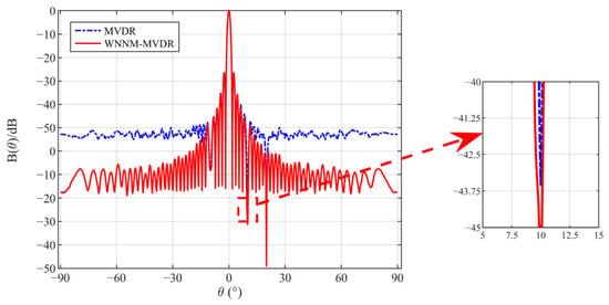
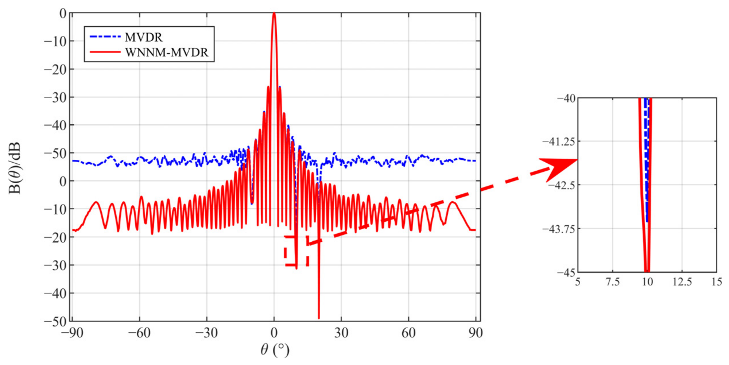
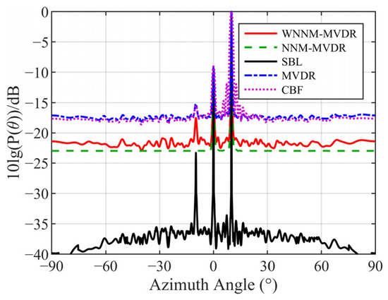
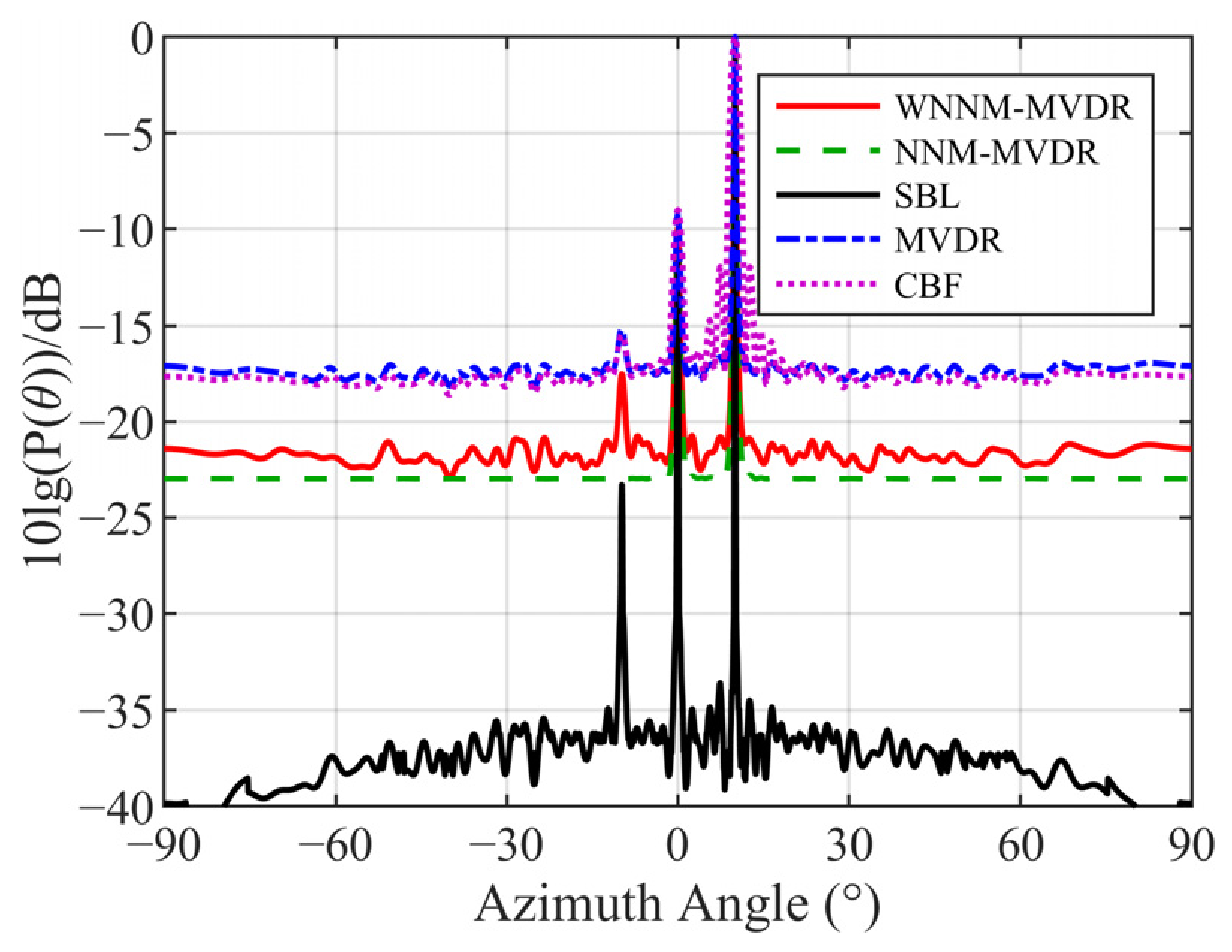
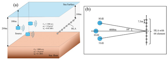
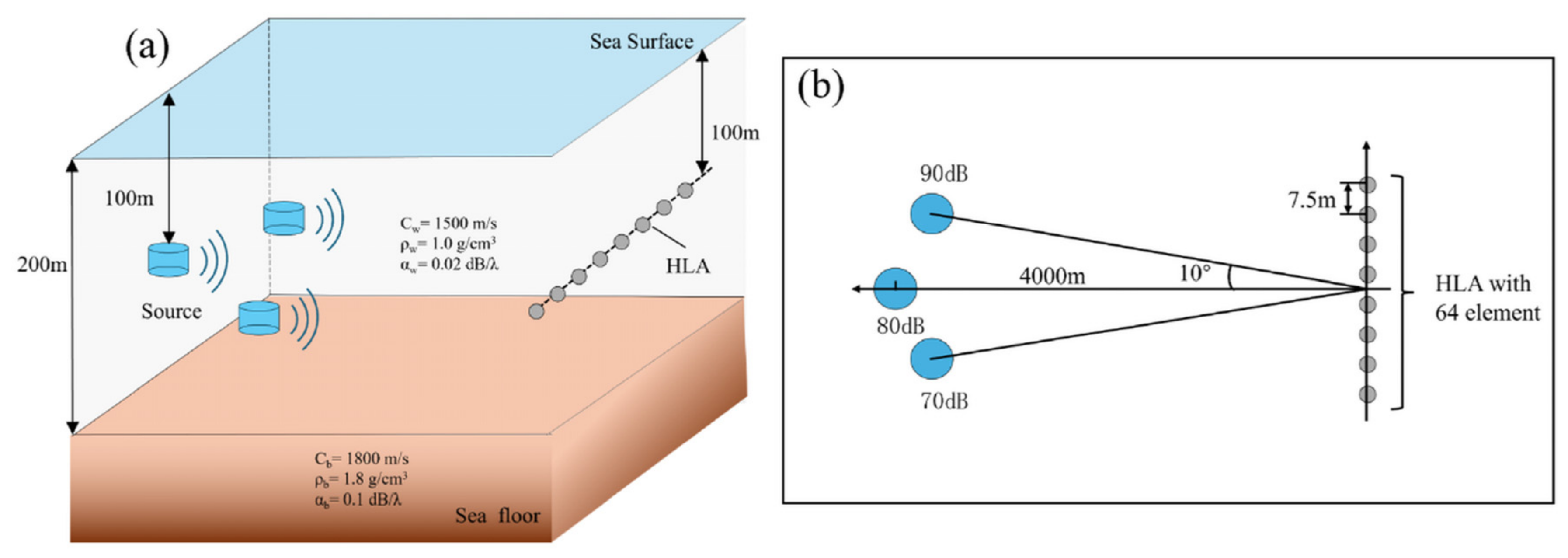
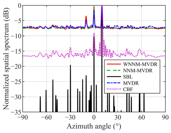
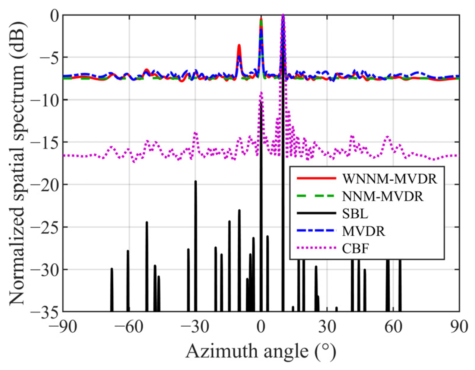
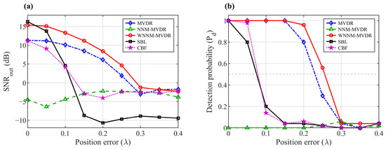
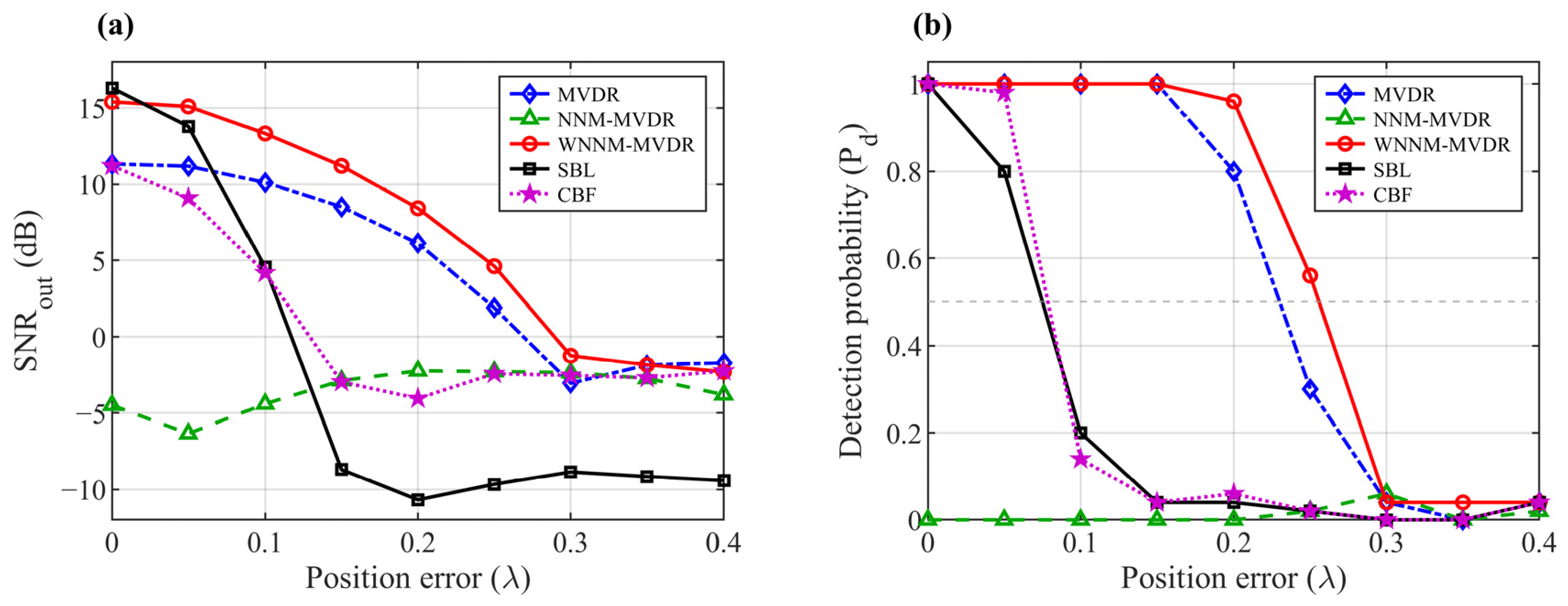
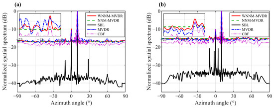
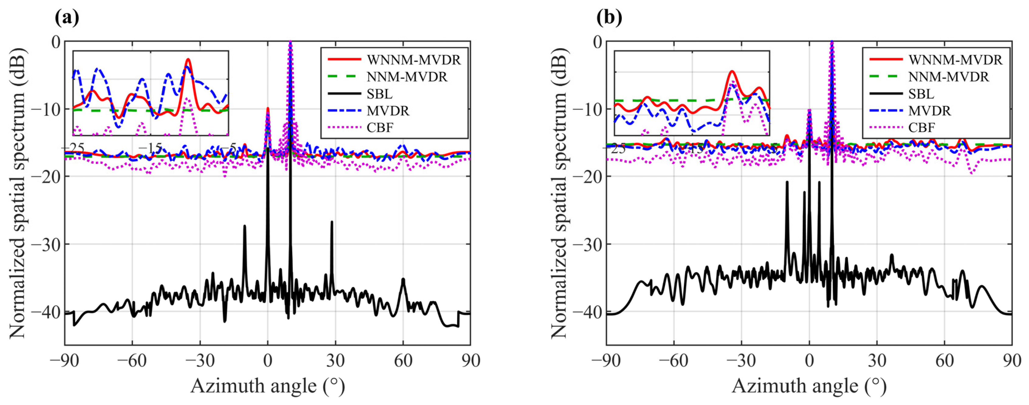
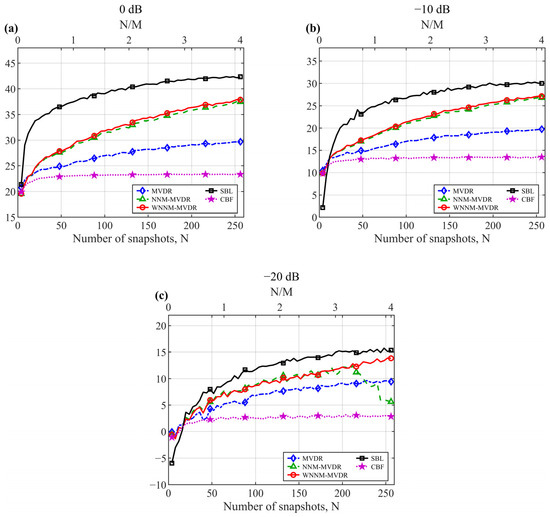
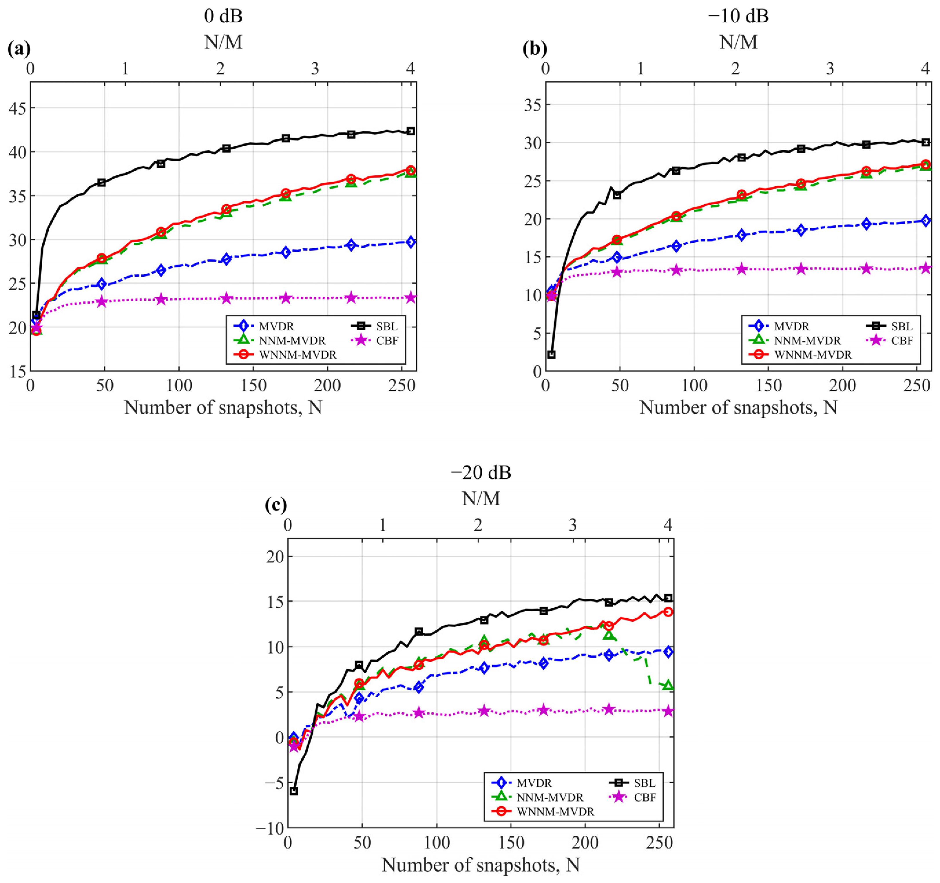
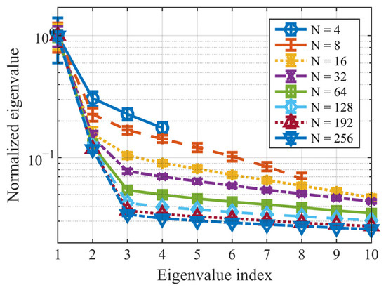
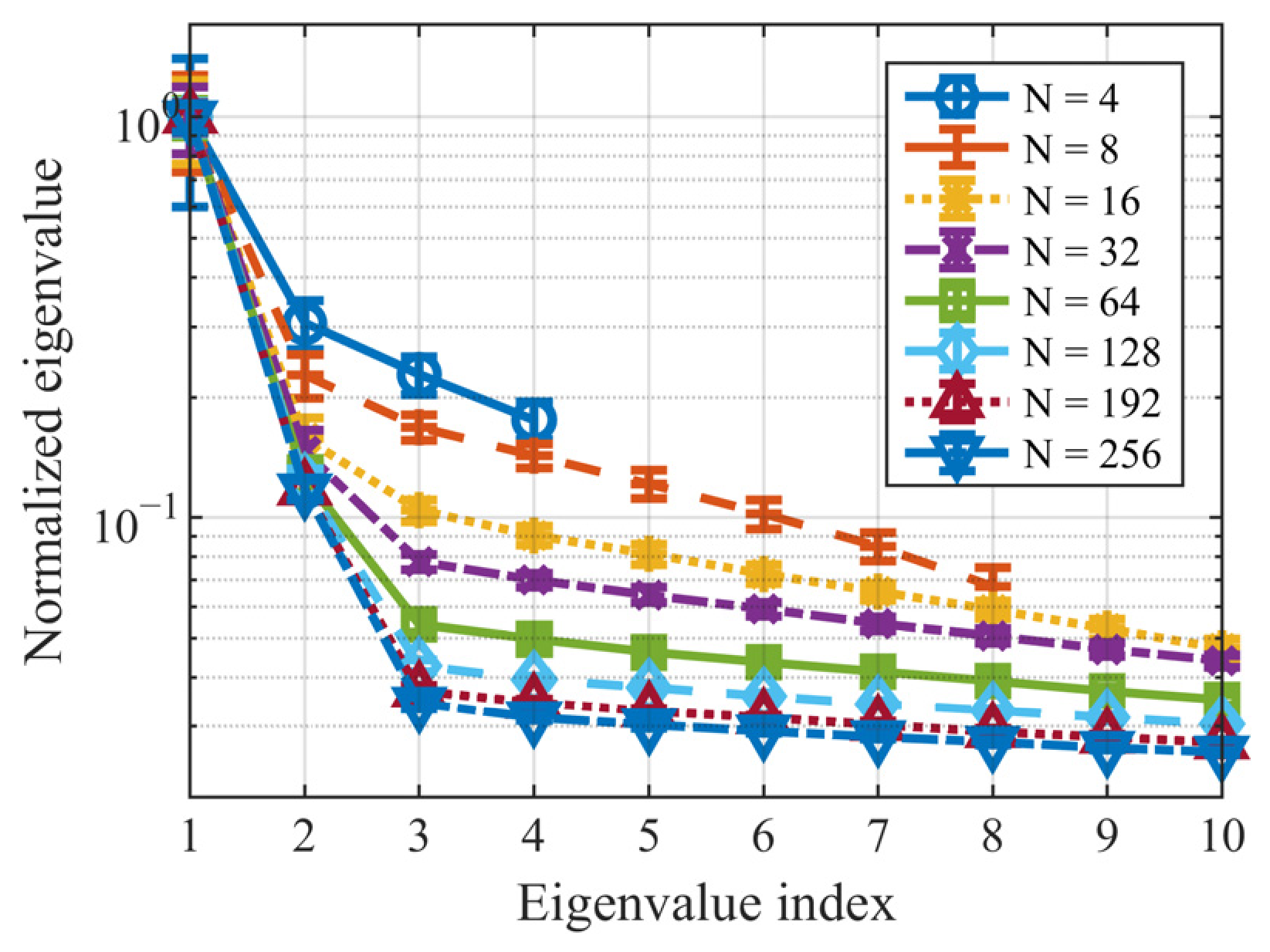
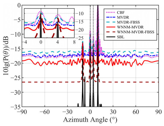
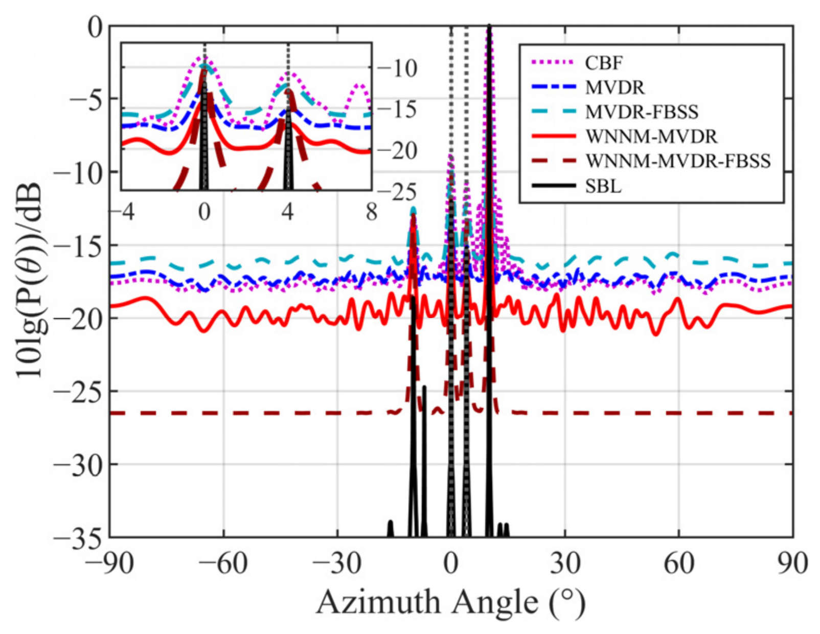
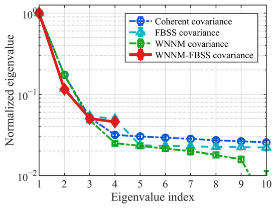
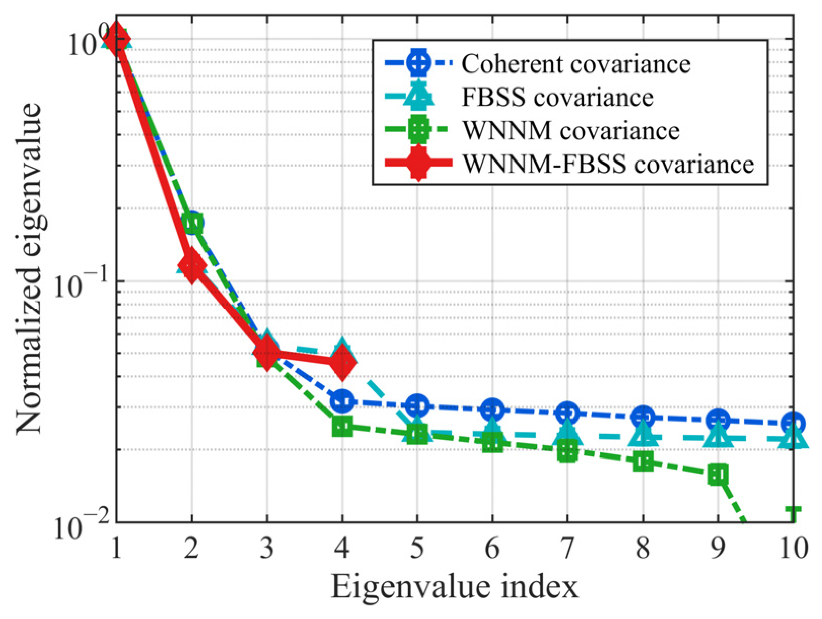
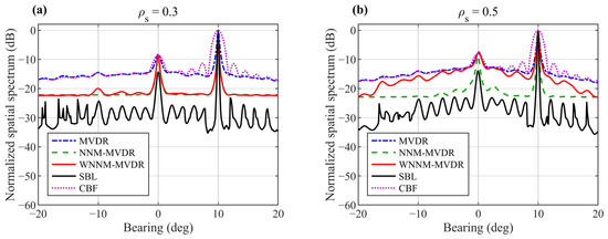
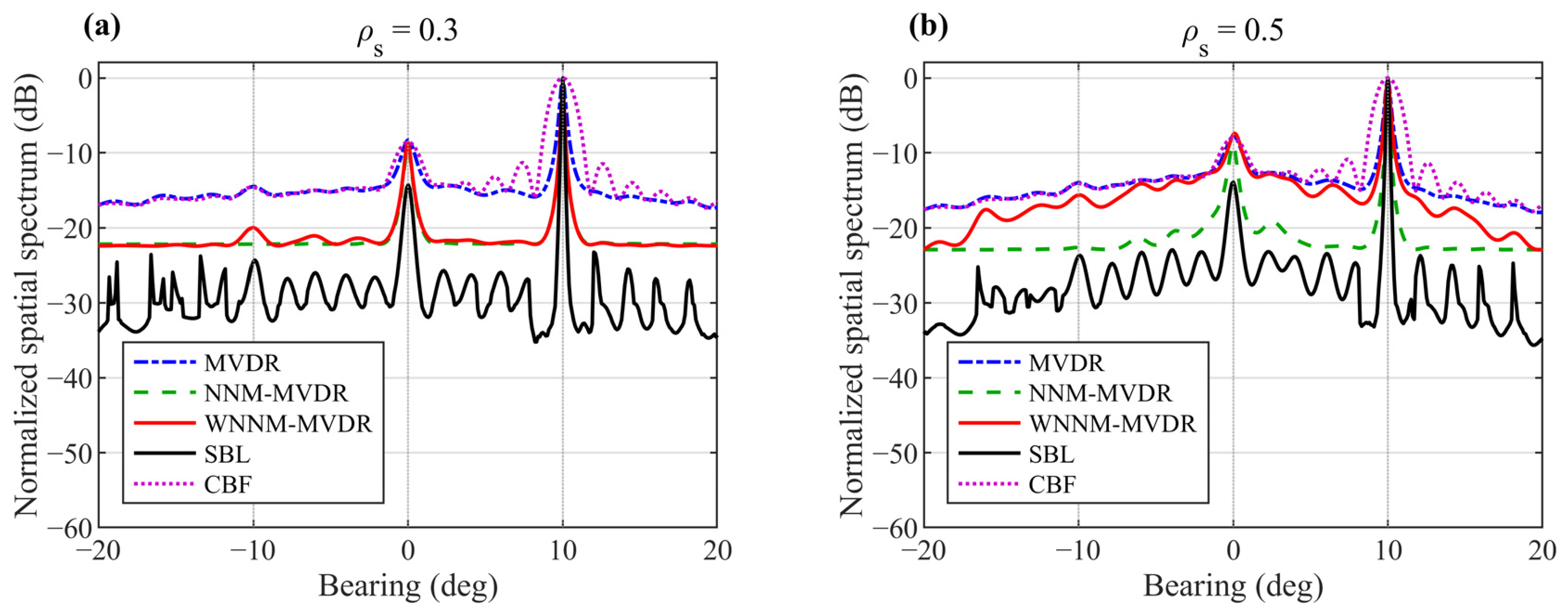
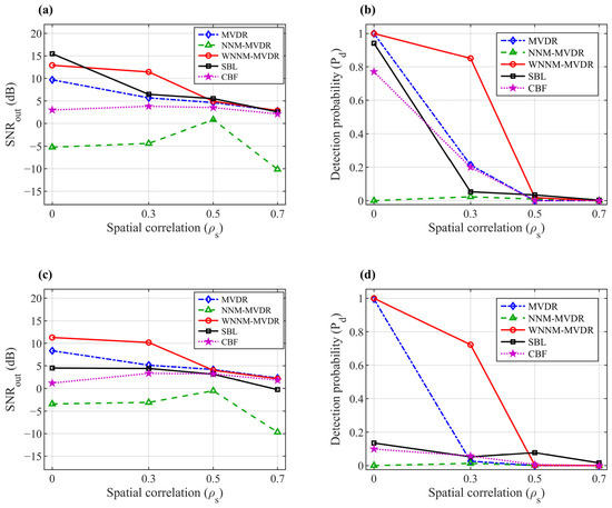
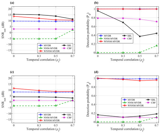
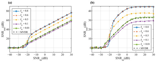
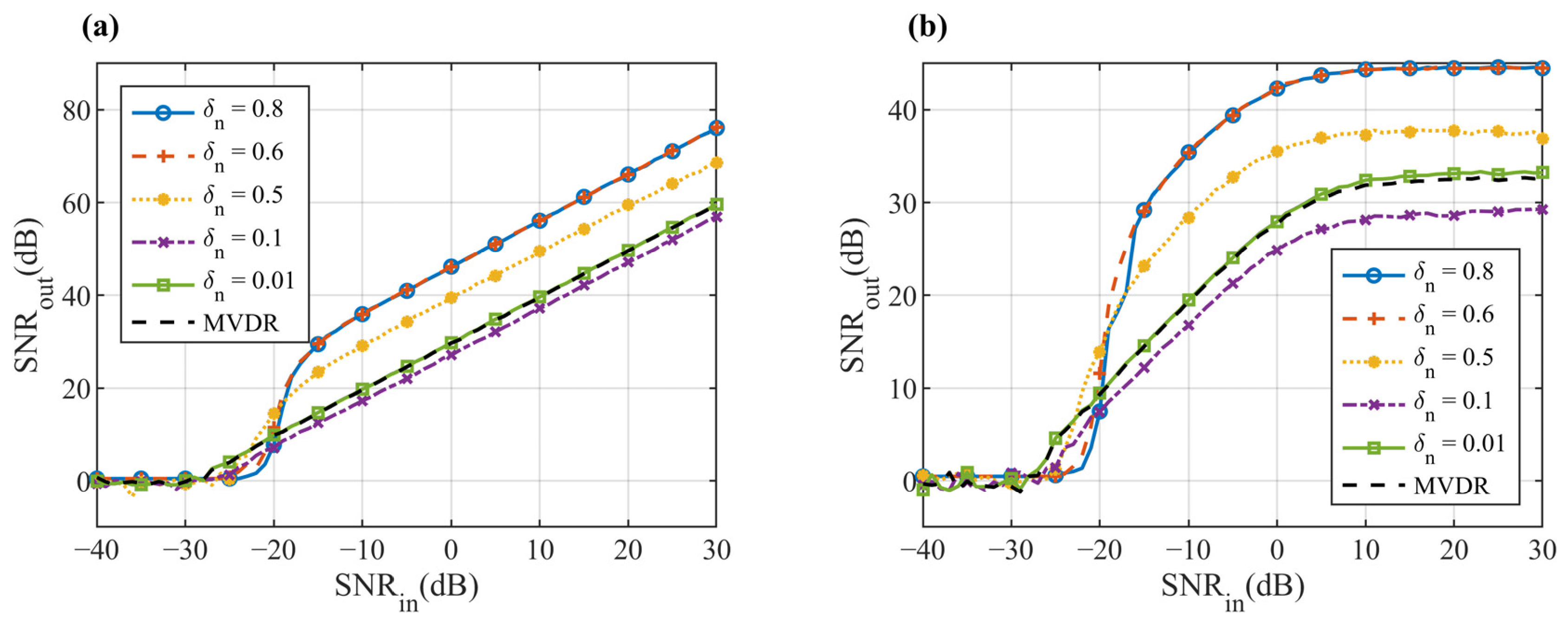
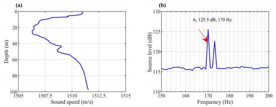
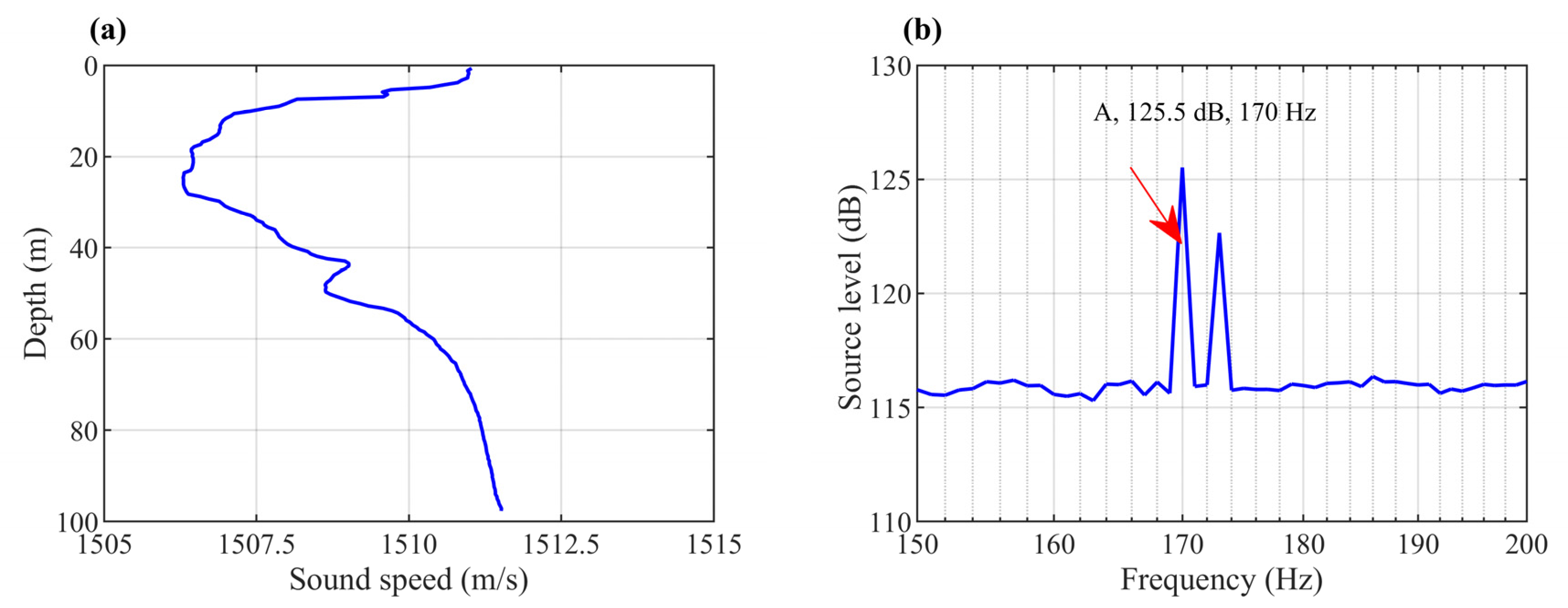
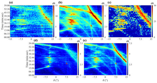
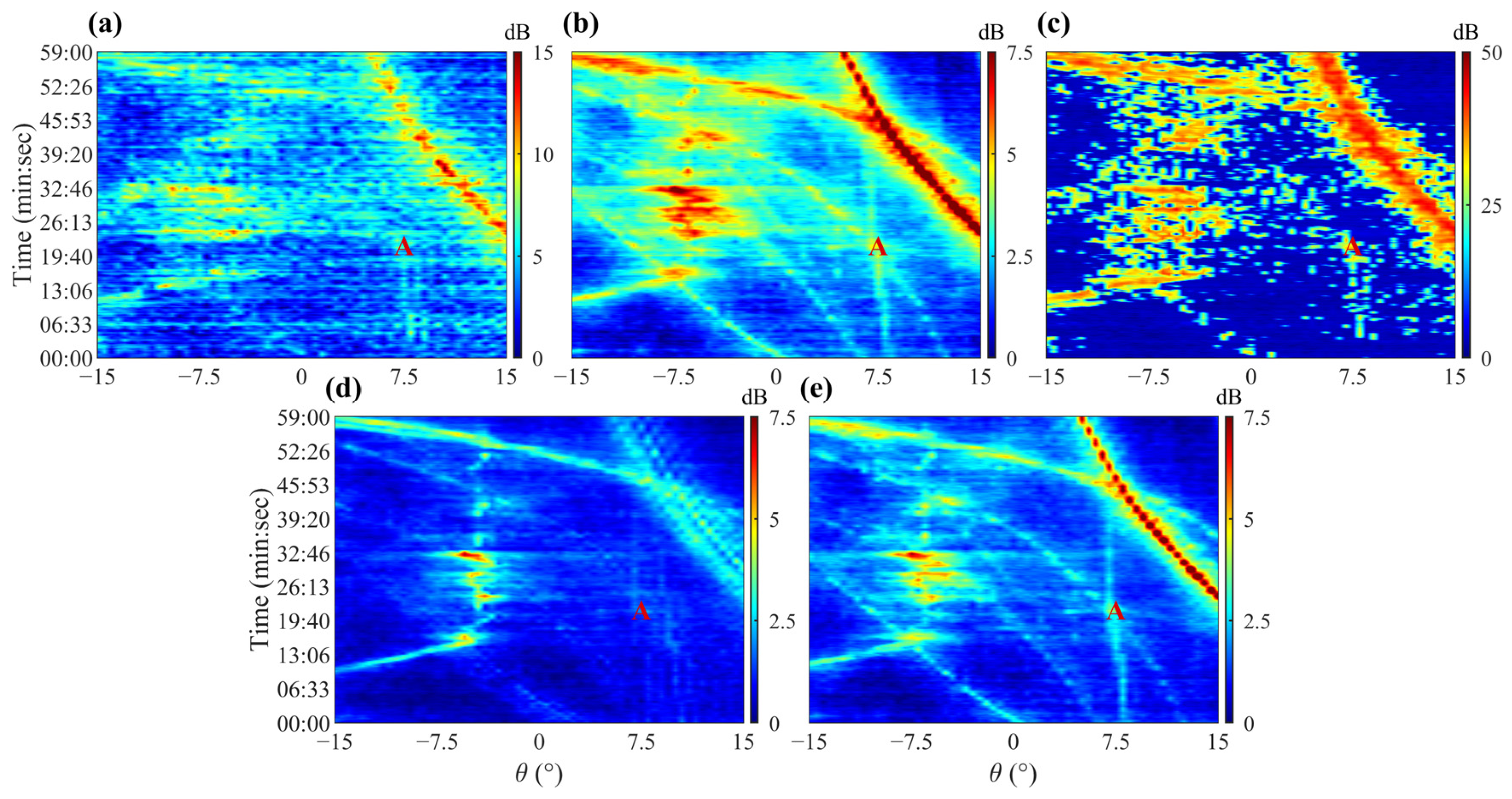
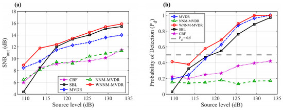
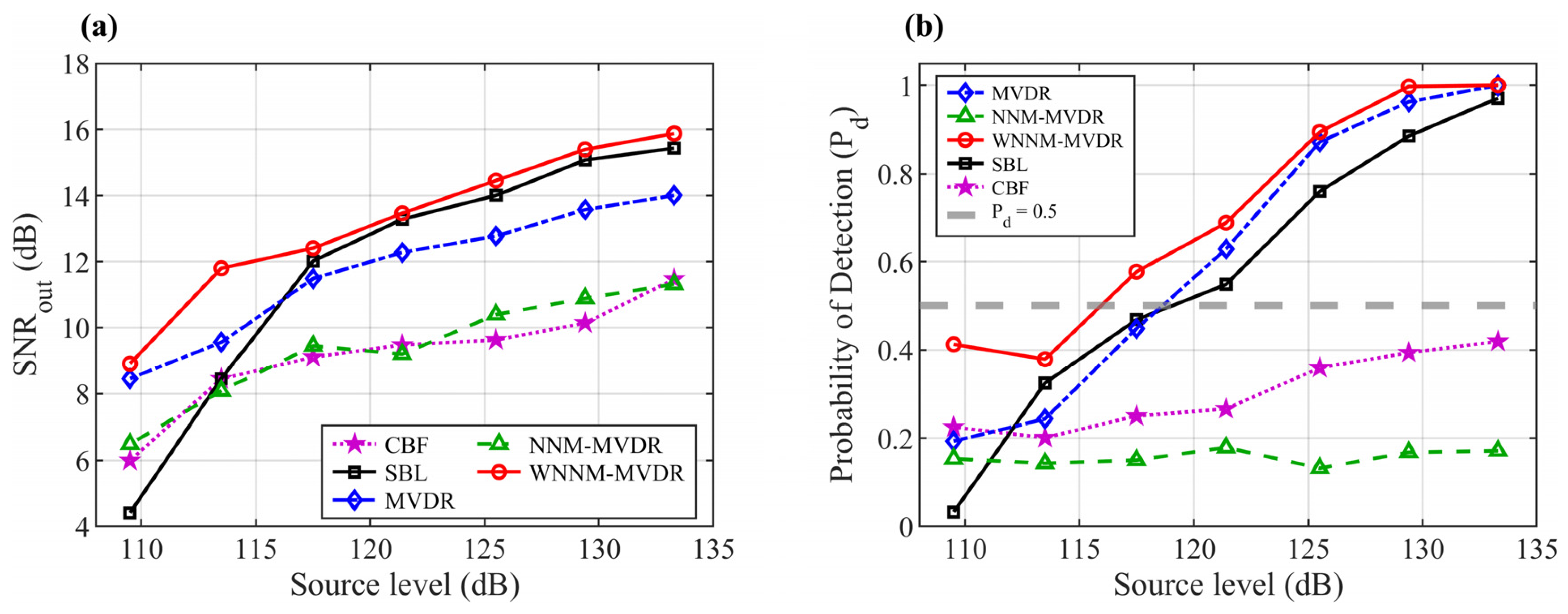
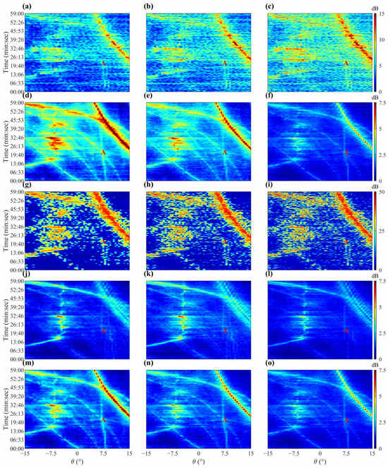
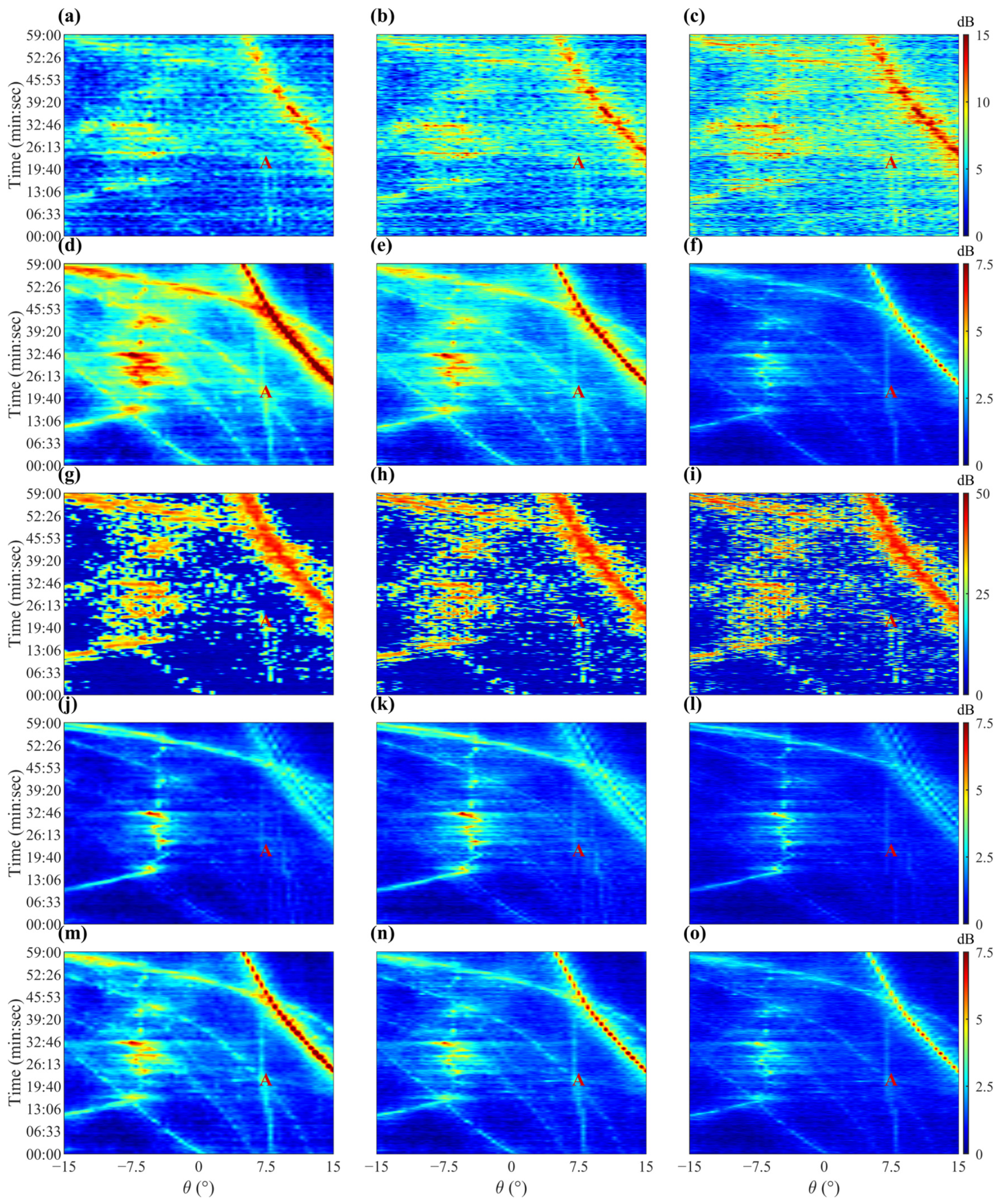
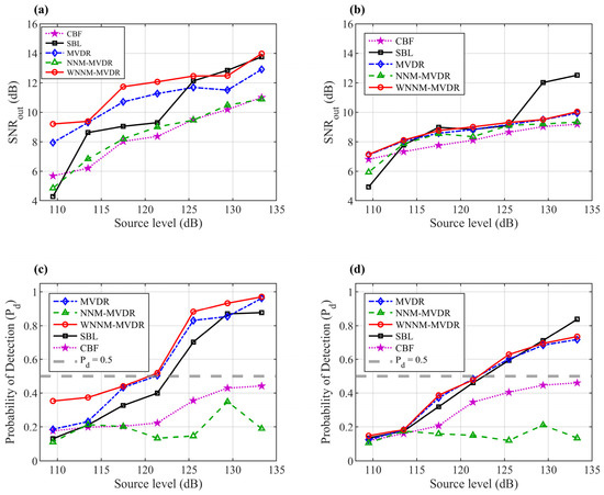
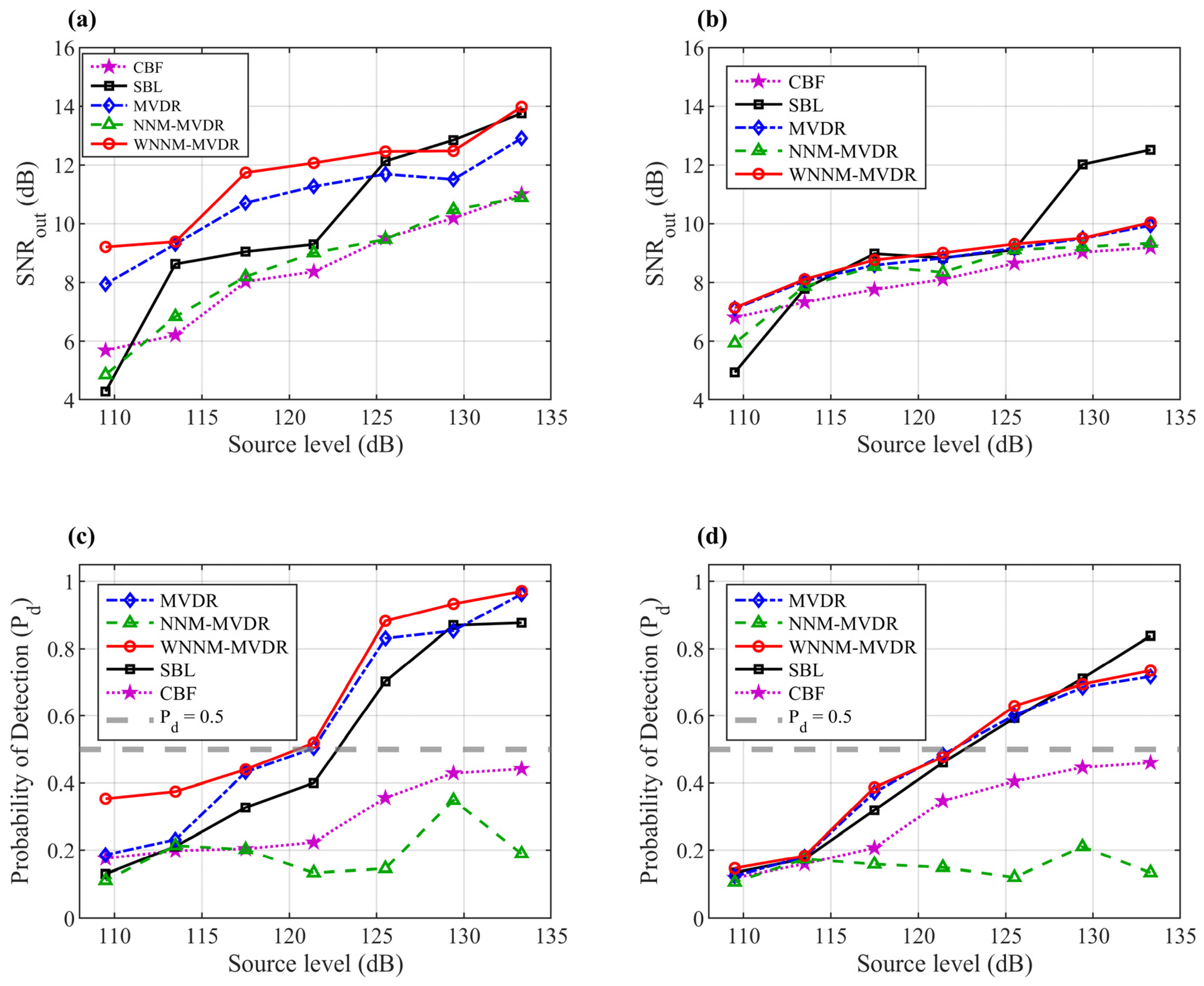
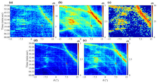
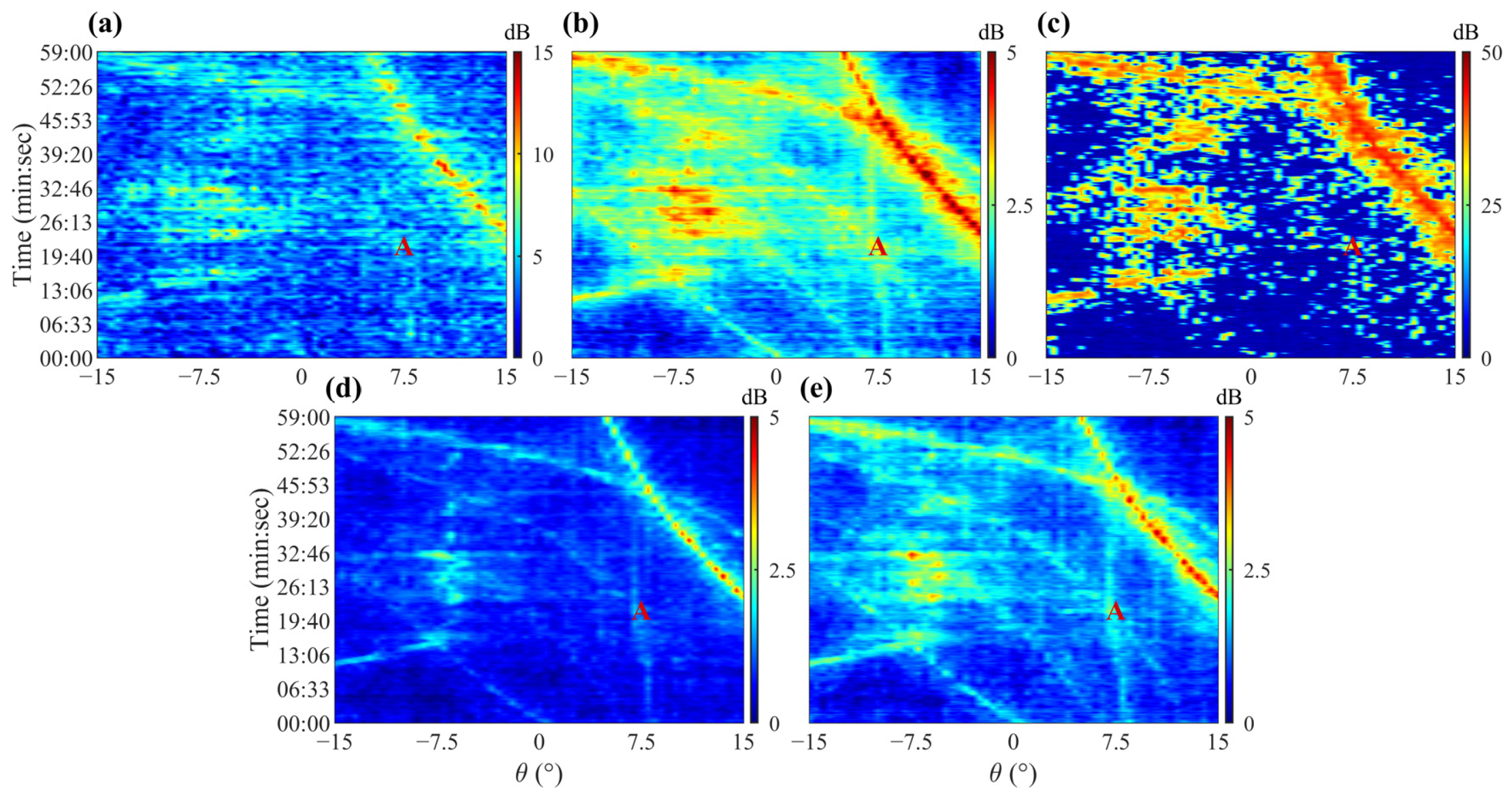
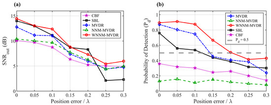
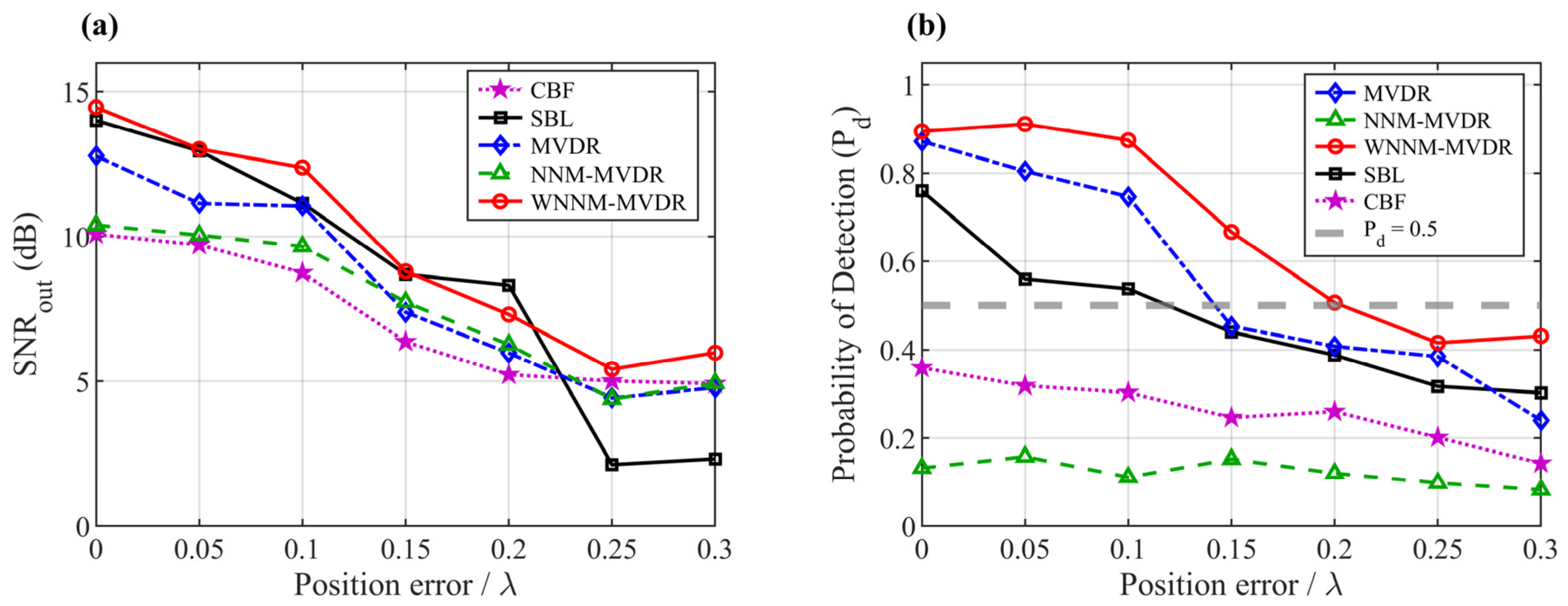

Disclaimer/Publisher’s Note: The statements, opinions and data contained in all publications are solely those of the individual author(s) and contributor(s) and not of MDPI and/or the editor(s). MDPI and/or the editor(s) disclaim responsibility for any injury to people or property resulting from any ideas, methods, instructions or products referred to in the content. |
© 2026 by the authors. Licensee MDPI, Basel, Switzerland. This article is an open access article distributed under the terms and conditions of the Creative Commons Attribution (CC BY) license.