


Abstract
Accurate maneuvering models are crucial for autonomous ships. Traditional methods such as model tests and CFD analysis require considerable time and cost to construct white-box models, while black-box models lack interpretability. Although system identification using operational data to identify white-box model parameters is efficient, standard maneuvers often lack sufficient excitation signals to yield generalizable models, and random maneuvers are impractical on full-scale ships. This study comparatively examines practical excitation signals that are easily implementable on full-scale ships to obtain informative data. Using pseudo-observation data of a KVLCC2 model ship, hydrodynamic coefficients of the MMG model are identified via a Markov Chain Monte Carlo (MCMC) method to quantify parameter uncertainty while explicitly accounting for observation noise. Among the tested cases, the linearly decreasing rudder-angle signal yielded the most balanced predictive performance for the turning and zig-zag maneuvers. In this numerical case study, the signal covered the full allowable rudder-angle range and generated motions ranging from turning to approximately straight-line behavior. The identified models also retained similar predictive accuracy under a specific synthetic perturbation introduced between the commanded and actual rudder angles. These results indicate that a linearly decreasing rudder-angle signal is a promising candidate for acquiring informative data for MMG model identification.
1. Introduction
In recent years, numerous studies have been conducted on the prediction of maneuvering motion with the objective of facilitating the practical implementation of autonomous ships [1,2,3,4]. Simulations based on maneuvering models that accurately represent the ship dynamics are effective in achieving advanced navigation tasks such as collision avoidance and berthing. White-box maneuvering models based on physical principles are the most conventional models. Representative white-box models are the Abkowitz model [5], the Fossen model [6], and the MMG model [7]. Conversely, many kinds of black-box models have been proposed, such as Neural Networks [8,9,10,11,12], Support Vector Machine [13,14], and the Gaussian Process [15,16]. However, these black-box models lack a physical foundation, which hinders their interpretability. Consequently, white-box models can be regarded as more appropriate than black-box models for incorporation into systems ensuring safe ship operations.
In order to fit a white-box model to the actual dynamics, it is necessary to properly identify the model parameters. Conventionally, parameter identification through tank tests, including captive model tests, has been a prevalent approach [7,17]. In addition, methodologies employing Computational Fluid Dynamics (CFD) analysis have been developed [18,19]. Although these methods can accurately identify model parameters for specific state of the ships, they require significant time and cost for experiments and analysis. Conversely, more efficient approaches have been proposed that utilize system identification methods to identify parameters from observation data of state variables. This approach enables the direct utilization of operational data from full-scale ships, eliminating scale effects that might arise from differences in Reynolds number between model and full scale. Åström and Källström determined the parameters of the Abkowitz model through the implementation of the Kalman filter [20]. Yoon and Rhee identified model parameters utilizing ridge regression in conjunction with estimation of the ship state using the Extended Kalman filter within the Estimation-Before-Modeling (EBM) framework [21]. Miyauchi et al. identified parameters of an MMG model, which is extended to be applicable in low-speed ranges such as during berthing and unberthing, using the Covariance Matrix Adaptation Evolution Strategy (CMA-ES) [22]. In contrast to these deterministic approaches, Xue et al. and Mitsuyuki et al. utilized Bayesian inference to estimate parameters as stochastic variables [23,24]. In these Bayesian inference-based methodologies, parameter identification is achieved through the utilization of prior knowledge concerning the potential range of parameters, under the assumption that observation data are affected by observation noise. In practical applications, this approach offers the advantage of quantifying parameter uncertainty based on the information of observation data and prior knowledge, while allowing observation noise to be represented explicitly in the probabilistic model.
Many studies on parameter identification for maneuvering models using system identification utilize observation data from the standard tests, such as the turning and zig-zag tests. However, while these standard tests have the advantage of being easy to conduct, the maneuvering motion patterns excited by these tests are limited. Therefore, from the perspective of system identification, these test data cannot be considered to contain sufficient excitation signals, and it is difficult for models identified from such data to predict maneuvers outside the identification dataset accurately. In order to address this issue, Nouri et al. and Wang et al. employed observation data from maneuvers based on Pseudo-Random Signals (PRSs) for parameter identification, instead of using standard test data [25,26]. The amplitude of the PRS and the holding time at a specific rudder angle were optimized. However, this optimization was predicated on the assumption that moderately accurate model parameters were known. This suggests that if the accuracy of the prior information is low, the optimized signals cannot be trusted. Miyauchi et al. employed observation data from maneuvers that were nearly random but required long-term data to obtain sufficient excitation signals [22]. Furthermore, from the perspective of ease of implementation on full-scale ships, random maneuvering methods are inferior to the standard tests.
As described above, it is critical for the identification of parameters in white-box models to employ observation data that are sufficiently enriched with excitation signals. However, there have been few investigations into excitation signals that can be easily implemented on full-scale ships, such as standard tests, while also yielding models with good predictive performance across the tested maneuvers. The present study examines practical rudder excitation signals suitable for accurate parameter identification of white-box maneuvering models. First, based on system identification, ship maneuverability, and practical feasibility, the candidate rudder excitation signals are presented. The candidate signals are comparatively evaluated in terms of posterior uncertainty and the predictive performance of the identified models for held-out standard-maneuver input histories. In the parameter identification stage, pseudo-observation data generated from those rudder excitation signals are used. Hydrodynamic coefficients of an MMG model are identified using a Bayesian inference framework utilizing the Markov Chain Monte Carlo (MCMC) method [24]. This method provides joint posterior samples and enables the quantification of parameter uncertainty. It should be noted that the present study assumes a normal operational condition with forward speed and focuses on maneuvering motion caused by the rudder.
2. Methodology
2.1. System Identification Framework
This study utilizes the MCMC-based method [24] to identify the hydrodynamic coefficients of the MMG model. This section briefly outlines the MMG formulation and the parameter identification method.
Yasukawa and Yoshimura constructed an MMG model [7]. The MMG model is expressed as in Equation (1). Definitions of coordinate systems are consistent with those provided in the original paper.
where and represent the ship mass, the added mass in the surge direction, and the added mass in the sway direction; and denote the moment of inertia and the added moment of inertia; and and r represent the surge velocity, sway velocity at the midship, and yaw rate. and N denote the surge force, the sway force, and the yaw moment. The subscripts and R represent the hull, propeller, and rudder. The hydrodynamic forces acting on the hull and are expressed as follows:
where and d denote the water density, the ship length between perpendiculars, and the draft; U is the resultant velocity defined as ; and and are the non-dimensionalized velocity components defined as and . and are the non-dimensionalized hydrodynamic coefficients on maneuvering. These parameters are simply referred to as hydrodynamic coefficients in this paper.
The hydrodynamic coefficients are identified using the MCMC method. Other parameters are assumed to be given. The distinct feature of this method is the acquisition of parameters not through a deterministic process, but rather through sampling from each posterior probability distribution. The following maneuvering model and observation model are employed in this method:
where denotes the true state variables at time t; represents the observed state variables at time t; denotes the control inputs consisting of the rudder angle and the propeller rotation speed; represents the model parameter vector; and denotes the observation noise following a zero-mean multivariate Gaussian distribution, with a covariance matrix . and are the standard deviations of the noise corresponding to each state variable. The MMG model is used as the function in the identification process.
The MCMC method [27] enables the acquisition of samples from multivariate posterior probability distributions. It is necessary to define the prior distribution for each parameter and how to calculate the likelihood of the observation data with a given parameter set. Given the observation dataset and assuming conditionally independent observation errors across observation times, the likelihood is defined as
where is obtained by integrating the MMG model for the parameter vector and the control-input history . The joint posterior distribution is then given by the following equation:
The No-U-Turn Sampler (NUTS) was used to draw samples from this joint posterior distribution. In the numerical implementation, the log likelihood was evaluated for numerical stability.
2.2. Criteria for Evaluating Rudder Excitation Signals
The accuracy of maneuvering models identified via the framework in Section 2.1 depends on the observation data used for the identification. From a system identification perspective, parameter identifiability degrades when input signals are limited to a narrow amplitude range or lack persistent excitation. Therefore, providing input signals that sufficiently excite the system is essential to isolate the distinct effects of each parameter. In addition, excitation inputs are subject to various constraints in practical ship operations. Unlike idealized settings in which arbitrary input signals can be prescribed, rudder inputs for full-scale ships are subject to operational, safety, and physical constraints. Therefore, the rudder excitation signal should be determined considering realistic operating conditions.
First, from the viewpoint of operational feasibility, excitation signals must be implementable by standard maneuvering procedures. Highly irregular or random inputs, such as pseudo-random binary signals, are generally difficult to execute in full-scale ship operations due to practical limitations in manual or automated control. This restricts the class of admissible input signals to relatively simple and structured time-series profiles.
Second, physical and safety constraints impose limits on the rudder actuation. The rudder angle is bounded within a finite range, and excessively rapid or discontinuous changes in the input may not be achievable due to actuator dynamics or may lead to unsafe ship motions. In addition, ship maneuvering dynamics inherently exhibit delayed responses to rudder inputs, which further constrains the effective excitation that can be introduced into the system.
Third, measurement and operational uncertainties must be considered. In real-world conditions, observation data are affected by noise, and the actual rudder motion may deviate from the commanded input due to disturbances and actuator imperfections. Therefore, candidate excitation signals should be evaluated in terms of whether they can provide informative data even when the executed rudder motion deviates from the commanded input.
Based on considerations of system identification and operational constraints, the following three criteria are used to compare the candidate excitation signals:
- Coverage of the full rudder angle range. The excitation signal should span a wide range of rudder angles in order to sufficiently excite different maneuvering regimes. Limiting the input to a narrow range results in insufficient variation in the observed states, which reduces the sensitivity of the data to certain parameters and degrades identifiability.
- Sustained excitation of nonlinear maneuvering dynamics. The input should continuously excite the system to induce diverse motion patterns rather than steady-state behavior. Maneuvers dominated by steady turning motion provide limited information for parameter identification, whereas inputs that induce transitions between different motion regimes increase the informativeness of the observed data.
- Consideration of response delay in ship dynamics. Since ship motion responds to rudder inputs with a certain delay, excitation signals must vary at a time scale that allows the system response to develop. Rapidly varying inputs may fail to effectively excite the dynamics, resulting in reduced information content in the data.
Guided by these criteria, representative candidate signals with different characteristics are introduced in the following section and subsequently compared through numerical experiments.
2.3. Candidate Rudder Excitation Signals
This section presents three specific candidate excitation signals. It should be noted that this study employs the commanded rudder angle as the excitation signal, assuming a constant propeller rotation speed. These signals are not obtained through an optimization procedure. Instead, they are selected as representative candidates to compare the effects of rudder-angle coverage and temporal variation on parameter identification.
Assuming a maximum rudder angle limit of 35 deg, the following three types of excitation signals are considered. The functions representing the commanded rudder angles for these signals are defined as follows:
where T denotes the period of the sine wave. The first method employs a constant maximum rudder angle. The commanded rudder angle remains at throughout the observation period and therefore has no temporal variation. The second method linearly decreases the rudder angle from the positive maximum to the negative maximum. This signal covers the full allowable rudder-angle range once while providing continuous temporal variation at a constant rate. The third method employs a sinusoidal variation with an amplitude equal to the maximum rudder angle. This signal periodically covers the full rudder-angle range, and its rate of variation depends on the period T. To examine the influence of the input time scale relative to the maneuvering response of the ship, periods of , 50, and are compared in the subsequent case study.
3. Case Study Setup
This numerical case study compares the candidate rudder excitation signals described in Section 2.3 in terms of their ability to produce models with accurate predictions for held-out maneuvering inputs. Pseudo-observation data generated from simulations by a known MMG model are utilized to identify the hydrodynamic coefficients. The predictive performance of the identified models is then evaluated using rudder-input histories obtained from turning and zig-zag simulations that were not used for parameter identification. This study adopts the root mean square error (RMSE) between the true and estimated trajectories at midship as a metric to evaluate the estimation results.
3.1. Target Ship
The target ship is the KRISO Very Large Crude Carrier 2 (KVLCC2) model ship, constructed at a scale of 1:45.7. Table 1 shows the principal particulars of the model ship. An MMG model of the model ship was identified by Yasukawa and Yoshimura [7]. In this case study, this MMG model is referred to as the “true model” and is employed to generate pseudo-observation data. Parameters other than the hydrodynamic coefficients are assumed to be the true values during identification.
Table 1.
Principal particulars of the KVLCC2 model ship.
3.2. Generation of Pseudo-Observation Data
Pseudo-observation data are generated by adding Gaussian noise to the time-series state variables obtained from simulations of the true model. The observed state variables are obtained using the observation model defined in Equation (3). In this case study, the standard deviations of the Gaussian noise are set to the following values:
The observation duration and sampling rate are set to 100 s and 1 Hz, respectively. The initial position and velocity components are set to zero except for the longitudinal velocity, which is 1.18 m/s. The propeller rotation speed is assumed to be constant at 17.95 rps. Regarding the initial rudder angle, the simulation is initialized at 0 degrees for the sinusoidal excitation, whereas it starts directly at the maximum angle of 35 degrees for the other candidate signals. It should be explicitly noted that initializing the simulation directly at the maximum rudder angle is a theoretical idealization. Numerical simulations for the pseudo-observation data generation are performed using OrdinaryDiffEq.jl version 7.8.1 with the Tsitouras 5/4 Runge–Kutta method, setting both the relative and absolute tolerances to . These numerical integration settings are identical to those used for the maneuvering motion predictions in Section 4.
In this case study, two distinct scenarios are considered. The first scenario involves an ideal condition in which the rudder moves exactly as commanded according to Equation (6). The actual rudder angle variation is identical to the commanded rudder angle in this scenario. The second scenario introduces a synthetic discrepancy between the commanded and actual rudder angles to examine the sensitivity of the identification results to imperfect input execution. Specifically, noise is added to the commanded rudder angle values at 0.1-s intervals. The actual rudder angle variation is generated by interpolating these points using cubic spline interpolation, which is utilized to generate the pseudo-observation data. The noise applied to the rudder angle is modeled as Gaussian noise with a mean of 0.0 deg and a standard deviation of 5.0 deg. This scenario does not employ a physical actuator model incorporating realistic response lags and rate limits; rather, it is intended strictly to evaluate the sensitivity of the identification results to the specific synthetic perturbation. During the identification of the hydrodynamic coefficients, only the commanded rudder angle is assumed to be known, whereas the actual noisy rudder angle is regarded as unknown.
3.3. MCMC Settings
Uniform distributions are adopted as the prior distributions for the hydrodynamic coefficients, and . The prior distributions for the hydrodynamic coefficients are set according to Equation (8), following the database of hydrodynamic coefficients summarized by Yoshimura et al. [28]. They are specifically configured to cover the range of hydrodynamic coefficients for tankers, bulk carriers, and container ships in the database. The range of the uniform distribution for the standard deviations and is set from 0.0 to 1.0. The No-U-Turn Sampler (NUTS) [29] was used to sample from the joint posterior distribution. The sampler was implemented using Turing.jl [30] version 0.46.0 with Julia version 1.12.6. For each identification case, four independent chains were run using independent random seeds. Each chain consisted of 1000 warmup iterations followed by 1000 retained draws, yielding a total of 4000 post-warmup draws. The initial samples were randomly generated from each prior distribution. The target acceptance probability was set to 0.9, and the maximum tree depth was set to 10. The sampled parameters consisted of the 17 hydrodynamic coefficients and the three observation-noise standard deviations, , , and .
Sampling convergence was assessed using the rank-normalized split statistic, the bulk and tail effective sample sizes (ESSs), and the numbers of divergent transitions and transitions that reached the maximum tree depth.
4. Results
4.1. Hydrodynamic Coefficient Identification Using Pseudo-Observation Data Generated from Ideal Rudder Profile
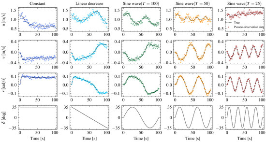
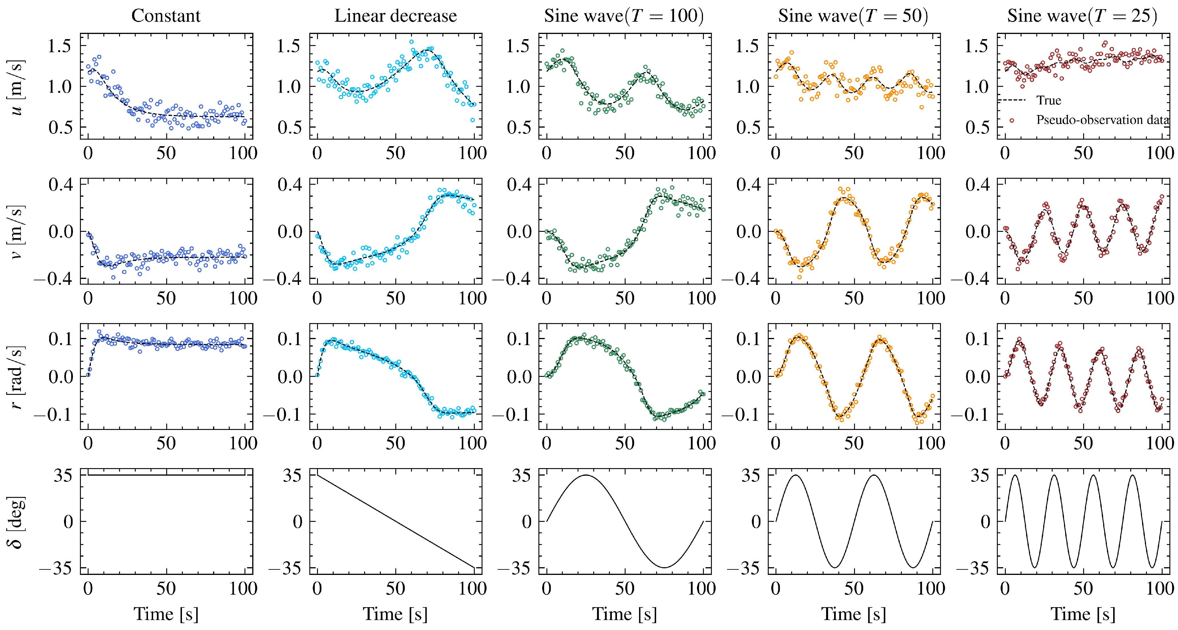
In this section, an ideal case scenario is examined wherein the actual rudder angle exactly moves as commanded according to Equation (6). The objective is to compare the candidate excitation signals in terms of the predictive performance of the resulting models for held-out maneuvering inputs. Figure 1 shows the pseudo-observation data and the actual rudder angle variation. The black dashed lines represent the true values of velocity components. There are five sets of maneuvering data corresponding to five different excitation inputs. It should be noted that each of these data is utilized independently for the identification of the hydrodynamic coefficients.
Figure 1.
Pseudo-observation data and time series of rudder angle.
Table 2 summarizes the sampling diagnostics for the five ideal-input cases. For each case, the maximum and the minimum bulk and tail effective sample sizes (ESS) were calculated over all 20 inferred parameters. Across the five ideal-input cases, the largest value was 1.004, while the minimum bulk and tail ESS values were 1221 and 1305, respectively. No divergent transitions or transitions reaching the maximum tree depth were observed. These diagnostics indicate satisfactory mixing and numerical convergence of the four chains. In addition, no significant dependence on the initial sample values was observed under the initialization conditions investigated in this case study. The corresponding trace plots are presented in Appendix A.
Table 2.
MCMC sampling diagnostics for the ideal-input cases. The maximum and the minimum bulk and tail ESSs were calculated over all 20 inferred parameters.
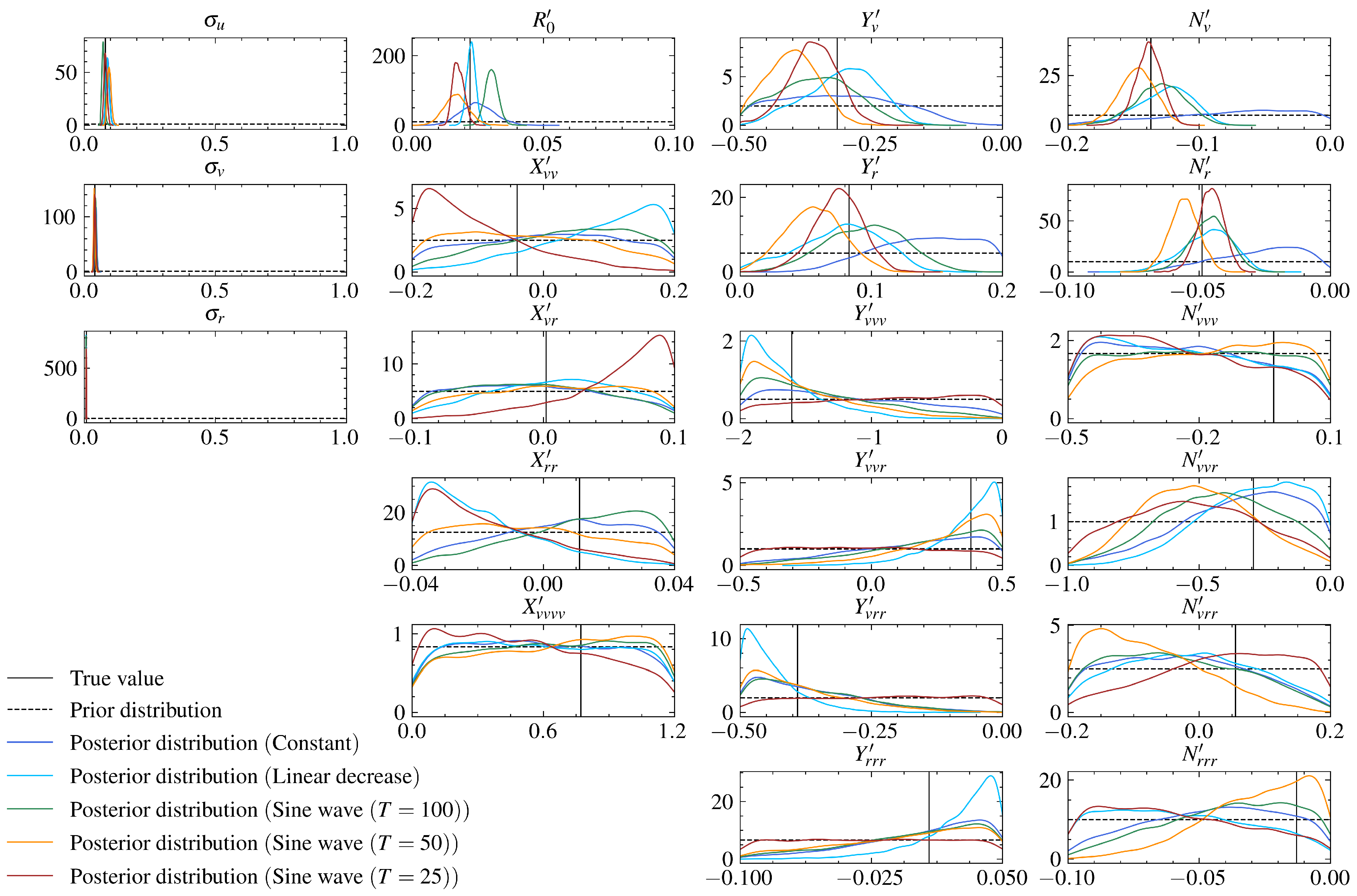
Figure 2 illustrates the prior and posterior probability distributions of hydrodynamic coefficients and observation-noise standard deviations identified from these pseudo-observation data. Since the MCMC method provides only discrete samples of parameters, the posterior probability distributions are approximated using Kernel Density Estimation (KDE). The vertical black line, the black dashed line, and the colored lines represent the true value, the prior distribution, and the posterior distribution of each parameter, respectively. Distinct peaks are observed in the posterior distributions of and the first-order hydrodynamic coefficients and with their locations close to the true values for almost all maneuvering data. However, no distinct peaks are observed in the posterior distributions of the first-order hydrodynamic coefficients identified from the maneuvering data obtained with a constant rudder angle. This is because the maneuvering motion under a constant rudder angle rapidly reaches a steady state, severely diminishing the parameter identifiability and resulting in limited updates from the prior distribution. Furthermore, for several higher-order hydrodynamic coefficients, either no clear peak is observed or the peak deviates from the true value. This phenomenon is likely influenced by the correlations between terms of second order or higher in the polynomial representing the forces acting on the hull, as shown in Equation (2). Such potential correlations can make it difficult to distinguish the contributions of each term and identify the hydrodynamic coefficients.
Figure 2.
Prior and posterior distributions of hydrodynamic coefficients and observation-noise standard deviations.
In addition to the presence or absence of distinct peaks, the spread of the posterior distributions provides further insight into parameter identifiability. For the lower-order hydrodynamic coefficients, the posterior distributions obtained from sinusoidal excitation tend to exhibit narrower spreads compared to those from constant and linearly decreasing inputs. This suggests that the periodic nature of the sinusoidal input enhances sensitivity to these parameters, allowing them to be more tightly constrained by the observed data. In contrast, for higher-order hydrodynamic coefficients, the linearly decreasing input occasionally results in relatively narrower posterior distributions compared to other excitation signals. However, the reduction in uncertainty is less pronounced than that observed for lower-order coefficients, and the observed differences among the excitation signals appear limited. This suggests that the identification of higher-order coefficients may be affected by correlations among the polynomial terms in the model structure. This highlights that the effectiveness of excitation signals should be evaluated not only by the location of posterior peaks but also by the degree of uncertainty reduction.
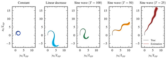
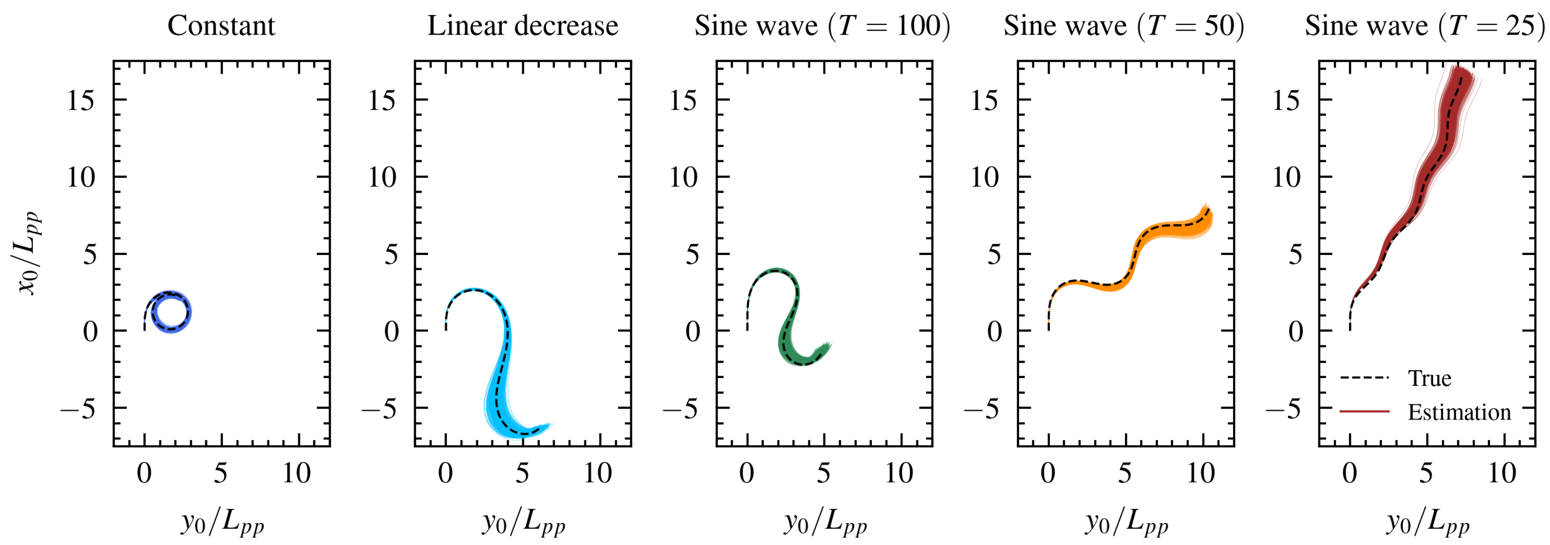
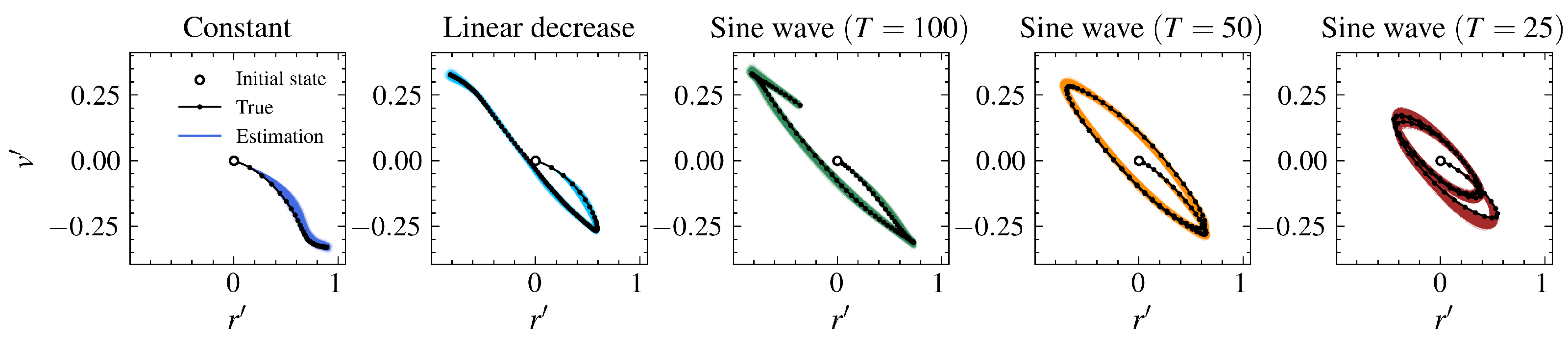
Here, it is verified that MMG models containing these samples of hydrodynamic coefficients can reproduce the maneuvering motions used for identification when the excitation signals shown in Equation (6) are given. Figure 3 shows the true and estimated trajectories. In all cases, the estimated trajectories are distributed close to the true trajectories, indicating that the identified MMG models accurately fit each maneuvering motion. Figure 4 shows the phase portraits for each candidate excitation signal. The white points edged in black indicate the initial states, the black points are plotted at 1-s intervals, and the black lines represent the true paths of the velocity components. This figure focuses on lateral motion, and both axes are non-dimensionalized. Based on these results and Figure 2, it is confirmed that although the true values of the hydrodynamic coefficients have not been captured, hydrodynamic coefficients capable of reproducing the maneuvers used for identification have been obtained.
Figure 3.
Estimated trajectories under each candidate rudder input using the identified models.
Figure 4.
Estimated phase portraits under each candidate rudder input.
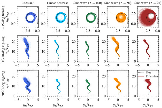
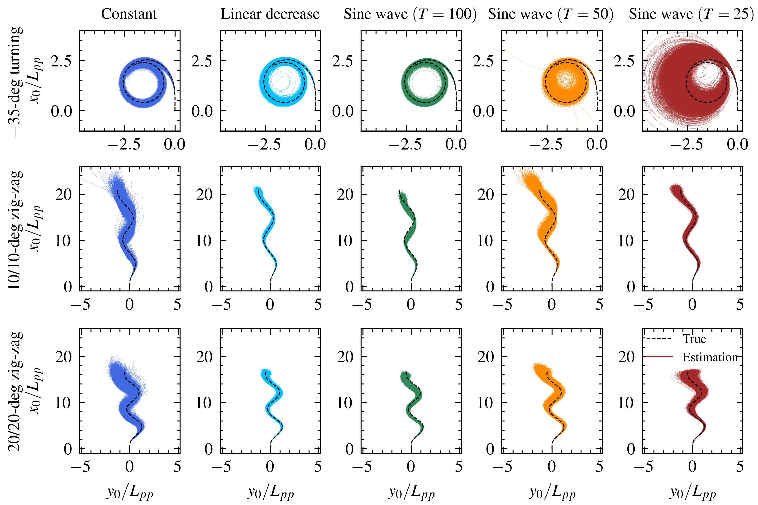
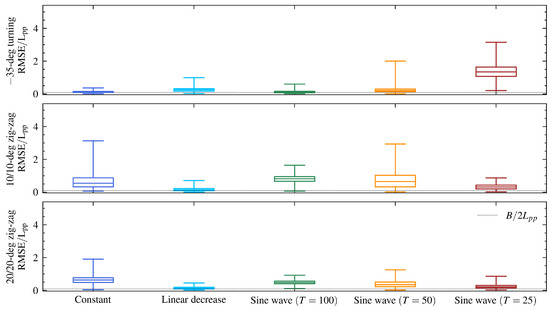
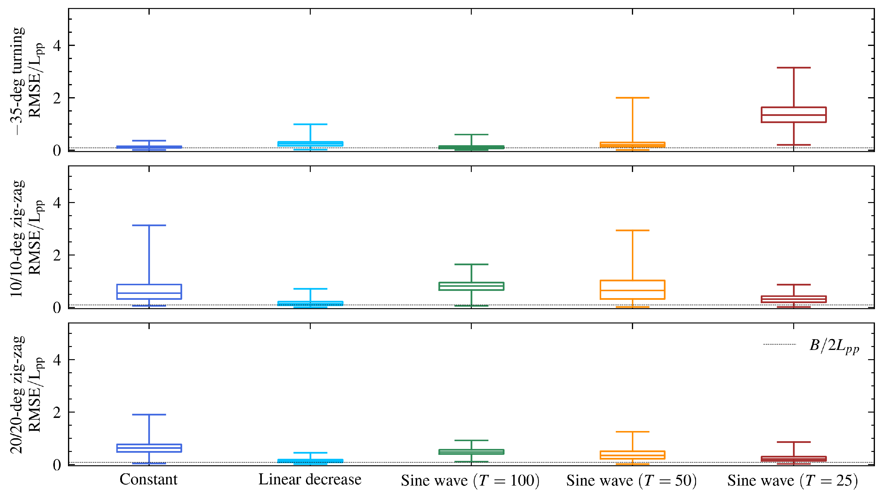
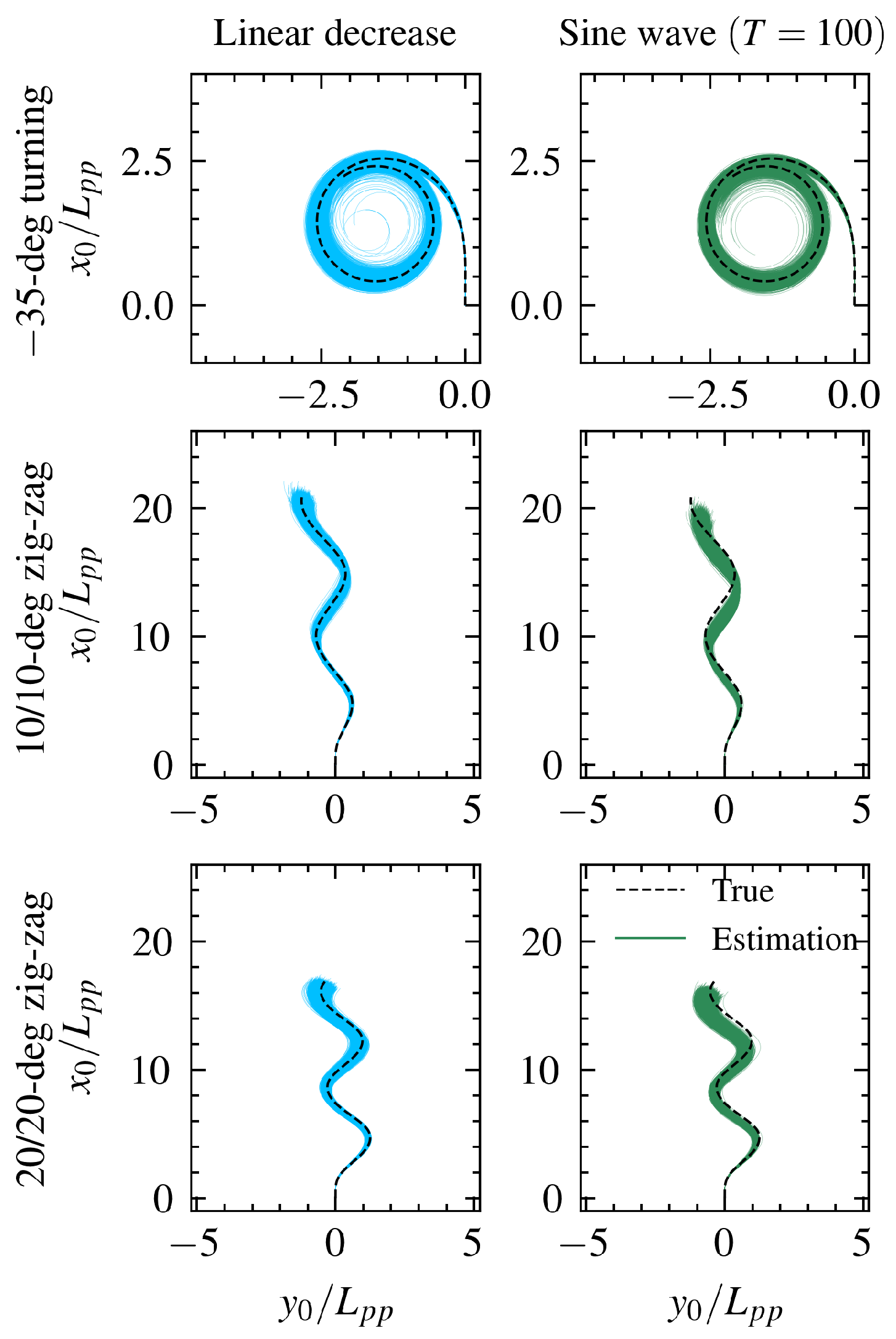
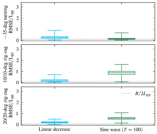
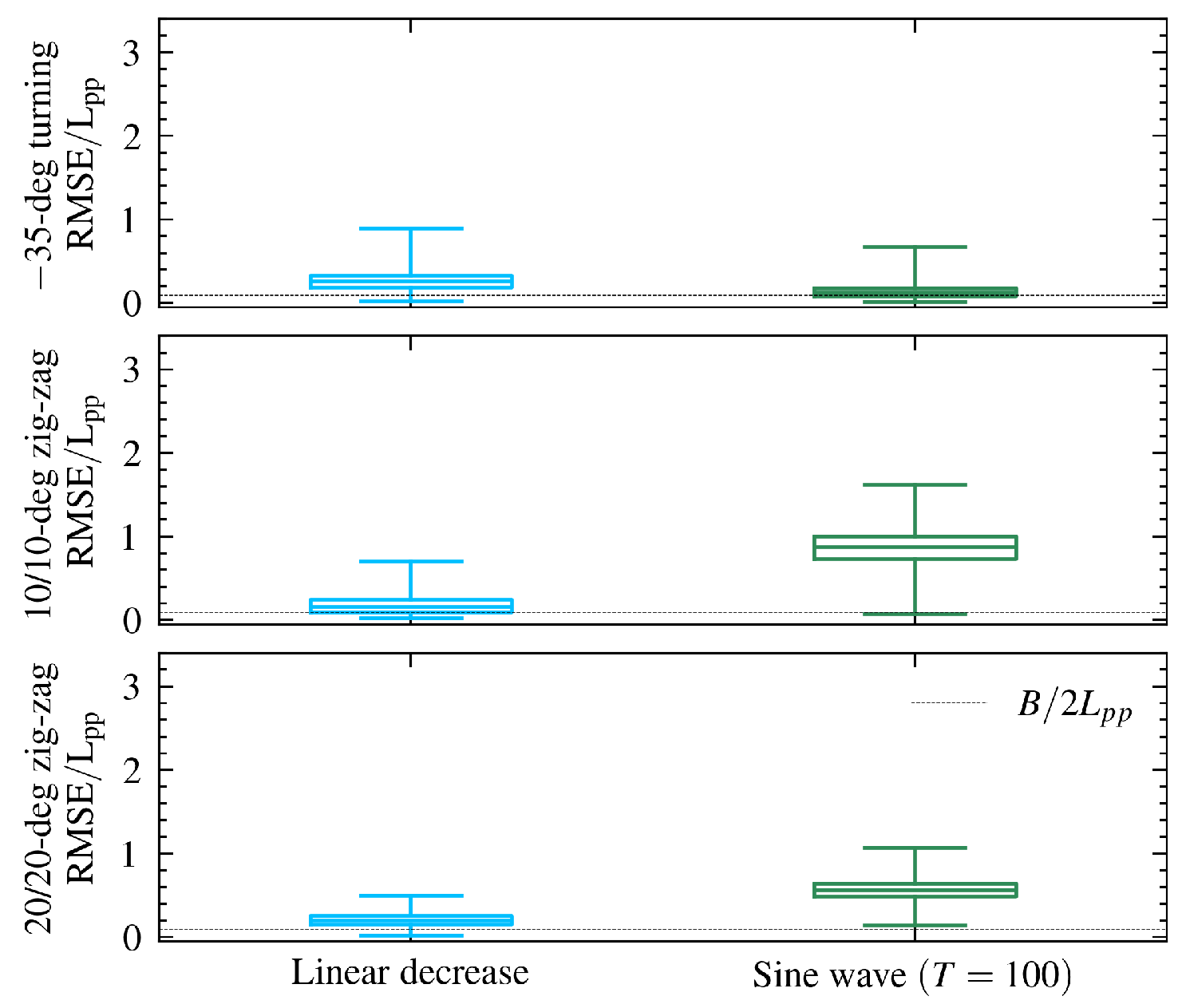
Next, the cross-maneuver predictive performance of the identified MMG models is evaluated using held-out rudder-input histories obtained from a −35-deg turning simulation, a 10/10-deg zig-zag simulation, and a 20/20-deg zig-zag simulation. The rudder angle variations used for these predictions are identical to those obtained from simulations of each test using the true model. Figure 5 shows the predicted trajectories of the three standard tests using 4000 MMG models obtained from each maneuvering dataset. Both axes are non-dimensionalized by the ship length between perpendiculars, . Figure 6 illustrates boxplots of RMSEs between the true and estimated trajectories, both of which are non-dimensionalized by . To preserve visual clarity, predictions that resulted in numerical divergence are excluded from the visualizations in Figure 5 and Figure 6. For all successfully completed simulations, however, the boxplots include every prediction result without any outlier exclusion or data truncation; the whiskers represent the exact minimum and maximum calculated RMSEs. The horizontal dotted line represents , where is the half-breadth of the target ship, non-dimensionalized by . Table 3 provides the numerical summaries of the prediction errors, consisting of the median and 95th percentile RMSE values alongside the number of divergent cases. A small RMSE value indicates that the model’s dynamics are close to those of the target ship. Within the present case study, consistently small RMSE values across the three held-out maneuvers are interpreted as indicating better cross-maneuver predictive performance.
Figure 5.
Predicted trajectories of −35-deg turning, 10/10-deg zig-zag, and 20/20-deg zig-zag.
Figure 6.
Boxplots of non-dimensionalized RMSEs between the true and predicted trajectories.
Table 3.
Median and 95th percentiles (P95) of the non-dimensionalized RMSEs and the number of numerical divergences.
MMG models identified from maneuvering data with the constant signal demonstrated the smallest median RMSE value and variance during the −35-deg turning test, indicating high prediction accuracy. However, these MMG models exhibited poor prediction accuracy in the zig-zag tests, indicating poor predictive performance for the held-out zig-zag maneuvers. This is because the first-order maneuvering hydrodynamic coefficients that dominate motion prediction in the zig-zag tests [31] were not captured accurately since the constant rudder angle did not provide sufficient excitation signals. In contrast, the MMG models identified from the maneuvering data with the linearly decreasing signal produced relatively small RMSEs for both the turning and zig-zag maneuvers, resulting in the most balanced predictive performance among the tested cases. As can be seen from the trajectories in Figure 3, when the rudder angle decreases linearly, both turning and straight-line motions are excited. This broader variation in the motion history is consistent with the relatively balanced predictive performance observed for the linearly decreasing input. The MMG models identified from maneuvering data with the 100-s-period sinusoidal signal also exhibited relatively balanced performance. However, the prediction accuracy for the zig-zag tests is lower than that of the models identified from maneuvering data with the linearly decreasing rudder angle because the excitation related to straight-line motion is insufficient. Furthermore, when the sinusoidal period is 50 or 25 s, the predictions by some of the identified models show significant deviation in the turning test. Since ships respond slowly to rudder angle input, changes in the rudder angle do not quickly affect the ship motion. Therefore, even when the full range of maximum rudder angles is covered, short-period rudder angle variations cannot sufficiently excite the corresponding response, degrading parameter identifiability and preventing the acquisition of appropriate parameters. These results suggest that the three criteria should be considered jointly when comparing the tested signals.
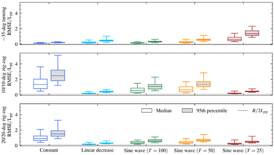
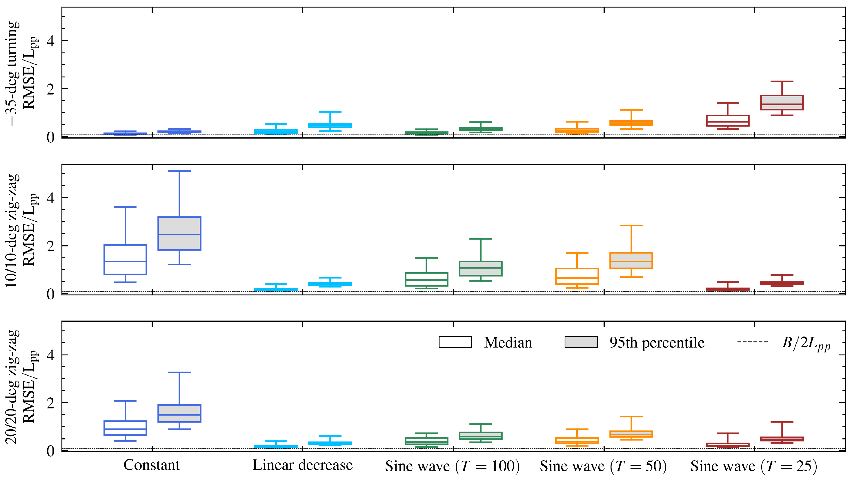
The preceding analysis evaluated the predictive performance based on a single realization of the pseudo-observation noise. To ensure that the presented performance is not an artifact of a specific noise pattern, the identification process was repeated across 100 independent observation-noise realizations for each candidate signal. For each noise realization and excitation signal, the held-out turning and zig-zag maneuvers were predicted using the 1000 parameter samples from a single MCMC chain. The prediction errors were then summarized by computing the median and 95th percentiles of the RMSEs between the true and predicted trajectories, excluding any samples that resulted in numerical divergence.
Figure 7 displays boxplots of the median and 95th percentile RMSEs across the 100 noise realizations for each excitation signal. The MMG models identified from maneuvering data with the linearly decreasing signal consistently produce low median RMSEs for both turning and zig-zag maneuvers. Furthermore, the 95th percentile RMSEs for this signal remain relatively low and stable across the different noise patterns. In contrast, the MMG models identified from observation data with the other excitation signals demonstrate larger median and 95th percentile RMSEs for the zig-zag maneuver. In contrast, the models identified using the other excitation signals exhibit limitations: the 25-s-period sinusoidal signal yields larger RMSEs for the turning maneuver, whereas the constant and longer-period sinusoidal signals produce larger errors for the zig-zag maneuvers.
Figure 7.
Boxplots of the median and 95th percentiles of the non-dimensionalized RMSEs across the 100 noise realizations for each excitation signal.
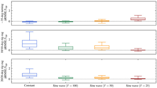
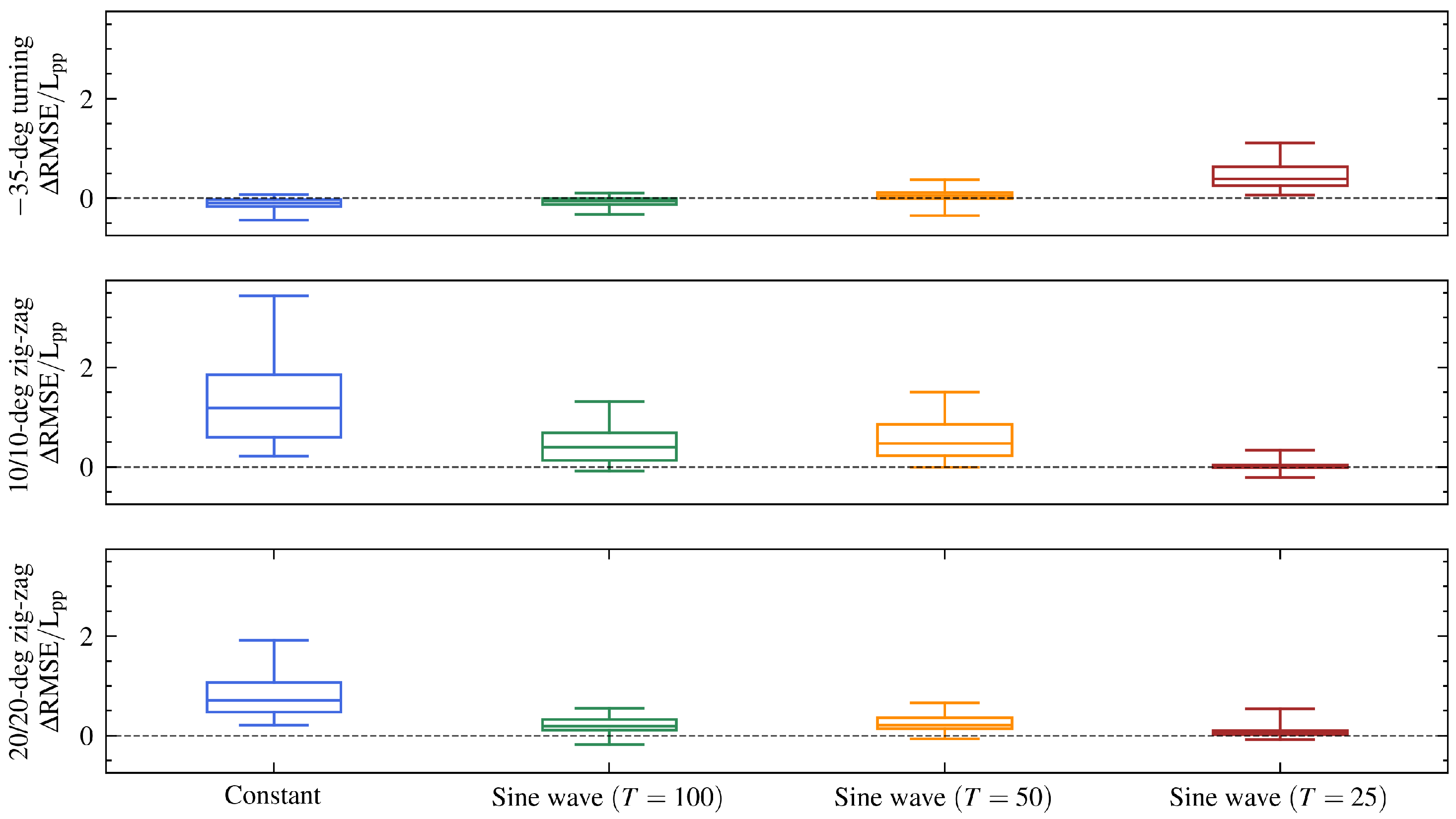
To further clarify the relative superiority of the excitation signals on a per-realization basis, Figure 8 presents boxplots of the differences in median RMSE () between the linearly decreasing signal and the other candidate signals. The difference is defined as such that a positive value indicates that the linearly decreasing signal achieved a smaller prediction error. The majority of the values lie in the positive region, particularly against the 25-s-period sinusoidal signal in the turning maneuver and against the constant and longer-period sinusoidal signals in the zig-zag maneuvers. This confirms that the linearly decreasing signal provides a consistent reduction in prediction error across various noise conditions. Overall, this repeated-realization analysis robustly supports the conclusion of this section that the linearly decreasing signal yields the most balanced and reliable predictive performance among the candidates.
Figure 8.
Boxplots of the differences in the median of the non-dimensionalized RMSEs between the linearly decreasing signal and the other candidate signals. The dotted liines indicare zero.
In addition to the turning and zig-zag tests, the course stability of the identified models was further investigated via spiral test simulations. The detailed results are presented in Appendix B.
4.2. Hydrodynamic Coefficient Identification Using Pseudo-Observation Data Generated from the Perturbed Rudder Profile
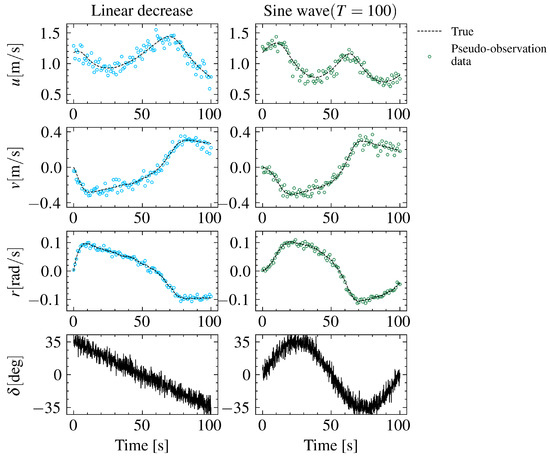
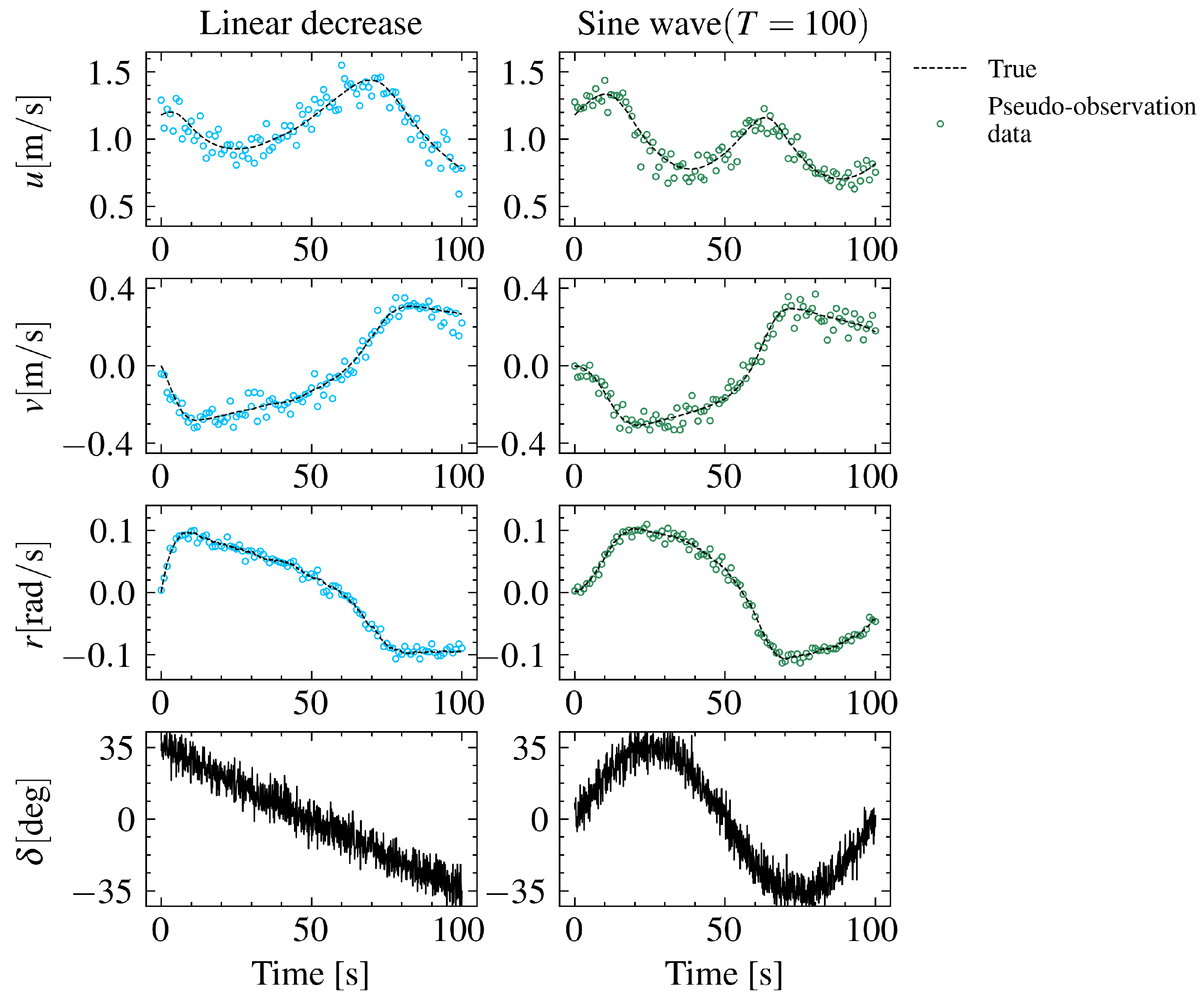
The sensitivity of the identification results to a specific synthetic input perturbation is further examined by introducing deviations between the commanded and actual rudder angles. The analysis focuses on the linearly decreasing signal and the 100-s-period sinusoidal signal because these produced the most balanced predictive performance among the cases examined in Section 4.1. Figure 9 displays the pseudo-observation data and the actual rudder angle variation. The black dashed lines represent the true values of each velocity component. As previously detailed in Section 3.2, the rudder angle employed for identifying the hydrodynamic coefficients does not correspond to the actual rudder angle depicted in Figure 9. Instead, the ideal commanded rudder angle as in Equation (6) is employed for the identification process.
Figure 9.
Pseudo-observation data and time series of the rudder angle.
Table 4 summarizes the sampling diagnostics for the two synthetically perturbed-input cases. For the two synthetically perturbed-input cases, the largest value was 1.007, while the minimum bulk and tail ESS values were 1531 and 1702, respectively. No divergent transitions or transitions reaching the maximum tree depth were observed. These diagnostics indicate satisfactory mixing and numerical convergence of the four chains. The corresponding trace plots are presented in Appendix A.
Table 4.
MCMC sampling diagnostics for the synthetically perturbed-input cases. The maximum and the minimum bulk and tail ESS were calculated over all 20 inferred parameters.
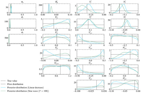
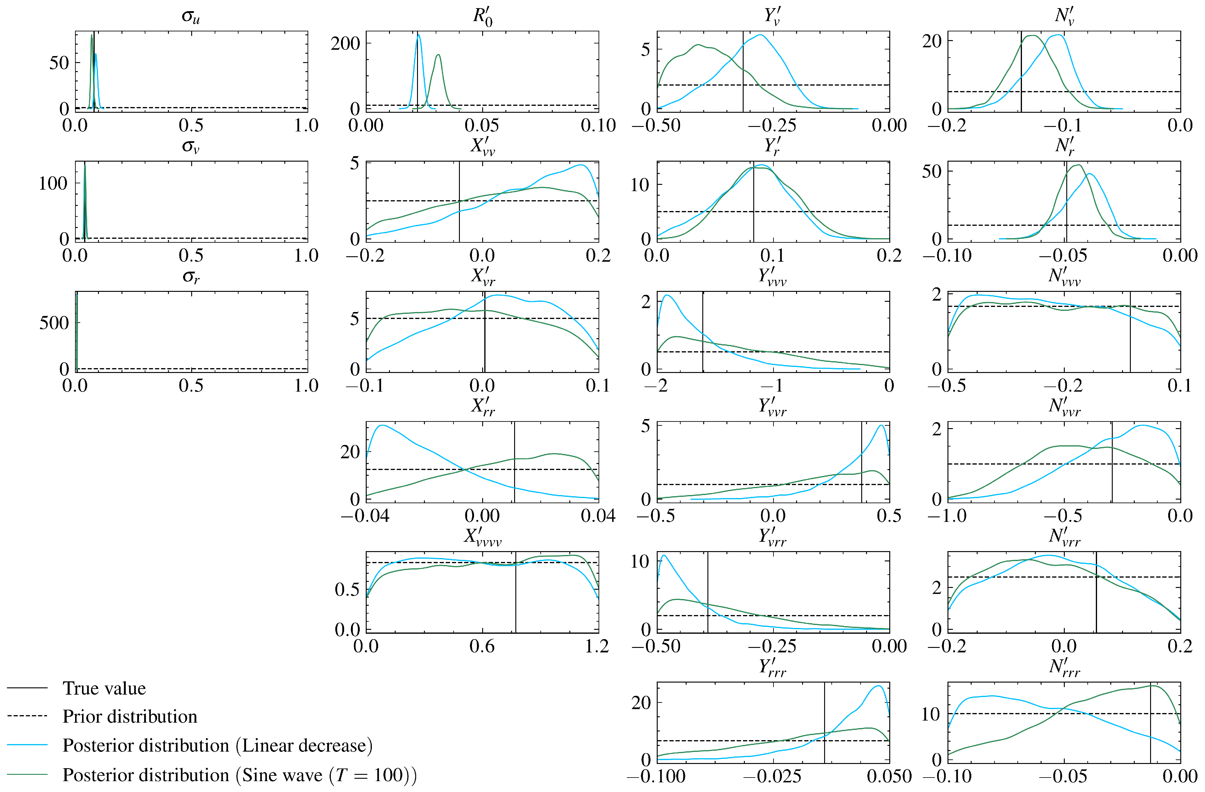
Figure 10 shows the prior and posterior probability distributions of hydrodynamic coefficients and observation-noise standard deviations identified from these pseudo-observation data. The vertical black line, black dashed line, and colored lines represent the true value, the prior distribution, and the posterior distribution of each parameter, respectively. A visual comparison with the posterior distributions shown in Figure 2 reveals no substantial overall deterioration for the two tested signals. This result indicates that, in the present numerical case study, the posterior distributions were not highly sensitive to the particular synthetic rudder-angle perturbation considered here.
Figure 10.
Prior and posterior distributions of hydrodynamic coefficients and observation-noise standard deviations.
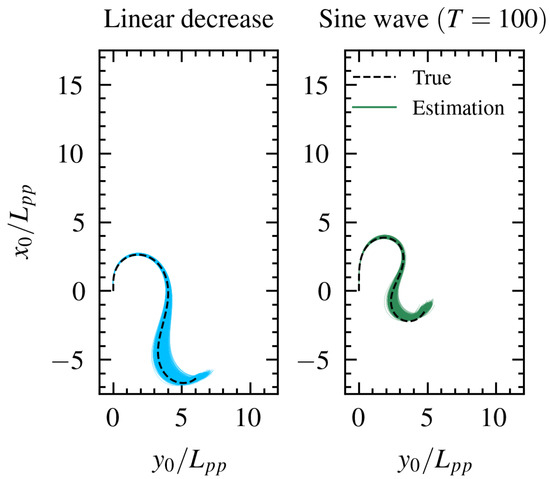
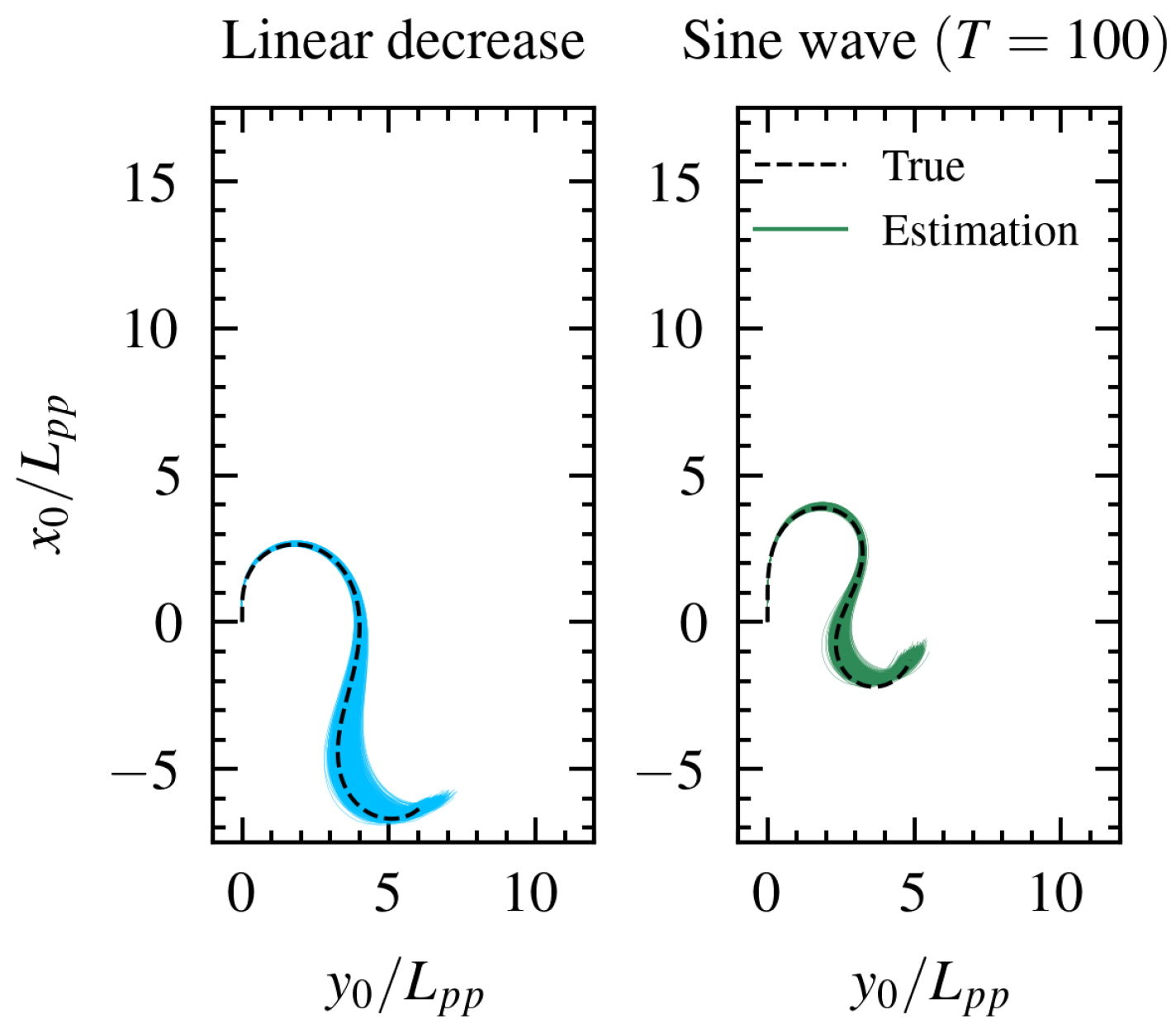
Subsequently, it is verified that MMG models containing these samples of hydrodynamic coefficients can reproduce the maneuvering motions used for the identification, given that the ideal excitation signals are different from the actual rudder angle variations. Four thousand MMG models, each corresponding to one of the 4000 samples of hydrodynamic coefficients, are used for estimation. Figure 11 shows the true and estimated trajectories. In both cases, the MMG models accurately reproduce the maneuvering motions used for identification regardless of the presence of the synthetic rudder angle perterbation.
Figure 11.
Estimated trajectories under each candidate rudder input using the identified models.
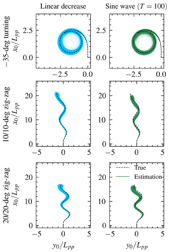
Finally, the cross-maneuver predictive performance is evaluated using the same held-out rudder-input histories as in Section 4.1. Figure 12 shows the prediction results of the three standard tests using 4000 MMG models obtained from each maneuvering dataset. Figure 13 presents boxplots of RMSEs between the true and estimated trajectories. The definition of whiskers, the upper and lower edges, and the line inside the box is the same as in red. A comparison of these figures with Figure 5 and Figure 6 reveals that no substantial deterioration in predictive performance was observed. These results indicate that, for the synthetic perturbation examined here, the predictive performance of the identified models was not substantially degraded. Further evaluation using actuator dynamics and experimental or full-scale data is required before the applicability of these signals to practical operations can be established.
Figure 12.
Predicted trajectories of -35-deg turning, 10/10-deg zig-zag, and 20/20-deg zig-zag.
Figure 13.
Boxplots of non-dimensionalized RMSEs between the true and predicted trajectories.
5. Discussion
In this numerical case study, the linearly decreasing input produced the most balanced predictive performance across the held-out maneuvers. A plausible explanation for this result is that the input generated a continuous transition from turning motion to approximately straight-line motion and then toward turning in the opposite direction within the 100-s observation period. In contrast, the constant input rapidly approached a steady turning condition, while the ship response to the shorter-period sinusoidal inputs was attenuated because of the relatively slow maneuvering dynamics. These differences resulted in distinct motion histories being available for parameter identification. However, a constant rudder-angle rate does not by itself establish that the maneuvering dynamics are uniformly excited over the entire rudder-angle range. Because only one rate of linear rudder-angle variation was examined, the relationship between the ramp rate, the ship response time scale, and identification performance remains to be investigated.
Within the Bayesian inference framework employed in this study, posterior contraction relative to the prior indication provides a prior-dependent indication of parameter identifiability for each parameter. When excitation inputs with low identifiability are utilized, the resulting posterior distributions show limited updates from their prior distributions. This indicates that the observation data lack sufficient information to explicitly pinpoint the parameters. Consequently, this uncertainty manifests as larger variance in the estimated trajectories. For the linearly decreasing input, several hydrodynamic coefficients exhibited clearer concentration in their posterior distributions than for the constant input. These results indicate that, among the candidate inputs examined in this study, the linearly decreasing input provided a favorable balance between parameter uncertainty and predictive performance across the tested maneuvers.
The effectiveness of the excitation signals can be further understood from the perspective of how the input shapes the posterior distribution through the likelihood function. Since the likelihood is constructed based on the discrepancy between the model response and the observation data generated by a given input signal, the choice of excitation input directly influences the structure of the likelihood function and, consequently, the resulting posterior distribution. Excitation inputs that induce limited or repetitive motion patterns, such as constant rudder inputs, may result in broader likelihood regions, allowing a wide range of parameter values to explain the data. This leads to posterior distributions that remain broadly spread and close to the prior. In contrast, excitation inputs that generate diverse maneuvering responses may produce more concentrated likelihood regions, which more effectively constrain the parameter space and result in more concentrated posterior distributions. This perspective provides a unified interpretation of the observed differences in identifiability across excitation signals, linking the characteristics of excitation signals to parameter identifiability through the Bayesian inference framework.
A more detailed interpretation can be obtained by examining not only the presence of distinct posterior peaks but also the spread of the posterior distributions across different excitation inputs. For lower-order hydrodynamic coefficients, the posterior distributions obtained from sinusoidal excitation tend to exhibit narrower spreads compared to those from constant and linearly decreasing inputs. This indicates that sinusoidal inputs can effectively constrain certain low-order parameters due to their periodic excitation characteristics. In contrast, for higher-order hydrodynamic coefficients, the linearly decreasing input occasionally results in relatively narrower posterior distributions compared to other excitation signals. However, the reduction in uncertainty is less pronounced than that observed for lower-order coefficients, and the differences among excitation signals remain limited. This suggests that the identifiability of higher-order coefficients is likely restricted by correlations among the polynomial terms representing the hydrodynamic forces acting on the ship hull, rather than being solely determined by the choice of excitation signal. From the perspective of system identification, such potential correlations in the model structure are undesirable. Consequently, the model may necessitate simplification or modification of the polynomial.
This study is limited to a numerical case study using a single KVLCC2 model under a normal forward-speed condition. The model structure and all parameters other than the identified hydrodynamic coefficients were assumed to be known, and the training and evaluation data were generated using the same MMG formulation. In addition, only one duration and one ramp rate were considered for the linearly decreasing input, and the rudder-angle deviations were represented by a synthetic perturbation rather than by an actuator model. Therefore, the present results should be interpreted as a comparison of predictive performance among the tested input signals, rather than as evidence of general applicability to different ships or full-scale operations. Future work should examine multiple ship types, input durations, ramp rates, noise realizations, and experimentally measured rudder responses.
6. Conclusions
This study comparatively examined excitation signals to obtain observation data suitable for identifying parameters of ship maneuvering models. Based on considerations of system identification, maneuvering response, and operational feasibility, rudder-angle range, temporal variation, and the ship response time scale were adopted as criteria for comparing the candidate excitation signals. In order to evaluate the effectiveness of excitation signals that meet the requirements, the hydrodynamic coefficients of the MMG model of the KVLCC2 model ship were identified using pseudo-observation data. Under idealized conditions where the same MMG formulation was used for both data generation and identification, the pseudo-observation data were generated using the following candidate excitation signals: a constant maximum rudder angle, a linearly decreasing rudder angle between the positive and negative maximum limits, and sinusoidal variations with the maximum rudder angle as their amplitudes. A Bayesian inference framework using the MCMC-based method [24] was employed to quantify parameter uncertainty while explicitly accounting for observation noise. The cross-maneuver predictive performance of the identified MMG models was evaluated using held-out rudder-input histories obtained from turning and zig-zag simulations. In the present numerical case study, the linearly decreasing input generated a motion history containing transitions between turning and approximately straight-line behavior. Among the tested cases, the models identified using the linearly decreasing input produced the relatively small and balanced trajectory errors across the held-out turning and zig-zag maneuvers. The results also suggest that rudder-angle coverage alone may be insufficient and that the time scale of input variation relative to the ship response should be considered. However, this study did not systematically examine the effect of the ramp rate. For the specific synthetic rudder-angle perturbation examined here, the identified models retained predictive performance broadly similar to that obtained in the ideal-input cases. These results support the further evaluation of simple, structured rudder-angle signals, particularly the linearly decreasing signal, as candidates for acquiring informative data for MMG model identification.
Author Contributions
Conceptualization, S.G., T.M. and H.S.; methodology, S.G. and H.S.; software, S.G. and K.H.; investigation, S.G., H.S. and K.H.; data curation, K.H.; writing—original draft preparation, S.G.; writing—review and editing, T.M. and H.S.; visualization, S.G.; supervision, T.M. All authors have read and agreed to the published version of the manuscript.
Funding
This work was partially supported by JST SPRING, Grant Number JPMJSP2178, JSPS KAKENHI, Grant Number 24K07902, and Fundamental Research Developing Association for Shipbuilding and Offshore (REDAS).
Data Availability Statement
The original contributions presented in this study are included in the article. Further inquiries can be directed to the corresponding authors.
Conflicts of Interest
Author Hyuga Shimozawa was employed by MTI Co., Ltd, Tokyo. The remaining authors declare that the research was conducted in the absence of any commercial or financial relationships that could be construed as potential conflicts of interest.
Appendix A. Trace Plots of MCMC Samples
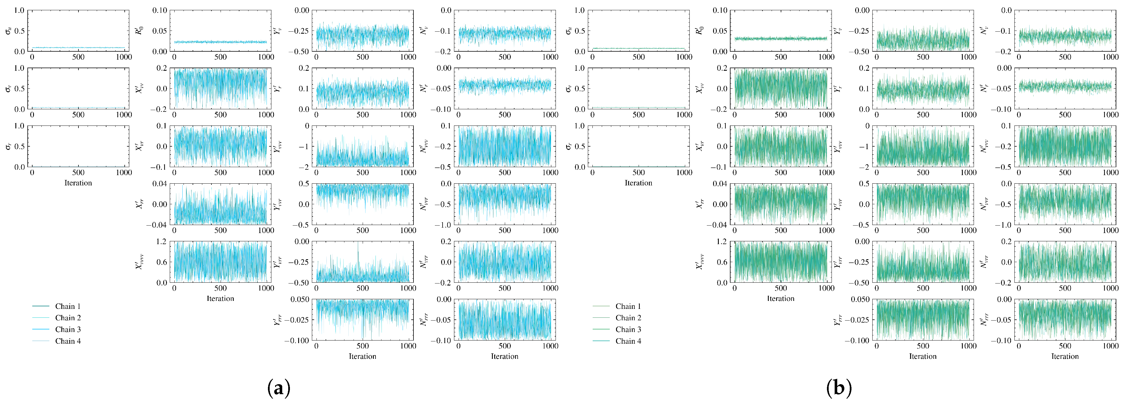
Figure A1 and Figure A2 show the trace plots of post-warmup MCMC samples in Section 4.1 and Section 4.2, respectively. The vertical axis limits correspond to the prior distribution ranges of each standard deviation and hydrodynamic coefficient. The trace plots show random fluctuations around a constant mean within a well-defined bound, confirming the stationarity of the chains and indicating that the numbers of warmup steps and collected samples are sufficient for the parameter identification. Visual inspection revealed no persistent trends or chain-specific separation. Quantitative convergence diagnostics for all 20 inferred parameters are reported in Table 2 and Table 4.
Figure A1.
Trace plots of the four post-warmup NUTS chains for the ideal-input cases in Section 4.1: (a) constant rudder angle; (b) linearly decreasing rudder angle; (c) sinusoidal rudder angle with s; (d) sinusoidal rudder angle with s; and (e) sinusoidal rudder angle with s.
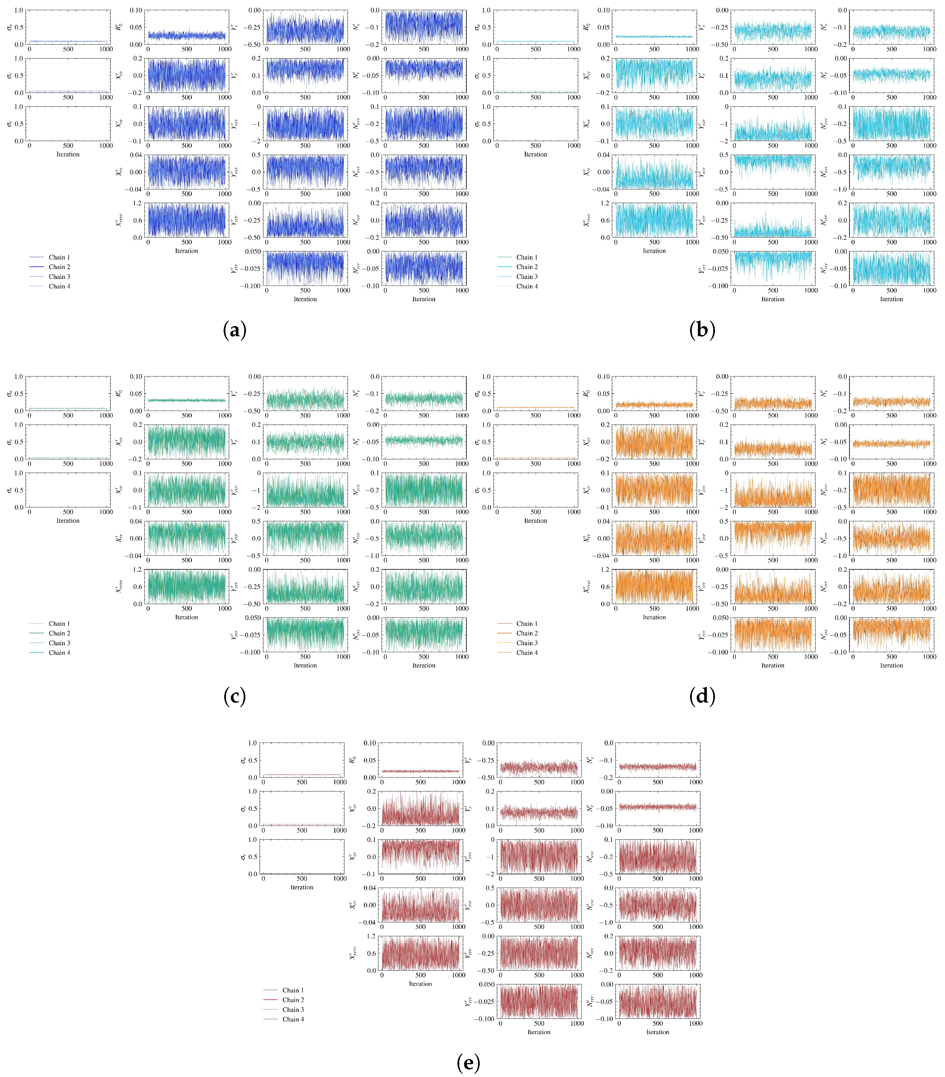
Figure A2.
Trace plots of the four post-warmup NUTS chains for the synthetically perturbed-input cases in Section 4.2: (a) linearly decreasing rudder angle; and (b) sinusoidal rudder angle with s.
Appendix B. Spiral Test Results
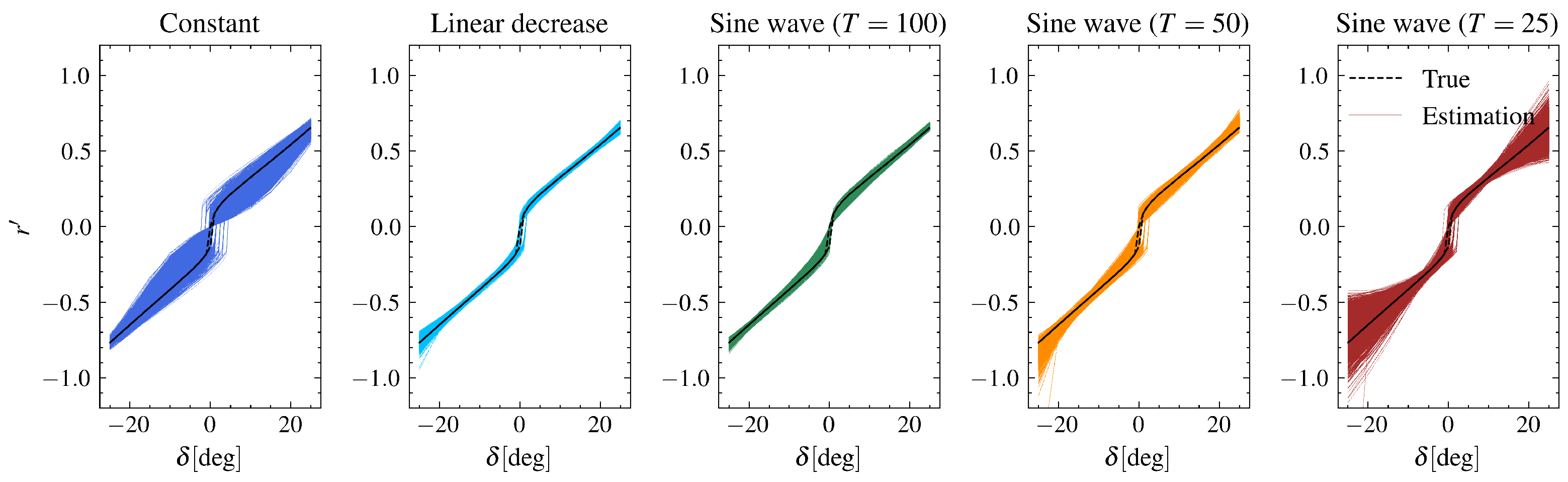
To evaluate course stability of the identified models, direct spiral test simulations were conducted using the 4000 MMG models obtained from each maneuvering dataset in Section 4.1. In the simulation procedure, the rudder angle was step-wise varied in a continuous sweep from to degrees and then back to degrees, with 5-degree increments for and finer 1-degree increments within the range of . At each step, the simulation was executed until the ship motions strictly reached a steady state. Specifically, a steady state was determined when the sliding-window variations of the velocity components () over a 30-s duration remained below for three consecutive seconds, with a maximum time limit of 1000 s per rudder step. The final state variables at each step were continuously passed as the initial conditions for the subsequent rudder angle to correctly capture the dynamic hysteresis loop. Although the simulations were evaluated at discrete rudder angle increments, the resulting spiral curves are presented with piecewise linear interpolation for clarity and in accordance with standard conventions.
Figure A3 illustrates the resulting spiral curves for each maneuvering dataset. The colored lines represent the spiral curves generated by the 4000 MMG models, and the dashed black lines indicate the true spiral curve derived from the true MMG model. As shown in the figure, the linearly decreasing signal and the 100-s-period sinusoidal input, effectively capture the true hysteresis loop with narrow uncertainty bounds. In contrast, the models identified from the other maneuvers show larger discrepancies, highlighting the importance of informative training data for accurate course stability assessment.
Figure A3.
Spiral test results using the identified MMG models obtained from each maneuvering datasets in Section 4.1.
References
- Maki, A.; Sakamoto, N.; Akimoto, Y.; Nishikawa, H.; Umeda, N. Application of optimal control theory based on the evolution strategy (CMA-ES) to automatic berthing. J. Mar. Sci. Technol. 2020, 25, 221–233. [Google Scholar] [CrossRef] [Scilit]
- Kang, Y.T.; Chen, W.J.; Zhu, D.Q.; Wang, J.H. Collision avoidance path planning in multi-ship encounter situations. J. Mar. Sci. Technol. 2021, 26, 1026–1037. [Google Scholar] [CrossRef] [Scilit]
- Sawada, R.; Sato, K.; Majima, T. Automatic ship collision avoidance using deep reinforcement learning with LSTM in continuous action spaces. J. Mar. Sci. Technol. 2021, 26, 509–524. [Google Scholar] [CrossRef] [Scilit]
- Miyauchi, Y.; Sawada, R.; Akimoto, Y.; Umeda, N.; Maki, A. Optimization on planning of trajectory and control of autonomous berthing and unberthing for the realistic port geometry. Ocean Eng. 2022, 245, 110390. [Google Scholar] [CrossRef] [Scilit]
- Abkowitz, M.A. Lectures on Ship Hydrodynamics-Steering and Manoeuvrability; Report No. Hy-5; Hydro- and Aerodynamics Laboratory: Lyngby, Denmark, 1964. [Google Scholar]
- Fossen, T.I. Guidance and Control of Ocean Vehicles, reprint ed.; Wiley: Chichester, UK, 1999. [Google Scholar]
- Yasukawa, H.; Yoshimura, Y. Introduction of MMG standard method for ship maneuvering predictions. J. Mar. Sci. Technol. 2015, 20, 37–52. [Google Scholar] [CrossRef] [Scilit]
- Moreira, L.; Guedes Soares, C. Dynamic model of manoeuvrability using recursive neural networks. Ocean Eng. 2003, 30, 1669–1697. [Google Scholar] [CrossRef] [Scilit]
- Rajesh, G.; Bhattacharyya, S. System identification for nonlinear maneuvering of large tankers using artificial neural network. Appl. Ocean Res. 2008, 30, 256–263. [Google Scholar] [CrossRef] [Scilit]
- Zhang, X.G.; Zou, Z.J. Black-box modeling of ship manoeuvring motion based on feed-forward neural network with Chebyshev orthogonal basis function. J. Mar. Sci. Technol. 2013, 18, 42–49. [Google Scholar] [CrossRef] [Scilit]
- Jiang, Y.; Hou, X.R.; Wang, X.G.; Wang, Z.H.; Yang, Z.L.; Zou, Z.J. Identification modeling and prediction of ship maneuvering motion based on LSTM deep neural network. J. Mar. Sci. Technol. 2022, 27, 125–137. [Google Scholar] [CrossRef] [Scilit]
- Wang, Z.; Kim, J.; Im, N. Non-parameterized ship maneuvering model of Deep Neural Networks based on real voyage data-driven. Ocean Eng. 2023, 284, 115162. [Google Scholar] [CrossRef] [Scilit]
- Wang, X.g.; Zou, Z.j.; Hou, X.r.; Xu, F. System identification modelling of ship manoeuvring motion based on ε-support vector regression. J. Hydrodyn. 2015, 27, 502–512. [Google Scholar] [CrossRef] [Scilit]
- Wang, Z.; Xu, H.; Xia, L.; Zou, Z.; Soares, C.G. Kernel-based support vector regression for nonparametric modeling of ship maneuvering motion. Ocean Eng. 2020, 216, 107994. [Google Scholar] [CrossRef] [Scilit]
- Ramirez, W.A.; Leong, Z.Q.; Nguyen, H.; Jayasinghe, S.G. Non-parametric dynamic system identification of ships using multi-output Gaussian Processes. Ocean Eng. 2018, 166, 26–36. [Google Scholar] [CrossRef] [Scilit]
- Xue, Y.; Liu, Y.; Ji, C.; Xue, G.; Huang, S. System identification of ship dynamic model based on Gaussian process regression with input noise. Ocean Eng. 2020, 216, 107862. [Google Scholar] [CrossRef] [Scilit]
- Ueno, M.; Yoshimura, Y.; Tsukada, Y.; Miyazaki, H. Circular motion tests and uncertainty analysis for ship maneuverability. J. Mar. Sci. Technol. 2009, 14, 469–484. [Google Scholar] [CrossRef] [Scilit]
- Shenoi, R.R.; Krishnankutty, P.; Panneer Selvam, R. Study of manoeuvrability of container ship by static and dynamic simulations using a RANSE-based solver. Ships Offshore Struct. 2016, 11, 316–334. [Google Scholar] [CrossRef] [Scilit]
- Guo, H.p.; Zou, Z.j. System-based investigation on 4-DOF ship maneuvering with hydrodynamic derivatives determined by RANS simulation of captive model tests. Appl. Ocean Res. 2017, 68, 11–25. [Google Scholar] [CrossRef] [Scilit]
- Åström, K.J.; Källström, C.G. Identification of ship steering dynamics. Automatica 1976, 12, 9–22. [Google Scholar] [CrossRef] [Scilit]
- Yoon, H.K.; Rhee, K.P. Identification of hydrodynamic coefficients in ship maneuvering equations of motion by Estimation-Before-Modeling technique. Ocean Eng. 2003, 30, 2379–2404. [Google Scholar] [CrossRef] [Scilit]
- Miyauchi, Y.; Maki, A.; Umeda, N.; Rachman, D.M.; Akimoto, Y. System parameter exploration of ship maneuvering model for automatic docking/berthing using CMA-ES. J. Mar. Sci. Technol. 2022, 27, 1065–1083. [Google Scholar] [CrossRef] [Scilit]
- Xue, Y.; Liu, Y.; Ji, C.; Xue, G. Hydrodynamic parameter identification for ship manoeuvring mathematical models using a Bayesian approach. Ocean Eng. 2020, 195, 106612. [Google Scholar] [CrossRef] [Scilit]
- Mitsuyuki, T.; Kuribayashi, K.; Fernandez, R.F.S.; Shimozawa, H.; Kakuta, R.; Niki, R.; Matsushita, R. MMG 3DOF model identification with uncertainty of observation and hydrodynamic maneuvering coefficients using MCMC method. J. Mar. Sci. Technol. 2024, 29, 668–682. [Google Scholar] [CrossRef] [Scilit]
- Nouri, N.M.; Valadi, M.; Asgharian, J. Optimal input design for hydrodynamic derivatives estimation of nonlinear dynamic model of AUV. Nonlinear Dyn. 2018, 92, 139–151. [Google Scholar] [CrossRef] [Scilit]
- Wang, Z.; Guedes Soares, C.; Zou, Z. Optimal design of excitation signal for identification of nonlinear ship manoeuvring model. Ocean Eng. 2020, 196, 106778. [Google Scholar] [CrossRef] [Scilit]
- Andrieu, C.; de Freitas, N.; Doucet, A.; Jordan, M.I. An Introduction to MCMC for Machine Learning. Mach. Learn. 2003, 50, 5–43. [Google Scholar] [CrossRef] [Scilit]
- Yoshimura, Y.; Nakamura, M.; Taniguchi, T.; Yasukawa, H. Empirical formulas of hydrodynamic parameters for predicting ship maneuvering based on the MMG-model. Ocean Eng. 2025, 337, 121831. [Google Scholar] [CrossRef] [Scilit]
- Homan, M.D.; Gelman, A. The No-U-turn sampler: Adaptively setting path lengths in Hamiltonian Monte Carlo. J. Mach. Learn. Res. 2014, 15, 1593–1623. [Google Scholar]
- Ge, H.; Xu, K.; Ghahramani, Z. Turing: A Language for Flexible Probabilistic Inference. In Proceedings of the Twenty-First International Conference on Artificial Intelligence and Statistics, Lanzarote, Spain, 9–11 April 2018; pp. 1682–1690. [Google Scholar]
- Ishiguro, T.; Tanaka, S.; Yoshimura, Y. A study on the accuracy of the recent prediction technique of ship’s manoeuvrability at early design stage. In Marine Simulation and Ship Manoeuvrability, 1st ed.; Routledge: London, UK, 1996; pp. 547–561. [Google Scholar] [CrossRef] [Scilit]

Disclaimer/Publisher’s Note: The statements, opinions and data contained in all publications are solely those of the individual author(s) and contributor(s) and not of MDPI and/or the editor(s). MDPI and/or the editor(s) disclaim responsibility for any injury to people or property resulting from any ideas, methods, instructions or products referred to in the content. |
© 2026 by the authors. Licensee MDPI, Basel, Switzerland. This article is an open access article distributed under the terms and conditions of the Creative Commons Attribution (CC BY) license.