


Abstract
The exhaust gas temperature (EGT) of marine diesel engines is an important parameter reflecting the engine’s operating conditions. Its variation is influenced by complex thermodynamic processes, including combustion fluctuations and thermal inertia effects, and exhibits significant non-stationarity and multiscale fluctuation characteristics, posing considerable challenges for multi-step forecasting. To address this issue, this paper proposes a multi-step EGT forecasting method for marine diesel engines based on frequency-aware trend-residual learning. This method first extracts long-term variation information from the EGT sequence, then employs frequency-domain analysis to enhance and characterize short-term fluctuation components, and applies temporal feature learning with an adaptive fusion strategy to effectively integrate information across different time scales, thereby improving the accuracy of multi-step EGT forecasting. Based on actual ship operation data, multi-step EGT forecasting tasks with different horizons are established, and the proposed method is compared with several typical deep learning models. Experimental results show that the proposed method achieves competitive and consistent performance across all forecasting horizons. For one-step to four-step forecasting tasks, the mean absolute errors are 0.3078, 0.5037, 0.6835 and 0.8312, respectively, all of which are lower than those of the comparison models. Moreover, the proposed method demonstrates stable performance in evaluation metrics such as mean squared error. These results verify the effectiveness of the proposed method.
1. Introduction
Global maritime transport constitutes the backbone of international trade, accounting for over 80% of global trade by volume. The operational efficiency and safety of ships exert a profound influence on the stability of the global maritime transportation system [1,2]. In recent years, driven by the rapid advancement of maritime digitalization and intelligent technologies, the volume of operational data generated onboard has grown exponentially, establishing a robust foundation for the deployment of data-driven methodologies in marine power systems. Condition monitoring based on operational data has become an important research direction in intelligent ship operation and maintenance [2,3].
As the primary propulsion unit of ocean-going ships, marine diesel engines typically operate continuously for prolonged periods. Due to the combined effects of combustion, scavenging, and heat transfer processes, their operating parameters exhibit distinctly nonlinear and non-stationary characteristics [3,4,5,6]. Under the mutual influence of multiple variables, complex temporal dependencies exist among these operating parameters, increasing the difficulty of analyzing and predicting engine operating conditions. Exhaust gas temperature (EGT) is a critical thermodynamic parameter reflecting the operating condition of diesel engines. It effectively characterizes essential operational information such as combustion efficiency and intake air supply conditions, and has thus been widely referenced in the literature for engine health monitoring and diagnostic analysis [7,8,9,10]. Variations in EGT are comprehensively governed by the combustion heat release, intake, and exhaust processes, and energy conversion within the turbocharger. Furthermore, this thermal response is mediated by the thermal inertia of the system, resulting in a certain delay when responding to changes in operating conditions [6,11,12]. These underlying physical mechanisms cause the EGT sequence to exhibit both long-term variations and short-term fluctuations, while complex interdependencies also exist among variables, thereby increasing the difficulty of the forecasting task [5].
With the growing intelligence of ships, the demand for future state information in operational decision-making is rising. Single-step prediction provides limited information and is thus insufficient to meet the practical requirements of continuous condition monitoring and trend analysis. Compared to single-step methods, multi-step forecasting can provide information about future state evolution over longer forecasting horizons, better satisfying the requirements of ship power system monitoring and decision support [11,12,13]. However, the EGT sequence exhibits significant non-stationarity and intricate temporal dependencies due to the underlying thermodynamic interactions of combustion and heat transfer. With the expansion of the forecasting horizon, prediction errors tend to accumulate gradually. Simultaneously, existing models struggle to effectively separate long-term trend information from short-term fluctuation information embedded in the sequence and jointly exploit them, resulting in a further decline in multi-step forecasting accuracy. Consequently, capturing intricate temporal patterns alongside variable interdependencies remains challenging. Furthermore, effectively synergizing multi-scale sequence components to mitigate error propagation constitutes a critical bottleneck in multi-step EGT forecasting for marine diesel engines.
To tackle the challenges of time series forecasting, various data-driven methods have been proposed in previous studies. Early studies predominantly relied on statistical learning and traditional machine learning techniques, which mapped inputs to outputs but suffered from a limited capacity to model complex, highly nonlinear temporal dependencies [14]. Subsequently, recurrent neural networks (RNNs) and their variants have been widely adopted to leverage historical information via recursive hidden states [15]. Nonetheless, in long-horizon forecasting tasks, recurrent structures inherently cause severe error accumulation, leading to rapid performance degradation as the forecasting horizon increases [16]. In recent years, Transformer-based architectures have emerged as the mainstream paradigm for multi-step forecasting, owing to their superior ability to capture long-range temporal dependencies. For instance, Informer mitigates the quadratic computational complexity of long-sequence forecasting by introducing a sparse attention mechanism [13]. Autoformer enhances the representation capability for non-stationary sequences through a series decomposition strategy [17]. Expanding on this, the Frequency Enhanced Decomposed Transformer (FEDformer) integrates frequency-domain analysis to capture global patterns in the compact spectral space, significantly improving long-term forecasting accuracy [18]. Furthermore, some studies have proposed task-specific approaches for different types of time series. The Decomposition Linear model (DLinear) delivers high-efficiency forecasting by coupling basic series decomposition with direct linear mapping [19]; the Patch Time Series Transformer (PatchTST) employs a patch-based learning strategy to enhance the representation of local temporal features [20]. Inverted transformers (iTransformer) improves multivariate time series representation by rethinking the role of variables and reorganizing the dimension structure [21]. With the development of foundation models for time series, unified representation learning and large-scale pretraining have further expanded their application potential across various tasks [22]. Collectively, existing methods have made notable progress in long-term dependency learning and non-stationary sequence processing. However, effective integration of long-term and short-term information components, as well as the mitigation of error accumulation in multi-step forecasting, remain insufficiently explored.
Although general time-series forecasting models have achieved considerable progress, marine diesel engine EGT forecasting remains a highly task-specific problem due to the strong coupling between thermal processes and operational conditions. Previous studies on marine engine condition monitoring have mainly focused on EGT prediction, performance estimation, and fault-related analysis using statistical models, machine learning approaches, or deep neural networks [10,23]. These studies demonstrated the feasibility of data-driven methods for capturing nonlinear relationships between EGT and engine operating parameters, such as engine speed, fuel-related variables, and air supply conditions [24].
However, existing marine-engine EGT forecasting studies still face several limitations. First, many existing approaches mainly focus on one-step prediction or short-term regression tasks, while multi-step forecasting with accumulated prediction errors has received relatively limited attention. Second, EGT variations are jointly determined by slow thermal response characteristics and rapid transient disturbances, whereas previous methods generally model the temperature sequence as a unified signal without explicitly separating different temporal components. Third, although multiple engine parameters exhibit complex coupling relationships, variable dependencies are commonly modeled using fixed correlation assumptions, which may not fully represent dynamic interactions during changing operating conditions. These limitations indicate that an effective marine-engine EGT forecasting model should simultaneously consider multi-scale thermal evolution, transient fluctuation characteristics, and dynamic dependencies among operating variables.
In addition to temporal dependencies, dependency information among multiple variables is also an important factor influencing predictive performance. To address this issue, graph neural networks (GNNs) have gradually been applied to multivariate time series forecasting by using graph structures to model dependencies among variables. Graph WaveNet utilizes an adaptive adjacency matrix to learn implicit dependencies among variables [25], and multivariate time series graph neural networks (MTGNN) further enhances graph structure learning capability, improving the representation of multivariate relationships [26]. In recent years, some studies have explored representation methods that incorporate dynamic graph structures or domain knowledge to further improve predictive performance in complex systems. For instance, ForecastGrapher enhances the representation of variable relationships through time-varying graph structures [27]. Chen et al. introduced thermodynamic priors into a graph attention network for engine EGT prediction, verifying the effectiveness of integrating physical priors with graph structures [28].
Although existing studies have improved forecasting performance in terms of temporal dependency learning, non-stationary sequence modeling, and variable relationship representation, limitations still remain in marine diesel engine EGT forecasting. On the one hand, prediction errors tend to accumulate as the forecasting horizon increases, and multi-scale information components are not systematically and jointly exploited. On the other hand, most multivariate relationships are modeled using static relationship assumptions or fixed structures, and time-varying dependencies among variables are not fully exploited. Therefore, effectively exploiting long-term variation information, short-term fluctuation information, and time-varying statistical dependencies among variables to improve the stability and accuracy of multi-step EGT forecasting remains an important research direction.
However, directly applying existing forecasting architectures to marine diesel engine EGT prediction remains challenging because the temporal characteristics of EGT are closely associated with the underlying thermodynamic processes of the engine. Specifically, the long-term evolution of EGT is dominated by thermal inertia and gradual changes in operating conditions, whereas short-term fluctuations are influenced by transient combustion variations, fuel supply disturbances, and turbocharging dynamics. Meanwhile, the interactions among monitored variables exhibit dynamic coupling relationships that cannot be fully characterized by fixed dependency assumptions.
Therefore, the primary objective of this study is to develop a task-oriented framework that integrates multiple representation strategies tailored to the characteristics of marine diesel engine operation, rather than introducing isolated model components. Such a framework should simultaneously account for low-frequency thermal evolution, high-frequency transient fluctuations, and dynamic dependencies among operating variables, thereby enhancing the capability of multi-step EGT prediction.
To address these aforementioned challenges, this paper proposes a frequency-aware trend-residual graph neural network, termed FTRG-Net, for the multi-step EGT forecasting of marine diesel engines. This framework focuses on the effective integration of trend and residual information. Specifically, the framework decomposes the historical multivariate sequence into multi-scale trend and residual components; the low-frequency macro-trends are fitted via a multi-scale linear mapping branch. Concurrently, within the residual branch, a frequency-aware extraction mechanism maps the temporal residuals to the spectral domain, isolating and amplifying high-frequency fluctuation components via differentiable filtering; these enhanced high-frequency components are subsequently learned by a Modern Temporal Convolutional Network (ModernTCN) block to capture localized dynamic fluctuations. To reconstruct dynamic inter-variable relationships, FTRG-Net introduces an adaptive graph-fusion residual learning module. This module estimates a statistical prior graph via sliding-window mutual information (MI) to describe explicit correlations, while simultaneously generating a data-driven learnable adjacency matrix to uncover latent implicit dependencies. By dynamically blending these dual graphs using a gating-derived fusion coefficient, the spatial features are propagated through graph convolutions to yield highly discriminative multivariate representations. Ultimately, an adaptive fusion mechanism is developed to coordinate temporal and graph-based features, while a gating strategy is introduced to adjust the contribution of residual information to trend refinement. This enables the effective integration of different information components.
The major contributions of this paper are summarized as follows:
- (1)
- A task-oriented frequency-aware trend-residual forecasting framework is proposed for multi-step marine diesel engine EGT prediction. Different from directly applying general time-series forecasting models, the proposed framework explicitly separates low-frequency thermal evolution and high-frequency transient fluctuations according to the dynamic characteristics of marine engine operation.
- (2)
- An adaptive dependency learning strategy is developed by integrating mutual-information-based statistical relationships and learnable graph structures. This design enables the model to simultaneously exploit explicit operating-condition correlations and hidden nonlinear dependencies among engine variables.
- (3)
- Extensive experiments based on real ship operational data are conducted to evaluate the effectiveness and robustness of the proposed method under different forecasting horizons. The results demonstrate the effectiveness of jointly modeling temporal-scale information and variable dependencies for marine engine condition monitoring.
The structure of this paper is organized as follows. Section 2 presents the overall framework of the proposed method, including the trend decomposition module, the frequency-aware residual module, the graph neural network module, and the design of the fusion mechanism. Section 3 provides the experimental design and implementation details, covering data sources, preprocessing methods, comparison models, and evaluation metrics. Section 4 presents the analysis and discussion of the experimental results and evaluates the performance of the proposed model. Section 5 summarizes this study and discusses potential future research directions.
2. Methodology
2.1. Problem Definition
The EGT of marine diesel engines is affected by multiple factors, including fuel injection conditions, scavenging processes, and heat transfer. Its dynamic behavior exhibits obvious nonlinearity and multivariable coupling characteristics [3]. Therefore, this problem can be formulated as a typical multivariate multi-step forecasting task.
Let the engine operating state vector at time be represented as shown in Equation (1).
where represents the total number of monitored variables, and represents the observed value of the -th variable at time .
Given a historical observation window of length , the input sequence can be expressed as shown in Equation (2).
Taking EGT as the target variable, the output sequence for the next time steps is represented as shown in Equation (3).
Therefore, the multi-step forecasting problem can be formulated as learning a nonlinear mapping function from historical multivariate sequences to future target sequences [29], as expressed in Equation (4).
Specifically:
where represents the future EGT sequence predicted by the model.
Considering the requirement of capturing long-term trends in multi-step forecasting tasks, this paper adopts a direct multi-step forecasting strategy [30], generating predictions for multiple future time steps simultaneously through a single forward pass.
2.2. Overall Framework
To improve the accuracy of multi-step EGT forecasting for marine diesel engines, this paper proposes a frequency-aware trend-residual graph neural network framework that performs joint representation learning for multivariate time series. It explicitly decomposes input sequences into low-frequency trend components and high-frequency fluctuation components, and integrates frequency-domain analysis with graph structure learning [11,19]. The overall framework is shown in Figure 1.
Figure 1.
Overview of the prediction framework.
Given a historical multivariate input sequence , the model first performs multi-scale decomposition to obtain trend and residual components. The trend component represents low-frequency variation patterns of the sequence and reflects long-term changes in the engine operating condition. The residual component captures short-term dynamic fluctuations remaining after trend removal.
In the trend branch, Multiscale DLinear is employed to learn the trend information at different scales [19], which is subsequently aggregated to generate the trend prediction result as shown in Equation (6).
In the residual branch, a joint representation strategy combining frequency-domain enhancement and temporal feature learning is introduced. On the one hand, the time-domain signal is transformed into the frequency domain using Fast Fourier Transform (FFT), and high-frequency components are enhanced through a continuous soft selection function to obtain frequency-aware representations. This design is inspired by the FEDformer method [18]. On the other hand, a temporal convolutional network is employed to extract local temporal features from the sequence after frequency domain enhancement, thereby obtaining the frequency residual prediction result as shown in Equation (7).
Meanwhile, to represent the inter-dependencies among multiple variables, the proposed method constructs an adaptive graph structure learning module. This module consists of two parts. On the one hand, a statistical dependency prior graph is constructed based on mutual information estimation to represent explicit statistical dependencies among variables. On the other hand, a data-driven graph structure is constructed through learnable parameterization to capture implicit nonlinear dependencies. By learning the adaptive relationship matrix among variables, the model can represent variable dependencies under non-Euclidean structures [25,26].
To achieve adaptive fusion between the mutual information graph and the learnable graph, the proposed method employs a gating mechanism to generate an adaptive fusion coefficient , yielding the final fused graph structure as shown in Equation (8).
where is determined by the gating network according to the current input representation.
Based on this fused graph structure, a graph convolutional network (GCN) is employed to propagate information among variables and aggregate node features, producing the graph branch prediction output as shown in Equation (9).
To achieve dynamic coordination between trend information, frequency residual information, and variable dependency information, the proposed method designs a forecasting-step-aware gated fusion mechanism that dynamically adjusts the contributions of the frequency residual branch and graph dependency branch according to the input sequence characteristics [11].
The final prediction result is obtained by combining the trend component with the dynamically fused residual components, as expressed in Equation (10).
where denotes the dynamically fused residual prediction component.
In summary, the FTRG-Net consists of a trend decomposition branch, a frequency enhancement branch, a graph relationship learning branch, and a gated fusion module.
2.3. Multiscale DLinear Trend Branch
The EGT of marine diesel engines exhibits gradual thermal evolution characteristics during continuous operation. Such low-frequency variation patterns reflect the long-term evolution tendency of the temperature sequence and provide important information for multi-step EGT forecasting [19]. However, a single temporal scale is insufficient to characterize trend variations with different temporal receptive fields. Therefore, the proposed method introduces a multi-scale trend forecasting branch, where multiple historical window lengths are employed to extract and predict trend information from different temporal perspectives [31].
2.3.1. Multi-Scale Trend Extraction
Let the historical multivariate input sequence be denoted as shown in Equation (11).
where represents the length of the historical input sequence, and represents the number of input variables.
To capture trend information under different temporal receptive fields, three historical window lengths are employed in the proposed framework, namely 8, 12, and 24. For each temporal scale , the corresponding input sequence is denoted as .
The trend component at each scale is extracted through a moving average (MA) operation, as expressed in Equation (12).
where represents the extracted trend component of the -th temporal scale.
To preserve the continuity of the extracted trend sequence, replication padding is applied at the boundaries during the moving average operation. The moving average kernel size is adaptively determined according to the available input sequence length, with the default kernel size set to 25. Therefore, the multi-scale characteristics in this study are mainly obtained by employing different historical window lengths rather than manually assigning different moving average kernel sizes.
The extracted trend components from different temporal scales are represented as shown in Equation (13).
where represents the number of temporal scales.
Each scale-specific trend component is subsequently processed by an independent DLinear forecasting head. This design enables each branch to learn the temporal evolution characteristics associated with its corresponding historical receptive field. The multi-scale trend extraction and prediction process is illustrated in Figure 2.
Figure 2.
Multi-scale trend decomposition and prediction mechanism.
2.3.2. Scale-Specific DLinear Forecasting and Adaptive Fusion
For the -th temporal scale, the extracted trend component is mapped to the future trend sequence through the corresponding DLinear module, as expressed in Equation (14).
where denotes the trend prediction generated by the -th scale branch, and and represent the learnable parameters of the DLinear module.
Since different historical window lengths provide complementary temporal information, an attention-based scale fusion mechanism is introduced to adaptively assign different importance weights to the scale-specific predictions.
The attention score of each scale is calculated as shown in Equation (15).
where , , and are learnable parameters.
The normalized attention coefficient is obtained as shown in Equation (16).
The final trend prediction is generated through weighted aggregation, as expressed in Equation (17).
where represents the final output of the trend branch.
Through scale-specific DLinear forecasting and adaptive fusion, the proposed trend branch can effectively capture EGT evolution patterns from different temporal receptive fields and provide a comprehensive low-frequency representation for subsequent residual learning. This method directly maps historical trend representations to future trend sequences, generating predictions for the next time steps [19].
2.4. Frequency-Aware Residual Extraction
Although the trend branch effectively captures the low-frequency thermal evolution characteristics of marine diesel engine EGT, short-term transient fluctuations still contain important information for accurate multi-step forecasting. These fluctuations are associated with rapid changes in engine operating conditions and dynamic interactions among monitored variables. Therefore, the proposed method introduces a frequency-aware residual extraction module to further characterize high-frequency variation patterns after trend removal.
Based on the multi-scale trend decomposition described in Section 2.3, the residual component is extracted by removing the fused trend representation from the original input sequence. The obtained residual sequence is subsequently transformed into the frequency domain, where informative high-frequency components are enhanced through a frequency-aware extraction mechanism. Frequency-domain representation methods have demonstrated effectiveness in capturing periodic and transient characteristics in complex time series forecasting tasks [18,32].
2.4.1. Construction of Residual Sequence
Let be the original multivariate input sequence defined in Equation (11).
According to the multi-scale trend extraction module, each temporal scale generates a trend representation . The final fused historical trend component is obtained through the attention-based aggregation, as expressed in Equation (18):
where represents the number of temporal scales and denotes the adaptive weight assigned to the -th temporal scale.
The residual sequence is then obtained by subtracting the trend component from the original sequence, the calculation is shown in Equation (19).
where represents the residual component after removing the low-frequency thermal evolution pattern, and represents the residual vector at the -th time step. To avoid information leakage from future observations, the trend extraction process adopts a causal sliding-window strategy. Specifically, only historical observations available before the current prediction time are used for trend estimation. The obtained residual sequence mainly preserves short-term fluctuation characteristics and is subsequently used as the input of the frequency-aware analysis module.
2.4.2. Extraction of High-Frequency Components
To extract high-frequency components from the residual sequence, this paper employs Fast Fourier Transform to transform the time-domain residual sequence into the frequency domain [18,32].
For a residual sequence , its discrete Fourier transform is defined as shown in Equation (20).
where denotes the frequency index; represents the imaginary unit, and represents the complex spectrum corresponding to the -th frequency component.
To enhance high-frequency components, the proposed method constructs a frequency mask function that assigns soft weights to different frequency components in the frequency-domain representation. This mechanism can be viewed as a differentiable approximation of frequency-domain filtering.
Let the normalized frequency transition parameter be , and the frequency mask is defined as shown in Equation (21).
where represents the normalized frequency corresponding to the -th frequency component, and controls the intensity of frequency selection.
Subsequently, the frequency mask is applied to the frequency-domain representation to obtain the enhanced high-frequency spectrum, as expressed in Equation (22).
To facilitate subsequent temporal feature learning, the high-frequency spectrum is transformed back into the time domain through inverse Fast Fourier Transform (IFFT), producing the high-frequency residual sequence, as expressed in Equation (23).
The obtained high-frequency residual sequence preserves local fluctuation patterns in the original residual sequence and serves as input for the Frequency-aware ModernTCN branch and adaptive graph fusion branch, providing high-frequency feature representations for temporal feature extraction and variable dependency learning [17,18]. The frequency-aware residual extraction process is illustrated in Figure 3. The frequency spectrum is represented using normalized frequency , where denotes the sampling frequency. The frequency-domain filtering operation enhances high-frequency residual components after trend removal. The amplitude axis is displayed in logarithmic scale for visualization.
Figure 3.
Frequency-aware residual extraction process.
2.5. Frequency-Aware ModernTCN Branch
To capture short-term dynamic variations in high-frequency residual sequences, this paper constructs a frequency-aware ModernTCN branch for temporal feature extraction. This branch performs further temporal feature learning on the frequency-enhanced residual sequence to extract local fluctuation patterns and multi-scale temporal dependency information [33,34].
2.5.1. High-Frequency Residual Feature Representation Learning
Let the frequency-enhanced high-frequency residual sequence be denoted as shown in Equation (24).
This sequence preserves informative local fluctuation patterns. To further extract temporal structures, the proposed method employs ModernTCN to perform feature learning on the high-frequency residual sequence. ModernTCN is built upon causal and dilated convolutions. By progressively enlarging the receptive field, it achieves hierarchical temporal feature extraction across different time scales and effectively captures local and medium-range temporal dependencies [35]. The Frequency-aware ModernTCN structure is illustrated in Figure 4.
Figure 4.
Frequency-aware ModernTCN structure. The specific mathematical formulations are described in Section 2.4. (a) Overall framework of the Frequency-aware ModernTCN branch; (b) detailed structure of the FA-ModernTCN block; (c) schematic diagram of the dilated causal convolution mechanism.
2.5.2. Expanding Temporal Convolutional Representations
In the dilated convolution layer, the output of layer is expressed as shown in Equation (25).
where represents the convolution output; denotes the kernel size; represents the kernel weights; represents the dilation rate.
By stacking multiple dilated convolution layers, the receptive field of the model expands as the number of layers increases, enabling the hierarchical extraction of temporal features at different time scales. This structure enables the hierarchical capture of temporal patterns from short-term fluctuations to medium-range dependencies with limited parameter overhead.
2.5.3. High-Frequency Prediction Output
After layers of dilated convolution, the high-frequency residual feature representation is obtained. Subsequently, future high-frequency residual predictions are generated using a linear mapping layer, as expressed in Equation (26).
where denotes the learnable weight matrix, denotes the bias term, and represents the output of the Frequency-aware ModernTCN branch.
This branch output captures short-term fluctuations in the EGT sequence and is subsequently fused with the outputs of the trend branch and graph learning branch through the gated fusion module, thereby improving multi-step forecasting performance.
2.6. Adaptive Graph Fusion Dependency Learning Branch
To model complex nonlinear dependencies among marine diesel engine operating parameters, this paper proposes an adaptive graph fusion dependency learning module to explicitly represent statistical dependencies among multiple variables [26,36].
2.6.1. Construction of the Mutual Information-Based Prior Graph
Since the monitored sensor variables are continuous-valued signals, a histogram-based mutual information estimator is adopted to construct the statistical dependency graph. For each input variable, the continuous observations are discretized into 10 bins according to their value distribution. Based on the discretized variables, the joint probability distribution is estimated and used to calculate the mutual information between two variables. The mutual information between variables and is defined as shown in Equation (27).
where and represent the domains of and ; denotes the empirical joint probability distribution of and ; and represent the marginal probability distributions of and respectively.
Compared with the Pearson correlation coefficient, mutual information can characterize both linear and nonlinear dependencies among variables and is therefore more suitable for describing complex coupling dependencies among marine diesel engine operating parameters [36]. The mutual information distribution among variables, as shown in Figure 5, is used to construct the variable dependency adjacency matrix.
Figure 5.
Mutual information heatmap.
Based on mutual information values calculated within a sliding window, the adjacency matrix is constructed as shown in Equation (28).
To improve numerical stability and ensure comparable edge weights, maximum-value normalization is first applied:
The normalized adjacency matrix is further row-normalized before graph convolution:
where denotes the normalized mutual-information graph.
To capture both the global statistical dependencies and temporal variation of variable relationships, two types of MI graphs are constructed. The global MI graph is calculated once using the complete training dataset and remains fixed during model optimization. In addition, local MI graphs are precomputed for individual input windows. Specifically, each input window contains 24 historical sampling points, and the corresponding local MI graph is calculated independently to describe sample-specific variable dependencies.
The obtained MI graph serves as prior structural information for adaptive graph fusion with the learnable graph. From this, the variable dependency graph is obtained, where denotes the node set, and represents the adjacency matrix. Each node in the graph corresponds to a monitoring variable, and edge weights are determined by mutual information values between variables. This graph structure describes statistical dependencies among variables and serves as the structural basis for subsequent graph feature propagation. The mutual information-based variable dependency graph is shown in Figure 6, which describes the coupling structure among operating parameters.
Figure 6.
Variable relationship graph based on mutual information.
2.6.2. Learnable Graph Structure Modeling
To enhance the capability of modeling hidden nonlinear dependencies, a learnable graph structure branch is introduced.
The learnable adjacency matrix is constructed through node embedding representations, as shown in Equation (31).
where and represent the learnable node embeddings; represents a parameterized mapping function for modeling potential dependencies among variables, which is implemented as a neural similarity function; and is used for normalizing edge weights, and its normalization is performed along each node dimension.
2.6.3. Adaptive Graph Fusion Mechanism
To achieve adaptive fusion between the mutual information graph and the learnable graph, the proposed method introduces a gating mechanism to dynamically generate the fusion weight and constructs the final adjacency matrix, as expressed in Equation (32).
In this context, represents an adaptive sample-specific fusion coefficient, which is dynamically generated according to the current input sequence state, hidden temporal representation, and statistical context representation. Specifically, the input representation is first obtained through temporal pooling, as expressed in Equation (33).
is calculated as shown in Equation (34).
where represents the graph fusion weight and controls the contribution balance between the mutual information graph and the learnable graph; represents the multivariate input sequence within the current observation window; represents the hidden temporal representation extracted by the temporal encoder; represents the statistical context representation of the current input window, which is obtained from the mean and standard deviation statistics of the input window; represents the learnable weight matrix, and represents the bias term.
2.6.4. Graph Convolutional Feature Propagation
The graph normalization in Equation (31) is performed after adaptive graph fusion. After obtaining the adaptive graph structure, a graph convolutional network is introduced to propagate and aggregate node features. First, the adjacency matrix is normalized as shown in Equation (35).
where represents the identity matrix; denotes the degree matrix of .
The calculation process for layer of the graph convolution is formulated as shown in Equation (36).
where represents the node features of the -th layer; denotes the learnable weight matrix; represents the activation function. This formulation follows the graph convolutional network framework proposed by Kipf and Welling. By aggregating neighborhood information, it extends convolution operations to graph-structured data and enables the propagation of variable dependency information, resulting in more informative feature representations [37,38]. The overall framework of the adaptive graph fusion neural network based on mutual information and learnable graph fusion is illustrated in Figure 7.
Figure 7.
Overall framework of the adaptive graph neural network based on mutual information and learnable graph fusion.
2.6.5. Graph Structure Prediction Output
After multiple graph convolution layers, the graph feature representation is obtained. Through the linear mapping layer, the graph branch prediction result is obtained, as shown in Equation (37).
where denotes the learnable output projection matrix, and represents the bias term.
This branch extracts statistical dependency information among variables and provides graph-structured feature representations for the subsequent fusion module. Compared with the frequency-aware temporal branch, this branch focuses on modeling variable dependency information. Both branches characterize EGT evolution from different perspectives and achieve complementary information integration through the subsequent fusion module.
2.7. Adaptive Gated Fusion Module
After extracting features from the multi-scale DLinear trend branch, Frequency-aware ModernTCN branch, and adaptive graph fusion branch, the model obtains the trend prediction result, frequency residual prediction result, and graph dependency prediction result, respectively. Since the contribution of different information components varies across different forecasting steps, fixed-weight fusion methods cannot dynamically adjust the contributions of different branches, which limits the capability of the model to capture complex temporal variations. To address this issue, this paper designs a forecasting-step-aware gated fusion module to dynamically adjust the contribution weights of residual information at different forecasting steps [11,39].
The outputs of the three branches are denoted as the trend prediction result , frequency residual prediction result , and graph dependency prediction result . Since the trend branch provides a stable low-frequency baseline, the proposed gating mechanism focuses on dynamically adjusting the contribution of residual branches. The residual fusion representation is constructed by concatenating the outputs of two residual branches, as expressed in Equation (38).
Normalized weights are generated through the gating network, as shown in Equation (39).
where , each row of corresponds to a forecasting step, and the two columns represent the fusion weights of the frequency residual branch and graph dependency branch, respectively.
Based on the obtained gating weights, the two residual branches are fused with weighted combination, as expressed in Equation (40).
where . For each forecasting step , the gating mechanism independently adjusts the contributions of the two residual branches.
The final prediction consists of a stable trend component and a dynamically weighted residual correction component, as expressed in Equation (41).
This forecasting-step-aware fusion mechanism enables the model to dynamically balance frequency-domain fluctuation information and variable dependency information across different forecasting steps, achieving complementary integration of temporal and relational features. The adaptive gated fusion mechanism is shown in Figure 8.
Figure 8.
Adaptive gated fusion method.
3. Experimental Design
3.1. Dataset Description
The experimental data used in this study are collected from the onboard monitoring system of an actual ocean-going vessel during operation. The ship has a deadweight tonnage of 45,000 t, a length overall of 189.99 m, a beam of 32.26 m, a depth of 16 m, and a structural draft of 10.5 m. The investigated engine is a MAN B&W S50MC-C marine two-stroke diesel engine (MAN Energy Solutions, Copenhagen, Denmark). Figure 9 illustrates the schematic diagram of the single-flow scavenging process and the major subsystems associated with EGT. Some auxiliary systems are simplified accordingly to emphasize the research focus. The raw data were collected from the onboard operational monitoring system of the vessel from 1 January 2025, 00:00:00 to 20 January 2025, 23:59:40. The dataset contains 86,400 valid time-step samples collected at a resampled interval of 20 s. Data quality inspection was conducted before model development. No missing values or abnormal samples were detected, and all valid samples were retained for subsequent analysis. The data overview is shown in Table 1.
Figure 9.
Schematic diagram of a two-stroke diesel engine and its major subsystems related to the exhaust process.
Table 1.
Representative subset of raw values of preprocessed data before normalization.
The marine diesel engine operates under a low-speed direct-drive configuration to drive the propeller, featuring high power density, high thermal efficiency, and low engine speed. Its working process converts the chemical energy released by fuel combustion into mechanical energy through the cyclic alternation between gas exchange and power strokes. Among the operating parameters, EGT is highly sensitive to combustion conditions, thermal load levels, and variations in the thermodynamic cycle. Therefore, it is commonly used to characterize the operating condition of diesel engines.
Variations in EGT are influenced by the coupled effects of multiple subsystems. The exhaust valve assembly connects the cylinder to the exhaust manifold. The timing of its opening and closing affects the flow of hot exhaust gases into the exhaust passage. When exhaust valve sealing deteriorates or valve timing deviates, fluctuations may occur in the exhaust temperature distribution. The turbocharger increases the intake pressure by recovering energy contained in exhaust gases. Its operating condition will affect the flow characteristics on the exhaust side and the energy exchange process, thereby influencing the EGT. The scavenging system supplies fresh air to the cylinders, and the pressure and temperature levels of this air have an impact on the efficiency of gas exchange. When the scavenging effect is insufficient, the proportion of residual exhaust gas in the cylinder increases, and the EGT may rise.
The fuel injection system has a significant impact on the EGT. Fuel injection pressure, spray quality, and injection timing affect combustion efficiency and consequently modify the heat release distribution during the exhaust process. The combustion chamber wall, piston crown, and cylinder liner together constitute the main heat transfer boundaries. The heat transfer characteristics of these boundaries influence how combustion heat is transferred to the exhaust process. Therefore, the exhaust manifold temperature data of each cylinder can reflect the operating status of key engine components.
Based on marine engineering knowledge and the underlying thermodynamic mechanisms of diesel engines, seven key operational parameters were selected from the original monitoring variables. Among them, EGT is taken as the prediction target, while the remaining variables are used as input features. The selected monitoring variables and their statistical characteristics, including minimum values, maximum values, mean values, and standard deviations, are summarized in Table 2. The selected variables cover the major subsystems, including the air, fuel, and cooling systems, and can reflect the operating condition and thermodynamic characteristics of the diesel engine from multiple perspectives.
Table 2.
Statistical characteristics of monitoring parameters from real-time sensors.
To facilitate model training and evaluation under consistent conditions, the dataset is divided chronologically into training, validation, and test sets with proportions of 70%, 15%, and 15%, respectively, corresponding to 60,480, 12,960, and 12,960 samples. The training set is used for model parameter optimization, the validation set is used for hyperparameter selection and training process monitoring, and the test set is used to evaluate predictive performance. After chronological partitioning, sliding input-output windows were generated independently within each subset. No input or prediction window crossed the boundaries between the training, validation, and test sets, thereby preventing temporal information leakage.
The seven selected variables cover the key aspects of marine diesel engine operation. The average cylinder exhaust temperature directly reflects the combustion condition and thermal load inside the cylinders and serves as an important indicator for evaluating engine combustion performance. Engine speed determines piston motion speed and working cycle frequency, and reflects the operating load of the engine. The fuel inlet pressure and temperature of the main engine fuel system jointly affect fuel viscosity and injection atomization quality, thereby influencing combustion completeness. The temperature of the scavenging air manifold indicates the thermodynamic state of fresh air before entering the cylinder, which is related to intake density and scavenging efficiency. The main engine scavenging pressure reflects the operating condition of the turbocharger and cylinder scavenging performance. The inlet temperature of the cylinder liner cooling water affects the heat transfer characteristics of the cylinder wall and plays an important role in maintaining the thermal balance of the engine.
Overall, these variables correspond to the three major physical systems of air, fuel, and cooling water, and jointly influence EGT through combustion, gas exchange, and heat transfer processes. By treating these physically interpretable variables as graph nodes, the model can capture the interactions among different subsystems during training, thereby enhancing the physical interpretability of the prediction results.
3.2. Data Preprocessing
During data preprocessing, data quality inspection was first performed on the monitoring variables. The inspection included missing value detection and outlier screening based on the normal operating range of the equipment. No missing values or abnormal samples were identified in the collected dataset; therefore, no samples were removed or imputed. All valid samples were retained for subsequent model development.
After data quality inspection, all variables were normalized using Min-Max normalization, with the calculation formula shown in Equation (42).
where represents the original data, represents the normalized data, and and denote the minimum and maximum values of the corresponding variable in the training set, respectively.
3.3. Comparison Models
A total of 14 comparison models are selected in this study, spanning classical methods, deep learning methods, Transformer-based methods, and decomposition-based models. All models are evaluated under the same data partition strategy, input window length, and forecasting task settings to ensure fair comparison. The comparison models are described as follows.
(1) Persistence
The Persistence model assumes that future values remain equal to the latest observed values. It is a fundamental non-learning baseline method in time series forecasting and is used to evaluate the performance improvement achieved by more complex models [40].
(2) Multi-Layer Perceptron (MLP)
The Multi-Layer Perceptron establishes the nonlinear mapping relationship between inputs and outputs through multiple fully connected layers. However, it does not explicitly model temporal dependency structures in time series data [41].
(3) Long Short-Term Memory (LSTM)
The Long Short-Term Memory network captures long-term dependencies in time series through gating mechanisms and alleviates the gradient vanishing problem during model training [42].
(4) Gated Recurrent Unit (GRU)
The Gated Recurrent Unit models temporal dependencies through update and reset gates. It is a lightweight variant of LSTM with fewer parameters and improved computational efficiency [43].
(5) Temporal Convolutional Networks (TCNs)
Temporal Convolutional Networks utilize causal convolution and dilated convolution to capture long-range temporal dependencies. They provide a large receptive field and high computational efficiency for sequence modeling tasks [44].
(6) CNN-LSTM-Attention
CNN-LSTM-Attention combines convolutional neural networks (CNNs) for local feature extraction, LSTM networks for temporal dependency modeling, and attention mechanisms for enhancing the representation of important temporal features [23].
(7) CNN-BiLSTM-Attention
CNN-BiLSTM-Attention integrates CNN and bidirectional long short-term memory (BiLSTM) structures with an attention mechanism to enhance the representation capability of bidirectional temporal information [24].
(8) Multilayer-Attention-CNN-LSTM
Multilayer-Attention-CNN-LSTM introduces a multilayer attention mechanism based on the CNN-LSTM framework to achieve weighted representation of multiscale temporal features [45].
(9) PCA-CNN-BiLSTM-Lite
PCA-CNN-BiLSTM-Lite combines principal component analysis (PCA) for feature dimensionality reduction with CNN and BiLSTM for temporal feature learning, aiming to improve computational efficiency and model stability [46].
(10) Attention-LSTM
Attention-LSTM incorporates an attention mechanism into the LSTM framework, assigning higher weights to important time steps to enhance prediction performance [47].
(11) Transformer
Transformer is a sequence representation model based on the self-attention mechanism, which improves long-sequence forecasting capability by capturing global dependencies within the input sequence [48].
(12) Dlinear
DLinear is a linear forecasting model based on the decomposition strategy. It decomposes time series into trend and residual components and performs linear modeling separately for each component, showing strong stability in long-term forecasting tasks [19].
(13) iTransformer-target
iTransformer-target is a Transformer-based architecture that reconstructs attention mechanisms along the variable dimension to enhance multivariate time series representation capability [21].
(14) PatchTST-target
PatchTST-target is a Transformer-based model that adopts a patching strategy to divide time series into local segments, improving long-sequence forecasting performance through localized representation learning [20].
3.4. Experimental Settings
3.4.1. Forecasting Task Settings
The average EGT prediction of marine diesel engine cylinders is investigated in this study. A direct multi-step forecasting strategy is adopted to construct the prediction model.
Let the input window length be and the forecasting horizon be . At time step , the model utilizes the historical operating parameter sequence defined in Equation (2).
Predict the EGT values of the following consecutive time steps:
In the experiments, the input window length is set to 24, corresponding to approximately 8 min of historical operating data. The maximum forecasting horizon is set to 4, corresponding to the future EGT variation trend within 80 s. The model outputs the predictions for multiple future time steps simultaneously through a single forward propagation process, which helps reduce the error accumulation caused by recursive forecasting and improves the stability of multi-step forecasting. After prediction, the outputs are transformed back to their original physical scale using the same normalization parameters for performance evaluation and result analysis.
3.4.2. Training Parameter Settings
To ensure consistent comparisons among different models, a unified training strategy is adopted for all deep learning models. The optimizer selected is Adam, and the loss function adopts the mean squared error (MSE), which is defined as shown in Equation (44).
where represents the true value, represents the predicted value, and represents the number of samples.
During the training process, an early stopping mechanism is introduced to monitor the variation of validation loss. When the validation performance no longer improves over consecutive training epochs, the training process is terminated in advance to reduce the risk of overfitting. To ensure the fairness and reproducibility of the experiments, all models are trained and tested under the same hardware environment and parameter configurations. The experimental configuration and main training parameters are listed in Table 3.
Table 3.
Experimental settings and implementation details.
The selected temporal scales are not directly associated with specific physical time constants of individual engine components. Instead, they are designed to provide multiple temporal receptive fields for capturing different variation patterns in EGT signals. With a sampling interval of 20 s, correspond to historical windows of 160 s, 240 s, and 480 s, respectively, enabling the model to characterize short-term fluctuations, intermediate evolution patterns, and longer-term thermal trends.
3.4.3. Evaluation Metrics
To comprehensively evaluate the accuracy and stability of the proposed model for marine diesel engine exhaust gas temperature forecasting, five regression evaluation metrics, including , MSE, RMSE, MAE, and MAPE, are adopted in this study.
The coefficient of determination is used to measure the fitting capability of the model in capturing the overall variation trend of EGT. A value closer to 1 indicates that the model can better reproduce the temporal variation characteristics of EGT. Mean squared error (MSE) measures the average squared difference between the predicted and actual values and imposes stronger penalties on larger prediction errors. The root mean square error (RMSE) is the square root of MSE. Since RMSE has the same unit as the target variable, it provides a more intuitive interpretation of prediction deviations in the actual temperature scale and can reflect model errors during peak or abrupt variation periods. Mean absolute error (MAE) calculates the average level of the absolute value of prediction errors. Compared with MSE and RMSE, MAE is less sensitive to outliers and can be used to evaluate the overall prediction deviation. Although the diesel engine operates under a single operating condition, EGT still exhibits dynamic variations due to factors such as fuel fluctuations and thermal inertia effects. To avoid the incomparability of absolute errors under different temporal scales, this paper uses the mean absolute percentage error (MAPE) to normalize the evaluation of model performance and reflect the relative prediction error level. The calculation formulas of the evaluation metrics are as shown in Equations (45)–(49):
where represents the actual value, represents the predicted value, represents the mean value of the actual observations, represents the total number of samples, and represents the sample index.
4. Results and Analysis
4.1. Overall Forecasting Performance Comparison
4.1.1. Comparison with Baseline Models
Table 4 presents the overall performance comparison of different models under the forecasting horizon of . Each evaluation index is calculated by integrating the prediction results of the four future time steps. Overall, FTRG-Net achieves the best performance across all five evaluation metrics, including MAE, MSE, RMSE, MAPE, and .
Table 4.
Overall performance comparison of different models for the four-step forecasting task.
In terms of MAE, FTRG-Net achieves the lowest value of 0.5825, representing an approximately 1.27% reduction compared with the best-performing baseline model GRU. MSE and RMSE are more sensitive to samples with larger prediction errors. The RMSE of FTRG-Net is further reduced to 0.8248, which is 0.48%, 1.98%, and 2.17% lower than those of GRU, DLinear, and iTransformer, respectively. This indicates that the combination of multi-scale trend representation learning and frequency-aware residual learning contributes to the reduction of both average and peak prediction errors.
For MAPE and , FTRG-Net also achieves the best results, with values of 0.1940 and 0.9655, respectively. In contrast, Transformer exhibits relatively higher error values across all metrics, indicating that relying solely on the self-attention mechanism may be insufficient to fully capture the dynamic variations of EGT.
Overall, recurrent neural networks such as GRU and LSTM demonstrated strong temporal representation capability, while DLinear shows competitive performance in trend extraction. However, these models do not explicitly consider the specific characteristics of marine diesel engine operation, including trend variations, frequency disturbances, and coupling relationships among multiple variables. FTRG-Net integrates four modules, namely trend representation learning, frequency enhancement, graph structure learning, and adaptive fusion, enabling the simultaneous modeling of long-term trends and local dynamic variations. By effectively capturing temporal evolution characteristics, local fluctuations, and multivariate coupling information of EGT, FTRG-Net achieves the best numerical results across all five evaluation metrics, demonstrating its effectiveness for multi-step EGT forecasting.
4.1.2. Multi-Metric Comprehensive Analysis
Figure 10 presents the normalized comparison results of different models across five evaluation metrics. Considering that displaying all models simultaneously would lead to excessive overlapping curves and reduce readability, the top six performing models are selected for visualization. Overall, FTRG-Net maintained the leading performance across MAE, MSE, RMSE, MAPE, and , demonstrating a more balanced performance without obvious degradation caused by excessive optimization on a single metric.
Figure 10.
Comparison chart of multiple indicators normalization performance of different models.
GRU, DLinear, and iTransformer-target formed the second-tier group, with relatively similar overall performance. Specifically, GRU exhibited relatively stable performance on error-based metrics, DLinear showed certain advantages in trend representation learning, and iTransformer-target demonstrated stronger capability in long-sequence representation. However, these models still struggled to simultaneously take into account long-term trends, high-frequency dynamic variations, and variable dependency information, resulting in lower overall performance compared with the proposed method.
The overall performance of TCN and Transformer further decreased, while Persistence achieved the poorest results across all evaluation metrics. This indicates that relying solely on a single temporal representation strategy is insufficient to fully extract the dynamic characteristics of EGT sequences. The collaborative representation of multi-source information is therefore essential for improving forecasting performance. This is precisely the design motivation underlying FTRG-Net.
4.1.3. Overall Performance Ranking
Figure 11 presents the normalized comprehensive performance scores of all models calculated based on the five evaluation metrics. Overall, the models can be categorized into three performance tiers. The first tier includes FTRG-Net, GRU, MLP, DLinear, and iTransformer-target, with overall scores higher than 0.75. Among them, FTRG-Net achieved the highest comprehensive score of 1.000. Compared to the second ranked GRU with a score of 0.889, FTRG-Net improved by 12.49%. Compared to MLP with a score of 0.824, DLinear with a score of 0.802, and iTransformer-target with a score of 0.767, the improvements reached 21.36%, 24.69%, and 30.38%, respectively. These results indicate that the proposed method achieves consistent improvements in overall forecasting performance compared with the benchmark models. This improvement demonstrates that trend feature learning, frequency-aware learning, and variable dependency representation can effectively cooperate with each other, enabling more balanced performance across different evaluation metrics.
Figure 11.
Comprehensive performance ranking results of all models based on normalized scores.
The second tier includes TCN, PatchTST-target and LSTM, with comprehensive scores ranging from 0.50 to 0.71. Specifically, TCN and PatchTST-target achieved scores of 0.708 and 0.675, respectively. This indicates that convolution-based structures and patch-based representations can capture the temporal characteristics of EGT sequences to some extent. However, these models still lack targeted representation capability for the complex variable coupling relationships inherent in marine diesel engine EGT signals, resulting in lower overall performance compared with the first-tier models. Attention-LSTM, CNN-LSTM-Attention, CNN-BiLSTM-Attention, Multilayer-Attention-CNN-LSTM, Persistence, and PCA-CNN-BiLSTM-Lite constituted the third tier. Their comprehensive scores are all below 0.05, among which Transformer is only 0.027. This result indicates that relying solely on attention mechanisms, convolutional recurrent architectures, or simple forecasting strategies is insufficient to simultaneously address the long-term evolution trends and local dynamic variations of EGT, thereby resulting in a significant degradation in overall performance. By comprehensively integrating the ranking results of various models, it can be seen that FTRG-Net achieves leading numerical results in multiple evaluation aspects such as forecasting accuracy, error control, and fitting capability. These results verify the effectiveness of the proposed model for the multi-step EGT forecasting of marine diesel engines.
4.2. Multi-Step Forecasting Performance Analysis
4.2.1. Performance Comparison Under Different Forecasting Horizons
Since multiple forecasting models need to be compared simultaneously under different forecasting horizons, in order to ensure the compactness and representativeness of the result presentation, this section selects 8 representative baseline models that ranked high in overall performance, and compares them with the proposed FTRG-Net. These models encompass mainstream time series forecasting approaches, such as recurrent neural networks, convolutional neural networks, Transformer-based models, and sequence decomposition methods. They can comprehensively reflect the performance differences of various feature representation strategies in multi-step forecasting tasks.
Table 5 presents the forecasting performance of each model under different forecasting horizons. As the forecasting horizon increases from to , the MAE, MSE, RMSE and MAPE values of all models showed a gradually increasing trend, while R2 gradually decreases. This indicates that with the extension of the forecasting horizon, the dynamic evolution of EGT becomes more difficult to capture due to the increasing influence of combustion processes and cumulative thermal inertia effects.
Table 5.
Forecasting performance comparison of different models under different forecasting horizons.
FTRG-Net achieved the best forecasting performance under all four forecasting horizons. For , the RMSE was only 0.4346 and reached 0.9904. When the forecasting horizon increased to , the RMSE increased to 1.0986 and dropped to 0.9388. Although the prediction error increased with the extension of the forecasting horizon, the growth rate remained consistently lower than that of the other comparison models. For instance, compared with DLinear, FTRG-Net reduced the RMSE by 1.85% under and compared with MLP, the reduction reached 1.61%, indicating that the proposed model maintains better long-term forecasting stability.
Among the baseline models, GRU achieved the best overall performance in the previous experiments and was therefore selected as the representative recurrent neural network model. It demonstrated strong capability in long-term dependency representation. DLinear maintained relatively stable performance across all four forecasting horizons, indicating that the decomposition strategy has good applicability for long-term forecasting tasks. iTransformer-target and PatchTST-target achieved higher accuracy in short-term forecasting, but as the forecasting horizon increased, their error growth rate became higher than that of DLinear and FTRG-Net, suggesting that relying solely on Transformer-based architectures may still be insufficient to fully capture the long-term characteristics and variable dependency information of EGT sequences. Transformer, Attention-LSTM, and Persistence exhibited the most significant error increases. Among them, the RMSE of Transformer increased from 0.4703 at to 1.1921 at , representing an increase of approximately 153.5%, further indicating that a single attention-based representation strategy may have difficulty maintaining stable forecasting performance under dynamically varying conditions. Overall, the results across the four forecasting horizons demonstrate that FTRG-Net achieves competitive and consistent performance in both short-term and long-term forecasting tasks. This indicates that the collaborative interaction among trend representation learning, frequency-aware learning, and variable dependency representation contributes to improving the accuracy and stability of multi-step EGT forecasting for marine diesel engines.
4.2.2. Error Evolution Within the Forecasting Horizons
Figure 12 and Figure 13 illustrate the variation trend of RMSE and changes for different models under forecasting horizons from to . As the forecasting horizon increases from to , the RMSE values of each model continuously increased while the corresponding values decreased accordingly, demonstrating the typical error accumulation phenomenon in multi-step forecasting tasks.
Figure 12.
Variation of multi-step forecasting RMSE under different forecasting horizons.
Figure 13.
Changes in multi-step forecasting under different forecasting horizons.
Compared with other models, FTRG-Net maintains a smoother error growth trend throughout the entire forecasting horizon. Particularly at the and stages, its performance advantages become more pronounced, indicating that the proposed model can effectively suppress error propagation under longer forecasting horizons. Meanwhile, the values of FTRG-Net remained at relatively high levels across all forecasting horizons, suggesting that the model can still well fit the overall variation trend of EGT during long-horizon forecasting.
4.3. Ablation Experiments
To investigate the contribution of each module to the forecasting performance, ablation experiments were conducted by separately removing the frequency-aware residual branch, adaptive graph fusion module, and prediction gated fusion module. In addition, the multi-scale trend representation learning module was replaced with a single-scale DLinear structure. Among them, removing the prediction gated fusion mechanism was implemented by replacing the adaptive fusion strategy with fixed-weight fusion. For the ablation experiment of the adaptive graph fusion module, the learnable graph structure and graph fusion mechanism were removed, while only the mutual information-based prior graph structure was retained. This experiment was designed to evaluate the contribution of data-driven graph learning to the improvement of model performance.
Table 6 presents the forecasting performance of the model under different module configurations. Overall, the complete model achieved the best results across all evaluation metrics. The MAE, MSE, RMSE, and MAPE reached 0.5825, 0.6802, 0.8248, and 0.1940, respectively, while the coefficient of determination reached 0.9655. These results indicate that the coordinated operation of different functional modules enables the model to achieve its overall performance advantages.
Table 6.
Results of the ablation studies for the proposed model.
When different modules were removed or replaced, the forecasting performance degraded to varying degrees, demonstrating that each component contributes positively to the final prediction results. Specifically, replacing the multi-scale DLinear structure with a single-scale trend representation resulted in the most significant performance degradation. The RMSE increased to 0.8415, indicating that multi-scale trend representation provides stable long-term evolution information and serves as an important foundation for improving forecasting performance.
Figure 14 illustrates the relative changes in forecasting metrics after removing different modules. As shown in the figure, removing any module lead to varying degrees of performance degradation. Specifically, after removing the prediction gated fusion module and adaptive graph fusion branch, all error-related metrics increases to some extent. This indicates that dynamically coordinating the outputs of different prediction branches and representing spatial dependency relationships among variables provide meaningful improvements in forecasting accuracy. After removing the frequency-aware residual branch, the increases in MSE and RMSE become more apparent, with increases of 1.38% and 1.41%, respectively. This confirms the importance of capturing local dynamic variations in the frequency domain for improving multi-step forecasting performance. When the multi-scale trend representation is degraded into a single-scale structure, the overall performance degradation becomes the most significant. The MSE increases by 4.10%, the RMSE increases by 2.02%, and exhibits an obvious negative degradation with a decrease of 0.15%. These results further demonstrate that long-term trend representation learning remains a fundamental component of the entire forecasting framework.
Figure 14.
Ablation study of module contributions (evaluated by RMSE reduction).
Overall, the ablation results demonstrate that multi-scale trend representation learning, frequency-aware residual learning, and variable dependency representation enhance the model feature representation capability from three perspectives: long-term trends, local dynamic variations, and variable interactions. Meanwhile, the adaptive gated fusion mechanism further coordinates the information integration among different branches. These modules provide complementary information and jointly contribute to high forecasting accuracy and stability under complex temporal dynamics.
4.4. Visualization Analysis
To further validate the practical forecasting performance of FTRG-Net for marine diesel engine EGT forecasting, multi-perspective visualization analyses were conducted on the prediction results of the test set. These analyses include overall forecasting performance, local dynamic response, error distribution characteristics, and statistical stability analysis, providing a comprehensive evaluation of the model forecasting capability from different perspectives.
4.4.1. Overall Forecasting Performance
Figure 15 presents the overall prediction results of different models on the test set under the forecasting horizon of . Overall, the prediction curve of FTRG-Net exhibits high consistency with the actual EGT variation, enabling accurate tracking of the temperature evolution process throughout the entire forecasting interval. Compared with other baseline models, FTRG-Net exhibits smaller prediction deviations in both temperature fluctuations and trend reversal areas, indicating that it can more accurately represent the overall evolution pattern of EGT.
Figure 15.
Comparison of multi-model prediction results on the test dataset when the horizon is 4.
Meanwhile, some baseline models exhibit noticeable deviations around temperature peaks and valleys, and their prediction errors become more significant when operating conditions changed. This indicates that relying solely on a single temporal representation method makes it difficult to account for both long-term trends and short-term fluctuations, whereas FTRG-Net achieves better overall fitting accuracy by explicitly decomposing and integrating trend and residual components across multiple scales.
4.4.2. Local Dynamic Performance
To further analyze the forecasting capability of different models under dynamic variations, Figure 16 presents the prediction results within a local time window of the test set. During the stage of rapid changes in EGT, FTRG-Net is able to respond promptly to actual temperature changes, and its forecasting curve maintains a high degree of consistency with the ground-truth curve. In particular, the proposed model exhibits strong tracking capability around temperature peaks, valleys, and transition points. In contrast, some comparison models exhibited varying degrees of forecasting lag or amplitude attenuation, indicating relatively limited responsiveness to local rapid fluctuations.
Figure 16.
Local magnification comparison of the prediction results under dynamic variations.
These results indicate that frequency-aware residual learning can effectively enhance the model’s capability to represent high-frequency dynamic information. Meanwhile, multi-scale trend representation learning and graph structure learning further improve the adaptability of the model to EGT variations, enabling FTRG-Net to maintain high forecasting accuracy in local dynamic prediction scenarios.
4.4.3. Scatter Analysis of Prediction Results
To further analyze the consistency between the prediction results and actual values, density scatter plots were generated for four representative models, including DLinear, FTRG-Net, GRU, and iTransformer-target, using the test set data, as shown in Figure 17. A total of 13,118 test samples were included in the visualization. The horizontal axis represents the actual EGT values, while the vertical axis represents the corresponding forecasting values. The red dashed line denotes the ideal 1:1 reference line, and the color intensity indicates the distribution density of sample points in different regions.
Figure 17.
Density scatter plots of the prediction results versus actual values for different models under .
From the overall distribution perspective, the scatter points of all four models are mainly concentrated around the 1:1 reference line, indicating that all models can effectively capture the overall variation characteristics of EGT and achieve relatively high consistency between prediction results and actual values. Meanwhile, the high-density regions are mainly distributed between 302 °C and 306 °C, which is consistent with the actual distribution characteristics of the test set samples. This demonstrates that the models can accurately represent EGT variations under the dominant operating conditions of the diesel engine.
Further comparison reveals differences among models in terms of scatter concentration. Since DLinear mainly relies on linear trend decomposition, its capability in representing local nonlinear variations is relatively limited. Therefore, increased scatter dispersion can be observed in some temperature ranges. Benefiting from the temporal dependency modeling capability of recurrent neural networks, GRU achieves improved overall forecasting performance. However, a certain number of scattered points still deviated from the reference line, especially in low-density regions. iTransformer-target can effectively extract long-range temporal features, and its overall scatter distribution is relatively similar to that of GRU. However, forecasting fluctuations remain under certain dynamic temporal variations.
In comparison, the prediction results of FTRG-Net exhibit a more concentrated scatter distribution. Most samples are closely distributed around the 1:1 reference line, with high-density regions showing a more compact elliptical distribution pattern and fewer outliers. These characteristics indicate that the proposed model can more stably represent the variation patterns of actual EGT and maintain better forecasting consistency across the entire temperature range.
The forecasting consistency reflected by the scatter plots is consistent with the quantitative evaluation results presented above, demonstrating that FTRG-Net maintains stable forecasting performance under different temporal variations. These results further support the potential of the proposed model for engineering applications in marine diesel engine EGT forecasting.
4.4.4. Error Distribution Analysis
Figure 18 presents the kernel density estimation (KDE) curves of forecasting errors for different models. To provide a more intuitive comparison of the distribution characteristics near zero error, a locally enlarged view of the peak region is embedded in the upper-left corner of Figure 18. The statistical indicators shown in the figure are explained and analyzed as follows.
Figure 18.
Probability distribution of forecasting errors with kernel density estimation.
The median reflects the central tendency of systematic bias in forecasting errors. A value closer to zero indicates that the model has a lower tendency toward systematic overestimation or underestimation. The median error of FTRG-Net is 0.013, demonstrating an extremely low systematic bias and maintaining a comparable level with other advanced forecasting models.
The interquartile range (IQR) represents the distribution width of the middle 50% of forecasting errors and serves as an important indicator for evaluating forecasting stability. A smaller IQR indicates a more concentrated error distribution and lower fluctuation. The IQR of FTRG-Net is only 1.332, which is lower than those of iTransformer with values of 1.432 and GRU with values of 1.351. This indicates that FTRG-Net provides highly consistent forecasting performance across most samples and exhibits strong robustness against prediction fluctuations.
Skewness measures the asymmetry of the error distribution around the mean value. A skewness value closer to zero indicates a more symmetric distribution and a lower probability of one-sided extreme errors, corresponding to weaker tail effects. All models exhibit negative skewness, indicating left-skewed error distributions. However, FTRG-Net achieves the smallest absolute skewness value of −0.341, compared with −0.586 for DLinear and −0.448 for GRU. This suggests that FTRG-Net achieves a more balanced error distribution and reduces the risk of severe systematic overestimation or underestimation.
By combining the overall KDE curve characteristics with the enlarged peak-region visualization, it can be observed that FTRG-Net and DLinear exhibit the highest probability density near zero error, with peak values approaching 0.40. However, although DLinear achieves a relatively high peak density, its skewness value of −0.586 is considerably larger, and the left side of its distribution curve presents a longer and heavier tail. In comparison, FTRG-Net not only maintains a high probability density around zero error, but also exhibits smoother and more symmetric transitions on both sides of the distribution.
The KDE results indicate that FTRG-Net can effectively reduce the probability of extreme forecasting errors while maintaining high forecasting accuracy. This favorable performance can be attributed to the synergistic combination of frequency-aware residual learning and multi-scale trend decomposition, which enables the model to capture multi-scale variation patterns more effectively and maintain stable forecasting performance under complex temporal dynamics.
4.4.5. Statistical Stability Analysis
Figure 19 and Figure 20 further compare the distribution characteristics of forecasting errors of each model from a statistical perspective. In Figure 19, the black dots represent the mean forecasting errors, while the vertical black solid lines passing through the dots indicate the 95% bootstrap confidence intervals. In Figure 20, the black circular markers represent the mean absolute forecasting errors. The violin plots show that FTRG-Net exhibits a smaller range of distribution and a higher degree of concentration in both forecasting errors and absolute forecasting errors. In addition, its 95% confidence interval is significantly narrower than those of the other comparative models.
Figure 19.
Forecasting error distributions of different models with violin plots and 95% confidence intervals.
Figure 20.
Distribution and statistical characteristic analysis of absolute forecasting errors for different models.
A narrower error distribution indicates that the model maintains more stable forecasting performance under different temporal characteristics, while smaller fluctuations in absolute forecasting errors reflect the capability of the model to effectively suppress random prediction deviations. Therefore, FTRG-Net not only outperforms various baseline models in terms of average forecasting accuracy, but also has a significant advantage in forecasting consistency, which is consistent with the aforementioned quantitative evaluation results.
4.4.6. Residual Distribution Analysis
To further investigate the distribution characteristics of forecasting errors among different models, density scatter plots of forecasting residuals on the test set were generated, as shown in Figure 21. The horizontal axis represents the actual EGT values, while the vertical axis represents the forecasting residuals, defined as the difference between forecasting values and actual values. The red dashed line indicates zero residual, and the color intensity of scatter points reflects the local sample density. A color closer to yellow indicates a higher concentration of samples in that region.
Figure 21.
Density scatter distributions of forecasting residuals for different models.
From the overall distribution perspective, the residuals of all four models are mainly concentrated around zero, indicating that all models can effectively perform the EGT forecasting task. However, noticeable differences remain among different models in terms of residual distribution range, dispersion degree, and stability under varying temperature conditions.
Compared with other baseline models, FTRG-Net exhibits a more concentrated residual distribution. Most high-density samples are distributed around the zero-residual region, and the residual spreading range is relatively narrow, indicating that the proposed model maintains high forecasting accuracy for most samples. Meanwhile, no obvious systematic deviation is observed across the entire EGT variation range, suggesting that the prediction results of FTRG-Net exhibit better stability.
Although DLinear, GRU, and iTransformer-target can also capture the overall variation trend of EGT, their residual dispersion increases gradually with increasing temperature. This phenomenon becomes more evident in high-temperature regions, where larger positive and negative residual deviations appear. Among them, iTransformer-target shows the most dispersed residual distribution, with more samples deviating from the zero-residual line in high-temperature regions. GRU and DLinear exhibit relatively similar performance, while their residual distributions are slightly wider than that of FTRG-Net, indicating that their adaptability to temporal feature variations remains limited.
In addition, all four models exhibit a certain degree of heteroscedasticity, where the residual dispersion varies across different temperature ranges. This phenomenon is mainly associated with the increased complexity of marine diesel engine operating conditions under different operating states. In comparison, FTRG-Net effectively suppresses residual dispersion and maintains high-density regions close to zero residual throughout the temperature range. This indicates that the proposed multi-scale trend representation learning, frequency-aware residual learning, and adaptive graph fusion structure can more effectively extract dynamic characteristics from EGT sequences and improve forecasting stability under temporal variations.
To further compare the statistical characteristics of forecasting errors, Table 7 presents the mean and standard deviation of residuals for different models. It can be observed that FTRG-Net achieves the smallest residual mean of 0.0219 °C and the lowest standard deviation of 1.0865 °C, indicating lower systematic bias and a more concentrated error distribution. In comparison, the residual means of GRU, DLinear, and iTransformer-target are 0.1073 °C, 0.1151 °C, and 0.1286 °C, respectively, while their standard deviations are 1.1052 °C, 1.1134 °C, and 1.1655 °C, respectively. These values indicate higher error dispersion compared with FTRG-Net. This observation is consistent with the residual density distributions shown in Figure 21, suggesting that the proposed model produces a more concentrated residual distribution and lower prediction error dispersion.
Table 7.
Comparison of residual statistical characteristics.
Overall, the residual density distributions demonstrate that FTRG-Net achieves not only higher forecasting accuracy, but also stronger error consistency. Its forecasting errors are more concentrated with smaller systematic bias, which is consistent with the conclusions obtained from the quantitative evaluation metrics. These results further verify the effectiveness of the proposed model for EGT forecasting of marine diesel engines.
5. Conclusions
In this paper, a multi-step forecasting model based on frequency-aware trend residual learning, namely FTRG-Net, was proposed to address the challenges of non-stationarity, multi-scale variations, and multivariate dependency relationships in marine diesel engine EGT forecasting. The proposed method extracts long-term variation information from EGT sequences through multi-scale trend decomposition. Meanwhile, frequency-aware learning is introduced into the residual branch to enhance the representation capability of local fluctuation information. In addition, a graph convolutional network based on sliding-window mutual information and learnable graph structures is developed to exploit statistical dependency relationships among variables and improve multivariate feature representation. Furthermore, an adaptive fusion mechanism is designed to achieve effective integration of temporal features and graph-based features, thereby improving multi-step EGT forecasting performance. The proposed framework effectively utilizes long-term evolution patterns, local dynamic variations, and multivariate statistical dependencies embedded in EGT sequences, enabling collaborative representation of heterogeneous information sources.
Based on actual ship operating data, one-step to four-step EGT forecasting tasks were constructed, and comprehensive comparisons were conducted with representative time series forecasting models, including GRU, MLP, LSTM, TCN, DLinear, iTransformer-target, PatchTST-target, and several attention-based hybrid models. The experimental results demonstrate that FTRG-Net achieves the best forecasting performance under different forecasting horizons. For one-step to four-step forecasting tasks, FTRG-Net consistently outperforms the best baseline model, reducing MAE by approximately 1.17–2.07%, RMSE by 0.48–2.17%, MSE by 0.96–4.29%, and MAPE by 1.12–2.07%, and improving by approximately 0.13–0.16%. Furthermore, as the forecasting horizon increases, FTRG-Net maintains lower forecasting errors and higher fitting capability, demonstrating that the proposed method can effectively improve the accuracy and reliability of multi-step EGT forecasting for marine diesel engines.
Although the proposed model demonstrates robust empirical performance, several limitations remain. First, the experimental validation relied on operational data from a single vessel, and the generalization capability of the proposed model across different ship types and equipment configurations warrants further investigation. Second, this study mainly focuses on the EGT forecasting task, and the current dataset primarily contains monitoring parameters under normal operating conditions. Typical fault states and abnormal evolution processes have not yet been considered. Therefore, the potential applications of the proposed model in intelligent maintenance tasks, including fault warning, anomaly detection, and fault cause analysis, require further validation using more diverse fault-related datasets. Future research will focus on expanding multi-source ship operation datasets, incorporating data from different ship types and multi-state operating conditions, and exploring anomaly identification and fault diagnosis methods based on prediction results. These directions will further extend the applicability of the proposed model to intelligent ship health management systems.
Author Contributions
Conceptualization, X.A. and H.G.; methodology, X.A. and H.G.; software, X.A.; validation, X.A., Y.L. and H.G.; formal analysis, X.A.; investigation, X.A., Y.L. and H.G.; resources, H.G.; data curation, H.G.; writing—original draft preparation, X.A.; writing—review and editing, X.A., Y.L. and H.G.; visualization, X.A. and Y.L.; supervision, H.G.; project administration, H.G.; funding acquisition, H.G. All authors have read and agreed to the published version of the manuscript.
Funding
This research was supported by the National Key R&D Program of China (grant number 2022YFB4301400) and the Liaoning Province Undergraduate Teaching Reform Research Project of Higher Education Institutions (grant number 2025YBXM0325).
Data Availability Statement
Dataset available on request from the authors.
Conflicts of Interest
The authors declare no conflicts of interest.
References
- United Nations Trade and Development (UNCTAD). Review of Maritime Transport 2024; UNCTAD: Geneva, Switzerland, 2024. [Google Scholar] [CrossRef]
- Marine Environment Protection Committee (MEPC). 2023 IMO Strategy on Reduction of GHG Emissions from Ships. Ocean Yearb. Online 2025, 39, 836–854. [Google Scholar] [CrossRef]
- Coraddu, A.; Oneto, L.; Cipollini, F.; Kalikatzarakis, M.; Meijn, G.J.; Geertsma, R. Physical, data-driven and hybrid approaches to model engine EGTs in operational conditions. Ships Offshore Struct. 2021, 17, 1360–1381. [Google Scholar] [CrossRef]
- Soltani Motlagh, H.R.; Issa-Zadeh, S.B.; Zoolfakar, M.R.; Garay-Rondero, C.L. Enhancing ship propulsion efficiency predictions with integrated physics and machine learning. J. Mar. Sci. Eng. 2025, 13, 1487. [Google Scholar] [CrossRef]
- Maw, N. Diesel engine reference book. J. Mech. Work. Technol. 1987, 14, 385. [Google Scholar] [CrossRef]
- Fu, C.; Lu, K.; Li, Q.; Xu, Y.; Gu, F.; Ball, A.D.; Zheng, Z. Physics-based modelling for on-line condition monitoring of a marine engine system. J. Mar. Sci. Eng. 2023, 11, 1241. [Google Scholar] [CrossRef]
- Puzdrowska, P. Diagnostic information analysis of quickly changing temperature of exhaust gas from marine diesel engine Part I: Single factor analysis. Pol. Marit. Res. 2021, 28, 97–106. [Google Scholar] [CrossRef]
- Maione, F.; Lino, P.; Maione, G.; Giannino, G. A machine learning framework for condition-based maintenance of marine diesel engines: A case study. Algorithms 2024, 17, 411. [Google Scholar] [CrossRef]
- Li, Y.; Gan, H.; Wang, L.; Li, Z.; Lu, D.; Guo, A.; Wang, H. Combustion mode vs. misfire: Evidence of relative fuel injection timing of ammonia-diesel dual-fuel engine. Appl. Therm. Eng. 2026, 289, 129768. [Google Scholar] [CrossRef]
- Wang, Z.; Gan, H.; Jin, Z.; Lei, Z. Research on dynamic threshold warning and MLOps application for marine diesel engine exhaust gas temperature. Brodogradnja 2026, 77, 1–27. [Google Scholar] [CrossRef]
- Lim, B.; Arık, S.Ö.; Loeff, N.; Pfister, T. Temporal fusion transformers for interpretable multi-horizon time series forecasting. Int. J. Forecast. 2021, 37, 1748–1764. [Google Scholar] [CrossRef]
- Qureshi, T.S.; Farhan, A.A. Periodicity makes perfect: Using Fourier inspired periodicity to improve long horizon time series forecasting. Signal Image Video Process. 2025. [Google Scholar] [CrossRef]
- Zhou, H.; Zhang, S.; Peng, J.; Zhang, S.; Li, J.; Xiong, H.; Zhang, W. Informer: Beyond efficient transformer for long sequence time-series forecasting. Proc. AAAI Conf. Artif. Intell. 2021, 35, 11106–11115. [Google Scholar] [CrossRef]
- Gkerekos, C.; Lazakis, I.; Theotokatos, G. Machine learning models for predicting ship main engine fuel oil consumption: A comparative study. Ocean Eng. 2019, 188, 106282. [Google Scholar] [CrossRef]
- Meng, L.; Gan, H.; Liu, H.; Lu, D. Deep learning-based research on fault warning for marine dual fuel engines. Brodogradnja 2025, 76, 1–28. [Google Scholar] [CrossRef]
- Van Houdt, G.; Mosquera, C.; Nápoles, G. A review on the long short-term memory model. Artif. Intell. Rev. 2020, 53, 5929–5955. [Google Scholar] [CrossRef]
- Cao, D.; Zhang, S. AD-autoformer: Decomposition transformers with attention distilling for long sequence time-series forecasting. J. Supercomput. 2024, 80, 21128–21148. [Google Scholar] [CrossRef]
- Zhou, T.; Ma, Z.; Wen, Q.; Wang, X.; Sun, L.; Jin, R. Fedformer: Frequency enhanced decomposed transformer for long-term series forecasting. In AI for Time Series; CRC Press: Boca Raton, FL, USA, 2026; pp. 10–34. [Google Scholar] [CrossRef]
- Zeng, A.; Chen, M.; Zhang, L.; Xu, Q. Are transformers effective for time series forecasting? Proc. AAAI Conf. Artif. Intell. 2023, 37, 11121–11128. [Google Scholar] [CrossRef]
- Nie, Y.; Nguyen, N.H.; Sinthong, P.; Kalagnanam, J. A time series is worth 64 words: Long-term forecasting with transformers. In Proceedings of the International Conference on Learning Representations, Kigali, Rwanda, 1–5 May 2023. [Google Scholar]
- Liu, Y.; Hu, T.; Zhang, H.; Wu, H.; Wang, S.; Ma, L.; Long, M. itransformer: Inverted transformers are effective for time series forecasting. In Proceedings of the International Conference on Learning Representations, Vienna, Austria, 7–11 May 2024; pp. 11116–11140. [Google Scholar]
- Kottapalli, S.R.K.; Hubli, K.; Chandrashekhara, S.; Jain, G.; Hubli, S.; Botla, G.; Doddaiah, R. Foundation models for time series: A survey. arXiv 2025, arXiv:2504.04011. [Google Scholar]
- Cao, Y.; Zhang, J.; Ma, A.; Xu, H.; Liu, J. Marine engine cylinder exhaust temperature prediction based on PSO-optimized CNN-LSTM-attention network. Brodogr. Int. J. Nav. Archit. Ocean Eng. Res. Dev. 2026, 77, 1–23. [Google Scholar] [CrossRef]
- Ji, Z.; Gan, H.; Liu, B. A deep learning-based fault warning model for exhaust temperature prediction and fault warning of marine diesel engine. J. Mar. Sci. Eng. 2023, 11, 1509. [Google Scholar] [CrossRef]
- Wu, Z.; Pan, S.; Long, G.; Jiang, J.; Zhang, C. Graph WaveNet for deep spatial-temporal graph modeling. In Proceedings of the Twenty-Eighth International Joint Conference on Artificial Intelligence, Macao, China, 10–16 August 2019; pp. 1907–1913. [Google Scholar] [CrossRef] [PubMed]
- Wu, Z.; Pan, S.; Long, G.; Jiang, J.; Chang, X.; Zhang, C. Connecting the dots: Multivariate time series forecasting with graph neural networks. In Proceedings of the 26th ACM SIGKDD International Conference on Knowledge Discovery & Data Mining, Virtual, 23–27 August 2020; pp. 753–763. [Google Scholar] [CrossRef]
- Guan, T.; Meng, Z.; Li, D.; Wang, S.; Yang, C.H.H.; Wen, Q.; Liu, Z.; Siniscalchi, S.; Jin, M.; Pan, S. Timeomni-1: Incentivizing complex reasoning with time series in large language models. In Proceedings of the International Conference on Learning Representations, Rio de Janeiro, Brazil, 23–27 April 2026; pp. 152139–152170. [Google Scholar]
- Chen, J.; Wei, J.; Gao, W.; Chen, Y.; Zhang, H. Exhaust gas temperature prediction of a marine gas turbine engine using a thermodynamic knowledge-driven graph attention network model. J. Mar. Sci. Eng. 2026, 14, 857. [Google Scholar] [CrossRef]
- Dere, C.; Deniz, C. Effect analysis on energy efficiency enhancement of controlled cylinder liner temperatures in marine diesel engines with model based approach. Energy Convers. Manag. 2020, 220, 113015. [Google Scholar] [CrossRef]
- Wang, K.; Wang, J.; Huang, L.; Yuan, Y.; Wu, G.; Xing, H.; Jiang, X. A comprehensive review on the prediction of ship energy consumption and pollution gas emissions. Ocean Eng. 2022, 266, 112826. [Google Scholar] [CrossRef]
- Li, H.; Wang, Z.; Li, P.; Hou, J.; Feng, Z. DFAMixer: Dynamic frequency adjustment for decomposable multiscale mixing in time series forecasting. SSRN Electron. J. 2025, 1–29. [Google Scholar] [CrossRef]
- Wu, H.; Liu, Y.; Zhou, H.; Long, M. Learning high-dimensional temporal variations for general time series analysis. In AI for Time Series; CRC Press: Boca Raton, FL, USA, 2026; pp. 11–34. [Google Scholar] [CrossRef]
- Chorowski, J.; Weiss, R.J.; Bengio, S.; van den Oord, A. Unsupervised speech representation learning using WaveNet autoencoders. IEEE/ACM Trans. Audio Speech Lang. Process. 2019, 27, 2041–2053. [Google Scholar] [CrossRef]
- Yang, Y. Convolutional neural networks with recurrent neural filters. In Proceedings of the 2018 Conference on Empirical Methods in Natural Language Processing, Brussels, Belgium, 31 October–4 November 2018; pp. 912–917. [Google Scholar] [CrossRef]
- Luo, D.; Wang, X. AnomalyTCN: Efficient contrastive-based time series anomaly detection with pure convolution structure. Neural Netw. 2026, 200, 108879. [Google Scholar] [CrossRef] [PubMed]
- Rana, S.; Barna, N.H.; Miller, J.A. Exploring the predictive power of correlation and mutual information in attention temporal graph convolutional network for COVID-19 forecasting. Big Data–BigData 2023, 2023, 18–33. [Google Scholar] [CrossRef]
- Kipf, T.N.; Welling, M. Semi-supervised classification with graph convolutional networks. arXiv 2016, arXiv:1609.02907. [Google Scholar]
- Siameh, T. Hybrid graph convolutional networks for semi-supervised classification. In Proceedings of the 2019 the 9th International Workshop on Computer Science and Engineering, Bangkok, Thailand, 15–17 June 2019. [Google Scholar] [CrossRef]
- Jin, G.; Liu, C.; Xi, Z.; Sha, H.; Liu, Y.; Huang, J. Adaptive dual-view wavenet for urban spatial-temporal event prediction. Inf. Sci. 2022, 588, 315–330. [Google Scholar] [CrossRef]
- Hyndman, R.J.; Athanasopoulos, G. Forecasting: Principles and Practice, 3rd ed.; OTexts: Melbourne, Australia, 2021; Available online: https://otexts.com/fpp3/ (accessed on 6 August 2026).
- Taud, H.; Mas, J.F. Multilayer perceptron (MLP). In Geomatic Approaches for Modeling Land Change Scenarios; Springer International Publishing: Cham, Switzerland, 2017; pp. 451–455. [Google Scholar] [CrossRef]
- DiPietro, R.; Hager, G.D. Deep learning: RNNs and LSTM. In Handbook of Medical Image Computing and Computer Assisted Intervention; Academic Press: Cambridge, MA, USA, 2020; pp. 503–519. [Google Scholar] [CrossRef]
- Ali, Z. A comprehensive overview and comparative analysis of CNN, RNN-LSTM and Transformer. RNN-LSTM Transform 2025. [Google Scholar] [CrossRef]
- Fan, J.; Zhang, K.; Huang, Y.; Zhu, Y.; Chen, B. Parallel spatio-temporal attention-based TCN for multivariate time series prediction. Neural Comput. Appl. 2021, 35, 13109–13118. [Google Scholar] [CrossRef]
- Sun, J.; Ren, H.; Duan, Y.; Yang, X.; Wang, D.; Tang, H. Fusion of multi-layer attention mechanisms and CNN-LSTM for fault prediction in marine diesel engines. J. Mar. Sci. Eng. 2024, 12, 990. [Google Scholar] [CrossRef]
- Su, Y.; Gan, H.; Ji, Z. Research on multi-parameter fault early warning for marine diesel engine based on PCA-CNN-BiLSTM. J. Mar. Sci. Eng. 2024, 12, 965. [Google Scholar] [CrossRef]
- Wen, X.; Li, W. Time Series Prediction Based on LSTM-Attention-LSTM Model. IEEE Access 2023, 11, 48322–48331. [Google Scholar] [CrossRef]
- Han, K.; Xiao, A.; Wu, E.; Guo, J.; Xu, C.; Wang, Y. Transformer in Transformer. Adv. Neural Inf. Process. Syst. 2021, 34, 15908–15919. [Google Scholar]
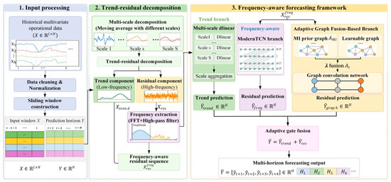
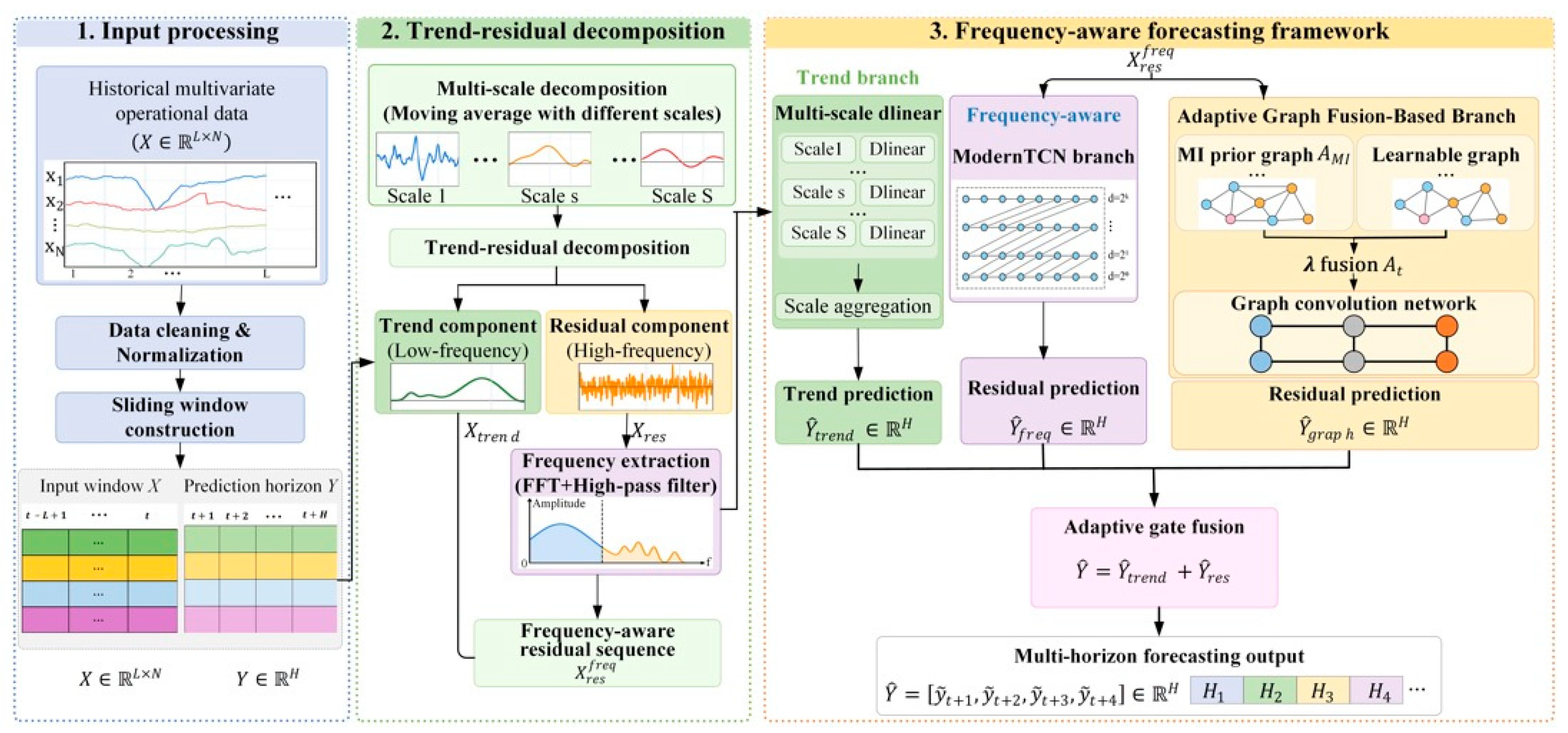
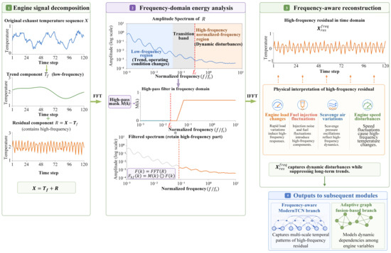
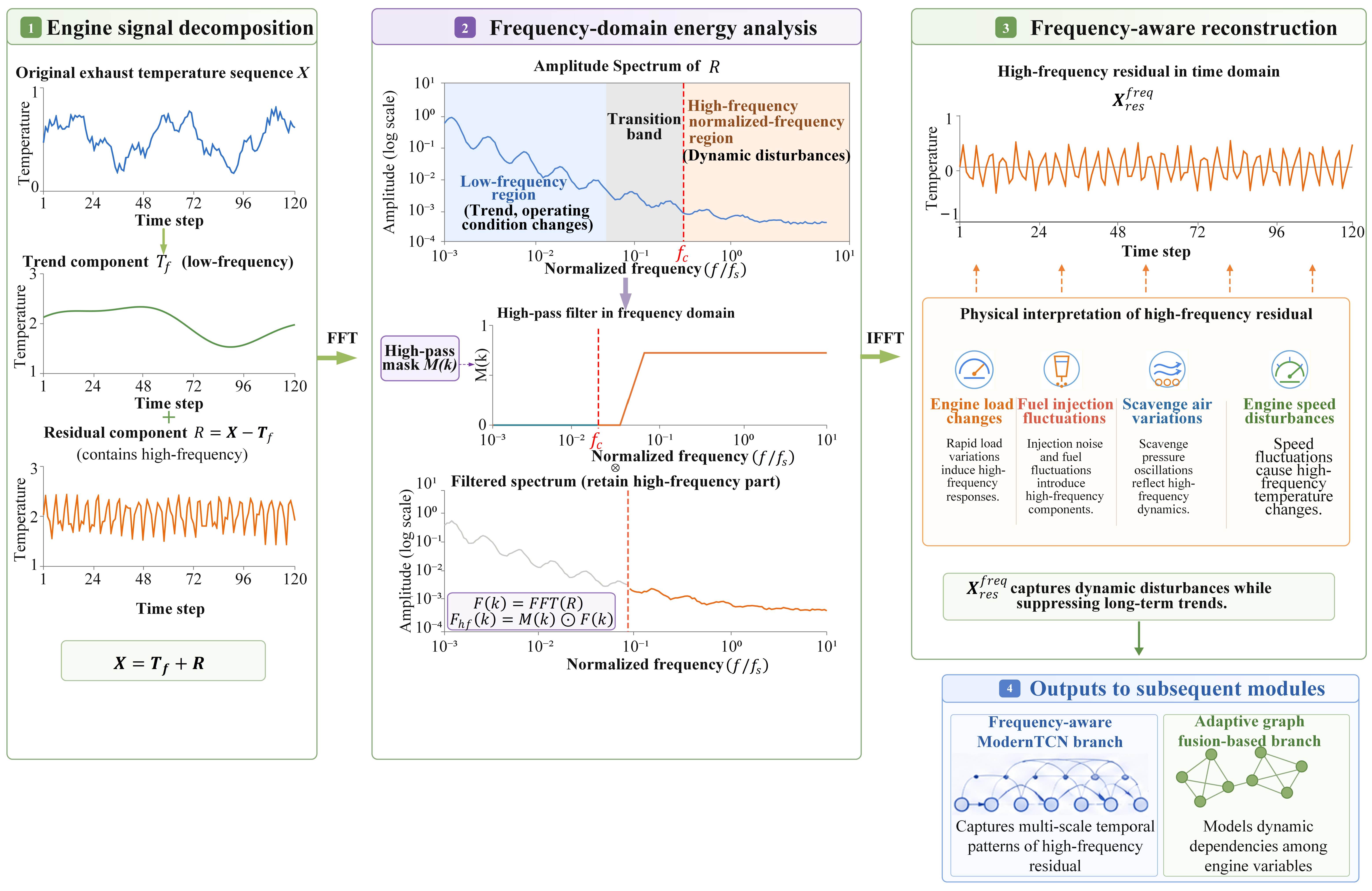
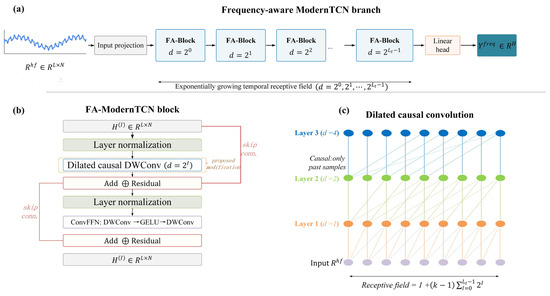
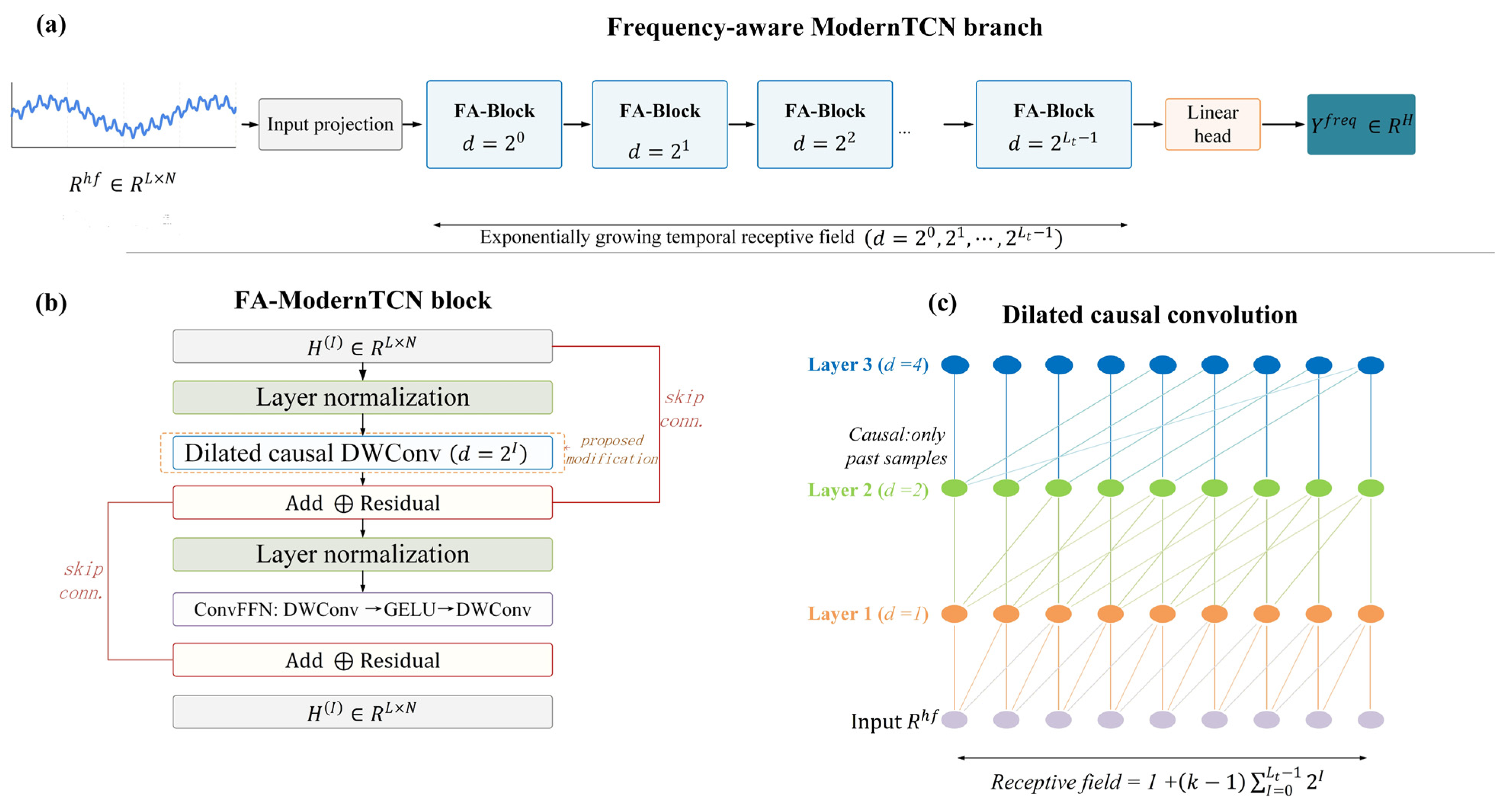
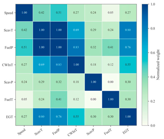
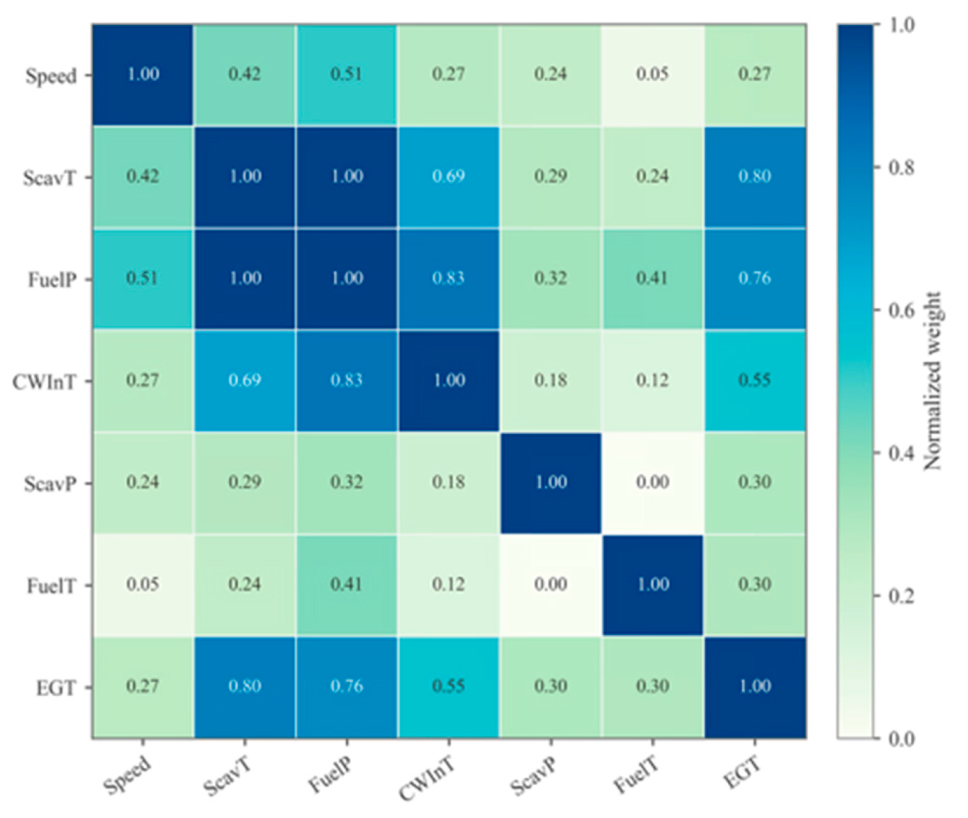
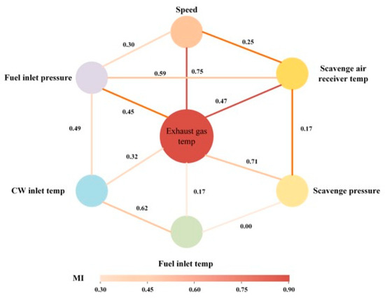
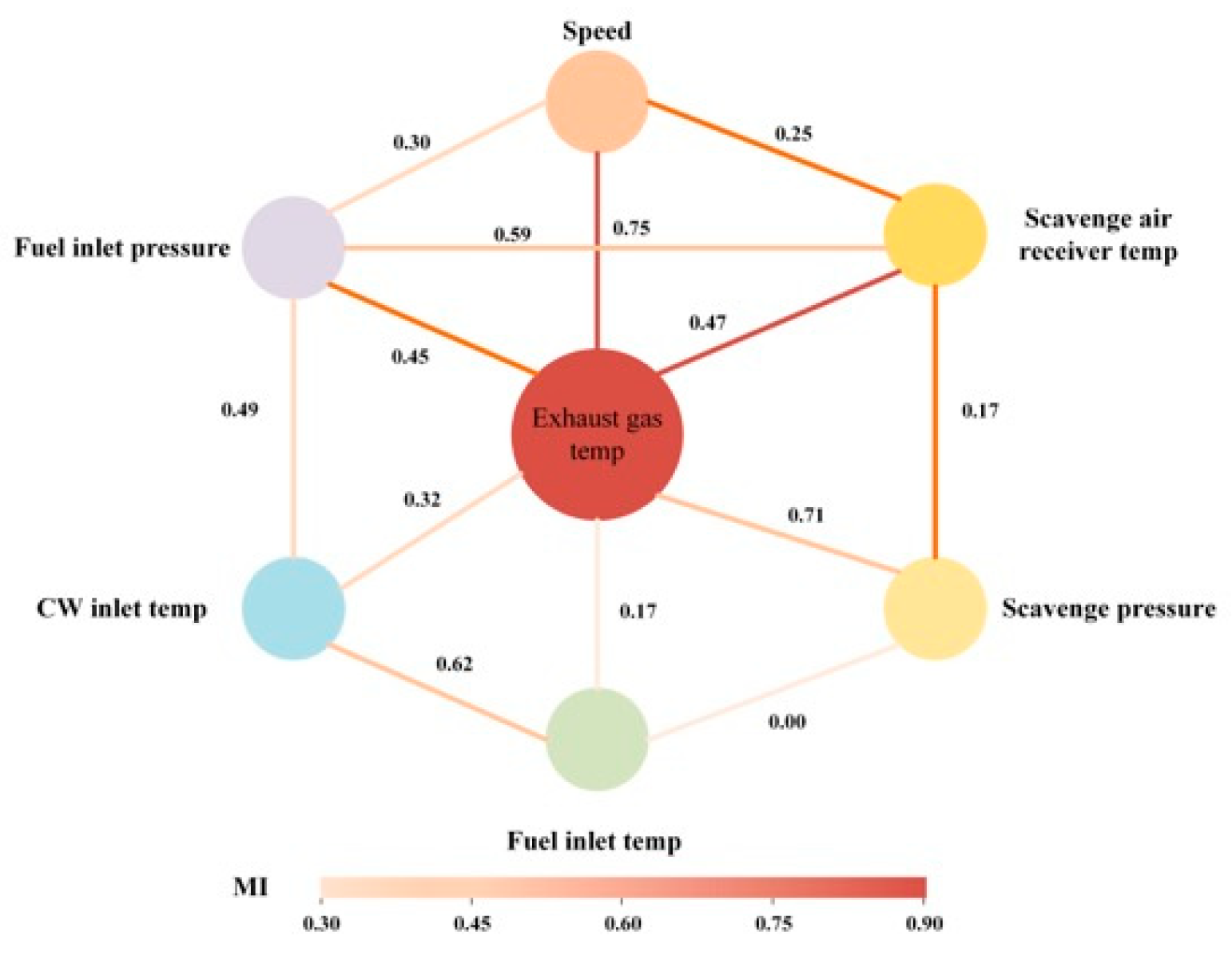
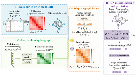
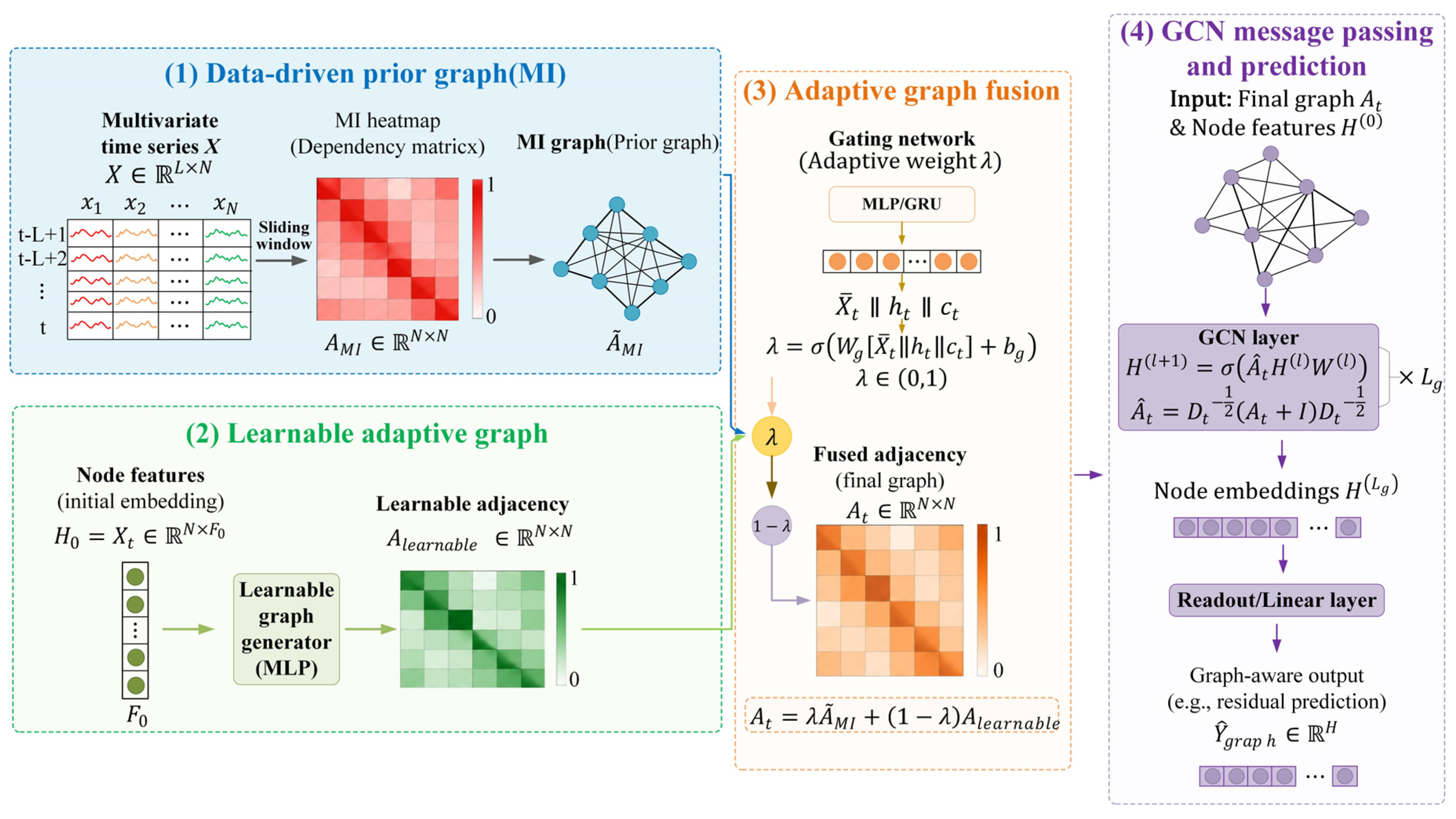
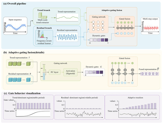
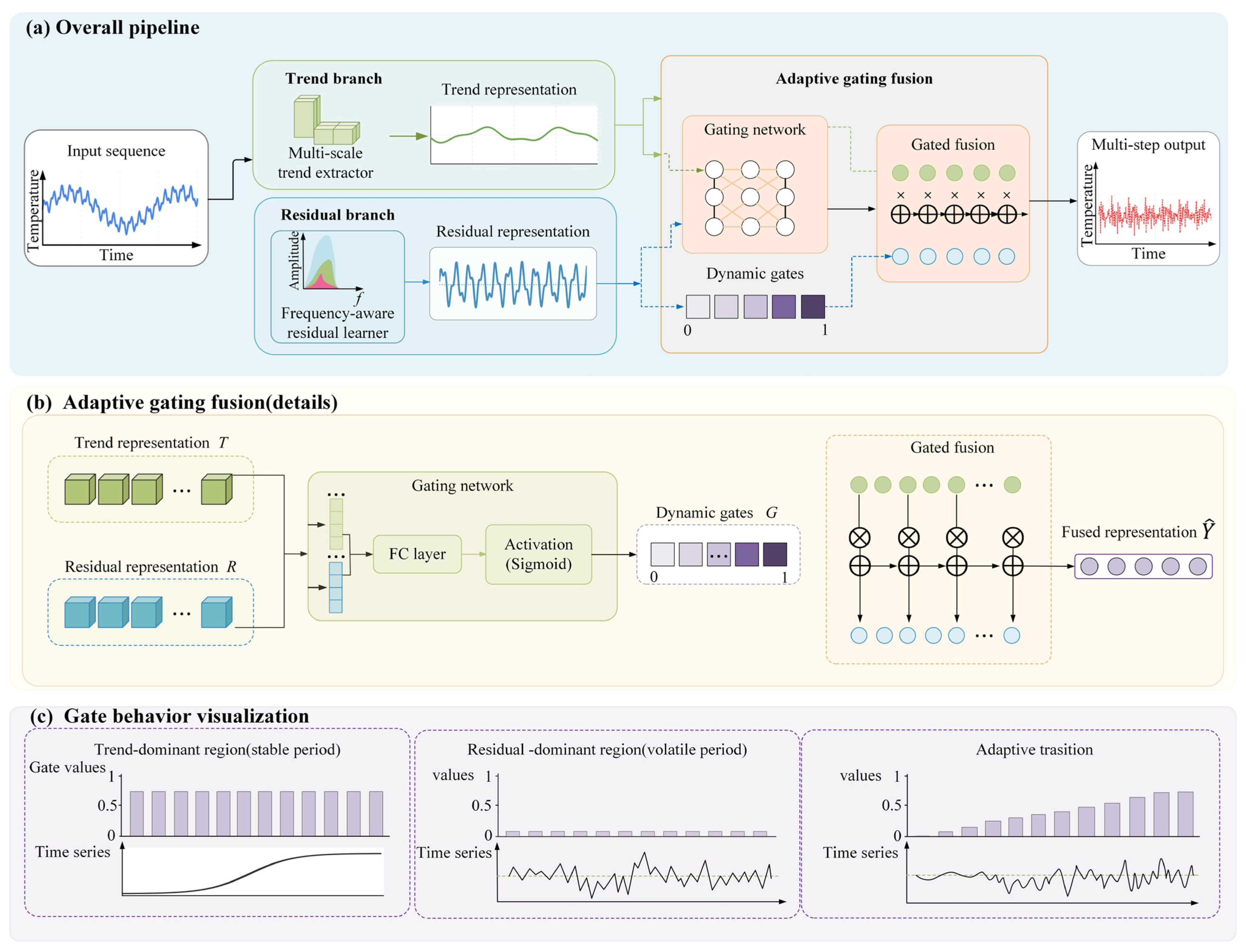
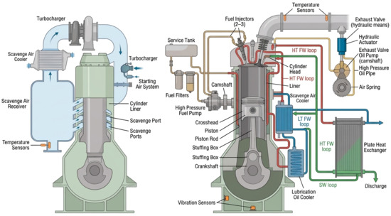
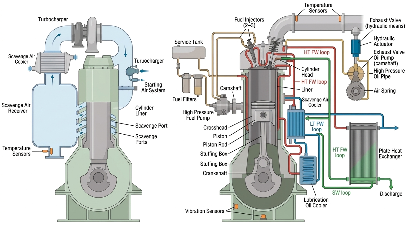
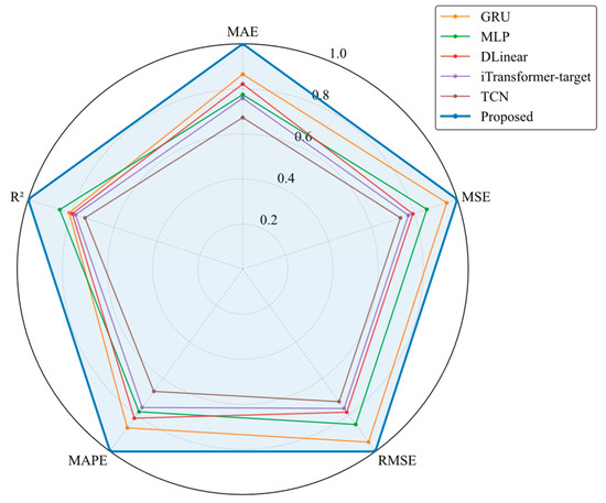
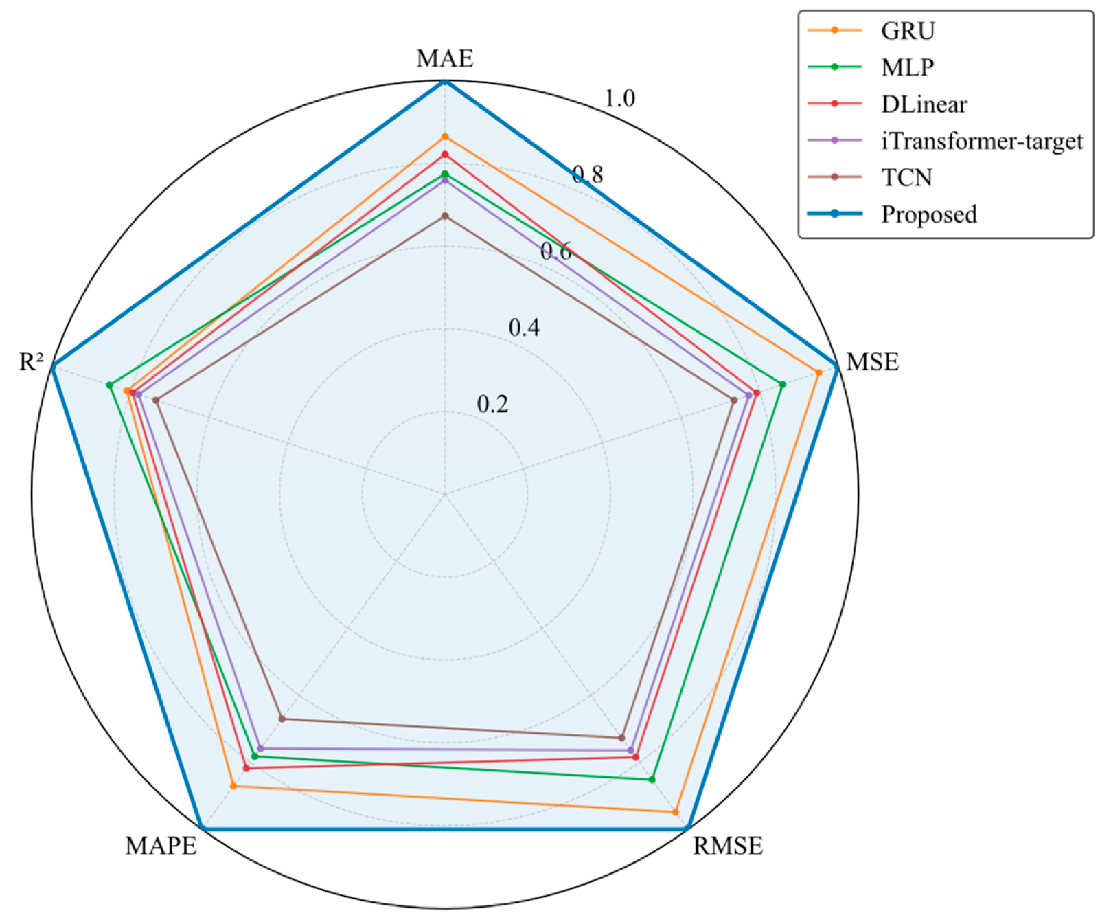
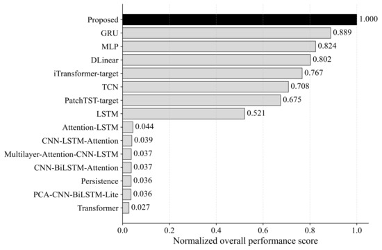
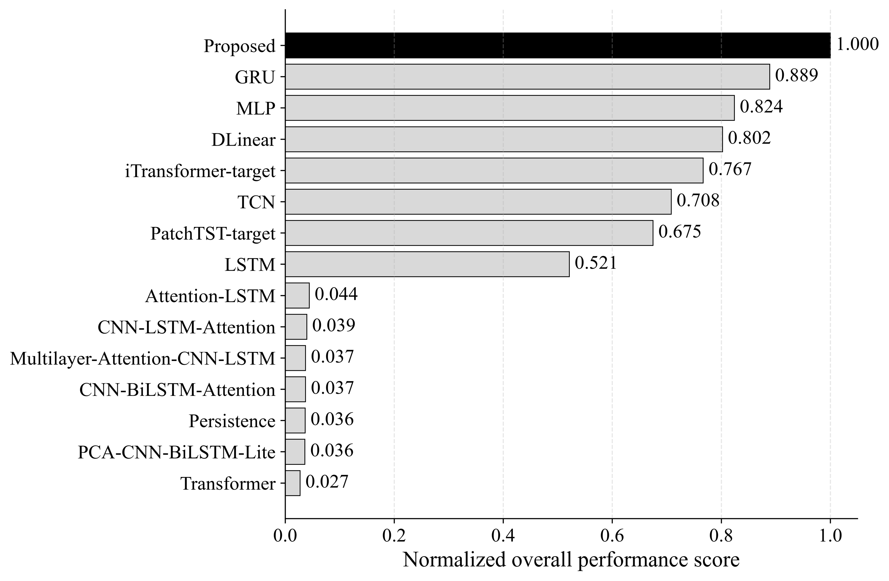
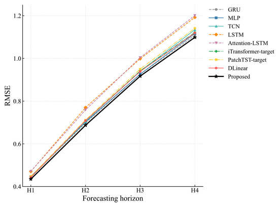
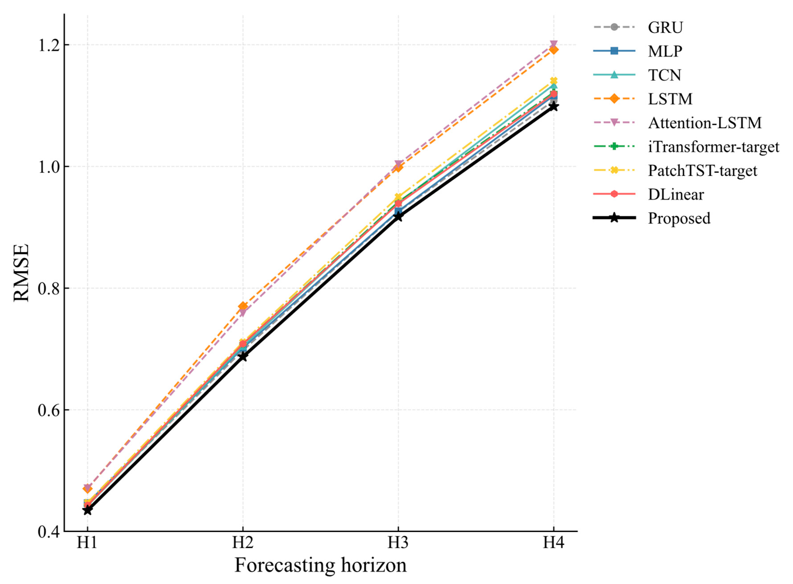
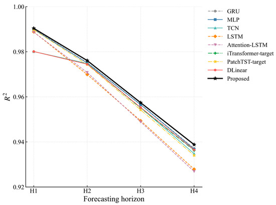
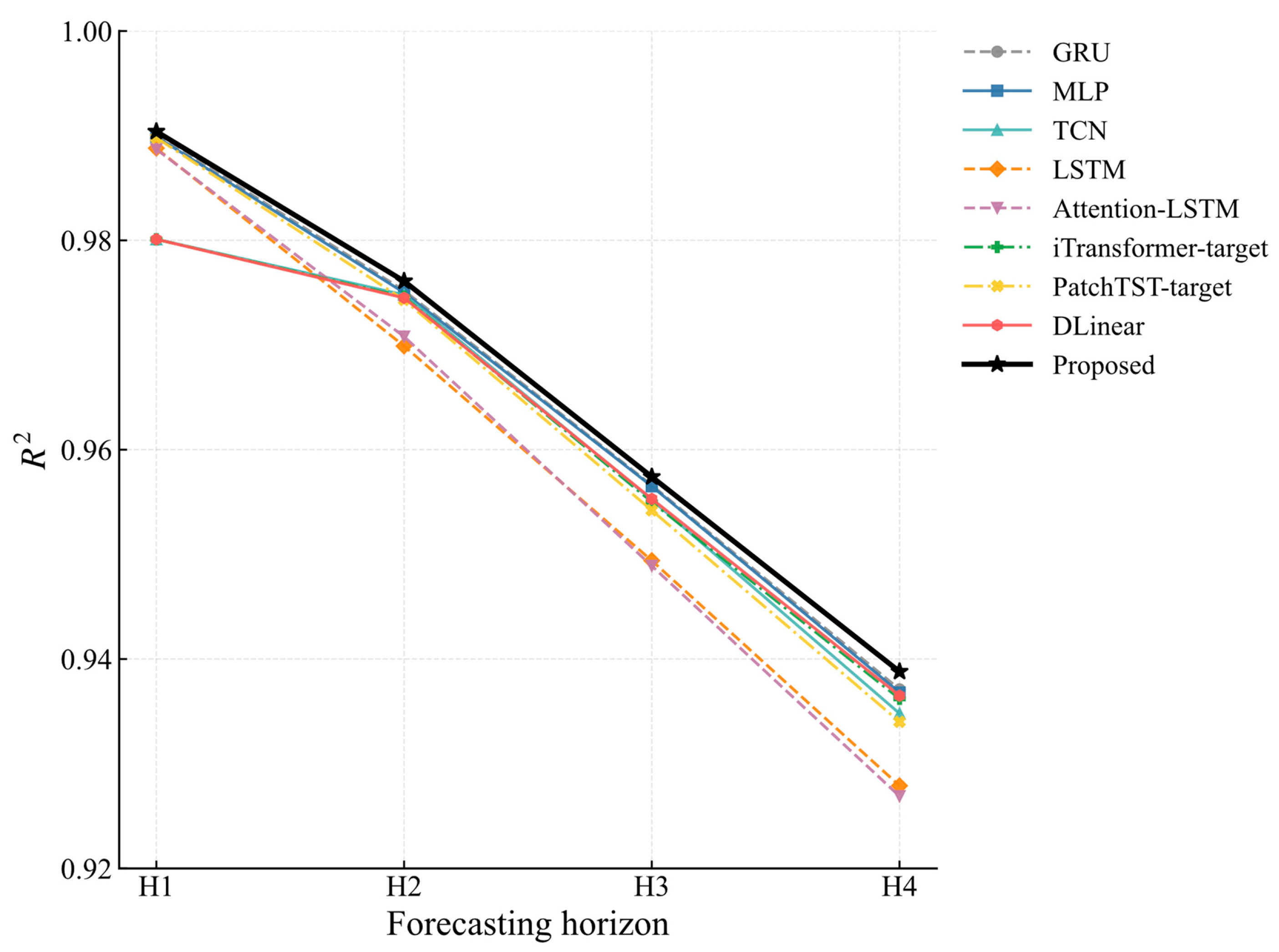
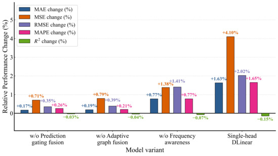
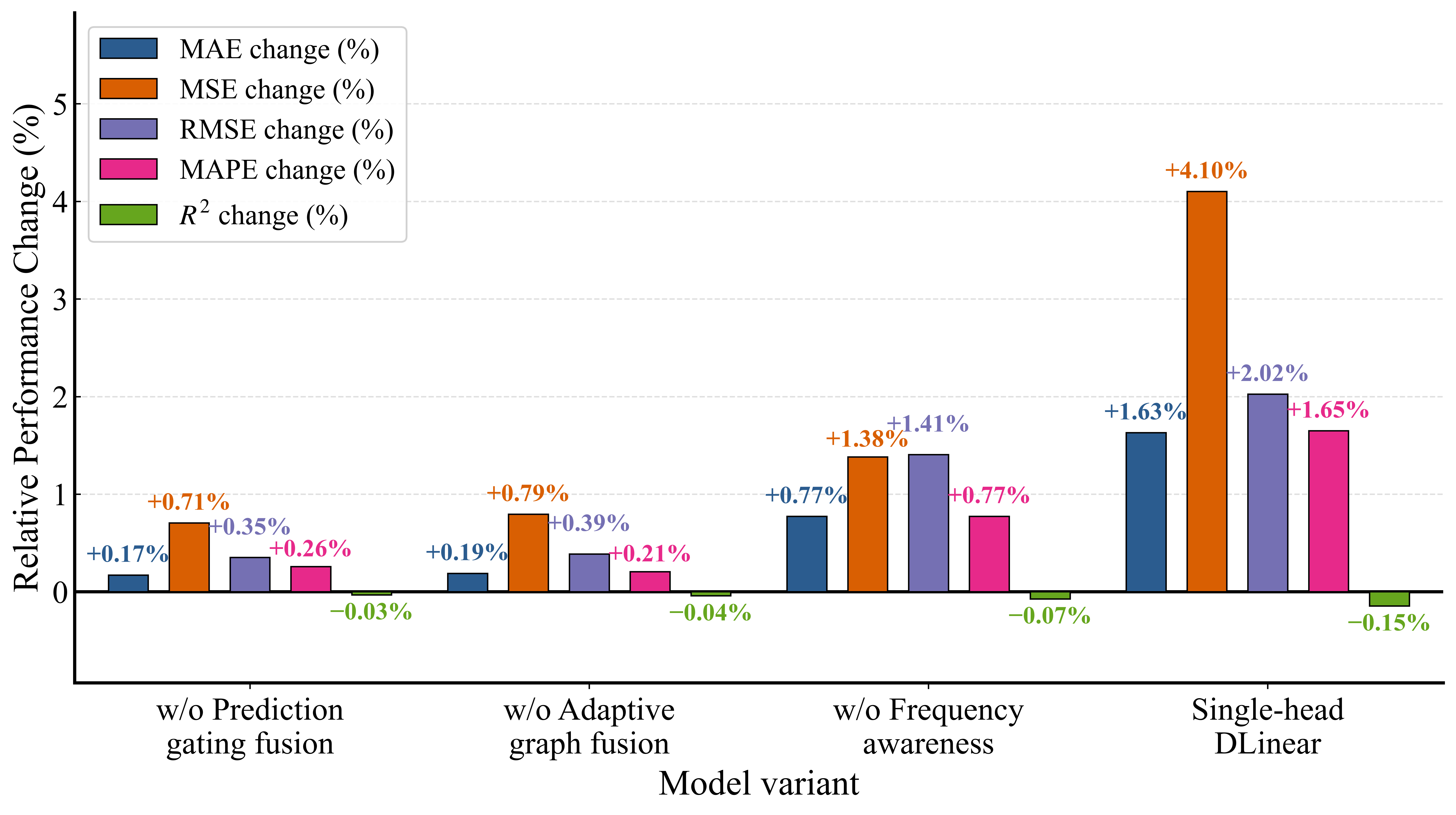
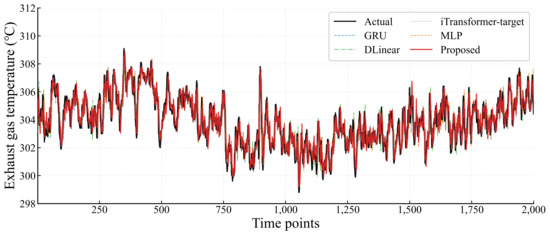
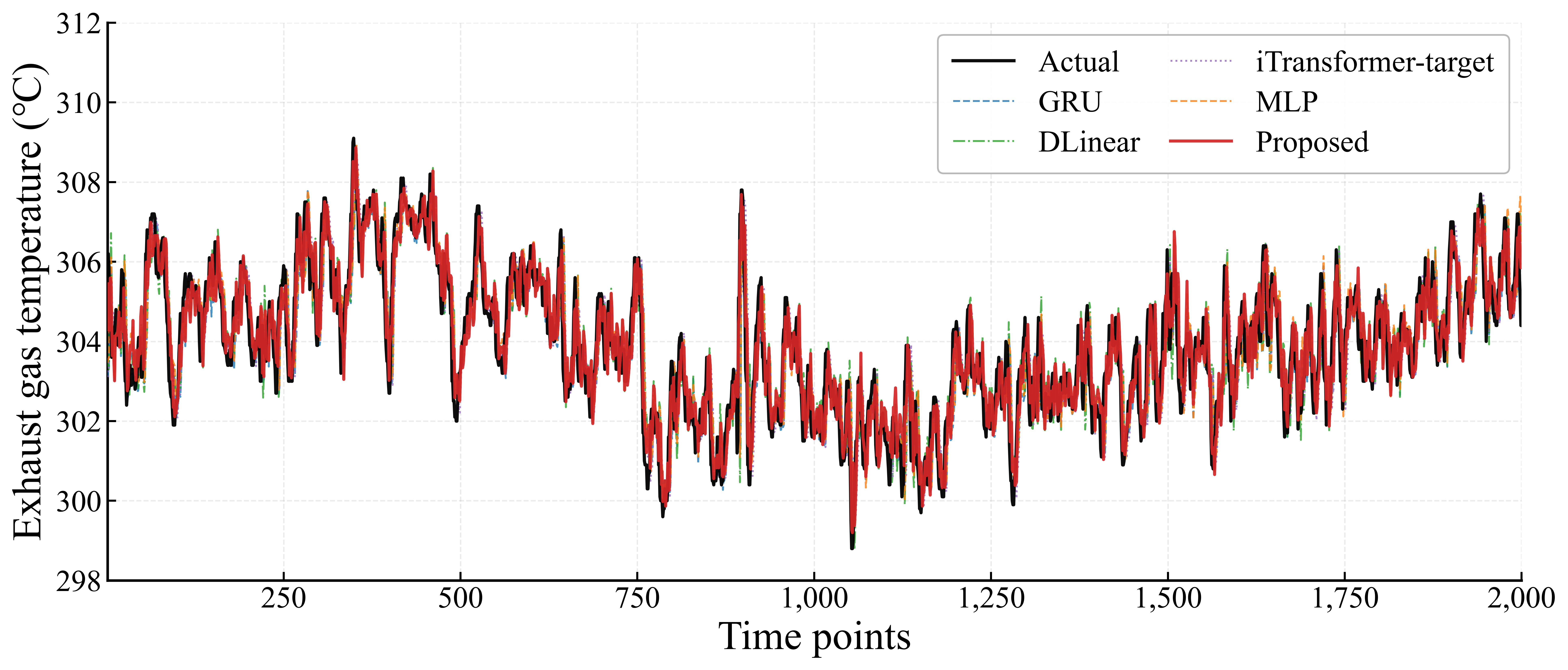
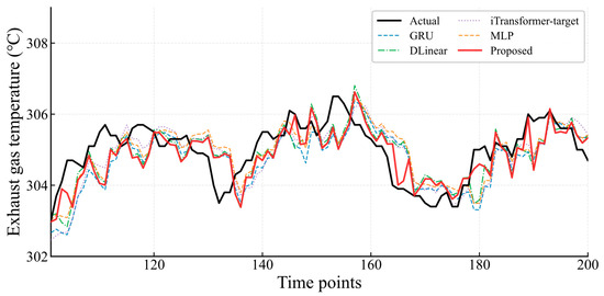
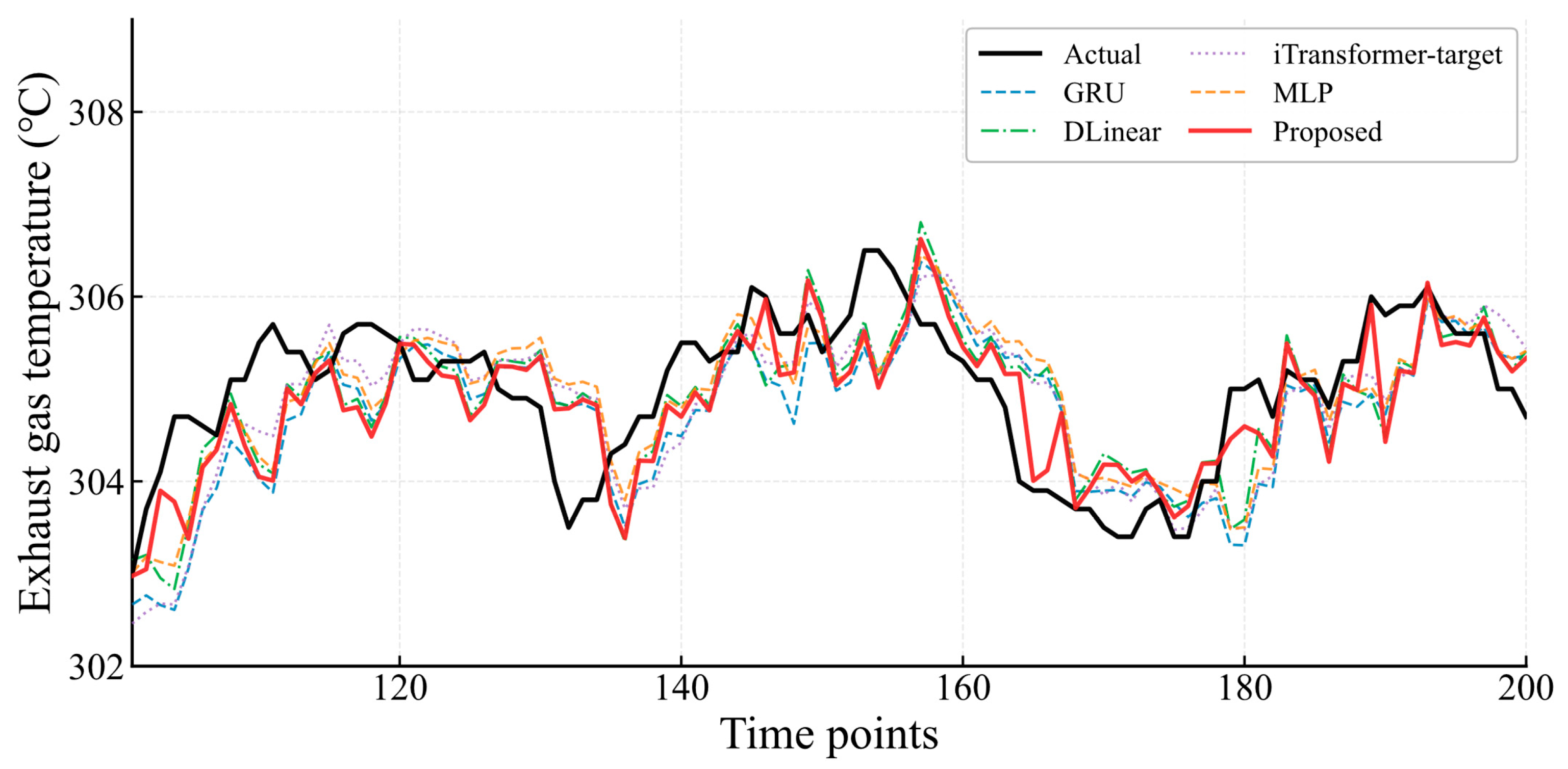
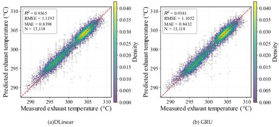
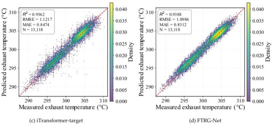
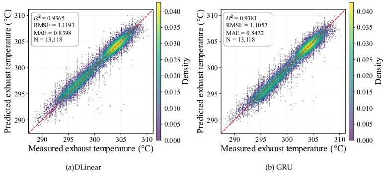
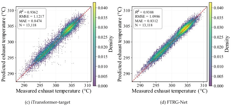
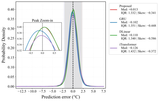
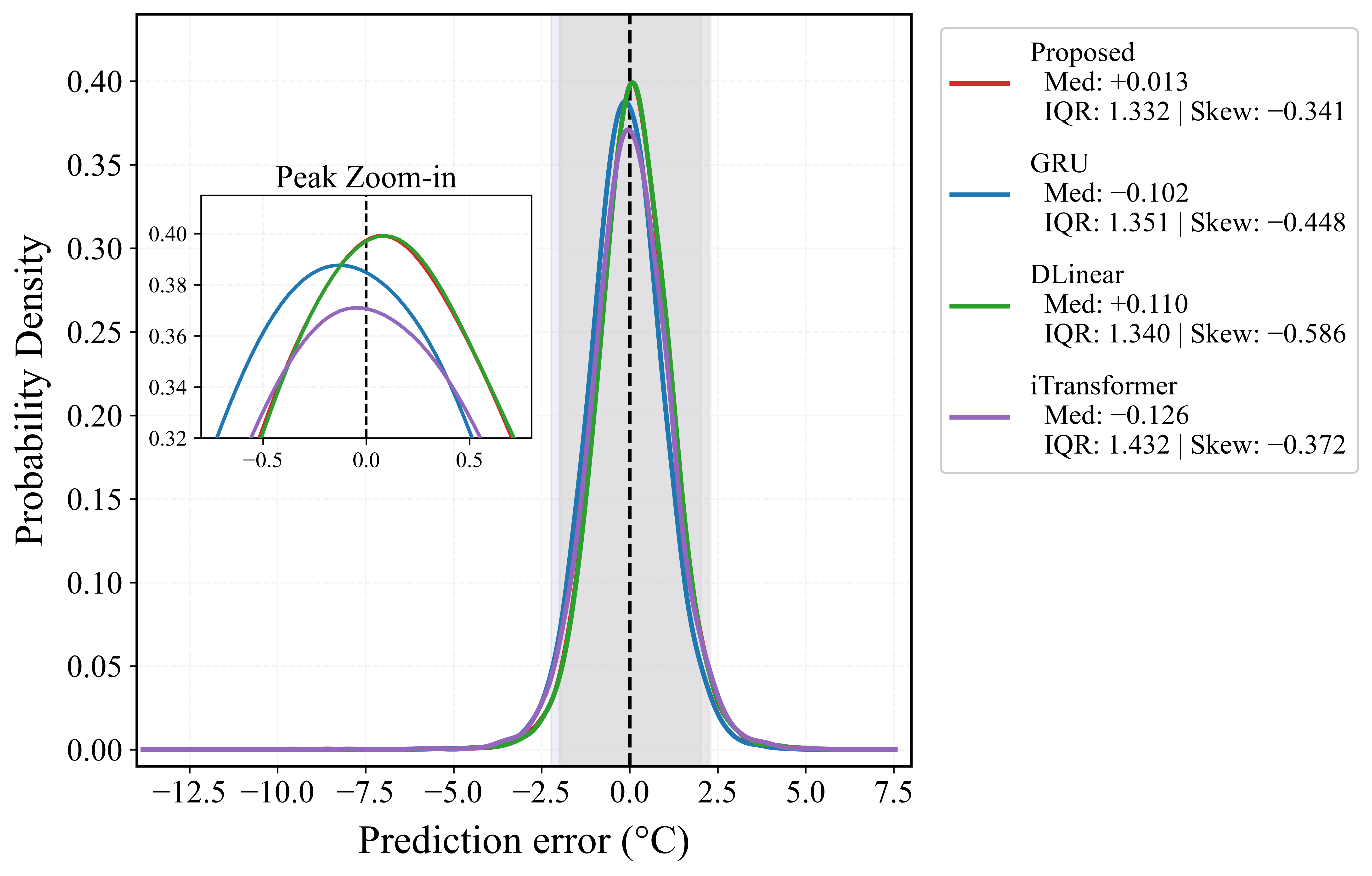
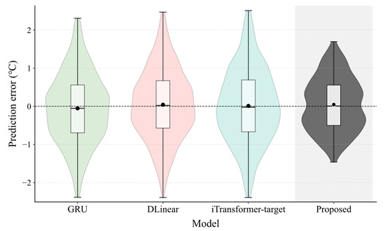
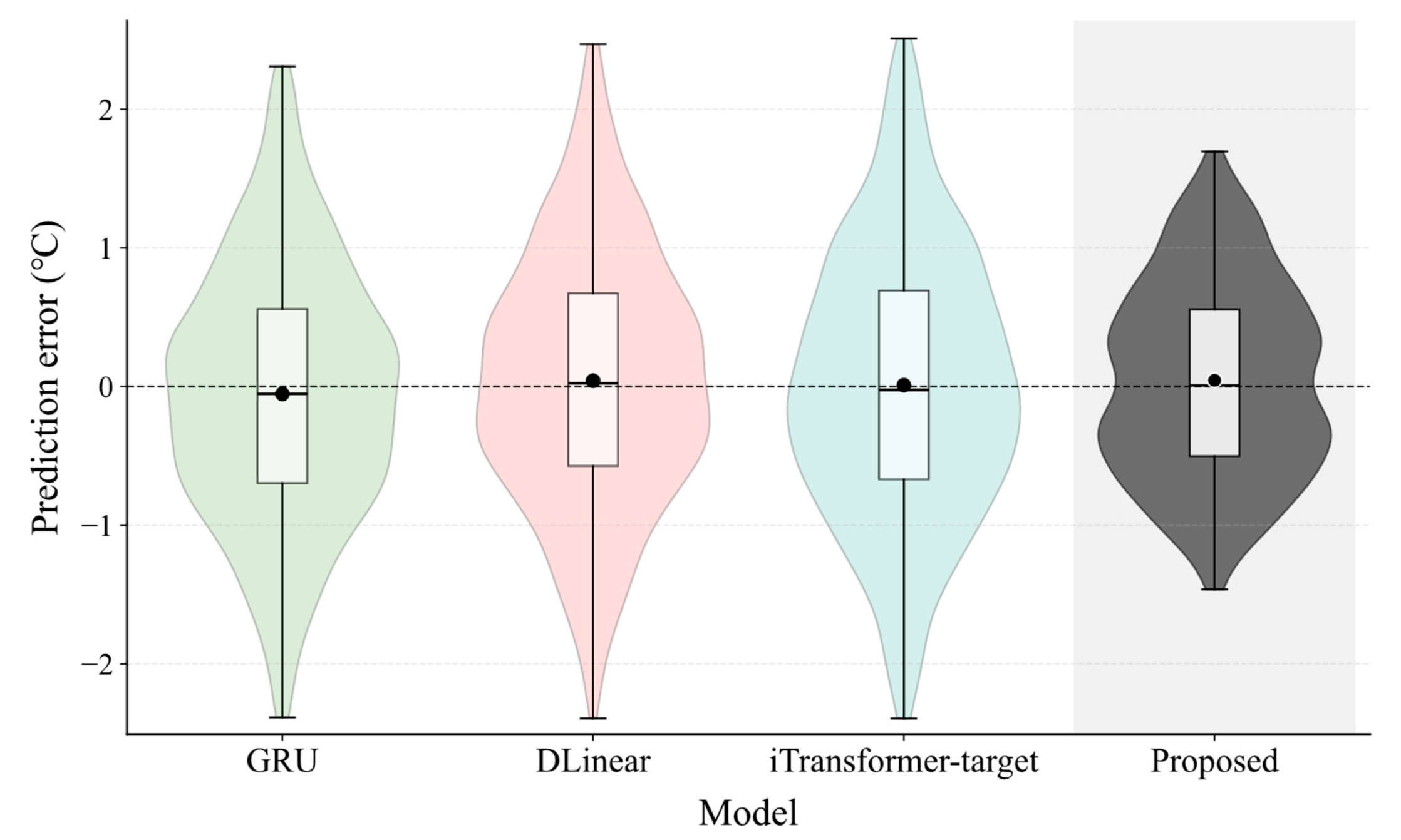
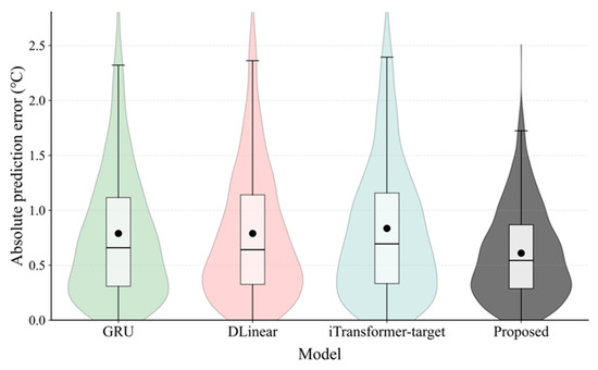
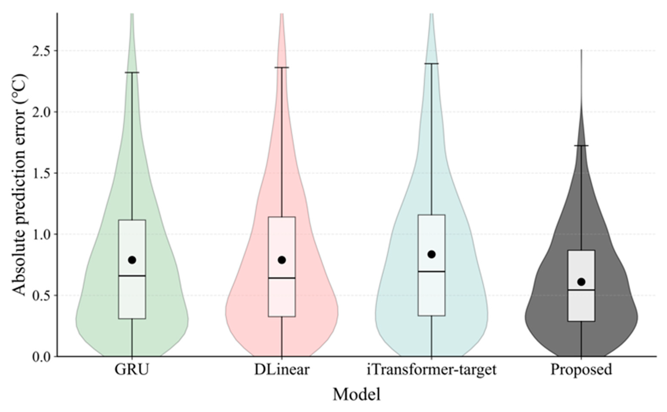
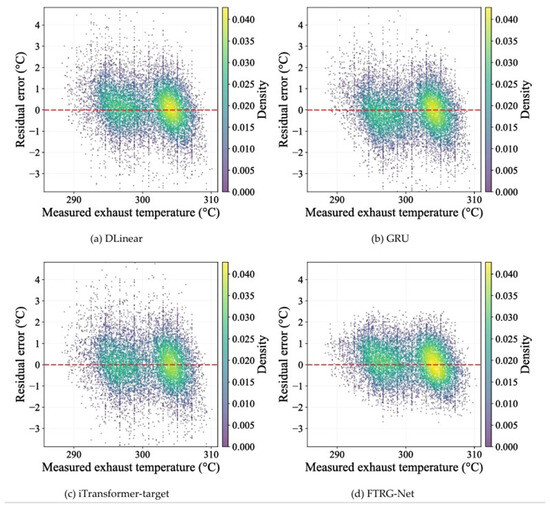
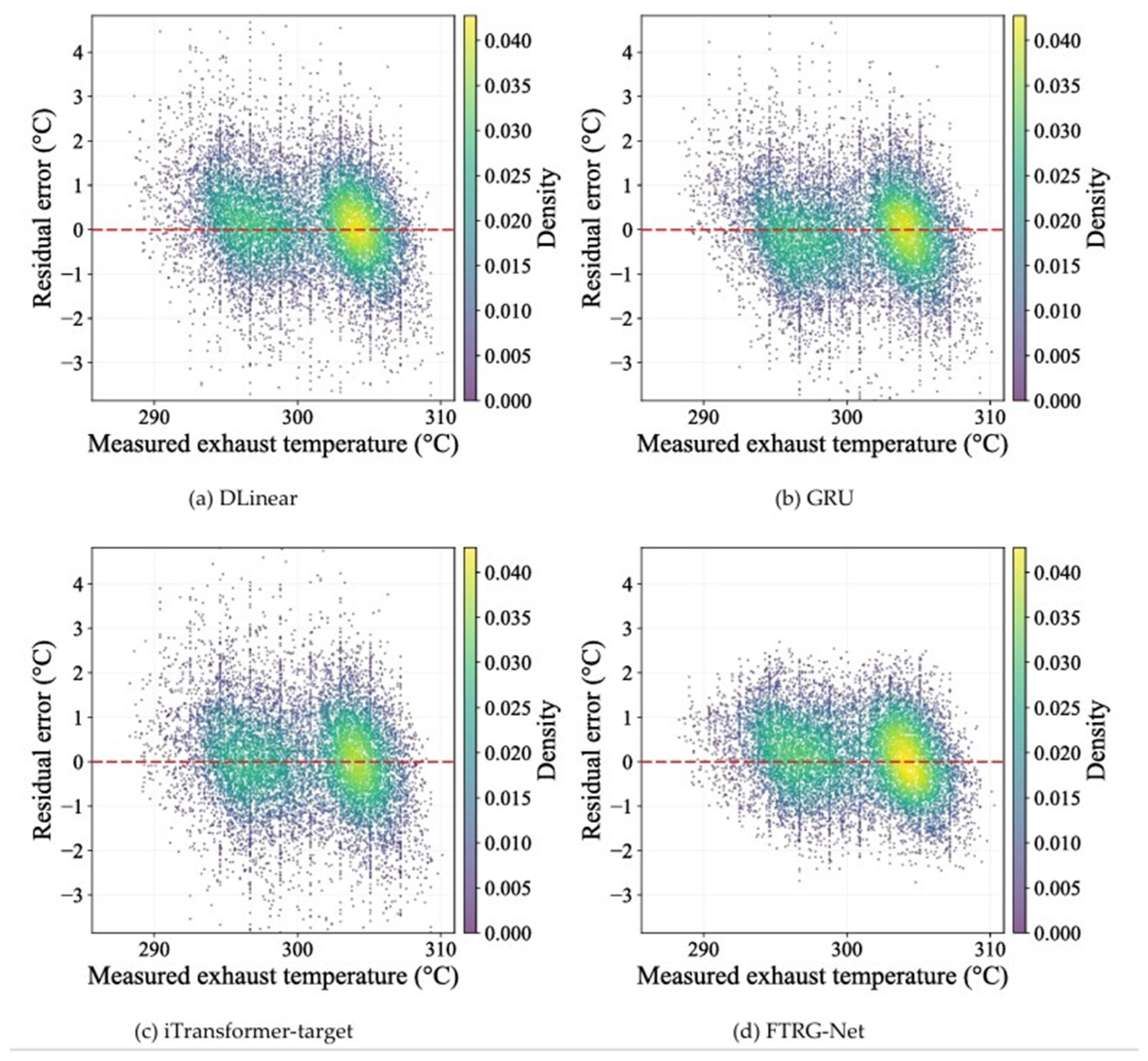

Disclaimer/Publisher’s Note: The statements, opinions and data contained in all publications are solely those of the individual author(s) and contributor(s) and not of MDPI and/or the editor(s). MDPI and/or the editor(s) disclaim responsibility for any injury to people or property resulting from any ideas, methods, instructions or products referred to in the content. |
© 2026 by the authors. Licensee MDPI, Basel, Switzerland. This article is an open access article distributed under the terms and conditions of the Creative Commons Attribution (CC BY) license.