Two As-Configured CFD Models (OpenFOAM and FLOW-3D) for Free-Surface Flow Through and Around Porous Coastal Structures

Abstract

Coastal defenses under tsunami-like long waves are judged not only by wave attenuation but by their own stability and the hazard left landward, so a porous structure is assessed through several responses at once. OpenFOAM (porousWaveFoam) and FLOW-3D HYDRO are the two models most widely used for such problems, representing the open-source and the commercial approach, and each has an extensive record for solitary waves and for porous structures separately. Which to adopt for a given response is not established, since the two have not been compared where both occur together. Five hydraulic benchmarks were, therefore, reproduced with both, taken as configured in practice, since the differing elements cannot be exchanged by the user. Agreement was decomposed into error components and into the scalars that enter a design check, and each difference was weighed against a combined uncertainty. Neither model is superior across the responses. Across 57 signals, the more accurate one changes with the metric in 81% of cases, and six of thirteen governing comparisons exceed the uncertainty. Some of the largest errors are shared, so changing the model does not remove them, and the cost ordering reverses with the problem size. Model selection should, therefore, follow the target design response, together with a statement of whether the difference exceeds the uncertainty. These findings hold within the configurations tested; extension to random waves remains for future work.

1. Introduction

Wave interaction with coastal structures is modeled with tools that range from depth-integrated models to interface-capturing Navier–Stokes solvers [1,2] and meshless particle methods [3,4], and the choice among them follows from the response to be predicted [5]. Where that response is local, such as the pressure on a structure or the flow within a porous body, a volume-of-fluid solver is the usual choice. Two such solvers are used widely in coastal engineering, OpenFOAM and FLOW-3D, and they represent the open-source and commercial approaches, respectively [5]. OpenFOAM is a platform rather than a fixed solver, and dedicated libraries for wave generation, absorption and porous media have been built on it and released openly [6,7,8,9,10,11,12]. FLOW-3D is an integrated commercial code in which those elements are supplied together. Its volume-of-fluid scheme keeps the interface sharp without resolving the air phase, and its fractional area/volume representation embeds geometry in a structured Cartesian mesh, so that no body-fitted grid is needed [13,14,15].

Solitary waves have been studied extensively with both models. With OpenFOAM, the run-up of solitary-wave trains on a uniform beach has been reproduced in detail [16], and the overland flow of broken solitary waves has been validated against large-scale experiments [17]. Solitary-wave overtopping of impermeable and porous revetments has been examined through the wave-generation toolboxes released for the platform [1,10,12]. The review of Huang et al. [5] catalogues a still-wider body of wave–structure applications built on it. FLOW-3D has an equally long record of application to the same condition. It has been used for solitary-wave run-up around conical islands and on non-planar beaches [18,19] and validated across the standard tsunami benchmark problems [20], for which its Cartesian meshing allows large domains to be set up quickly.

Porous coastal structures have likewise been studied extensively with both models. Within OpenFOAM, volume-averaged closures for flow through rubble mounds were formulated and validated against wave-basin measurements [6,7]. The porous-media equations and their resistance coefficients were re-examined in a dedicated series of studies [8,9], and the resulting models were applied to tsunami attack on rubble-mound breakwaters [21]. Within FLOW-3D, the flow between armor blocks has been resolved by building the individual units as geometry rather than as a porous medium [22], and run-up, reflection and overtopping have been simulated for breakwaters covered with antifer units [23]. The fractional-volume representation makes that geometric approach practical on a structured mesh.

Direct comparisons between the two models have been reported for a low Reynolds number hydraulic jump [10], for a vertical-slot fishway [11] and, most recently, for three-dimensional landslide-generated waves validated against a physical wave tank [12]. All three studies find that the two models reproduce the measured responses satisfactorily, while differing in the numerical treatment of the free surface and geometry and in the degree of user control. Sabeti et al. [12] describe them as representatives of the two principal classes of modeling tool in use. No comparison of this kind has yet been reported for solitary-wave interaction with porous coastal structures, where the two phenomena occur together.

That combination deserves separate treatment, because coastal defenses under extreme long waves are assessed not only for wave attenuation but for their own stability and for the hazard they leave landward [24,25]. Among long-wave conditions, the solitary wave has been a standard test case since Synolakis [26] because it isolates shoaling, run-up and overtopping in repeatable form [27]. It is not a surrogate for a real tsunami [28], but a standardized condition for testing robustness. When such a wave meets a porous structure, the external free-surface flow becomes coupled to seepage, inertial and drag resistance and dissipation within the body, and that coupling is governed by coefficients that must be specified rather than computed [8,9].

The way model performance is reported must also reflect the fact that a porous coastal structure is judged not by one response but by several. Run-up and overtopping govern the landward hazard and are checked against admissible overtopping limits [29]. Pressure and the accompanying suction govern the stability of the structure and its armor [30]. Transmitted and reflected heights govern sheltering, and the flow within the pores governs internal dissipation and the stability of the granular material [8,9]. These are different limit states, and a designer is normally concerned with one at a time, so the practical question is whether the prediction of that particular response can be relied upon.

These responses are not determined by the same part of a numerical model. The porous closure parameterizes the flow inside the medium, and so acts on quantities governed by that internal flow. Run-up and overtopping depend in addition on how a thin interface is advected and resolved. Local quantities near the structure depend on how its geometry is represented on the grid. Whether those correspondences hold, and whether two configurations diverge differently from one response to another, can be established only by decomposing the validation result rather than condensing it.

Conventional reporting practice is not well suited to this. Agreement is usually condensed into a single aggregate score, which introduces a further difficulty when two models are compared. If the ranking flips between responses or between spatial zones, differences of opposite sign are averaged together and can offset one another. The statistic may then report the models as indistinguishable, not because they agree but because quantities of an opposite sign have been summed. Deciding whether a difference is real further requires it to be weighed against the uncertainty of the comparison, for which a single score leaves no place. A similar need is identified by Koosheh et al. [31], who note that characterizing an individual wave rather than mean overtopping remains a challenge for high-fidelity modelling.

One further constraint governs how the comparison can be posed, since the two models are constructed differently. In OpenFOAM, the porous closure and its coefficients, the turbulence closure and the wave theory are each selected by the user, and a body of published practice has accumulated around those selections. In FLOW-3D, the same elements are supplied as one integrated package, and the points at which a user can intervene are deliberately few. These elements cannot be exchanged between the two, so whoever adopts either model adopts its porous closure, interface scheme and geometry treatment together. The two can, therefore, be compared only as complete configurations.

This study, therefore, pursues three aims. The first is to reproduce five hydraulic benchmark experiments with both porousWaveFoam and FLOW-3D, spanning porous infiltration, three-dimensional wave propagation, wave-induced pressure, slope run-up flow and overtopping. The second is to evaluate agreement through complementary error components together with the single quantities that enter a design check, rather than one averaged ranking, and to report the measured correlation structure of that metric set rather than assuming it. The third is to examine whether the relative performance of the two models is universal or reverses with the physical regime, spatial zone and motion phase, and, where it reverses, whether the difference exceeds the uncertainty of the comparison.

A comparison posed in this way does not return a single ranking. For each design quantity, it returns either a ranking that survives the uncertainty budget, or a statement that the two models are interchangeable for that quantity. The comparison also identifies responses in which both models err in the same direction, so that changing the model achieves nothing. Finally, it reports a computational cost whose ordering reverses with problem size.

2. Numerical Models

2.1. OpenFOAM (porousWaveFoam)

The first model is OpenFOAM (v2206), an open-source finite-volume framework. Several libraries have been built on it to couple wave generation and absorption with two-phase flow, among them waves2Foam [32], olaFlow [33] and IHFOAM [34].

Adopted here was waves2Foam. It generates and absorbs waves through relaxation zones, in which the target wave field is blended with the computed field over prescribed regions of the domain. Among its solvers, porousWaveFoam was selected because the structures considered include porous layers such as rubble-mound foundations and armor. It represents free-surface flow together with the dissipation and internal resistance of those layers. All meshes in this study were generated with blockMesh as structured orthogonal hexahedral grids. The porous structures are represented by assigning porosity and resistance to cell zones rather than by removing cells, so no body-fitting or mesh-snapping step is involved, and the grid topology is the same in every benchmark.

2.1.1. Governing Equations and Porous Resistance Model

To simulate flow through porous media, porousWaveFoam employs Volume-Averaged Reynolds-Averaged Navier–Stokes (VARANS) equations. This formulation uses volume-averaged quantities, thereby avoiding the direct resolution of microscopic interstitial flow. Relative to the standard incompressible Navier–Stokes equations, the VARANS formulation explicitly incorporates macroscopic porous-medium properties such as porosity and flow resistance. The continuity and momentum equations used in this study are given in Equations (1) and (2), respectively.

The flow between the pores is not laminar under most conditions of practical interest, but in a volume-averaged framework, that motion is not resolved. The averaging absorbs the net effect of pore-scale momentum exchange into closure terms, which is what allows the equations to represent a porous body without computing the interstitial flow.

$$\nabla \cdot \overrightarrow{U}=0$$

(1)

$$\left(1+C_m\right){\displaystyle \frac{\partial }{\partial t}}{\displaystyle \frac{\rho \overrightarrow{U}}{n}}+{\displaystyle \frac{1}{n}}\nabla \cdot {\displaystyle \frac{\rho }{n}}\overrightarrow{U}\overrightarrow{U}=-\nabla p^{*}+g\cdot \left(\overrightarrow{x}-{\overrightarrow{x}}_r\right)\nabla \rho +{\displaystyle \frac{1}{n}}\nabla \cdot \mu \nabla \overrightarrow{U}-{\overrightarrow{F}}_p$$

(2)

Here, $U$ denotes the filter (Darcy) velocity in the porous region, which is related to the actual pore velocity ${\overrightarrow{U}}_p$ through Equation (3). The variables $\rho$ and $\mu$ represent the mixture of density and dynamic viscosity, respectively; $t$ denotes time; $g$ is the gravitational acceleration; and $x$ and ${\overrightarrow{x}}_r$ are the spatial position vector and the reference water level vector, respectively. The term $p^{*}$ denotes the pseudo-dynamic pressure, defined as the total pressure excluding the hydrostatic component. The viscosity appearing in the diffusive term of Equation (2) is the total viscosity. That is, the sum of the molecular viscosity and the turbulent viscosity supplied by whichever turbulence closure is adopted. When no closure is used, the term reduces to its molecular value.

In Equation (2), the porous-medium effects are represented through the added-mass coefficient $C_m$ and the porous-resistance force ${\overrightarrow{F}}_p$. The coefficient $C_m$ accounts for the inertial effects associated with fluid acceleration within the porous matrix and is defined as a function of porosity using the empirical coefficient ${\gamma }_p$, as shown in Equation (4). Following Liu et al. [35], a value of 0.34 was adopted for ${\gamma }_p$. The porous-resistance force ${\overrightarrow{F}}_p$ is represented using the extended Darcy–Forchheimer formulation, in which linear and nonlinear drag components are superposed, as given in Equation (5).

$$\overrightarrow{U}=n{\overrightarrow{U}}_p$$

(3)

$$C_m={\gamma }_p{\displaystyle \frac{1-n}{n}}$$

(4)

$${\overrightarrow{F}}_p=a\rho \overrightarrow{U}+b\rho \left|\overrightarrow{U}\right|\overrightarrow{U}$$

(5)

$$a=\alpha {\displaystyle \frac{{\left(1-n\right)}^2}{n^3}}{\displaystyle \frac{\nu }{D_{50}^2}}$$

(6)

$$b=\beta \left(1+{\displaystyle \frac{7.5}{KC}}\right){\displaystyle \frac{1-n}{n^3}}{\displaystyle \frac{1}{D_{50}}}$$

(7)

The resistance coefficients a and b were determined from the characteristic grain size and porosity of the medium using the empirical relationships proposed by Van Gent [36], as given in Equations (6) and (7). In these expressions, $D_{50}$ denotes the median grain diameter of the porous medium, and $KC$ is the Keulegan–Carpenter number. The Keulegan–Carpenter number enters only through the bracketed factor of Equation (7), which corrects the non-linear coefficient for oscillatory flow. The value of 10,000 used here is the toolbox default [37] and places that factor at 1.00075, so the correction alters the non-linear coefficient by less than 0.1%, and the closure is evaluated in its steady-flow limit. The linear term represents the resistance governed by viscosity, and the non-linear term is governed by inertia and pore-scale turbulence. These are the coefficients that must be specified rather than computed, and they are the only quantities in the porous closure left to the user. The dissipation inside the porous body is, therefore, represented within the momentum equation itself, without a separate turbulence transport equation (Section 2.1.3).

For two-phase water-air flow, the free surface was tracked using the Volume of Fluid (VOF) method. Within the porous region, the transport equation for the water volume fraction F was modified to account for porosity, as shown in Equation (8) [8].

$${\displaystyle \frac{\partial F}{\partial t}}+{\displaystyle \frac{1}{n}}\left(\nabla \cdot \overrightarrow{U}F+{\overrightarrow{U}}_r\left(1-F\right)F\right)=0$$

(8)

Here, F denotes the water volume fraction in each computational cell, with $F=1$ for a cell completely filled with water and $F=0$ for a cell occupied entirely by air. The term ${\overrightarrow{U}}_r$ in Equation (8) is the artificial interface-compression velocity introduced to reduce numerical diffusion and maintain a sharp phase boundary. The mixture density $\rho$ and dynamic viscosity $\mu$ were evaluated as $F$-weighted averages of the liquid and gas properties, as given in Equations (9) and (10). This modified VOF treatment was used to maintain interface sharpness and numerical stability within the porous-flow simulations.

$$\rho =F{\rho }_l+\left(1-F\right){\rho }_g$$

(9)

$$\mu =F{\mu }_l+\left(1-F\right){\mu }_g$$

(10)

2.1.2. Wave Generation and Absorption Techniques in the Numerical Wave Flume

To reproduce solitary-wave conditions in the numerical wave flume while reducing contamination by reflected waves, the spatial-relaxation method implemented in waves2Foam was used. In this approach, relaxation zones are placed near the inlet and outlet boundaries, and the target wave field is gradually blended with the computed flow field through a spatial weighting function $w_R$. The resulting blended variable $\varphi$ is defined from the target value ${\varphi }_{target}$ and the computed value ${\varphi }_{computed}$, as expressed in Equation (11).

$$\varphi =\left(1-w_R\right){\varphi }_{target}+w_R{\varphi }_{computed}$$

(11)

Here, $\varphi$ denotes the blended field variable, such as velocity or volume fraction. The weighting factor $w_R$ varies smoothly according to the local coordinate $\sigma \in \left[0, 1\right]$ defined within the relaxation zone. To avoid the numerical instability associated with abrupt spatial gradients, an exponential weighting function was adopted, as given in Equation (12).

$$w_R=1-{\displaystyle \frac{\mathrm{e}\mathrm{x}\mathrm{p}\left({\sigma }^p\right)-1}{\mathrm{e}\mathrm{x}\mathrm{p}\left(1\right)-1}}$$

(12)

In Equation (12), p is the exponent controlling the shape of the weighting function; a value of p = 3.5 was adopted following the technical recommendations of the waves2Foam manual [38]. A relaxation zone was applied at the inlet only. There, the target solution was prescribed from the analytical wave theory corresponding to the imposed simulation condition, so that the computed field gradually developed into the intended incident wave. No relaxation zone was defined at the outlet. Outgoing flow leaves the domain through the downstream boundary, and no separate absorption layer was applied. FLOW-3D was likewise run without a sponge layer (Section 2.2.2), so that the outlet treatment is one of the elements matched between the two configurations.

2.1.3. Turbulence Treatment

The porousWaveFoam configuration was run without a turbulence closure, so that the effective viscosity in the momentum equation reduces to its molecular value. Since the FLOW-3D configuration uses a $k-\epsilon$ closure, this is a user choice and appears in group C of

Table 1. Classification of the elements of the comparison.

Group	Element	porousWaveFoam	FLOW-3D HYDRO, Solver Build 25.1.0 (Double Precision)
A. Matched	Geometry, water depth, wave height, simulated duration	Identical	Identical
	Porous medium: D50 and porosity n	Identical	Identical
	Total cell count	Matched to within a few percent (Experiments 2–5)	Matched to within a few percent (Experiments 2–5)
	Cell topology	Orthogonal hexahedra (blockMesh); no body-fitting	Orthogonal Cartesian cells; geometry by FAVOR
	Outlet treatment	No absorption layer	No absorption layer
	Resistance-coefficient tuning	None performed	Not applicable
B. Not exchangeable	Porous closure	van Gent form; α and β taken from the literature	Built-in grain-diameter drag model; no equivalent coefficients exposed
	Solitary-wave theory at generation	Chappelear [39], imposed through a relaxation zone	McCowan [40], imposed directly at the boundary
	Free-surface algorithm	Algebraic VOF with interface compression	TruVOF
	Geometry representation	Structure represented by assigning porosity and resistance to a cell zone; cells are not removed, so the boundary follows cell faces	Geometry embedded by FAVOR through the fractional open area and volume of each cell, so a cell may be partially open
	Air phase	Resolved (two-phase)	Not resolved (one-fluid free-surface mode)
	Pressure–velocity coupling	PIMPLE in PISO mode; PCG–DIC	GMRES
C. Not matched by choice	Turbulence closure	None (laminar); see Section 2.1.3	k–ε
	Momentum advection	Second order (limitedLinearV)	First order
	Computing hardware	6-core Intel Core i7-8700	64-core AMD Ryzen Threadripper PRO

. Turbulence inside the porous body is not thereby disregarded. As set out in Section 2.1.1, the effect of pore-scale turbulence is carried by the non-linear term of the Darcy–Forchheimer closure at every time step. What the choice determines is the treatment outside the porous body, in the free-surface region and in the shear layers near the structure.

Three considerations govern it. The waves2Foam formulation applies volume-averaging corrections to the momentum and volume-fraction equations but not to the turbulence transport equations, and none of the standard OpenFOAM closures carries the porosity scaling that consistency would require [38]. Activating one inside the porous region would superimpose an eddy-viscosity dissipation on the Forchheimer term, counting the same dissipation twice. Standard two-equation closures are also reported to over-produce turbulence near the free surface and to damp propagating waves [5]. The relaxation zone corrects the velocity and volume-fraction fields but not the turbulence quantities, so that turbulence would be advected along the flume before reaching the structure. The established porousWaveFoam validation studies for this class of problem adopt the same configuration [8,35]. The limitation is that turbulence outside the porous body, in breaking, in shear layers, and in aerated run-up, is not resolved. Where that matters for a particular response, it is identified in Section 3.

2.2. FLOW-3D

The second model is FLOW-3D HYDRO (Flow Science, Inc., Santa Fe, NM, USA; solver build 25.1.0), a commercial finite-volume code, referred to below as FLOW-3D. FLOW-3D tracks the free surface using the TruVOF method and represents complex solid geometry on a Cartesian grid using the Fractional Area Volume Obstacle Representation (FAVOR) method [15]. In the present study, the built-in porous-media model was used to represent porosity and internal flow resistance within porous layers such as the rubble-mound foundation and armor units. Turbulence outside the porous body was carried by the k–ε closure supplied with the code (

Table 2. Numerical settings of the two configurations in the detail needed to reproduce the simulations.

Item	porousWaveFoam	FLOW-3D
Version	OpenFOAM v2206 with waves2Foam	FLOW-3D HYDRO, solver build 25.1.0 (double precision)
Time integration	Euler, first-order implicit	Automatic time-step control
Momentum advection	Gauss limitedLinearV	First order
Volume-fraction advection	Gauss vanLeer with interface compression	TruVOF, automatic scheme selection
Interface compression	cα = 1; MULES corrector off	Not user-specified
Gradient and Laplacian	Gauss linear; Gauss linear corrected	Not user-specified
Pressure–velocity coupling	PIMPLE, one outer and three inner correctors	GMRES
Linear-solver tolerances	10−8 (α); 10−7 (p_rgh); 10−6 (U)	Solver default
Time-step control	Adjustable; Courant number 0.5, interface Courant number 0.25; initial Δt = 0.005 s, maximum Δt = 0.01 s	Automatic stability limit
Turbulence closure	None (laminar)	k–ε
Air phase	Two-phase; air resolved	One-fluid; air not resolved
Convergence criterion	Fixed tolerances, as above	Automatic
Wall treatment	No-slip; no wall function (laminar)	No-slip; roughness height 0 m
Mesh generation and quality	Structured orthogonal hexahedral grid generated with blockMesh; porous regions defined as cell zones within the same grid. Maximum non-orthogonality 0° and maximum skewness 0 by construction; no mesh-motion or body-fitting step. The grid is uniform, so the resolution at the free surface equals the cell size everywhere; no local refinement was applied	Structured Cartesian grid; geometry embedded through FAVOR. Cells orthogonal by construction
Porous drag model	van Gent formulation, Equations (5)–(7)	Grain diameter calculated drag model
Porous–clear-fluid interface	Volume fraction transported with the porosity correction of Equation (8); no explicit interface condition imposed	Handled internally through the FAVOR open-volume and open-area fractions

).

2.2.1. Governing Equations

FLOW-3D solves the continuity and Navier–Stokes equations on a Cartesian grid. Within this framework, the FAVOR method represents complex geometry and porous obstruction through the open-volume fraction $V_F$ and the open-area fraction $A$ in each computational cell. The governing equations used in this study are given in Equations (13) and (14).

$$V_F{\displaystyle \frac{\partial \rho }{\partial t}}+\nabla ·\left(\rho UA\right)=0$$

(13)

$${\displaystyle \frac{\partial U}{\partial t}}+{\displaystyle \frac{1}{V_F}}\left(UA·\nabla \right)U=-{\displaystyle \frac{1}{\rho }}\nabla p+g+f_v-F_P$$

(14)

In these equations, $U$ denotes the velocity vector, $\rho$ is the fluid density, $P$ is the pressure, $g$ is the gravitational acceleration, and $f_v$ represents the viscous stress term. The term $F_P$ in Equation (14) denotes the flow resistance generated within the porous medium. In the present study, the built-in grain-diameter-based drag model of FLOW-3D was used to represent porous resistance. This model evaluates laminar and turbulent resistance from the porosity $n$ and the representative grain diameter $D_{50}$ of the porous structure. To maintain consistency between the two numerical models, the same $D_{50}$ and porosity values were applied in both porousWaveFoam and FLOW-3D.

$${\displaystyle \frac{\partial F}{\partial t}}+{\displaystyle \frac{1}{V_F}}\nabla ·\left(FUA\right)=0$$

(15)

The free surface was tracked using the TruVOF method. The transport equation for the fluid volume fraction $F$ includes the FAVOR terms, as shown in Equation (15), so that volume conservation can be maintained within the porous region. Here, $F=1$ denotes a cell completely filled with fluid, whereas $F=0$ denotes a cell without fluid.

2.2.2. Wave Generation and Absorption Techniques

To generate solitary waves in FLOW-3D, the built-in wave-generation boundary condition was applied at the inlet, with the water-surface profile and velocity distribution prescribed from the McCowan solitary-wave theory [40] implemented in FLOW-3D.

At the inflow boundary, the water level and velocity were imposed directly over time to generate the target solitary wave. FLOW-3D provides a sponge-layer-type absorption capability, but it was not used in the present simulations. The downstream boundary was set as an outflow boundary so that transmitted flow leaves the domain directly, matching the porousWaveFoam outlet treatment described in Section 2.1.2.

2.3. Elements of the Comparison

The two models differ in mesh generation, free-surface treatment, geometry representation and porous-media implementation. Since such differences may affect how each reproduces a given response, Table 1 sorts them into three groups before any result is presented. Group A holds elements that were made identical in the two models, group B those that the released codes do not allow a user to make identical, and group C those that could have been made identical but were not.

Group B matters most. Its items cannot be exchanged by a user. The free-surface algorithm of one code cannot be run inside the other. The fractional cell occupancy of FAVOR has no counterpart in the cell-zone assignment used by porousWaveFoam, and the porous model of FLOW-3D gives the user no coefficients corresponding to $\alpha$ and $\beta$. Anyone comparing the two models as they are actually used, therefore, carries these differences with them, and they are treated here as part of what is being compared. What follows is thus a response-dependent validation of two configured models, rather than a ranking of two software packages. Group C holds the turbulence treatment (Section 2.1.3), the order of the momentum advection scheme, which both codes let the user set but which was left as adopted in each, and the computing hardware (Section 3.3). Because the group B differences act at the same time, a discrepancy is not ascribed to one of them unless a separate test can isolate it. Where a mechanism is suggested by the components, it is identified as a candidate rather than as a cause. The numerical settings of the two configurations are listed in Table 2 in the detail required for the simulations to be reproduced.

3. Validation Metrics and Model Validation

This section defines the measures used to compare the two models with the reference experiments and reports the results for the five benchmarks. It then examines the computational cost, the accuracy–cost relationship, and the conditions under which a difference between the two is large enough to act upon.

3.1. Validation Metrics

For the reasons set out in Section 1, agreement is not condensed here into a single score. The measures used instead follow the error-variance decomposition of Murphy [41], in which the mean-square error separates into bias, amplitude and correlation contributions, each isolating one way in which a signal can depart from the measurement.

Table 3. Decomposed validation metrics used in this study.

Group	Indicator	Definition	Meaning
A. Error components	Normalized bias,  b	${\displaystyle \frac{\overline{R_{model}-R_{obs}}}{R_{ref}}}$	Systematic over/under-prediction
	Amplitude ratio, ${\sigma }^{*}$	${\displaystyle \frac{{\sigma }_{model}}{{\sigma }_{obs}}}$	Whether response magnitude is reproduced
	Correlation, $R$	$corr\left(R_{model},R_{obs}\right)$ at zero lag	In-place temporal agreement
	Shape correlation, $R_{shape}$	${max}_s corr\left(R_{model}\left(t+s\right),R_{obs}\right)$	Waveform similarity (≥$R$)
	Phase lag, ${\tau }^{*}$	$[arg ma{x}_s corr]\times \Delta t$	Timing error of the primary event
	Waveform-duration ratio, $T_w^{*}$	${\displaystyle \frac{T_{w,model}}{T_{w,obs}}}$, $T_w=\surd \left({\displaystyle \frac{\int {\left(t-\overline{t}\right)}^2{R}^{+}dt}{\int R^{+}dt}}\right)$	Whether the event is too short/long
B. Design scalars	Peak error, ${\Delta }_{peak}$	${\displaystyle \frac{R_{model,peak}-R_{obs,peak}}{R_{ref}}}$	Peak response intensity
	Positive impulse error	${\displaystyle \frac{\int {R^{+}}_{model}dt-\int {R^{+}}_{obs}dt}{\int {R^{+}}_{obs}dt}}$	Cumulative load-related intensity
	Suction impulse error	${\displaystyle \frac{\int {R^{-}}_{model}dt-\int {R^{-}}_{obs}dt}{\int {R^{-}}_{obs}dt}}$	Cumulative suction on the structure
C. Overall summaries	$NRMSE$	${\displaystyle \frac{RMSE\left(R_{model},R_{obs}\right)}{R_{ref}}}$	Overall normalized discrepancy
	Brier skill score, $BSS$	$1-{\displaystyle \frac{MS{E}_{model}}{MS{E}_{baseline}}}$	Skill relative to a reference baseline
	Paired bootstrap (porousWaveFoam − FLOW-3D)	resampled mean difference, 95% $CI$	Gauge-to-gauge scatter of the model difference

lists the resulting set in three groups: the elementary error components, the scalars that enter a design check, and the overall summaries.

Group A separates the elementary ways in which a modeled signal departs from the measurement: a systematic offset, an error in amplitude, a mismatch in waveform shape, and an error in timing. The timing measure is obtained by generalized cross-correlation [42,43]. Group B reduces the record to the quantities that enter a design check, in the sense used in verification and validation practice [44]. These are referred to below as design scalars. Group C holds the overall summaries, among them the Brier-type skill score of Sutherland et al. [45] and a paired bootstrap over the gauges of an experiment [46]. The bootstrap describes how much the difference between the two models varies from gauge to gauge. It is not used to test significance, since the gauges of one experiment share the same incident wave and are not independent samples. Where the components are shown together, the Taylor diagram [47] is used, with the amplitude ratio as the radius and the correlation as the angle, and the overall performance is placed within the qualitative bands established for coastal model evaluation [48].

Each component is normalized by a physical reference so that cases remain comparable: free-surface quantities by the incident wave height H, pressure by the hydrostatic scale $\rho gH$, and velocity by the peak measured speed. Timing quantities refer to the duration of the primary response event, and a positive phase lag means that the model lags the measurement. Since the reference records were digitized from published figures, the sampling interval is not negligible relative to that duration, and a cross-correlation resolves the lag only in integer multiples of it [49]. The lag is, therefore, refined to sub-sample resolution by parabolic interpolation of the correlation peak, as is standard in correlation-based measurement [50,51], and lags below one sampling interval are reported as unresolved. The constants that fix the analysis window, the resampling and the lag search are listed in

Table A2. Configuration constants of the metric procedure.

Parameter	Value	Basis
Analysis window, lower bound	3.0	multiples of $T_{\mathrm{w}}$ before the centroid
Analysis window, upper bound	5.0	multiples of $T_{\mathrm{w}}$ after the centroid
Window convergence tolerance	5 × 10−3	relative change in $T_{\mathrm{w}}$
Window iteration limit	12	–
Initial half-width	1.5	multiples of $T_{\mathrm{r}\mathrm{e}\mathrm{f}}$
Baseline segment	2.0	multiples of $T_{\mathrm{r}\mathrm{e}\mathrm{f}}$ at the start of the record
Maximum lag searched	1.0	multiples of $T_{\mathrm{w}}$
Sub-sample lag interpolation	3-point parabolic	correlation peak and its two neighbours
Resampling refinement	2.0	relative to the measured sampling interval
Reflected-event separation	0.5	multiples of $T_{\mathrm{r}\mathrm{e}\mathrm{f}}$ after the primary window
Reflected-event amplitude threshold	0.25	fraction of the primary peak
Bootstrap resamples	10 000	–

, with each expressed as a multiple of a quantity estimated from the measured record itself. The duration ratio and the impulse are obtained by integrating only the positive part of the record, which is appropriate for water level and pressure because the event is a single positive pulse. Slope velocity changes sign within the event, as the flow first runs up the slope and then back down, so no impulse is reported for it. The peak of the uprush and the peak of the downrush are given separately instead, together with the timing of the reversal between them. For pressure, the negative part is integrated as well, since the suction it represents bears on the stability of the structure.

Both models are evaluated against the same digitized reference, whose uncertainty comprises the instrument accuracy and repeatability of the source experiment together with the reproducibility of the digitization. Every conclusion below rests on the paired difference between the two models within a common response and zone. For the signed measures, the peak error and the impulse error, that difference removes the reference exactly, since it reduces to the difference between the two modeled values. For the magnitude measures such as the normalized RMSE, the removal is not exact, but it is close whenever the two models lie on the same side of the measurement, which holds for each of the zone-averaged governing responses compared in Section 3.5. Absolute error levels are, therefore, reported but not used to rank the two models.

Two contributions remain. The discretization uncertainty does not cancel in the paired difference because the two models use different meshes and geometry representations. The scatter between gauges within a zone indicates whether an apparent difference persists when the sampling location changes. The combined uncertainty of a paired comparison is taken as the quadrature sum of these two. A multivariate extension of that framework, which condenses several correlated quantities into a single metric, has since been standardized [52]; the comparison here keeps the quantities separate instead because a design check is made on one of them at a time. Following the comparison rule of ASME V&V 20 [44], a difference is reported as resolvable only when it exceeds that value and as indistinguishable otherwise. Each comparison in the following sections is, therefore, reported together with the uncertainty against which it was judged.

$${RMSE}^2={bias}^2+{\left({\sigma }_{model}-{\sigma }_{obs}\right)}^2+2{\sigma }_{model}{\sigma }_{obs}\left(1-R\right)$$

(16)

where the total mean-square error separates into an amplitude (bias) term, a variance (amplitude-ratio) term, and a correlation (phase/shape) term. Each term isolates a physically distinct discrepancy mechanism. It should be stated clearly, however, that Equation (16) is an algebraic identity and does not establish statistical independence between the resulting components. Isolating distinct mechanisms does not render the corresponding metrics uncorrelated. The measured rank correlation of the full metric set is, therefore, reported in Section 4, together with a principal-component analysis quantifying its effective dimensionality, and the justification for the decomposition rests on that measured result and on the frequency with which the ranking of the two configurations reverses between components, not on an assumption of independence. On this basis, the validation metrics are organized into three groups, as summarized in Table 3: (A) error components, (B) design scalars, and (C) overall summaries.

3.2. Model Validation Results

Five hydraulic experiments were reproduced with both models, chosen so that the governing responses are controlled by different parts of the model: internal porous flow, free-surface propagation, front-face pressure, slope velocity and overtopping. The validation experiments are summarized in Table 4, and the boundary conditions for Experiment 1 and for the solitary-wave cases (Experiments 2–5) are in Table 5 and Table 6.

The porous-resistance coefficients α and β required by the porousWaveFoam configuration were taken, for each benchmark, from the values reported for the corresponding medium in the original study. They were checked against the ranges recommended by Jensen et al. [8,9] for the relevant pore-Reynolds-number regime. No case-specific tuning was applied in any of the five benchmarks. The values used, together with the mesh and porous-medium properties of each case, are listed in Table 7.

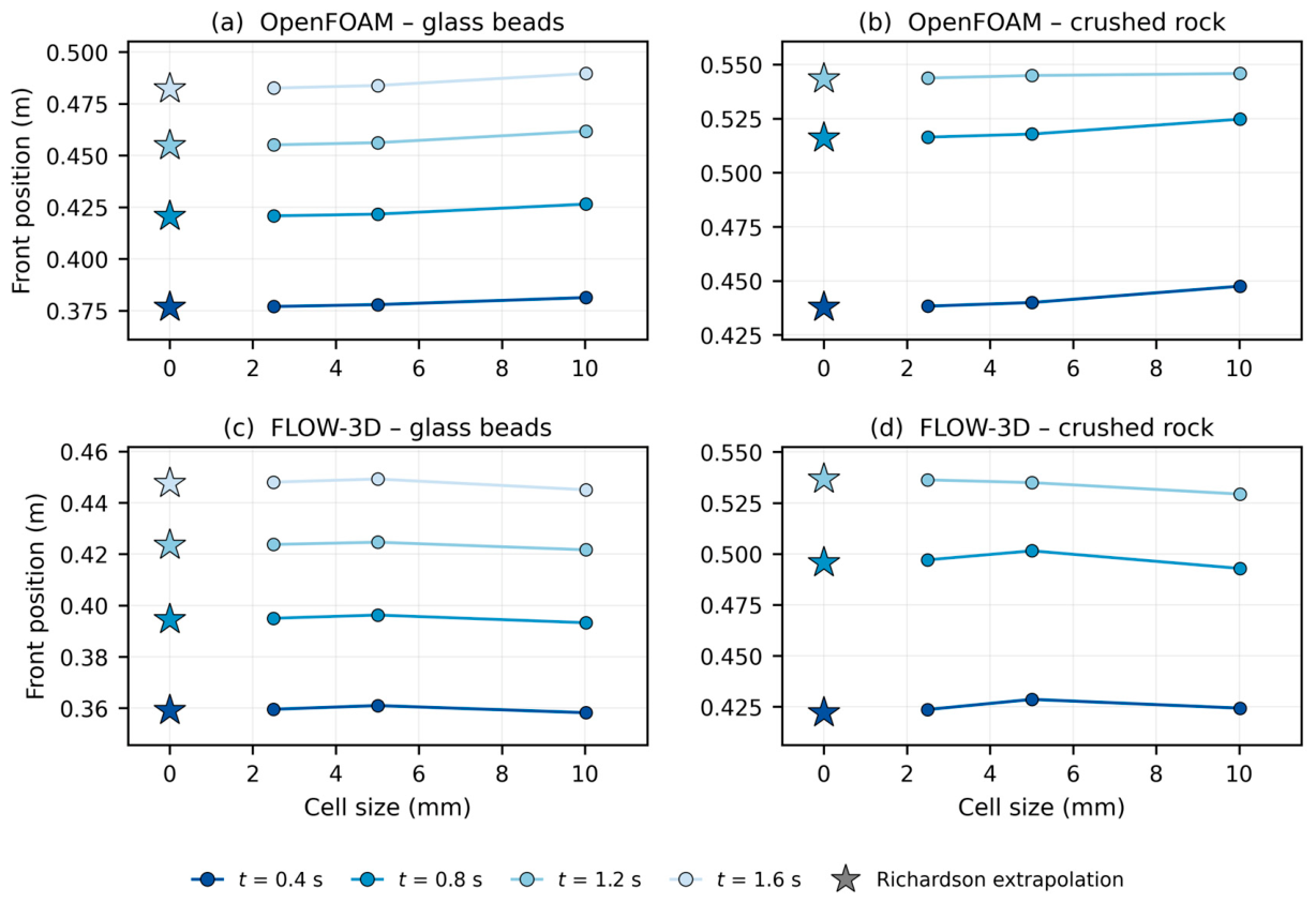
For Experiments 1 and 3, the grid listed there is the middle member of a three-grid sequence on which the discretization error was assessed following Celik et al. [53]. Those two assessments are reported in Appendix B, in Figure A8 for Experiment 1, and in Figure A9 and

Table A4. Points of Experiment 3 at which the three solutions form a monotone sequence, with the observed order of convergence p_obs and the extrapolated value referred to the medium grid.

Model	Quantity	Point	Coarse	Medium	Fine	pobs	Extrapolated	Index (%)
FLOW-3D	ηmax	WG1	0.0923	0.0898	0.0894	7.82	0.0894	0.57
FLOW-3D	ηmax	WG2	0.0922	0.0897	0.0894	8.02	0.0893	0.54
FLOW-3D	ηmax	WG3	0.0985	0.0966	0.0958	3.49	0.0953	1.68
FLOW-3D	ηmax	WG4	0.0980	0.0960	0.0952	4.15	0.0949	1.43
FLOW-3D	ηmax	WG6	0.0910	0.0891	0.0887	7.00	0.0886	0.58
FLOW-3D	ηmax	WG9	0.0711	0.0712	0.0713	7.00	0.0713	0.06
FLOW-3D	ηmax	WG10	0.1059	0.1043	0.1029	1.13	0.0993	5.95
FLOW-3D	ηmax	WG12	0.0641	0.0628	0.0621	2.54	0.0614	2.92
FLOW-3D	ηmax	WG14	0.0940	0.0918	0.0918	16.82	0.0918	0.04
FLOW-3D	ηmax	WG15	0.0941	0.0912	0.0912	16.90	0.0912	0.06
porousWaveFoam	ηmax	WG14	0.0909	0.0938	0.0947	4.54	0.0951	1.67
FLOW-3D	Impulse	P4	660.7	649.9	648.6	8.64	648.5	0.27
porousWaveFoam	Impulse	P1	897.2	1055.2	1086.0	6.10	1093.8	4.57
porousWaveFoam	Impulse	P4	639.4	651.4	661.7	0.55	727.5	14.59
porousWaveFoam	pmax	P1	926.7	1054.1	1084.0	5.40	1093.7	4.69

for Experiment 3, and give the value of 0.03 used for the discretization component of the combined uncertainty. The five cases are presented in turn below, beginning with a check that the wave delivered to the structure is the same in both models.

Table 4. Summary of hydraulic experiments used for model validation.

Experiment	Reference	Case Description
Ex-1	Liu et al. [35]	Porous dam-break flow (glass and rock media)
Ex-2	Lara et al. [54]	Three-dimensional wave interaction with a side-mounted porous caisson
Ex-3	Lara et al. [54]	Three-dimensional wave interaction with a transverse porous caisson
Ex-4	Jensen et al. [55]	Solitary-wave interaction with a porous breakwater slope
Ex-5	Guler et al. [37]	Solitary waves overtopping a rubble-mound breakwater

Table 4. Summary of hydraulic experiments used for model validation.

Experiment	Reference	Case Description
Ex-1	Liu et al. [35]	Porous dam-break flow (glass and rock media)
Ex-2	Lara et al. [54]	Three-dimensional wave interaction with a side-mounted porous caisson
Ex-3	Lara et al. [54]	Three-dimensional wave interaction with a transverse porous caisson
Ex-4	Jensen et al. [55]	Solitary-wave interaction with a porous breakwater slope
Ex-5	Guler et al. [37]	Solitary waves overtopping a rubble-mound breakwater

Table 5. Boundary conditions for Experiment 1.

Boundary	porousWaveFoam			FLOW-3D
	alpha.water	Pressure	Velocity
Atmosphere	inletOutlet	totalPressure	pressureInletOutletVelocity	Pressure (fluid fraction = 0)
Wall	zeroGradient	fixedFluxPressure	fixedValue (0 0 0)	Wall
Front and back	empty
Wave generation	Not applied
Wave absorption

Table 5. Boundary conditions for Experiment 1.

Boundary	porousWaveFoam			FLOW-3D
	alpha.water	Pressure	Velocity
Atmosphere	inletOutlet	totalPressure	pressureInletOutletVelocity	Pressure (fluid fraction = 0)
Wall	zeroGradient	fixedFluxPressure	fixedValue (0 0 0)	Wall
Front and back	empty
Wave generation	Not applied
Wave absorption

Table 6. Boundary conditions for Experiments 2 to 5.

Boundary	porousWaveFoam			FLOW-3D
	alpha.water	Pressure	Velocity
Atmosphere	inletOutlet	totalPressure	pressureInletOutletVelocity	Pressure (fluid fraction = 0)
Inlet	zeroGradient			Solitary wave
Outlet	zeroGradient		inletOutlet	Outflow
Wall	zeroGradient	fixedFluxPressure	fixedValue (0 0 0)	Wall
Wave generation	waves2Foam relaxation zone with Chappelear [39] solitary-wave theory and target velocity imposed through relaxation zone			Built-in solitary-wave boundary
Wave absorption	No separate absorption layer; outgoing flow leaves through the outlet boundary			None; outflow boundary

Table 6. Boundary conditions for Experiments 2 to 5.

Boundary	porousWaveFoam			FLOW-3D
	alpha.water	Pressure	Velocity
Atmosphere	inletOutlet	totalPressure	pressureInletOutletVelocity	Pressure (fluid fraction = 0)
Inlet	zeroGradient			Solitary wave
Outlet	zeroGradient		inletOutlet	Outflow
Wall	zeroGradient	fixedFluxPressure	fixedValue (0 0 0)	Wall
Wave generation	waves2Foam relaxation zone with Chappelear [39] solitary-wave theory and target velocity imposed through relaxation zone			Built-in solitary-wave boundary
Wave absorption	No separate absorption layer; outgoing flow leaves through the outlet boundary			None; outflow boundary

Table 7. Mesh and porous-medium properties of the five benchmark configurations. The coefficients α and β apply to porousWaveFoam only.

Case	Cells, porousWaveFoam	Cells, FLOW-3D	D50 (m)	Porosity n	α/β (porousWaveFoam)
Ex-1	20,648	2,344,163 a	glass 0.003/rock 0.0159	glass 0.39/rock 0.49	1000/2.0
Ex-2	1,553,848	1,557,632	0.0083	0.48	500/2.0
Ex-3	2,568,000	2,480,175	0.015	0.51	1000/3.0
Ex-4	1,944,000	1,947,180	body 0.038/plate 0.0182/zone 0.038	body 0.40/plate 0.41/zone 0.40	500/2.0
Ex-5	3,547,143	3,548,448	filter 0.033/core 0.015/armor 0.040	filter 0.35/core 0.30/armor 0.40	11.375/0.70; 10.5/0.36; 12.0/0.24

^a Experiment 1 is two-dimensional and was run in porousWaveFoam on a one-cell-thick grid, whereas the FLOW-3D setup is three-dimensional. The in-plane cell size is 5.0 mm in both.

Table 7. Mesh and porous-medium properties of the five benchmark configurations. The coefficients α and β apply to porousWaveFoam only.

Case	Cells, porousWaveFoam	Cells, FLOW-3D	D50 (m)	Porosity n	α/β (porousWaveFoam)
Ex-1	20,648	2,344,163 a	glass 0.003/rock 0.0159	glass 0.39/rock 0.49	1000/2.0
Ex-2	1,553,848	1,557,632	0.0083	0.48	500/2.0
Ex-3	2,568,000	2,480,175	0.015	0.51	1000/3.0
Ex-4	1,944,000	1,947,180	body 0.038/plate 0.0182/zone 0.038	body 0.40/plate 0.41/zone 0.40	500/2.0
Ex-5	3,547,143	3,548,448	filter 0.033/core 0.015/armor 0.040	filter 0.35/core 0.30/armor 0.40	11.375/0.70; 10.5/0.36; 12.0/0.24

^a Experiment 1 is two-dimensional and was run in porousWaveFoam on a one-cell-thick grid, whereas the FLOW-3D setup is three-dimensional. The in-plane cell size is 5.0 mm in both.

3.2.1. Incident Wave in the Absence of the Structure

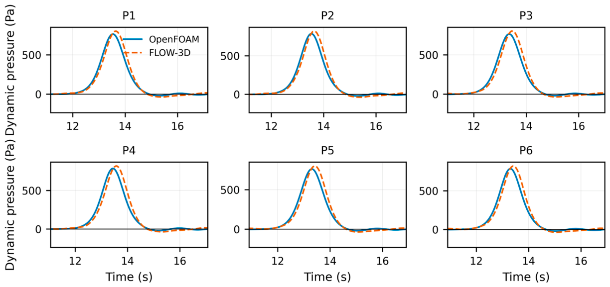
The two configurations generate the solitary wave from different theories, namely Chappelear [39] in porousWaveFoam and McCowan [40] in FLOW-3D, so a difference established at the generation stage would propagate into every subsequent comparison. This was examined in a numerical flume built from the transverse-caisson case, Experiment 3, with the porous structure removed and everything else unchanged. The domain, the mesh, the incident wave and the boundary settings are those listed for that case in Table 6 and Table 7. The wave generated by each model is, therefore, compared under identical conditions. Both are compared against the first-order solitary-wave solution of Equations (17) and (18). The pressure records at the six transducers are given in Figure A7 of Appendix A.

$$\eta \left(x,t\right)=H{sech}^2\left[\sqrt{{\displaystyle \frac{3H}{4h^3}}\left(x-ct\right)}\right]$$

(17)

$$c=\sqrt{g(h+H)}$$

(18)

In these expressions, $H$ is the solitary-wave height, $h$ is the still-water depth, $x$ and $t$ are the spatial and temporal coordinates, and $g$ denotes the gravitational acceleration.

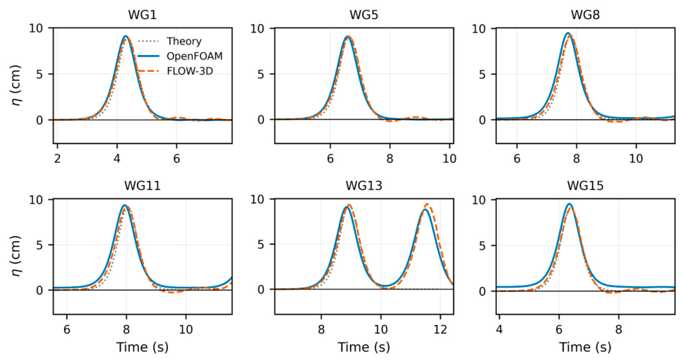
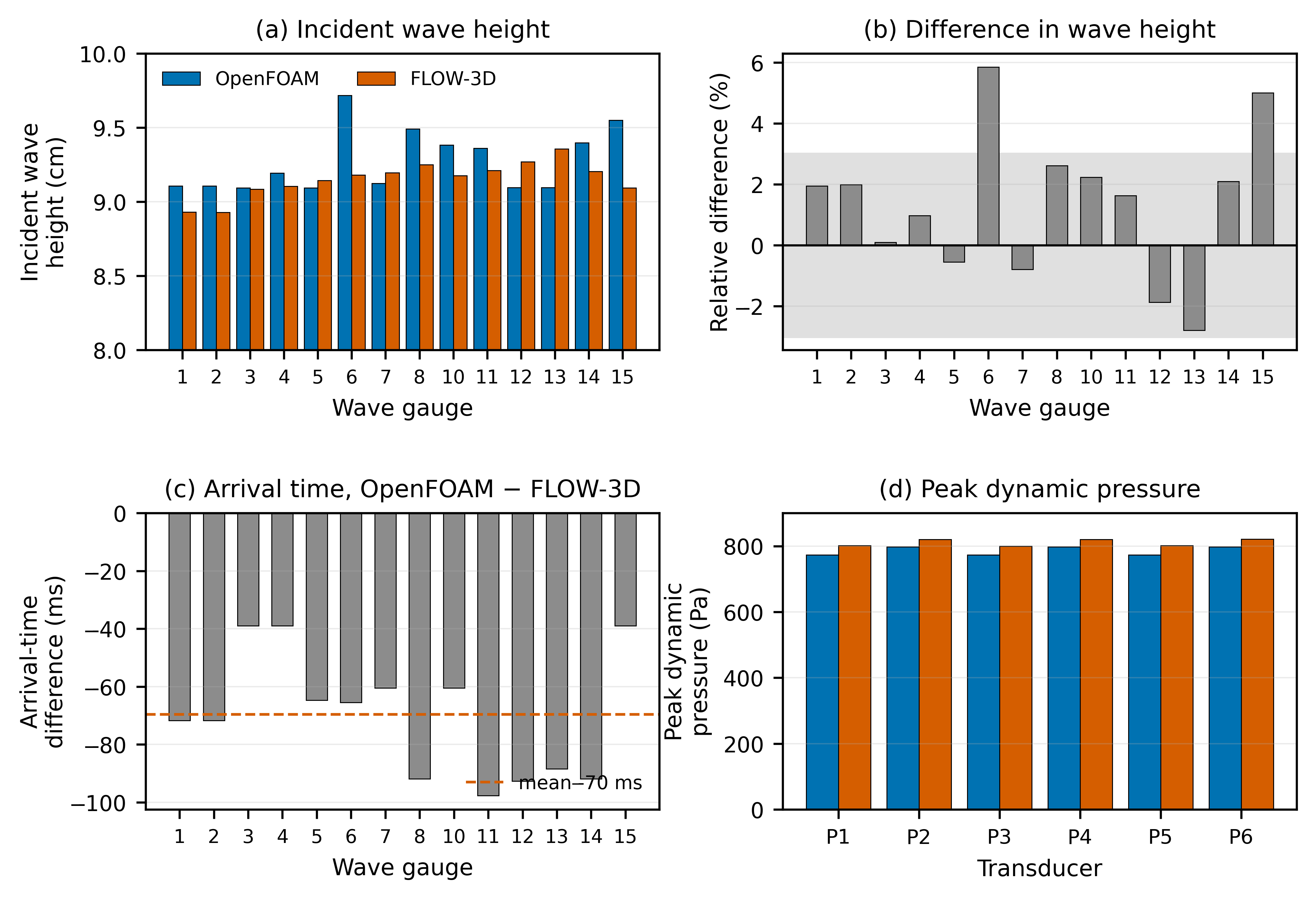
Both configurations reproduce the theoretical solitary-wave profile at every gauge (Figure 1). The incident wave height differs by 1.3% on average across the gauges, with a standard deviation of 2.4%, and the cross-correlation between the two records is 0.991 with an amplitude ratio of 0.991 and a normalized RMSE of 0.038. Arrival time was taken as the instant of the first-pass crest at each gauge, and the wave generated by porousWaveFoam arrives 70 ms earlier on average, with a between-gauge scatter of 21 ms. The dynamic pressure agrees to a similar degree. Once the hydrostatic component is removed, the peak values at the six transducer locations differ by 2.7 to 3.5% consistently in the same direction (Figure 2).

The two models, therefore, deliver the same incident wave to within 1.3% in height, 0.038 in normalized RMSE, and 70 ms in arrival time, and the pressure signal to within 3.5%. These values are the resolution floor of the comparison; a difference of this size between the two models, measured in a case that contains a structure, cannot be attributed to the structure. Differences larger than the floor are interpreted in the following subsections as arising from the interaction with the structure.

3.2.2. Porous Dam-Break Flow (Glass and Rock Media)

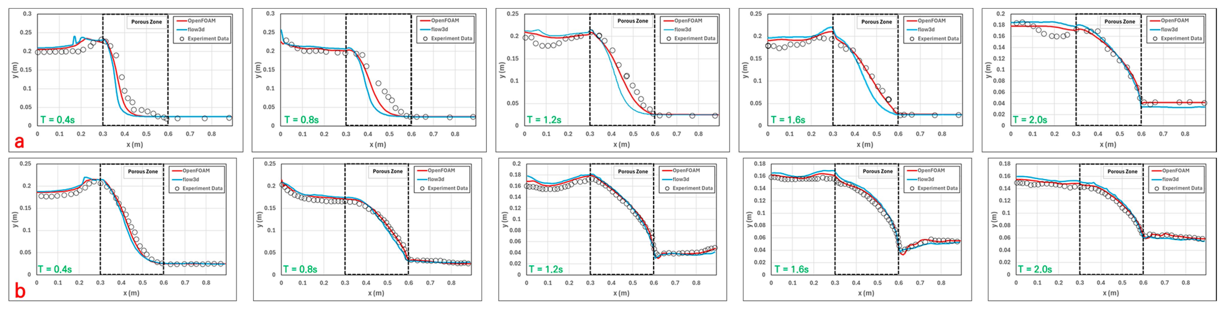
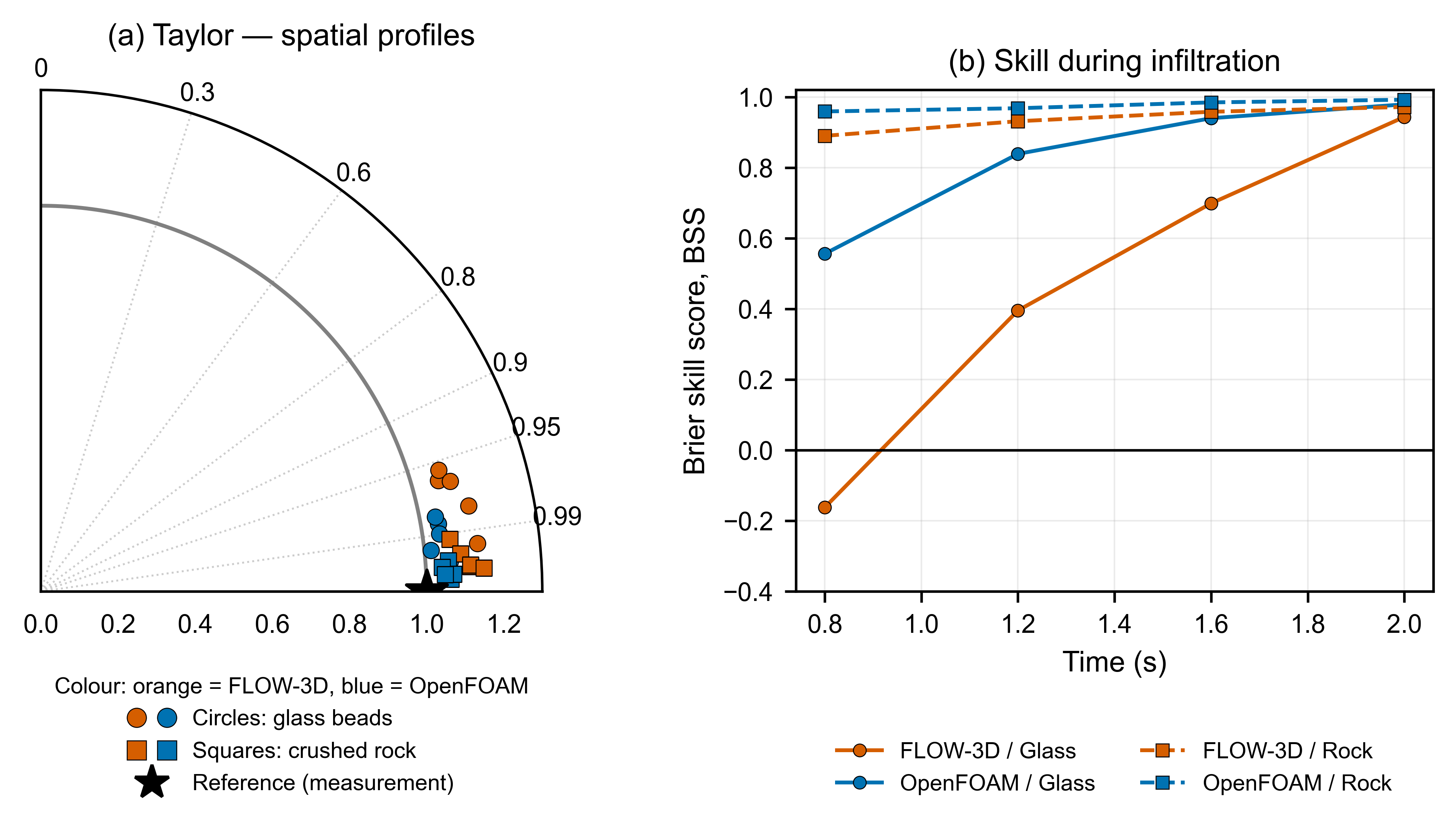
To assess model performance for unsteady free-surface flow through porous media, the porous dam-break experiment of Liu et al. [35] was reproduced for two contrasting media: small spherical glass beads and crushed rock. Because the available data consist of spatial free-surface profiles at discrete snapshots rather than continuous time histories, the comparison was based on the profile-derived error components summarized in Figure 3. The measured and simulated free-surface profiles for both media are given in Figure A1 of Appendix A.

porousWaveFoam reproduces the free-surface profile more closely than FLOW-3D in both media, and the advantage lies almost entirely in the amplitude component. FLOW-3D over-predicts the spread of the profile, its amplitude ratio being 1.10 in both media against 1.04 and 1.06 for porousWaveFoam. The two agree on waveform shape to within 0.002 in correlation for the rock. Because the profiles are spatial snapshots rather than time series, no timing component is available here. The difference between the models is larger in the glass beads, where the flow is more strongly resistance-controlled. The normalized RMSE differs by 0.043 there against 0.017 in the coarser rock.

The compared quantity in this benchmark is a spatial profile rather than a time series. The shift component of the decomposition, therefore, has the dimension of length and can be read directly as the error in the position of the infiltration front. Both models advance the front further than measured over the first part of the infiltration, and FLOW-3D consistently more than porousWaveFoam. In the glass-bead medium, the offset reaches 6.2 cm for FLOW-3D and 4.0 cm for porousWaveFoam at t = 0.8 s. These correspond to 4.5 and 2.9 cell widths, well above the resolution at which the shift can be determined. In the crushed-rock medium, the corresponding maxima are 2.4 cm and 1.3 cm, and by t = 1.6 s, both fall below one cell width. The offsets of the two models converge to within 0.6 cm by t = 2.0 s in both media. Expressed as a length, the shift component, therefore, places the disagreement in the early stage of the infiltration, when the front advances fastest, and shows it to be larger in the finer of the two media. The complete set of values is given in

Table A1. Front-position offset in the porous dam-break benchmark (Experiment 1). Negative values indicate that the modeled front leads the measurement.

Medium	Time (s)	Offset, OpenFOAM (m)	Offset, FLOW-3D (m)	Offset/Cell, OF	Cell Width (m)
Glass beads	0.4	−0.0231	−0.0367	−1.7	0.0132
	0.8	−0.0396	−0.0615	−2.9	0.0137
	1.2	−0.0265	−0.0538	−1.9	0.0137
	1.6	−0.0120	−0.0412	−0.9	0.0130
	2.0	+0.0006	−0.0010	+0.0	0.0136
Crushed rock	0.4	−0.0134	−0.0236	−1.1	0.0125
	0.8	−0.0045	−0.0211	−0.5	0.0086
	1.2	−0.0033	−0.0058	−0.4	0.0084
	1.6	−0.0001	+0.0029	−0.0	0.0078
	2.0	+0.0049	+0.0061	+0.5	0.0090

of Appendix B.

This is the first instance of the conditional behavior seen across the benchmarks. The two models receive the same grain diameter and porosity, and the two media differ only through those two inputs, so the margin between the models here reflects how each converts them into resistance. That margin is smaller for the crushed rock, whose linear resistance is roughly two orders of magnitude below that of the glass beads. In this benchmark, the choice of model, therefore, has the greater effect in the finer medium, where the resistance term carries the larger share of the momentum balance.

3.2.3. Three-Dimensional Wave Interaction with a Side-Mounted Porous Caisson

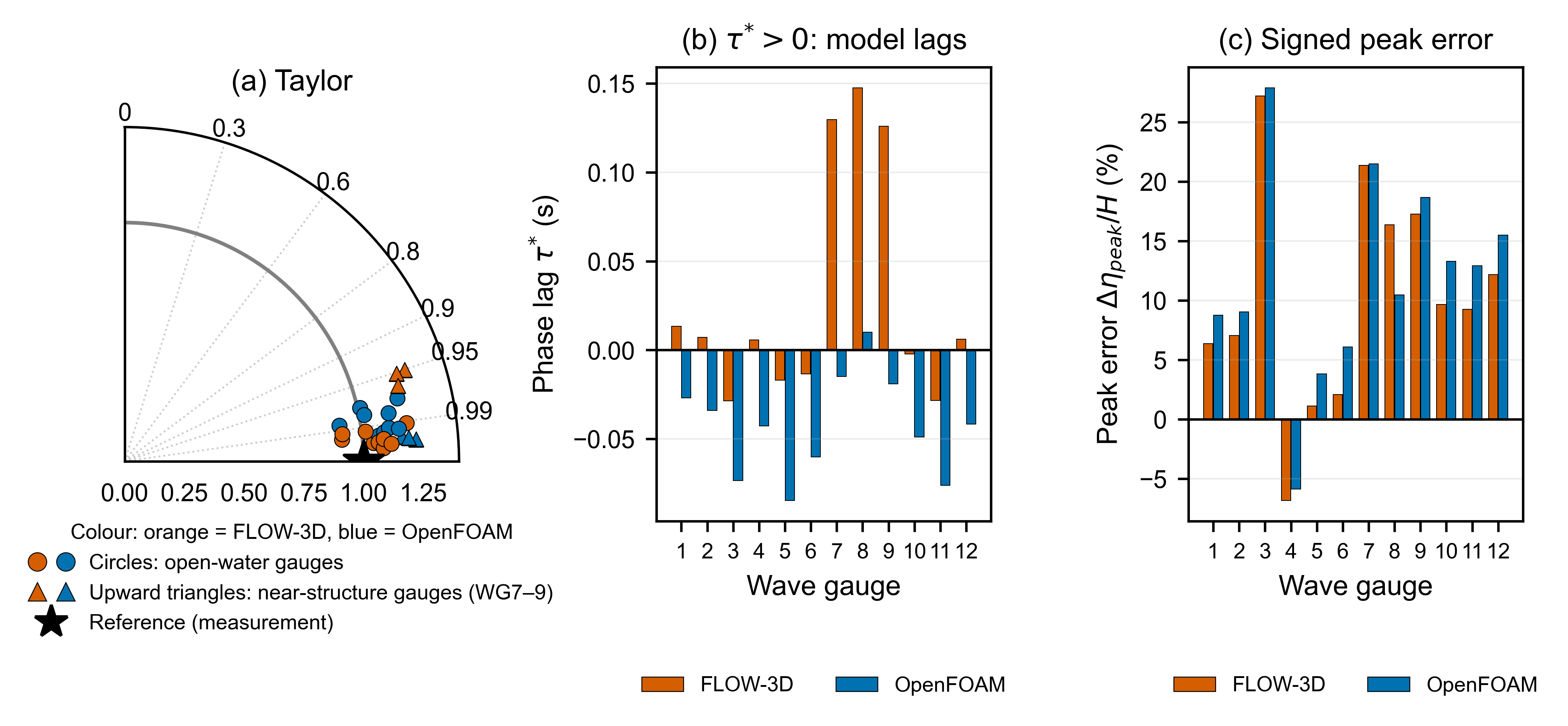
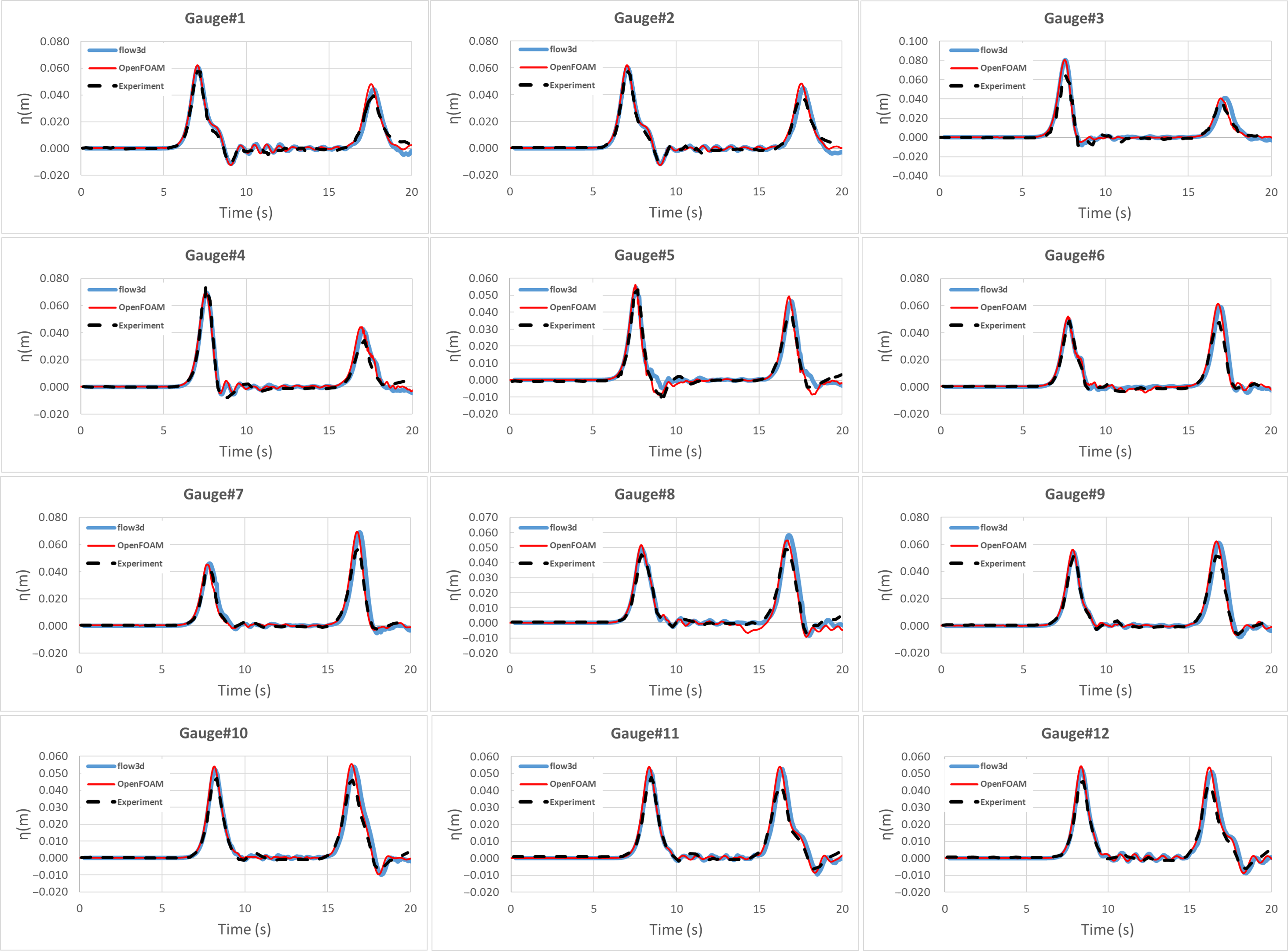
To evaluate the reproduction of three-dimensional free-surface propagation past a side-mounted porous caisson, the wave-basin experiment of Lara et al. [54] was reproduced and the free-surface time series at twelve wave gauges were compared using the decomposed error components (Figure 4). The records at all twelve gauges are given in Figure A2 of Appendix A.

Across the twelve gauges, neither model is uniformly superior, and a paired bootstrap over all gauges finds no error component whose mean porousWaveFoam–FLOW-3D difference is separated from zero by more than the resampling interval. For the peak error, the component with the largest mean difference, the twelve-gauge mean is +0.016 with a 95% resampling interval of [−0.001, +0.028] from 10,000 resamples. As set out in Section 3.1, that interval describes the scatter across the observed gauge set rather than serving as an inferential test. The component-wise decomposition instead shows a zone-dependent reversal. In the open-water gauges, the two models agree closely, FLOW-3D matching the peak amplitude marginally better and carrying essentially zero phase lag. Immediately adjacent to the structure, at WG7 to WG9, the ranking reverses. FLOW-3D develops a positive phase lag of ${\tau }^{*}$ = +0.134 s on average, and its zero-lag correlation falls to $R$ = 0.955. porousWaveFoam keeps a lag of −0.008 s with $R$ = 0.997 and a lower normalized RMSE, 0.077 against 0.131.

The digitized records in this zone are sampled at 0.079 s on average, so a lag is only meaningful when it exceeds that interval. The FLOW-3D lag is 1.7 times the sampling interval and is, therefore, resolved, whereas the porousWaveFoam lag is an order of magnitude below it and is reported as zero. Six of the twenty-four gauge-model combinations in this experiment return a resolvable lag, and the three FLOW-3D near-structure gauges are among them. What separates the two models near the structure is when the wave arrives, not what it looks like when it does. The shift-optimized shape correlation is 0.997 for both, so the whole of the FLOW-3D correlation deficit is removed by sliding its record 0.134 s earlier. The waveform is reproduced, but too late. Numerical diffusion would not act this way, since it would flatten the crest and lower the shape correlation as well. What the components locate is, therefore, a difference in propagation speed close to the caisson rather than a loss of resolution, and the difference appears only in that zone. FLOW-3D carries no lag in open water.

The practical consequence follows from which quantity a design check uses. Peak elevation is unaffected. Both models over-predict the near-structure crest by a similar margin, 17% for porousWaveFoam and 18% for FLOW-3D, and either may be used for that purpose. A check that depends on when the crest arrives, such as the phasing of overtopping against a water-level condition, would carry the 0.134 s offset of FLOW-3D in this zone. The ranking of the two models in this three-dimensional case is thus a function of both the spatial zone and the quantity asked of it, which a single averaged error would not show.

3.2.4. Three-Dimensional Wave Interaction with a Transverse Porous Caisson

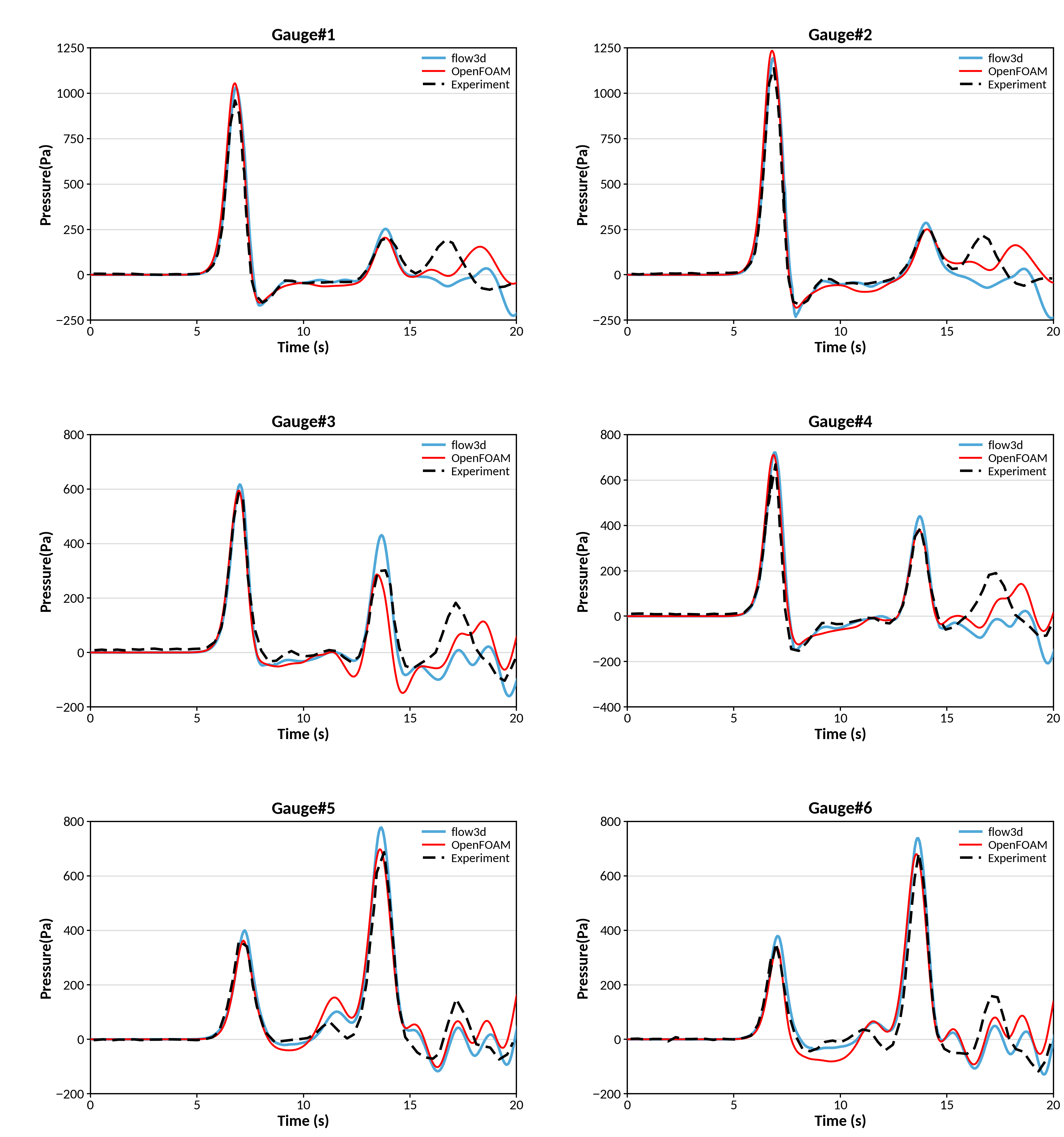
To evaluate the numerical models for three-dimensional wave interaction with a transverse porous caisson, the wave-basin experiment of Lara et al. [54] was reproduced. Free-surface elevations were compared at multiple wave gauges, and wave-induced pressures were compared at six transducers on the front face of the porous structure. The water-level records are given in Figure A3 of Appendix A and the pressure records in Figure A4. A three-grid convergence assessment was carried out for this case and is reported in Appendix B.2. Together with Experiment 1, it covers the two ways in which the flow is set in motion in this study. In Experiment 1, the motion originates from an initial water column released at rest. Here, it is introduced through the wave-generation boundary and travels the length of the flume before reaching the structure. The discretization error of a case, therefore, depends on which of the two applies, and one case of each type was assessed. Pressure was chosen for that assessment because the design scalars of this benchmark are derived from it.

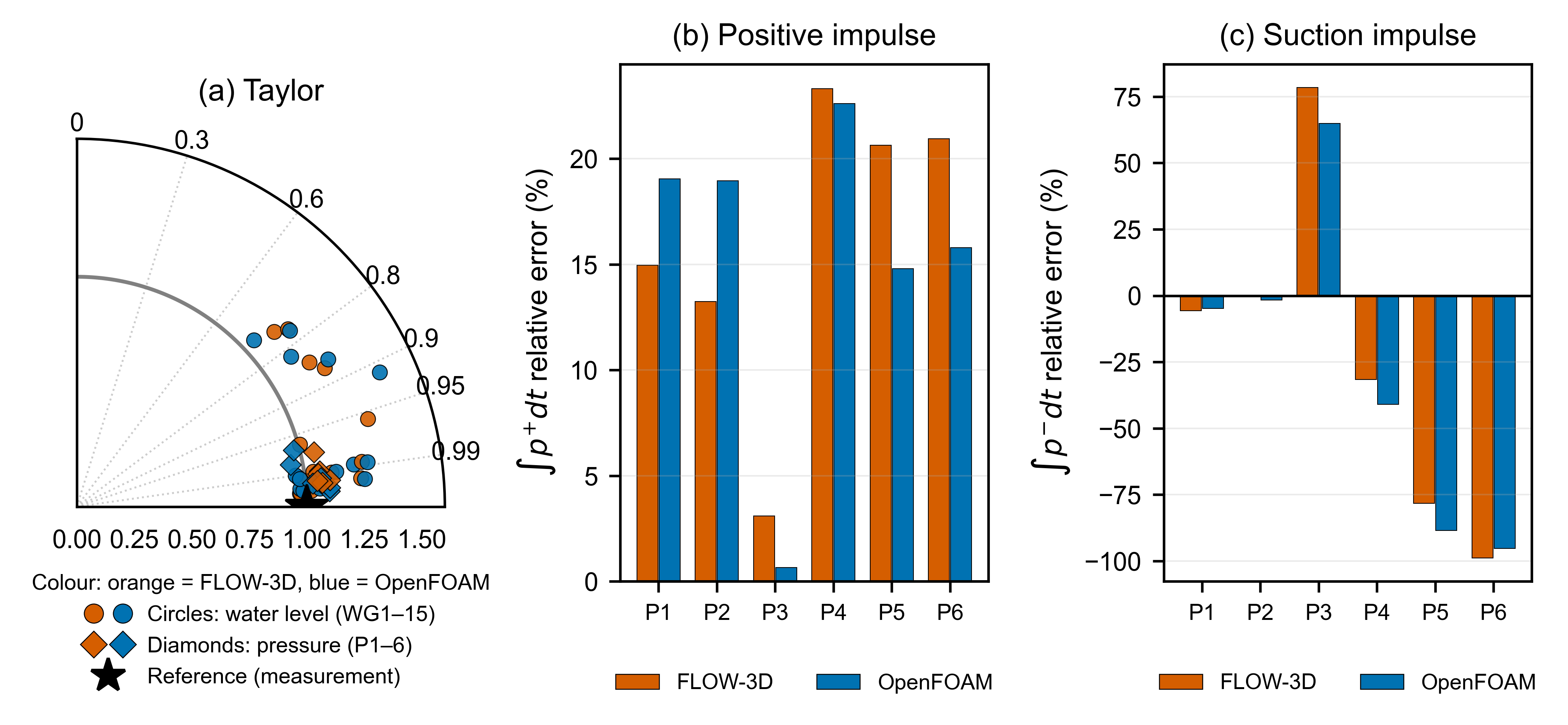
Both models reproduce the free-surface elevation and the pressure arrival with broadly comparable skill. On the Taylor diagram of Figure 5a, the two sets of points fall close together throughout. Averaged over the six transducers, the pressure signal gives a correlation of 0.989 for both models, with amplitude ratios of 1.04 and 1.07. The water level is reproduced with a correlation of 0.987 at the gauges away from the caisson and 0.80 at those beside it. The accuracy of both models, therefore, falls in the same place, where the incident and reflected waves overlap. What the elementary components do not do is separate the two models. At no gauge or transducer does either lead by more than the combined uncertainty.

The design scalars, however, reveal a spatial reversal in the pressure response. The cumulative positive impulse is over-predicted by both models at every front-face transducer, but the model with the larger error changes with the height. The porousWaveFoam over-predicts most strongly at the lower points P1 and P2, by 19.0% against 14.1%, whereas FLOW-3D does so at the upper points P3 to P6, by 17.0% against 13.5%. Neither is uniformly conservative across the face of the structure. The lower-face difference exceeds the combined uncertainty by a factor of 1.6 and the upper-face difference by 1.1, so the reversal between the two zones is resolved by the test of Section 3.5. The upper-face margin is narrow enough, however, to depend on the discretization uncertainty adopted there. It carries a practical consequence. A designer checking the load on the lower part of the face obtains the more conservative estimate from porousWaveFoam, and one checking the upper part obtains it from FLOW-3D. No single choice of model is conservative over the whole face.

The suction impulse integrates the interval in which the pressure falls below the still-water value, which occurs as the crest passes and the water surface drops back down the face. It measures the outward load that acts on the structure during that interval, and it behaves quite differently from the positive impulse.

The error follows the height of the transducer. At the two lowest points, which stay submerged throughout the event, both models reproduce the suction to within 5%. From P4 upward, the modeled suction falls progressively short of the measurement, by 32 to 41% at P4, by 78 to 89% at P5, and by 95 to 99% at P6. At the top of the face, almost none of the measured outward load is recovered. The transducers that lose the suction are those the free surface crosses as the crest passes. The single exception is P3, where both models over-predict the suction by 65% and 78%. The measured negative area at that transducer is small, so the relative error there is amplified and the value is not read as a distinct behavior. 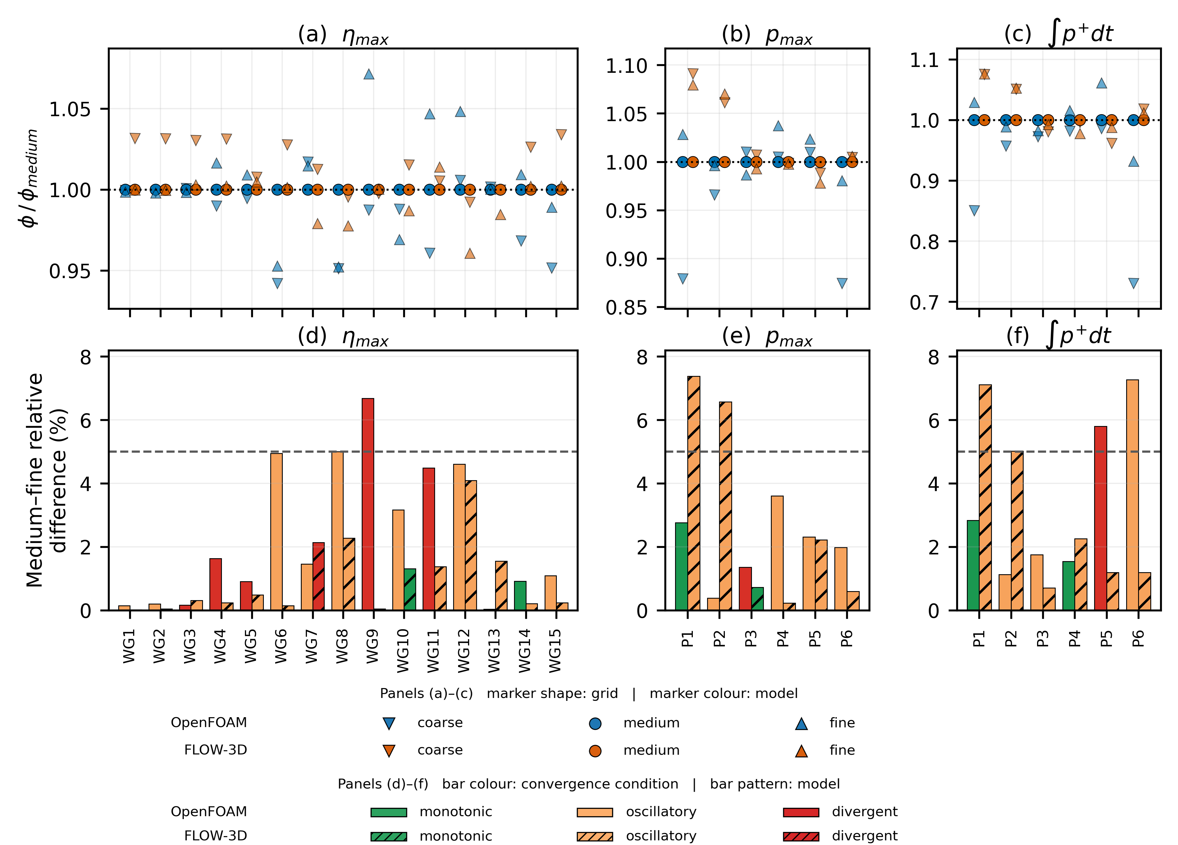The two models are separated at neither the lower nor the upper face, the difference falling inside the combined uncertainty in both zones (Section 3.5). The shortfall is, therefore, shared, and changing the model does not remove it. Its extent is set by the position on the face. The suction is reproduced where the transducer stays submerged and is lost where the free surface crosses it. The positive impulse gives no warning of this, since both models reproduce it at the same upper transducers to within 21%, so a validation reported only in that quantity would record the upper face as satisfactory. The limitation is common to both models and confined to the part of the face that emerges during the event, so a suction taken from either model there should be read as a lower bound on the outward load.

3.2.5. Solitary-Wave Interaction with a Porous Breakwater Slope

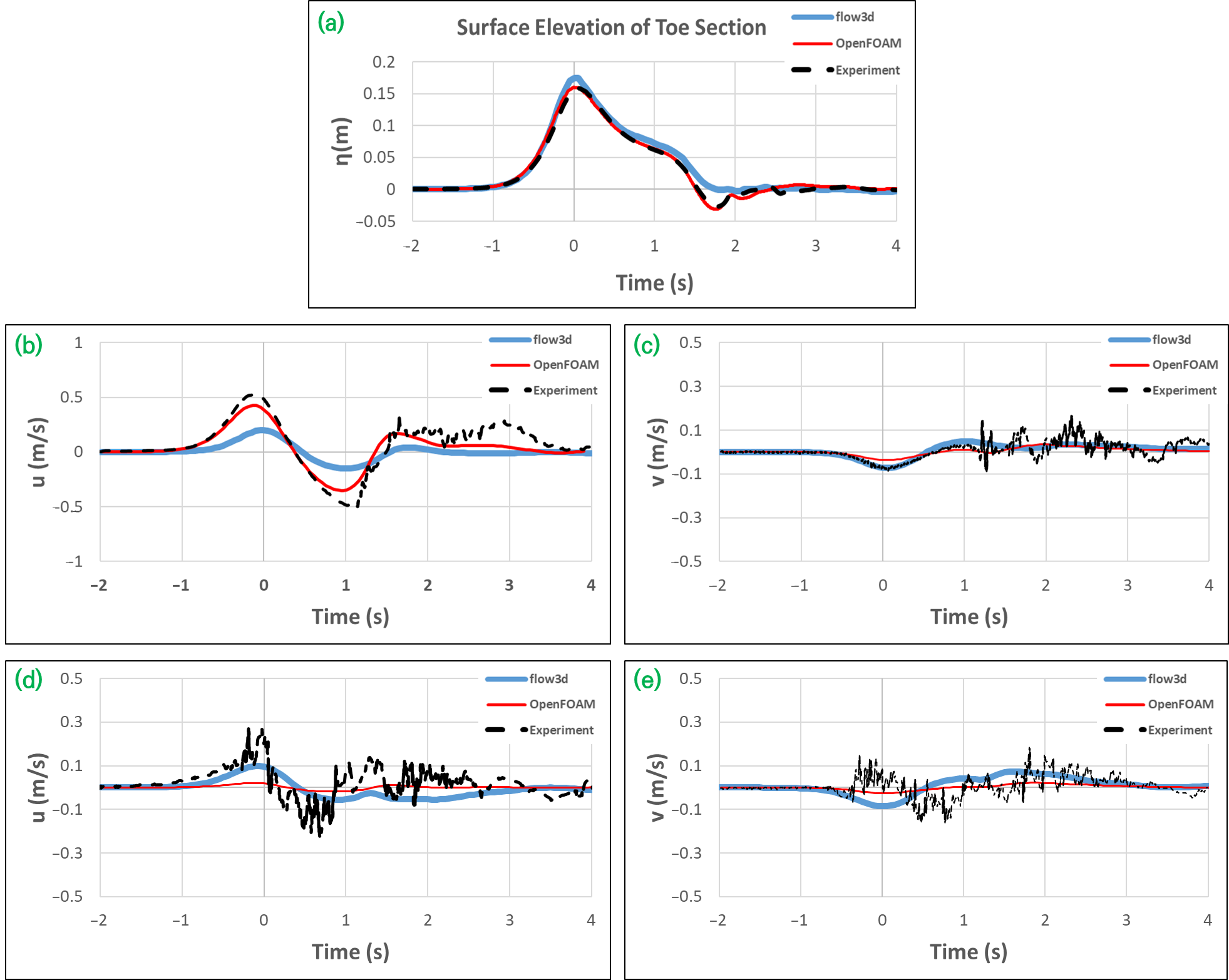
To validate the reproduction of free-surface run-up and slope-parallel and slope-normal velocities on a porous breakwater slope, the experiment of Jensen et al. [55] was reproduced. Free-surface elevation at the toe and the slope velocity components were compared using the decomposed error components and the design scalars (Figure 6). The toe-elevation and slope-velocity records are given in Figure A5 of Appendix A.

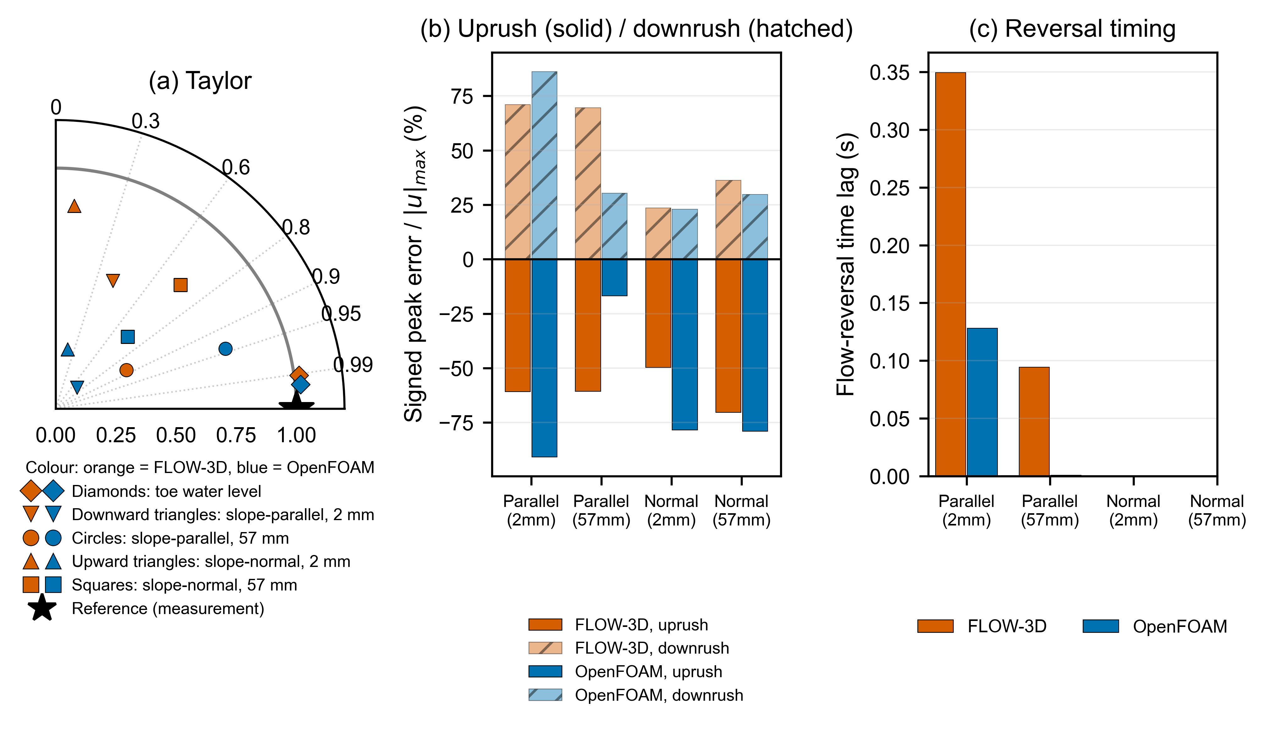
For the free-surface family, porousWaveFoam reproduces the toe elevation with smaller amplitude and shape errors than FLOW-3D (NRMSE 0.030 vs. 0.059). The velocity family behaves differently, and in a way that matters more for design. The two models share the same directional error. Both models damp the peak slope velocity. On the way up, they under-predict the positive peak. On the way down, they return a peak too weak in magnitude. That is, algebraically higher than the measured negative peak. The signed peak-velocity error, normalized by the peak measured speed of each record, is, therefore, negative in uprush and positive in downrush for both models. At the measurement point 57 mm from the slope surface, it ranges from −17% to −79% in uprush and from +30% to +70% during downrush. Its sign is set by the motion phase rather than by the choice of model, and the same holds for both velocity components. The magnitudes differ between the models and change order with the component. During uprush, porousWaveFoam under-predicts the slope-parallel velocity by 17%, against 61% for FLOW-3D, and the slope-normal velocity by 79% against 70%.

The two measurement distances behave differently. At 57 mm, both models follow the measured signal with zero-lag correlations of 0.71 to 0.94, whereas at 2 mm, the correlation of the slope-normal component falls to 0.09 and 0.20. And no flow-reversal instant can be extracted. Scalars from the 2 mm records are, therefore, reported but not used to rank the models.

Two features of this case bear on model selection. The first is that the free-surface response and the velocity response are not equally well-reproduced. The toe elevation is captured to within 3% in normalized RMSE, whereas the slope velocity is damped by tens of percent at every point. A validation carried out on water level alone would not reveal this. The second is that the velocity error keeps the same sign in both models, so a change of model shifts its magnitude but not its direction, and the damping remains. Since the two configurations differ in their treatment of the air phase and of turbulence (Table 1), the error is not attributable to either of those elements. What they share is the volume-averaged porous closure and the cell-averaged sampling of velocity, which the present comparison cannot separate. For design use, the practical reading is that a slope velocity taken from either model at this scale should be treated as a lower bound.

3.2.6. Solitary Waves Overtopping a Rubble-Mound Breakwater

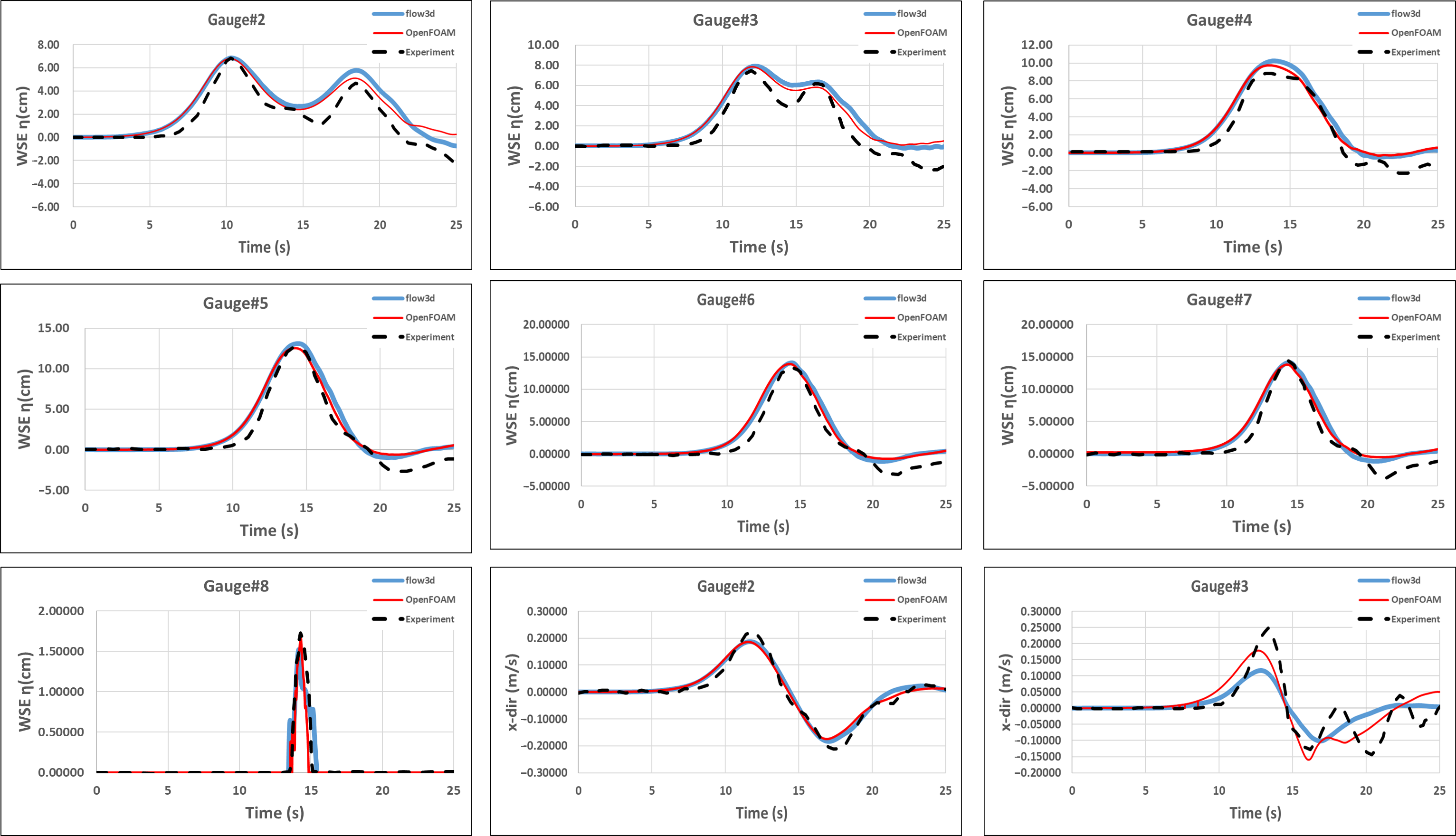
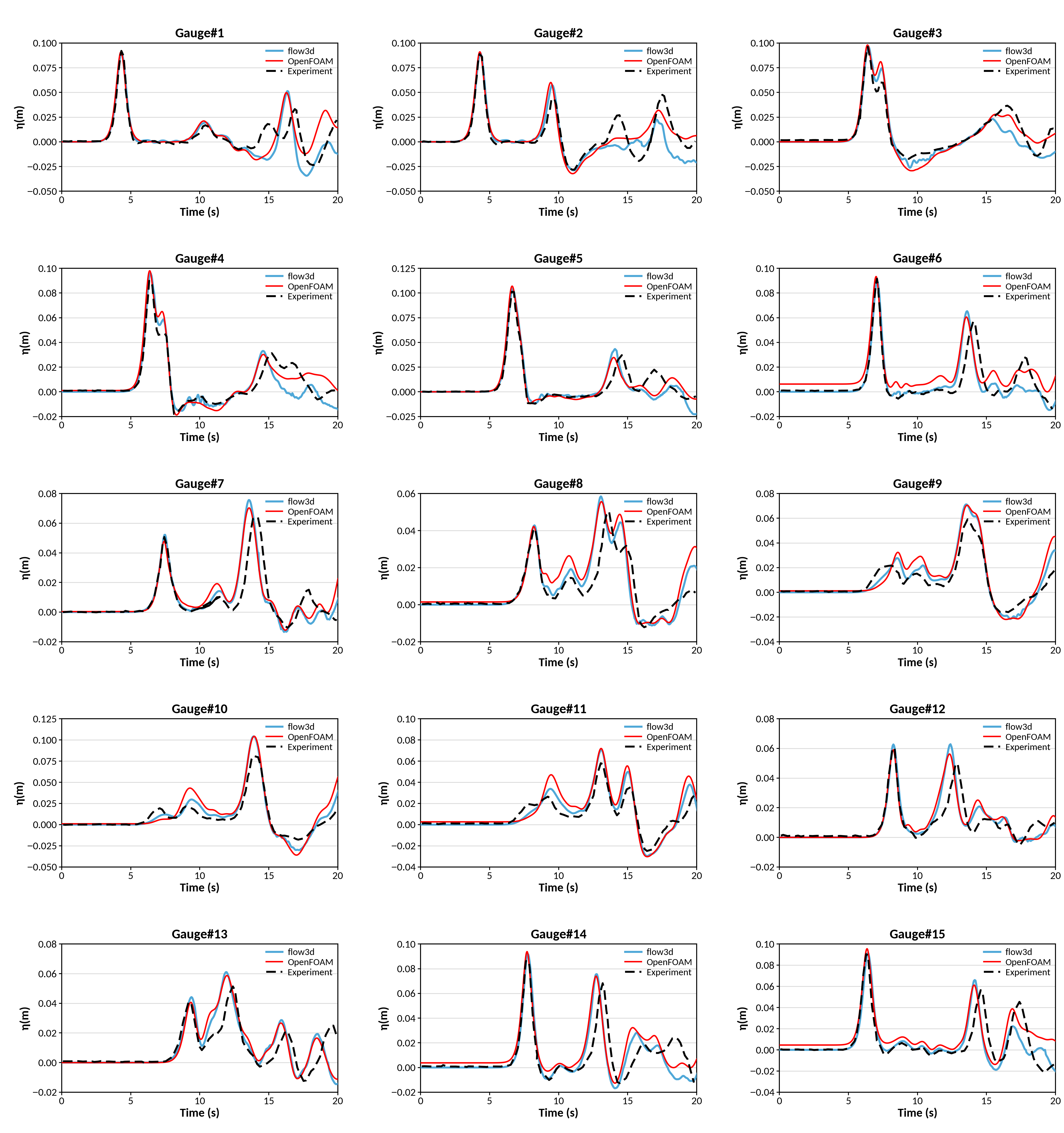
To validate the models for overtopping over a rubble-mound breakwater, the experiment of Guler et al. [37] was reproduced, and the free-surface elevation at seven wave gauges and the velocity at two measurement points were compared using the decomposed error components (Figure 7). The free-surface and velocity records are given in Figure A6 of Appendix A.

The layer-specific resistance coefficients reported for this case by Guler et al. [37] are given in the Engelund-type closure [56] rather than the van Gent closure implemented here. The two differ only in the porosity exponent of the linear term, so requiring both to yield the same linear resistance gives $\alpha \left(\mathrm{v}\mathrm{G}\right)=\alpha \left(\mathrm{E}\right)·n(1-n)$, while the non-linear coefficient transfers unchanged. Table 7 lists the converted values. They are an order of magnitude smaller than those of the other benchmarks because the source study reports a correspondingly lower resistance for these layers, not because a different closure form is used.

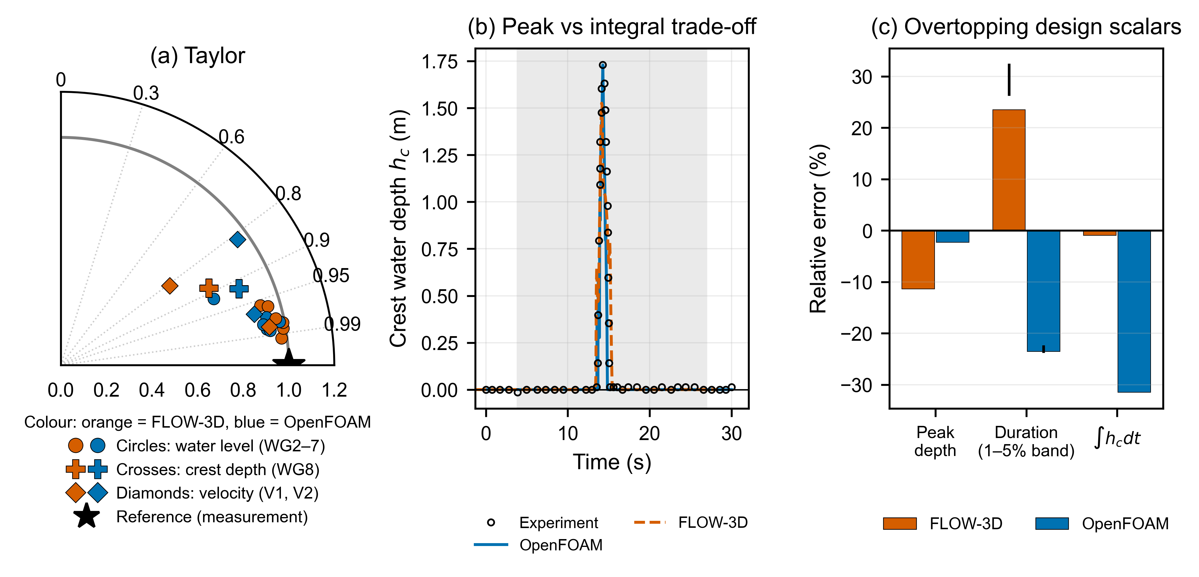
For the water-surface family, WG2 to WG7, the two models are close and mixed rather than uniformly ranked. FLOW-3D reproduces the wave amplitude more faithfully at every gauge, with its ${\sigma }^{*}$ lying nearer unity, whereas porousWaveFoam matches the waveform shape slightly better, with the higher shape correlation at five of the six gauges. The normalized RMSE is comparable, so neither model is clearly superior for the incident and reflected a free surface.

The decisive difference appears in the overtopping response itself, measured at the crest gauge above the crown wall, where the two models trade places between design scalars of the same event. The porousWaveFoam reproduces the peak crest depth almost exactly, at −2.3%, but under-predicts the time-integrated crest depth by 31.5%. FLOW-3D under-predicts the peak depth by 11.4% yet matches the same integral to within 0.9%, at the cost of over-predicting the event duration by 23.5% at a 2% threshold. That figure ranges from 26.5% to 32.3% as the threshold varies between 1% and 5%. The velocity comparison is likewise mixed, both models under-predicting the peak but FLOW-3D more severely at the inner point, by 53% against 28%.

The two errors are not independent. The integral is the product of a depth and a duration. The agreement of FLOW-3D, therefore, follows from a lower crest depth spread over a longer event and the shortfall of porousWaveFoam from a correct depth confined to a shorter one. The free-surface records identify the same behavior upstream. The porousWaveFoam damps the wave amplitude more strongly, with its mean amplitude ratio being 0.90 against 0.96, and delivers the crest 0.18 s earlier. The wave that reaches the crown wall in porousWaveFoam is thus a faster and steeper one, which reproduces the instantaneous depth but drains before the measured event has ended.

The choice of model, therefore, follows the governing design quantity. Where an admissible overtopping limit is expressed as a peak depth on the crest, porousWaveFoam is the closer of the two. Where it is expressed as a volume per unit width, FLOW-3D is, once the crest-depth integral has been converted to a volume by a representative crest velocity.

3.3. Computational-Cost Analysis

Beyond predictive accuracy, the choice between the two models also depends on the computational effort each requires to reach a solution. The two models were executed on different machines, whose specifications are listed in

Table A3. Hardware specification of the two machines used for the cost comparison.

Item	porousWaveFoam Machine	FLOW-3D Machine
Processor	Intel Core i7-8700	AMD Ryzen Threadripper PRO 7985WX
Physical cores/used	6/6	64/64
Base clock	3.2 GHz	3.2 GHz
PassMark single-thread rating	2625	3954
Memory modules	2 × 8 GB	8 × 32 GB
Memory type	DDR4-2666	DDR5-5600, configured at 5200 MT/s
Populated channels	2	8
Total capacity	16 GB	256 GB
Theoretical peak bandwidth	42.7 GB/s	332.8 GB/s
Bandwidth per core used	7.11 GB/s	5.20 GB/s
Operating system	Linux	Windows
Parallel execution	6 MPI subdomains	1 MPI rank × 64 OpenMP threads
Measured parallel efficiency	not recorded	82% (Experiment 2)

, so a comparison based on raw wall-clock time alone would reflect the hardware rather than the models. The cost of each run is, therefore, reported in two forms: the raw wall-clock time-to-solution and a hardware-normalized cost. The resource use of a run is first expressed as core hours (CH), defined as $CH={\displaystyle \frac{t_{wall}\times N_{cores}}{3600}}$, where $t_{wall}$ is the elapsed wall-clock time and $N_{cores}$ the number of cores used. To account for the per-core performance gap between the two hardware generations, a single-thread performance ratio (PR) is defined from the PassMark single-thread rating S as $PR={\displaystyle \frac{S}{S_{ref}}}$ [57], with the porousWaveFoam machine taken as the reference (PR = 1). The normalized core-hours (BNCH) are then $BNCH=CH\times PR$. This places the two runs on a common per-core-performance basis; it does not resolve parallel-scaling efficiency or memory-system differences and is, therefore, used as a practical hardware-aware cost indicator rather than a formal HPC benchmark. For every experiment, both models were advanced to the same physical duration, so the reported costs correspond to an equivalent amount of simulated wave action.

Scaling by a single-thread rating corrects along the processor axis only. Finite-volume CFD of the present type performs few arithmetic operations per quantity loaded from memory, so its throughput is governed as much by the sustainable memory bandwidth of the machine as by processor speed. The roofline model classifies this regime as memory bound [58]. It is also why the STREAM benchmark was introduced, with processor ratings alone having failed to explain the performance differences observed between machines in large-scale ocean modeling [59]. Both raw and normalized figures are, therefore, reported together with the full hardware specification, following Hoefler and Belli [60].

The memory configurations of the two machines differ substantially, and in a way that is not captured by the processor rating. The porousWaveFoam machine carries two DDR4-2666 modules on two channels, giving a theoretical peak bandwidth of 42.7 GB/s; the FLOW-3D machine carries eight DDR5 modules on eight channels operating at 5200 MT/s, giving 332.8 GB/s. The aggregate bandwidth of the second machine is thus 7.8 times the first. Per core, however, the ordering reverses: 7.11 GB/s per core against 5.20 GB/s per core, so that, on the axis most relevant to a memory-bound model, the FLOW-3D machine provides 27% less capability per core, not more. Normalizing by memory bandwidth per core would, therefore, give a performance ratio of 0.73 in place of the 1.51 obtained from the single-thread rating. The two axes disagree by a factor of 2.1, and the value appropriate to a memory-bound model lies between them. Differences in normalized cost smaller than this factor are consequently not interpreted here.

Two features of the FLOW-3D runs work against it on the normalized measure. It solves two additional turbulence transport equations at every step, which porousWaveFoam does not, so the cost reported for it is, if anything, conservative. The normalization also uses the nominal core count of 64, whereas the run for Experiment 2 accumulated 49,726 s of processor time against 944 s elapsed, an efficiency of 82% or 52.7 effective cores. The core hours reported for FLOW-3D are, therefore, an upper bound on the resources actually consumed.

Table 8. Wall-clock time and benchmark-normalized core-hours (BNCH), reported under both performance ratios defined in Section 3.3.

Case	t_wall, OF (s)	t_wall, F3D (s)	BNCH, OF	BNCH, F3D (PR = 1.51)	BNCH, F3D (PR = 0.73)
Ex-1 (glass)	477	409	0.80	10.95	5.32
Ex-1 (rock)	45	367	0.07	9.83	4.77
Ex-2	45,528	944	75.88	25.28	12.28
Ex-3	34,145	2263	56.91	60.60	29.43
Ex-4	23,047	1393	38.41	37.30	18.11
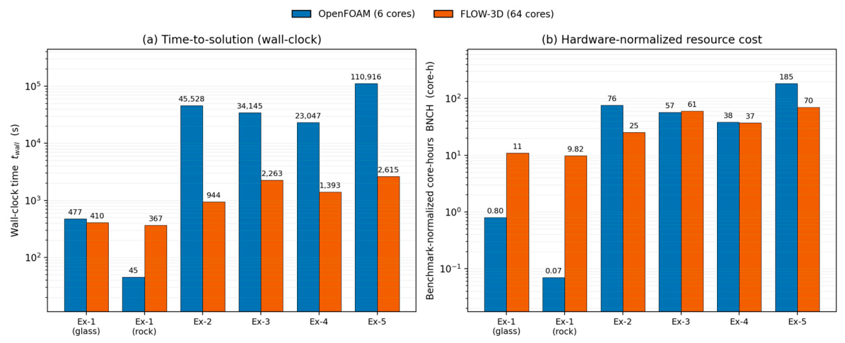
Ex-5	110,916	2615	184.86	70.03	34.00

and Figure 8 summarize the two cost measures across the five benchmarks. In wall-clock time, FLOW-3D reaches the solution faster on all but the smallest problems, by about 48 times for Experiment 2 and 42 times for Experiment 5, reflecting its use of 64 cores. On the hardware-normalized measure, the ranking is mixed, and Table 8 reports it under both normalizations so that the effect of that choice is visible. The porousWaveFoam is more economical for the small dam-break cases of Experiment 1, by factors of 14 and 140 under the processor-based normalization and 7 and 68 under the bandwidth-based one. FLOW-3D is more economical for the larger three-dimensional cases of Experiments 2 and 5, by factors of 3.0 and 2.6 under the first normalization and 6.2 and 5.4 under the second. Experiment 1 stands apart because the two configurations do not solve the same problem there. The benchmark is two-dimensional and was run in porousWaveFoam on a one-cell-thick grid of 20,648 cells against a three-dimensional FLOW-3D grid of 2.3 million, the only case in which the cell counts were not matched. Expressed per cell, the advantage disappears. The porousWaveFoam costs 3.4 μBNCH per million cells for the rock medium against 4.2 for FLOW-3D, a difference of a factor of 1.2 rather than 140. The economy of porousWaveFoam on this benchmark, therefore, lies in not having to represent the third dimension at all, which is available whenever the response of interest is two-dimensional.

For the four matched cases, the per-cell cost separates the models along a different line. In Experiments 3 and 4, of 2.6 and 1.9 million cells, the two are within 10% of each other on the processor-based normalization, at 22.2 against 24.4 and 19.8 against 19.2 μBNCH per million cells. In Experiments 2 and 5, porousWaveFoam costs 3 and 2.6 times more, at 48.8 and 52.1 against 16.2 and 19.7. The separation does not follow problem size, since Experiment 3 is larger than Experiment 2. It follows the wall-clock time, which, for the two expensive cases, reaches 12.6 and 30.8 h against 9.5 and 6.4 for the other two. Both runs advance the same physical duration, so the difference is one of time-step count. The fixed Courant limits of the porousWaveFoam setup take more steps through the strongly accelerated flow of the side-mounted caisson and the overtopping event than the automatic limit of FLOW-3D. Neither model is, therefore, uniformly cheaper. The porousWaveFoam is the more economical where a two-dimensional representation suffices, and the two are equivalent per cell in three-dimensional cases without strong local acceleration. FLOW-3D is the more economical where the flow forces a small time step, and it reaches any given solution in far less wall-clock time by virtue of the cores available to it. To this, the licensing terms should be added, since porousWaveFoam carries no license cost and its runs can be replicated on any number of machines, which bears on the resource question independently of the figures above.

3.4. Accuracy–Cost Trade-Off

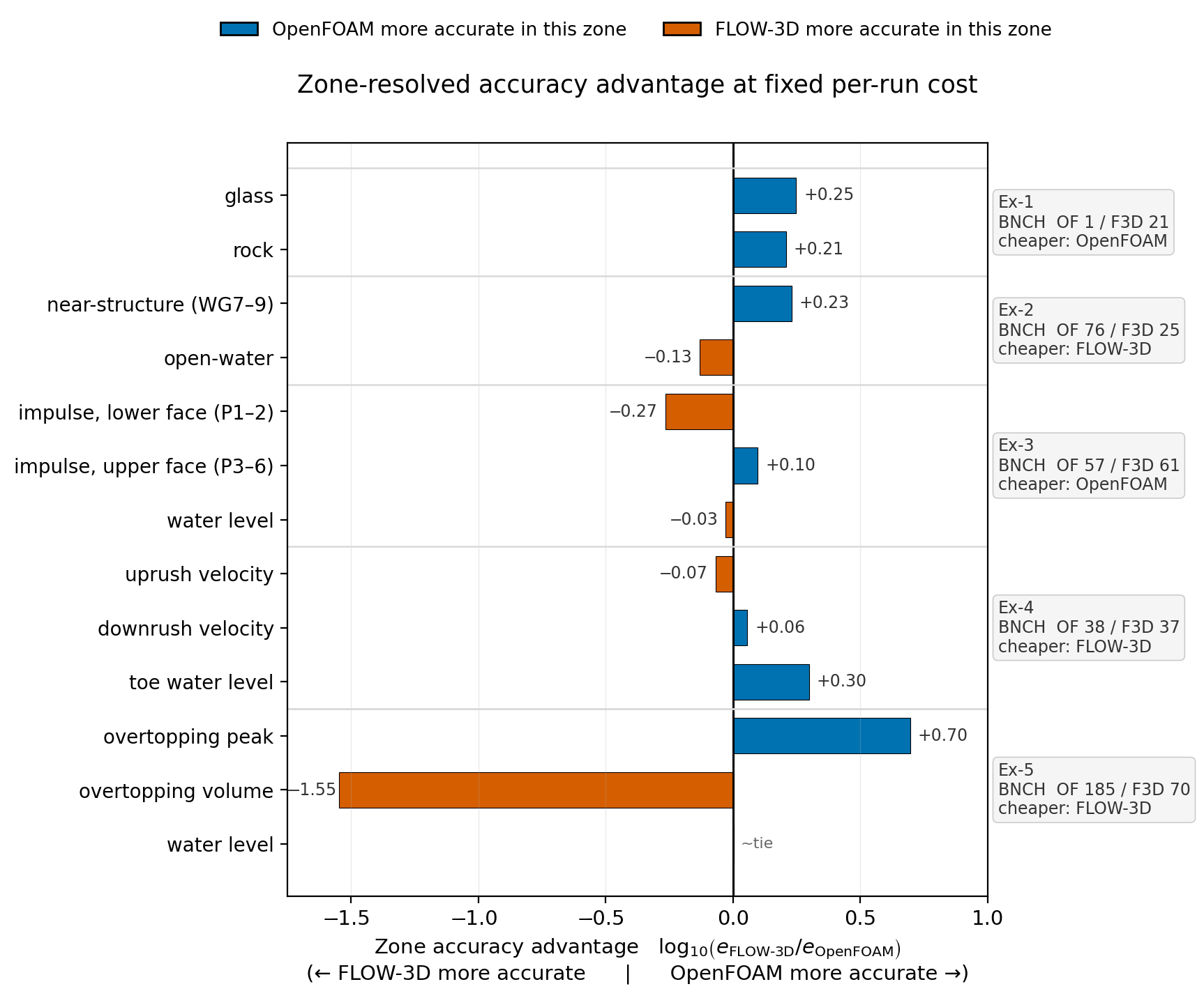
Accuracy and cost are combined here without imposing a preference between them. The cost is a property of a whole run and cannot be attributed to an individual gauge, whereas the accuracy is resolved by location, so the two are first brought together at a fixed per-run cost.

Table 9. Zone-resolved accuracy of the two models at fixed per-run cost. BNCH is identical for all zones of a benchmark.

Benchmark	Zone	e (porousWaveFoam)	e (FLOW-3D)	More Accurate	BNCH (OF/F3D)
Ex-1	glass	0.056	0.099	porousWaveFoam	0.8/11.0
Ex-1	rock	0.028	0.045	porousWaveFoam	0.1/9.8
Ex-2	near-structure (WG7–9)	0.076	0.130	porousWaveFoam	75.9/25.3
Ex-2	open-water	0.079	0.058	FLOW-3D	75.9/25.3
Ex-3	impulse, lower face (P1–2)	0.189	0.103	FLOW-3D	56.9/60.6
Ex-3	impulse, upper face (P3–6)	0.135	0.169	porousWaveFoam	56.9/60.6
Ex-3	water level	0.094	0.088	~ equal	56.9/60.6
Ex-4	uprush velocity	0.661	0.565	FLOW-3D	38.4/37.3
Ex-4	downrush velocity	0.816	0.930	porousWaveFoam	38.4/37.3
Ex-4	toe water level	0.030	0.059	porousWaveFoam	38.4/37.3
Ex-5	overtopping peak	0.023	0.114	porousWaveFoam	184.9/70.0
Ex-5	crest-depth integral	0.310	0.009	FLOW-3D	184.9/70.0
Ex-5	water level	0.220	0.222	~ equal	184.9/70.0

lists the error of each model for every zone of every benchmark alongside the cost of the run that produced it. Within a single benchmark, the more accurate model changes from zone to zone, although the cost does not. In Experiment 2, FLOW-3D is both cheaper and more accurate in open water, while porousWaveFoam is the more accurate near the structure. In Experiment 3, the impulse accuracy reverses between the lower and the upper front face, and in Experiment 5 the overtopping peak favors porousWaveFoam, while the crest-depth integral favors FLOW-3D.

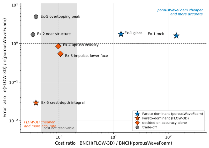
A comparison of the two models on cost and accuracy together, therefore, has to be made for a stated response. Following the work-precision approach standard in numerical-method benchmarking [61], Figure 9 places the governing response of each benchmark on a plane whose axes are the ratio of the two costs and the ratio of the two errors. A model Pareto-dominates the other when it is at least as good on both axes [62], which, on this plane, means that the point falls in the lower-left or upper-right quadrant. The shaded band marks the region within which the cost ratio is smaller than the factor of 2.1 by which the two normalizations of Section 3.3 disagree. A cost difference of that size cannot be separated from the choice of normalization, so the two models are taken as equally expensive there, and the comparison rests on accuracy alone.

Three outcomes follow. The porousWaveFoam is dominant for both porous dam-break media, being 1.6 to 1.8 times more accurate at a cost 14 to 140 times lower. FLOW-3D is dominant for the crest-depth integral of Experiment 5, where it is 34 times more accurate at 0.38 of the cost. The pressure impulse of Experiment 3 and the uprush velocity of Experiment 4 fall inside the cost band, so FLOW-3D is preferable there on accuracy alone. The remaining two responses are genuine trade-offs. FLOW-3D reaches the near-structure water level of Experiment 2 at 0.33 of the cost and the overtopping peak of Experiment 5 at 0.38, but with 1.7 and 5.0 times the error. The choice there depends on what the additional accuracy is worth.

No point falls in a quadrant that would make one model preferable across the set. The two are separated in opposite directions in different benchmarks and, within Experiments 2, 3 and 5, in different zones of the same benchmark at the same cost. Cost-effectiveness is, therefore, not a property of the model but of the pairing between a model and a target response, and Table 9 gives that pairing for each of the fourteen zone-level comparisons made here, with the zone-resolved advantage being shown in Figure 10.

3.5. Why the Responses Are Separated and When a Difference Is Resolvable

The preceding sections report the two models separately for each response, zone and motion phase rather than through one averaged score. The first reason is that no single number represents them. Across the 57 signals for which both models were evaluated, which of the two is the more accurate depends on the metric consulted in 46 cases, or 81%, and in Experiments 3 and 5 at every signal. With nine components, this is what would be expected of two models of comparable overall accuracy, and it is the reason an aggregate score is uninformative here rather than evidence of a systematic dependence in itself. Whether any of these differences is systematic is a separate question, taken up below.

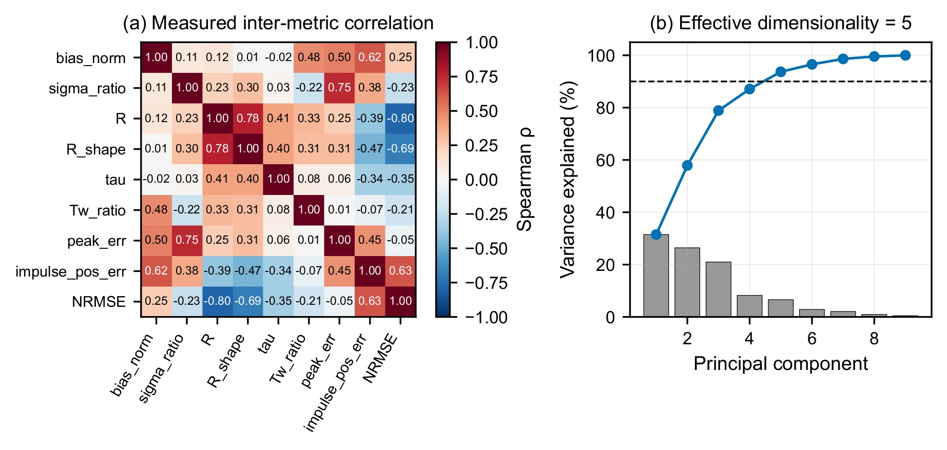
The second is the dimensionality of the metric set. The components are not statistically independent, and the correlation structure was measured rather than assumed. The zero-lag correlation and the normalized RMSE reach a Spearman coefficient of −0.81, the zero-lag and shift-optimized correlations +0.77, and the amplitude ratio and the peak error +0.74. Dependence of this kind does not make the components redundant. Standardizing the metric matrix over the 82 signal–model combinations for which all nine components are defined, five principal components are needed to account for 90% of the variance (Figure 11). The set, therefore, spans five effective dimensions against the one of an aggregate score, so condensing it discards information that no choice of asingle metric recovers.

Averaging can also remove a difference that is present. The pooled bootstrap of Section 3.2.3 returns no distinguishable difference for the twelve gauges of Experiment 2, whereas separating the near-structure gauges from the open-water ones does return one because the two zonal differences carry opposite signs and cancel. Reported as an average, the two models would appear equivalent there for a reason that has nothing to do with their agreement.

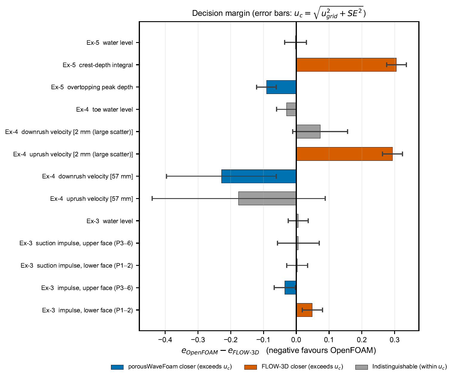
Each difference is, therefore, referred to the combined uncertainty of Section 3.1, whose discretization component is taken as 0.03 from the two grid-convergence assessments of Appendix B. The front position of Experiment 1 lies within 0.7% of its extrapolated value on the grid used, while in Experiment 3 the medium–fine differences have a median of 1.4% and reach 5.6% at the ninetieth percentile. The adopted value, therefore, sits near the upper end of the observed sensitivity. Two comparisons lie close enough to the resulting threshold that a moderately different choice would change them: the upper-face positive impulse at 1.09 times the combined uncertainty and the toe water level of Experiment 4 at 1.00 times.

Table 10. Resolvable differences by benchmark and zone. The difference is the porousWaveFoam error minus the FLOW-3D error, so a negative value favors porousWaveFoam.

Case	Zone	Error Measure	OF	F3D	n	Difference	u_c	Outcome
Ex-3	Impulse, lower face (P1–2)	Positive impulse	0.190	0.141	2	+0.049	0.031	FLOW-3D
Ex-3	Impulse, upper face (P3–6)	Positive impulse	0.135	0.170	4	−0.035	0.032	porousWaveFoam
Ex-3	Suction, lower face (P1–2)	Suction impulse	0.032	0.030	2	+0.003	0.032	Indistinguishable
Ex-3	Suction, upper face (P3–6)	Suction impulse	0.724	0.718	4	+0.006	0.064	Indistinguishable
Ex-3	Water level, all gauges	NRMSE	0.095	0.089	15	+0.006	0.031	Indistinguishable
Ex-4	Uprush velocity, 57 mm	Peak velocity	0.479	0.655	2	−0.176	0.264	Indistinguishable
Ex-4	Downrush velocity, 57 mm	Peak velocity	0.301	0.529	2	−0.228	0.167	porousWaveFoam
Ex-4	Uprush velocity, 2 mm a	Peak velocity	0.846	0.553	2	+0.294	0.031	FLOW-3D
Ex-4	Downrush velocity, 2 mm a	Peak velocity	0.545	0.472	2	+0.073	0.084	Indistinguishable
Ex-4	Toe water level	NRMSE	0.030	0.060	1	−0.030	0.030	Indistinguishable
Ex-5	Overtopping peak depth	Peak error	0.023	0.114	1	−0.091	0.030	porousWaveFoam
Ex-5	Crest-depth integral	Relative error	0.315	0.009	1	+0.306	0.030	FLOW-3D
Ex-5	Water level, all gauges	NRMSE	0.223	0.226	6	−0.003	0.033	Indistinguishable

^a The velocity records at 2 mm from the slope surface carry a much larger measured scatter than those at 57 mm, and no clean flow-reversal instant can be extracted from them; the outcomes for these two entries should be read with that reservation.

applies that test to the governing response of each benchmark and zone, and Figure 12 shows the same comparison graphically. Six of the thirteen comparisons exceed the uncertainty, and seven do not. The largest margin belongs to the crest-depth integral of Experiment 5, at ten times the uncertainty. The reversal of the positive pressure impulse across the front face of Experiment 3 is resolved on both faces, at 1.6 and 1.1 times, with the second of these marginally. At the other end, the free-surface elevation of Experiments 3 and 5 and the toe water level of Experiment 4 differ by no more than the uncertainty itself, and the two models are interchangeable for those responses.

The two elements are, therefore, complementary. Without the decomposition, the ranking would be decided by whichever metric happened to be reported, and a zonal reversal would be averaged away. Without the uncertainty test, more than half of the differences that the decomposition exposes would be taken as real when they are not. Neither element on its own would have produced the separation reported in Table 10.

4. Discussion

4.1. Three Patterns of Difference Between the Two Models

The benchmark results do not reduce to a ranking. Read together, they separate into three patterns, and the distinction between them carries more practical information than any ordering of the two models would.

The first pattern is a difference specific to one model. Its clearest instance is the near-structure phase lag of Experiment 2, where FLOW-3D arrives later than the measurement while porousWaveFoam is synchronized to within the resolution of the record. The decomposition localizes the discrepancy. The shift-optimized shape correlation is essentially identical for the two models in that zone, so the waveform itself is reproduced equally well, and the entire correlation deficit is recovered by a rigid time shift. This excludes numerical diffusion, which would smear the front and degrade the shape correlation, and locates the difference in the propagation speed close to the structure. The lag is confined to that zone. FLOW-3D carries none in open water, and the empty-flume comparison of Section 3.2.1 places the generation-stage difference at 70 ms against the 134 ms measured beside the caisson. A difference of this form is specific to one model. So, for a response that depends on arrival time in the near field, the choice of model matters, and porousWaveFoam is the closer of the two.

The second pattern is a difference that reverses with location or with the design scalar considered. The positive pressure impulse of Experiment 3 changes its leading model between the lower and the upper front face, resolved on the lower face and marginally so on the upper. The overtopping response of Experiment 5 favors porousWaveFoam for the peak crest depth and FLOW-3D for the crest-depth integral, within one and the same event. These reversals cannot be assigned to a single mechanism because the group B differences act simultaneously and none of them was isolated by a dedicated test. What can be said is narrower. A preference established for one response of a structure does not transfer to another response of the same structure, so the target quantity has to be named before a model is chosen.

The third pattern, and the one with the clearest practical implication, is an error shared by both models. The slope velocity of Experiment 4 is damped by both models during uprush and during downrush. The suction impulse of Experiment 3 is lost by both over the upper face, and progressively with height: by 32 to 41% at the fourth transducer and by 78 to 99% at the two above it, with no resolvable difference between the models. The late-time drawdown of Experiment 5 is missed by both. In each case, switching models does not remove the discrepancy, so a better model is not the answer. For the slope velocity, Section 3.2.5 narrows the candidates to what the two models have in common. These are the volume-averaged porous closure and the cell-averaged sampling of a quantity that the experiment measures over a finite volume. For the late-time drawdown of Experiment 5, no such argument is available from the present data. The absence of an absorption layer at the outlet, matched between the two models, is one possible contributor that these experiments cannot separate from other causes.

A further observation concerns the number of quantities the user must supply. The porousWaveFoam configuration carries no turbulence closure, and, therefore, no inlet turbulence quantities, wall functions, wall roughness or near-wall resolution requirement. Dissipation within the porous body is carried by the resistance closure instead (Section 2.1.3). That reduced set of specified inputs does not translate into a systematic loss of accuracy in the responses examined here. For the peak pressure and the water level, the two models differ by amounts that fall within, or only marginally outside, the combined uncertainty of the comparison. This is a practical consideration alongside the accuracy and runtime reported above. These three patterns can be placed against the earlier direct comparisons of the same two models. Bayon et al. [10] for a low Reynolds number hydraulic jump, Fuentes-Pérez et al. [11] for a vertical-slot fishway, and Sabeti et al. [12] for landslide-generated waves all conclude that the two reproduce the measured response satisfactorily. Each reports one response and a small number of aggregate measures. The present results are consistent with that conclusion at the same level of description: averaged over a benchmark, the two models here are also close. What the response-resolved comparison adds is that the conclusion does not extend to the level at which a structure is designed. The ranking changes between responses and between zones of the same structure, and some of the largest errors are shared and, therefore, invisible to any ranking.

4.2. Transfer of the Framework to Irregular Waves

The benchmarks used here are single-event problems: a released water column or an isolated solitary wave and its reflection. Most of the framework transfers to irregular waves unchanged. The normalization by a physical reference, the decomposition into error components, and the test against a combined uncertainty are all defined per signal and do not depend on how many waves the record contains. The between-gauge standard error is simply replaced by the scatter between events.

One definition does have to change. The analysis window, the phase lag and the design scalars are all referred to a primary event identified from the measured record, and under irregular forcing the natural unit becomes the individual wave or the individual overtopping event. The framework would then be applied event by event and the resulting distributions compared, rather than single values. That is the direction indicated by recent overtopping research, in which wave-by-wave rather than mean characteristics govern the risk assessment [31]. Whether the response-dependent reversals reported here persist under such forcing is not established by the present study and would require the corresponding benchmarks to be repeated with irregular waves.

4.3. Limitations

Several limitations bound the conclusions. The comparison is between two configured models rather than two isolated numerical components. The elements listed in group B of Table 1 act simultaneously and cannot be separated by the present design, so no discrepancy reported above is attributed to a single mechanism. The turbulence treatment differs as a user choice (Section 2.1.3). Section 3.2.5 shows that it cannot account for the velocity error the two share, but its effect on each model individually has not been quantified. The correspondence between a response and the part of the model that governs it, raised in Section 1, therefore, remains open: the results establish that the ranking changes from response to response, not which element of the model produces each change.

Each physical phenomenon is represented by a single benchmark model. Only two porous media are compared in the dam-break case, and the ranges of wave height, water depth, porosity and structure geometry are limited. The conditional reversals identified here, therefore, hold within the tested configurations rather than as general properties of either model. Grid convergence was assessed for two of the five benchmarks, chosen to cover the two ways in which the flow is set in motion, so the discretization uncertainty carried into the remaining cases is inferred rather than measured. Two of the comparisons in Table 10 lie close enough to the threshold that their outcome depends on that value.

The computational-cost comparison rests on a single-thread normalization whose limitations are set out in Section 3.3. Differences smaller than the factor of 2.1 by which the two normalization axes disagree are not interpreted on that measure. The reference measurements were digitized from published figures, which constrains the interpretation of absolute error levels (Section 3.1) and sets a floor on the resolution of the timing measures. That floor is reached in Experiment 4, where the scatter of the records taken 2 mm from the slope is large enough that those signals cannot discriminate between the two models at all.

5. Conclusions

FLOW-3D and porousWaveFoam were compared as completely configured models across the five hydraulic benchmarks listed in Table 4. Agreement was decomposed into complementary error components and into the quantities that enter a design check, and each difference was weighed against the uncertainty of the comparison.

Earlier direct comparisons of these two models concluded that both reproduce the measured response satisfactorily, and at the level of a benchmark average, the present results agree. What changes at the level of a design check is that neither model is superior across the responses examined. Their relative accuracy reverses with the porous medium, with position relative to the structure, with the phase of the motion, and with the design quantity chosen for a single response. Five principal components are needed to span 90% of the variance of the metric set, and across 57 signals, the more accurate model changes with the metric consulted in 81% of cases. So, an averaged score cannot represent the comparison.

Several of the largest discrepancies are shared rather than distinguishing. The phase-dependent slope-velocity bias, the suction impulse lost over the upper structure face, and the late-time drawdown in the overtopping case are common to both models, and for these responses, a change of model is not a remedy. Identifying them requires the components to be reported separately, since differences of opposite sign cancel when gauges are pooled.

Of the thirteen governing comparisons, six exceed the combined uncertainty, and seven do not.

Table 11. Summary of response-dependent comparative findings across the five benchmarks.

Experiment	Target Design Response	Conditional Axis	Comparative Outcome
Ex-1	Free-surface profile (amplitude and shape)	Porous-resistance regime	porousWaveFoam leads; margin narrows from glass to rock
Ex-2	Free-surface time series (amplitude, phase)	Spatial zone vs. structure	FLOW-3D better in open water; porousWaveFoam better near the structure
Ex-3	Peak and positive-impulse pressure	Zone across structure face	Both over-predict impulse; leading model reverses across the face, marginally on the upper
Ex-4	Run-up slope velocity	Motion phase (uprush/downrush)	Shared phase-dependent bias, not removed by either model; toe elevation indistinguishable
Ex-5	Peak crest depth vs. crest-depth integral	Design scalar of one response	porousWaveFoam captures the peak depth; FLOW-3D the crest-depth integral

gives the outcome for each response: which model is the closer where the difference is resolved and which responses the two reproduce equally well.

The cost ordering also reverses, but with the size and character of the problem rather than with the response. Per cell, the two are equivalent in the three-dimensional cases without strong local acceleration. The porousWaveFoam is cheaper by one to two orders of magnitude where a two-dimensional representation is admissible and FLOW-3D by about a factor of three where the flow forces a small time step. In wall-clock time, FLOW-3D is faster on all but the smallest problems.

These findings hold within the benchmark configurations tested here rather than as general properties of either model, and the bounds are set out in Section 4.3. The specific rankings are bounded in that way; the procedure that produced them is not. Within that scope, model selection for wave porous structure problems should be governed by the target design response together with a statement of whether the difference exceeds the uncertainty of the comparison, rather than by any single overall ranking. Future work should extend the framework to random-wave conditions, broaden the grid-convergence assessment to the remaining benchmarks, and isolate the contributions of the porous closure and the geometry representation through dedicated single-variable tests.