


Abstract
Leading-edge tubercles provide a bio-inspired modification for regulating the hydrodynamic performance of marine propellers, but their controllable generation on complex three-dimensional blades remains insufficiently studied. This study develops a parametric modeling method for tubercled leading-edge propellers based on the David Taylor Model Basin (DTMB) 4383 geometry. The method combines B-spline smooth reconstruction with a Gaussian envelope function to control tubercle radial peak position and height. After validation with publicly available open-water experimental data, the computational fluid dynamics (CFD) method is applied to uniform and locally targeted tubercled models. The results show that leading-edge tubercles modify the suction-side low-pressure region and redistribute local blade loading. The radial peak position mainly controls the concentration region of the pressure disturbance, whereas peak height affects its intensity. At the design advance coefficient, moving the target peak from r/R = 0.26 to r/R = 0.92 decreased the thrust coefficient by 0.77% and increased the torque coefficient by 1.75%. For a fixed target position, increasing the maximum amplitude ratio from 0.05 to 0.80 increased the thrust and torque coefficients by 0.25% and 0.88%, respectively. These findings indicate that tubercle design should balance radial position and protrusion height.
1. Introduction
As a core component of underwater vehicles and marine propulsion systems, the propeller plays a critical role in determining propulsive efficiency, energy consumption, and overall navigational performance. With the increasing demand for high-efficiency propulsion systems, conventional propellers may suffer from insufficient thrust and efficiency degradation under complex inflow conditions and non-uniform loading. Ebrahimi et al. [1] optimized the hydrodynamic performance of the DTMB 4119 propeller by modifying geometric parameters such as skew angle and chord length distribution, demonstrating that blade geometric reconstruction is an important factor affecting propeller hydrodynamic performance. Therefore, hydrodynamic performance regulation and potential optimization based on novel blade configurations have become an important research direction in the field of naval architecture and ocean engineering.
Bionics provides a new perspective for propeller blade design. Fish and Battle [2] investigated the morphology of humpback whale flippers and suggested that their leading-edge tubercles may contribute to improved flow control capability at high angles of attack. Miklosovic et al. [3] conducted wind-tunnel experiments and found that a humpback whale flipper model with leading-edge tubercles increased the stall angle by approximately 40% and the maximum lift coefficient by approximately 6%. Johari et al. [4] investigated the effects of leading-edge tubercles with different amplitudes and wavelengths on a National Advisory Committee for Aeronautics (NACA) 634-021 airfoil, and reported that a wavy leading edge could improve lift in the post-stall region, with its performance depending on the tubercle amplitude and wavelength.
To clarify the flow-control mechanism of leading-edge tubercles, van Nierop et al. [5] developed a theoretical model and indicated that leading-edge tubercles can alter the local stall characteristics at different spanwise positions, thereby making the overall stall process more gradual. Hansen et al. [6] investigated the performance variations of leading-edge tubercles for different airfoil profiles and found that their effects were related to amplitude, wavelength, and the baseline airfoil geometry. Favier et al. [7] numerically studied an airfoil with a wavy leading edge and reported that the wavy leading edge could modify the flow distribution near the leading edge and affect post-stall performance. Skillen et al. [8] further investigated the flow over a wing with leading-edge undulations and suggested that the wavy leading-edge structure can act as a passive flow-control device in post-stall conditions. Fish et al. [9] reviewed the morphological characteristics, passive flow-control mechanism, and potential applications of humpback whale flipper tubercles in wing-like structures from a bionic perspective, providing a theoretical basis for bio-inspired leading-edge tubercle design.
As the research focus has gradually extended from airfoils to hydrofoils, rudders, and propulsors in marine engineering applications, the hydrodynamic potential of leading-edge tubercles has received increasing attention. Wei et al. [10] experimentally investigated the flow separation control characteristics of hydrofoils with leading-edge tubercles in a water tunnel and found that leading-edge tubercles could modify the stall characteristics and lift-to-drag performance of hydrofoils. Pena et al. [11] conducted a numerical study on a hydrofoil with leading-edge tubercles under turbulent flow conditions and indicated that the effects of leading-edge tubercles on hydrodynamic performance are closely related to the inflow state and operating conditions. Srinivas et al. [12] compared marine rudders with uniform and non-uniform bio-inspired leading-edge tubercles, and found that the non-uniform tubercle distribution could improve post-stall lift and reduce the separated region on the suction side. These studies indicate that leading-edge tubercles have potential for passive flow control in marine lifting surfaces, while their effectiveness is closely associated with geometric parameters and operating conditions.
In recent years, leading-edge tubercles have been introduced into propeller and propulsor design. Butt and Talha [13] numerically investigated the effects of leading-edge tubercles on propeller performance and showed that tubercle parameters could modify the thrust and efficiency characteristics of propellers. Tan et al. [14] investigated the influence of different tubercle amplitudes on the propulsive performance of bio-inspired leading-edge propellers and found that smaller-amplitude configurations exhibited better overall performance than larger-amplitude configurations under certain operating conditions. This indicates that the hydrodynamic effects of leading-edge tubercles are closely related to the amplitude parameter and do not improve monotonically with increasing amplitude. Stark et al. [15] applied leading-edge tubercles to a ducted propeller and analyzed their influence on hydrodynamic performance. Falchi et al. [16] experimentally investigated the effect of leading-edge tubercles on the open-water performance of marine propellers. Asghar et al. [17] applied leading-edge tubercles to propeller blades and analyzed their influence on propulsive performance. Das et al. [18] further experimentally studied the application of wavy leading edges to a ducted controllable-pitch propeller. These studies indicate that leading-edge tubercles can modify the hydrodynamic performance of propellers and propulsors, while their effects are jointly influenced by tubercle amplitude, wavelength, radial distribution, and operating conditions.
With the continued development of bio-inspired propeller research, the controllable generation of leading-edge tubercles on complex three-dimensional propeller blade surfaces has become a key basis for parametric modeling and comparative hydrodynamic performance analysis. Arapakopoulos et al. [19] developed parametric geometric models for marine propellers and indicated that parametric modeling can rapidly generate smooth propeller geometries suitable for numerical analysis while reducing repetitive work in the computer-aided design (CAD) to computer-aided engineering (CAE) conversion process. Pérez-Arribas and Pérez-Fernández [20] proposed a B-spline-based propeller blade design model, in which blade surfaces were generated using geometric parameters with clear hydrodynamic significance, providing a useful reference for the parametric representation of complex free-form blades. Cao and Liu [21] applied cubic B-spline fitting to cylindrical section curves at different radial positions of a marine propeller and further generated the pressure and suction surfaces, demonstrating that radial section curve fitting is an effective approach for constructing three-dimensional propeller blade surfaces. Wang et al. [22] proposed a NURBS-based parametric propeller model, showing that NURBS can effectively describe complex blade surfaces. Zheng et al. [23] developed the iPM4MP model, which describes propeller geometric variations through radial feature curves and provides a reference for automated modeling and design-variable control of complex propeller blades. Njaastad et al. [24] extracted radial blade sections from three-dimensional scanned point clouds and identified geometric parameters such as pitch, skew, chord length, camber, and thickness, further indicating that radial section parameter distributions are essential for describing complex propeller geometry. These studies show that parametric modeling can improve the efficiency of propeller geometry generation and provide a geometric basis for subsequent hydrodynamic performance analysis. However, existing parametric studies on marine propellers mainly focus on conventional geometric parameters such as pitch, chord length, thickness, camber, and skew, whereas further investigation is still required for the refined control of local bio-inspired features such as leading-edge tubercles, particularly their radial distribution and local peak height.
In summary, leading-edge tubercles can influence the hydrodynamic performance of lifting surfaces and propulsors by modifying local pressure distribution and blade loading. However, most existing studies on tubercled propellers have mainly focused on fixed-amplitude, fixed-wavelength, or globally uniform tubercle configurations. For a three-dimensional marine propeller, the local inflow velocity, effective angle of attack, pressure distribution, and blade loading vary significantly along the radial direction because of the combined effects of rotation, twist, chord variation, and skew. Therefore, the hydrodynamic response of a leading-edge tubercle may depend not only on its amplitude and wavelength, but also on where the main tubercle peak is located along the blade span.
The specific unanswered question addressed in this study is how the radial target position and local peak height of leading-edge tubercles affect the pressure redistribution, sectional blade loading, thrust coefficient, torque coefficient, and open-water efficiency of a complex three-dimensional propeller. This question has not been fully resolved by previous studies using globally uniform or fixed-parameter tubercle arrangements, because such configurations cannot independently control the radial concentration position and intensity of the tubercle-induced disturbance. Accordingly, it is necessary to establish a three-dimensional parametric modeling method that can quantitatively control the radial distribution position and peak height of leading-edge tubercles on propeller blades.
Based on the above considerations, this study employs the DTMB 4383 propeller as the baseline geometry and develops a three-dimensional parametric modeling method that integrates the baseline blade geometry with leading-edge tubercle features. The proposed method enables quantitative control of the tubercle peak height and radial target position. To ensure the reliability of the numerical approach, the CFD method is validated using publicly available open-water experimental data and is then applied to the hydrodynamic performance analysis of bio-inspired DTMB 4383 propeller models with leading-edge tubercles. On this basis, different bio-inspired modified models with varying tubercle radial distributions and peak heights are constructed, and their surface pressure distribution, sectional pressure coefficient, thrust coefficient, torque coefficient, and open-water efficiency are comparatively analyzed. This study provides a reference for the parametric modeling and hydrodynamic performance analysis of bio-inspired propellers with controllable leading-edge tubercles.
The remaining sections of this paper are organized as follows. Section 2 introduces the three-dimensional parametric modeling method for the bio-inspired propeller with leading-edge tubercles. Section 3 presents the CFD setup and the validation of the numerical method. Section 4 analyzes the effects of different leading-edge tubercle distributions and peak-height variations on propeller hydrodynamic performance. Section 5 summarizes the main conclusions of this study.
2. Parametric Modeling of Bio-Inspired Propellers with Leading-Edge Tubercles
In studies of bio-inspired propellers with leading-edge tubercles, the continuous and smooth integration of three-dimensional wavy leading-edge features into propeller blade surfaces with twist and variable chord length is fundamental for subsequent hydrodynamic performance analysis. In this section, the DTMB 4383 propeller is adopted as the baseline geometry, and a parametric modeling method for leading-edge tubercles is developed based on B-spline smooth reconstruction and Gaussian envelope control. By controlling the tubercle peak height and target radial position, the proposed method enables quantitative adjustment of the spanwise distribution and local amplitude of the leading-edge tubercles, providing a unified geometric basis for subsequent CFD-based comparative analysis of different bio-inspired configurations.
2.1. Geometric Parameters of the Baseline Propeller for Bio-Inspired Modification
In the parametric modification of bio-inspired propellers, the completeness and accessibility of the baseline propeller geometry directly affect the reliability of model reconstruction and the reproducibility of the results. Therefore, the DTMB 4383 propeller designed by the Naval Ship Research and Development Center (NSRDC) is selected as the baseline propeller for the leading-edge tubercle modification in this study. Boswell [25] systematically investigated the DTMB 4381–4384 series of skewed propellers and provided the main geometric parameters and open-water performance data of this propeller series. The DTMB 4383 propeller is a five-bladed highly skewed propeller with a skew angle of 72°, an expanded area ratio of , a diameter of , and a design advance coefficient of . The DTMB 4383 propeller was selected not only because of the availability of its geometric and experimental data, but also because its highly skewed blade geometry provides a representative and challenging baseline for investigating leading-edge tubercle effects on complex marine propellers. Compared with conventional or lower-skewed propellers, the DTMB 4383 propeller has a more pronounced radial skew distribution and a stronger three-dimensional blade shape. These geometric characteristics lead to more evident radial variations in local blade loading, inflow angle, and pressure distribution. Moreover, its highly skewed and curved leading-edge geometry provides a suitable geometric basis for introducing bio-inspired tubercle features, since the humpback whale flipper, from which the leading-edge tubercle concept is inspired, is also characterized by a curved leading edge with spanwise morphological variation. Therefore, the DTMB 4383 propeller is suitable for examining whether the proposed parametric modeling method can smoothly integrate leading-edge tubercles into a complex propeller geometry and for investigating how the radial position and peak height of tubercles affect the hydrodynamic performance. In this sense, the DTMB 4383 propeller provides a more demanding test case for studying the radial distribution effects of leading-edge tubercles than a simpler low-skewed baseline propeller.
The sectional geometric parameters of the DTMB 4383 propeller listed in Table 1 are obtained from the publicly available data compiled by Bal [26]. is the radial position of the current section, is the propeller radius, is the sectional chord length, is the propeller diameter, is the pitch, is the maximum sectional thickness, and is the maximum sectional camber. Accordingly, , , , , , and denote the non-dimensional radial position, chord-to-diameter ratio, pitch-to-diameter ratio, rake-to-diameter ratio, maximum-thickness-to-diameter ratio, and maximum-camber-to-chord ratio, respectively. In this study, the DTMB 4383 geometry is defined by both the main propeller parameters and the radial sectional parameters. According to the standard geometric description of marine propellers [27], a propeller blade can be represented by a series of radial sections distributed from the root to the tip. Each radial section is defined by its radial position, chord length, pitch, skew, rake, thickness distribution, and camber distribution. The main propeller parameters describe the overall propeller configuration, while the sectional parameters in Table 1 describe the radial distributions of chord length, pitch, skew, rake, maximum thickness, and maximum camber. Therefore, these data provide the complete geometric input required for the subsequent three-dimensional reconstruction of the baseline propeller.
Table 1.
Sectional geometric parameters of the DTMB 4383 propeller.
In the reconstruction process, the non-dimensional radial position was first used to locate each blade section along the spanwise direction. The chord-to-diameter ratio , maximum-thickness-to-diameter ratio , and maximum-camber-to-chord ratio were used to define the size and sectional shape characteristics of each radial profile. The pitch-to-diameter ratio was used to determine the local pitch setting of the section, while the skew angle and rake-to-diameter ratio were used to determine the circumferential and axial offsets of the section, respectively. Through this procedure, the two-dimensional sectional profiles were transformed into the three-dimensional cylindrical coordinate system of the propeller and then used for blade-surface reconstruction.
Based on the geometric definition given by the main propeller parameters and the sectional data in Table 1, the DTMB 4383 baseline propeller was reconstructed through a combined MATLAB and Siemens NX modeling procedure. In this procedure, MATLAB R2022a was used for parameter processing, radial section calculation, matrix operation, and coordinate transformation from the two-dimensional sectional coordinate system to the three-dimensional cylindrical coordinate system of the propeller. This is beneficial for the automatic generation of multiple radial section profiles and for maintaining consistency in the geometric reconstruction process.
The generated section data were then imported into Siemens NX 2412 using a Python 3.9-based automation script. Siemens NX was used for spatial curve fitting, blade surface lofting, surface stitching, solid generation, and circumferential blade patterning. Therefore, the combination of MATLAB and Siemens NX takes advantage of MATLAB in numerical calculation and parametric data processing, while using Siemens NX for robust three-dimensional surface reconstruction and solid modeling. This combined workflow reduces manual modeling operations, improves the repeatability of model generation, and provides a consistent geometric basis for subsequent bio-inspired modification and CFD analysis. The reconstructed three-dimensional baseline propeller model is shown in Figure 1.
Figure 1.
Three-dimensional model of the DTMB 4383 baseline propeller.
To ensure the controllability of geometric variables before and after introducing the bio-inspired features, the pitch distribution, skew distribution, rake distribution, thickness distribution, and basic sectional characteristics of the baseline propeller are kept unchanged in the subsequent modification process. Only the local chord length and leading-edge profile in the leading-edge region are nonlinearly reconstructed. This treatment ensures that the geometric differences among different bio-inspired models mainly originate from the distribution pattern and peak height of the leading-edge tubercles, thereby providing a consistent geometric basis for the subsequent comparative analysis of hydrodynamic performance.
2.2. Parametric Generation and Control of Leading-Edge Tubercles
To achieve continuous and quantitative control of the protrusion height, spanwise distribution density, and local target position of the wavy leading edge, a three-dimensional targeted parametric modeling program was developed in this study. The superposition of the wavy leading edge onto the baseline propeller is not implemented by simply stretching the original three-dimensional geometry; instead, it is achieved through Gaussian-envelope mapping of discrete feature control points and B-spline-based reconstruction of the underlying profile data. The detailed generation and control procedure is as follows:
2.2.1. Radial Section Interpolation and Waveform Control-Point Generation
Since the original geometric parameters of the DTMB 4383 baseline propeller are only provided at a limited number of radial sections, it is difficult to directly describe the continuous geometric variation in the wavy leading edge along the spanwise direction. To improve the geometric reconstruction accuracy of the leading-edge tubercle distribution, linear interpolation is first performed on the geometric parameters between adjacent original radial sections. Specifically, equally spaced interpolated sections are inserted between any two adjacent original sections while retaining the original section data. The total number of refined radial sections is given by
where is the number of original radial sections, and is the number of interpolated sections inserted between two adjacent original sections. In this study, and ; therefore, . The value was selected based on preliminary geometric tests and reconstruction checks for the present propeller model. It was adopted as a compromise between geometric resolution and modeling efficiency. With this setting, the original 11 radial sections are refined into 211 sections, which provides sufficient spanwise resolution to represent the Gaussian-envelope-controlled amplitude distribution and the B-spline reconstructed wavy leading edge. In the generated geometry, the tubercle peak and valley regions can be smoothly described without visible discontinuities, as shown in Figure 2. Further increasing would produce more radial sections and a denser point cloud, but would also increase the workload of surface reconstruction and subsequent mesh generation. Therefore, was adopted in this study to ensure a smooth geometric representation while maintaining reasonable modeling efficiency.
Figure 2.
Interpolated radial section curves near the leading-edge tubercle peak region.
The refined radial sections provide a high-density geometric basis for the continuous spanwise distribution of the leading-edge tubercles and the subsequent three-dimensional surface reconstruction. Figure 2 shows the detailed interpolated section curves near the tubercle peak region.
To facilitate the description of the distribution pattern of the wavy leading edge along the blade span, the non-dimensional radial position is defined as
where is the actual radial position and is the propeller radius. The wavelength-to-span ratio is then introduced as a control parameter for the spanwise distribution density of the wavy leading edge, where is the effective spanwise range and is the target wavelength. To reduce the interference of wavelength variation on the hydrodynamic performance comparison, the same wavelength-to-span ratio is used for all bio-inspired models in this study, namely . The number of wave periods is automatically determined according to the target wavelength as follows:
Based on , the alternating wave peak and valley control points are further generated. The number of control points is given as follows:
Under the present setting, , and the rounded number of wave periods is . The integer wave number is adopted to ensure that the leading-edge tubercle distribution consists of complete peak–valley periods along the effective blade span. This treatment avoids incomplete wave segments near the root or tip region, which may introduce additional end effects and make the comparison among different target positions less consistent. Although the rounding operation would lead to a stepwise change in if were varied continuously, is not used as a design variable in the present study. Instead, all bio-inspired models use the same , so the wavy leading-edge distribution density remains consistent among different cases. Therefore, the subsequent comparisons mainly reflect the effects of wave peak position and wave height variation rather than changes in wavelength density. Accordingly, alternating wave peak/valley control points are generated. This setting ensures that different bio-inspired models have a consistent wavy leading-edge distribution density, so that the subsequent comparisons mainly reflect the effects of wave peak position and wave height variation.
2.2.2. Phase Locking and Gaussian-Envelope Amplitude Mapping
To achieve quantitative control of the local position of leading-edge tubercles, a phase-locking mechanism is introduced during the generation of wave peak and valley control points. Specifically, the program first searches the spanwise control-point sequence for the control point closest to the prescribed target position. This control point is then reset to the target radial position and forced to act as a wave peak. Through this treatment, the local enhancement center can always coincide with a wave-peak control point regardless of the variation in target position, thereby enabling controllable movement of the local leading-edge tubercle enhancement.
After the sequence of wave peak and valley control points is obtained, a Gaussian envelope function is used to map the protrusion height of the wave peaks. For the -th wave-peak control point, its non-dimensional radial position is denoted as , and the corresponding absolute protrusion height is defined as
where is the actual chord length of the radial section at the -th wave-peak control point, is the baseline amplitude ratio, is the maximum amplitude ratio at the target center, is the non-dimensional radial position of the target enhancement center, and is the influence-range coefficient of the Gaussian envelope. For the wave-valley control points, so that the valleys remain on the original leading-edge curve of the baseline propeller.
Based on the above Gaussian-envelope control equation, the wavy leading-edge models in this study are divided into two categories: uniform spanwise wavy models and locally targeted wavy models. For the uniform spanwise wavy model, the amplitude ratios are set as
In this case, all wave peaks have the same relative protrusion height, and the absolute peak height varies only with the local chord length:
This model represents a uniformly distributed leading-edge tubercle configuration along the blade span. The geometric parameters of the leading-edge tubercles are defined in Figure 3.
Figure 3.
Definition of the geometric parameters of leading-edge tubercles.
For the locally targeted wavy model,
where represents the baseline amplitude ratio away from the target center, and represents the maximum amplitude ratio at the target center. In this study, the locally targeted models use , , and , while only the target center position and the maximum amplitude ratio are varied. The value was selected based on preliminary geometric tests and reconstruction checks for the present propeller model. In the Gaussian envelope, controls the radial influence range of the local tubercle-height enhancement. When the distance from the target center is equal to , the additional amplitude term decreases to approximately 60.7% of its peak value; when the distance reaches , it decreases to approximately 13.5%. Therefore, confines the main enhancement within a local radial region around the prescribed target position, while still maintaining a smooth transition to the baseline amplitude away from the target center. This setting avoids an excessively narrow protrusion-height concentration, which may introduce abrupt geometric variations, and also avoids an overly broad distribution, which would make the targeted model close to a globally distributed tubercle configuration.
As shown in Figure 4, the Gaussian envelope defines the radial distribution of the tubercle protrusion height, while the B-spline reconstructed waveform provides a smooth spanwise variation in the wavy leading edge. In this example, indicates that the target wave peak is located at the radial position of , while indicates that the maximum protrusion height at the target center is 80% of the local chord length. The black triangular markers represent the alternating peak and valley control points used for waveform construction. The valley points remain on the baseline leading edge, where the protrusion height is zero, whereas the peak points are assigned different amplitudes according to the Gaussian envelope. Therefore, the protrusion height reaches its maximum near the target radial position and gradually decreases away from the target center.
Figure 4.
Gaussian-envelope-controlled radial distribution of tubercle amplitude and B-spline reconstructed waveform.
The B-spline curve connects these discrete control points smoothly and avoids abrupt geometric changes along the radial direction. The three-dimensional propeller model inserted in the upper-right corner of Figure 4 further illustrates how the radial amplitude distribution is reflected in the actual leading-edge geometry of the blade. This figure demonstrates that the proposed method can transform the complex wavy leading-edge geometry into two controllable design variables, namely the wave-peak position and wave-peak height, which provides a clear geometric basis for the subsequent hydrodynamic performance comparisons.
2.2.3. B-Spline Smooth Reconstruction and Chordwise Disturbance Attenuation
After obtaining the discrete height control points of wave peaks and valleys, directly connecting these points with linear segments may introduce geometric corners between adjacent control points, which can reduce the smoothness of subsequent surface reconstruction. Therefore, the discrete height points are used as interpolation data points, and an order-4 B-spline interpolation method is adopted to smoothly reconstruct the spanwise protrusion-height distribution. In this way, a continuous leading-edge protrusion-height function is obtained. According to the standard B-spline formulation [28,29], the B-spline curve can be expressed as
where denotes the control points obtained during the B-spline interpolation process, rather than the original wave peak/valley interpolation data points; is the order of the B-spline, which is set to in this study; and is the -th order B-spline basis function. The B-spline basis functions are evaluated using the Cox–de Boor recursion formula [28,29], which is given by
Through order-4 B-spline interpolation, a continuous leading-edge protrusion-height distribution is obtained. The order-4 B-spline corresponds to a cubic B-spline and has continuity at internal simple knots, meaning that both the first and second derivatives are continuous. This property helps reduce curvature discontinuities in the protrusion-height distribution, thereby decreasing the risk of abnormal pressure gradients and numerical oscillations caused by geometric discontinuities. After the B-spline reconstruction, the generated leading-edge curves and three-dimensional blade surfaces were further checked. The reconstructed leading-edge tubercle curves were inspected to ensure smooth peak–valley transitions, and the lofted blade surfaces were checked to avoid local self-intersections, abrupt geometric corners, and obvious local concavities near the leading-edge region. Within the parameter range considered in this study, the reconstructed tubercled leading edges maintained smooth geometric continuity and did not show unintended local concave regions that could act as artificial flow-separation triggers. Therefore, the hydrodynamic differences among different models are mainly attributed to the prescribed tubercle distribution and peak height, rather than to abnormal geometric defects introduced during surface reconstruction.
To avoid rigidly stretching the entire blade section due to the leading-edge tubercles, a chordwise disturbance attenuation function is further introduced. This function allows the leading-edge protrusion to gradually decay from the leading edge to the trailing edge. For the -th radial section, the equivalent chord length at the leading edge after adding the protrusion is defined as
For the -th chordwise node on this section, the local equivalent chord length is defined as
where is the original chord length of the -th radial section of the baseline propeller, is the equivalent chord length at the leading edge after adding the protrusion, is the normalized chordwise coordinate of the -th node from the leading edge to the trailing edge, and is the total number of chordwise nodes. When , the node corresponds to the leading edge, where the leading-edge tubercle disturbance reaches its maximum. When , the node corresponds to the trailing edge, where the local equivalent chord length recovers to the original chord length of the baseline propeller. This treatment allows the leading-edge tubercle disturbance to attenuate gradually along the chordwise direction, avoiding rigid stretching of the entire section while maintaining the stability of the trailing-edge position and sectional topology. The linear attenuation in Equation (13) is adopted as a first-order geometric treatment rather than a strict fluid-dynamic law. Its purpose is to localize the geometric modification near the leading edge, where the tubercle is introduced, and to smoothly recover the original blade section toward the trailing edge. This is consistent with the physical role of leading-edge tubercles as a leading-edge flow-control feature, because the geometric perturbation and the associated pressure disturbance are expected to be strongest near the leading-edge region and gradually weaken downstream along the chord.
Alternative chordwise attenuation functions, such as cosine, exponential, or higher-order polynomial decay functions, could modify the detailed chordwise distribution of the geometric perturbation and may therefore affect the local pressure coefficient distribution, especially in the mid-chord region. However, in the present study, the same linear attenuation function is used for all bio-inspired models. Therefore, the comparative results mainly reflect the effects of radial target position and peak height, rather than differences caused by the chordwise attenuation form. The influence of different chordwise attenuation functions will be further investigated in future work.
2.2.4. Local Leading-Edge Point Refinement and Three-Dimensional Solid Generation
Considering the large curvature variation in the leading-edge tubercle region, nonlinear local refinement is applied to the point-cloud distribution near the airfoil leading edge. The chordwise refinement mapping function is defined as
where is the reference length of the refined region, is the density control factor, and is a uniformly distributed parametric variable. In this study, . This mapping is mainly applied to the local leading-edge region satisfying , while the conventional chordwise point distribution is retained for the mid- and aft-chord region where . This point-distribution strategy improves the point-cloud resolution in the leading-edge tubercle region and provides a smoother geometric input for subsequent CFD mesh generation and hydrodynamic performance calculation.
The two-dimensional NACA thickness and camber data with the superimposed wavy protrusions are then combined with the pitch angle, skew angle, and rake angle of each baseline blade section. Through spatial coordinate transformation matrices, these section data are mapped into a three-dimensional cylindrical coordinate system to generate the three-dimensional point-cloud coordinates of the upper and lower blade surfaces at each radial section. The generated coordinates are then exported as data exchange files for subsequent automated modeling.
Finally, secondary development is performed using the Siemens NX 2412 Open API with Python 3.9. The developed script automatically reads all interpolation-point files and sequentially executes section-curve fitting, surface lofting, upper- and lower-surface stitching, solid hub generation, and circumferential blade patterning. In this way, the manual modeling process is converted into an automated modeling workflow, which helps reduce human modeling errors and improve the consistency of model construction.
2.3. Parametric Model Matrix and Selection of Representative Models
Based on the above parametric generation method for leading-edge tubercles, a set of bio-inspired modified propeller models was established based on the DTMB 4383 propeller. According to the geometric characteristics of the leading-edge tubercles, the modified models were divided into two categories: uniform tubercled leading-edge models and locally targeted tubercled leading-edge models.
For the uniform tubercled leading-edge models, the tubercle amplitude was kept constant along the radial direction, namely . Three uniform-amplitude models were constructed, corresponding to , 0.35, and 0.80.
For the locally targeted tubercled leading-edge models, the target center position and the maximum amplitude ratio were used as the main control parameters. Two groups of parametric models were established. In the first group, was kept constant, while was varied as 0.26, 0.37, 0.48, 0.59, 0.70, 0.81, and 0.92, resulting in seven models. In the second group, was kept constant, while was varied as 0.05, 0.20, 0.35, 0.50, 0.65, and 0.80, resulting in six models. For the locally targeted models, except for and , the remaining parameters were kept unchanged to ensure comparability among different models, namely , , and .
Considering both the uniform and locally targeted tubercled leading-edge models, the locally targeted model with overlaps geometrically with the uniform small-amplitude model . In addition, the two groups of locally targeted models share an identical geometry at and . Therefore, 14 different bio-inspired modified geometries with leading-edge tubercles were finally established. Including the DTMB 4383 baseline propeller, the complete model set contains 15 geometric models, as listed in Table 2.
Table 2.
Complete model matrix of the baseline and leading-edge tubercled propeller models.
To illustrate the geometric differences among different types of leading-edge tubercle models, six representative models were selected from the complete model set for geometric comparison, including the DTMB 4383 baseline propeller, the uniform small-amplitude model , the uniform medium-amplitude model , and three locally targeted models , , and , as shown in Figure 5.
Figure 5.
Geometric comparison of representative propeller models selected from the complete model matrix: (a) M0; (b) M1; (c) M2; (d) M7; (e) M14; (f) M9. M0 is the DTMB 4383 baseline propeller; M1 and M2 are uniform tubercled leading-edge models; M7, M14, and M9 are targeted tubercled leading-edge models. The complete model matrix is listed in Table 2.
In summary, a parametric modeling procedure capable of controlling the position and amplitude of leading-edge tubercles was established based on the Gaussian envelope function and B-spline smooth reconstruction. By adjusting the target position and the maximum amplitude ratio , bio-inspired propeller models with different tubercle distributions and protrusion heights can be generated. Figure 5 only presents representative geometric features of different types of leading-edge tubercle models, while the complete model set is defined by the model matrix listed in Table 2.
3. Numerical Method and Validation
To ensure the reliability of the hydrodynamic performance analysis of the subsequent DTMB 4383 bio-inspired propeller models with leading-edge tubercles, a unified CFD numerical method is first established in this study. The numerical method includes solver settings, turbulence model selection, computational domain definition, boundary condition specification, mesh generation strategy, and near-wall treatment. On this basis, a propeller with publicly available open-water experimental data is selected as the validation case to verify the reliability of the numerical method. After validation, the same computational method is applied to the comparative hydrodynamic performance analysis of different DTMB 4383 bio-inspired propeller models with leading-edge tubercles.
3.1. Numerical Model and Hydrodynamic Coefficients
A pressure-based steady solver is adopted to simulate the open-water performance of the propeller. The Multiple Reference Frame (MRF) method is used to account for the rotational effect of the propeller. In the MRF approach, an angular velocity consistent with the propeller rotation is assigned to the rotating domain, thereby transforming the rotating flow problem into a steady-state calculation. This treatment enables the main hydrodynamic performance parameters of the propeller to be obtained with reasonable computational efficiency. It should be noted that the MRF method provides a steady, time-averaged representation of the rotating flow field and does not explicitly resolve transient flow structures such as vortex shedding or time-dependent pressure fluctuations. In the present study, the main objective is to compare the mean open-water performance of different bio-inspired propeller geometries, including the thrust coefficient, torque coefficient, and open-water efficiency, under the same numerical framework. Therefore, the MRF approach is considered appropriate for evaluating the relative influence of leading-edge tubercle position and height on the mean hydrodynamic performance. However, leading-edge tubercles may introduce local unsteady vortical structures near the blade leading edge and tip region. These unsteady effects may influence instantaneous pressure fluctuations, local vortex dynamics, and noise-related characteristics, which cannot be fully captured by the present steady MRF simulation. Therefore, the efficiency conclusions in this study should be interpreted as steady-state, time-averaged open-water performance trends. A more detailed investigation of unsteady flow mechanisms using transient simulations, such as sliding-mesh unsteady Reynolds-averaged Navier–Stokes (URANS) simulations or large eddy simulation (LES), will be considered in future work.
From the perspective of propeller hydrodynamics, the open-water performance of a marine propeller is governed by the thrust and torque generated by the pressure and viscous shear forces acting on the blade surfaces. The thrust represents the useful axial force produced by the propeller, whereas the torque represents the rotational moment required to drive the propeller. Therefore, the propulsive efficiency depends on the balance between useful thrust generation and torque consumption. For a propeller operating under open-water conditions, the local circumferential velocity increases with the radial position. As a result, geometric modifications located in the outer radial region may have a stronger influence on the overall torque and efficiency. In the present study, the leading-edge tubercles modify the local leading-edge geometry and then affect the blade-surface pressure distribution and sectional loading. These local hydrodynamic changes are finally reflected in the overall thrust coefficient, torque coefficient, and open-water efficiency.
Based on this hydrodynamic understanding, thrust, torque, and efficiency are used as the main indicators for evaluating propeller propulsion performance [30]. In open-water performance evaluation, non-dimensional parameters are commonly used. According to propeller hydrodynamic theory, the advance coefficient , thrust coefficient , torque coefficient , and open-water efficiency are defined as follows:
where is the propeller advance velocity, in m/s; is the propeller rotational speed, in r/s; is the propeller diameter, in m; is the density of water, taken as ; is the thrust generated by the propeller, in N; and is the propeller torque, in N·m.
Considering that the boundary-layer state near the blade surface can affect the prediction of thrust and torque coefficients, the Transition Shear Stress Transport (SST) model is employed in this study. This model is based on the SST k-ω turbulence model proposed by Menter [31] and incorporates the γ-Reθ transition model developed by Menter et al. [32] and Langtry and Menter [33]. Two additional transport equations, namely the intermittency factor γ and the transition momentum-thickness Reynolds number Reθt, are introduced to describe natural transition, bypass transition, and separation-induced transition. Compared with fully turbulent models, the Transition SST model can account for the variation in laminar, transitional, and turbulent regions on the blade surface to a certain extent. Therefore, it is more suitable for the near-wall flow simulation of bio-inspired propellers with leading-edge tubercles in this study.
To further support the selection of the turbulence model, an additional turbulence-model sensitivity analysis was conducted for the DTMB 4381 validation case at the design advance coefficient . Three turbulence models were compared, namely the Transition SST model, the fully turbulent SST - model, and the Standard - model. The calculated open-water performance coefficients and their relative errors are listed in Table 3.
Table 3.
Turbulence-model sensitivity analysis for the DTMB 4381 validation case at .
As shown in Table 3, the Transition SST model provides the best overall agreement with the experimental data. The errors of , , and are 2.14%, 2.86%, and 0.74%, respectively. In comparison, the SST - model and the Standard - model show larger deviations in and , although their errors in 10 are relatively small. Therefore, the Transition SST model was adopted in the subsequent simulations to maintain better overall prediction accuracy for thrust, torque, and open-water efficiency, as well as consistency in the comparison of different tubercled propeller models.
3.2. Computational Domain and Boundary Conditions
3.2.1. Computational Domain
To simulate the operating condition of the propeller in open water, a typical cylindrical computational domain was constructed. The computational domain was divided into an inner rotating domain enclosing the propeller and an outer stationary domain used to represent the far-field flow.
The specific dimensions of the computational domain were defined as follows. The diameter of the rotating domain was set to 1.2D, where D is the propeller diameter. The inlet boundary of the stationary domain was located 4D upstream of the propeller disk plane, while the outlet boundary was located 10D downstream. The diameter of the outer cylindrical domain was set to 6D. Flow variables were transferred between the rotating and stationary domains through an interface. To illustrate the computational-domain arrangement adopted in this study, Figure 6 presents the domain configuration using the DTMB 4381 validation case as an example. The same domain dimensions, boundary conditions, and rotating-domain settings were applied to the subsequent DTMB 4383 bio-inspired propeller models with leading-edge tubercles.
Figure 6.
Computational domain configuration for the DTMB 4381 validation case. The same computational-domain arrangement was applied to the DTMB 4383 bio-inspired propeller models.
3.2.2. Boundary Conditions and Operating Conditions
The inlet boundary was defined as a velocity inlet, and the outlet boundary was defined as a pressure outlet with a gauge pressure of 0 Pa. The outer cylindrical surface was set as a slip wall. The blade and hub surfaces were treated as no-slip walls. In the rotating domain, an angular velocity was assigned through the rotating reference frame to simulate the rotational motion of the propeller. The interface between the rotating and stationary domains was used to transfer flow-field variables.
During the simulations, the propeller rotational speed was kept constant at . According to the definition of the advance coefficient, different operating conditions were achieved by adjusting the inlet velocity . In this study, , 0.5, 0.7, 0.889, and 1.0 were selected as the main operating conditions for the subsequent DTMB 4383 bio-inspired propeller models with leading-edge tubercles, where corresponds to the design condition.
3.3. Mesh Generation and Near-Wall Treatment
Mesh quality directly affects the accuracy and convergence of numerical simulations of propeller flow fields. In this study, the flow domain was discretized using an unstructured hybrid mesh in ANSYS Fluent 2024 R2 Meshing. The closed rotating and stationary fluid domains were meshed through surface mesh generation, boundary-zone identification, volume mesh generation, and prism-layer generation. This meshing strategy improves the adaptability of the mesh to complex bio-inspired geometries such as leading-edge tubercles. According to the flow characteristics of propellers under open-water conditions, the computational domain was divided into an inner rotating domain enclosing the propeller and an outer stationary domain. Flow variables and fluxes were transferred between the two domains through an interface.
The mesh size was set according to the principle of refinement near the propeller and gradual coarsening in the far-field region. In the rotating domain, local mesh refinement was applied to the blade surface, hub, blade tip, leading edge, and trailing edge, where relatively large geometric curvature and flow gradients occur. In the outer stationary domain, which is far from the propeller and has relatively small flow variations, a larger volume mesh size was adopted to reduce the computational cost. The same mesh size was maintained on both sides of the interface between the rotating and stationary domains to reduce interpolation errors of flow variables. During surface mesh generation, the Curvature & Proximity size function was enabled to enhance the resolution of regions with large curvature variations. For local regions with evident geometric changes, such as the leading-edge tubercles, trailing edge, and blade-tip edges, local edge refinement was applied to ensure sufficient resolution of the bio-inspired leading-edge geometry. In particular, for the DTMB 4383 bio-inspired propeller models, edge refinement was imposed along the wavy leading-edge tubercle curves, so that the peak and valley regions of the tubercles could be resolved more smoothly during surface mesh generation.
The volume mesh was generated using the Poly-Hexcore method in Fluent Meshing. This method uses polyhedral cells near complex wall surfaces to adapt to the curved propeller geometry, while generating hexahedral-dominant cells in the core region away from the wall, thereby balancing geometric adaptability and computational efficiency. The minimum and maximum volume mesh sizes in the rotating domain were 0.3 mm and 4.8 mm, respectively. For the outer stationary domain, the minimum and maximum volume mesh sizes were 2 mm and 32 mm, respectively.
After mesh generation, the mesh quality was further evaluated using surface skewness and orthogonal quality. The surface skewness was used to assess the quality of the surface mesh, while the orthogonal quality was used to evaluate the volume mesh. The mesh quality statistics of the DTMB 4381 validation model are listed in Table 4. For the rotating domain, the surface mesh contained 195,568 faces, among which only 39 faces had a skewness larger than 0.50. The average and maximum surface skewness values were 0.0316 and 0.7196, respectively. For the outer stationary domain, the surface mesh contained 121,338 faces, and only 2 faces had a skewness larger than 0.50. The average and maximum surface skewness values were 0.0166 and 0.5133, respectively.
Table 4.
Mesh quality statistics of the DTMB 4381 validation model.
For the volume mesh, the rotating domain contained 1,979,209 cells, and the outer stationary domain contained 716,698 cells. No cells with an orthogonal quality lower than 0.2 were observed in either domain. The minimum orthogonal quality values of the rotating and outer stationary domains were 0.2001 and 0.3129, respectively. These results indicate that the generated mesh satisfies the adopted mesh-quality criteria and is suitable for the present open-water propeller simulations.
To account for the influence of the near-wall boundary layer on the flow-field calculation, prism-layer meshes were generated near the propeller blades and hub. The boundary layer in the rotating domain consisted of 12 layers, with a growth rate of 1.2 and a first-layer height of 0.05 mm. The boundary layer in the outer stationary domain consisted of 8 layers, with a growth rate of 1.2 and a first-layer height of 1 mm.
Figure 7 shows the mesh generation strategy using the DTMB 4381 validation model as an example. For the subsequent DTMB 4383 bio-inspired propeller models with leading-edge tubercles, the same computational domain size, mesh topology, and mesh-size control principles were adopted, with additional local refinement applied to regions with geometric variations, such as the leading-edge tubercles, blade tip, and blade edges. After applying the above mesh generation method to the DTMB 4381 validation model, the rotating domain contained approximately cells, the outer stationary domain contained approximately cells, and the total mesh number was approximately .
Figure 7.
Mesh details of the DTMB 4381 validation case. The same mesh generation strategy was applied to the DTMB 4383 bio-inspired propeller models.
According to the distribution, most regions of the blade surface had values in the range of 3–8, while relatively higher values appeared only near the leading edge, blade tip, and local edge regions, with a maximum value of approximately 15. This result indicates that the present boundary-layer mesh can adequately resolve the near-wall flow around the blade. Since the Transition SST model used in this study has relatively high requirements for near-wall mesh resolution, the current boundary-layer mesh setting is considered suitable for the open-water performance prediction of the propeller. It should be noted that the relatively higher y+ values appear only in limited high-curvature regions and do not represent the overall near-wall resolution of the blade surface. For the leading-edge tubercle region, the local edge refinement and prism-layer mesh were used together to reduce the possible influence of high curvature on the near-wall resolution. Therefore, the present mesh is considered adequate for predicting the overall open-water performance and for comparing the relative trends of local pressure distribution and sectional loading among different bio-inspired models. Nevertheless, the local pressure prediction near the leading-edge tubercles may still be affected to some extent by the near-wall mesh resolution because of the strong local curvature and pressure gradient in this region. For this reason, the sectional pressure-distribution results in this study are mainly used to analyze comparative trends in pressure redistribution and sectional loading under the same mesh-generation strategy, rather than to provide a fully mesh-independent description of very small-scale local flow structures. Since all bio-inspired propeller models were generated and meshed using the same refinement principles, the relative comparison among different radial target positions and peak-height settings remains consistent.
Overall, local refinement was applied near the blade surface, blade tip, blade edges, hub, and rotating–stationary interface, while larger mesh sizes were used in the far-field region away from the propeller. The mesh quality statistics, together with the near-wall y+ distribution, indicate that the present mesh can provide a reasonable balance between computational accuracy and computational cost.
3.4. Numerical Validation Based on DTMB 4381 Open-Water Performance
3.4.1. Validation Model and Experimental Data Source
The DTMB 4381 propeller and the DTMB 4383 baseline propeller used in this study both belong to the DTMB 4381–4384 series of model propellers. They have the same blade number, diameter, expanded area ratio, design advance coefficient, and basic sectional parameter framework, while the main geometric difference lies in the skew distribution [25]. Therefore, the DTMB 4381 propeller was selected for open-water performance validation to assess the reliability of the numerical setup before applying it to the DTMB 4383 bio-inspired propeller models with leading-edge tubercles. This validation strategy is consistent with previous propeller studies, in which a standard propeller with reliable experimental data was first used to validate the numerical or design method, and the validated method was then applied to modified or newly designed propeller geometries [34,35,36,37]. Therefore, using DTMB 4381 as a benchmark before applying the numerical setup to modified propeller geometries is a common and reasonable practice in propeller hydrodynamic studies. In the present study, the DTMB 4381 validation provides a methodological basis for assessing the computational domain, boundary conditions, mesh strategy, turbulence model, and overall numerical settings for open-water performance prediction within this propeller series.
It should be noted that this validation is not intended to provide a direct experimental validation for every modified DTMB 4383 tubercled geometry. The highly skewed geometry of DTMB 4383 may interact with the wavy leading edge and introduce additional local flow complexity. For this reason, the subsequent DTMB 4383 tubercled propeller simulations are interpreted mainly as comparative analyses under a consistent numerical framework, focusing on the relative effects of the tubercle radial position and peak height rather than claiming direct experimental accuracy for each modified geometry. In this study, the open-water experimental data of the DTMB 4381 propeller compiled from publicly available literature were used to validate the CFD method, and the original experimental source can be traced to the NSRDC report by Boswell [25].
3.4.2. Validation Results of Open-Water Performance
The numerical results of the DTMB 4381 propeller under different advance coefficients were compared with the publicly available experimental data. The validation cases covered to with an interval of 0.1, and the nominal design condition was additionally included. To compare the thrust coefficient, torque coefficient, and open-water efficiency in the same figure, , , and were plotted, as shown in Figure 8.
Figure 8.
Comparison of open-water performance between CFD results and experimental data for the DTMB 4381 propeller.
As shown in Figure 8, the numerical results agree well with the experimental data over the entire range of operating conditions and accurately capture the general variation in open-water performance with the advance coefficient. The error statistics show that the average relative errors of , , and are all less than 2%, and the maximum relative error over all operating conditions is less than 5%. The good agreement can be attributed to the consistency between the numerical setup and the physical characteristics of the open-water propeller test. Under open-water conditions, the propeller operates in a relatively uniform axial inflow without the strong interference of a hull or other appendages. Therefore, the mean thrust and torque are mainly governed by the pressure difference between the suction and pressure sides and the rotational loading of the blades. The MRF method can reasonably represent the time-averaged rotational effect of the propeller under such steady inflow conditions. In addition, the refined mesh near the blade surface, leading edge, trailing edge, blade tip, and hub improves the resolution of regions with large pressure and velocity gradients. The near-wall mesh resolution and the Transition SST model further help capture the boundary-layer behavior on the blade surface, which is important for predicting both thrust and torque. Therefore, the computational domain setup, mesh generation strategy, boundary conditions, and Transition SST transition model adopted in this study can satisfy the accuracy requirements for propeller open-water performance prediction of the validation case. Together with previous studies using standard propellers to validate numerical methods before applying them to modified or newly designed propeller geometries [34,35,36,37], the present validation provides a reasonable basis for the subsequent comparative hydrodynamic performance analysis of DTMB 4383 bio-inspired propeller models with leading-edge tubercles. The purpose of the DTMB 4383 tubercled propeller simulations is to evaluate the relative effects of the tubercle radial position and peak height under the same numerical settings, rather than to claim independent experimental validation for each modified geometry. Further experimental measurements of DTMB 4383 propellers with leading-edge tubercles would be valuable for quantitatively assessing the absolute prediction accuracy in future work.
4. Effects of Leading-Edge Tubercle Position and Height on Hydrodynamic Performance
Based on the parametric model matrix established in Section 2.3, six representative models were first selected, including three uniform tubercled leading-edge models and three locally targeted tubercled leading-edge models. The surface pressure contours and sectional pressure coefficient distributions were then analyzed. Subsequently, open-water performance calculations were carried out for bio-inspired propellers with different target positions and tubercle heights, and the effects of target position and peak height on thrust coefficient, torque coefficient, and open-water efficiency were investigated.
4.1. Surface Pressure Distribution of Bio-Inspired Propellers
To analyze the influence of leading-edge tubercles on the surface loading distribution of the propeller, the static pressure distributions on the suction side and pressure side of different bio-inspired propeller models were extracted at the design condition of . The corresponding results are shown in Figure 9 and Figure 10, respectively.
Figure 9.
Pressure distributions on the suction side of different bio-inspired propellers at .
Figure 10.
Pressure distributions on the pressure side of different bio-inspired propellers at .
From the suction-side pressure distributions, it can be observed that the leading-edge tubercles have a clear regulating effect on the low-pressure region of the blade. For the uniform tubercled leading-edge models, when , the suction-side pressure distribution is relatively smooth, indicating that small-amplitude tubercles cause relatively weak disturbance to the blade surface pressure field. As the uniform tubercle amplitude increases, a more evident periodic low-pressure distribution appears near the suction-side leading edge. This indicates that larger-amplitude tubercles enhance the local pressure disturbance near the leading edge and modify the surface loading distribution of the blade.
For the locally targeted tubercled leading-edge models, at the same target position of , increasing from 0.35 to 0.80 results in more pronounced local variations in the suction-side low-pressure region, indicating that the peak height mainly affects the intensity of pressure disturbance. When is kept constant and the target position is moved from to , the pressure disturbance region shifts toward the outer radial region. This demonstrates that the targeted parametric method developed in this study can effectively control the acting position of leading-edge tubercles on the local pressure field.
From the pressure-side pressure distributions, the pressure side of each model generally maintains a relatively high pressure level. Together with the low-pressure region on the suction side, this pressure difference across the blade surfaces is an important source of propeller thrust. Compared with the suction side, the pressure-side distribution is less affected by the leading-edge tubercles. However, as increases, the pressure fluctuation near the leading edge and outer radial region becomes more evident. In particular, for the model with , the local pressure distribution on the pressure side becomes more non-uniform, suggesting that excessive tubercle amplitude may increase local loading fluctuations and may have an unfavorable influence on overall propulsive efficiency.
Overall, the suction- and pressure-side pressure contours indicate that the leading-edge tubercles mainly influence the blade surface loading distribution by modifying the suction-side low-pressure region and local pressure gradients. The peak height mainly controls the intensity of the pressure disturbance, while the target peak position mainly regulates the radial concentration region of the pressure disturbance.
4.2. Sectional Pressure Coefficient Distribution at Representative Radial Sections
To further analyze the influence of leading-edge tubercles on the local sectional loading distribution, the chordwise pressure coefficient at representative radial sections was extracted. To enable a consistent comparison among different models and radial sections, the resultant velocity at was used as the reference velocity. The pressure coefficient is defined as
where is the static pressure on the section surface, is the reference pressure, is the propeller advance velocity, is the propeller rotational speed, is the propeller diameter, and is the fluid density. The term represents the circumferential velocity at . Therefore, this pressure coefficient is a non-dimensional parameter based on a unified reference velocity and can be used to compare the pressure distribution differences among different leading-edge tubercle models at representative radial sections.
Figure 11 shows the chordwise pressure coefficient distributions at three representative radial sections, namely , , and , under the design operating condition of . The horizontal coordinate, streamwise (0–1), represents the normalized chordwise position on the selected radial section, where 0 corresponds to the leading edge and 1 corresponds to the trailing edge.
Figure 11.
Chordwise pressure coefficient distributions at representative radial sections under : (a,b) ; (c,d) ; (e,f) . The left column compares uniform tubercled leading-edge models, and the right column compares targeted tubercled leading-edge models.
The chordwise pressure coefficient distribution reflects the sectional loading variation from the leading edge to the trailing edge. In Figure 11, the most pronounced differences among different models mainly appear near the leading-edge region and the suction-side low-pressure region. This is because the leading-edge tubercles directly modify the local leading-edge geometry and then affect the pressure difference between the pressure and suction sides. Variations in the mid-chord region indicate that the influence of the leading-edge perturbation is not completely confined to the leading edge, but can further affect the chordwise loading distribution of the section. Therefore, the curves provide a more detailed sectional explanation for the surface pressure redistribution observed in the pressure contour results.
From the uniform tubercled leading-edge models in the left column, it can be observed that the pressure coefficient distributions at the three radial sections vary to different degrees as the uniform tubercle amplitude increases from to 0.35 and 0.80. The curves of the small-amplitude uniform tubercle model show relatively small fluctuations, indicating that its disturbance to the sectional pressure distribution is relatively weak. As the tubercle amplitude increases, the peak near the leading edge and the low-pressure region on the suction side change more noticeably. This indicates that larger-amplitude tubercles enhance the local pressure disturbance near the sectional leading edge and modify the pressure difference between the pressure and suction sides. In particular, under the larger-amplitude condition, the curves in part of the mid-chord to trailing-edge region also shift, suggesting that large-amplitude uniform tubercles not only affect the pressure distribution near the leading edge but also further modify the chordwise loading distribution of the section.
From the locally targeted tubercled leading-edge models in the right column, the influence of targeted tubercles on the distribution shows a certain radial concentration. At the section, the curves of the three locally targeted models are generally close to each other, indicating that when the section is away from the main targeted region, the influence of leading-edge tubercles on the local pressure distribution is relatively weak. At the section, when the target position is , the curves of the models with different peak heights show more pronounced differences, indicating that the targeted leading-edge tubercles have a stronger regulating effect on the local pressure distribution near the target radius. Further comparison between the two models with and shows that, at the same target position, increasing further enhances the pressure coefficient variation at the section.
At the section, when the target position moves to , the difference in the distribution becomes more pronounced. This indicates that the targeted parametric method can move the main pressure-regulating effect of the leading-edge tubercles to the prescribed outer radial region. In contrast, the locally targeted models with still affect the section to some extent, but the overall variation is weaker than that near the corresponding target section.
Overall, the distributions at the three representative sections show that uniform leading-edge tubercles cause different degrees of pressure coefficient variation at , , and , indicating that they affect the loading distribution at multiple radial positions. In contrast, the pressure-regulating effect of locally targeted leading-edge tubercles is mainly concentrated near the target radius. When , the curves at the section vary more noticeably; when , the pressure coefficient variation at the section becomes more prominent. These results indicate that mainly regulates the radial concentration position of the pressure disturbance induced by leading-edge tubercles, while mainly affects the magnitude of local pressure coefficient variation.
4.3. Effects of Target Position Ratio and Height-to-Chord Ratio on Open-Water Performance
4.3.1. Definition of TPR and HCR
To standardize and quantitatively describe the geometric characteristics of the wavy leading edge, two key non-dimensional geometric parameters are further defined in this study: the target position ratio (TPR) and the height-to-chord ratio (HCR). According to the Gaussian-envelope amplitude mapping model described above, denotes the non-dimensional radial position of the target enhancement center, and denotes the maximum amplitude ratio at the target center. Therefore, TPR and HCR are defined as
The complete parametric model matrix has been given in Section 2.3. For clarity in the following analysis, TPR1–TPR7 correspond to , 0.37, 0.48, 0.59, 0.70, 0.81, and 0.92, respectively. HCR1–HCR6 correspond to , 0.20, 0.35, 0.50, 0.65, and 0.80, respectively. In the hydrodynamic performance calculations, five representative advance coefficients, , 0.5, 0.7, 0.889, and 1.0, were selected for open-water performance analysis.
4.3.2. Effect of TPR on Open-Water Performance
As shown in Figure 12, the target peak position has a clear influence on , , and . For the thrust coefficient , its variation with TPR exhibits evident dependence on the operating condition. At , generally increases as TPR increases. At and , shows a non-monotonic trend, first decreasing and then increasing. At the design condition and the high advance coefficient , TPR6 and TPR7, which are closer to the outer radial region, do not produce thrust improvement; instead, they cause a slight decrease in .
Figure 12.
Effects of TPR on , , and under different advance coefficients.
Compared with , is more sensitive to the variation in TPR. As the target position moves from the inner radial region to the outer radial region, generally increases under most operating conditions, especially at TPR6 and TPR7. This indicates that although local tubercles in the outer radial region may enhance local loading, they are also more likely to increase torque consumption because of the larger moment arm and higher local relative velocity.
The efficiency curves show that generally decreases as TPR moves toward the outer radial region, although slight local recovery can be observed under some low advance-coefficient conditions. In particular, at and , the efficiencies corresponding to TPR6 and TPR7 decrease noticeably, indicating that placing the targeted tubercles too close to the blade tip is not beneficial for improving propulsive efficiency. At the design advance coefficient , TPR5 shows a relatively favorable balance among thrust, torque, and efficiency, with , , and . In contrast, when the target position is further moved to TPR7, decreases to 0.21383, increases to 0.43717, and decreases to 0.69205. Compared with TPR1, increases by 1.75% and decreases by 2.47% at TPR7. This quantitative comparison further indicates that placing the target peak too close to the blade tip may increase the torque penalty and reduce open-water efficiency.
4.3.3. Effect of HCR on Open-Water Performance
As shown in Figure 13, under the fixed condition of , the influence of HCR on the open-water performance of the propeller also depends on the operating condition. For the thrust coefficient , at , , and , generally decreases or fluctuates downward as HCR increases. At the design condition , reaches a relatively high value near HCR2 and then varies in a fluctuating manner. At , increases slightly with HCR and then decreases. Overall, simply increasing the tubercle height does not lead to a stable increase in thrust.
Figure 13.
Effects of HCR on , , and under different advance coefficients.
For the torque coefficient, generally increases with HCR at and , while certain fluctuations are observed under low and medium advance-coefficient conditions. This suggests that a larger leading-edge tubercle height is more likely to increase local pressure disturbance and torque consumption.
The efficiency curves indicate that increasing HCR is generally unfavorable for open-water efficiency. Under most advance coefficients, decreases as HCR increases, especially at , , and . At the design condition , HCR2 provides the most favorable height case, with , , and . When HCR increases to HCR6, decreases to 0.21460, increases to 0.43033, and decreases to 0.70559. Compared with HCR1, increases by 0.88% and decreases by 0.62% at HCR6. This quantitative comparison suggests that simply increasing the tubercle height does not necessarily improve open-water efficiency. Instead, a moderate height-to-chord ratio is more favorable for maintaining a better balance between thrust generation and torque consumption.
4.3.4. Comprehensive Discussion
The combined analysis of TPR and HCR indicates that the target peak position and peak height affect the open-water performance of the propeller through different mechanisms. Recent studies on marine propellers with leading-edge tubercles have shown that their hydrodynamic effect is closely related to the specific tubercle layout and operating condition. Falchi et al. [16] experimentally investigated marine propellers with different leading-edge tubercle configurations and reported that a suitable tubercle layout can improve hydrodynamic efficiency under axial flow conditions, while also affecting propeller performance under off-design conditions. More recently, Posa et al. [38] conducted large-eddy simulations of marine propellers with leading-edge tubercles and reported that, in general, the propulsion efficiency was not improved, although the tubercles modified the blade-surface pressure distribution and affected the flow development across the propeller blades. These studies indicate that leading-edge tubercles should not be regarded as a universally beneficial modification; instead, their effect depends on the balance among tubercle geometry, blade loading, and operating condition. Based on this understanding, the hydrodynamic action of leading-edge tubercles in this study is interpreted mainly through pressure redistribution, local blade-loading variation, and the resulting open-water performance response. The surface pressure contours and sectional pressure coefficient distributions show that the tubercles modify the suction-side low-pressure region and change the local loading near the leading edge. The resulting local variations in pressure distribution and blade loading are then reflected in the open-water performance, where the final efficiency depends on whether the thrust gain can compensate for the additional torque consumption.
In the present study, TPR mainly regulates the radial acting region of the leading-edge tubercle disturbance. When the target peak position moves toward the outer radial region, the local blade section has a larger rotational radius and a higher local relative velocity. Under this condition, even a moderate change in local blade loading may produce a more significant contribution to the overall torque. This explains why the torque coefficient generally increases when the target position is located closer to the blade tip. Although the outer radial region can contribute effectively to thrust generation, the open-water efficiency depends on the ratio between thrust and torque. Therefore, if the torque increase is greater than the corresponding thrust gain, moving the target peak outward will reduce the open-water efficiency rather than improve it.
HCR mainly affects the disturbance intensity of the leading-edge tubercles. A larger HCR produces a stronger geometric protrusion near the leading edge and can enhance the local pressure variation and loading redistribution on the blade surface. However, stronger local disturbance does not necessarily result in better propulsive performance. In the present results, increasing HCR does not lead to a stable increase in the thrust coefficient, whereas the torque coefficient increases under most operating conditions. This indicates that an excessive tubercle height may introduce additional torque consumption and local loading fluctuation. Therefore, a moderate height-to-chord ratio is more favorable than simply increasing the tubercle peak height.
Overall, the hydrodynamic performance of leading-edge tubercles does not necessarily improve when the peak position is closer to the blade tip or when the peak height is larger. Within the computational range of this study, the targeted model with TPR5 and the height case HCR2 show a more favorable balance among thrust, torque, and open-water efficiency under the design advance coefficient. This suggests that the design of leading-edge tubercles on marine propellers should consider the coupled effects of radial position and protrusion height, rather than simply increasing the tubercle height or shifting the target position outward.
From a practical design perspective, the present results can be used as a preliminary guideline for selecting leading-edge tubercle parameters under a specified operating condition. For a given baseline propeller, the radial target position can be first adjusted to place the main tubercle-induced disturbance in the radial region where blade loading regulation is desired. The peak height can then be tuned to control the disturbance intensity and to balance the thrust gain against the additional torque consumption. Within the tested range and under the design advance coefficient considered in this study, a moderate radial target position and a moderate peak height are more favorable than placing the target peak too close to the blade tip or simply increasing the tubercle height. Therefore, for a specific application, the proposed parametric modeling method can be used as a design tool to generate candidate tubercle configurations, followed by CFD-based or experimental evaluation under the target operating condition. It should also be noted that the present study keeps other parameters, such as wavelength-to-span ratio, baseline amplitude, and Gaussian influence range, fixed in order to isolate the effects of radial target position and peak height. These additional parameters should be further considered in application-oriented optimization.
From the viewpoint of manufacturability, the present parametric model mainly focuses on controllable geometric generation and hydrodynamic performance comparison, rather than on direct manufacturing optimization. Nevertheless, the B-spline reconstruction and chordwise attenuation treatment are used to avoid abrupt geometric corners and to maintain smooth transitions between the tubercled leading edge and the original blade surface. These features are beneficial for subsequent geometric reconstruction and may also help improve the feasibility of manufacturing compared with discontinuous or sharply varying tubercle geometries. However, practical propeller manufacturing using casting or machining would require additional constraints, such as minimum feature size, tool-accessibility requirements, allowable curvature variation, surface finish, and manufacturing tolerances. Therefore, the geometries generated in this study should be regarded as hydrodynamic candidate designs rather than final manufacturable products. In future work, manufacturing constraints will be incorporated into the parametric design framework to further evaluate the practical feasibility of leading-edge tubercle propellers.
It should also be noted that the present study focuses on open-water performance under uniform inflow conditions. For a propeller operating behind a ship hull, the inflow is usually non-uniform because of the hull wake, which may lead to periodic variations in local inflow velocity, effective angle of attack, and blade loading. Under such conditions, leading-edge tubercles may interact with the non-uniform wake and produce different hydrodynamic responses from those observed in open water. In particular, tubercles may help regulate local loading in highly non-uniform inflow regions, but they may also introduce additional torque consumption or unsteady pressure fluctuations if the local disturbance is too strong. Therefore, the conclusions regarding TPR and HCR in this study should be interpreted mainly as open-water, time-averaged performance trends. The qualitative finding that the tubercle radial position and peak height should be balanced against thrust gain and torque penalty may still provide a useful design guideline. However, the specific favorable parameter values obtained under open-water conditions should not be directly transferred to behind-hull conditions without further verification.
5. Conclusions
In this study, the DTMB 4383 propeller was adopted as the baseline geometry, and a parametric modeling method for leading-edge tubercles was developed by combining a Gaussian envelope function with B-spline smooth reconstruction. By interpolating the original radial sections and introducing key geometric parameters, including the target position , maximum amplitude ratio , wavelength-to-span ratio , and Gaussian influence-range coefficient , the proposed method enables quantitative control of the radial position and protrusion height of leading-edge tubercles on complex three-dimensional propeller blades. The CFD method was validated using publicly available open-water experimental data, and the validated numerical setup was then applied to the hydrodynamic performance analysis of uniform and locally targeted tubercled leading-edge propeller models. The main findings of this study can be summarized as follows:
- (1)
- A controllable geometric modeling method for leading-edge tubercles on complex three-dimensional propeller blades was established. The combination of Gaussian-envelope amplitude control and B-spline smooth reconstruction enables the radial position and protrusion height of leading-edge tubercles to be adjusted in a quantitative and smooth manner.
- (2)
- Leading-edge tubercles can modify the suction-side low-pressure region and redistribute local blade loading. The TPR mainly regulates the radial concentration position of the pressure disturbance induced by the tubercles, whereas the HCR mainly affects the intensity of the local pressure disturbance.
- (3)
- The effects of TPR and HCR on open-water performance are not monotonic. At the design advance coefficient and within the parameter range investigated in this study, the targeted model with TPR5 showed a relatively favorable balance among thrust, torque, and efficiency, while the model with HCR2 provided the highest open-water efficiency among the tested height cases. Although the outer radial region contributes significantly to thrust generation, it also has a larger rotational radius and higher local relative velocity. Therefore, when the tubercle target position is placed too close to the blade tip, the induced loading variation may cause a larger torque penalty. In the present design-condition results, this torque increase is not sufficiently compensated by the corresponding thrust gain, resulting in a reduction in open-water efficiency. Therefore, the recommendation to avoid placing the target position excessively close to the blade tip should be interpreted as a design-condition-specific trend rather than a universal rule for all advance coefficients.
There are also some limitations in this work. For example, in the parametric analysis of leading-edge tubercles, this study mainly focused on the target peak position TPR and height-to-chord ratio HCR, while other parameters, such as the wavelength-to-span ratio , number of wave peaks, Gaussian influence range , and baseline amplitude ratio , were kept unchanged. Therefore, the conclusions mainly reflect the effects of peak position and peak height on hydrodynamic performance under fixed wavelength and fixed Gaussian-envelope settings. Moreover, the simulations were conducted for a single propeller diameter and rotational speed, corresponding to a model-scale Reynolds-number condition. Reynolds number and scale effects may influence the boundary-layer state, viscous resistance, local separation, tip-vortex development, and torque prediction. Therefore, the present results should be interpreted mainly as model-scale comparative trends, and direct extrapolation of the absolute thrust, torque, and efficiency values to full-scale propellers should be avoided without further verification. Future work can further extend the range of design variables based on the proposed parametric modeling method. Parameters such as wavelength, number of wave peaks, baseline amplitude ratio, Gaussian influence range, and radial target position can be jointly analyzed. To improve the efficiency of this extended design-space exploration, data-driven optimization methods [39,40,41] can be introduced to investigate the trade-off among thrust, torque, and open-water efficiency.
Author Contributions
Conceptualization, Y.C., X.A. and C.L.; Methodology, Y.C. and X.A.; Software, Y.C.; Validation, Y.C., J.B. and L.R.; Formal Analysis, Y.C.; Investigation, Y.C., Y.G. and Z.S.; Resources, X.A. and C.L.; Data Curation, Y.C. and J.B.; Writing—Original Draft Preparation, Y.C.; Writing—Review and Editing, X.A. and C.L.; Visualization, Y.C.; Supervision, X.A. and C.L.; Project Administration, X.A. and C.L.; Funding Acquisition, X.A., C.L. and L.R. All authors have read and agreed to the published version of the manuscript.
Funding
This research was financially supported by the National Natural Science Foundation of China (Grant No. 52501372) and National Natural Science Foundation of China (Grant No. 52205249), and Guangdong Basic and Applied Basic Research Foundation (2024A1515011623).
Institutional Review Board Statement
Not applicable.
Informed Consent Statement
Not applicable.
Data Availability Statement
Data is contained within the article.
Conflicts of Interest
The authors declare no conflicts of interest related to this publication.
Abbreviations
The following abbreviations are used in this manuscript:
| DTMB | David Taylor Model Basin |
| NSRDC | Naval Ship Research and Development Center |
| CAD | Computer-Aided Design |
| CAE | Computer-Aided Engineering |
| NACA | National Advisory Committee for Aeronautics |
| CFD | Computational Fluid Dynamics |
| MRF | Multiple Reference Frame |
| SST | Shear Stress Transport |
| TPR | Target Position Ratio |
| HCR | Height-to-Chord Ratio |
| URANS | Unsteady Reynolds-Averaged Navier–Stokes |
| LES | Large Eddy Simulation |
References
- Ebrahimi, A.; Seif, M.S.; Nouri-Borujerdi, A. Hydro-acoustic and hydrodynamic optimization of a marine propeller using genetic algorithm, boundary element method, and FW-H equations. J. Mar. Sci. Eng. 2019, 7, 321. [Google Scholar] [CrossRef] [Scilit]
- Fish, F.E.; Battle, J.M. Hydrodynamic design of the humpback whale flipper. J. Morphol. 1995, 225, 51–60. [Google Scholar] [CrossRef] [Scilit] [PubMed]
- Miklosovic, D.S.; Murray, M.M.; Howle, L.E.; Fish, F.E. Leading-edge tubercles delay stall on humpback whale (Megaptera novaeangliae) flippers. Phys. Fluids 2004, 16, L39–L42. [Google Scholar] [CrossRef] [Scilit]
- Johari, H.; Henoch, C.; Custodio, D.; Levshin, A. Effects of leading-edge protuberances on airfoil performance. AIAA J. 2007, 45, 2634–2642. [Google Scholar] [CrossRef] [Scilit]
- van Nierop, E.A.; Alben, S.; Brenner, M.P. How bumps on whale flippers delay stall: An aerodynamic model. Phys. Rev. Lett. 2008, 100, 054502. [Google Scholar] [CrossRef] [Scilit] [PubMed]
- Hansen, K.L.; Kelso, R.M.; Dally, B.B. Performance variations of leading-edge tubercles for distinct airfoil profiles. AIAA J. 2011, 49, 185–194. [Google Scholar] [CrossRef] [Scilit]
- Favier, J.; Pinelli, A.; Piomelli, U. Control of the separated flow around an airfoil using a wavy leading edge inspired by humpback whale flippers. Comptes Rendus Mécanique 2012, 340, 107–114. [Google Scholar] [CrossRef] [Scilit]
- Skillen, A.; Revell, A.; Pinelli, A.; Piomelli, U.; Favier, J. Flow over a wing with leading-edge undulations. AIAA J. 2015, 53, 464–472. [Google Scholar] [CrossRef] [Scilit]
- Fish, F.E.; Weber, P.W.; Murray, M.M.; Howle, L.E. The tubercles on humpback whales’ flippers: Application of bio-inspired technology. Integr. Comp. Biol. 2011, 51, 203–213. [Google Scholar] [CrossRef] [Scilit] [PubMed]
- Wei, Z.; New, T.H.; Cui, Y.D. An experimental study on flow separation control of hydrofoils with leading-edge tubercles at low Reynolds number. Ocean Eng. 2015, 108, 336–349. [Google Scholar] [CrossRef] [Scilit]
- Pena, B.; Muk-Pavic, E.; Thomas, G.; Fitzsimmons, P. Numerical analysis of a leading edge tubercle hydrofoil in turbulent regime. J. Fluid Mech. 2019, 878, 292–305. [Google Scholar] [CrossRef] [Scilit]
- Srinivas, K.S.; Datta, A.; Bhattacharyya, A.; Kumar, S. Free-stream characteristics of bio-inspired marine rudders with different leading-edge configurations. Ocean Eng. 2018, 170, 148–159. [Google Scholar] [CrossRef] [Scilit]
- Butt, F.R.; Talha, T. Numerical investigation of the effect of leading-edge tubercles on propeller performance. J. Aircr. 2019, 56, 1014–1028. [Google Scholar] [CrossRef] [Scilit]
- Tan, W.; Liu, Y.; Zhang, F.; Li, Q.; Xu, Z.; Li, A.; He, Q. Experimental and numerical simulation study on drag reduction performance of cross-medium bionic leading-edge propellers. Ocean Eng. 2026, 349, 124245. [Google Scholar] [CrossRef] [Scilit]
- Stark, C.; Shi, W.; Atlar, M. A numerical investigation into the influence of bio-inspired leading-edge tubercles on the hydrodynamic performance of a benchmark ducted propeller. Ocean Eng. 2021, 237, 109593. [Google Scholar] [CrossRef] [Scilit]
- Falchi, M.; Ortolani, F.; Shi, W.; Stark, C.; Aloisio, G.; Grizzi, S.; Dubbioso, G. Experimental investigation on the effect of leading-edge tubercles on the performance of marine propellers in fully wet condition. Ocean Eng. 2022, 255, 111249. [Google Scholar] [CrossRef] [Scilit]
- Asghar, A.; Perez, R.E.; Jansen, P.W.; Allan, W.D.E. Application of leading-edge tubercles to enhance propeller performance. AIAA J. 2020, 58, 4659–4671. [Google Scholar] [CrossRef] [Scilit]
- Das, T.K.; Sun, Z.; Li, C.; Tadros, M.; Shi, W. Hydrodynamic performance of a ducted controllable pitch propeller with wavy leading edge. Ocean Eng. 2025, 331, 121349. [Google Scholar] [CrossRef] [Scilit]
- Arapakopoulos, A.; Polichshuk, R.; Segizbayev, Z.; Ospanov, S.; Ginnis, A.I.; Kostas, K.V. Parametric models for marine propellers. Ocean Eng. 2019, 192, 106595. [Google Scholar] [CrossRef] [Scilit]
- Pérez-Arribas, F.; Pérez-Fernández, R. A B-spline design model for propeller blades. Adv. Eng. Softw. 2018, 118, 35–44. [Google Scholar] [CrossRef] [Scilit]
- Cao, L.; Liu, J. An integrated surface modeling and machining approach for a marine propeller. Int. J. Adv. Manuf. Technol. 2008, 35, 1053–1064. [Google Scholar] [CrossRef] [Scilit]
- Wang, H.; Zheng, L.; Chen, S.; Ivorra, B. Marine propeller optimization based on a novel parametric model. Math. Probl. Eng. 2022, 2022, 5612793. [Google Scholar] [CrossRef] [Scilit]
- Zheng, L.; Chen, S.; Ji, S.; Chen, Z. An improved parametric model for marine propeller: iPM4MP. Ocean Eng. 2023, 287, 115712. [Google Scholar] [CrossRef] [Scilit]
- Njaastad, E.B.; Steen, S.; Egeland, O. Identification of the geometric design parameters of propeller blades from 3D scanning. J. Mar. Sci. Technol. 2022, 27, 887–906. [Google Scholar] [CrossRef] [Scilit]
- Boswell, R.J. Design, Cavitation Performance, and Open-Water Performance of a Series of Research Skewed Propellers; NSRDC Report 3339; Naval Ship Research and Development Center: Washington, DC, USA, 1971. [Google Scholar]
- Bal, Ş. Numerical investigation of propeller skew effect on cavitation. J. ETA Marit. Sci. 2019, 7, 127–136. [Google Scholar] [CrossRef] [Scilit]
- Carlton, J. Marine Propellers and Propulsion, 4th ed.; Butterworth-Heinemann: Oxford, UK, 2018. [Google Scholar]
- Cox, M.G. The numerical evaluation of B-splines. IMA J. Appl. Math. 1972, 10, 134–149. [Google Scholar] [CrossRef] [Scilit]
- de Boor, C. On calculating with B-splines. J. Approx. Theory 1972, 6, 50–62. [Google Scholar] [CrossRef] [Scilit]
- Ghassemi, H.; Ghadimi, P. Hydrodynamic efficiency improvement of the high skew propeller for the underwater vehicle under surface and submerged conditions. J. Ocean Univ. China 2011, 10, 314–324. [Google Scholar] [CrossRef] [Scilit]
- Menter, F.R. Two-equation eddy-viscosity turbulence models for engineering applications. AIAA J. 1994, 32, 1598–1605. [Google Scholar] [CrossRef] [Scilit] [PubMed]
- Menter, F.R.; Langtry, R.B.; Likki, S.R.; Suzen, Y.B.; Huang, P.G.; Völker, S. A correlation-based transition model using local variables—Part I: Model formulation. J. Turbomach. 2006, 128, 413–422. [Google Scholar] [CrossRef] [Scilit]
- Langtry, R.B.; Menter, F.R. Correlation-based transition modeling for unstructured parallelized computational fluid dynamics codes. AIAA J. 2009, 47, 2894–2906. [Google Scholar] [CrossRef] [Scilit]
- Bal, S. A practical technique for improvement of open water propeller performance. Proc. Inst. Mech. Eng. Part M J. Eng. Marit. Environ. 2011, 225, 375–386. [Google Scholar] [CrossRef] [Scilit]
- Aly, A.A.E.A.; Habashi, W.G. Accurate marine propellers flow field CFD through anisotropic mesh optimization. Int. J. Numer. Methods Heat Fluid Flow 2019, 29, 3148–3168. [Google Scholar] [CrossRef] [Scilit]
- Liu, X.; Shen, J.; An, X.; Jin, Z.; Li, Z.; Wang, P. Efficient toroidal propeller optimization via hybrid free-form deformation parameterization and data-driven method. J. Mar. Sci. Eng. 2026, 14, 1127. [Google Scholar] [CrossRef] [Scilit]
- Anevlavi, D.; Zafeiris, S.; Papadakis, G.; Belibassakis, K. Efficiency enhancement of marine propellers via reformation of blade tip-rake distribution. J. Mar. Sci. Eng. 2023, 11, 2179. [Google Scholar] [CrossRef] [Scilit]
- Posa, A.; Broglia, R.; Shi, W.; Felli, M. Large eddy simulation of a marine propeller with leading edge tubercles. Phys. Fluids 2024, 36, 115148. [Google Scholar] [CrossRef] [Scilit]
- Dong, H.; Wang, J.; Wang, W.; Shen, J. Data-driven multi-task global optimization with two-stage knowledge transfer for blended-wing-body underwater gliders design. Appl. Soft Comput. 2026, 194, 114867. [Google Scholar] [CrossRef] [Scilit]
- Dong, H.; Han, X.Y. Data-driven whale optimization for high-dimensional expensive problems using hybrid local search strategy. Swarm Evol. Comput. 2026, 106, 102427. [Google Scholar] [CrossRef] [Scilit]
- Han, X.Y.; Dong, H.; Wang, S.; Wang, P.; Wang, X. Data-driven multi-phase optimization for expensive black-box problems via enhanced niche identification and tabu subspace filtering. Struct. Multidisc. Optim. 2026, 69, 123. [Google Scholar] [CrossRef] [Scilit]
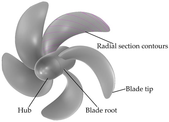
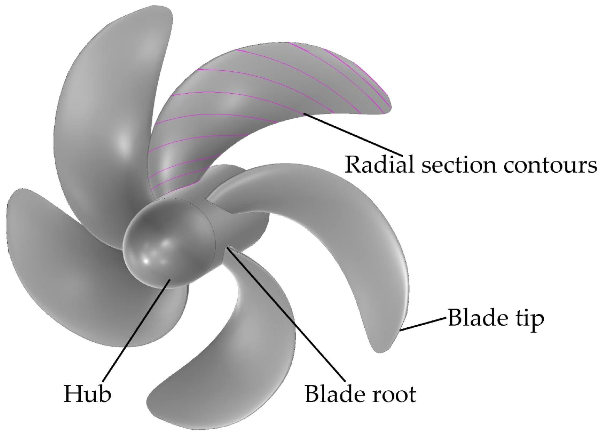
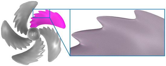
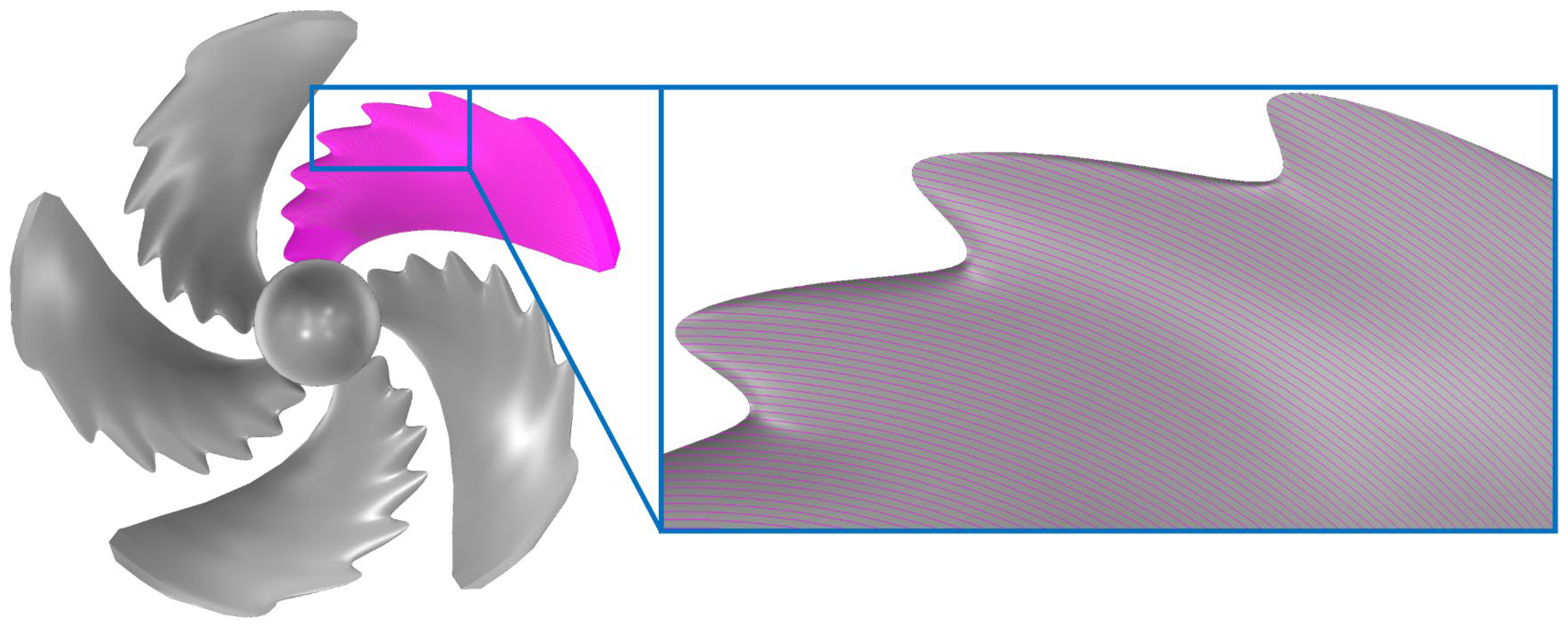
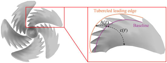
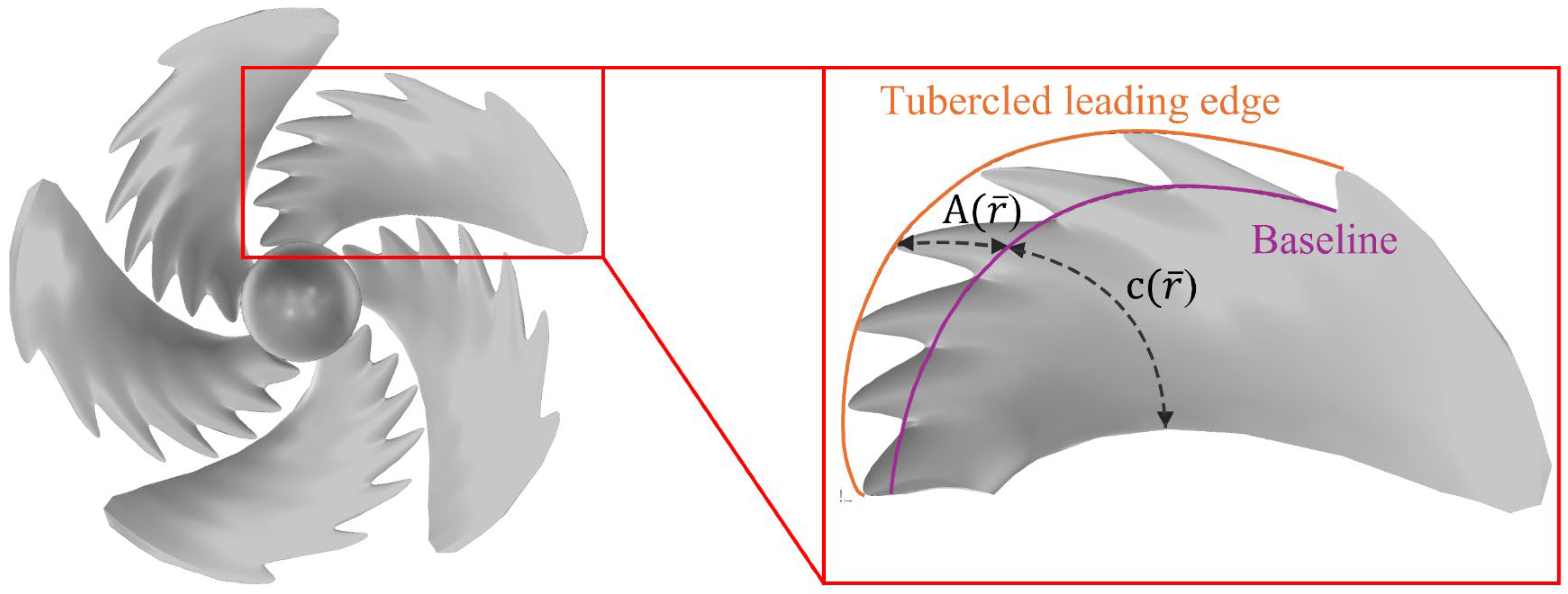
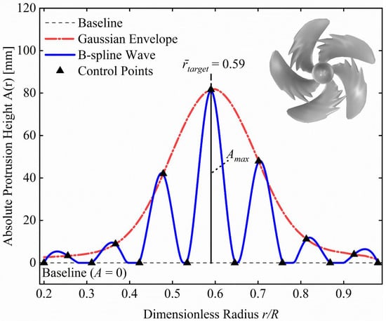
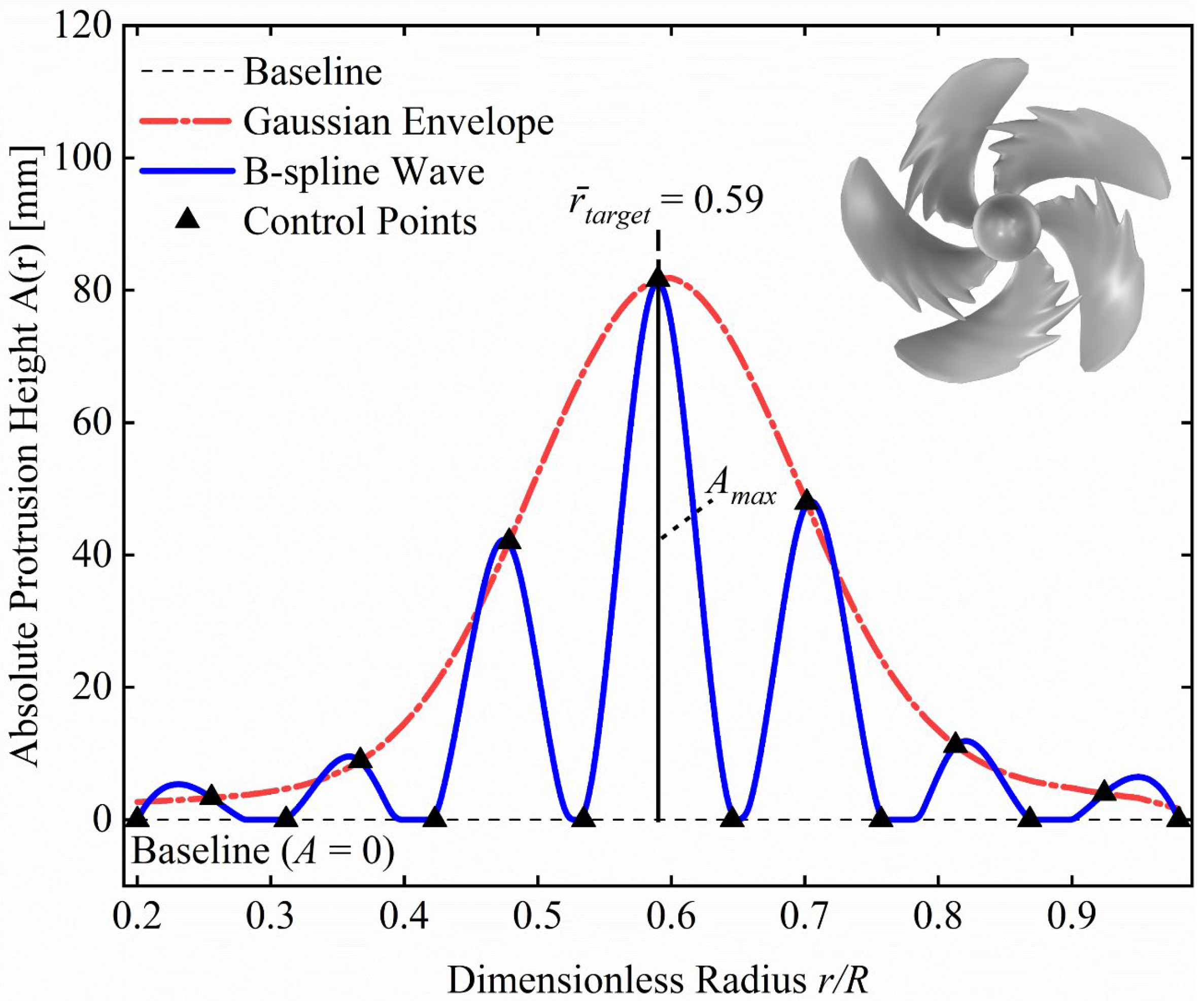
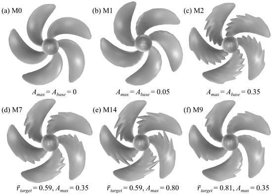
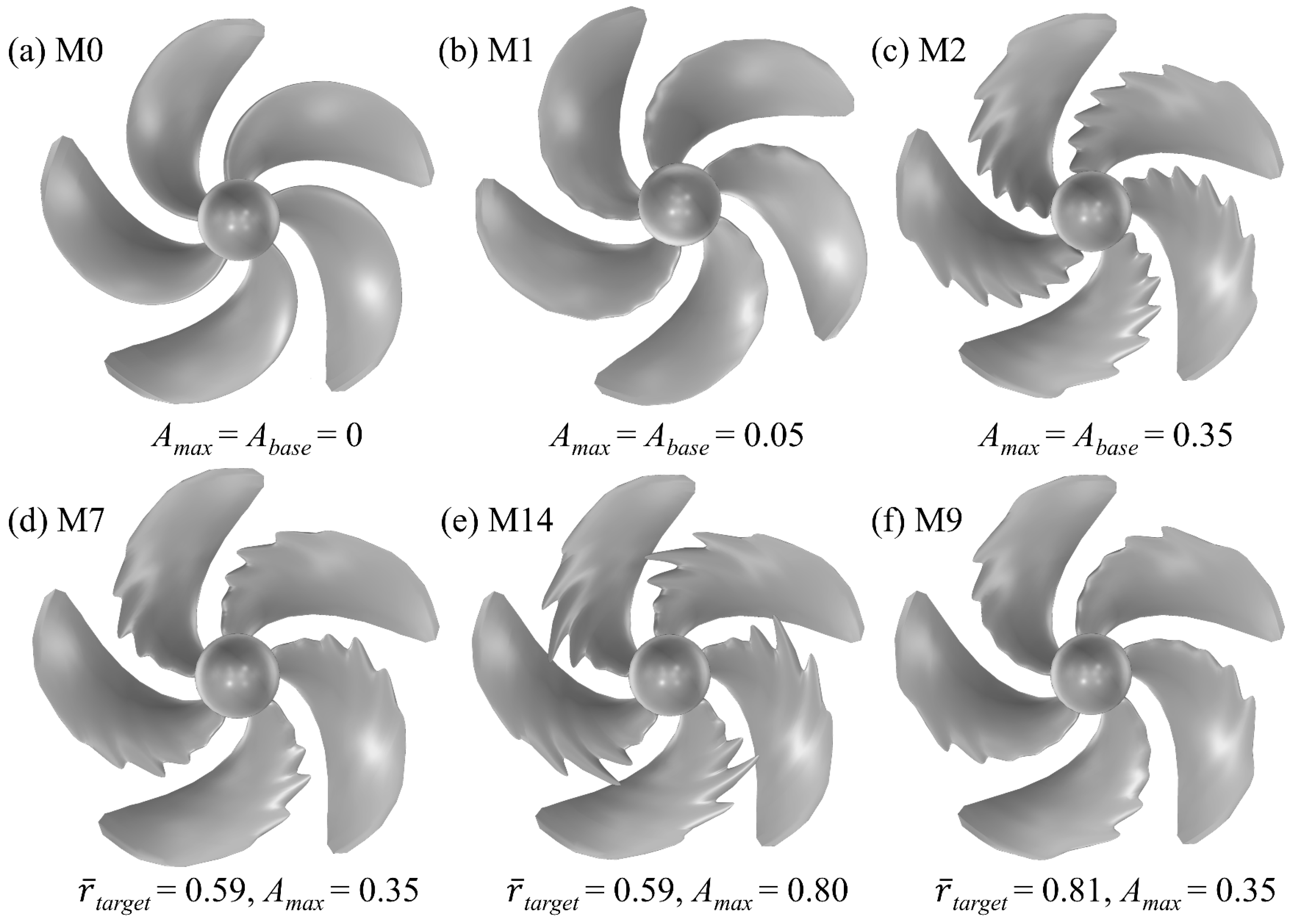
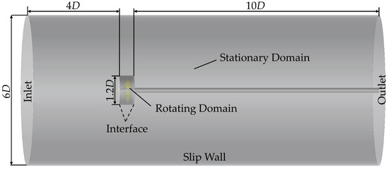
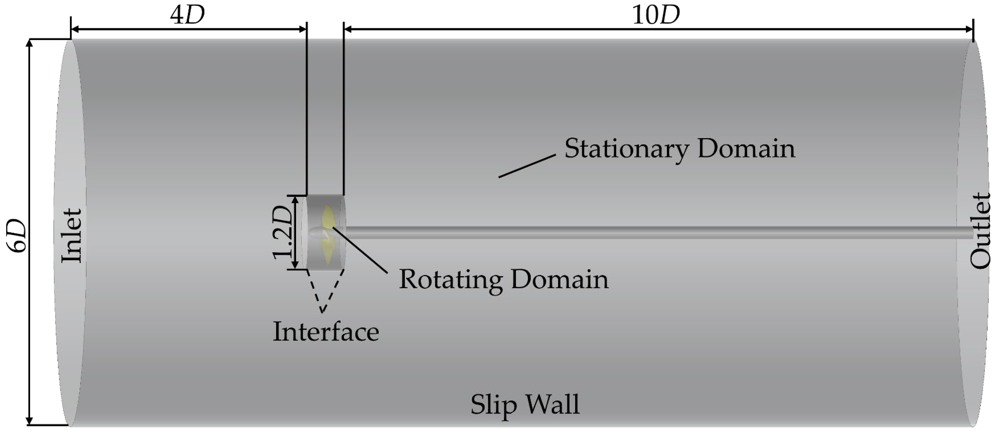
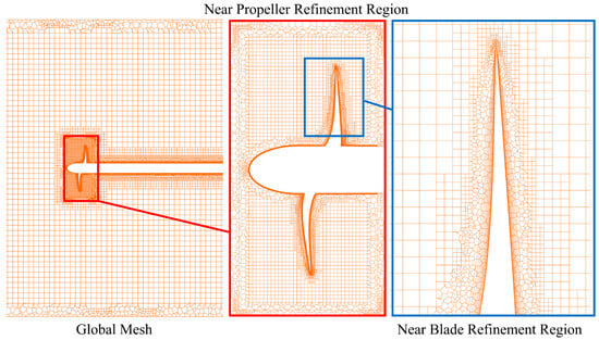
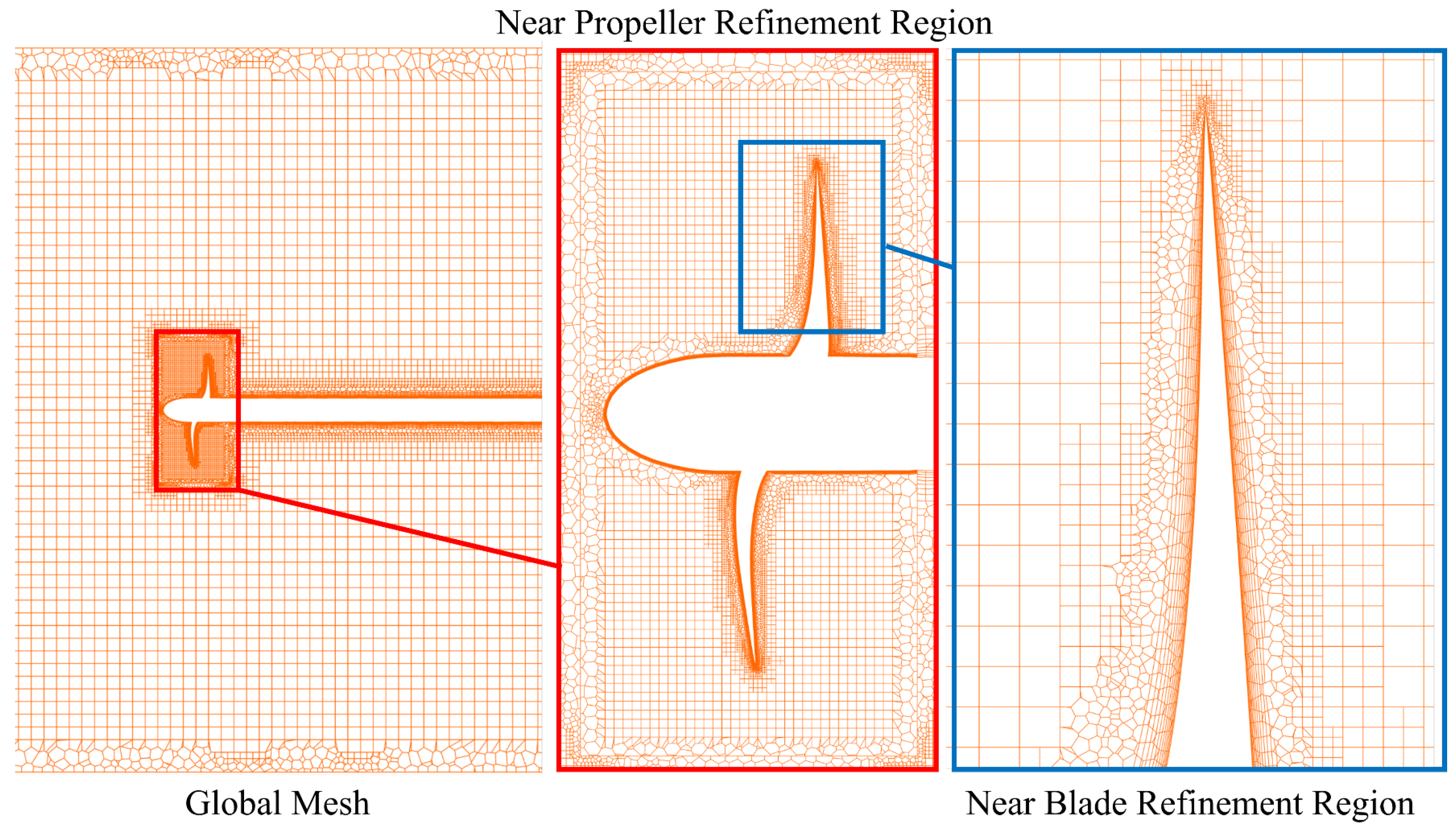
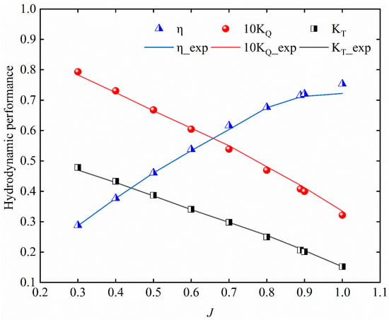
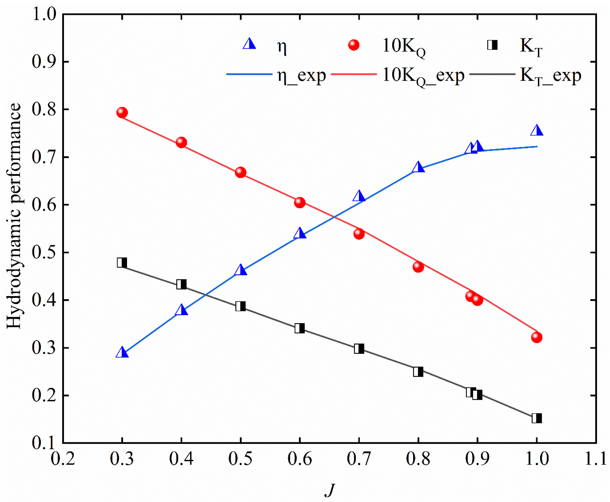
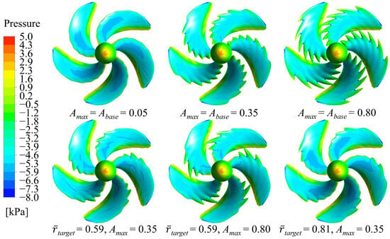
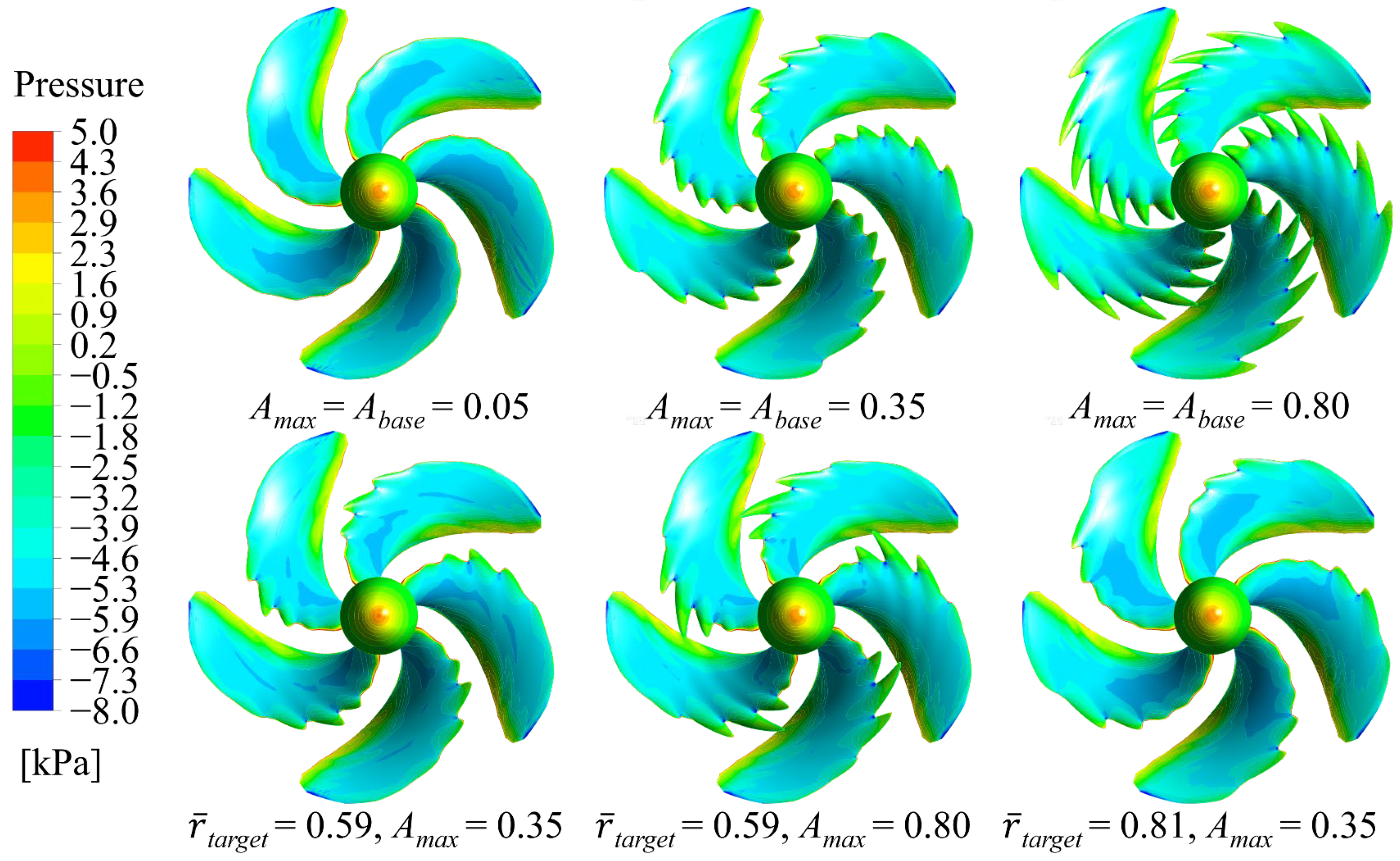
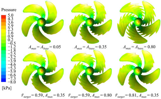
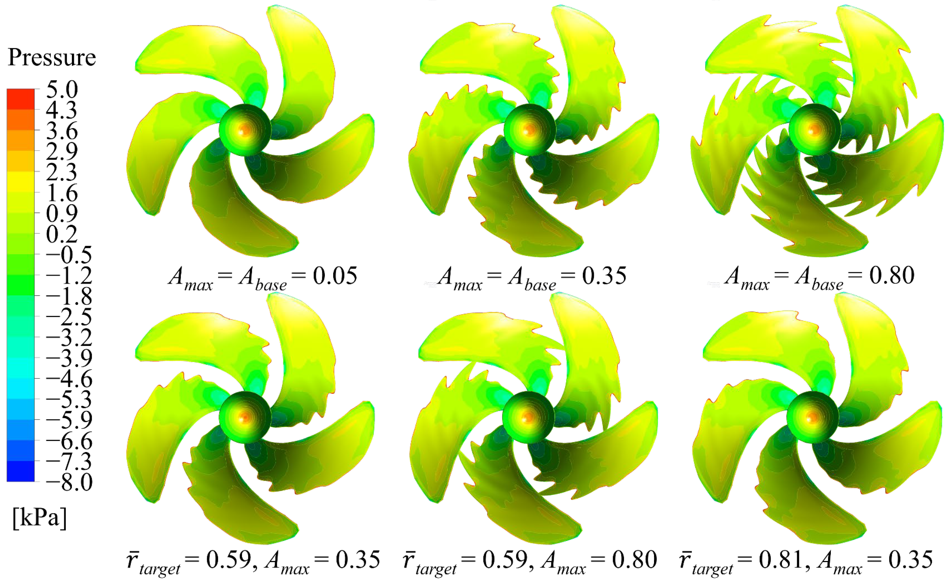
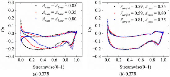
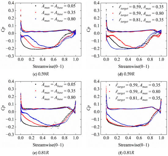
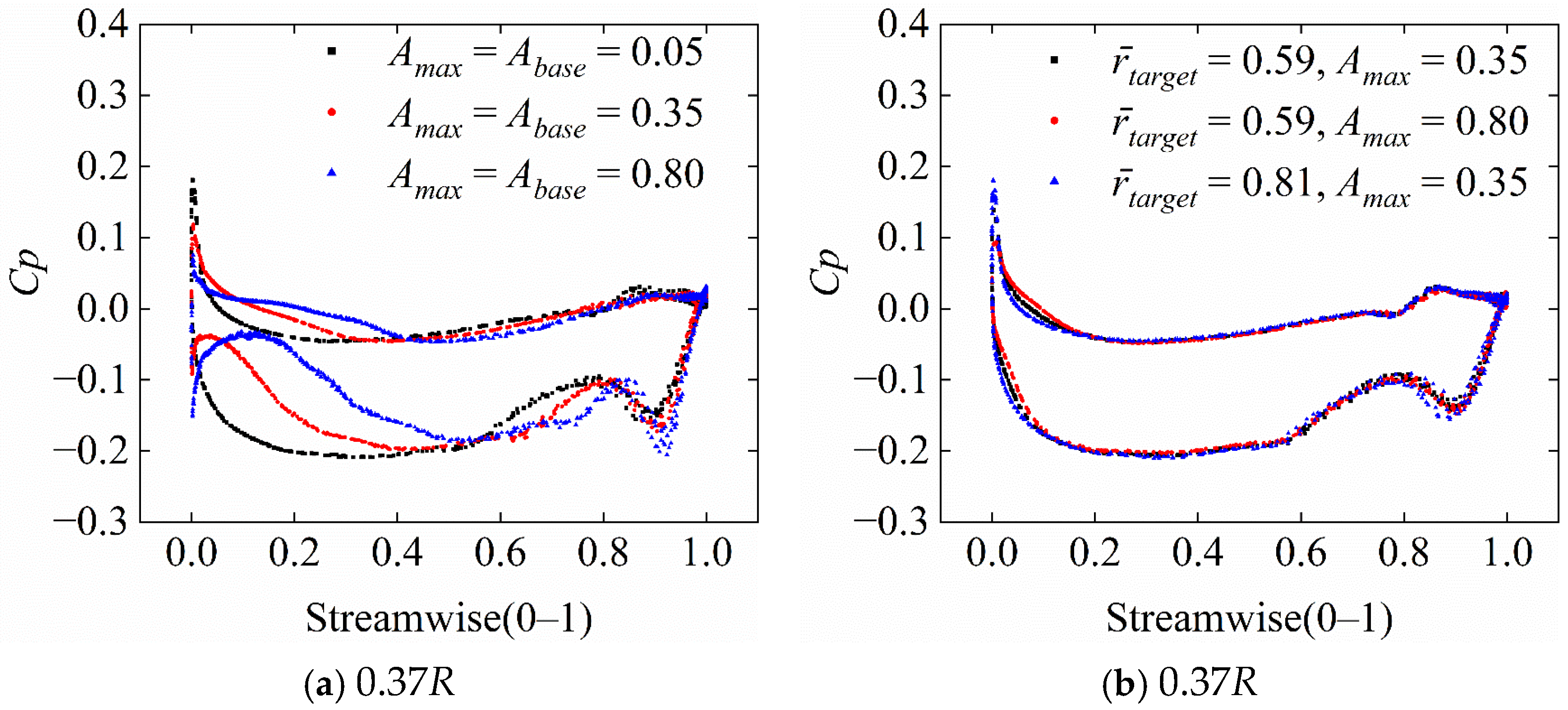
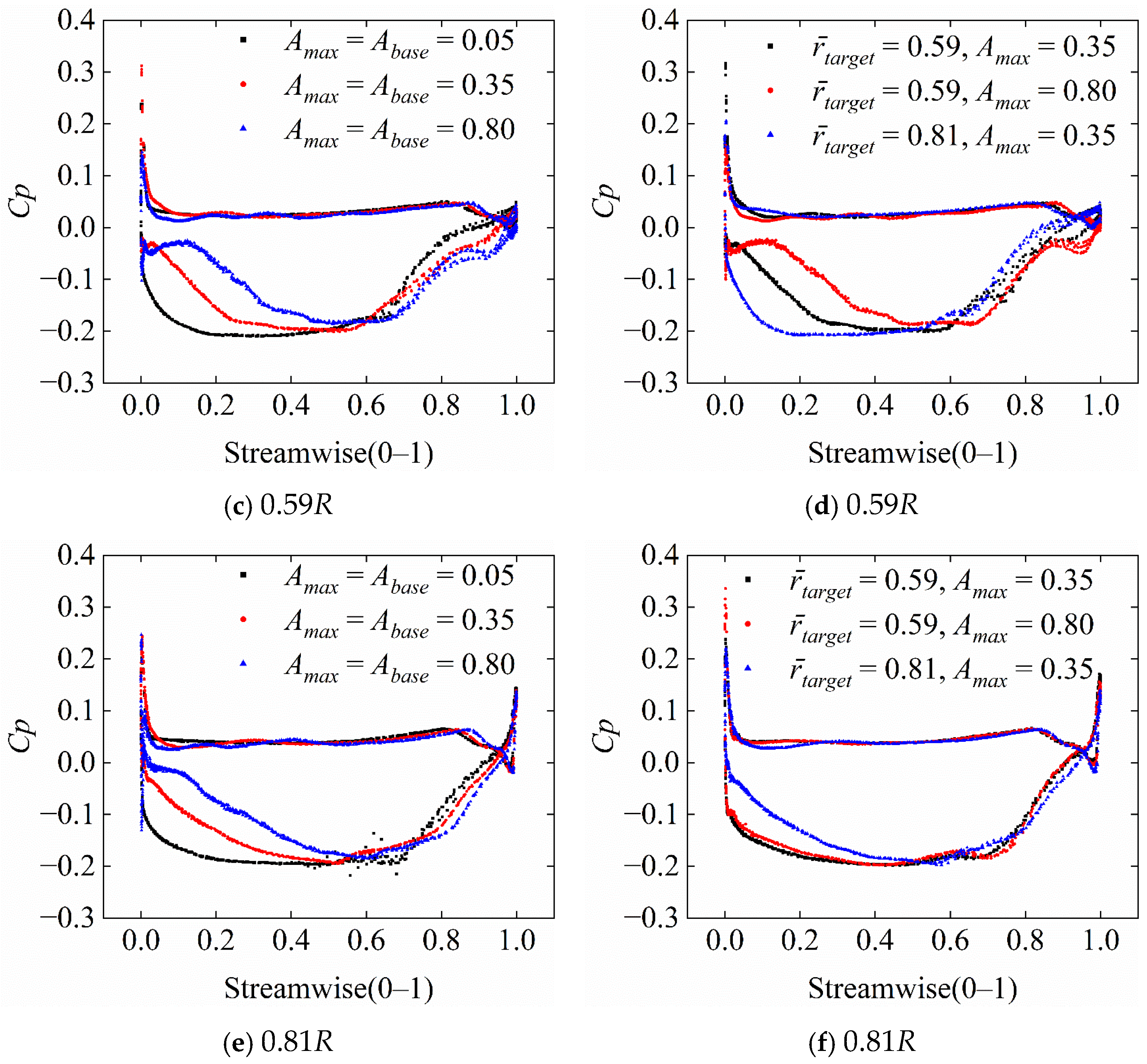
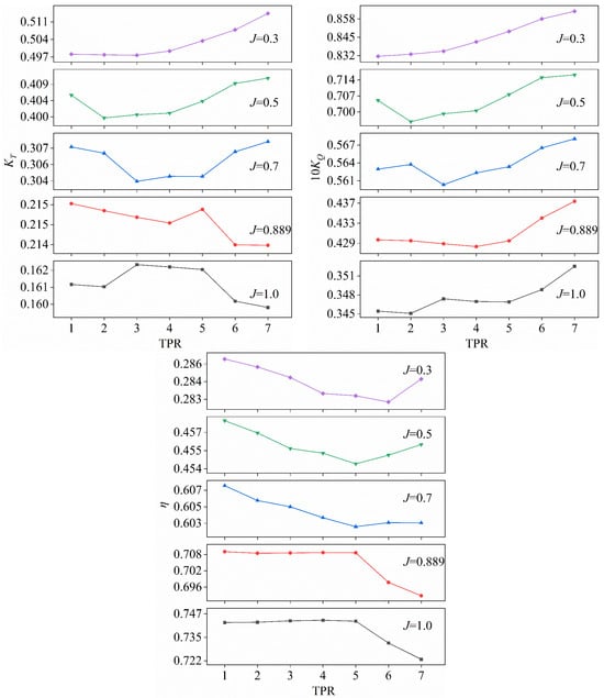
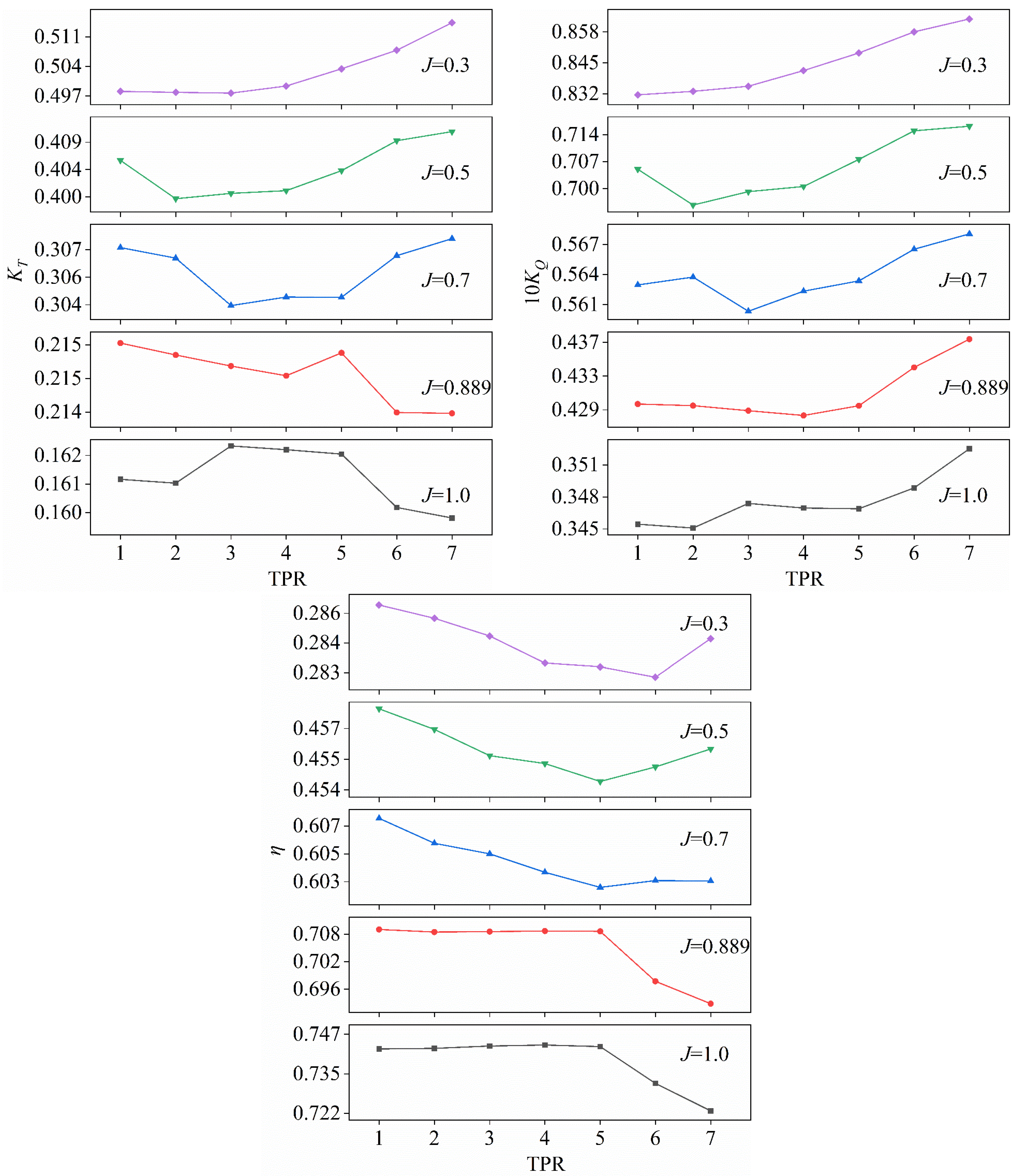
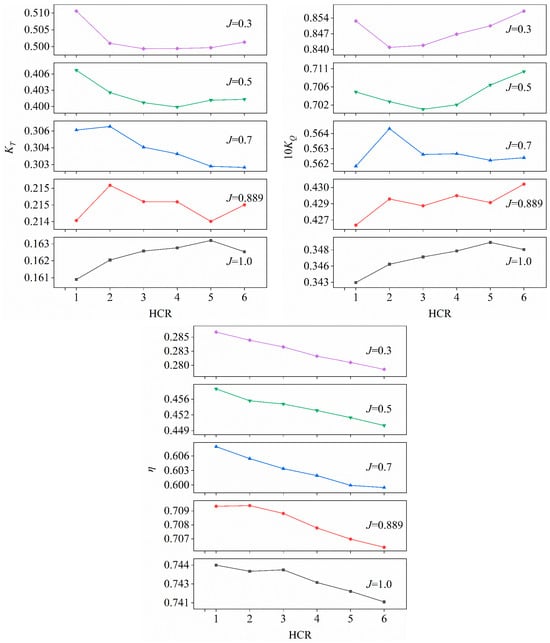
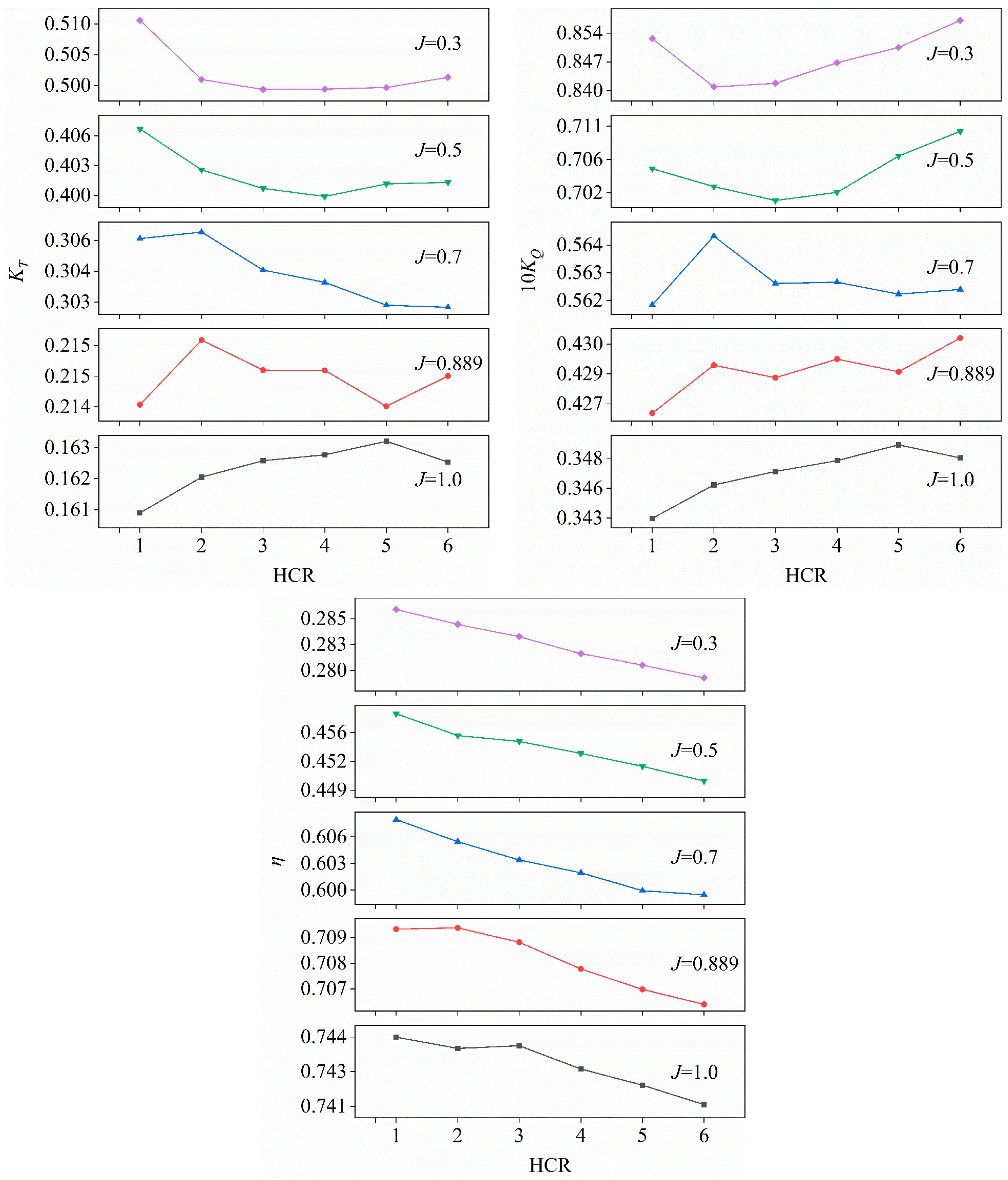

Disclaimer/Publisher’s Note: The statements, opinions and data contained in all publications are solely those of the individual author(s) and contributor(s) and not of MDPI and/or the editor(s). MDPI and/or the editor(s) disclaim responsibility for any injury to people or property resulting from any ideas, methods, instructions or products referred to in the content. |
© 2026 by the authors. Licensee MDPI, Basel, Switzerland. This article is an open access article distributed under the terms and conditions of the Creative Commons Attribution (CC BY) license.