Propagation-Time-Consistent Ray-Path Correction for Long-Baseline Underwater Acoustic Localization

Abstract

Non-uniform sound velocity profiles (SVPs) cause sound-ray refraction and propagation-path bending. The straight-line mapping among propagation time, propagation distance, and target position is, therefore, disrupted, leading to systematic errors in constant-sound-speed localization. To improve the consistency between propagation correction and geometric localization, an iterative ray-path correction method based on propagation-time consistency is proposed. The method contains three coupled steps. First, a path-dependent local layered SVP model is constructed for each target-to-base-station path, rather than using a global or fixed sound-speed model. Second, the ray parameter is inverted under the constraint of measured time-of-arrival (TOA), so that the corrected ray path remains consistent with the observed propagation time. Third, the corrected slant range obtained by layered ray tracing is fed back into a known-depth weighted least squares (WLS) localization model, forming a closed-loop position update. The method is evaluated through long-baseline (LBL) simulations with multiple SVPs and propagation geometries and is validated using measured TOA data and an observation-derived SVP. The simulation results show that sub-meter accuracy can be achieved under the tested TOA-noise conditions. In measured-data validation, the planar localization error is reduced from 4.6866 m to 0.1923 m. No divergence is observed in the tested small SVP-perturbation cases.

1. Introduction

With the development of deep-sea exploration, marine engineering surveying and mapping, seafloor observation networks, and underwater robotic technologies, high-precision underwater acoustic localization has become an important supporting technology for ocean observation and underwater operations [1]. In practical marine environments, underwater localization accuracy is affected not only by the geometry of base stations and the observation model. It is also strongly constrained by uncertainties in the acoustic propagation environment [2]. Moreover, the measurement and modeling accuracy of the sound velocity profile (SVP) directly affects the interpretation of propagation time, the construction of slant range, and the results of localization [3,4]. Therefore, improving the consistency between propagation modeling and geometric localization under non-uniform SVP conditions is one of the key issues in enhancing underwater acoustic localization accuracy [5,6].

In real marine environments, the SVP is jointly affected by temperature, salinity, and depth. It usually shows distinct vertical stratification characteristics [3]. The vertical variation of the SVP causes sound-ray refraction and propagation-path bending. As a result, the acoustic propagation time, geometric distance, and target spatial coordinates no longer satisfy the simple mapping relationship under ideal straight-line propagation conditions [7]. From the perspective of propagation modeling, ray acoustics models are based on geometrical acoustics and Snell’s law. They can describe the sound-ray propagation path, arrival time, and incident angle distribution. Therefore, they are suitable for propagation-path correction under non-uniform SVP conditions. Ray- and beam-based propagation models, such as BELLHOP, have been widely used for underwater acoustic propagation-path calculation and engineering simulation [7,8]. To address sound-ray path deviations caused by SVP non-uniformity, existing studies have used model-driven ray-tracing methods. These methods explicitly describe the influence of sound speed gradients on propagation paths. They can improve the modeling accuracy of propagation time and slant range [9]. In addition, adaptive layering methods can be used to adjust the layered structure according to variations in the sound speed gradient. This improves the environmental adaptability of ray tracing [10]. Moreover, under non-uniform SVP conditions, the time-of-arrival (TOA) observations and the geometric slant range no longer satisfy the simple linear mapping under the constant-sound-speed straight-line propagation assumption [11,12]. If the localization model still adopts a constant sound speed or straight-line propagation assumption, TOA observations are usually converted directly into geometric slant ranges. In this case, the propagation-path deviation caused by sound-ray bending appears as a ranging error. This error is further introduced into the geometric localization equations. It finally leads to bias in the estimated target position [13]. In addition to direct ray tracing, engineering approximation methods based on the effective sound velocity (ESV) or the average sound speed have also been widely used in underwater localization systems [14,15,16]. Existing studies have shown that methods based on in situ sound speed measurements, iterative ESV correction, and ESV table modeling can partly compensate for localization errors caused by sound speed variations. They can also improve computational efficiency in engineering applications [17,18,19]. However, ESV- or average-sound-speed-based methods still rely essentially on the equivalent-path assumption. Their correction performance is easily affected by SVP modeling accuracy, propagation-path variations, and the representation of sound speed gradients [20,21]. Ray-tracing methods can explicitly describe sound-ray bending [22]. However, if the ray parameters are mainly determined by the initial geometric relationship or empirical initial values, it is difficult to ensure consistency between the calculated sound-ray path and the actual TOA observations [23,24]. With the increasing requirement for system consistency in high-precision underwater localization, ray-path correction is gradually shifting from single propagation-path compensation to coupled modeling among sound speed parameters, propagation paths, and target positions [25,26]. Existing joint inversion studies have shown that simultaneous estimation of position parameters and sound speed perturbation information can reduce the systematic bias caused by stepwise processing. It can also improve the consistency of localization solutions [27]. Related studies further indicate that SVP uncertainty, propagation geometry, and target position estimation are strongly coupled [28,29]. However, joint optimization methods usually involve stronger nonlinearity and higher parameter dimensionality. In addition, practical underwater acoustic localization accuracy is jointly affected by the SVP structure, propagation path, and base-station geometry. Therefore, a trade-off is needed among SVP modeling, localization accuracy, and observation-geometry deployment [30,31]. From the perspective of error propagation, ray-path correction is not only a problem of improving the calculation accuracy of a single sound-ray path. It also concerns the consistency among SVP modeling, propagation-time interpretation, slant-range observation construction, and geometric localization. SVP errors affect ray parameters and propagation paths. Propagation-path deviations change the effective slant range corresponding to TOA observations [32,33]. The slant-range bias is then transformed into horizontal localization errors under the influence of the base-station geometry [34]. Without feedback to the localization model, one-time propagation compensation cannot fully suppress the transfer of SVP-induced slant-range errors to the position solution. In addition to propagation-layer errors, underwater acoustic localization is also affected by received-signal noise, multipath interference, array reception mismatch, and time synchronization errors [35].

Overall, existing methods still show a relative separation between propagation modeling and localization solution under non-uniform SVP conditions [36]. Conventional ray-tracing correction can describe propagation-path bending, but its ray parameters are usually determined by a given geometric relationship rather than directly constrained by measured TOA data. ESV- or local-average-sound-speed methods are efficient, but they still rely on equivalent sound-speed conversion and do not explicitly construct path-dependent corrected slant ranges. Full joint estimation methods provide stronger coupling between environmental and position parameters, but often require higher-dimensional nonlinear optimization. To address these limitations, this paper develops a lightweight closed-loop correction framework that combines path-dependent local SVP modeling, propagation-time-constrained ray inversion, and corrected-slant-range feedback within weighted least squares (WLS) localization. Its main algorithmic novelty is to feed TOA-consistent corrected slant ranges back into the localization model, thereby improving the coupling between ray-path modeling and position updating. The main contributions of this paper are as follows:

• A path-dependent local SVP layered modeling method is proposed. For different target-to-base-station propagation paths, the depth ranges crossed by sound rays are different. To address this issue, the local SVP between the target and each base station is extracted. A layered linear model is then used to describe the vertical variation of sound speed. This improves the path specificity and computability of propagation-path modeling.
• A ray-parameter solving method constrained by propagation-time consistency is proposed. A propagation-time consistency equation is constructed. The one-way propagation time corresponding to the TOA observation is introduced into the ray-parameter inversion process. In this way, ray-parameter solving is constrained by both the local SVP and the observed propagation time. This enhances the consistency between the ray-path correction result and the actual propagation time.
• A weighted least squares (WLS) localization framework with corrected-slant-range feedback is constructed. The corrected slant ranges obtained by layered ray tracing are continuously fed back into the known-depth WLS localization model. During the iterative process, the propagation geometry, ray parameters, slant-range observations, and target position are jointly updated. This improves the consistency among the propagation model, slant-range construction, and geometric localization updating.

2. Materials and Methods

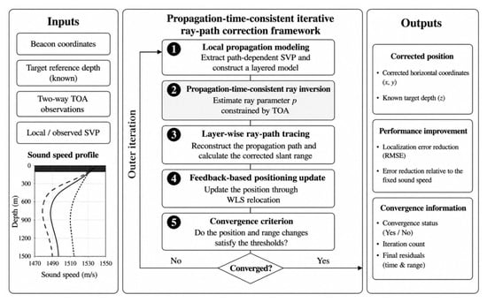
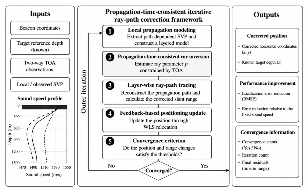
This paper proposes a propagation-time-consistent iterative ray-path correction method for known-depth two-dimensional long-baseline (LBL) localization, as shown in Figure 1. For each target-to-base-station path, a local layered SVP model is constructed, and the measured TOA is introduced into ray-parameter inversion through the propagation-time consistency equation. The corrected slant ranges obtained by layered ray tracing are then fed back into the WLS localization model, forming a closed-loop update among ray-parameter solving, slant-range correction, and geometric localization. Here, the efficiency of the propagation-time-consistent ray inversion is evaluated by the convergence of the propagation-time residual, the Newton iteration count, the feasibility of the solved ray parameter, and the stability of the corrected slant-range feedback.

Figure 1. Overall framework of the proposed iterative ray-path correction localization method.

2.1. Path-Dependent Local SVP Modeling

A two-dimensional LBL localization problem with known target depth is considered. The localization system is assumed to consist of $N$ fixed receiving base stations. The three-dimensional coordinates of base station $i$ are given by

$$a_i={[x_i,y_i,z_i]}^T,\hspace{1em}i=1,2,\dots ,N$$

(1)

where $x_i$ and $y_i$ denote the horizontal coordinates of base station $i$ and $z_i$ denotes its depth coordinate. The position of the sound source to be localized is expressed as

$$s={[x,y,z_0]}^T$$

(2)

where $z_0$ is the target depth. In this paper, the target depth is assumed to be obtained from a pressure sensor or prior information. Therefore, the unknown localization variable is the horizontal target position,

$$\xi ={[x,y]}^T$$

(3)

For the $i\text{-}th$ target-to-base-station propagation path, the measured two-way propagation time is denoted as ${\tau }_i$. The corresponding one-way propagation time is ${\tau }_i/2$. Traditional constant-sound-speed or global-SVP modeling usually applies the same sound speed model to all propagation paths. However, the depth span and propagation geometry between different base stations and the target are not the same. To highlight the local sound speed characteristics of each propagation path, this paper extracts the path-related local SVP according to the target depth and the base-station depth. Its depth range is defined as

$$[z_{\min ,i},z_{\max ,i}]=[\min (z_0,z_i),\max (z_0,z_i)]$$

(4)

If an endpoint depth is not located on the original SVP sampling grid, linear interpolation is used only to obtain the sound speed at that endpoint, while all original SVP samples within the local depth interval are retained. After endpoint interpolation and local extraction, the local SVP corresponding to the $i\text{-}th$ path can be expressed as

$$C_i={\{(z_{i,l},c_{i,l})\}}_{l=0}^{L_i}$$

(5)

where $z_{i,l}$ and $c_{i,l}$ denote the $l\text{-}th$ depth node and its sound speed in the local SVP of the $i\text{-}th$ path, respectively. $L_i$ is the number of layers in the local profile and is determined by the SVP samples retained between $z_0$ and $z_i$. Thus, the local profile contains $L_i+1$ depth nodes and $L_i$ layers. $N$ denotes the number of receiving base stations, equivalently the number of TOA observations used for localization; in this study, $N=4$ for both the simulation and measured-data cases. The endpoint interpolation is used only to obtain the sound speed at the boundary depths and does not replace the layer-wise SVP model. For coarsely sampled or strongly varying SVPs, denser SVP measurements or higher-order local interpolation can be adopted to improve the endpoint sound-speed estimation without changing the subsequent layer-wise ray-tracing framework.

$$c_{i,l}(z)=c_{i,l}+g_{i,l}(z-z_{i,l}),\hspace{1em}z\in [z_{i,l},z_{i,l+1}]$$

(6)

where $g_{i,l}$ is the sound speed gradient in layer $l$. The layered linear sound speed model is a common propagation modeling approach in ray acoustics. This paper does not further expand the complete analytical integration of the in-layer propagation time and horizontal distance. Instead, it uses this model as the basis for subsequent ray-parameter inversion and layered ray tracing. Unlike global-profile modeling, the proposed approach adaptively extracts a path-dependent local SVP for each target-to-base-station path. Thus, each path is associated with its own layered sound-speed environment, which improves the path specificity of subsequent ray-parameter inversion and ray tracing.

2.2. Propagation-Time-Consistent Ray-Parameter Inversion

Given the local SVP and ray parameters, conventional ray-tracing methods can calculate the one-way propagation time from the target depth to the base-station depth. Unlike methods that determine ray parameters directly from the initial geometric relationship, the measured TOA is introduced into the ray-parameter solving process. This ensures consistency between the calculated propagation time and the observed propagation time.

Let the ray parameter of the $i\text{-}th$ path be $p_i$. The one-way propagation time calculated from the local SVP is denoted as $T_i(p_i)$. This paper constructs the propagation-time consistency equation as

$$F_i(p_i)=T_i(p_i)-{\displaystyle \frac{{\tau }_i}{2}}=0$$

(7)

where $F_i(p_i)$ is the propagation-time residual. When $F_i(p_i)=0$, the one-way propagation time calculated under the current ray parameter is consistent with the one-way propagation time corresponding to the TOA observation. This equation is the key constraint that distinguishes the proposed ray-path correction method from conventional geometric ray correction.

Because the analytical derivative of $T_i(p_i)$ with respect to $p_i$ is complicated under a layered linear SVP, this paper uses a finite-difference Newton method to solve Equation (7):

$$p_i^{(n+1)}=p_i^{(n)}-{\displaystyle \frac{F_i(p_i^{(n)})}{F_{i^{\prime }}(p_i^{(n)})}}$$

(8)

where $n$ is the Newton iteration index, and $F_i^{\prime }(p_i^{(n)})$ is approximated by numerical finite differences. In the implementation, the Newton iteration is terminated when the absolute propagation-time residual satisfies $|F_i(P_i)|<{\epsilon }_T$, where ${\epsilon }_T=1\times {10}^{-5}$ s is used as the ray-parameter inversion tolerance. To ensure that the ray parameter has physical meaning, a feasible-domain constraint is imposed on $p_i$ during the solving process. Numerical protection is also applied when the difference point crosses the boundary, the propagation time is invalid, or the derivative is too small. The Newton iteration described above is a conventional tool for solving nonlinear equations. The core of this paper is not to modify the Newton method. Instead, the measured TOA is used as a constraint for ray-parameter inversion. In this way, the ray parameter is constrained by both the local SVP and the measured propagation time.

After obtaining the ray parameter that satisfies propagation-time consistency, layered ray tracing [37] is used to calculate the accumulated horizontal displacement and vertical displacement of the corresponding path. In the $k\text{-}th$ outer iteration, let the horizontal displacement obtained by ray tracing for the $i\text{-}th$ path be $x_i^{(k)}$, and let the vertical displacement be $z_i^{(k)}$. The corrected slant range is then defined as

$$R_{i,\mathrm{ray}}^{(k)}=\sqrt{{(x_i^{(k)})}^2+{(z_i^{(k)})}^2}$$

(9)

Relation (9) is introduced because the WLS localization module requires a slant-range observation between the target and each base station. After the ray parameter is constrained by Equation (7), layer-wise ray tracing provides the accumulated horizontal and vertical endpoint displacements of the corresponding path. Therefore, is computed from these two displacements and used as a WLS-compatible corrected slant range, rather than as a constant-sound-speed TOA-derived range. The accuracy of this constraint is evaluated by the corrected-range closure error and the propagation-time residual. In the numerical closure test, the endpoint residuals, corrected-range error, and Newton time-integration residual remain at very low levels, confirming the consistency of Equation (9) with the TOA-constrained ray-tracing result.

2.3. Weighted Least Squares (WLS) Localization Update with Corrected-Slant-Range Feedback

The weighted least squares (WLS) method is a commonly used position-solving method in underwater geometric localization. This paper does not rederive the complete Gauss–Newton solution process of WLS. Instead, WLS is used as a geometric localization module. The focus is on constructing the feedback mechanism from the corrected slant range to the WLS localization model.

In the initial stage, the sound speed near the target depth, $c(z_0)$, is used to convert the two-way propagation time into the initial slant range:

$$R_i^{(0)}={\displaystyle \frac{c(z_0){\tau }_i}{2}}$$

(10)

This initial slant range corresponds to the constant-sound-speed straight-line propagation assumption. It is only used to obtain the initial localization result and is not used as the final ranging result. For the current estimate of the horizontal target position, $\xi ={[x,y]}^T$, the predicted three-dimensional geometric range between the target and base station $i$ is given by

$${\widehat{R}}_i(x,y)=\sqrt{{(x-x_i)}^2+{(y-y_i)}^2+{(z_0-z_i)}^2}$$

(11)

Here, ${\widehat{R}}_i(x,y)$ is referred to as the geometric slant range because it includes both the horizontal separation and the depth difference between the target and the base station. It is therefore different from the horizontal range, but it is not the curved acoustic ray-path length. Given the slant-range observation $R_i$ used for the current localization solution, the WLS localization objective function is written as

$$J(x,y)={\displaystyle \sum _{i=1}^N{w}_i}{\left[R_i-{\widehat{R}}_i(x,y)\right]}^2$$

(12)

where $w_i$ is the weight of the $i\text{-}th$ slant-range observation. In the present simulations and measured-data validation, equal weights are used because reliable link-specific TOA variances or signal-to-noise ratio (SNR)-based confidence indicators are not available for all observations. This setting also avoids introducing an additional weighting assumption and allows the comparison to focus on the effect of slant-range correction. When reliable TOA uncertainty estimates are available, the weight matrix can be defined according to the inverse variance of each TOA or range observation.

To reduce the influence of abrupt slant-range variations in the outer iteration on the WLS solution, a smoothed feedback strategy is adopted for the corrected slant range:

$$R_i^{(k+1)}=\alpha R_i^{(k)}+(1-\alpha )R_{i,\mathrm{ray}}^{(k)}$$

(13)

where $\alpha$ is the slant-range smoothing factor, $R_i^{(k)}$ is the slant range used for WLS localization in the $k\text{-}th$ outer iteration, and $R_{i,\mathrm{ray}}^{(k)}$ is the corrected slant range obtained by ray tracing. Through Equation (13), the initial slant range under the constant-sound-speed assumption is gradually corrected into a slant-range observation that is more consistent with the local SVP and the TOA constraint.

After the slant ranges of all base stations are updated, a new slant-range observation vector is formed as

$$R^{(k+1)}={[R_1^{(k+1)},R_2^{(k+1)},\dots ,R_N^{(k+1)}]}^T$$

(14)

By inputting $R^{(k+1)}$ into the WLS localization model, a new estimate of the target horizontal position, ${\xi }^{(k+1)}$, can be obtained. Therefore, the outer closed loop of the proposed method can be summarized as

$${\xi }^{(k)}\to {\left\{p_i^{(k)}\right\}}_{i=1}^N\to {\left\{R_{i,\mathrm{ray}}^{(k)}\right\}}_{i=1}^N\to R^{(k+1)}\to {\xi }^{(k+1)}$$

(15)

Equation (15) reflects the main innovation of the proposed method. The ray parameters, corrected slant ranges, and target position are not calculated separately in a stepwise manner. Instead, they are coupled in a closed loop during the outer iteration. The convergence criteria for the outer iteration are defined as

$$\Delta R_{\max }^{(k)}<{\epsilon }_R\hspace{1em}\mathrm{or}\hspace{1em}\Delta {\xi }^{(k)}<{\epsilon }_{\xi }$$

(16)

In this study, the maximum number of outer iterations is set to $K_{\max }=30$. If neither convergence criterion in Equation (16) is satisfied before reaching $K_{\max }$, the iteration is stopped and the latest valid estimate is retained. The slant-range variation $\Delta R_{\max }^{(k)}$ evaluates the convergence of the propagation-correction layer, whereas the position variation $\Delta {\xi }^{(k)}$ evaluates the stability of the WLS localization update. Therefore, the iteration is regarded as converged when either the corrected slant ranges or the position estimate becomes sufficiently stable. Numerical protection is applied if ray-parameter solving fails, ray tracing becomes invalid, or the WLS normal matrix is close to singular. A rank-deficient design matrix or an ill-conditioned normal matrix indicates weak geometric observability, which may amplify small slant-range residuals and cause unstable position updates. In such cases, a Moore–Penrose pseudo-inverse is used, and if the update remains unstable, the latest valid position and slant ranges are retained to avoid divergence. Overall, the proposed method transforms one-time propagation compensation into a feedback-based localization observation update.

2.4. Iterative Ray-Path Correction Localization Procedure

Table 1 summarizes the complete iterative procedure of the proposed method, from initial slant-range construction to TOA-constrained ray tracing, corrected-slant-range feedback, and WLS localization updating.

Table 1. Flowchart of the iterative ray-path correction localization algorithm based on propagation-time consistency.

Step	Operation
Input	Base-station coordinates ${\left\{a_i\right\}}_{i=1}^N,$ target depth $z_0,$ two-way propagation times ${\left\{{\tau }_i\right\}}_{i=1}^N,$ SVP $C$ initial position ${\xi }^{(0)},$ maximum number of iterations $K_{\max },$ convergence thresholds ${\epsilon }_R$ and ${\epsilon }_{\xi },$ and smoothing factor $\alpha$
1	Construct the initial slant ranges $R_i^{(0)}$ using the sound speed at the target depth, $c_{z(0)},$ and the two-way propagation times ${\left\{{\tau }_i\right\}}_{i=1}^N.$
2	Solve the initial WLS position using the initial slant ranges ${\left\{R_i^{(0)}\right\}}_{i=1}^N$ and the known target depth $z_0.$
3	In the $k\text{-}th$ outer iteration, calculate the propagation geometry for each target-to-base-station path according to the current target position ${\xi }^{(k)}.$
4	Extract the local SVP between the target depth $z_0$ and the base-station depth $z_i$ for each path. Construct a layered linear propagation model.
5	Solve the propagation-time consistency equation $T_i(p_i)-{\displaystyle \frac{{\tau }_i}{2}}=0,$ and obtain the ray parameter $p_i^{(k)}.$
6	Perform layered ray tracing based on $p_i^{(k)},$ and calculate the corrected slant range.
7	Update the slant range using the smoothed feedback strategy, $R_i^{(k+1)}=\alpha R_i^{(k)}+(1-\alpha )R_{i,\mathrm{ray}}^{(k)}.$
8	Input the updated slant-range vector $R^{(k+1)}$ into the WLS localization model and solve the new target position ${\xi }^{(k+1)}.$
9	Calculate the maximum slant-range variation $\Delta R_{\max }^{(k)}$ and the position variation $\Delta {\xi }^{(k)}.$
10	If $\Delta R_{\max }^{(k)}<{\epsilon }_R$ or $\Delta {\xi }^{(k)}<{\epsilon }_{\xi },$ stop the iteration. Otherwise, return to Step 3.
Output	Estimated horizontal target position $\widehat{\xi },$ corrected slant-range sequence, number of iterations, and convergence status.

3. Simulation Validation and Performance Analysis

3.1. Simulation Scenarios and TOA Forward Modeling

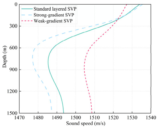
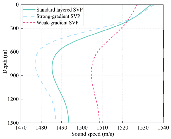
To validate the influence of ray-path correction on LBL localization accuracy under non-uniform SVP conditions, this paper constructs multiple types of SVPs and multi-base-station localization geometries. The simulated SVPs are shown in Figure 2. They include a standard layered SVP, a strong-gradient SVP, and a weak-gradient SVP. These profiles are used to represent a typical layered ocean environment, an environment with significant sound-ray bending, and an approximately uniform propagation environment, respectively. By changing the strength of the sound speed gradient, the effects of vertical SVP variation on the propagation path, effective sound speed, and localization error are analyzed. Existing studies have shown that SVP measurement, layered modeling, and sound speed gradient representation all affect the interpretation of underwater acoustic propagation time and localization results [3,10,21]. Therefore, comparative validation under different SVP structures is necessary. It should be noted that all simulation scenarios and field experiments in this study were conducted with the target located inside the sensor network.

Figure 2. Smoothed theoretical SVPs.

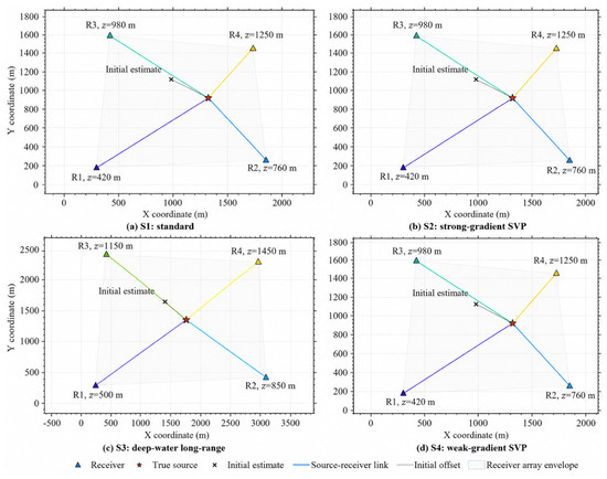
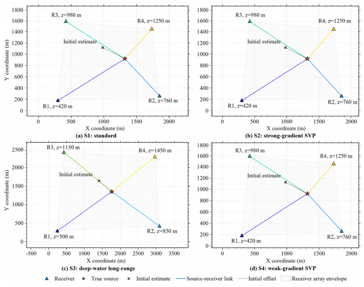
On this basis, four LBL simulation scenarios are designed, as shown in Figure 3. The source–receiver geometry affects signal propagation through the horizontal propagation distance, the depth difference between the source and each receiver, and the corresponding local SVP interval. S1 is used as the standard baseline scenario, while S2 and S4 use similar geometries to examine the influence of strong- and weak-gradient SVPs, respectively. S3 represents a deep-water long-range geometry with larger propagation distances and deeper receivers. These scenarios provide unified simulation inputs for evaluating the proposed method under different SVP structures, propagation scales, base-station depth distributions, and initial localization biases.

Figure 3. Multi-scenario source–receiver geometries used in the simulation validation.

S1, S2, and S4 use similar geometries to compare the effects of different SVP gradients, whereas S3 represents a deep-water long-range geometry. Receiver depths, source–receiver links, and initial-position offsets are shown to illustrate the horizontal propagation distances and vertical depth spans used for local SVP extraction and ray-path correction.

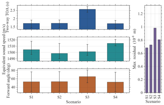
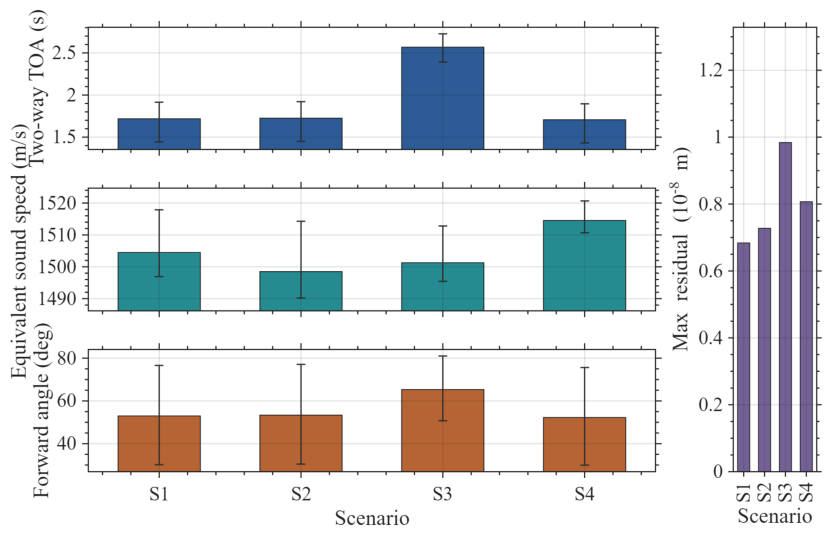
To ensure that the observations are consistent with the propagation mechanism under non-uniform SVP conditions, this paper uses a ray-based forward modeling method to generate two-way TOA observations. This treatment is consistent with existing ray-tracing localization studies, where localization observations are corrected through layered propagation models, incident-angle calculation, and path tracing [23,32]. For each source-to-base-station path, the ray parameter satisfying the propagation-time consistency constraint is inverted based on the true geometry and the layered SVP. The two-way propagation time, forward incident angle, and path effective sound speed are then calculated. Figure 4 shows clear path-dependent differences in two-way propagation time and effective sound speed, which cannot be accurately represented by a single constant sound speed.

Figure 4. TOA forward-modeling diagnostic results under multi-scenario non-uniform SVPs.

The corresponding simulation scenario settings and validation purposes are summarized in Table 2.

Table 2. Simulation scenario settings and validation purposes.

Scenario	SVP Type	Scenario Characteristics	Validation Purpose
S1 standard	Standard layered SVP	Typical layered propagation	Baseline performance validation
S2 strong	Strong-gradient SVP	Strong refractive environment	Gradient sensitivity analysis
S3 deep	Deep-water SVP	Long-range deep-water geometry	Robustness under deep-water propagation
S4 weak	Weak-gradient SVP	Near-uniform propagation	Applicability under weak refraction

Meanwhile, the horizontal-distance matching residuals of the forward rays remain at the order of 10⁻⁹–10⁻⁸, confirming the numerical consistency of the constructed observations. Thus, subsequent localization errors mainly originate from SVP modeling, ray-path correction, and geometric inversion rather than TOA forward-modeling errors.

3.2. Performance Analysis of Complete Ray-Path Correction Localization

To quantitatively evaluate the localization performance, this paper mainly uses planar localization error, error reduction rate, root mean square error (RMSE), standard deviation, posterior unit weight standard deviation, dilution of precision (DOP), and iterative convergence quantities as evaluation metrics. Let the true horizontal position of the target be

$$P_{true}={\left[x_{true},y_{true}\right]}^T$$

(17)

The planar position estimate output by the localization algorithm is

$$\widehat{P}={\left[\widehat{x},\widehat{y}\right]}^T$$

(18)

The errors in the $X$ and $Y$ directions and the planar Euclidean error are defined as

$$e_x=\widehat{x}-x_{true},e_y=\widehat{y}-y_{true},e=\sqrt{e_x^2+e_y^2}$$

(19)

The error reduction rate is defined as

$$\eta ={\displaystyle \frac{e_{before}-e_{after}}{e_{before}}}\times 100\%$$

(20)

For multiple groups of experiments, let the planar Euclidean error of the $q\text{-}th$ group be $e_q$, and let the number of experimental groups be $Q$. Then, the mean error, RMSE, and standard deviation are defined as

$$\begin{array}{l}\overline{e}={\displaystyle \frac{1}{Q}}{\displaystyle \sum _{q=1}^Q{e}_q}\\ RMSE=\sqrt{{\displaystyle \frac{1}{Q}}{\displaystyle \sum _{q=1}^Q{e}_q^2}}\\ s_e=\sqrt{{\displaystyle \frac{1}{Q-1}}{\displaystyle \sum _{q=1}^Q{\left(e_q-\overline{e}\right)}^2}}\end{array}$$

(21)

In addition, the posterior unit weight standard deviation σ is used to characterize the residual consistency between the slant-range observations and the WLS geometric localization model:

$$\sigma =\sqrt{{\displaystyle \frac{v^{T}Wv}{N-2}}}$$

(22)

where $v$ is the residual vector after WLS localization, $W$ is the weight matrix, and $N$ is the number of base stations. To assist in judging whether the localization accuracy difference is caused by changes in base-station geometry, this paper uses a two-dimensional DOP metric:

$$DOP=trace\left[{\left(B^{T}WB\right)}^{-1}\right]$$

(23)

where $B$ is the WLS linearized design matrix. If $B$ is rank-deficient or the corresponding normal matrix is severely ill-conditioned, the DOP value becomes very large or unreliable, indicating poor geometric observability. In such cases, the localization result may be dominated by geometric amplification rather than by propagation-correction accuracy alone. If the DOP values of different methods are basically the same under the same base-station configuration and similar localization regions, the difference in localization error mainly comes from slant-range observation correction rather than geometric configuration changes.

To analyze the convergence behavior of the outer iteration, the maximum slant-range variation and position variation after each iteration are recorded as

$$\begin{array}{l}\Delta R_{\max }^{(k)}=\underset{i}{\max }\left|R_i^{(k+1)}-R_i^{(k)}\right|\\ \Delta {\xi }^{(k)}=‖{\widehat{p}}^{(k+1)}-{\widehat{p}}^{(k)}‖\end{array}$$

(24)

where $\Delta R_{\max }^{(k)}$ is used to characterize the convergence degree of the corrected slant ranges, and $\Delta {\xi }^{(k)}$ is used to characterize the stability of the localization result. For each iterative run, the maximum and minimum values of $\Delta R_{\max }^{(k)}$ and $\Delta {\xi }^{(k)}$ are recorded over the whole outer-iteration sequence. The maximum values reflect the initial correction magnitude, whereas the minimum values indicate the final convergence level.

These metrics are used to characterize all inversion results in a uniform manner. Specifically, localization accuracy is described by planar error or RMSE, correction performance by error-reduction rate, residual consistency by the posterior unit weight standard deviation and WLS residual maps, geometric observability by DOP, and iterative efficiency by the outer iteration number, propagation-time residual, maximum slant-range variation, and position variation. This unified characterization makes the simulation, perturbation, and measured-data results comparable across different scenarios.

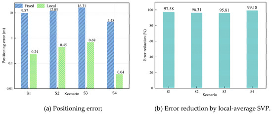
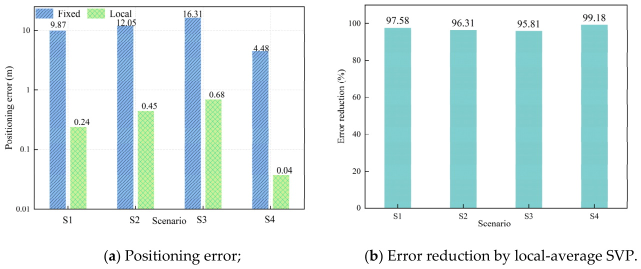
To evaluate the influence of different SVP modeling strategies on LBL localization results, baseline inversion is first performed using the constant-sound-speed model and the local average sound speed model. The results are shown in Figure 5. The constant-sound-speed model produces systematic localization bias in all four scenarios, with errors of 4.476–16.315 m. After introducing the local depth-weighted average sound speed, the errors decrease to 0.037–0.684 m. This confirms that vertical SVP non-uniformity is a major source of slant-range bias and that the source-depth sound speed alone is insufficient for high-precision localization.

Figure 5. Comparison of baseline localization errors under the constant sound speed and local average sound speed models.

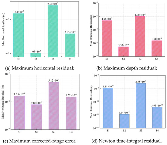
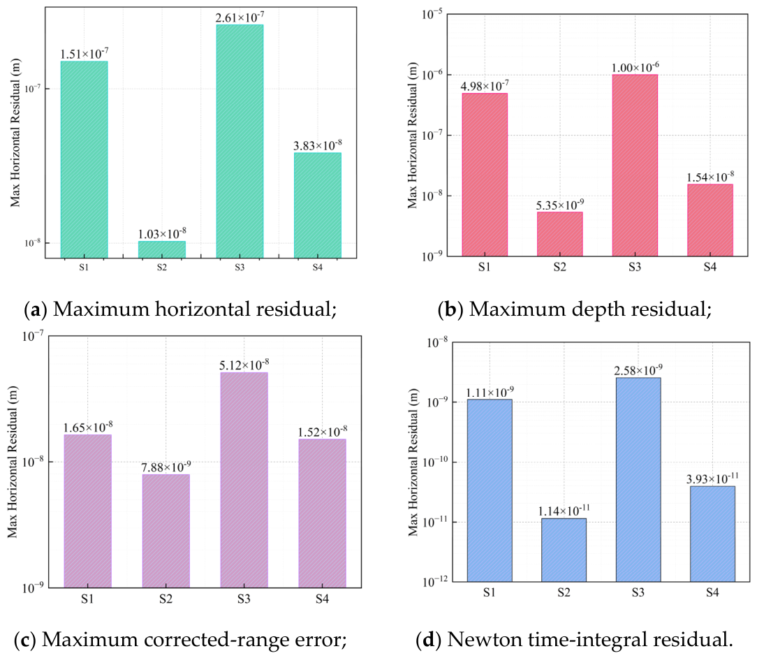
Before comparing localization performance, the numerical closure of the propagation-time-consistent ray inversion chain is further verified. As shown in Figure 6, under the TOA constraint, the ray parameters obtained by inversion are used for layered ray tracing. The endpoint horizontal residual, depth residual, and slant-range error are all at very low levels. Meanwhile, the time-integration residual of the Newton inversion is close to machine precision, confirming that the inverted parameters satisfy the propagation-time equation under the local SVP constraint. Thus, the TOA constraint, ray-parameter inversion, path tracing, and slant-range reconstruction form a numerically self-consistent chain for subsequent iterative localization correction. The very small residuals in this closure test should be interpreted as numerical consistency under idealized assumptions, rather than as practically achievable field localization accuracy. It should be noted that this closure test mainly verifies the numerical consistency of the forward and inverse ray-tracing chain. The very small residuals in this test should not be interpreted as field-achievable localization accuracy, but rather as an ideal consistency check before introducing observation noise, SVP mismatch, and measured-data inputs.

Figure 6. Numerical closure errors of the propagation-time-consistent ray inversion chain.

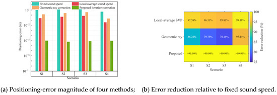
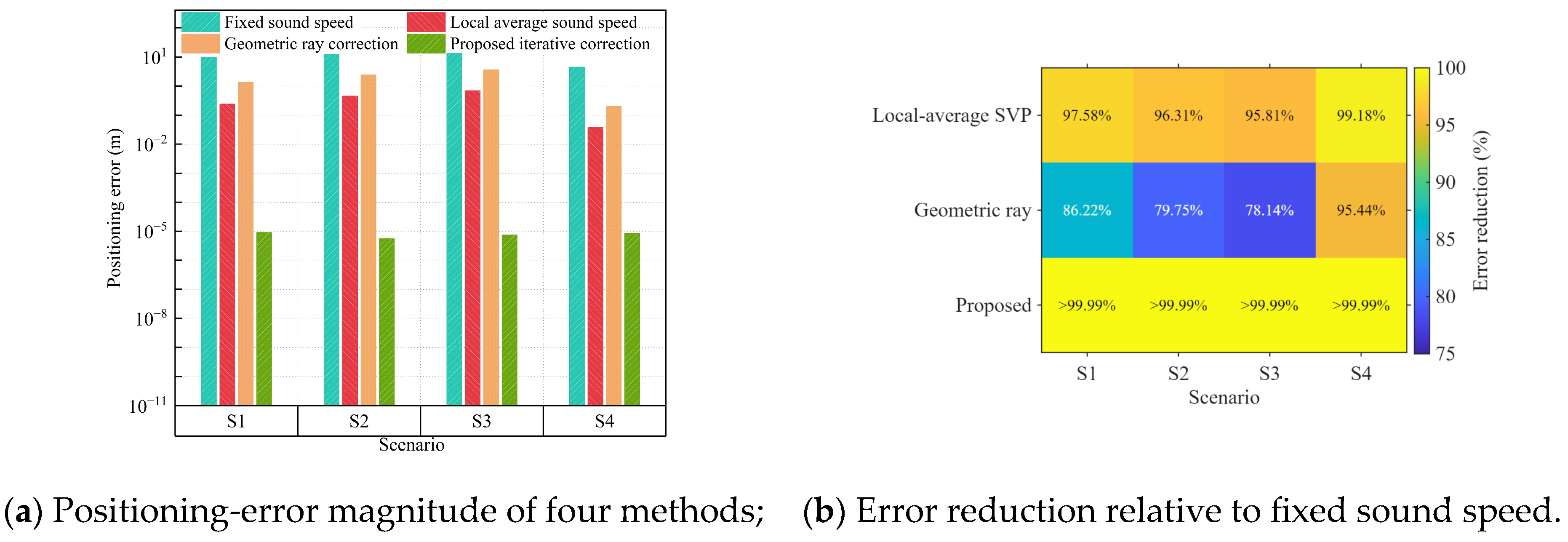
Figure 7 and Table 3 compare the four localization methods. The constant-sound-speed model produces clear bias in S1–S4, showing that propagation errors caused by non-uniform SVPs enter the localization solution. Although the local average sound speed and conventional geometric ray correction methods reduce the errors, they remain limited by equivalent-sound-speed approximation and one-time geometric compensation, respectively [16,19,22]. In contrast, under the ideal noise-free simulation setting, the proposed complete ray-path correction method achieves the lowest numerical residuals in all scenarios, with errors controlled at the order of 10⁻⁵ m. These results indicate the numerical consistency of the closed-loop correction chain rather than general field-achievable localization accuracy. Compared with equivalent-sound-speed or average-sound-speed models [15,16,19] and joint estimation methods for position and sound speed parameters [25,26], the proposed method realizes a lightweight closed-loop update through corrected-slant-range feedback.

Figure 7. Comparison of localization errors and error reduction rates under different SVP-based correction strategies.

Table 3. Error statistics of the four localization methods under different simulation scenarios.

Scenario	Constant Sound Speed/m	Local Average Sound Speed/m	Conventional Geometric Ray Correction/m	Proposed Method/m	Number of Outer Iterations
S1	9.872	0.239	1.360	9.06 × 10−6	20
S2	12.053	0.445	2.441	5.48 × 10−6	21
S3	16.315	0.684	3.567	7.39 × 10−6	21
S4	4.476	0.037	0.204	8.38 × 10−6	19

Note: The very small errors of the proposed method in Table 3 are obtained under ideal noise-free simulation conditions. They mainly indicate the numerical consistency of the propagation-time-constrained ray inversion and corrected-slant-range feedback chain and should not be interpreted as field-achievable localization accuracy.

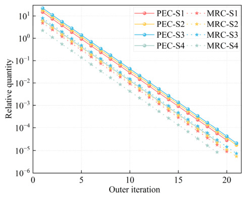
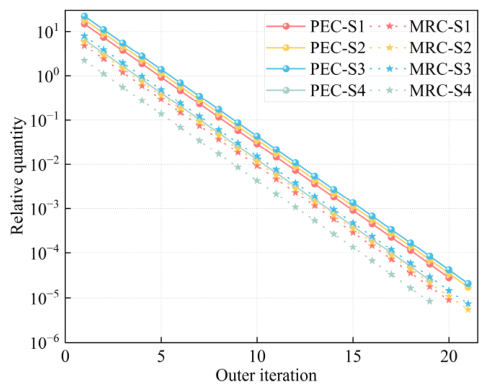
Figure 8 shows the joint convergence characteristics of the complete iterative ray-path correction method. The positioning error convergence (PEC) reflects the stability of the localization-layer position update, whereas the maximum range change (MRC) reflects the stability of the propagation-layer corrected-slant-range feedback. To allow comparison among scenarios with different initial errors and range scales, both quantities are expressed as relative values. In S1–S4, PEC and MRC decrease synchronously and converge after 20, 21, 21, and 19 outer iterations, respectively. This indicates that the corrected slant ranges and the WLS position estimates become stable in the same iterative process, confirming the closed-loop coupling between propagation correction and geometric localization.

Figure 8. Convergence characteristics of the complete iterative ray-path correction method proposed in this paper.

3.3. Stability Analysis Under Perturbed Conditions

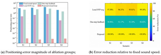
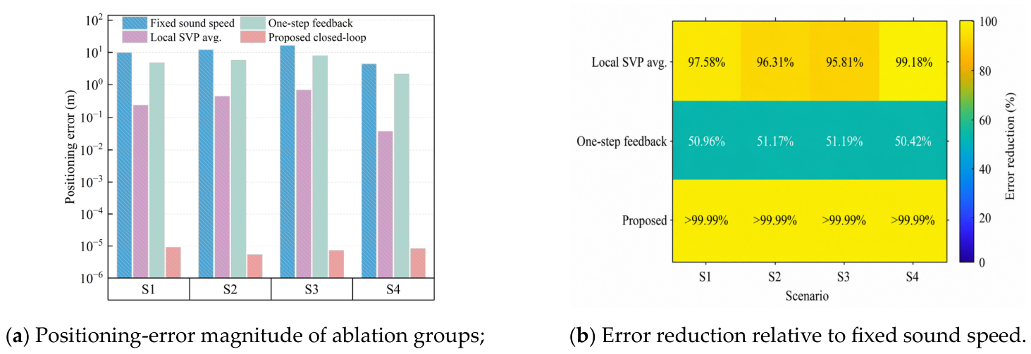
To avoid over-interpreting the noise-free simulations, the TOA-noise and SVP depth-shift tests are used to evaluate the method under observation uncertainty and propagation-model mismatch. To verify the role of the key modules, ablation experiments are conducted using four localization strategies: constant sound speed, path-dependent local average sound speed, conventional geometric ray correction, and the complete iterative method. As shown in Figure 9, the constant-sound-speed assumption produces meter- to tens-of-meter-level errors because the non-uniform SVP is not considered in the slant-range construction. The local average sound speed method reduces this bias by introducing path-dependent sound-speed information, but it still relies on an equivalent straight-line approximation. The conventional geometric ray correction method further considers ray bending, but its one-step correction does not fully suppress the transfer of slant-range errors to the position solution. By contrast, the complete iterative method combines TOA-constrained ray-parameter inversion, corrected-slant-range feedback, and WLS relocation, and therefore achieves the lowest errors in all four scenarios under the noise-free simulation setting.

Figure 9. Comparison of localization errors and error reduction rates in the ablation experiment of key modules.

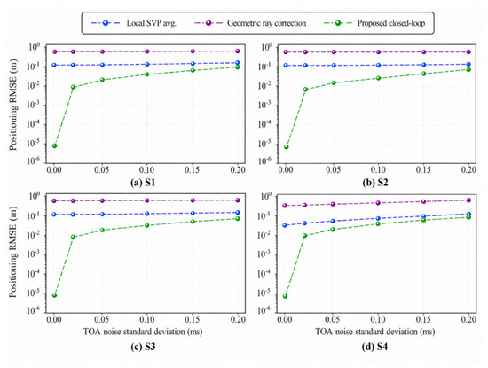
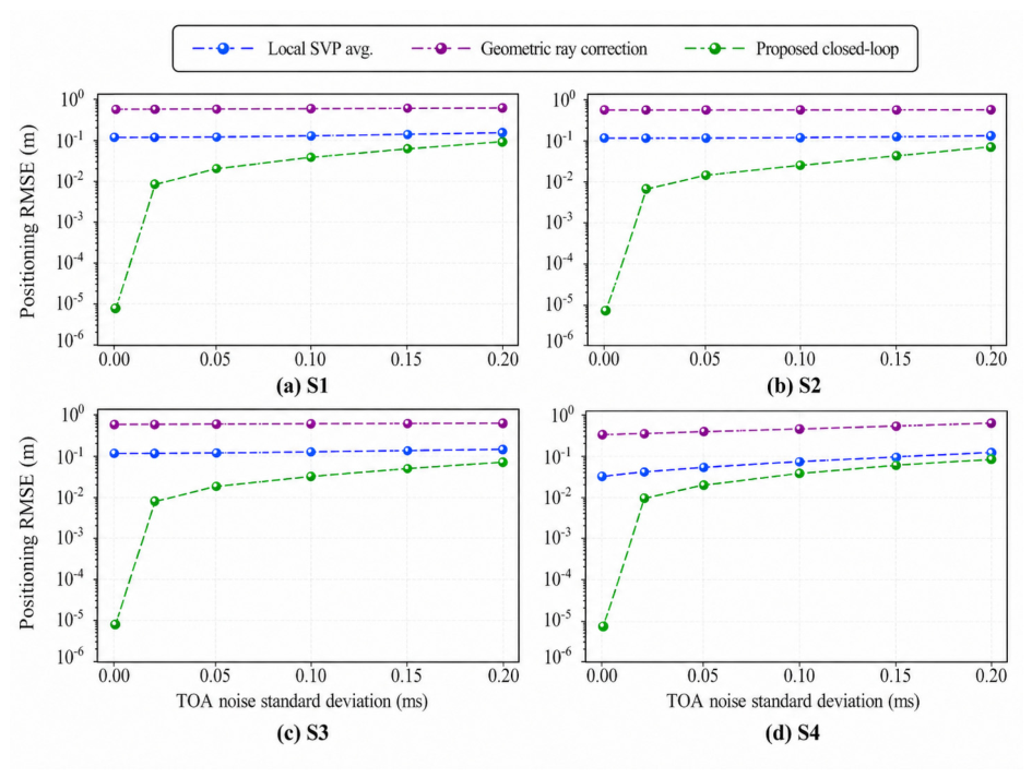
The reliability of TOA estimation directly affects the backend localization results. Related studies on TOA multi-feature fusion and time-difference-of-arrival localization have shown that timing errors are important factors affecting localization stability [38,39]. In this paper, Monte Carlo simulations are conducted under different standard deviations of TOA noise. As shown in Figure 10, the RMSE of all methods increases with TOA noise, but their relative error ranking remains generally stable. The proposed complete iterative method achieves the lowest RMSE in S1–S3 and performs close to the local average sound speed method in the weak-gradient scenario S4.

Figure 10. Comparison of localization RMSEs of SVP-based correction methods under different TOA noise levels.

Under the typical TOA noise level of 0.10 $\mathrm{ms}$, Table 4 further shows that the RMSE of the proposed method remains approximately 0.09–0.10 m in S1–S4. Compared with the constant-sound-speed model, the proposed method reduces the RMSE by 97.97–99.46%. Compared with the conventional geometric ray correction method, the reduction rate is 60.45–97.53%. These results show that the coupling between propagation-layer ray-path correction and localization-layer geometric solution helps improve localization stability under TOA noise conditions.

Table 4. Localization RMSEs of different methods and improvement rates of the proposed method under 0.10 $\mathrm{ms}$ TOA noise.

Scenario	Constant RMSE/m	Local RMSE/m	Geometric RMSE/m	Proposed RMSE/m	Red. vs. Constant/%	Red. vs. Local/%	Red. vs. Geometric%
S1	9.871	0.240	1.345	0.096	99.02	59.74	92.83
S2	12.059	0.446	2.434	0.095	99.21	78.73	96.10
S3	16.319	0.692	3.571	0.088	99.46	87.25	97.53
S4	4.471	0.100	0.229	0.091	97.97	9.51	60.45

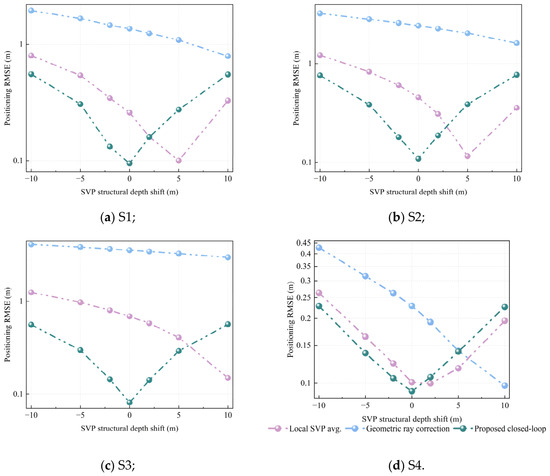
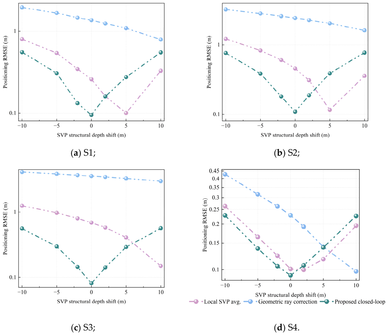
Under the 0.10 ms TOA-noise condition, SVP structural depth shifts from −5 m to 5 m are introduced to test method stability. As shown in Figure 11, the average RMSEs of the proposed method in S1–S4 are 0.197 m, 0.254 m, 0.195 m, and 0.120 m, respectively, and no error divergence occurs. The proposed method outperforms conventional geometric ray correction in all scenarios. Its advantage over the local-average-sound-speed method is clear in S1–S3, where SVP non-uniformity and ray bending are stronger, but becomes smaller in the weak-gradient scenario S4. These results indicate that the method remains stable under small SVP structural depth shifts, while its relative benefit depends on the degree of SVP non-uniformity.

Figure 11. Comparison of localization RMSEs of SVP-based correction methods under small SVP structural depth shifts.

Overall, the simulation results validate the proposed method in terms of localization accuracy, module contribution, and perturbation sensitivity. Local SVP modeling reduces constant-sound-speed bias, propagation-time-consistent inversion strengthens slant-range correction and corrected-slant-range feedback improves the consistency between propagation modeling and geometric localization. The SVP depth-shift test further examines a first-order layer-displacement mismatch, while more complex SVP uncertainties, such as depth-dependent bias, sparse sampling, local thermocline mismatch, and time-varying environmental changes, should be further evaluated with denser observations or additional sea-trial datasets.

4. Measured-Data Model Validation

4.1. Measured Data Sources and LBL Validation Scenario

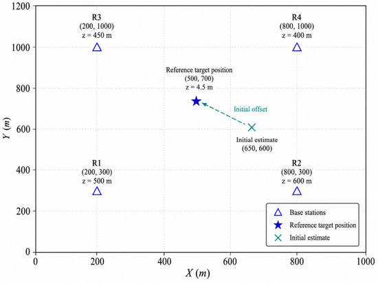
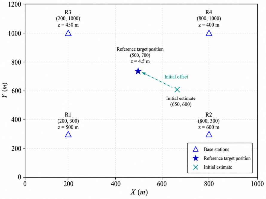
The validation data are from a sea trial in the Northern South China Sea. They include measured TOA inputs and a GDCSM-Argo observation-derived SVP. The SVP contains 58 depth layers. The depth range is 0–1975 m, and the sound speed range is 1482.723–1539.468 m/s. Figure 12 shows the measured-data validation scenario in the horizontal plane. A local Cartesian coordinate system is used, and the plotted coordinates represent only the planar geometry. The target reference position is [500, 700, 4.5] m, and the initial horizontal position is [650, 600] m. The four receiving base stations are located at [200, 300, 500] m, [800, 300, 600] m, [200, 1000, 450] m, and [800, 1000, 400] m, respectively. The depth coordinate (z) is measured positively downward from the sea surface. Since the target depth is known as 4.5 m, only the horizontal target position is estimated. To avoid ambiguity, the depth of each node is indicated in the figure labels rather than through the plotted coordinates.

Figure 12. Horizontal layout of the measured validation scenario.

This measured-data case is used as a representative validation scenario rather than an exhaustive robustness test. With real TOA inputs, an observation-derived multi-layer SVP, different receiver depths, and an in-network target, it provides a practical case for evaluating the proposed correction mechanism under realistic measurement and geometry conditions. Broader robustness should be further examined when more measured datasets become available.

The figure shows the planar distribution of the four LBL base stations, the reference target position, and the initial estimate. The depth of each node is indicated in the labels, while the plotted coordinates represent only the horizontal geometry.

To ensure the comparability of different SVP-based correction strategies, all methods use the same measured TOA data, observation-derived SVP, validation scenario coordinates, and WLS weights. The parameters for complete iteration, slant-range smoothing, and ray-parameter inversion in the proposed method are listed in Table 5.

Table 5. Main algorithm parameter settings in measured data validation.

Parameter	Value	Description
Maximum number of iterations $K_{\max }$	20	Outer-iteration limit
Slant-range smoothing factor $\alpha$	0.7	Slant-range smoothing
Slant-range convergence threshold ${\epsilon }_R$	0.01 m	Stopping criterion for range update
Newton iteration threshold ${\epsilon }_p$	1 × 10−5	Ray-parameter inversion tolerance
Initial WLS	Enabled	Constant-speed initial solution
Observation weight ${\omega }_i$	${\omega }_i$ = 1	Equal weights for all base stations

4.2. Validation of Localization Accuracy and Iterative Mechanism

To verify the applicability of the proposed method under measured-data input conditions, this section first compares the uncorrected constant-sound-speed method with the complete iterative ray-path correction method. This comparison evaluates the overall effect of ray-path correction on localization error suppression. Then, two baseline methods are introduced, namely local average sound speed correction and conventional geometric ray correction. They are used to analyze the performance difference between the proposed method and conventional correction strategies. Finally, an ablation comparison between single-step ray-path correction and complete iterative ray-path correction is conducted. Error convergence curves are also analyzed. These results reveal the roles of corrected-slant-range feedback and WLS localization updating.

4.2.1. Comparison Settings of the Four Strategies

In the measured-data validation scenario, four localization strategies are compared. The four methods use the same base-station deployment, target reference position, observation-derived SVP, measured TOA inputs, initial position, and WLS weights. They differ only in the slant-range construction method, ray-path correction method, and feedback mechanism.

The uncorrected constant-sound-speed method directly converts the two-way TOA into slant ranges using the sound speed near the target depth and serves as the straight-line baseline. The local average sound speed correction method constructs corrected slant ranges from path-specific local SVPs using depth-weighted average sound speed, representing an engineering approximation [15,16]. The conventional geometric ray correction method performs one-step layered ray-path correction based on the initial WLS geometry, representing a conventional ray-tracing compensation strategy [22,23,24]. This baseline uses the same SVP, TOA inputs, initial position, and WLS setting as the proposed method, but its ray correction is performed only once according to the initial geometric relationship, without TOA-consistency-constrained ray-parameter re-solving or corrected-slant-range feedback. In contrast, the complete iterative ray-path correction method solves the ray parameters through the propagation-time consistency equation. It then feeds the corrected slant ranges obtained by layered ray tracing back into the WLS localization model. This design is consistent with recent research trends in the coupled estimation of propagation parameters and position parameters [25,26]. However, this paper uses slant-range feedback to achieve a lightweight closed-loop update.

The above settings ensure that different methods are compared under the same measured TOA data, observation-derived SVP, and localization geometry. The constant-sound-speed method is used as the uncorrected baseline. The local average sound speed method and the conventional geometric ray correction method provide conventional correction baselines. The complete iterative ray-path correction method is used to verify the combined effects of the propagation-time consistency constraint, corrected-slant-range feedback, and WLS localization update.

4.2.2. Localization Results and Error Analysis

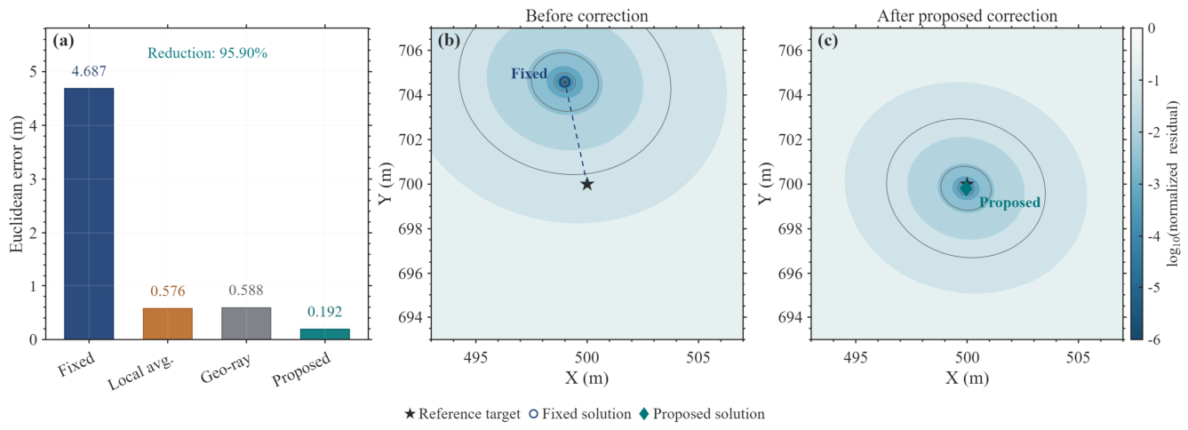
Table 6 presents the localization results of the four methods under measured TOA input conditions. The planar Euclidean error of the uncorrected constant-sound-speed method is 4.6866 m. After local average sound speed correction and conventional geometric ray correction, the errors decrease to 0.5757 m and 0.5880 m, respectively. This indicates that local SVP information can effectively reduce the slant-range bias caused by the constant-sound-speed assumption. However, residual errors still remain after single-step approximate compensation. Existing methods for time-varying SVP correction, in situ sound speed correction, and ESV table modeling have shown that the reasonable introduction of sound speed information can significantly reduce the systematic errors caused by the constant-sound-speed assumption [13,17,19]. The complete iterative method proposed in this paper further reduces the error to 0.1923 m. Compared with the two conventional correction methods, the error is reduced by 66.59% and 67.29%, respectively. Since the DOP values of the four methods are basically consistent, this result indicates that the accuracy improvement mainly comes from the propagation-time-consistent inversion and the corrected-slant-range feedback mechanism. It is not caused by changes in the base-station geometry.

Table 6. Localization results and error statistics under the four correction strategies.

Method	Final Position/m	X Error /m	Y Error /m	Euclidean Error/m	σ	DOP	Number of Outer Iterations	Improvement Relative to Uncorrected Method%
Constant sound speed, uncorrected	(498.9984, 704.5784)	−1.0016	4.5784	4.6866	8.514801	2.123326	0	0
Local average sound speed correction	(500.0121, 699.4244)	0.0121	−0.5756	0.5757	5.056554	2.124122	0	87.717
Conventional geometric ray correction	(500.0197, 699.4123)	0.0197	−0.5877	0.5880	5.067645	2.124124	0	87.454
Proposed iterative ray-path correction	(499.9486, 699.8147)	−0.0514	−0.1853	0.1923	0.518294	2.124062	18	95.896

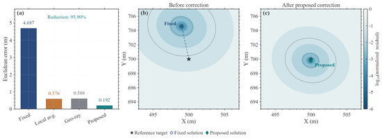
Figure 13 further visualizes the measured-data comparison using both localization errors and WLS residual maps. Panel (a) compares the Euclidean positioning errors of the fixed-sound-speed, local-average-SVP, geometric-ray-correction, and proposed methods. Panel (b) shows the normalized WLS residual objective map before correction, where the residual minimum corresponds to the fixed-sound-speed solution and is away from the reference target position. Panel (c) shows the residual map after the proposed correction, where the residual minimum is concentrated near the reference target position. The contour colors denote the log-scaled normalized residual objective, providing a spatial explanation for the improved localization accuracy of the proposed method.

Figure 13. Measured-data localization comparison and normalized WLS residual maps: (a) Euclidean positioning errors of different methods; (b) normalized WLS residual map before correction; (c) normalized WLS residual map after the proposed correction.

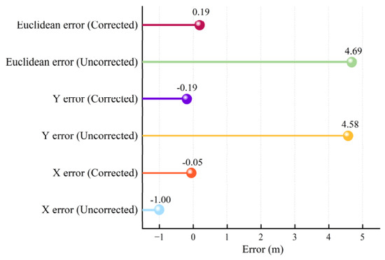
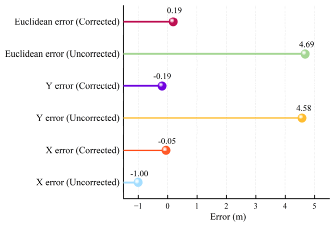
Figure 14 presents the error components before and after iterative correction. The uncorrected error is mainly concentrated in the Y direction, with a Y-direction error of 4.58 m. After correction, the X- and Y-direction errors decrease to −0.05 m and −0.19 m, respectively, and the planar Euclidean error decreases to 0.19 m, indicating effective suppression of the dominant directional bias caused by the constant-sound-speed assumption.

Figure 14. Comparison of localization error components before and after iterative ray-path correction.

4.2.3. Ablation Experiment and Iterative Convergence Analysis

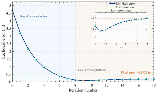
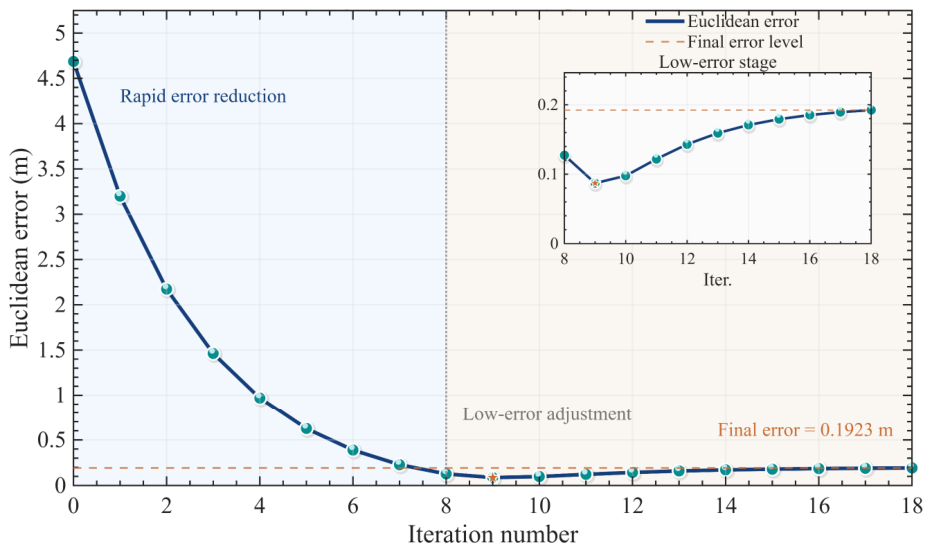
To further analyze the contribution of corrected-slant-range feedback and WLS localization updating, this paper uses single-step propagation-time-consistent ray-path correction as an ablation comparison. The single-step correction performs ray-parameter solving, layered ray tracing, and WLS localization updating only once. In contrast, the complete iterative correction continues to update the propagation geometry, ray parameters, and corrected slant ranges after each localization update until the convergence criterion is satisfied. The single-step correction reduces the planar Euclidean error from 4.6866 m to 3.1992 m, whereas the complete iterative correction further reduces it to 0.1923 m. This confirms the necessity of corrected-slant-range feedback and WLS localization updating. As shown in Figure 15, the error decreases rapidly in the early iterations and then fluctuates slightly within a low-error range before satisfying the slant-range convergence condition after 18 outer iterations. This behavior indicates an alternating coordination among propagation-path correction, slant-range updating, and WLS localization updating, rather than repeated optimization with fixed slant ranges.

Figure 15. Planar Euclidean error convergence curve during the iterative ray-path correction process and local enlargement of the low-error stage.

During the measured-data iterative process, $\Delta R_{\max }^{(k)}$ decreases from a maximum value of 3.042987 m to a minimum value of 0.007074 m, while $\Delta {\xi }^{(k)}$ decreases from 1.487756 m to 0.003303 m. These values indicate that both the corrected slant ranges and the horizontal position estimate gradually become stable during the outer iteration. The final $\Delta R_{\max }^{(k)}$ is lower than the convergence threshold of 0.01 m, which is consistent with the range-convergence stopping condition.

The algorithm-control parameters mainly affect convergence speed, stability, and computational cost. A larger smoothing factor improves update stability but may slow convergence, while a smaller value may accelerate feedback but increase oscillation under noisy TOA inputs. The maximum iteration number limits the outer loop, and the convergence threshold controls the trade-off between stopping precision and computational cost.

4.3. Stability and Perturbation Sensitivity Analysis

Existing studies have shown that SVP structure variations, propagation-time observation errors, and initial propagation geometry may all affect the stability of underwater acoustic localization [2,23,33,39]. Therefore, this paper further analyzes the local stability of the proposed method from three aspects: initial position, SVP modeling perturbation, and TOA input perturbation.

4.3.1. Sensitivity to SVP Modeling Bias

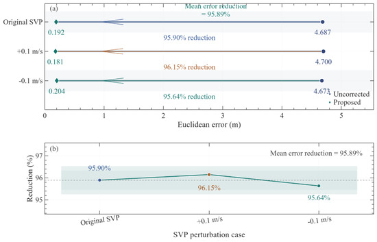
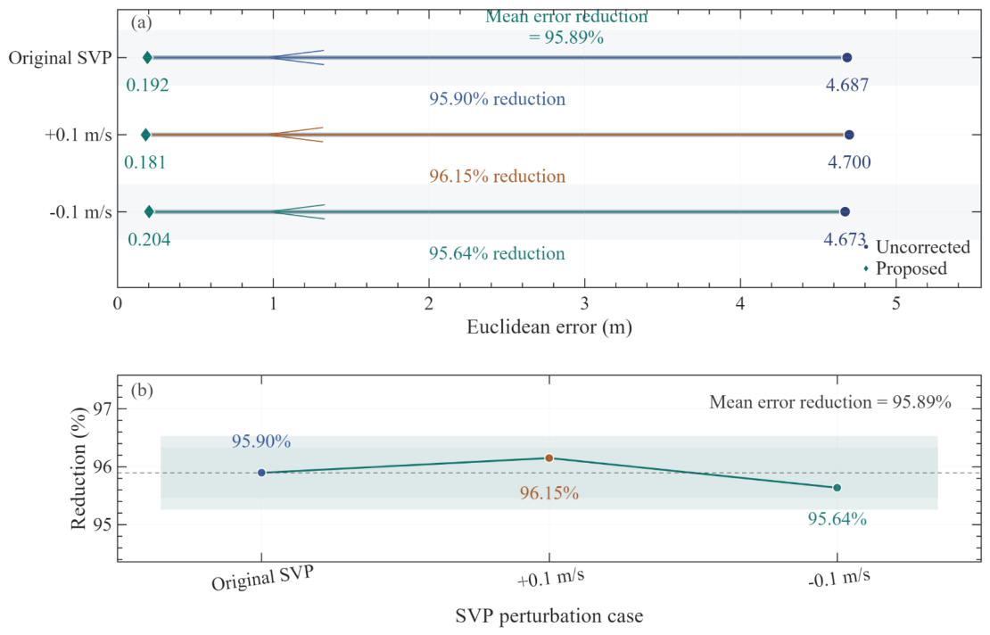
Since the proposed method uses the local SVP for propagation-time consistency and layered ray tracing, input SVP biases may affect ray-parameter inversion and corrected slant ranges. Similar effects have been reported in Global Navigation Satellite System–Acoustic (GNSS-A) and high-precision acoustic localization, where SVP errors enter the position solution through propagation-time interpretation [27,29,33]. To evaluate this local sensitivity, uniform sound speed biases of +0.1 m/s and −0.1 m/s are added to the observation-derived SVP, while the base-station positions, reference target position, and measured TOA inputs remain unchanged. The results are compared with those under the original SVP, without regenerating TOA observations.

Table 7 compares localization errors under different SVP input settings. For the original SVP, SVP +0.1 m/s, and SVP −0.1 m/s, the uncorrected method gives errors of approximately 4.7 m, whereas the complete iterative method gives 0.1923 m, 0.1809 m, and 0.2038 m, respectively. The corrected errors remain around 0.2 m, with reduction rates above 95%, an average error of approximately 0.192 m, and a standard deviation of 0.0115 m.

Table 7. Comparison of localization errors under small SVP perturbations.

SVP Setting	Method	X Error/m	Y Error/m	Euclidean Error/m	Improvement/%
Original SVP	Uncorrected	−1.0016	4.5784	4.6866	-
Original SVP	Iterative ray-path correction	−0.0514	−0.1853	0.1923	95.90
SVP +0.1 m/s	Uncorrected	−1.0031	4.5918	4.7001	-
SVP +0.1 m/s	Iterative ray-path correction	−0.0526	−0.1731	0.1809	96.15
SVP −0.1 m/s	Uncorrected	−1.0001	4.5649	4.6732	-
SVP −0.1 m/s	Iterative ray-path correction	−0.0503	−0.1976	0.2038	95.64

Figure 16 further shows that the proposed method maintains lower errors and stable reduction rates under the three SVP input settings. This test only considers small systematic SVP biases; therefore, it reflects the local sensitivity of the current measured-TOA LBL scenario rather than robustness to complex SVP uncertainties such as thermocline anomalies, sampling errors, or time-varying perturbations.

Figure 16. Comparison of localization errors and error reduction rates under different small SVP perturbations: (a) localization-error comparison before and after correction; (b) error-reduction rates under different SVP perturbation cases.

4.3.2. Sensitivity to TOA Observation Perturbations

Because the proposed method uses TOA observations to constrain ray-parameter inversion, TOA perturbations may propagate through corrected-slant-range construction and WLS localization. To evaluate this sensitivity, zero-mean Gaussian noise is added to the original two-way TOA observations, and Monte Carlo experiments are conducted under different perturbation levels. Let the original two-way TOA of base station $i$ be ${\tau }_i$. In the $q\text{-}th$ Monte Carlo experiment, the perturbed TOA is expressed as

$${\tau }_i^{(q)}={\tau }_i+\delta {\tau }_i^{(q)}$$

(25)

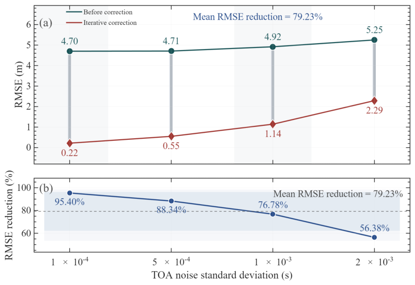
where $\delta {\tau }_i^{(q)}$ is a zero-mean Gaussian random perturbation. Four perturbation intensities are considered in this paper: 1 × 10⁻⁴ s, 5 × 10⁻⁴ s, 1 × 10⁻³ s, and 2 × 10⁻³ s. For each group, 100 Monte Carlo experiments are conducted. During the experiments, the target position, base-station geometry, and SVP input remain unchanged. Random perturbations are applied only to the two-way TOA input of the algorithm.

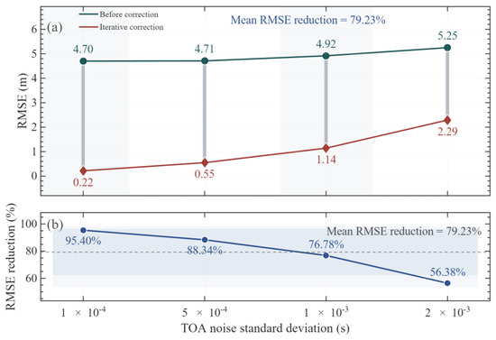
Table 8 shows that, as the TOA perturbation standard deviation increases from 1 × 10⁻⁴ s to 2 × 10⁻³ s, the RMSE of the uncorrected method increases from 4.7004 m to 5.2500 m. The RMSE of the iterative ray-path correction method increases from 0.2163 m to 2.2902 m. The corresponding RMSE reduction rate decreases from 95.40% to 56.38%. These results indicate that TOA input perturbations gradually weaken the ray-path correction effect. However, within the tested perturbation range, the iterative ray-path correction method still maintains better localization performance than the uncorrected method.

Table 8. Statistical results of the TOA small-perturbation sensitivity experiment.

TOA Perturbation Standard Deviation/s	Method	Mean Error/m	RMSE/m	Standard Deviation/m	Maximum Error/m	Average Number of Iterations	RMSE Reduction/%
1 × 10−4	Uncorrected	4.6995	4.7004	0.0757	4.9297	0	0
1 × 10−4	Iterative ray-path correction	0.2039	0.2163	0.0726	0.3978	18	95.40
5 × 10−4	Uncorrected	4.6958	4.7083	0.3451	5.4872	0	0
5 × 10−4	Iterative ray-path correction	0.4933	0.5488	0.2418	1.2763	18	88.34
1 × 10−3	Uncorrected	4.8532	4.9173	0.7956	7.0873	0	0
1 × 10−3	Iterative ray-path correction	0.9942	1.1416	0.5640	2.3069	18	76.78
2 × 10−3	Uncorrected	4.9776	5.2500	1.6774	9.7551	0	0
2 × 10−3	Iterative ray-path correction	2.0098	2.2902	1.1036	4.8429	18	56.38

Figure 17 further shows that the RMSE values of both methods increase as the TOA perturbation becomes stronger. This indicates that propagation-time errors are transferred to the localization solution through slant-range construction. In comparison, the iterative ray-path correction method always achieves a lower RMSE at all perturbation levels. The average RMSE reduction rate is approximately 79.23%. This indicates that the propagation-time consistency constraint and the corrected-slant-range feedback mechanism have a certain suppression effect on random TOA perturbations.

Figure 17. Comparison of RMSEs under different TOA perturbation intensities: (a) RMSE comparison before and after iterative correction; (b) RMSE reduction rate under different TOA perturbation intensities.

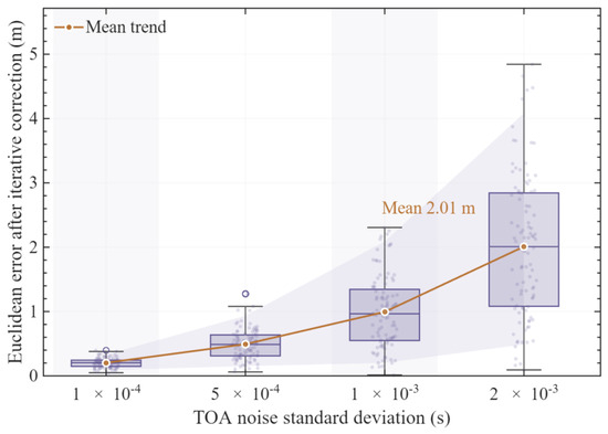
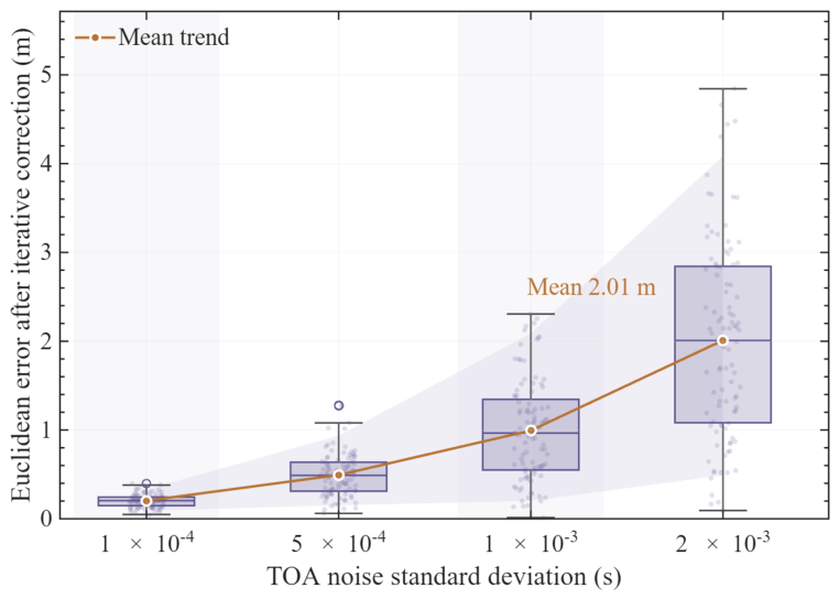
Figure 18 shows the error distribution of the iterative method. As the TOA perturbation increases, the median error, interquartile range, and sample spread all increase, confirming that the corrected results remain constrained by TOA input quality. Therefore, frontend signal enhancement methods, such as the generalized sidelobe canceller (GSC) [40], remain necessary, together with TOA confidence weighting.

Figure 18. Distribution of iterative correction errors under different TOA perturbation intensities. The boxplots show the median and interquartile range, the scattered points denote Monte Carlo samples, the orange line denotes the mean trend, the light-purple band indicates the 5th–95th percentile range, and the alternating light-gray background bands are used only to distinguish adjacent TOA perturbation levels.

Table 9 shows the trade-off between implementation simplicity and propagation-modeling consistency. The constant-sound-speed and local-average-sound-speed methods are easy to implement but have limited propagation-modeling capability, whereas the conventional geometric ray correction method considers ray bending but lacks TOA-consistency constraints and feedback updating. In comparison, the proposed method introduces higher computational complexity but forms a closed-loop update through propagation-time-consistent inversion, corrected-slant-range feedback, and WLS localization updating. In the measured-data scenario, it converges after 18 iterations and reduces the localization error to 0.1923 m.

Table 9. Comparison of computational complexity and engineering implementation characteristics of different SVP-based correction strategies.

Method	Local SVP	Ray- Parameter	Ray Tracing	Range Feedback	WLS	Iterations	Complexity	Engineering Characteristics
Constant sound speed, uncorrected	No	No	No	No	Single-step	0	Low	Simple; systematic range bias
Local average sound speed correction	Yes	No	No	No	Single-step	0	Low –medium	Local SVP; equivalent-speed approximation
Conventional geometric ray correction	Yes	Geometric initial value	Single-step	No	Single-step	1	Medium	Ray bending considered; no TOA feedback
Proposed closed-loop iterative ray-path correction	Yes	TOA constraint	Multi-step	Yes	Multi-step	18	Medium –high	Closed-loop update; improved accuracy

To further quantify this engineering complexity, the computational cost of the proposed method is analyzed. The dominant cost comes from TOA-constrained ray-parameter inversion and layer-wise ray tracing for each base station in each outer iteration. If $M$, $L$, $J$, and $K$ denote the number of base stations, average SVP layers, average Newton iterations, and outer iterations, respectively, the dominant complexity is approximately $O(KMJL)$. In the measured-data case, $M=4$, $L=33.25$ layers, $J=1.00$, and $K=18$. Tested on a 16-core AMD64 PC with 15.22 GB memory using MATLAB R2025b, the numerical localization core required approximately 4.0 ms per solution over 1000 repeated runs, excluding data loading, plotting, and file-output operations.

These findings are consistent with previous ESV- and average-sound-speed-based studies, in which sound-speed information is introduced to reduce the systematic bias caused by the constant-sound-speed assumption. Such methods are efficient and suitable when the SVP varies weakly, the target–receiver depth difference is small, or a single equivalent sound speed can reasonably represent the propagation path. The proposed method is expected to provide greater benefits under stronger vertical SVP gradients, larger target–receiver depth differences, longer propagation paths, and in-network geometries with acceptable observability, where equivalent-speed conversion may leave residual slant-range bias. Under weak SVP variation, poor TOA quality, or unfavorable sensor geometry, the improvement over local-average correction may become limited.

4.3.3. Discussion on Initialization, Geometry, and Practical Implementation

The robustness of the proposed method is affected by the initial seed and the target–sensor geometry. All simulation and measured-data cases in this study are conducted with the target located inside the sensor network. If the initial seed is outside the area enclosed by the sensors, the assumed propagation geometry may deviate from the actual target–sensor paths, which can increase range residuals, TOA-noise sensitivity, and iteration number, especially under strong sound-speed gradients or long-range propagation. In practice, the sensor-network centroid, previous-epoch solution, or auxiliary navigation information can be used to provide a more reliable initial seed.

When the target is outside the sensor network, the localization geometry changes from an interpolation-like to an extrapolation-like configuration. In this case, TOA errors, sensor-coordinate errors, and residual SVP uncertainties may be amplified in the final position [28,31]. Therefore, although the proposed ray-path correction can reduce SVP-induced systematic bias, it cannot fully compensate for geometric degradation caused by an unfavorable sensor layout. Increasing the sensor aperture, adding beacons, or incorporating motion/navigation constraints can help improve robustness in such cases.

Based on the above discussion, the factors that may reduce the efficiency of the proposed method can be grouped into five categories: TOA observation quality, SVP uncertainty, geometric observability, initialization and algorithm-control parameters, and computational scale. TOA noise, synchronization error, and multipath bias may disturb the propagation-time consistency constraint, while SVP bias, sparse sampling, layer displacement, and thermocline mismatch may affect corrected-slant-range construction. Poor DOP, nearly collinear source–receiver directions, or targets outside the sensor network may amplify WLS errors. In addition, unsuitable initial seeds, smoothing factors, iteration limits, or convergence thresholds may slow convergence, whereas the number of base stations, local SVP layers, and Newton iterations determines the main computational load. These factors should be considered jointly in practical deployment.

From a practical implementation perspective, the smallest TOA error considered in this study is 1 × 10⁻⁴ s, corresponding to a timing resolution of 0.1 ms and a range uncertainty of about 0.15 m for a nominal sound speed of 1500 m/s. A theoretical minimum sampling frequency of 10 kHz is, therefore, required, but this value only represents a lower bound because synchronization error, clock jitter, filtering delay, and correlation-peak estimation may also affect TOA accuracy. Typical sampling rates of 48–96 kHz provide time resolutions of about 20.8–10.4 μs, which are sufficient to support the TOA resolution used in this study when combined with correlation-based estimation and sub-sample interpolation [38]. Future work will further examine the influence of sampling rate, synchronization accuracy, and clock stability on positioning performance.

5. Conclusions

This paper proposes a propagation-time-consistent iterative ray-path correction method for known-depth two-dimensional LBL localization. By feeding TOA-consistent corrected slant ranges back into the WLS localization model, the method improves the coupling between propagation-path correction and geometric position updating. The known-depth assumption remains a practical constraint, because target-depth errors may affect local SVP extraction, ray-parameter inversion, corrected-slant-range construction, and the final WLS result. In the measured-data scenario, the planar Euclidean error decreases from 4.6866 m to 0.1923 m, corresponding to an error reduction rate of 95.90%. These results indicate that localization correction under non-uniform SVP conditions should jointly consider TOA interpretation, slant-range construction, and geometric localization updating.

Several limitations should be noted, and the conclusions of this study should, therefore, be interpreted within the tested simulation settings and the representative measured-data scenario. The method is formulated for known-depth two-dimensional LBL localization, and its performance may be affected by target-depth errors and TOA quality. The measured-data validation uses one representative sea-trial case with a specific receiver geometry, observed SVP, and measured TOA inputs, while the perturbation analysis mainly considers TOA noise and SVP structural depth shifts. Public release of the raw sea-trial data and complete code is restricted by laboratory confidentiality regulations and project data-management requirements, but a minimal synthetic benchmark and MATLAB implementation can be provided upon reasonable request. Broader validation under more diverse target depths, receiver layouts, SVP structures, and field environments will be conducted when additional qualified sea-trial datasets become available.

Future work may integrate ocean observation networks, underwater robotic clusters, and multi-source sensing platforms to extend static SVP correction toward time-varying environmental cognition and system-level cooperative localization.

References

- Li, T.; Zhao, J.; Ma, J. A Precise Underwater Positioning Method by Considering the Location Difference of Transmitting and Receiving Sound Waves. Ocean Eng. 2022, 247, 110480. [Google Scholar] [CrossRef] [Scilit]
- Thomson, D.; Dosso, S.E.; Gamroth, E.; Bradley, C. Modelling Uncertainty in an Underwater Acoustic Positioning System. Can. Acoust. 2012, 40, 13–18. Available online: https://jcaa.caa-aca.ca/index.php/jcaa/article/view/2501 (accessed on 7 June 2026).
- Huang, W.; Wu, P.; Lu, J.; Lu, J.; Xiu, Z.; Xu, Z.; Li, S.; Xu, T. Underwater SSP Measurement and Estimation: A Survey. J. Mar. Sci. Eng. 2024, 12, 2356. [Google Scholar] [CrossRef] [Scilit]
- Ming, W.; Sun, D.; Zhang, J.; Han, Y.; Tian, K. Research on High-Precision Long-Range Positioning Technology in the Deep Sea. J. Mar. Sci. Eng. 2025, 13, 1898. [Google Scholar] [CrossRef] [Scilit]
- Wu, Y.; Ta, X.; Xiao, R.; Wei, Y.; An, D.; Li, D. Survey of Underwater Robot Positioning Navigation. Appl. Ocean Res. 2019, 90, 101845. [Google Scholar] [CrossRef] [Scilit]
- Zhang, J.; Han, Y.; Zheng, C.; Sun, D. Underwater Target Localization Using Long Baseline Positioning System. Appl. Acoust. 2016, 111, 129–134. [Google Scholar] [CrossRef] [Scilit]
- Erbe, C.; Duncan, A.; Vigness-Raposa, K.J. Introduction to Sound Propagation Under Water. In Exploring Animal Behavior Through Sound: Volume 1: Methods; Erbe, C., Thomas, J.A., Eds.; Springer International Publishing: Cham, Switzerland, 2022; pp. 185–216. [Google Scholar]
- Porter, M.B. The BELLHOP Manual and User’s Guide: Preliminary Draft; Heat, Light, and Sound Research, Inc.: La Jolla, CA, USA, 2011; p. 70. [Google Scholar]
- Kang, Y.; Shen, X.; Yan, Y.; Wang, H.; Chang, J.; Liu, C. Sound Ray Correction Method for Deep-Sea Target Localization in Asynchronous Underwater Acoustic Sensor Networks. In Proceedings of the 2021 IEEE International Conference on Signal Processing, Communications and Computing (ICSPCC), Xi’an, China, 17–20 August 2021; IEEE: Piscataway, NJ, USA, 2021; pp. 1–5. [Google Scholar]
- Liu, Y.; Sun, Y.; Wang, X.; Tang, J.; Qi, H.; Zhang, T. An Adaptive Stratification Algorithm Based on Gradient Fitting Deviation and Its Application to Acoustic Ray-Tracing Algorithm. Ocean Eng. 2024, 311, 118809. [Google Scholar] [CrossRef] [Scilit]
- Xin, M.; Yang, F.; Wang, F.; Shi, B.; Zhang, K.; Liu, H. A TOA/AOA Underwater Acoustic Positioning System Based on the Equivalent Sound Speed. J. Navig. 2018, 71, 1431–1440. [Google Scholar] [CrossRef] [Scilit]
- Wang, J.; Xu, T.; Liu, Y.; Mu, D. Kalman Filter Based Acoustic Positioning of Deep Seafloor Datum Point with Two-Step Systematic Error Estimation. Appl. Ocean Res. 2021, 114, 102817. [Google Scholar] [CrossRef] [Scilit]
- Yu, M.; Cai, K.; Zheng, C.; Sun, D. Improvement of Seafloor Positioning Through Correction of Sound Speed Profile Temporal Variation. IEEE/CAA J. Autom. Sin. 2023, 10, 1099–1101. [Google Scholar] [CrossRef] [Scilit]
- Cheng, C.; Zheng, C.; Hong, X. A Deep-Sea Direct Sound Ranging Method Based on Effective Sound Velocity Estimation for Turning Ray. JASA Express Lett. 2025, 5, 066001. [Google Scholar] [CrossRef] [Scilit] [PubMed]
- Sun, D.; Li, H.; Zheng, C.; Li, X. Sound Velocity Correction Based on Effective Sound Velocity for Underwater Acoustic Positioning Systems. Appl. Acoust. 2019, 151, 55–62. [Google Scholar] [CrossRef] [Scilit]
- Liu, Y.; Lu, X.; Xue, S.; Wang, S. A New Underwater Positioning Model Based on Average Sound Speed. J. Navig. 2021, 74, 1009–1025. [Google Scholar] [CrossRef] [Scilit]
- Zhao, S.; Liu, H.; Xue, S.; Wang, Z.; Xiao, Z. Two-Step Correction Based on In-Situ Sound Speed Measurements for USBL Precise Real-Time Positioning. Remote Sens. 2023, 15, 5046. [Google Scholar] [CrossRef] [Scilit]
- Liu, T.; Duan, R.; Yang, K.; Su, B. Iterative Equivalent Sound Velocity Correction for Robust Localization in Long-Baseline Deep-Water Environments. Appl. Acoust. 2026, 241, 110961. [Google Scholar] [CrossRef] [Scilit]
- Xing, Y.; Wang, J.; Hou, B.; He, Z.; Zhou, X. Underwater Long Baseline Positioning Based on B-Spline Surface for Fitting Effective Sound Speed Table. J. Mar. Sci. Eng. 2024, 12, 1429. [Google Scholar] [CrossRef] [Scilit]
- Li, K.; Chitre, M. Data-Aided Underwater Acoustic Ray Propagation Modeling. IEEE J. Ocean. Eng. 2023, 48, 1127–1148. [Google Scholar] [CrossRef] [Scilit]
- Yokota, Y.; Ishikawa, T.; Watanabe, S.; Nakamura, Y.; Nagae, K. Representation and Interpretation about Underwater Sound Speed Gradient Field in the GNSS-A Observation. Geophys. J. Int. 2024, 237, 902–915. [Google Scholar] [CrossRef] [Scilit]
- Zhan, D.; Wang, S.; Cai, S.; Zheng, H.; Xu, W. Acoustic Localization with Multi-Layer Isogradient Sound Speed Profile Using TDOA and FDOA. Front. Inf. Technol. Electron. Eng. 2023, 24, 164–175. [Google Scholar] [CrossRef] [Scilit]
- Liu, Y.; Sanz Subirana, J.; Xu, T.; Wang, J.; Yang, W.; Zhang, S.; Shu, J. Ultra-Fast Calculation Method of Incident Angle Based on Underwater Acoustic Round-Trip Positioning. Ocean Eng. 2024, 305, 117998. [Google Scholar] [CrossRef] [Scilit]
- Liu, Y.; Xu, T.; Wang, J.; Li, M.; Mu, D.; Gao, Z. An Improved Method for Computing Acoustic Ray Incident Angle Based on Secant Method. Appl. Acoust. 2023, 205, 109293. [Google Scholar] [CrossRef] [Scilit]
- Sun, D.; Zhang, P.; Cai, K. Joint Estimation of Underwater Target Location and Sound Speed Profile Based on Argo Data. IEEE Internet Things J. 2025, 12, 17110–17122. [Google Scholar] [CrossRef] [Scilit]
- Liu, Y.; Wang, Y.; Chen, C.; Liu, C. Unified Underwater Acoustic Localization and Sound Speed Estimation for an Isogradient Sound Speed Profile. IEEE Sens. J. 2024, 24, 3317–3327. [Google Scholar] [CrossRef] [Scilit]
- Li, Z.; Dosso, S.E.; Sun, D. Joint Inversion for Transponder Localization and Sound-Speed Profile Temporal Variation in High-Precision Acoustic Surveys. J. Acoust. Soc. Am. 2016, 140, EL44–EL49. [Google Scholar] [CrossRef] [Scilit] [PubMed]
- Zhang, Y.; Li, Y.; Zhang, Y.; Jiang, T. Underwater Anchor-AUV Localization Geometries with an Isogradient Sound Speed Profile: A CRLB-Based Optimality Analysis. IEEE Trans. Wirel. Commun. 2018, 17, 8228–8238. [Google Scholar] [CrossRef] [Scilit]
- Watanabe, S.; Ishikawa, T.; Yokota, Y.; Nakamura, Y. GARPOS: Analysis Software for the GNSS-A Seafloor Positioning with Simultaneous Estimation of Sound Speed Structure. Front. Earth Sci. 2020, 8, 597532. [Google Scholar] [CrossRef] [Scilit]
- Tomita, F.; Kido, M. An Approximate Travel Time Calculation and a Robust GNSS-Acoustic Positioning Method Using an MCMC Technique. Earth Planets Space 2022, 74, 176. [Google Scholar] [CrossRef] [Scilit]
- Huang, W.; Wu, P.; Xu, T.; Zhang, H.; Meng, K. Optimal Reference Nodes Deployment for Positioning Seafloor Anchor Nodes in Internet of Underwater Things. IEEE Internet Things J. 2025, 12, 14254–14268. [Google Scholar] [CrossRef] [Scilit]
- Li, J.; Gu, Q.; Chen, Y.; Sun, G.; Huang, H. A Combined Ray Tracing Method for Improving the Precision of the USBL Positioning System in Smart Ocean. Sensors 2018, 18, 3586. [Google Scholar] [CrossRef] [Scilit] [PubMed]
- Yokota, Y.; Watanabe, S.; Ishikawa, T.; Nakamura, Y. Temporal Change of km-Scale Underwater Sound Speed Structure and GNSS-A Positioning Accuracy. Earth Space Sci. 2022, 9, e2022EA002224. [Google Scholar] [CrossRef] [Scilit]
- Liu, Y.; Xue, S.; Qu, G.; Lu, X.; Qi, K. Influence of the Ray Elevation Angle on Seafloor Positioning Precision in the Context of Acoustic Ray Tracing Algorithm. Appl. Ocean Res. 2020, 105, 102403. [Google Scholar] [CrossRef] [Scilit]
- Qiu, F.; Guo, D. Asynchronous Localization of Dynamic Node Through Underwater Acoustic Sensor Networks. Appl. Acoust. 2025, 228, 110275. [Google Scholar] [CrossRef] [Scilit]
- Huang, W.; Zhang, H.; Meng, K.; Gao, F.; Sun, W.; Shu, J.; Xu, T.; Li, D. Fast Ray-Tracing-Based Precise Underwater Acoustic Localization without Prior Acknowledgment of Target Depth. J. Mar. Sci. Eng. 2024, 12, 562. [Google Scholar] [CrossRef] [Scilit]
- Xin, M.; Yang, F.; Xue, S.; Wang, Z.; Han, Y. A Constant Gradient Sound Ray Tracing Underwater Positioning Algorithm Considering Incident Beam Angle. Acta Geod. Cartogr. Sin. 2020, 49, 1535–1542. [Google Scholar]
- Ma, C.; Wang, L.; Gao, J.; Cui, Y.; Peng, C.; Zhang, S. Time of Arrival Estimation for Underwater Acoustic Signal Using Multi-Feature Fusion. Appl. Acoust. 2023, 211, 109475. [Google Scholar] [CrossRef] [Scilit]
- Mandić, F.; Mišković, N.; Lončar, I. Underwater Acoustic Source Seeking Using Time-Difference-of-Arrival Measurements. IEEE J. Ocean. Eng. 2020, 45, 759–771. [Google Scholar]
- Cohen, I. Analysis of Two-Channel Generalized Sidelobe Canceller (GSC) with Post-Filtering. IEEE Trans. Speech Audio Process. 2003, 11, 684–699. [Google Scholar] [CrossRef] [Scilit]
Disclaimer/Publisher’s Note: The statements, opinions and data contained in all publications are solely those of the individual author(s) and contributor(s) and not of MDPI and/or the editor(s). MDPI and/or the editor(s) disclaim responsibility for any injury to people or property resulting from any ideas, methods, instructions or products referred to in the content. |
© 2026 by the authors. Licensee MDPI, Basel, Switzerland. This article is an open access article distributed under the terms and conditions of the Creative Commons Attribution (CC BY) license.