Assessment of Wave Energy Converter Performance with Satellite Data

Abstract

Recent advances in satellite measurements make satellites suitable candidates for monitoring the ocean environment, especially in the case of offshore wave resources. In this context, the present work aims to evaluate the accuracy of the wave dataset provided by the European Space Agency’s Sea State Climate Change Initiative (or CCI-SS) project, in order to establish its viability to be used for renewable energy applications in general and those associated with some European locations in particular. Seventeen years of ERA5 data (2002–2018) are also considered for comparison with the satellite measurements. The first step is to derive the wave periods corresponding to the significant wave heights provided by the satellite from the ERA5 data by establishing a quadratic relationship between the significant wave height (Hs) and the wave period (Te). As a next step, the local wave conditions are expressed in terms of wave power distribution, also considering the performance of three wave energy generators with nominal power ranging from 250 to 3619 kW. By comparing with ERA5 data, it was observed that the CCI-SS dataset generally overestimates the wave energy for the sites located in the oceanic environment, also indicating much higher values for the converters with a rated power that does not exceed 1000 kW.

1. Introduction

Oceans cover nearly 70% of the Earth’s surface, and they are considered very dynamic environments that influence weather patterns, support life forms, and are increasingly recognized as a major source of energy. Since the early days, people have tried to collect ocean information from a variety of in situ sources, such as buoys, sonars, or tide gauges [1]. The rapid evolution of computational systems has drawn attention to some new approaches for predicting and monitoring sea state conditions over large areas of water. One of the most commonly used approaches is related to numerical simulations, which can be tuned for different accuracy levels or purposes, such as prediction of the sea state from a climatological point of view. It is essential to note that the precision of the numerical models is significantly affected by the quality of the input data, and usually this involves an assimilation process, in which a satisfactory equilibrium can be expected between the real-world conditions and the spatial/temporal resolution. This is typically achieved by aggregating knowledge from prior initiatives, as exemplified by the ERA5 dataset, which is a continuation of the ERA-Interim study [2,3].

In recent decades, remote sensing platforms have progressively integrated into the landscape, and they are currently regarded as one of the most dependable sources of marine data. TIROS-1 is considered to be the inaugural successful weather satellite, launched on 1 April 1960, by NASA (National Aeronautics and Space Administration). Despite its operation lasting just 78 days, this mission generated about 19,000 photos of Earth’s surface weather, encompassing visuals of cloud clusters and tropical cyclones [4]. This breakthrough significantly advanced weather monitoring, enabling the development of similar platforms capable of measuring various atmospheric and terrestrial characteristics.

The launch of METEOSAT-1 in Europe in December 1977 marks another significant milestone, since this was the first European geostationary meteorological satellite. The initiative, begun by France in the early 1970s, required the inclusion of additional partners, such as Belgium and Germany, in 1975 to accelerate the project implementation. The results were presented as Earth imagery and data for various meteorological products, including solar radiation, cloud cover, air humidity, sea and land surface temperature, cloud temperature, and wind vectors [5,6].

The advantages of using a geostationary satellite are evident, as a single mission can cover nearly 40% of the Earth’s surface, and the resultant data can be employed for diverse research areas, including climate change effects, operational meteorology, search and rescue operations, environmental monitoring, and renewable applications. At this moment, in addition to Europe and the U.S., some other countries are using satellites, including Japan, India, China, Russia, and South Korea [7].

As expected, the significance of satellite measurements in the marine renewable industry is substantial, as these data are used for evaluating natural resources and predicting various offshore systems, such as wind turbines. A comprehensive analysis typically incorporates supplementary data sources, such as in situ measurements or numerical models, alongside the application of machine learning [8,9]. This is the case of Rusu and Rusu (2021), in which a comprehensive analysis of wave energy was conducted based on altimeter measurements and ERA5 data [10]. A total of 27 years (1992–2018) of satellite data were considered, and the results indicated good agreement between satellite and reanalysis data.

Other studies use satellite observations in order to improve the performance of numerical wave models for the Black Sea [11], the Indian Ocean [12], China’s coastal seas [13], or the North Atlantic [14]. These studies reveal that a limitation of satellite measurements is that they provide especially significant wave heights (Hs), therefore lacking information on wave periods. This is not the case for offshore wind, which can be by throughout satellite imagery [15,16]. Synthetic Aperture Radar (SAR) is frequently used to assess the wind flow over areas of large offshore wind projects, like those in the North Sea [17,18]. However, in recent years, other wave parameters have also been retrieved from SAR (such as the average wave period), with good accuracy [19].

By reviewing the existing literature, we can notice that a significant part of the research is dedicated to the joint analysis of wave height and wind speed, covering in particular the agreement between satellite measurements and some well-established data sources. Some studies provide a general analysis on a global scale [20,21,22], while other research covers, in more detail, some specific environments, such as the Marmara Sea [23], the Mediterranean Sea [24], Europe [25], or Ireland [26]. Other topics include coastal protection, as in the case of Giglio Island (Mediterranean Sea), where several generic wave farms were considered for evaluation [27]. The satellite measurements were reprocessed within the framework of the European Space Agency’s (ESA) Sea State Climate Change Initiative (CCI-SS) project using new algorithms to enhance measurement accuracy (with a particular focus on the coastal zone [28]) and to determine the extreme sea state [29].

As mentioned, a limitation of altimeter measurements is the lack of wave period values. Numerous approaches have been proposed to address this problem, such as the use of empirical models that take into account satellite wind speed data, geometrical optics approximations, or correlation with buoy measurements. In the work of Gommenginger et al. [30], several empirical models were constructed in order to predict the values of peak (T_p), mean (T_m), and zero-crossing wave periods (T_z). A correlation between the wave period and the significant wave height could be established through the use of a quadratic regression. The collocation of the Topex/in situ dataset highlights the fact that a straightforward empirical model may replicate a wide range of wave periods. Wang and Ichikawa [31] highlighted that the altimeter measurements are susceptible to high-frequency waves and that low-wind conditions may result in notable variations. Since a buoy system cannot record waves shorter than its dimension, it is important to adjust for these events in order to achieve agreement between satellite and buoy data, hence neglecting high-frequency components.

In this context, the objectives of the current work are to

(a)

Derive the wave period of the CCI-SS project data (version 4) for several European locations from the correlation between the ERA5 dataset and the satellite measurements;

(b)

Compare the wave period, wave height, and wave energy directly between the satellite and ERA5 data;

(c)

Evaluate the performance of several wave energy converters using the satellite observations.

2. Materials and Methods

2.1. Target Area

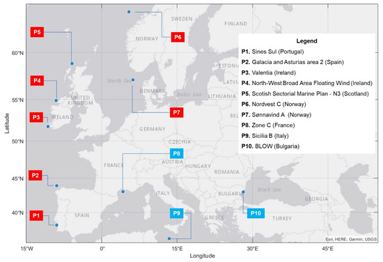
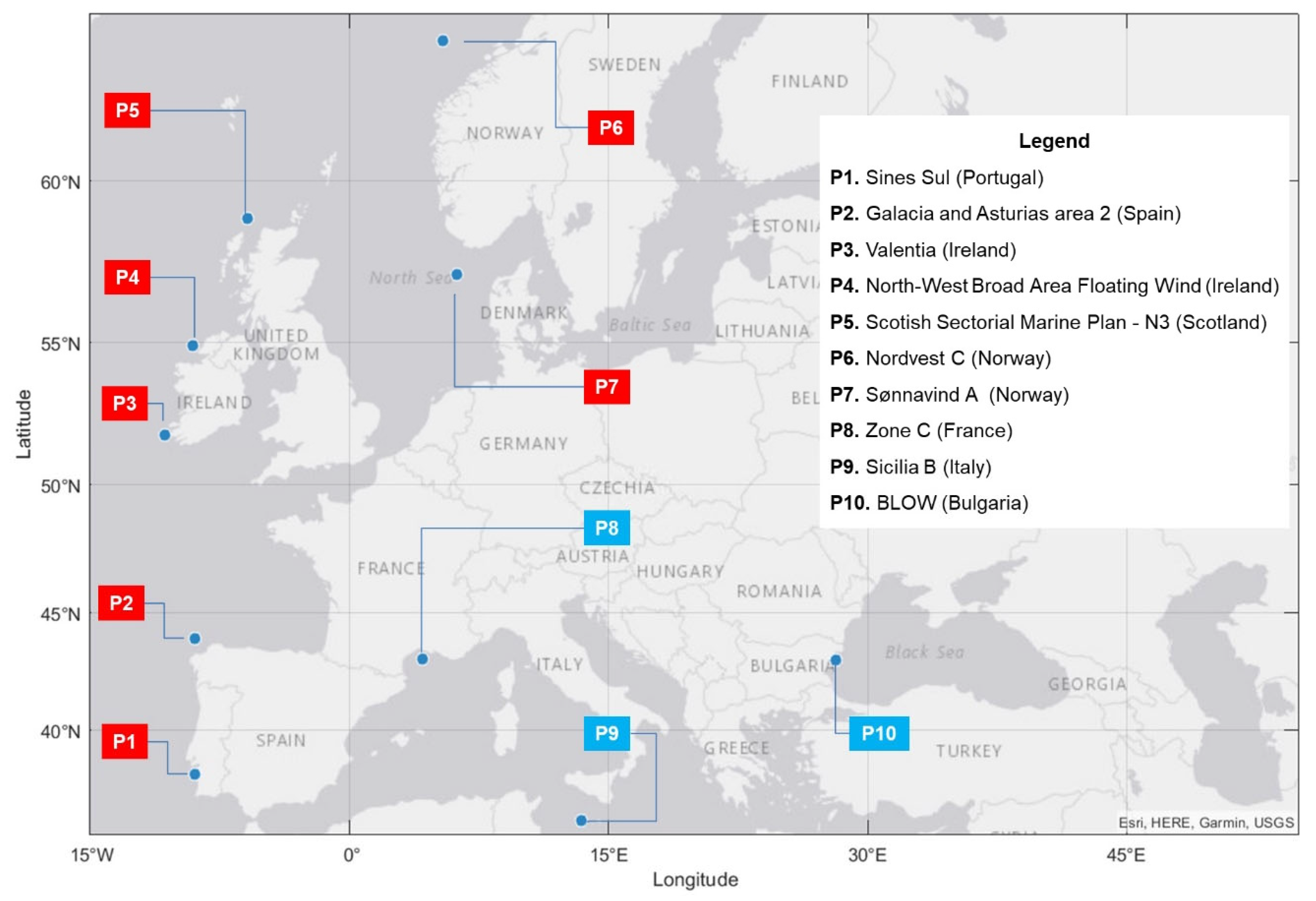
The locations of the ten European reference points (denoted from P1 to P10) considered for evaluation are illustrated in Figure 1, while Table 1 provides some additional information, such as the coordinates or distance from the coast. These locations were chosen based on their capacity to host marine renewable projects, covering all the major water areas (such as the ocean and enclosed seas). As can be seen, the majority of them are built to accommodate offshore wind projects, which will serve as an appropriate foundation for the deployment of wave energy converters.

Figure 1. The European sites considered for assessment, where: (a) red color—sites located near the ocean or open seas; (b) blue color—sites located on enclosed basins.

Table 1. Technical details of the European marine sites.

Site	Name	Country	Details	Lat (°)	Lon (°)	Water Depth (m)	Distance to Shore (km)
P1	Sines Sul	Portugal	Development zone	38.02	−9.00	171	14
P2	Galacia and Asturias Area 2	Spain	Floating wind	43.95	−9.00	2350	65
P3	Valentia	Ireland	Floating wind	51.82	−10.74	38	21
P4	North-West Broad Area Floating Wind	Ireland	Floating wind	54.90	−9.11	78	30
P5	Scottish Sectorial Marien Plan	Scotland	Development zone	58.89	−5.92	96	61
P6	Sønnavind A	Norway	Development zone (wind)	63.80	5.40	690	123
P7	Nordvest C	Norway	Development zone	57.17	6.20	61	105
P8	Zone C	France	Development zone	43.11	4.22	89	40
P9	Sicilia B	Italy	Floating wind	35.92	13.40	636	141
P10	BLOW	Bulgaria	Floating wind	43.04	28.19	30	23

The concept of hybrid wind-wave farms has gained attention in recent years as a potential solution to the expensive development of a marine project and a more reliable energy output that will be less influenced by the intermittent nature of wind and wave resources [32,33,34].

The first five sites (P1–P5) are located in coastal areas with consistent wave energy resources, followed by sites that are more relevant for offshore wind development. This is the case of site P10, where a 5-MW demonstrator floating offshore project will be developed within the context of the BLOW (Black Sea Floating Offshore Wind) project [35].

The primary goal of this work is to demonstrate the ability of CCI-SS altimeter data to be used for evaluating a specific sea state from the perspective of renewable energy resources. Satellite measurements are already known to have specific uncertainties in coastal areas (land contamination), with some studies indicating that the accuracy can be lower up to 10 km from the coast [36,37]. None of the selected locations are within this range; the nearest point selected is P1 (Sines Sul, Portugal), while P9 (Sicilia B, Italy) has the maximum distance of 141 km.

However, substantial advances have been achieved in coastal altimetry in recent years. Notably, dedicated retracking algorithms have been developed to minimize the influence of spurious reflections from nearby coastal features, which can otherwise compromise the parameter estimation [38,39]. Combined with robust outlier detection procedures, these developments have considerably enhanced both the accuracy and the availability of significant wave height measurements.

2.2. Datasets and Methodology

The satellite observations retrieved from the Climate Change Initiative for Sea State (CCI-SS version 4, https://cciseastate.gitlab-pages.ifremer.fr/ccidoc/access.html, accessed on 11 April 2026) project represent the first database used in this investigation [40]. This is regarded as a multi-mission effort in which multiple space-borne radar altimeters are combined to produce a uniform collection of data from 1991 to present. The historical missions include ERS-1, TOPEX, and ENVISAT, while the operational missions include CRYOSAT-2, SARAL, and JASON-3. The majority of measurements are conducted in the Ku band by satellites with a repeat period of 10–35 days, except for CRYOSAT-2, which follows a 369-day orbit. The operational altitude of this altimeter is categorized into two segments: (a) 717–800 km and (b) 1336 km, with an instrument inclination ranging from 66° to 108° [40]. The CCI-SS dataset (version 4) used in this study includes measurements of significant wave height (Hs), of which the Level 4 product provides global gridded Hs. These values represent monthly multi-mission data (one value per month), combined from all the existing altimeter missions, with a spatial resolution of 1° × 1°, as used also in [10]. For the current study, time series of the Hs parameter for each reference site (P1–P10) were extracted, representing average values (one value per month) for the years 2002–2018. ERA5, which is characterized by global coverage and constant spatial/time resolution, is the other database considered in this work. It was chosen since it is commonly used as a reference in climate, meteorological, and renewable energy studies [3]. Two wave parameters, Hs and the energy mean wave period (Te), also referred as the mean wave period, were processed for the current study [41]. These parameters, which are defined by eight values per day (00-03-06-09-12-15-18-21 UTC), were processed to cover the same time interval as the satellite data (CCI-SS, 2002–2018). However, the ERA5 data were averaged to obtain a monthly value in order to directly compare the two datasets. It is worth pointing out that the two datasets have already been compared globally, and the results show, in general, that there is good agreement between them, with some differences observed near the Arabian Sea and the Indian Ocean [10].

As mentioned, the selected sites are associated with deep-water areas (except for P10), which means that it is possible to use the linear wave theory for deep-water waves. The deep-water wavelength L₀ scales quadratically with the wave period, as follows [42]:

$$L_0={\displaystyle \frac{g{T}^2}{2\pi }}$$

(1)

where g is the gravity acceleration, and T is the wave period. The steepness of a deep-water wave relates the height H to the wavelength L₀. The maximum wave height before it breaks is limited by the maximum steepness. In deep water, the limiting wave steepness ratio is expressed as [42]

$${\displaystyle \frac{H}{L_0}}\approx 0.14$$

(2)

This means that the physical limit gives a quadratic relation between the wave height and period when waves approach their maximum breaking limit. Substituting the deep-water wavelength L₀ into Equation (2) yields a quadratic relation for the maximum wave height [42]:

$$H=0.14\left({\displaystyle \frac{g{T}^2}{2\pi }}\right)$$

(3)

Based on these theoretical aspects, a quadratic polynomial function will be used to establish a possible relation between the wave height and period of the ERA5 data. This will be done for each site, and the results will be further used to estimate the wave period of the satellite data, starting from the given Hs values.

Based on the deep-water wave theory, it was established that a quadratic relation could be used to make a connection between the parameters Hs and Te of the ERA5 dataset. This was done in the MATLAB R2026a environment by using the coefficients for a polynomial p(x) of the second degree that is a best fit (in a least-squares sense) for the data in y. This can be expressed as [43]

$$p(x)=p_1{x}^2+p_{2}x+p_3$$

(4)

In addition to evaluation of Hs and Te, a complete picture of the wave energy resources can be obtained by considering the mean wave power density (or Pw), which is defined as [44]

$$P_w={\displaystyle \frac{\rho g^2}{64\pi }}{T}_e{H}_s^2$$

(5)

where P_w (kW/m) is the energy flux per meter, $\rho$ = 1025 kg/m³ represents the seawater density, and g is the gravitational acceleration (9.81 m/s²).

The performance of a given wave energy converter (WEC) is obtained by combining the power matrix of a wave generator with the bivariate distribution of the sea state (ex: Hs × Te) of a particular site. This is indicated as [44]

$$P_E={\displaystyle \frac{1}{100}}\cdot {\displaystyle \sum _{i=1}^{nT}{\displaystyle \sum _{j=1}^{nH}P{W}_{ij}}}\cdot P{M}_{ij}$$

(6)

where PW_ij is the bivariate distribution of the bin defined by line i and column j, and PM_ij is the expected bin power output associated with the power matrix of a particular WEC (same i and j combination). The power matrices are provided by the developers of these systems, some of which are well-known and often used in this type of research, with the mention that new WECs are continually designed as the wave technology advances [41,44].

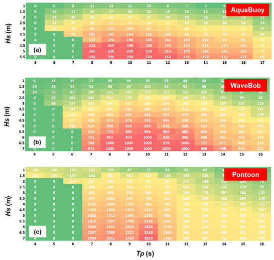
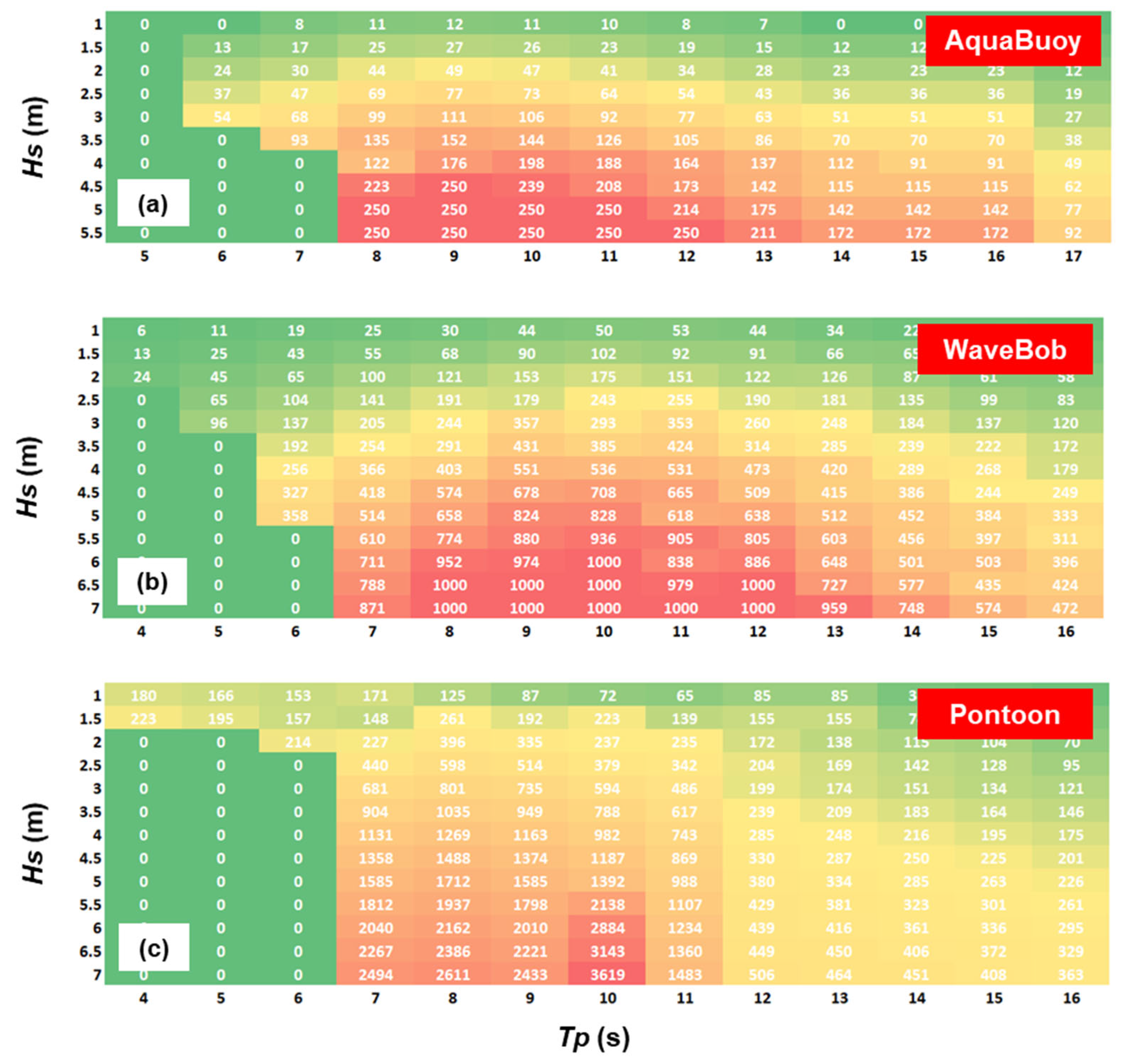
Figure 2 presents the power matrices of three WECs, which were selected based on their capability to operate in deep-water areas. All of them are classified as point absorbers, being defined by the following rated powers: AquaBuoy—250 kW; WaveBob—1000 kW; Pontoon—3619 kW. It can be seen from the x-axis of the power matrices that there are wave generators for which the designers indicate their performance in terms of the peak period (Tp). The following correspondence is used to establish a correlation between the Tp and Te, which is valid for a deep-water environment [45]:

$$T_e=0.9\cdot T_p$$

(7)

Figure 2. Wave energy converter power matrices. (a) AquaBuoy; (b) WaveBob; (c) Pontoon. Information processed from [46].

3. Results

As already mentioned, the altimeter data do not provide measurements along the tracks in terms of the wave period. In order to estimate a quadratic regression, defined by particular coefficients, it is possible to use the ERA5 data to establish the best fits between the parameters Hs and Te. The specific trend equations estimated for each site, considering ERA5 data (monthly values), are presented in Table 2. These relationships are further used to obtain the Te parameters related to the CCI-SS project by using as input the Hs parameters associated with the satellite measurements.

Table 2. The best fits between the Te and Hs parameters related to the ERA5 dataset’s quadratic trend line (monthly values). The results are processed taking into account all the reference sites for the entire time period (2002–2018), and also the main statistical parameters (SSE, R², and RMSE).

Site	Trend Line Equation	Statistic
		SSE	R2	RMSE
P1	Te = (−0.9991)Hs2 + (6.3183)Hs + 0.9941	96.07	0.77	0.69
P2	Te = (−0.2541)Hs2 + (2.8454)Hs + 3.2654	51.11	0.83	0.50
P3	Te = (−0.2041)Hs2 + (2.3397)Hs + 4.0720	39.55	0.84	0.44
P4	Te = (−0.2465)Hs2 + (2.6019)Hs + 3.8035	43.81	0.84	0.46
P5	Te = (−0.2039)Hs2 + (2.2643)Hs + 3.9817	25.95	0.88	0.35
P6	Te = (−0.2439)Hs2 + (2.4321)Hs + 3.8295	36.28	0.84	0.42
P7	Te = (−0.2283)Hs2 + (2.1343)Hs + 3.0744	18.06	0.84	0.29
P8	Te = (−0.6753)Hs2 + (2.8979)Hs + 2.1256	7.13	0.85	0.18
P9	Te = (−0.5887)Hs2 + (2.9867)Hs + 2.4058	3.59	0.95	0.13
P10	Te = (−0.9171)Hs2 + (3.3742)Hs + 2.1514	3.87	0.90	0.13

From a statistical point of view, the accuracy of a polynomial quadratic approach can be defined by using the SSE (sum of squares due to error), R², and RMSE (Root Mean Square Error) indicators. For example, in the case of the SSE and RMSE indicators, a perfect correlation is associated with zero, while for R² a value located close to 1 is considered to be ideal [47]. From this point of view, better performances are expected for the sites from the Mediterranean and Black Sea (RMSE = 0.13), while on the opposite side we can find site P1 with an RMSE value of 0.69. Sites P2–P6 are defined by RMSE values located in the range of 0.35 and 0.5.

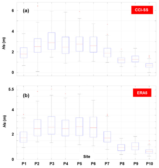
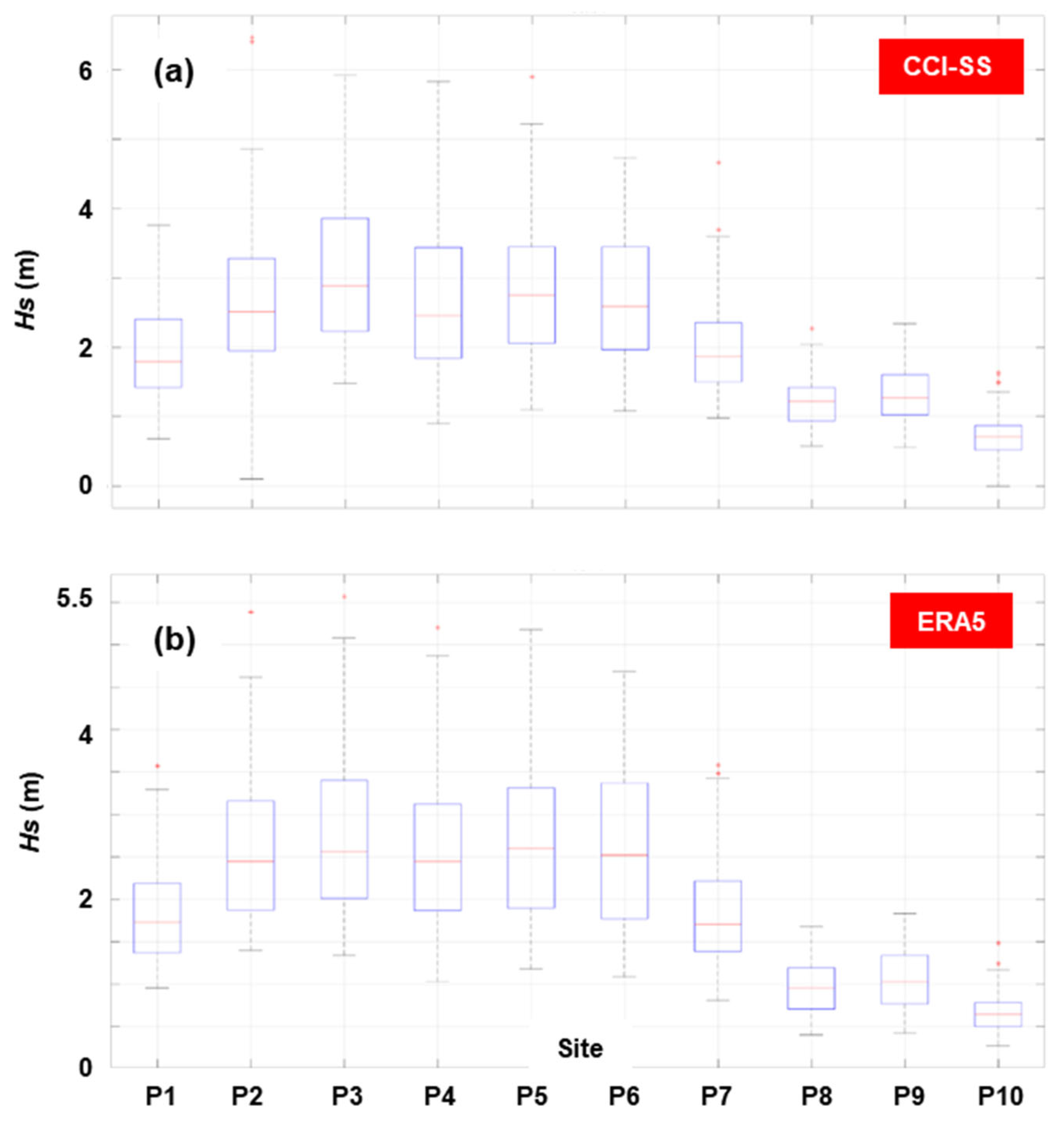
A direct comparison between the Hs parameters from the satellite and ERA5 datasets is shown in Figure 3. It can be seen that there is good agreement in terms of the spatial distribution, with site P3 (Ireland) showing higher values compared to site P10 (Bulgaria). In general, the values of the satellite measurements are higher, close to 2.88 m (P3) in terms of the 50th percentile, compared to ERA5, where similar values do not exceed 2.59 m (P5).

Figure 3. The Hs parameters (monthly values) represented by boxplots. (a) Satellite data; (b) ERA5 data. Results processed for the time interval 2002–2018 (17 years).

The values allow us to classify the reference sites into three groups: (a) P2–P6 (high wave conditions); (b) P1, P7 (average wave conditions); (c) P8–P10 (low wave conditions). This can be used as a quality indicator of the CCI-SS as a reliable source of data for ocean environments and enclosed sea basins.

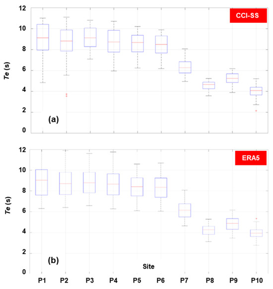
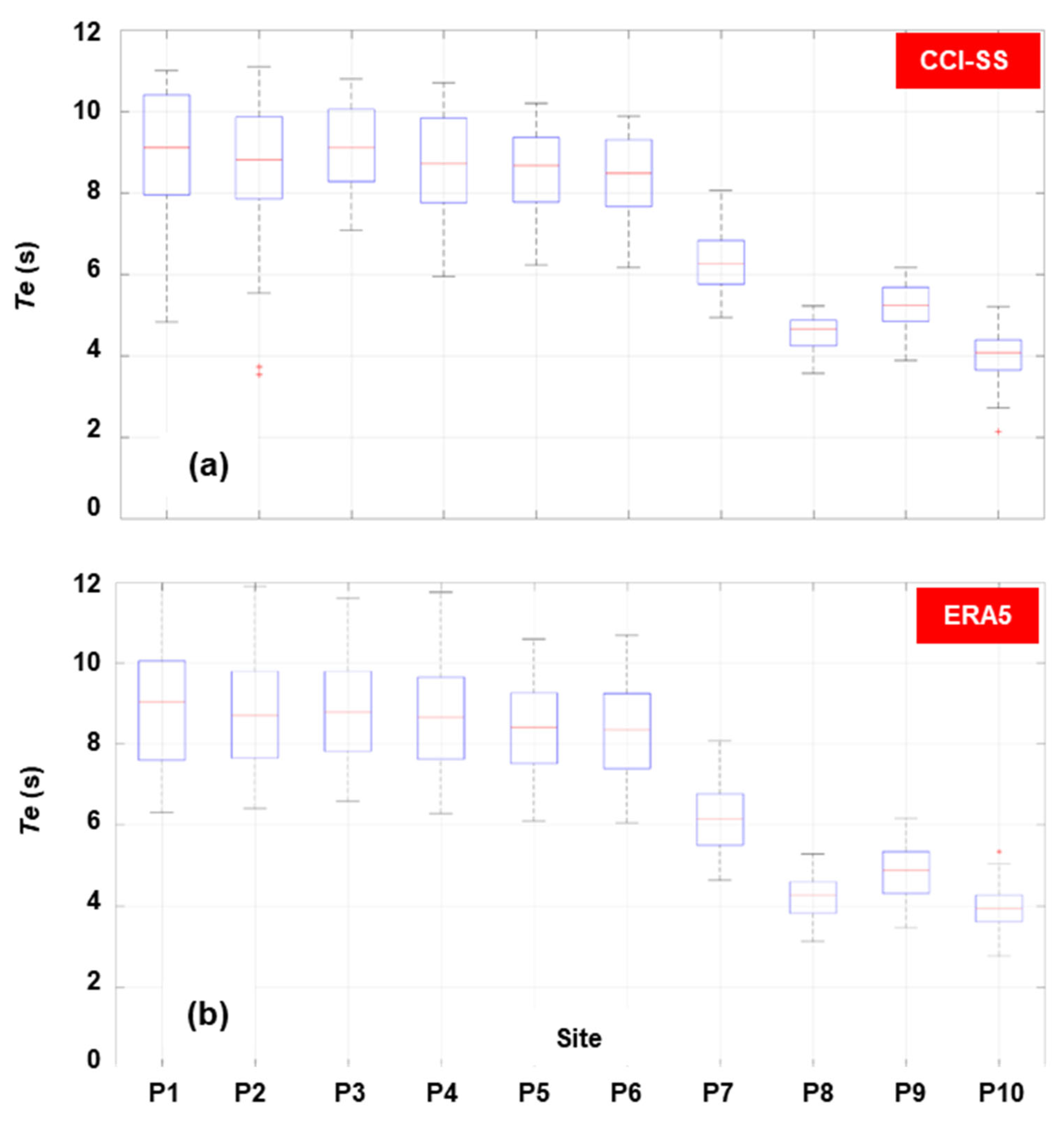
Figure 4 presents a similar analysis of the Te parameter. Regarding the spatial distribution of the two datasets, there is good agreement. The 50th percentile values are in the range of 4.08 to 9.11 s (satellite) compared to 3.92 to 9.04 s (ERA5), with higher values expected from the sites facing the ocean coastlines. Regarding the extreme values, the satellite data clearly show that site P1 is more significant (11 s), but sites P1–P4 in the ERA5 dataset can be regarded as being on the same level (11.6–12.01 s). From the enclosed seas, site P10 presents a minimum of 2.15 s (satellite) and 2.76 s (ERA5), being exceeded by the sites from the Mediterranean Sea that encounter minimums of 3.11 s (ERA5) and 3.58 s (satellite). In the analysis of the extreme values, however, it must be taken into account that the wave parameters are averaged values and not instantaneous values.

Figure 4. Te parameter boxplot representation (monthly values). (a) Satellite data; (b) ERA5 data. Results processed for the time interval 2002–2018 (17 years).

By considering the statistical values from Table 3 (50th and 95th percentile), a comprehensive picture of the Hs and Te analysis is completed. A direct comparison of the Hs values (50th percentile) shows that the satellite data indicate significantly higher values than ERA5, with site P4 showing good agreement.

Table 3. Statistical analysis of the Hs and Te parameters based on the CCI-SS and ERA5 data (monthly values). Results covering the time interval 2002–2018 (17 years).

Wave Parameter	Dataset	Percentile	Site
			P1	P2	P3	P4	P5	P6	P7	P8	P9	P10
Hs (m)	CCI-SS	50th	1.79	2.51	2.88	2.46	2.75	2.59	1.87	1.22	1.27	0.71
		95th	3.03	4.45	5.03	4.92	4.38	4.38	3.12	1.83	2.06	1.28
	ERA5	50th	1.73	2.45	2.56	2.45	2.6	2.52	1.71	0.95	1.03	0.65
		95th	2.78	3.95	4.59	4.09	4.07	4.28	2.84	1.47	1.68	1.04
Te (s)	CCI-SS	50th	9.12	8.82	9.12	8.71	8.67	8.48	6.26	4.66	5.25	4.08
		95th	10.9	10.9	10.7	10.6	9.98	9.8	7.51	5.16	6.06	4.97
	ERA5	50th	9.04	8.70	8.78	8.66	8.40	8.34	6.14	4.26	4.88	3.93
		95th	11.2	10.8	10.60	10.50	10.0	9.94	7.34	5.07	5.81	4.69

The 95th percentile shows the same pattern, with significantly smaller variations anticipated for site P6 (0.1 m). When it comes to the wave period, the satellite measurements (50th percentile) show much higher values than ERA5. However, in the case of the 95th percentile, the ERA5 values present more important wave periods only in the vicinity of site P1.

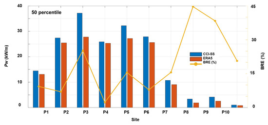
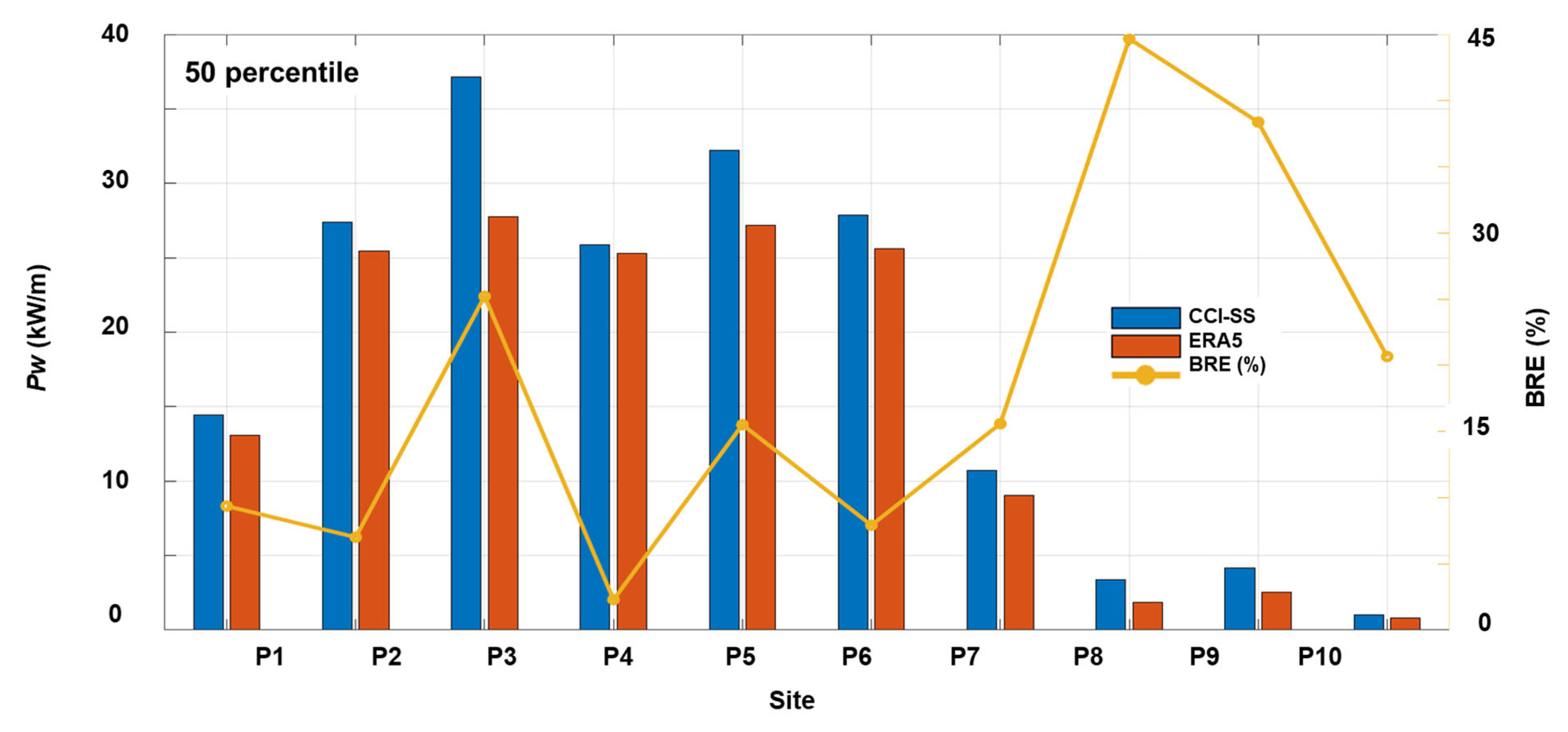
One way to evaluate the wave energy potential from a renewable perspective is the use of wave power. This is done in Figure 5, considering the 50th percentile distribution of the satellite (CCI-SS) and ERA5 datasets. As can be seen, the satellite-related values are higher than the ones from ERA5, regardless of the site taken into account. Higher values are observed in the vicinity of sites P2–P6, where the satellite values vary from 27.38 to 37.14 kW/m, while ERA5 spans the interval 25.3–27.8 kW/m. Smaller values are expected near site P10, where a minimum of 0.76 kW/m is related to the ERA5 data.

Figure 5. The satellite and ERA5 data (monthly values) distribution of the wave power reflected in terms of 50th percentile—in kW/m (left y-axis) and balance relative error—in % (right y-axis). Results processed for the time interval 2002–2018 (17 years).

The differences between the two datasets are indicated in terms of the balanced relative error (or BRE), which is defined as [48,49]

$$BRE=\left({\displaystyle \frac{X_{satellite}-X_{ERA5}}{X_{satellite}}}\right)\cdot 100$$

(8)

where Xsatellite is the CCI-SS measurements, and X_ERA5 is the ERA5 data. The sites from the enclosed seas, although with much lower wave energy, are characterized by higher differences in BRE (right y-axis) that can reach up to 44.67% in the case of site P8 (Zone C, France). Better agreement between the two datasets is noticed in the vicinity of sites P1, P2, P4, and P6, where the BRE indicator varies between 2.3% and 7.9%.

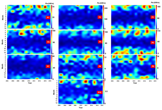
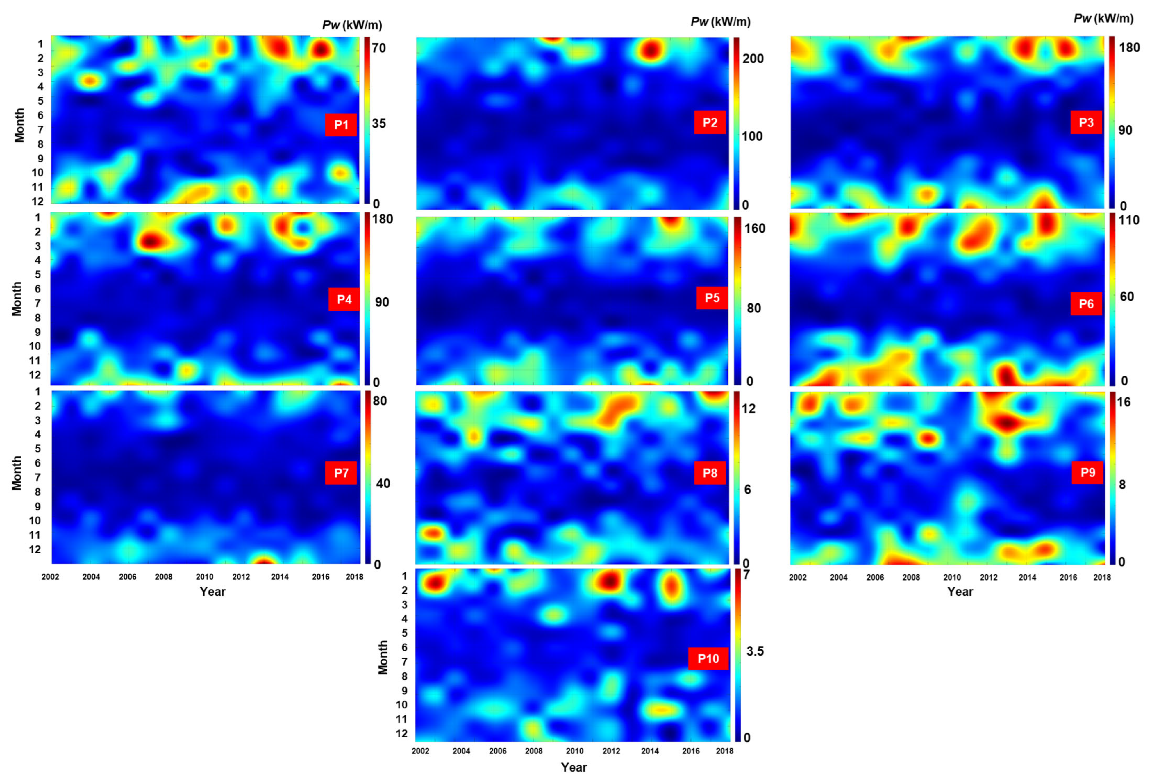
Figure 6 shows the monthly/annual distribution of the wave power, considering only the satellite measurements. As expected, they are closely linked to the location of each place that is identified, with monthly hotspots occurring during the winter months. For example, in the case of site P3, the general distribution is affected by the events occurring during the January–March interval, when the values can reach a maximum of 186.5 kW/m. Similar peak values may occur for the P4 and P5 sites, while a maximum of 110 kW/m is expected close to site P6 (Nordvest C, Norway). The sites from the Mediterranean Sea can reach a maximum of 16 kW/m, but per total, during the summer time, a particular sea state does not exceed 10 kW/m.

Figure 6. Wave power (50th percentile) monthly fluctuation of the satellite measurements. Results provided for all the reference sites, considering the total time interval (2002–2018).

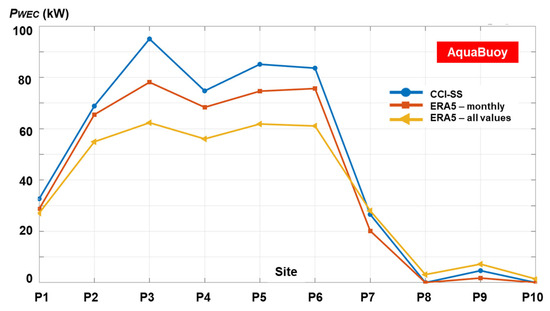
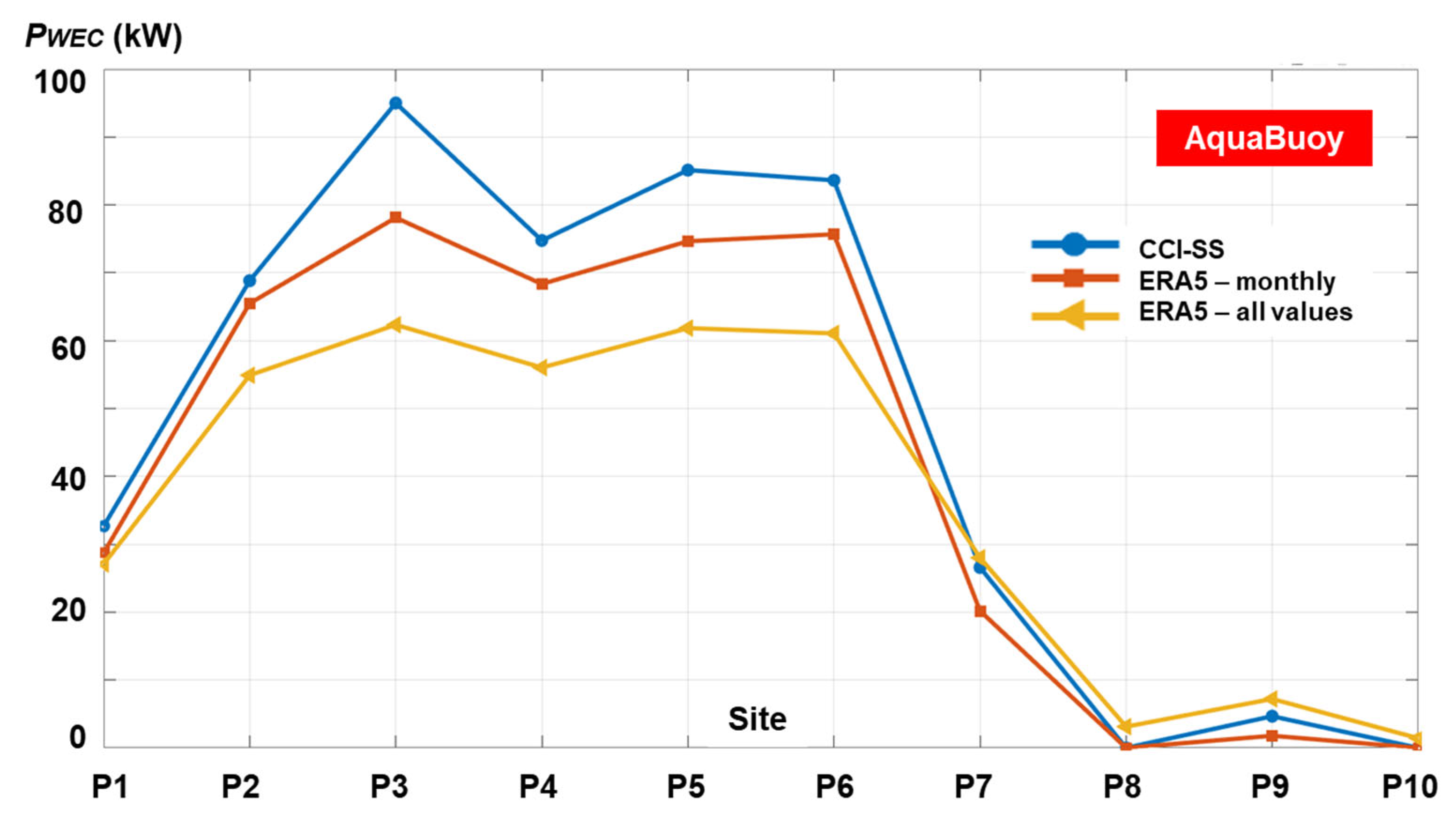
Establishing the accuracy of the satellite measurements (CCI-SS data, monthly values) in predicting a WEC generator’s long-term performance is another goal of the current work. Taking into account the AquaBuoy system and the ERA5 data, a first comparison is presented in Figure 7. In order to provide a complete picture, all the available ERA5 data were taken into account, namely (a) ERA5 monthly values and (b) all ERA5 values (eight values per day, 00-03-06-09-12-15-18-21 UTC). The expected power output is computed using the approach defined by Equation (6). It is evident that, for sites P1–P6, the wave power computed using the satellite measurements exceeds the values derived from the ERA5 datasets, reaching a maximum of 95 kW. For the remaining sites, the wave power estimated from the ERA5 (all values) datasets appears to be higher than that obtained from the other datasets.

Figure 7. AquaBuoy expected power output, considering (a) satellite data, (b) ERA5 data—monthly values; (c) ERA5 data—eight values per day (denoted as all values). The results are provided for all the reference sites and cover the total time interval (2002–2018).

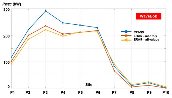
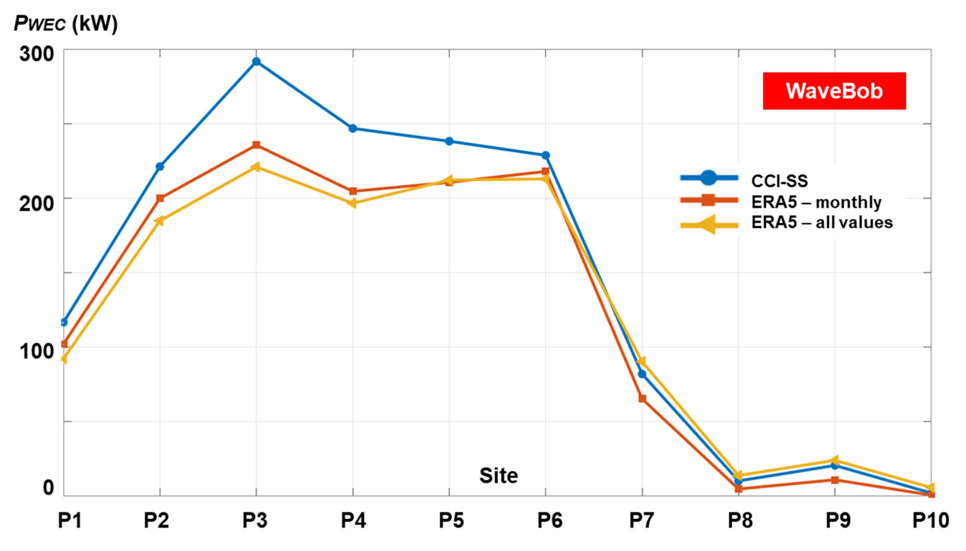
Another analysis is performed in Figure 8 for the WaveBob wave generator, and it can be seen that the overall distributions are comparable to the ones reported for the AquaBuoy system. The maximum values are substantially greater, but we must also consider the WaveBob’s rated power (1000 kW). For sites P1–P6, the estimated power output goes from 92.25 to 291.7 kW according to the site and database taken into account, and decreases to 0.7 kW in the case of site P10 (Black Sea). For sites P7–P10, the satellite and ERA5 (all values) present a similar evolution.

Figure 8. WaveBob expected power output, considering (a) satellite data, (b) ERA5 data—monthly values; (c) ERA5 data—eight values per day (denoted with all values). Results provided for all the reference sites, covering the total time interval (2002–2018).

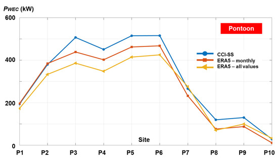
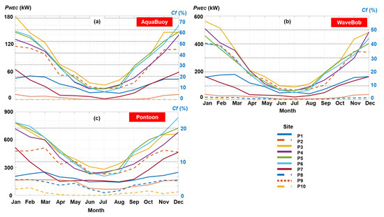
The Pontoon wave generator is the largest WEC considered for this study (rated power = 3619 kW), and its power production is shown in Figure 9.

Figure 9. Pontoon expected power output, considering (a) satellite data, (b) ERA5 data—monthly values; (c) ERA5 data—eight values per day (denoted with all values). Results provided for all the reference sites, covering the total time interval (2002–2018).

Compared to the prior WECs, the hierarchy of the databases is quite similar. The satellite data show greater values at sites P3, P4, P5, P6, P8, and P9, with a maximum of 515.3 kW. For the first time, ERA5 data (monthly values) show similar wave power values for sites P1 and P2, while the power output for site P7 is relatively similar to ERA5 (all values). The sites from the enclosed seas do not exceed 131 kW, with superior performance anticipated for the Mediterranean Sea.

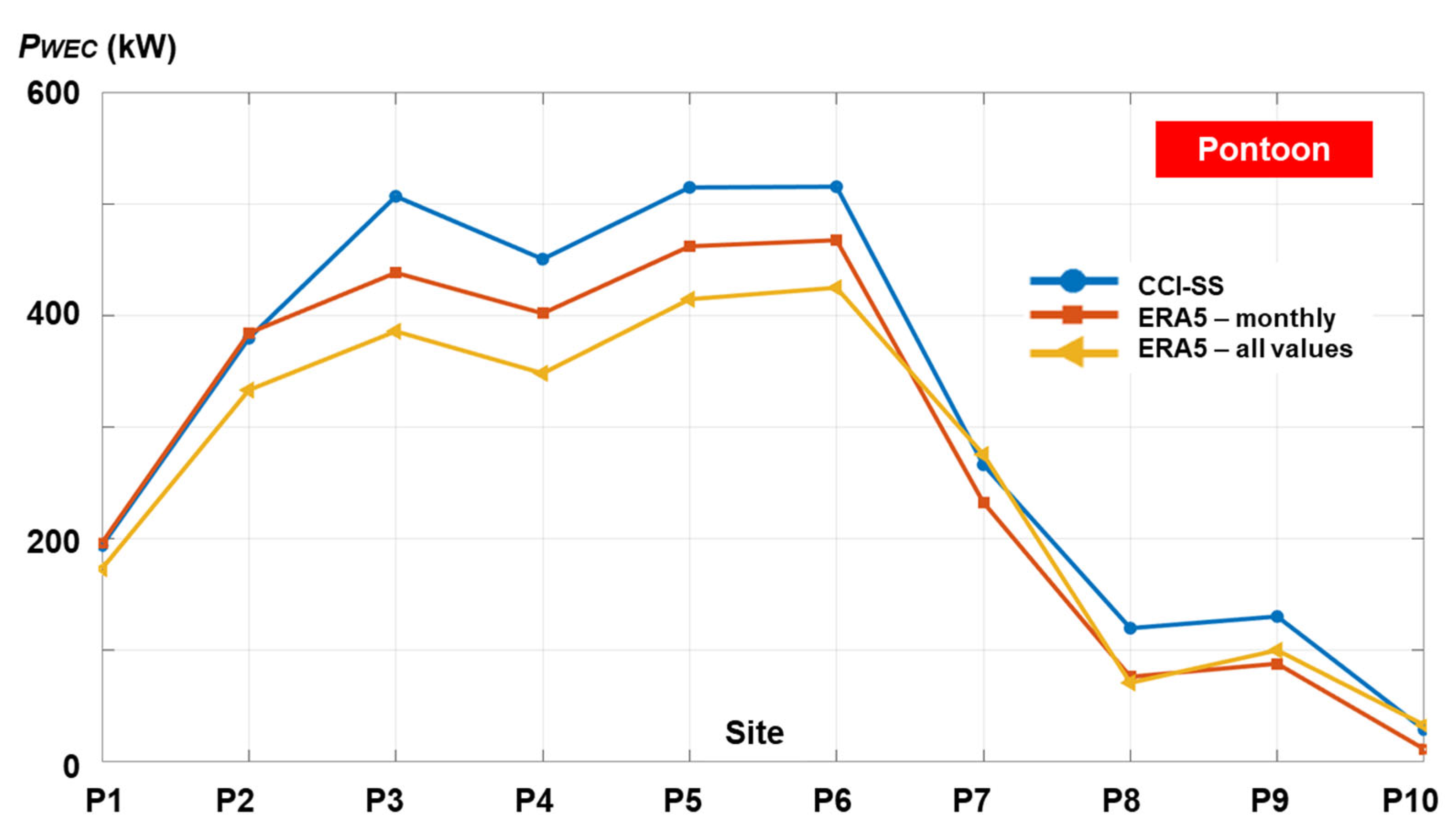
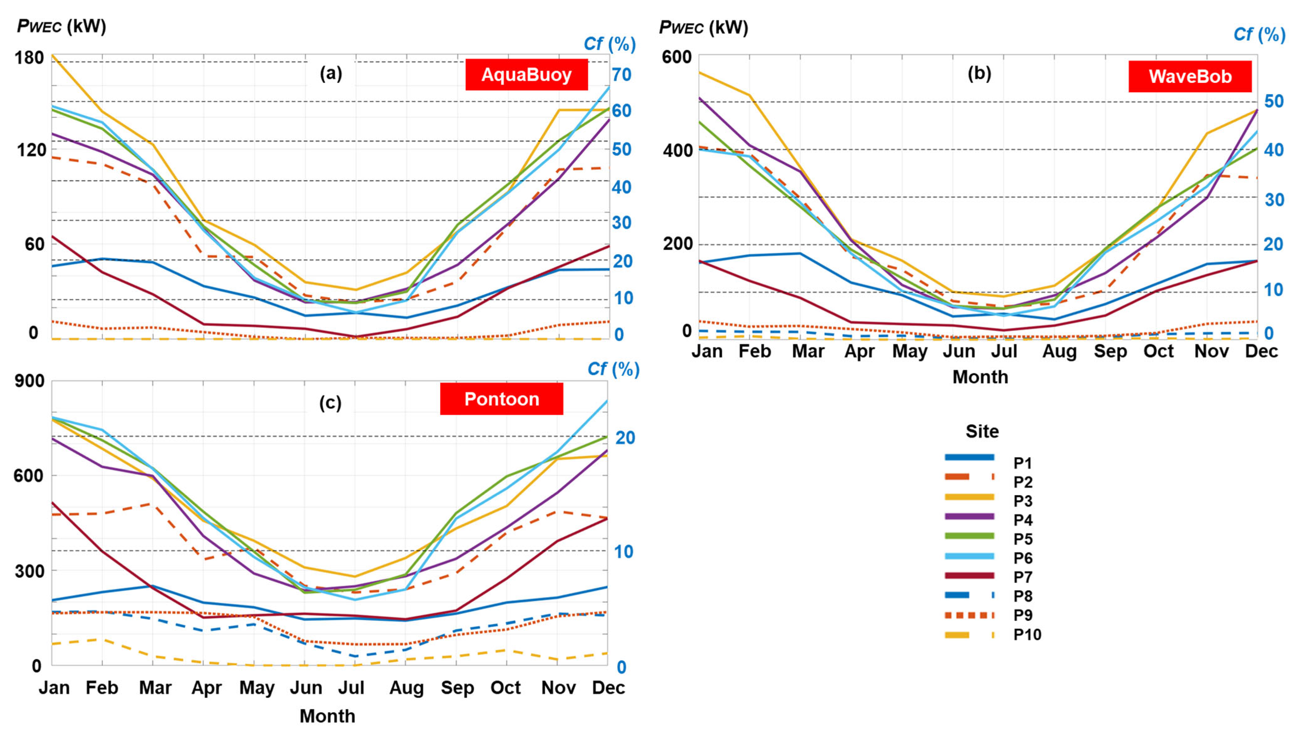
Figure 10 provides a complete picture of the considered WECs, taking into account their monthly performance. In addition to the power output, the capacity factor is also shown. The capacity factor is the ratio between the estimated power and the rated power output (maximum output), which is defined as [41]

$$Cf=\left({\displaystyle \frac{P_{WEC}}{P_R}}\right)\cdot 100$$

(9)

where P_WEC is the predicted power output (calculated), and P_R is the rated power of a WEC if it will operate at full capacity 100% of the time.

Figure 10. Monthly fluctuations of the WEC performances, taking into account the capacity factor (right y-axis, dashed lines) and predicted power output (left y-axis). (a) AquaBuoy (to be noticed that the line corresponding to P8 is the same as for P10 with zero values); (b) WaveBob; (c) Pontoon system. Results covering the time interval 2002–2018, based on satellite measurements.

It can be seen that the WECs’ performances are affected by the seasonal variations, with better results expected in winter time. For the sites located in the Mediterranean and the Black Sea, this fluctuation is less visible, expecting more constant values that do not exceed a capacity factor of 5%, independent of the WEC considered. The highest capacity factor is expected for the AquaBuoy system (up to 72%), followed by WaveBob with 56%, while the Pontoon wave generator is associated with a maximum of 23%. Regarding AquaBuoy, sites P2–P6 exhibit a power output in the range of 16.18 to 180 kW, whereas sites P8 and P10 have values that are nearly 0. When we move to the WaveBob device, the power production increases significantly. A maximum of 562.4 kW is seen in January, while sites P1 and P7 can reach high values of about 166 kW in January and December. The Pontoon generator appears to be a better choice for sites P3 and P4 (Ireland), where comparable results are anticipated.

4. Conclusions

Satellite measurements provide a reliable way to assess wave conditions on a global scale and can also be used for other applications, such as the development of marine renewable projects. This is the aim of the present work, where a total of 17 years of CCI-SS measurements (2002–2018) were taken into account in order to highlight the wave resources in the vicinity of some European sites located in different coastal environments (both ocean and enclosed seas). In order to determine if there is any bias in the geographical coverage of the CCI-SS dataset, which is produced by a multi-mission project, different sites were selected. A complete picture of a particular sea state can be made considering the parameters Hs and Te, but this is not possible with the satellite data, since they only give the Hs values. To solve this problem, it was possible to establish a correlation between the Hs and Te parameters associated with the ERA5 dataset, processed for the same time interval and reference sites.

The wave period represents an important element for the assessment of a particular WEC generator, taking into account that the power matrix associated with each WEC requires this parameter explicitly. In general, a multi-mission project that involves various altimeters will provide the satellite measurements in terms of average values that cover a particular temporal resolution (for example: day or month). By looking at the power matrix of a particular WEC, we can notice that the best performances are associated with the average sea states, while the extreme values (lower or higher) have a lower contribution to the overall electricity output of a wave generator. The sites selected are associated with some operational or perspective marine renewable sites that fall into the deep-water category. Site P10 (Black Sea) is not located in a deep-water area; however, we considered the same approach in order to see how well the satellite measurements are performing for this particular environment.

The CCI-SS and ERA5 data may now be directly compared in terms of Hs, Te, and wave power distribution. In terms of Hs geographical distribution, the results show very good agreement, with site P3 (Ireland) being more significant than site P10 (Black Sea), which is associated with the lowest values. As anticipated, both datasets classify the reference locations into two groups (open ocean and enclosed seas) based on the Te values. In general, the satellite observations show significantly higher values than those associated with ERA5, regardless of the parameter under consideration. The energy potential of a certain site is often evaluated using the wave power (or Pw). In this case, sites P8–P10 show significantly greater disparities (satellite and ERA5) that can reach 44.7% in favor of the satellite data. However, we must consider that these sites are characterized by substantially lower wave resources, with an average of less than 5 kW/m.

Estimating the performance of some WEC generators was another goal of the current work. The chosen WECs are intended to function in offshore environments and are categorized as point absorbers. Usually, the performance of a particular WEC is estimated by taking into account the wave datasets that are defined by higher temporal resolutions (ex: hourly scale). In the current work, we used monthly-averaged satellite measurements, which is regarded as a limitation of the proposed approach, because extreme climate conditions are not accounted for. By using data with higher temporal resolution, it is possible to take into account the occurrences of storm events or low-energy sea states. Nevertheless, similar to a wind turbine that is defined by cut-in and cut-out values, WEC generators are also defined to operate under some specific conditions. For example, if we look at the power matrix of the AquaBuoy system, we can notice that this will start to produce electricity from a sea state combination of Hs = 1 m and Tp = 5 s and will shut down if the significant wave height exceeds 5.5 m. It is expected that wave generators will be tuned for a particular sea state in order to obtain higher performances that, in the case of the AquaBuoy system, will be related to the Tp interval of 8–12 s and the Hs range of 4–4.5 m. A significant number of existing studies are dedicated to the long-term assessment of WEC performance using various datasets, and this aspect was investigated in the present work using satellite measurements.

As an element of novelty of the present work, it has to be highlighted that, as far as the authors are aware, this is the first publication that considers the potential of utilizing satellite measurements to predict the performance of a WEC system. The results show that the satellite measurements tend to overstate the power output of smaller and medium-sized WECs (rated power ≤ 300 kW), particularly those that face the ocean environment. The projected results for some sites are comparable to those linked to the ERA5 dataset as we move toward larger-capacity WECs (such as the Pontoon system). The power output for the Mediterranean Sea is slightly higher than that of ERA5, but this feature is only highlighted for this WEC.

Based on these findings, it can be concluded that the CCI-SS dataset presents good agreement in terms of the long-term prediction of wave resources and WEC performance using the current approach. Further studies should include calculation of the wave period directly from the Hs values supplied by the satellite observations. Finding appropriate end users and practical applications where satellite measurements can make a significant improvement will be another relevant topic for the future.

References

- Liang, G.; Li, S.; Bao, K.; Wang, G.; Teng, F.; Zhang, F.; Wang, Y.; Guan, S.; Wei, Z. Development of GNSS Buoy for Sea Surface Elevation Observation of Offshore Wind Farm. Remote Sens. 2023, 15, 5323. [Google Scholar] [CrossRef] [Scilit]
- Guillory, A. ERA5. Available online: https://www.ecmwf.int/en/forecasts/datasets/reanalysis-datasets/era5 (accessed on 31 May 2019).
- Hersbach, H.; Bell, B.; Berrisford, P.; Hirahara, S.; Horányi, A.; Muñoz-Sabater, J.; Nicolas, J.; Peubey, C.; Radu, R.; Schepers, D.; et al. The ERA5 Global Reanalysis. Q. J. R. Meteorol. Soc. 2020, 146, 1999–2049. [Google Scholar] [CrossRef] [Scilit]
- Celebrating 65 Years of the World’s First Weather Satellite. Available online: https://www.nesdis.noaa.gov/news/celebrating-65-years-of-the-worlds-first-weather-satellite (accessed on 10 May 2026).
- de Waard, J.; Mohr, T.; Diekmann, F.J.; Menzel, W.; Schmetz, J. Meteosat First Generation: Laying the Foundations of the European Geostationary Meteorological Satellite System. J. Eur. Meteorol. Soc. 2025, 3, 100025. [Google Scholar] [CrossRef] [Scilit]
- Liefhebber, F.; Lammens, S.; Brussee, P.W.G.; Bos, A.; John, V.O.; Rüthrich, F.; Onderwaater, J.; Grant, M.G.; Schulz, J. Automatic Quality Control of the Meteosat First Generation Measurements. Atmos. Meas. Tech. 2020, 13, 1167–1179. [Google Scholar] [CrossRef] [Scilit]
- Giri, R.K.; Prakash, S.; Yadav, R.; Kaushik, N.; Shukla, M.V.; Thapliyal, P.K.; Saikrishnan, K.C. A Review of the Global Operational Geostationary Meteorological Satellites. Remote Sens. Appl. Soc. Environ. 2025, 37, 101403. [Google Scholar] [CrossRef] [Scilit]
- Gkeka-Serpetsidaki, P.; Dimitriou, I.C.; Poursanidis, D.; Xirouchakis, S.; Skiniti, G.; Tournaki, S.; Tsoutsos, T. Development of Offshore Wind Farms from an Environmental Perspective. Renew. Energy 2026, 266, 125649. [Google Scholar] [CrossRef] [Scilit]
- Medina-Lopez, E.; McMillan, D.; Lazic, J.; Hart, E.; Zen, S.; Angeloudis, A.; Bannon, E.; Browell, J.; Dorling, S.; Dorrell, R.M.; et al. Satellite Data for the Offshore Renewable Energy Sector: Synergies and Innovation Opportunities. Remote Sens. Environ. 2021, 264, 112588. [Google Scholar] [CrossRef] [Scilit]
- Rusu, L.; Rusu, E. Evaluation of the Worldwide Wave Energy Distribution Based on ERA5 Data and Altimeter Measurements. Energies 2021, 14, 394. [Google Scholar] [CrossRef] [Scilit]
- Anık, E.M.; Amarouche, K.; Kankal, M.; Akpınar, A. Machine Learning-Based Residual Bias Correction of SWAN Significant Wave Height Using Satellite Altimeter Observations as Ground Truth in the Black Sea. Ocean Eng. 2026, 359, 125991. [Google Scholar] [CrossRef] [Scilit]
- Seemanth, M.; Remya, P.G.; Bhowmick, S.A.; Sharma, R.; Balakrishnan Nair, T.M.; Kumar, R.; Chakraborty, A. Implementation of Altimeter Data Assimilation on a Regional Wave Forecasting System and Its Impact on Wave and Swell Surge Forecast in the Indian Ocean. Ocean Eng. 2021, 237, 109585. [Google Scholar] [CrossRef] [Scilit]
- Li, S.; Guan, S.; Hou, Y.; Liu, Y.; Bi, F. Evaluation and Adjustment of Altimeter Measurement and Numerical Hindcast in Wave Height Trend Estimation in China’s Coastal Seas. Int. J. Appl. Earth Obs. Geoinf. 2018, 67, 161–172. [Google Scholar] [CrossRef] [Scilit]
- Liu, J.; Wu, M.; Wang, J. Impact of Assimilating CFOSAT SWIM Omnidirectional Spectra on Tropical Cyclone Wind–Wave Modeling. Ocean Model. 2026, 202, 102743. [Google Scholar] [CrossRef] [Scilit]
- Liu, L.; Wu, M.; Chen, G.; Tang, Y.; Song, X.; Zou, M.; Xu, Y.; Zhang, X.; Wang, S.; Lv, J.; et al. Satellite Observations and Deep Learning Unveil the Rapid Expansion of Offshore Wind Turbines in China. Resour. Conserv. Recycl. 2026, 227, 108706. [Google Scholar] [CrossRef] [Scilit]
- He, T.; Hu, Y.; Li, F.; Chen, Y.; Zhang, M.; Zheng, Q.; Jin, Y.; Ren, H. Mapping Land- and Offshore-Based Wind Turbines in China in 2023 with Sentinel-2 Satellite Data. Renew. Sustain. Energy Rev. 2025, 214, 115566. [Google Scholar] [CrossRef] [Scilit]
- Hasager, C.; Vincent, P.; Badger, J.; Badger, M.; Di Bella, A.; Peña, A.; Husson, R.; Volker, P. Using Satellite SAR to Characterize the Wind Flow around Offshore Wind Farms. Energies 2015, 8, 5413–5439. [Google Scholar] [CrossRef] [Scilit]
- Hasager, C.B. Offshore Winds Mapped from Satellite Remote Sensing. WIREs Energy Environ. 2014, 3, 594–603. [Google Scholar] [CrossRef] [Scilit]
- Pleskachevsky, A.; Tings, B.; Wiehle, S.; Imber, J.; Jacobsen, S. Multiparametric Sea State Fields from Synthetic Aperture Radar for Maritime Situational Awareness. Remote Sens. Environ. 2022, 280, 113200. [Google Scholar] [CrossRef] [Scilit]
- Ribal, A.; Young, I. 33 Years of Globally Calibrated Wave Height and Wind Speed Data Based on Altimeter Observations. Sci. Data 2019, 6, 77. [Google Scholar] [CrossRef] [Scilit] [PubMed]
- Jiang, H. Evaluation of Altimeter Undersampling in Estimating Global Wind and Wave Climate Using Virtual Observation. Remote Sens. Environ. 2020, 245, 111840. [Google Scholar] [CrossRef] [Scilit]
- Ponce De León, S.; Bettencourt, J.H.; Ringwood, J.V.; Benveniste, J. Assessment of Combined Wind and Wave Energy in European Coastal Waters Using Satellite Altimetry. Appl. Ocean Res. 2024, 152, 104184. [Google Scholar] [CrossRef] [Scilit]
- Ozbahceci, B.O. Extreme Value Statistics of Wind Speed and Wave Height of the Marmara Sea Based on Combined Radar Altimeter Data. Adv. Space Res. 2020, 66, 2302–2318. [Google Scholar] [CrossRef] [Scilit]
- Elshinnawy, A.I.; Antolínez, J.A.Á. A Changing Wave Climate in the Mediterranean Sea during 58-Years Using UERRA-MESCAN-SURFEX High-Resolution Wind Fields. Ocean Eng. 2023, 271, 113689. [Google Scholar] [CrossRef] [Scilit]
- Wiese, A.; Staneva, J.; Schulz-Stellenfleth, J.; Behrens, A.; Fenoglio-Marc, L.; Bidlot, J.-R. Synergy of Wind Wave Model Simulations and Satellite Observations during Extreme Events. Ocean Sci. 2018, 14, 1503–1521. [Google Scholar] [CrossRef] [Scilit]
- Gallagher, S.; Tiron, R.; Whelan, E.; Gleeson, E.; Dias, F.; McGrath, R. The Nearshore Wind and Wave Energy Potential of Ireland: A High Resolution Assessment of Availability and Accessibility. Renew. Energy 2016, 88, 494–516. [Google Scholar] [CrossRef] [Scilit]
- Rusu, L.; Onea, F.; Rusu, E. The Expected Impact of Marine Energy Farms Operating in Island Environments with Mild Wave Energy Resources—A Case Study in the Mediterranean Sea. Inventions 2021, 6, 33. [Google Scholar] [CrossRef] [Scilit]
- Passaro, M.; Dodet, G.; Ardhuin, F.; Cipollini, P. WHALES: An Enhanced Retracker for Satellite Radar Altimeter Delay-Only Waveforms in Sea State Applications. Remote Sens. Environ. 2026, 342, 115482. [Google Scholar] [CrossRef] [Scilit]
- Ardhuin, F.; Postec, T.; Accensi, M.; Piolle, J.-F.; Dodet, G.; Passaro, M.; De Carlo, M.; Husson, R.; Guitton, G.; Collard, F. Sizing the Largest Ocean Waves Using the SWOT Mission. Proc. Natl. Acad. Sci. USA 2025, 122, e2513381122. [Google Scholar] [CrossRef] [Scilit] [PubMed]
- Gommenginger, C.P.; Srokosz, M.A.; Challenor, P.G.; Cotton, P.D. Measuring Ocean Wave Period with Satellite Altimeters: A Simple Empirical Model. Geophys. Res. Lett. 2003, 30, 2003GL017743. [Google Scholar] [CrossRef] [Scilit]
- Wang, X.; Ichikawa, K. Effect of High-Frequency Sea Waves on Wave Period Retrieval from Radar Altimeter and Buoy Data. Remote Sens. 2016, 8, 764. [Google Scholar] [CrossRef] [Scilit]
- Raileanu, A.; Onea, F.; Rusu, E. An Overview of the Expected Shoreline Impact of the Marine Energy Farms Operating in Different Coastal Environments. JMSE 2020, 8, 228. [Google Scholar] [CrossRef] [Scilit]
- Veigas, M.; Carballo, R.; Iglesias, G. Wave and Offshore Wind Energy on an Island. Energy Sustain. Dev. 2014, 22, 57–65. [Google Scholar] [CrossRef] [Scilit]
- Yüksek, O.; Amarouche, K.; Akpınar, A. Wind, Wave, and Hybrid Energy Systems’ Assessment in the NE-Mediterranean Sea. Ocean Eng. 2026, 358, 125652. [Google Scholar] [CrossRef] [Scilit]
- Black Sea fLoating Offshore Wind|BLOW|Project|Fact Sheet|HORIZON. Available online: https://cordis.europa.eu/project/id/101084323 (accessed on 16 May 2026).
- Birol, F.; Bignalet-Cazalet, F.; Cancet, M.; Daguze, J.-A.; Fkaier, W.; Fouchet, E.; Léger, F.; Maraldi, C.; Niño, F.; Pujol, M.-I.; et al. Understanding Uncertainties in the Satellite Altimeter Measurement of Coastal Sea Level: Insights from a Round-Robin Analysis. Ocean Sci. 2025, 21, 133–150. [Google Scholar] [CrossRef] [Scilit]
- Bonnefond, P.; Exertier, P.; Laurain, O.; Thibaut, P.; Mercier, F. GPS-Based Sea Level Measurements to Help the Characterization of Land Contamination in Coastal Areas. Adv. Space Res. 2013, 51, 1383–1399. [Google Scholar] [CrossRef] [Scilit]
- Dodet, G.; Mureau, G.; Accensi, M.; Piollé, J.-F. Impact of Altimeter-Buoy Data-Pairing Methods on the Validation of Sentinel-3A Coastal Significant Wave Heights. Remote Sens. Environ. 2025, 316, 114483. [Google Scholar] [CrossRef] [Scilit]
- Passaro, M.; Hemer, M.A.; Quartly, G.D.; Schwatke, C.; Dettmering, D.; Seitz, F. Global Coastal Attenuation of Wind-Waves Observed with Radar Altimetry. Nat. Commun. 2021, 12, 3812. [Google Scholar] [CrossRef] [Scilit] [PubMed]
- Dodet, G.; Piolle, J.-F.; Quilfen, Y.; Abdalla, S.; Accensi, M.; Ardhuin, F.; Ash, E.; Bidlot, J.-R.; Gommenginger, C.; Marechal, G.; et al. The Sea State CCI Dataset v1: Towards a Sea State Climate Data Record Based on Satellite Observations. Earth Syst. Sci. Data 2020, 12, 1929–1951. [Google Scholar] [CrossRef] [Scilit]
- Rusu, L.; Onea, F. The Performance of Some State-of-the-Art Wave Energy Converters in Locations with the Worldwide Highest Wave Power. Renew. Sustain. Energy Rev. 2017, 75, 1348–1362. [Google Scholar] [CrossRef] [Scilit]
- USACE Publications—Engineer Manuals. Available online: https://www.publications.usace.army.mil/USACE-Publications/Engineer-Manuals/ (accessed on 21 June 2026).
- Polyfit—Polynomial Curve Fitting—MATLAB. Available online: https://www.mathworks.com/help/matlab/ref/polyfit.html (accessed on 21 June 2026).
- Rusu, E.; Onea, F. Estimation of the Wave Energy Conversion Efficiency in the Atlantic Ocean Close to the European Islands. Renew. Energy 2016, 85, 687–703. [Google Scholar] [CrossRef] [Scilit]
- Chen, C.Y.J. Determination of the Right Wave by Empirical Statistics: The Wave Energy Resource Assessment and the Investigation of Existing Marine and Coastal Potential Compatibility. J. Ocean Eng. Sci. 2016, 1, 284–288. [Google Scholar] [CrossRef] [Scilit]
- Majidi, A.G.; Ramos, V.; Rosa-Santos, P.; das Neves, L.; Taveira-Pinto, F. Power Production Assessment of Wave Energy Converters in Mainland Portugal. Renew. Energy 2025, 243, 122540. [Google Scholar] [CrossRef] [Scilit]
- Evaluate Curve Fit—MATLAB & Simulink. Available online: https://www.mathworks.com/help/curvefit/evaluate-a-curve-fit.html (accessed on 21 June 2026).
- Yildirir, V.; Rusu, E.; Onea, F. Wind Energy Assessments in the Northern Romanian Coastal Environment Based on 20 Years of Data Coming from Different Sources. Sustainability 2022, 14, 4249. [Google Scholar] [CrossRef] [Scilit]
- Silhavy, R.; Silhavy, P.; Prokopova, Z. Computational Statistics and Mathematical Modeling Methods in Intelligent Systems. In Advances in Intelligent Systems and Computing (AISC); Springer: Cham, Switzerland, 2019; Volume 1047, ISBN 978-3-030-31361-6. [Google Scholar]
Disclaimer/Publisher’s Note: The statements, opinions and data contained in all publications are solely those of the individual author(s) and contributor(s) and not of MDPI and/or the editor(s). MDPI and/or the editor(s) disclaim responsibility for any injury to people or property resulting from any ideas, methods, instructions or products referred to in the content. |
© 2026 by the authors. Licensee MDPI, Basel, Switzerland. This article is an open access article distributed under the terms and conditions of the Creative Commons Attribution (CC BY) license.