Short-Term Motion Prediction of an FLNG System for Collision Risk Mitigation During Side-by-Side Offloading Operations

Abstract

Floating liquefied natural gas (FLNG) facilities integrate natural gas liquefaction, storage, and offloading into a single vessel. During ship-to-ship (STS) side-by-side offloading, an LNG carrier (LNGC) moors alongside the FLNG to transfer liquefied cargo through a loading-arm system. The hydrodynamic interactions between the two vessels, combined with environmental loads, can lead to excessive relative motions that pose a risk of collision or damage to the loading arms and fenders. Accurate short-term prediction of vessel motions would provide operators with advance warning of potentially dangerous conditions, allowing preventive actions to be taken. This study presents a data-driven approach to short-term motion prediction using experimental data obtained from comprehensive basin model tests of an FLNG system. The model tests covered 15 environmental conditions, including survival conditions (100-year return period) and operating conditions (1-year return period), under both single-vessel and side-by-side configurations. Three prediction methods were evaluated: an autoregressive linear model, a single-degree-of-freedom multi-layer perceptron, and a multi-head attention cross-coupling network (MAC-Net) that leverages temporal attention, cross-DOF graph message passing, and multi-task learning with uncertainty-weighted loss. The results show that surge, sway, and yaw can be predicted with high skill scores at model-scale horizons of up to 4 s (32 s full-scale equivalent), while heave and pitch exhibit limited predictability beyond 2 s model scale. The MAC-Net model demonstrates particular advantages for roll prediction, achieving a skill score of 0.88 at a 4 s model-scale horizon compared to 0.76 for the conventional method, attributable to the physical coupling between roll and the horizontal-plane motions through the mooring system. These findings support a practical early warning concept in which horizontal-plane motions provide advance collision alerts and heave/pitch are treated as short-horizon monitoring quantities.

1. Introduction

As floating liquefied natural gas (FLNG) facilities increasingly operate in harsh, open-ocean environments, the safety of ship-to-ship (STS) side-by-side offloading operations has become a critical operational bottleneck. In the configuration considered here, an LNG carrier (LNGC) is berthed alongside a turret-moored FLNG and liquefied cargo is transferred through a loading-arm system while the hulls are separated by fenders and hawsers. While the FLNG’s internal turret single-point mooring (SPM) system allows the combined vessels to weathervane against prevailing winds, waves, and currents, the narrow side-by-side gap leaves little margin for error. This configuration differs from conventional terminal-to-ship STS transfer because the larger unit is a weathervaning offshore production/storage facility rather than a fixed berth or a freely drifting tanker pair.

This tight proximity introduces highly complex hydrodynamic interactions. The adjacent hulls significantly modify the local wave field, frequently trapping water and triggering severe gap resonance that amplifies wave elevations [1,2,3]. Consequently, excessive relative motions—particularly in surge, sway, and yaw—can rapidly overload mooring hawsers and fenders, raising the risk of hull collisions. The severity of these interactions is extremely sensitive to environmental conditions, ranging from multi-field coupled loads in standard operating windows [4] to extreme scenarios involving ice-covered waters. Previous studies have extensively modeled these dynamics, highlighting the critical influence of viscous damping [1], second-order drift forces [5,6], mooring system nonlinearities [7], and the specific vulnerability of the combined system to quartering seas [8].

To mitigate these collision risks, operators require actionable foresight: an early warning system capable of forecasting vessel motions tens of seconds in advance. In practice, such warnings would be tied to concrete actions such as suspending cargo transfer, checking hawser and fender loads, preparing loading-arm disconnection, or increasing the monitoring state when predicted relative lateral displacement approaches a site-specific allowable envelope [9,10]. Traditional spectral methods grounded in potential flow theory [11,12,13] excel at determining statistical motion distributions but fall short in generating the deterministic, time-domain trajectories needed for real-time avoidance. As a result, the focus has shifted toward data-driven approaches that learn directly from temporal motion sequences [14].

In recent years, deep learning architectures—particularly long short-term memory (LSTM) networks [15] and gated recurrent units (GRUs)—have established a strong baseline for maritime time-series forecasting [16]. To further extend prediction horizons and improve accuracy, researchers have actively augmented these recurrent structures. Recent innovations have integrated attention mechanisms and convolutional layers to better extract spatio-temporal features [17,18], employed temporal convolutional networks (TCNs) for alternative sequence modeling [19,20], and utilized wavelet transformations to assist in frequency-domain feature extraction and semi-stationary sea state identification [21,22]. Furthermore, the field has seen emerging applications of quaternion transformers [23], physics-informed architectures [24], and spectral wave radar data fusion [25].

Yet, a fundamental disconnect persists between algorithmic development and physical reality. The vast majority of these predictive models are trained purely on idealized numerical simulations, rarely confronting the noisy, coupled dynamics of physical side-by-side systems. Furthermore, the distinctive cross-coupling effects inherent to turret-moored, multi-body configurations are often overlooked in standard predictive frameworks. To bridge this gap, we present an integrated experimental and data-driven study focused specifically on FLNG side-by-side offloading. The main contributions of this paper are as follows:

• We present a comprehensive experimental dataset from basin model tests of an FLNG-LNGC system, covering 15 environmental conditions across both survival and operating scenarios. To the best of our knowledge, this serves as one of the most extensive publicly documented physical datasets for FLNG motion responses.
• We systematically evaluate three distinct prediction architectures—ranging from baseline autoregressive models to a novel multi-head attention cross-coupling network (MAC-Net)—quantitatively comparing their performance across all six degrees of freedom and multiple prediction horizons.
• We identify and quantify the cross-coupling effect in roll prediction. We demonstrate that incorporating multi-DOF inputs significantly enhances roll forecasting accuracy, a finding physically corroborated by the horizontal-to-roll coupling induced by the turret mooring system.
• We assess the implications of these predictions for collision risk during offloading, detailing the practical requirements for deploying such models in a real-time motion-based early warning system.

The remainder of this paper is organized as follows. Section 2 details the basin experimental setup and data acquisition. Section 3 outlines the formulation of the proposed prediction networks. Section 4 presents the comparative forecasting results and hydrodynamic discussion, followed by conclusions in Section 5.

2. Experimental Setup and Data

2.1. Model Test Overview

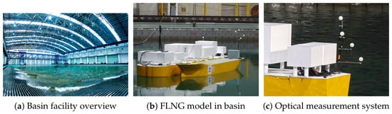
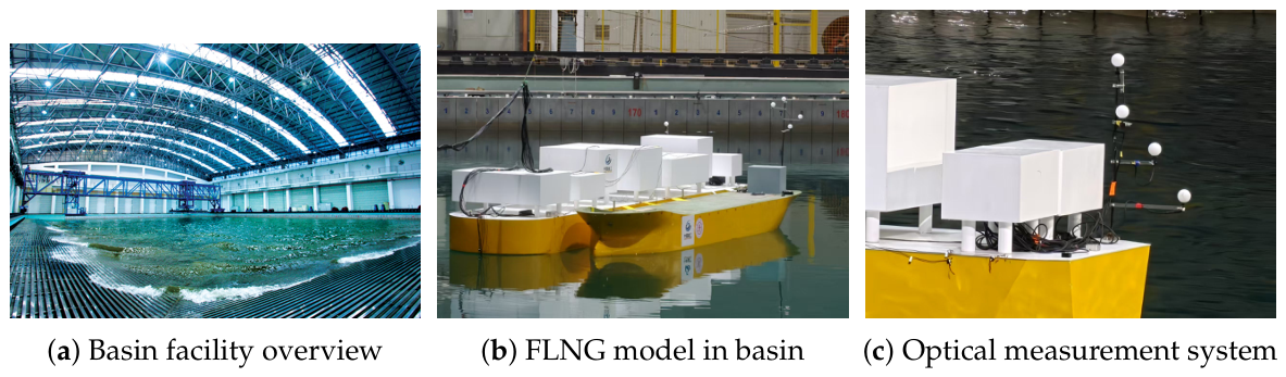
Figure 1 shows the basin facility and model setup used in the experiments. The model tests were conducted in the deep-water basin at Shanghai Jiao Tong University (SKLOE), located in Shanghai, China. The basin dimensions are 50 m in length, 40 m in width, and 10 m in depth, equipped with a multidirectional wave generator capable of generating both regular and irregular waves, a wind generation system, and a current generation system. The basin is fitted with a movable false bottom that allows the water depth to be adjusted from 0 to 10 m. A non-contact optical six-degree-of-freedom measurement system was used to record the motions of both vessels simultaneously, as shown in Figure 1c.

The scale ratio for the model tests was 1:64, following Froude number similarity. The corresponding time-scale factor is $\sqrt{64}=8$, so 1 s in model scale corresponds to 8 s at full scale. Model-scale motions were recorded in centimeters (cm) for translational degrees of freedom and degrees for rotational degrees of freedom. The sampling frequency was 50 Hz in the model scale. Each irregular wave test lasted at least 1800 s in model scale, yielding more than 90,000 data points per test condition. Unless explicitly stated otherwise, motion amplitudes and prediction horizons reported in the following sections are model-scale values; full-scale equivalent times can be obtained by multiplying by 8.

2.2. Vessel and Mooring System

The FLNG vessel has a length overall of 374.50 m, a beam of 68.00 m, and a depth of 38.75 m. Two loading conditions were tested: full load (draft 17.00 m, displacement 384,686 t) and ballast (draft 12.00 m, displacement 267,602 t). The vessel is moored by an internal turret single-point mooring system consisting of 3 groups of 4 lines, with a 120-degree angle between groups and a 5-degree spread within each group. The mooring lines are a combination of chain and polyester rope segments, with a pre-tension of 225 t and a mooring radius of 6000 m at the target water depth of 2100 m.

Due to the limited depth of the test basin, a truncated mooring design was adopted. The truncation preserved the horizontal restoring force characteristics of the full-depth system while reducing the mooring radius to 14.27 m in the model scale. The static stiffness curves of the truncated mooring system were verified against the target stiffness through horizontal pull-out tests in calm water, with the maximum deviation in the sway direction being less than 5%.

The LNGC has a length overall of 307 m, a beam of 54 m, and a depth of 28.8 m. In the side-by-side offloading tests, the FLNG was in the full load condition and the LNGC was in ballast (draft 7.75 m). The assumed operational configuration is an offshore STS offloading arrangement in which the LNGC is moored on the side of the terminal-like FLNG by hawsers, the hull gap is maintained by fenders, and the limiting motion envelope is governed primarily by allowable fender compression and loading-arm travel. The principal particulars of both vessels are summarized in

Table 1. Principal particulars of the FLNG and LNGC vessels.

Parameter	FLNG		LNGC
	Full Load	Ballast	Full Load	Ballast
Length overall (m)	374.50	374.50	307.00	307.00
Length between perpendiculars (m)	357.50	357.50	300.00	300.00
Beam (m)	68.00	68.00	54.00	54.00
Depth (m)	38.75	38.75	28.80	28.80
Draft (m)	17.00	12.00	9.50	7.75
Displacement (t)	384,686	267,602	118,278	95,384
LCG from midship (m)	171.89	171.96	163.00	163.50
VCG above keel (m)	23.09	25.67	12.50	12.11
Roll radius of gyration (m)	22.22	25.67	16.10	16.10
Pitch radius of gyration (m)	99.22	100.98	74.25	74.25
Yaw radius of gyration (m)	98.83	100.13	74.25	74.25
Natural period in heave (s)	12.5	11.6	10.06	9.71
Natural period in roll (s)	16.8	14.3	7.85	7.65
Natural period in pitch (s)	12.2	11.4	9.37	9.03

.

2.3. Environmental Conditions

Two categories of environmental conditions were tested: survival conditions corresponding to a 100-year return period and operating conditions corresponding to a 1-year return period. The survival conditions featured a significant wave height of 4.7 m and a spectral peak period of 14.2 s, with a wind speed of 14.9 m/s and a surface current speed of 1.45 m/s. The operating conditions had a significant wave height of 3.1 m, a peak period of 12.2 s, a wind speed of 10.7 m/s, and a current speed of 0.95 m/s. Irregular waves were generated following the JONSWAP spectrum with a peak enhancement factor of 3.3.

The environmental headings were defined relative to the mooring system. Three heading configurations were tested: in-line (wave, wind, and current all aligned with the mooring axis, 0 degrees), between-line (60 degrees from the mooring axis), and quartering (wave and wind at 30 degrees, current remaining at 0 degrees due to the fixed direction of the basin current generation system). Additionally, individual wave-only, wind-only, and current-only tests were performed to decompose the contribution of each environmental component.

Table 2. Environmental conditions for model tests.

Condition	${\mathit{H}}_{\mathit{s}}$ (m)	${\mathit{T}}_{\mathit{p}}$ (s)	Wind (m/s)	Current (m/s)	Wave Dir. (°)	Wind Dir. (°)
100-Year Return Period (Survival)
DL11 (Wave only)	4.7	14.2	-	-	0	-
DL12 (Wind only)	-	-	14.9	-	-	0
DL13 (Current only)	-	-	-	1.45	-	-
DL14 (In-Line)	4.7	14.2	14.9	1.45	0	0
DL15 (Between-Line)	4.7	14.2	14.9	1.45	60	60
DL16 (Quartering)	4.7	14.2	14.9	1.45	30	30
DL19 (Wave only, ballast)	4.7	14.2	-	-	0	-
DL20 (Wind only, ballast)	-	-	14.9	-	-	0
DL21 (Current only, ballast)	-	-	-	1.45	-	-
DL22 (In-Line, ballast)	4.7	14.2	14.9	1.45	0	0
DL23 (Between-Line, ballast)	4.7	14.2	14.9	1.45	60	60
DL24 (Quartering, ballast)	4.7	14.2	14.9	1.45	30	30
1-Year Return Period (Operating)
DL25 (In-Line)	3.1	12.2	10.7	0.95	0	0
DL26 (Between-Line)	3.1	12.2	10.7	0.95	60	60
DL27 (Quartering)	3.1	12.2	10.7	0.95	30	0

provides a complete summary of all 15 test conditions. A total of 12 conditions involved the FLNG vessel alone (DL11–DL24, covering both full load and ballast), and 3 conditions involved the side-by-side configuration with the LNGC (DL25–DL27).

2.4. Measured Data

The six-degree-of-freedom motions measured at the center of gravity of each vessel include surge, sway, heave, roll, pitch, and yaw, defined in the body-fixed coordinate system. Surge and sway are translations along and perpendicular to the vessel longitudinal axis, respectively; heave is the vertical translation; roll, pitch, and yaw are rotations about the longitudinal, transverse, and vertical axes, respectively.

For the side-by-side conditions (DL25–DL27), the motions of both the FLNG and the LNGC were recorded simultaneously. The relative motions between the two vessels, which are directly relevant to collision risk assessment, were computed as the difference between the corresponding FLNG and LNGC motion time-series.

3. Prediction Methodology

3.1. Problem Formulation

The motion prediction task is formulated as a time-series forecasting problem. Given the past L time steps of motion data $\mathbf{x}(t-L+1),\mathbf{x}(t-L+2),\dots ,\mathbf{x}\left(t\right)$, the goal is to predict the motion at a future time step $t+h$, where h is the prediction horizon. The motion vector $\mathbf{x}\left(t\right)={[x_1\left(t\right),x_2\left(t\right),\dots ,x_6\left(t\right)]}^{\top }$ contains all six degrees of freedom (surge, sway, heave, roll, pitch, yaw).

For a single degree of freedom $x_i$, the prediction mapping can be expressed as:

$${\widehat{x}}_i(t+h)={\mathcal{F}}_i\left({\mathbf{z}}_i\left(t\right)\right)$$

(1)

where ${\mathbf{z}}_i\left(t\right)={[x_i(t-L+1),x_i(t-L+2),\dots ,x_i\left(t\right)]}^{\top }\in {\mathbb{R}}^L$ is the input feature vector constructed from the past L observations, and ${\mathcal{F}}_i$ is the prediction function to be determined. For the multi-degree-of-freedom case, the input is extended to include cross-coupling information:

$$\mathbf{Z}\left(t\right)={[{\mathbf{x}}^{\top }(t-L+1),{\mathbf{x}}^{\top }(t-L+2),\dots ,{\mathbf{x}}^{\top }\left(t\right)]}^{\top }\in {\mathbb{R}}^{6L}$$

(2)

and the prediction becomes ${\widehat{x}}_i(t+h)={\mathcal{G}}_i\left(\mathbf{Z}\left(t\right)\right)$.

In the context of FLNG collision risk, the prediction horizon is determined by the response time required for operational actions. The horizons used in this study are specified in model-scale seconds because the input data are sampled in model time. Under the 1:64 Froude scaling, the tested horizons of 0.2, 1, 2, 4, and 10 s correspond to full-scale lead times of 1.6, 8, 16, 32, and 80 s, respectively. Thus, model-scale horizons of 1–2 s are suitable for short-horizon monitoring, whereas 4–10 s model scale horizons provide full-scale lead times relevant to human operator decisions and emergency procedures.

3.2. Data Preprocessing

The raw motion data were preprocessed before training. The time-series were downsampled from 50 Hz to 5 Hz by taking every 10th sample, reducing computational cost without losing useful information since the dominant wave energy in the 100-year return period spectrum is concentrated below 0.15 Hz (full scale), corresponding to approximately 1.2 Hz in model scale. The data were then divided into training and testing sets using a 70/30 split. Standardization (Z-score normalization) was applied to each motion channel independently:

$${\tilde{x}}_i={\displaystyle \frac{x_i-{\mu }_i}{{\sigma }_i}}$$

(3)

where ${\mu }_i$ and ${\sigma }_i$ are the sample mean and standard deviation from the training set. The same normalization parameters were applied to the test set to avoid information leakage. The inverse transformation was applied to the model outputs to recover predictions in physical units.

3.3. Prediction Models

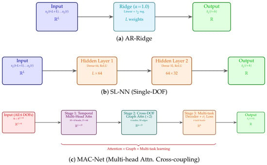
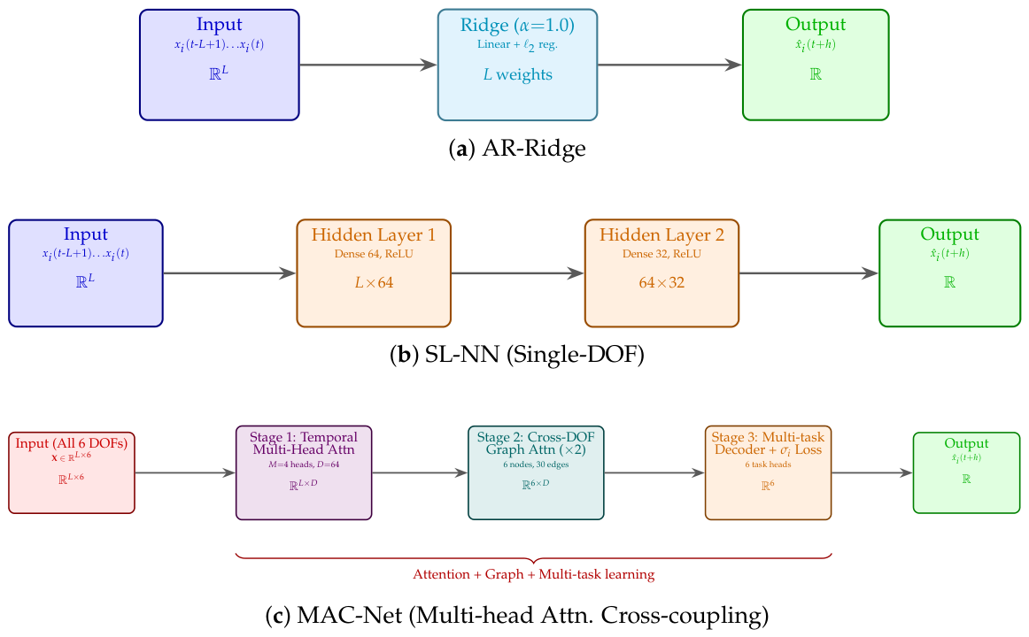
Three prediction models were evaluated, representing increasing levels of complexity. Figure 2 shows the three architectures.

3.3.1. Autoregressive Model (AR)

The autoregressive model is the simplest baseline. For each DOF $x_i$, the prediction is a linear combination of the past L values:

$${\widehat{x}}_i(t+h)={\displaystyle \sum _{k=1}^L}{w}_k{x}_i(t-L+k)$$

(4)

where $w_k$ are the regression coefficients. In matrix notation, Equation (4) can be written as:

$${\widehat{x}}_i={\mathbf{w}}^{\top }{\mathbf{z}}_i$$

(5)

where $\mathbf{w}={[w_1,w_2,\dots ,w_L]}^{\top }$ is the weight vector and ${\mathbf{z}}_i$ is the input vector defined in Equation (1).

The ordinary least squares (OLS) solution minimizes the sum of squared residuals:

$${\mathbf{w}}_{\mathrm{OLS}}={\left({\mathbf{Z}}^{\top }\mathbf{Z}\right)}^{-1}{\mathbf{Z}}^{\top }\mathbf{y}$$

(6)

where $\mathbf{Z}\in {\mathbb{R}}^{N_{\mathrm{tr}}\times L}$ is the design matrix formed by stacking all training input vectors, and $\mathbf{y}\in {\mathbb{R}}^{N_{\mathrm{tr}}}$ is the corresponding vector of target values.

To prevent overfitting and improve numerical stability, ridge regression (Tikhonov regularization) [26] was used. The regularized objective adds an ${\mathsf{\ell }}_2$ penalty on the weight magnitudes:

$${\mathcal{L}}_{\mathrm{ridge}}\left(\mathbf{w}\right)={\parallel \mathbf{y}-\mathbf{Z}\mathbf{w}\parallel }^2+\alpha {\parallel \mathbf{w}\parallel }^2$$

(7)

where $\alpha >0$ is the regularization parameter. The closed-form solution is:

$${\mathbf{w}}_{\mathrm{ridge}}={({\mathbf{Z}}^{\top }\mathbf{Z}+\alpha \mathbf{I})}^{-1}{\mathbf{Z}}^{\top }\mathbf{y}$$

(8)

In this study, $\alpha =1.0$ was selected based on cross-validation. The AR model treats each degree of freedom independently and captures only the temporal autocorrelation within each motion channel.

3.3.2. Single-DOF Neural Network (SL-NN)

The second model represents the class of standard neural network approaches that process each DOF independently. A multi-layer perceptron (MLP) [27] with two hidden layers was used to capture nonlinear temporal dependencies. The input is the past L values of a single DOF, and the output is the predicted value at horizon h.

For a network with two hidden layers, the forward pass is expressed as:

$$\begin{array}{cc}\hfill {\mathbf{h}}^{\left(1\right)}& =\varphi \left({\mathbf{W}}^{\left(1\right)}{\mathbf{z}}_i+{\mathbf{b}}^{\left(1\right)}\right)\hfill \end{array}$$

(9)

$$\begin{array}{cc}\hfill {\mathbf{h}}^{\left(2\right)}& =\varphi \left({\mathbf{W}}^{\left(2\right)}{\mathbf{h}}^{\left(1\right)}+{\mathbf{b}}^{\left(2\right)}\right)\hfill \end{array}$$

(10)

$$\begin{array}{cc}\hfill {\widehat{x}}_i(t+h)& ={\mathbf{w}}^{\left(3\right)\top }{\mathbf{h}}^{\left(2\right)}+b^{\left(3\right)}\hfill \end{array}$$

(11)

where ${\mathbf{W}}^{\left(1\right)}\in {\mathbb{R}}^{n_1\times L}$ and ${\mathbf{W}}^{\left(2\right)}\in {\mathbb{R}}^{n_2\times n_1}$ are the weight matrices of the first and second hidden layers, $n_1=64$ and $n_2=32$ are the numbers of neurons, and $\varphi$ denotes the elementwise activation function. The Rectified Linear Unit (ReLU) activation function was used:

$$\varphi \left(a\right)=max(0,a)$$

(12)

ReLU was chosen for its computational efficiency and its ability to mitigate the vanishing gradient problem [27]. The network parameters $\mathit{\theta }=\{{\mathbf{W}}^{\left(1\right)},{\mathbf{b}}^{\left(1\right)},{\mathbf{W}}^{\left(2\right)},{\mathbf{b}}^{\left(2\right)},{\mathbf{w}}^{\left(3\right)},b^{\left(3\right)}\}$ were optimized by minimizing the mean squared error (MSE):

$$\mathcal{L}\left(\mathit{\theta }\right)={\displaystyle \frac{1}{N_{\mathrm{tr}}}}{\displaystyle \sum _{j=1}^{N_{\mathrm{tr}}}}{\left(x_j-{\widehat{x}}_j\left(\mathit{\theta }\right)\right)}^2$$

(13)

using the Adam optimizer, which maintains adaptive estimates of the first and second moments of the gradients:

$$\begin{array}{cc}\hfill {\mathbf{m}}_t& ={\beta }_1{\mathbf{m}}_{t-1}+(1-{\beta }_1){\nabla }_{\mathit{\theta }}{\mathcal{L}}_t\hfill \end{array}$$

(14)

$$\begin{array}{cc}\hfill {\mathbf{v}}_t& ={\beta }_2{\mathbf{v}}_{t-1}+(1-{\beta }_2){\left({\nabla }_{\mathit{\theta }}{\mathcal{L}}_t\right)}^2\hfill \end{array}$$

(15)

$$\begin{array}{cc}\hfill {\mathit{\theta }}_t& ={\mathit{\theta }}_{t-1}-{\displaystyle \frac{\eta }{\sqrt{{\widehat{\mathbf{v}}}_t}+ϵ}}{\widehat{\mathbf{m}}}_t\hfill \end{array}$$

(16)

where ${\widehat{\mathbf{m}}}_t={\mathbf{m}}_t/(1-{\beta }_1^t)$ and ${\widehat{\mathbf{v}}}_t={\mathbf{v}}_t/(1-{\beta }_2^t)$ are bias-corrected estimates. The hyperparameters were set to ${\beta }_1=0.9$, ${\beta }_2=0.999$, $ϵ={10}^{-8}$, and learning rate $\eta ={10}^{-3}$. Early stopping with a patience of 20 epochs on a 15% validation split was used to prevent overfitting.

3.3.3. Multi-Head Attention Cross-Coupling Network (MAC-Net)

The third model, which is the main contribution of this study, exploits cross-coupling among all six DOFs through a three-stage architecture: temporal attention encoding, cross-DOF graph message passing, and multi-task decoding with uncertainty-weighted loss. The physical motivation is that the motions of a moored vessel are coupled through the hull geometry, the mooring system, and the environmental loading [13]. Surge motions induced by wave drift forces, for instance, are transmitted through the turret mooring system to the vessel roll response.

Stage 1: Temporal Attention Encoding

Rather than feeding the flattened input directly into dense layers, MAC-Net first reshapes the input into a matrix $\mathbf{X}\in {\mathbb{R}}^{L\times 6}$ and applies multi-head self-attention along the temporal dimension to capture long-range dependencies. Positional encoding is added to inject temporal order:

$${\mathbf{E}}_{\mathrm{pos}}(l,2d)=sin\left(l/{10000}^{2d/D}\right),{\mathbf{E}}_{\mathrm{pos}}(l,2d+1)=cos\left(l/{10000}^{2d/D}\right)$$

(17)

where $l=1,\dots ,L$ is the time step index, $d=0,1,\dots ,D/2-1$, and $D=64$ is the embedding dimension per DOF. The attention input is ${\mathbf{H}}^{\left(0\right)}=\mathbf{X}{\mathbf{W}}_E+{\mathbf{E}}_{\mathrm{pos}}\in {\mathbb{R}}^{L\times D}$.

The scaled dot-product attention computes query, key, and value projections:

$$\mathrm{Attn}(\mathbf{Q},\mathbf{K},\mathbf{V})=\mathrm{softmax}\left({\displaystyle \frac{\mathbf{Q}{\mathbf{K}}^{\top }}{\sqrt{d_k}}}\right)\mathbf{V}$$

(18)

where $\mathbf{Q}={\mathbf{H}}^{\left(0\right)}{\mathbf{W}}_Q$, $\mathbf{K}={\mathbf{H}}^{\left(0\right)}{\mathbf{W}}_K$, $\mathbf{V}={\mathbf{H}}^{\left(0\right)}{\mathbf{W}}_V$, with ${\mathbf{W}}_Q,{\mathbf{W}}_K\in {\mathbb{R}}^{D\times d_k}$ and ${\mathbf{W}}_V\in {\mathbb{R}}^{D\times d_v}$. Multi-head attention with M heads extends this by concatenating the outputs of M parallel attention functions:

$$\mathrm{MultiHead}\left({\mathbf{H}}^{\left(0\right)}\right)=\mathrm{Concat}({\mathrm{head}}_1,\dots ,{\mathrm{head}}_M){\mathbf{W}}_O$$

(19)

where ${\mathrm{head}}_m=\mathrm{Attn}({\mathbf{H}}^{\left(0\right)}{\mathbf{W}}_Q^{\left(m\right)},{\mathbf{H}}^{\left(0\right)}{\mathbf{W}}_K^{\left(m\right)},{\mathbf{H}}^{\left(0\right)}{\mathbf{W}}_V^{\left(m\right)})$ and ${\mathbf{W}}_O\in {\mathbb{R}}^{M{d}_v\times D}$. In this study, $M=4$, $d_k=d_v=D/M=16$.

A residual connection and layer normalization are applied after the multi-head attention:

$${\overline{\mathbf{H}}}^{\left(1\right)}=\mathrm{LayerNorm}\left({\mathbf{H}}^{\left(0\right)}+\mathrm{MultiHead}\left({\mathbf{H}}^{\left(0\right)}\right)\right)$$

(20)

followed by a position-wise feed-forward network with GELU activation:

$${\mathbf{H}}^{\left(1\right)}=\mathrm{LayerNorm}\left({\overline{\mathbf{H}}}^{\left(1\right)}+\mathrm{FFN}({\overline{\mathbf{H}}}^{\left(1\right)})\right),\mathrm{FFN}\left(\mathbf{x}\right)={\mathbf{W}}_2\mathrm{GELU}({\mathbf{W}}_1\mathbf{x}+{\mathbf{b}}_1)+{\mathbf{b}}_2$$

(21)

where ${\mathbf{W}}_1\in {\mathbb{R}}^{D\times 4D}$, ${\mathbf{W}}_2\in {\mathbb{R}}^{4D\times D}$, and the GELU activation is defined as $\mathrm{GELU}\left(x\right)=x\Phi \left(x\right)$ with $\Phi (·)$ being the standard Gaussian CDF. The output ${\mathbf{H}}^{\left(1\right)}\in {\mathbb{R}}^{L\times D}$ is then aggregated across time by averaging to obtain a DOF-level representation:

$${\mathbf{h}}_i^{\mathrm{temp}}={\displaystyle \frac{1}{L}}{\displaystyle \sum _{l=1}^L}{\mathbf{H}}_{l,:}^{\left(1\right)}\odot {\mathbf{m}}_i\in {\mathbb{R}}^D$$

(22)

where ${\mathbf{m}}_i\in {\{0,1\}}^D$ is a DOF-specific mask that selects the features corresponding to the i-th degree of freedom from the concatenated embedding.

Stage 2: Cross-DOF Graph Message Passing

The six DOFs are represented as nodes in a fully connected graph $\mathcal{G}=(\mathcal{V},\mathcal{E})$, where $\left|\mathcal{V}\right|=6$ and $\left|\mathcal{E}\right|=30$ (each pair of DOFs is connected in both directions). Each node i has an initial feature vector ${\mathbf{h}}_i^{\left(0\right)}={\mathbf{h}}_i^{\mathrm{temp}}$ from the temporal attention stage. A graph attention network (GAT) [28] is used to learn the coupling weights between DOFs.

For an edge $(i\to j)\in \mathcal{E}$, the attention coefficient is computed as:

$$e_{ij}=\mathrm{LeakyReLU}\left({\mathbf{a}}^{\top }[{\mathbf{W}}_g{\mathbf{h}}_i^{\left(0\right)}\parallel {\mathbf{W}}_g{\mathbf{h}}_j^{\left(0\right)}]\right)$$

(23)

where ${\mathbf{W}}_g\in {\mathbb{R}}^{D^{\prime }\times D}$ is a shared linear transformation, $\mathbf{a}\in {\mathbb{R}}^{2D^{\prime }}$ is a learnable attention vector, and ∥ denotes concatenation. The coefficients are normalized via softmax over all incoming edges to node j:

$${\alpha }_{ij}={\displaystyle \frac{exp\left(e_{ij}\right)}{{\sum }_{k\in \mathcal{N}\left(j\right)}exp\left(e_{kj}\right)}}$$

(24)

The message passing update for node j aggregates information from all neighbors:

$${\mathbf{h}}_j^{\left(1\right)}=\sigma \left(\sum _{i\in \mathcal{N}\left(j\right)}{\alpha }_{ij}{\mathbf{W}}_g{\mathbf{h}}_i^{\left(0\right)}\right)$$

(25)

where $\sigma$ denotes the ELU activation. Two layers of graph attention are applied with residual connections:

$${\mathbf{h}}_j^{\left(2\right)}=\sigma \left(\sum _{i\in \mathcal{N}\left(j\right)}{\alpha }_{ij}^{\left(2\right)}{\mathbf{W}}_g^{\left(2\right)}{\mathbf{h}}_i^{\left(1\right)}\right)+{\mathbf{h}}_j^{\left(0\right)}$$

(26)

This mechanism allows each DOF to receive weighted information from all other DOFs, with the attention weights ${\alpha }_{ij}$ learning the physical coupling strength between degrees of freedom.

Stage 3: Multi-Task Decoding with Uncertainty-Weighted Loss

The final DOF representations ${\mathbf{h}}_j^{\left(2\right)}\in {\mathbb{R}}^D$ are passed through task-specific decoder heads, each consisting of two fully connected layers with residual skip connections:

$$\begin{array}{cc}\hfill {\mathbf{d}}_i^{\left(1\right)}& =\mathrm{GELU}\left({\mathbf{U}}_i^{\left(1\right)}{\mathbf{h}}_i^{\left(2\right)}+{\mathbf{c}}_i^{\left(1\right)}\right)+{\mathbf{h}}_i^{\left(2\right)}\hfill \end{array}$$

(27)

$$\begin{array}{cc}\hfill {\widehat{x}}_i(t+h)& ={\mathbf{u}}_i^{\left(2\right)\top }{\mathbf{d}}_i^{\left(1\right)}+c_i^{\left(2\right)}\hfill \end{array}$$

(28)

where ${\mathbf{U}}_i^{\left(1\right)}\in {\mathbb{R}}^{D\times D}$ and the residual connection ensures gradient flow.

Since the six prediction tasks involve motion quantities of different magnitudes and physical units (cm for translations, degrees for rotations), a multi-task learning framework with homoscedastic uncertainty weighting [29] is adopted. Each task i is assigned a learnable noise parameter ${\sigma }_i>0$, and the combined loss is:

$${\mathcal{L}}_{\mathrm{MT}}={\displaystyle \sum _{i=1}^6}{\displaystyle \frac{1}{2{\sigma }_i^2}}{\mathcal{L}}_i\left({\mathit{\theta }}_i\right)+ln{\sigma }_i$$

(29)

where ${\mathcal{L}}_i$ is the MSE loss for the i-th DOF defined in Equation (13), and the $ln{\sigma }_i$ term prevents the network from assigning infinite variance to any task. The noise parameters $\{{\sigma }_1,\dots ,{\sigma }_6\}$ are optimized jointly with the network weights. Tasks with higher inherent noise (e.g., heave, pitch) are automatically assigned larger ${\sigma }_i$ and thus lower weight in the loss, while well-predictable tasks (e.g., surge, yaw) receive higher relative weight.

Implementation Details

The complete MAC-Net architecture contains approximately 85,000 trainable parameters. The temporal attention module with four heads contributes $4\times (D\times d_k+D\times d_k+D\times d_v)+D\times D\approx 33,000$ parameters; the two-layer GAT with $D^{\prime }=32$ contributes $2\times (D^{\prime }\times D+2D^{\prime }+D^{\prime }\times D)\approx 8000$ parameters; the six decoder heads contribute $6\times (D^2+D)\approx 25,000$ parameters; and the remainder comes from positional encoding, layer normalization, and the FFN sub-layers. The model was trained using the AdamW optimizer with weight decay $\lambda =0.01$, learning rate $\eta =5\times {10}^{-4}$, and a cosine annealing schedule. Dropout with rate $p=0.1$ was applied to the attention weights and the FFN sub-layers. Early stopping with a patience of 30 epochs on a 15% validation split was used to prevent overfitting.

3.4. Evaluation Metrics

Three metrics were used to evaluate prediction performance:

• Root mean square error (RMSE):

  $$\mathrm{RMSE}=\sqrt{{\displaystyle \frac{1}{N}}\sum _{j=1}^N{\left(x_j-{\widehat{x}}_j\right)}^2}$$

  (30)
• Mean absolute error (MAE):

  $$\mathrm{MAE}={\displaystyle \frac{1}{N}}{\displaystyle \sum _{j=1}^N}|x_j-{\widehat{x}}_j|$$

  (31)
• Skill score (SS), defined as the Nash–Sutcliffe efficiency [30]:

  $$\mathrm{SS}=1-{\displaystyle \frac{{\sum }_{j=1}^N{(x_j-{\widehat{x}}_j)}^2}{{\sum }_{j=1}^N{(x_j-\overline{x})}^2}}$$

  (32)

  where $\overline{x}$ is the mean of the observed values. A skill score of 1.0 indicates a perfect prediction, 0.0 means the prediction is no better than using the mean, and negative values indicate worse-than-mean performance.

3.5. Collision Risk Assessment

For the side-by-side offloading cases, the relative motions between the FLNG and the LNGC were computed to assess collision risk. The relative surge ($\Delta u$), relative sway ($\Delta v$), and relative yaw ($\Delta \psi$) were obtained by subtracting the LNGC motions from the FLNG motions at each time step:

$$\begin{array}{cc}\hfill \Delta u\left(t\right)& =u_{\mathrm{FLNG}}\left(t\right)-u_{\mathrm{LNGC}}\left(t\right)\hfill \end{array}$$

(33)

$$\begin{array}{cc}\hfill \Delta v\left(t\right)& =v_{\mathrm{FLNG}}\left(t\right)-v_{\mathrm{LNGC}}\left(t\right)\hfill \end{array}$$

(34)

$$\begin{array}{cc}\hfill \Delta \psi \left(t\right)& ={\psi }_{\mathrm{FLNG}}\left(t\right)-{\psi }_{\mathrm{LNGC}}\left(t\right)\hfill \end{array}$$

(35)

The relative lateral clearance at the midship position can be approximated as:

$$d_{\mathrm{gap}}\left(t\right)=d_0+\Delta v\left(t\right)+{\displaystyle \frac{L_{\mathrm{FLNG}}}{2}}sin\left(\Delta \psi \left(t\right)\right)+{\displaystyle \frac{L_{\mathrm{LNGC}}}{2}}sin\left(\Delta \psi \left(t\right)\right)$$

(36)

where $d_0$ is the static gap distance. The predicted clearance is obtained by substituting the predicted relative motions into Equation (36):

$${\widehat{d}}_{\mathrm{gap}}(t+h)=d_0+\widehat{\Delta v}(t+h)+{\displaystyle \frac{L_{\mathrm{FLNG}}+L_{\mathrm{LNGC}}}{2}}sin\left(\widehat{\Delta \psi }(t+h)\right)$$

(37)

A warning signal is triggered when the predicted gap falls below a safety threshold ${\delta }_{min}$, corresponding to the allowable fender compression:

$$\mathcal{A}\left(t\right)=\left\{\begin{array}{cc}1,\hfill & {\widehat{d}}_{\mathrm{gap}}(t+h)<{\delta }_{min}\hfill \\ 0,\hfill & \mathrm{otherwise}\hfill \end{array}\right.$$

(38)

In an engineering implementation, $d_0$ and ${\delta }_{min}$ must be set from the actual offloading arrangement, including the nominal hull gap, fender load–deflection curve, loading-arm operating envelope, and any project-specific clearance margin. In this paper the framework is therefore used as a conversion from predicted relative motions to a warning index rather than as a certified alarm limit. For example, DL25 represents an in-line operating case for checking normal transfer conditions, whereas DL27 represents a quartering-sea operating case in which relative sway and yaw are larger and the predicted value of Equation (37) would be expected to approach the allowable envelope earlier. A practical deployment would issue a caution alarm when ${\widehat{d}}_{\mathrm{gap}}$ approaches ${\delta }_{min}$ at the 4 s model-scale horizon (32 s full-scale equivalent) and an action alarm when the exceedance persists or is predicted at the 1–2 s model-scale horizon.

4. Results and Discussion

4.1. Motion Response Characteristics

4.1.1. Time-Series Overview

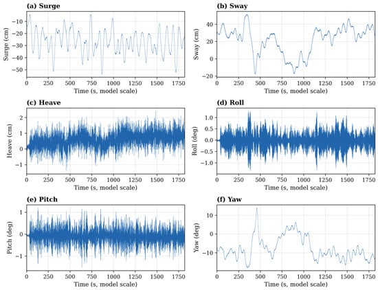
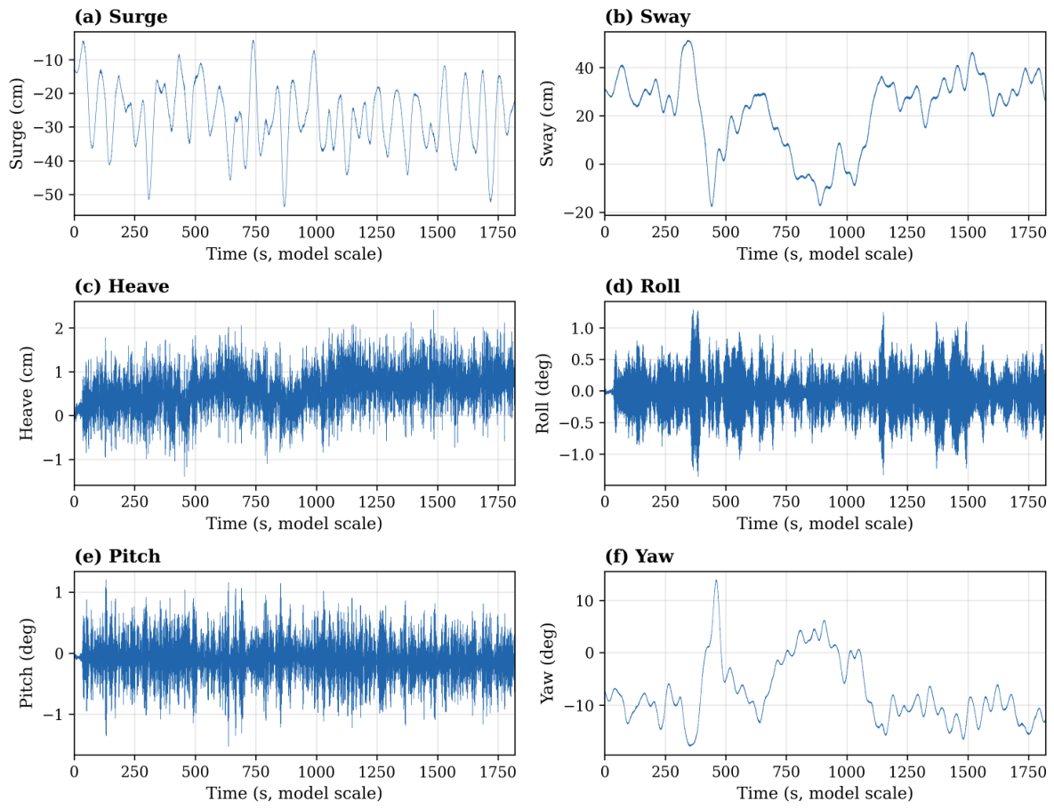
Figure 3 presents the measured six-DOF motion responses of the FLNG vessel under the combined 100-year return period condition DL14 (full load, in-line), shown in model-scale units (cm for translations, degrees for rotations). The time-series span approximately 1800 s in the model scale. Surge and sway exhibit low-frequency drift superimposed on higher-frequency oscillations, with surge showing a mean offset of approximately $-27$ cm (drift downwind) and sway fluctuating around a near-zero mean. Yaw also displays a low-frequency component, with the vessel oscillating around a mean heading offset of about $-7.6$ degrees. Heave, roll, and pitch are dominated by wave-frequency responses, with negligible mean offsets.

4.1.2. Comparison Across Environmental Conditions

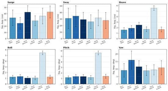
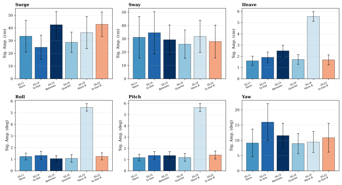
Figure 4 compares the significant amplitudes of each DOF across six selected test conditions (model-scale values). Wave-only conditions (DL11 for full load, DL19 for ballast) produce substantial surge motions (significant amplitudes of approximately 33 cm and 36 cm, respectively, in the model scale) due to second-order wave drift forces. Adding wind and current (DL14, DL22) increases the mean drift but slightly reduces the oscillatory component as the mooring system reaches a more offset equilibrium position with higher stiffness.

Table 3. FLNG motion significant amplitudes under 100-year return period conditions (model scale).

Condition	Surge (cm)	Sway (cm)	Heave (cm)	Roll (°)	Pitch (°)	Yaw (°)
Full Load
DL11	33.494	31.114	1.594	1.235	1.177	9.148
DL14	24.758	34.563	1.906	1.322	1.366	15.967
DL15	42.516	29.317	2.488	1.049	1.359	11.543
DL16	28.741	26.017	1.716	1.070	1.192	8.946
Ballast
DL19	36.324	31.794	5.551	5.458	5.623	9.450
DL22	42.888	27.959	1.686	1.245	1.410	10.863
DL23	54.182	34.037	5.650	5.879	5.717	10.498
DL24	43.848	68.188	5.730	5.758	5.672	22.106

lists the corresponding significant amplitudes for the 100-year return period cases, confirming that ballast loading substantially amplifies angular responses, whereas the largest horizontal-plane responses depend on heading and environmental combination.

The between-line condition (DL15) produces the largest surge drift (approximately 42 cm significant amplitude in model scale) because the environmental forces are applied perpendicular to a mooring group, resulting in less restoring force in the surge direction. The quartering conditions (DL16, DL24) generate the largest yaw motions (up to approximately 22 degrees for DL24 in ballast) as the asymmetric loading induces a weathervaning torque about the turret.

Roll and pitch responses are markedly larger in ballast conditions (up to 5.9 degrees significant roll amplitude) than in full load (up to 1.3 degrees). This is attributable to the higher center of gravity and larger metacentric height in ballast, which amplify the angular motions.

4.1.3. Effect of Loading Condition

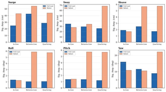
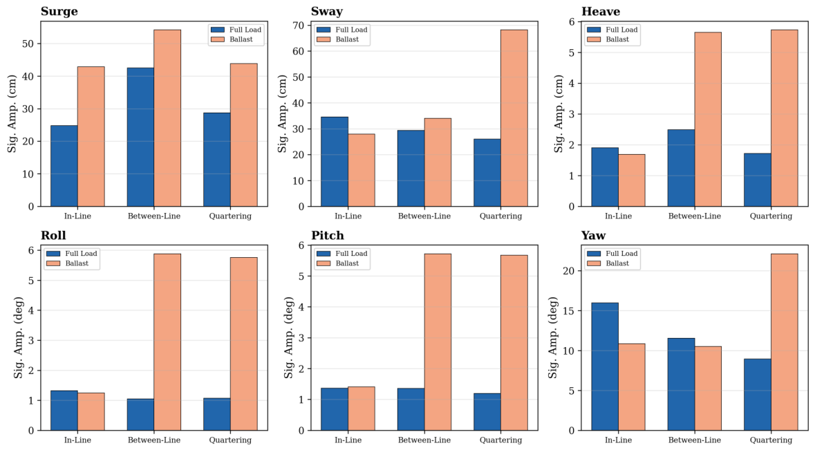
Figure 5 directly compares the motion significant amplitudes between full load and ballast for the same environmental heading. Ballast consistently produces larger angular motions (roll and pitch) due to the reduced draft and higher natural roll period. For linear motions (surge, sway), the differences depend on the heading: ballast produces larger surge amplitudes under both in-line (DL22 vs. DL14) and between-line (DL23 vs. DL15) conditions due to the reduced draft and lower hydrostatic restoring force, while sway shows the opposite trend under in-line conditions (DL22 vs. DL14).

4.1.4. Power Spectral Density Analysis

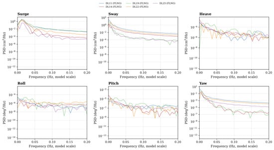
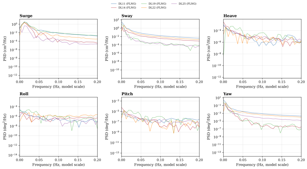
Figure 6 shows the power spectral density (PSD) of the FLNG motions for selected conditions. The surge and sway spectra are dominated by low-frequency energy below 0.05 Hz, corresponding to the slowly varying drift response, with a secondary peak near the wave spectral peak at 0.07 Hz (14.2 s period). The yaw spectrum shows a similar bimodal structure. In contrast, the heave, roll, and pitch spectra are concentrated around the wave-frequency range (0.04–0.12 Hz), with peak frequencies close to the wave spectral peak.

The spectral characteristics have direct implications for predictability: motions with strong low-frequency components (surge, sway, yaw) have higher temporal autocorrelation and are therefore more amenable to short-term prediction, while wave-frequency motions (heave, pitch) are more stochastic and reach their predictability limit sooner.

4.1.5. Motion Distributions

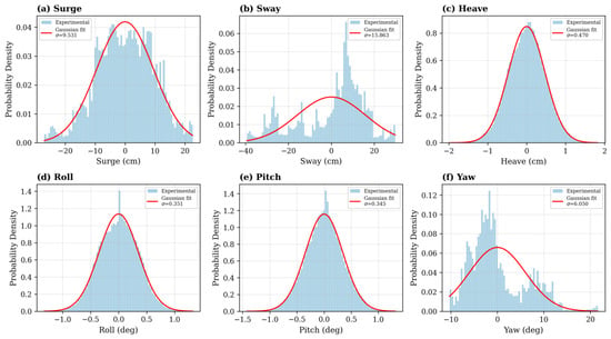
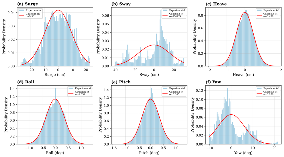
Figure 7 shows the probability distributions of the FLNG motions under the DL14 condition. The translational motions (surge, sway, heave) follow approximately Gaussian distributions after mean removal, as indicated by the close agreement between the experimental histogram and the fitted Gaussian curve. The angular motions (roll, pitch, yaw) also show near-Gaussian behavior, with roll and pitch being slightly more peaked than Gaussian. This near-Gaussian character validates the use of standard deviation-based thresholds for collision risk assessment.

4.2. Prediction Performance

The prediction models were trained and evaluated on the DL14 condition (combined environmental loads, full load, in-line heading) as a representative test case. The lookback window was set to 50 samples (10 s at 5 Hz in the model scale, equivalent to 80 s full scale), and five model-scale prediction horizons were tested: 0.2, 1.0, 2.0, 4.0, and 10.0 s. The corresponding full-scale lead times are 1.6, 8, 16, 32, and 80 s.

4.2.1. Overall Comparison

Table 4. Prediction skill scores for all degrees of freedom and horizons (DL14, full load).

DOF	Method	0.2 s	1.0 s	2.0 s	4.0 s	10.0 s
Surge	AR	0.9997	0.9993	0.9984	0.9927	0.9143
	SL-NN	0.9989	0.9978	0.9958	0.9843	0.8461
	MAC-Net	0.9925	0.9911	0.9837	0.9635	0.7128
Sway	AR	0.9991	0.9989	0.9980	0.9944	0.9476
	SL-NN	0.9967	0.9952	0.9964	0.9914	0.9285
	MAC-Net	0.9275	0.9260	0.8954	0.8975	0.6706
Heave	AR	0.8379	0.6410	0.2828	0.1161	0.0139
	SL-NN	0.8104	0.5876	0.2021	0.0819	−0.0352
	MAC-Net	0.7703	0.4389	−0.3735	−0.6667	−1.0031
Roll	AR	0.9854	0.9639	0.9108	0.7581	0.5134
	SL-NN	0.9818	0.9587	0.8996	0.7351	0.4691
	MAC-Net	0.9749	0.9573	0.9408	0.8819	0.2019
Pitch	AR	0.9670	0.8505	0.5662	0.0952	−0.0146
	SL-NN	0.9539	0.8181	0.4705	−0.0494	−0.0693
	MAC-Net	0.9101	0.7224	0.1252	−1.1168	−1.2255
Yaw	AR	0.9994	0.9993	0.9982	0.9943	0.9306
	SL-NN	0.9966	0.9974	0.9959	0.9897	0.9170
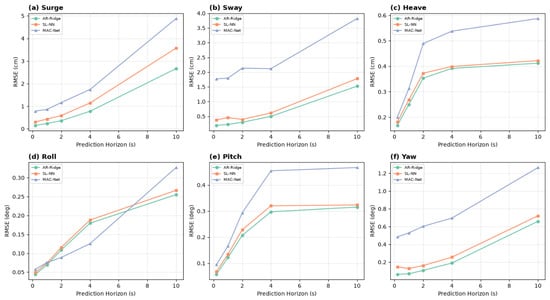
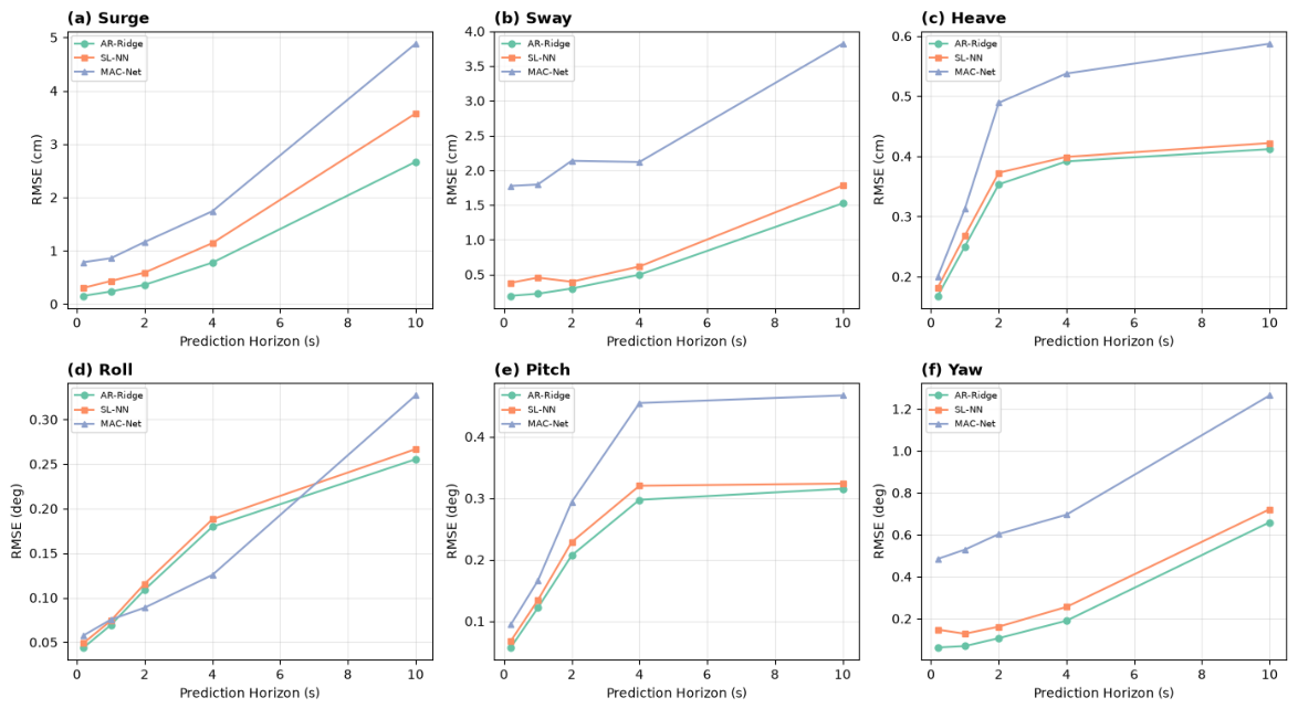
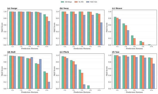
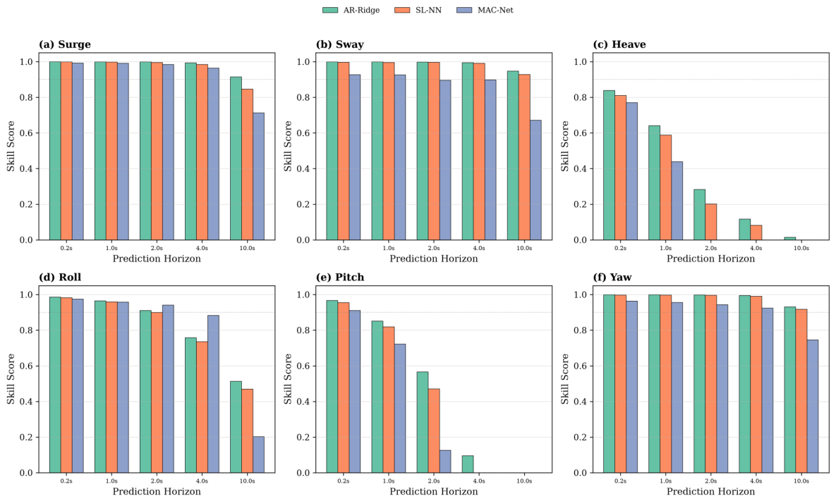
	MAC-Net	0.9630	0.9559	0.9426	0.9236	0.7451

summarizes the skill scores for all three models across all six degrees of freedom and prediction horizons.

Table 5. Model complexity and recommended use based on the DL14 same-condition results.

Model	Approx. Parameters	Main Advantage	Recommended Use
AR-Ridge	∼50 per DOF	Highest interpretability and low computational cost	First choice for surge, sway, and yaw when the sea state is close to the calibrated condition and transparent warning logic is required.
SL-NN	∼5300 per DOF	Simple nonlinear single-DOF mapping	Useful as a nonlinear baseline, but it did not consistently outperform AR-Ridge in the present tests.
MAC-Net	∼85,000 total	Uses temporal attention, cross-DOF graph coupling, and multi-task learning	Recommended when coupled motions are important, especially roll prediction and side-by-side relative motion monitoring. It is less suitable for heave and pitch at long horizons unless additional wave inputs are available.

shows the model complexity and recommended use based on the DL14 same-condition results. Figure 8 presents the RMSE as a function of prediction horizon, and Figure 9 provides a bar chart comparison of skill scores.

The main findings are as follows:

• Surge, sway, and yaw can be predicted with high accuracy at short horizons. The AR model achieves skill scores above 0.99 for surge and yaw at 2 s ahead, and above 0.94 at 10 s ahead for yaw. These motions are dominated by low-frequency drift and slowly varying components that exhibit strong temporal autocorrelation.
• Heave and pitch are considerably less predictable. The AR model achieves skill scores below 0.3 at 2 s ahead for heave and pitch. These motions are primarily driven by wave-frequency excitation, which becomes decorrelated from the past values beyond approximately one wave period (14.2 s). At very short horizons (0.2 s), the autocorrelation is still high (skill score 0.84 for heave), but it drops rapidly as the horizon increases.
• Roll shows an intermediate level of predictability, with skill scores of 0.91 (AR model) at 2 s ahead. The MAC-Net model improves this to 0.94 at 2 s and 0.88 at 4 s, substantially outperforming both the AR model (0.76) and the SL-NN model (0.74) at the 4 s horizon.

4.2.2. Advantage of Multi-DOF Approach for Roll

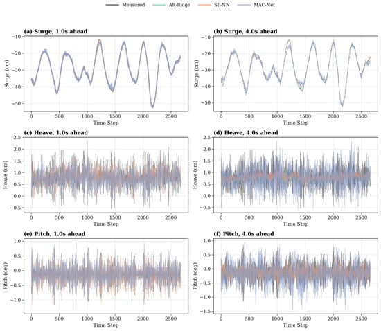
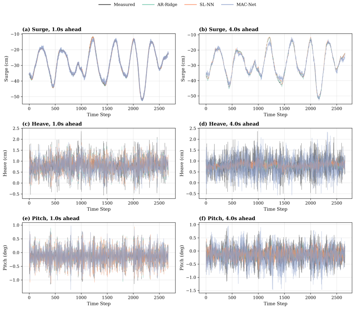
The most notable result is the improvement achieved by the MAC-Net model for roll prediction. At the 4 s horizon, the MAC-Net model achieves a skill score of 0.88, compared to 0.76 for the AR model and 0.74 for the SL-NN model (as shown in Figure 10). This 16-percentage-point improvement over the conventional methods is physically attributable to the coupling between roll and the horizontal-plane motions through the turret mooring system.

When the FLNG vessel experiences surge or sway motions, the mooring lines generate restoring forces that are not applied exactly at the vessel’s center of gravity but at the turret location near the bow. The resulting moment arm induces roll excitation. The MAC-Net model, by observing all six DOFs simultaneously, can learn this coupling relationship and use the horizontal-plane motion information to improve roll predictions. The SL-NN model, which processes only the roll time history, cannot capture this coupling.

This finding has practical significance because roll is one of the critical motions for side-by-side offloading safety: large roll angles of the FLNG increase the relative motions at the cargo transfer point and can cause the loading arms to exceed their operational envelope.

4.2.3. Limitations for Heave and Pitch

The poor predictability of heave and pitch at horizons beyond 2 s is an inherent limitation of time-series-based prediction. Wave-induced heave and pitch are primarily responses to individual wave encounters, and the phase relationship between successive wave crests decorrelates over time scales comparable to the wave period. No amount of model complexity can overcome this stochastic limit. For operational purposes, heave and pitch cannot be reliably used as early warning indicators at horizons beyond 2 s. Alternative approaches, such as wave measurement-based feed-forward prediction or coupled wave–response models, would be needed for longer-horizon prediction of these motions.

4.3. Side-by-Side Offloading Analysis

4.3.1. Relative Motions

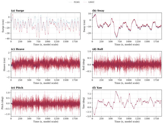
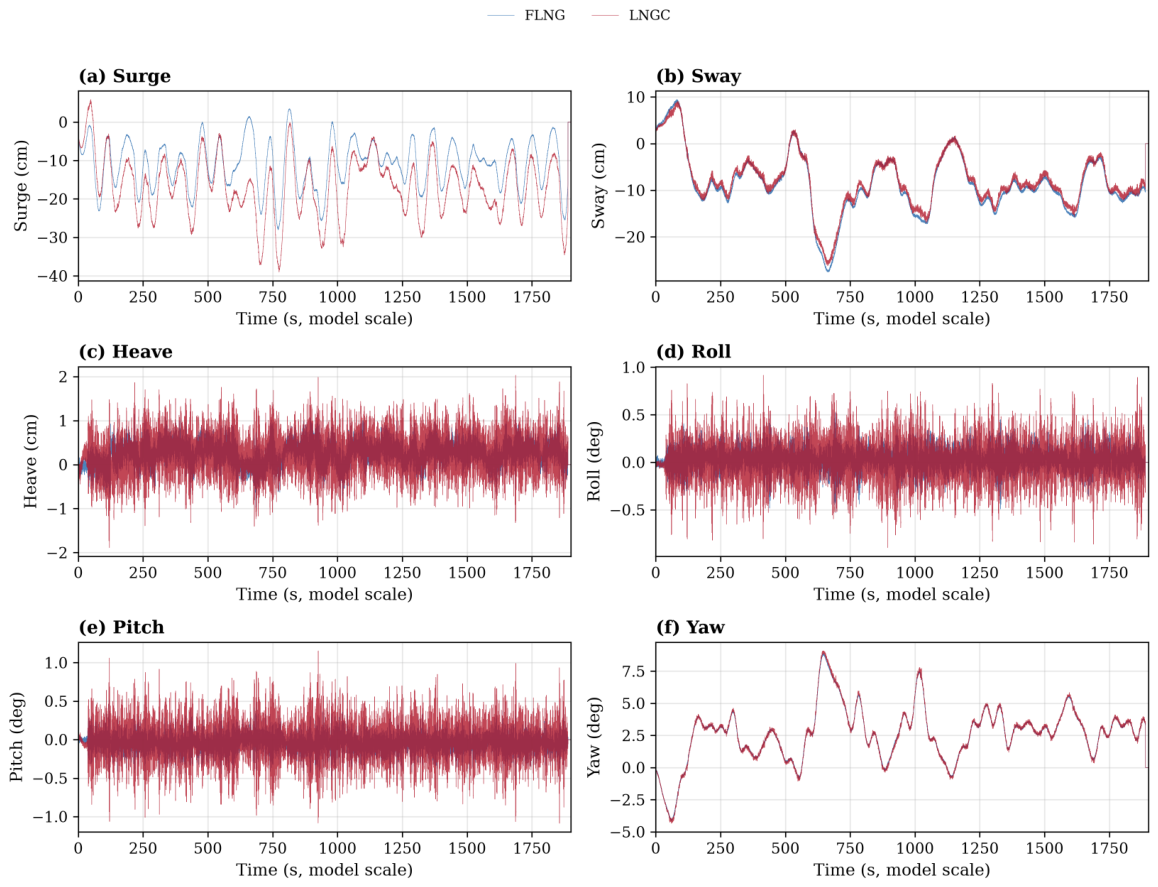
Figure 11 compares the motion time histories of the FLNG and LNGC during the side-by-side offloading condition DL25 (in-line, 1-year return period). All values are in model-scale units. The LNGC generally exhibits slightly larger amplitudes than the FLNG in heave and pitch, due to its smaller size and lower inertia, while the two vessels show similar horizontal-plane motion patterns because they are connected through the hawser system.

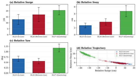
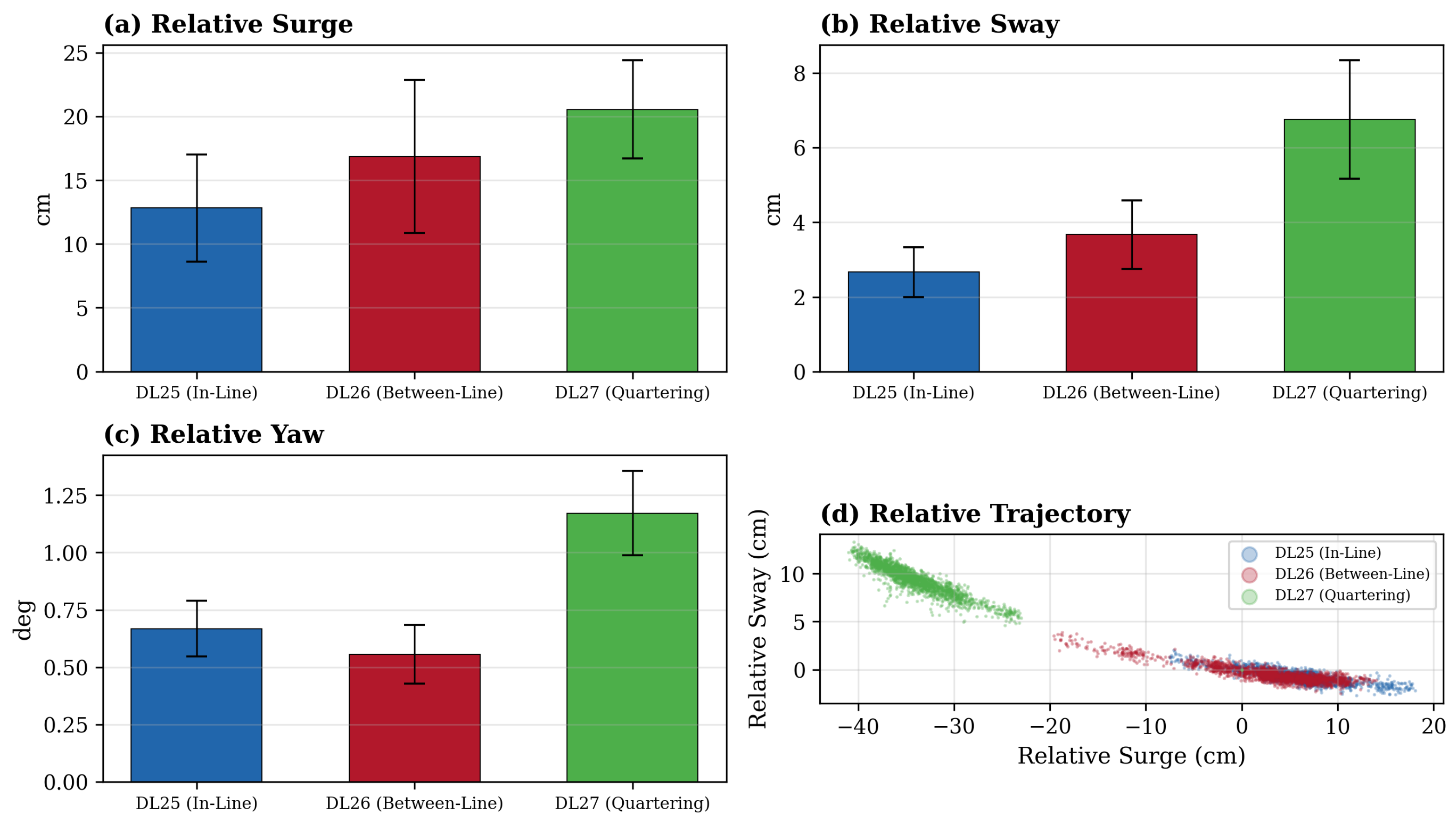
Figure 12 presents the relative motions between the two vessels for the three side-by-side conditions. The between-line condition (DL26) produces the largest relative surge (approximately 29 cm significant amplitude in the model scale), while the quartering condition (DL27) produces the largest relative sway and relative yaw. The relative trajectory scatter plots in Figure 12d show that the between-line and quartering conditions produce wider distributions of relative horizontal positions, indicating a larger collision envelope.

4.3.2. Prediction During Side-by-Side Operations

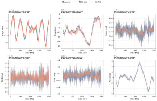
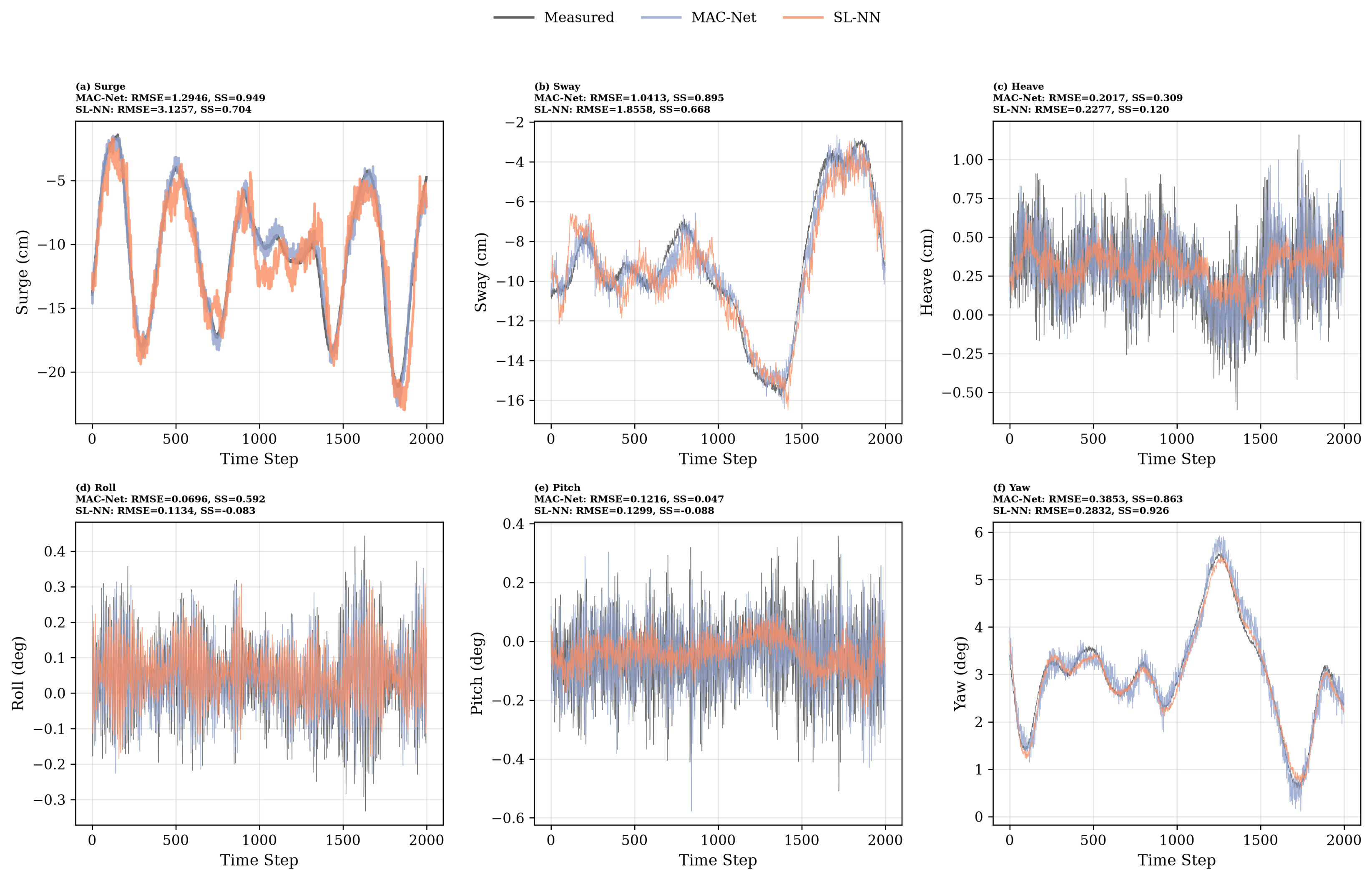
Figure 13 shows the prediction results for the side-by-side condition DL25 at a 2 s model-scale horizon. The MAC-Net model maintains skill scores above 0.95 for surge and yaw, confirming that the prediction approach applies to the side-by-side configuration. The roll prediction also achieves a high skill score (0.94), which is relevant for monitoring the relative roll between the two vessels at the cargo transfer point. These results should be interpreted as same-condition validation for an in-line operating case. A full cross-condition transfer test, for example, training on DL14 and applying the model directly to DL22, DL15, or DL16 without retraining, was not included in the present experimental evaluation. Such cross-condition validation is required before the model can be deployed as a robust general-purpose predictor under changed heading, loading, or environmental severity.

4.4. Discussion

The results presented in this study have several practical implications for the design of early warning systems for FLNG offloading operations.

First, the high predictability of surge, sway, and yaw at model-scale horizons of 4–10 s means that collision-relevant horizontal-plane motions can be forecast with full-scale lead times of 32–80 s. A prediction-based warning system could trigger alerts when the predicted relative motions are expected to exceed safe thresholds within this lead time, giving operators time to halt the offloading process, check hawser and fender loads, prepare loading-arm disconnection, or initiate vessel separation maneuvers. For the present side-by-side cases, DL25 can be regarded as the normal in-line operating scenario, whereas DL27 is the more demanding quartering-sea scenario because its relative sway and yaw enlarge the lateral collision envelope. In both cases, the warning quantity should be the predicted clearance or predicted loading-arm motion envelope, not the individual vessel motion alone.

Second, the improvement in roll prediction offered by the multi-DOF approach is noteworthy because roll is one of the motions most strongly affected by the vessel–vessel hydrodynamic interaction. A prediction model that can anticipate roll excursions 4–5 s in advance would enable early activation of anti-roll measures or temporary suspension of cargo transfer.

Third, the fundamental limitation in heave and pitch predictability suggests that these motions should be monitored in real time rather than used as longer-horizon warning variables. A practical system could combine short-horizon (1–2 s model scale, 8–16 s full-scale equivalent) prediction of heave and pitch with longer-horizon prediction of surge, sway, and yaw to provide a comprehensive motion monitoring and forecasting capability. Longer-horizon heave and pitch prediction would likely require additional feed-forward inputs, such as wave radar measurements, incident-wave reconstruction, or coupled wave–response models.

Several limitations of this study should be acknowledged. The AR and SL-NN baselines were intentionally selected as simple single-DOF predictors, while MAC-Net was designed to test whether temporal attention and cross-DOF graph message passing add value when physical coupling is important. The added complexity is justified mainly for coupled responses such as roll and for side-by-side operations where relative motion envelopes are the target; for surge, sway, and yaw under the present DL14 condition, the simpler AR model remains competitive and may be preferable when interpretability and computational cost are priorities. Additionally, the models were trained and tested primarily within individual environmental conditions, and the reported DL14 results should be regarded as a single-condition demonstration rather than proof of universal cross-condition robustness. Cross-condition generalization, where a model trained on one condition is applied to a different condition without retraining, is an important topic for future work. Finally, the use of basin experimental data provides controlled physical realism, but full-scale implementation will require sensor calibration, online quality control, site-specific warning thresholds, and validation against field measurements.

5. Conclusions

This study presented a data-driven approach to short-term motion prediction for an FLNG system, using experimental data from comprehensive basin model tests. The main findings are as follows:

• The experimental data from 15 test conditions, covering survival and operating scenarios with both single-vessel and side-by-side configurations, provide a detailed characterization of FLNG motion responses (model scale). The motion significant amplitudes ranged from 1.9 cm to 54.2 cm for translational degrees of freedom and from 0.5 to 22.1 degrees for angular motions, depending on the environmental condition and loading state.
• The power spectral density analysis revealed that surge, sway, and yaw are dominated by low-frequency components (below 0.05 Hz, full scale), while heave, roll, and pitch are concentrated in the wave-frequency range (0.04–0.12 Hz). This spectral separation has direct implications for predictability.
• Surge, sway, and yaw can be predicted with high accuracy at model-scale horizons of up to 4 s (32 s full-scale equivalent), with skill scores above 0.93 for surge and yaw. Even at the 10 s model scale, the skill score for yaw remains above 0.92, suggesting that these motions retain sufficient temporal autocorrelation for practical early warning.
• Heave and pitch exhibit limited predictability beyond 2 s (skill scores below 0.3), which is an inherent limitation of wave-induced motions whose phase decorrelates over time scales comparable to the wave period.
• The multi-head attention cross-coupling network (MAC-Net) substantially improves roll prediction compared to single-degree-of-freedom approaches, achieving a skill score of 0.88 at a 4 s model-scale horizon compared to 0.74–0.76 for the baseline methods. This improvement is physically explained by the coupling between horizontal-plane motions and roll through the turret mooring system.
• The relative motions between the FLNG and LNGC during side-by-side offloading are dominated by yaw (up to 22.1 degrees significant amplitude in quartering seas), followed by sway (up to 27.0 cm, model scale). The prediction models maintain high skill scores in the side-by-side configuration, confirming their applicability to the offloading scenario.
• A practical early warning system for FLNG offloading operations should combine longer-horizon prediction (4–10 s model scale, 32–80 s full-scale equivalent) of surge, sway, and yaw for advance collision alerts with shorter-horizon monitoring (1–2 s model scale) of heave and pitch for real-time motion assessment. The warning thresholds should be derived from the actual fender compression limit, loading-arm envelope, and site-specific static gap.

Future work should focus on several directions: extending the MAC-Net architecture to incorporate wave radar measurements for feed-forward heave and pitch prediction, testing cross-condition generalization of the trained models, and integrating the prediction framework with a real-time data acquisition system for field validation.

References

- Zhao, W.; Milne, I.A.; Efthymiou, M.; Wolgamot, H.A.; Draper, S.; Taylor, P.; Taylor, R.E. Current practice and research directions in hydrodynamics for FLNG-side-by-side offloading. Ocean Eng. 2018, 158, 99–110. [Google Scholar]
- Li, Y.; Che, X.; Liu, H.; Shen, Y.; Wang, X. Numerical investigation of coupled barge motions and wave-induced gap resonance. Phys. Fluids 2025, 37, 027186. [Google Scholar] [CrossRef] [Scilit]
- Cho, S.K.; Sung, H.G.S.G.; Hong, S.Y.; Hong, S.W.; Kim, Y.S.; Ha, M.K.; Choi, Y.D.; Yu, B.S.; Jang, R.D. Experimental study on the side-by-side offloading operation of FSRU And LNGC. In Proceedings of the ISOPE International Ocean and Polar Engineering Conference; ISOPE: Rhodes, Greece, 2012; pp. 855–862. [Google Scholar]
- Teng, H.; Leng, S.; Shi, W.; Li, X.; Hou, X.; Ren, Y.; Michailides, C.; Karimirad, M. Hydrodynamic and power performance of a V-shaped floating wind-wave integrated system based on multi-field coupling. Ocean Eng. 2026, 351, 124331. [Google Scholar]
- Zhao, W.; Yang, J.; Hu, Z. Hydrodynamic interaction between FLNG vessel and LNG carrier in side by side configuration. J. Hydrodyn. 2012, 24, 648–657. [Google Scholar] [CrossRef] [Scilit]
- Zhao, D.; Hu, Z.; Chen, G. Experimental investigation on dynamic responses of FLNG connection system during side-by-side offloading operation. Ocean Eng. 2017, 136, 283–293. [Google Scholar]
- Nwafor, J.C. Numerical Investigation on Coupling Dynamic Performance of FLNG and LNG Carriers. In Proceedings of the ISOPE International Ocean and Polar Engineering Conference; ISOPE: Shanghai, China, 2022; pp. 2262–2269. [Google Scholar]
- Zhou, K.; Hu, Z.; Zhao, D. Time-Domain Analysis of the Relative Motions Between Side-by-Side FLNG and LNGC Under Oblique Waves. J. Mar. Sci. Appl. 2018, 17, 519–530. [Google Scholar]
- Ren, Z.; Han, X.; Yu, X.; Skjetne, R.; Leira, B.J.; Sævik, S.; Zhu, M. Data-driven simultaneous identification of the 6DOF dynamic model and wave load for a ship in waves. Mech. Syst. Signal Process. 2023, 184, 109422. [Google Scholar]
- Peng, B.; Ren, Z. Safety-Critical Disturbance Rejection Control for Capsizing Prevention of an Unmanned Sailboat. IEEE Trans. Autom. Sci. Eng. 2026, 23, 1830–1841. [Google Scholar] [CrossRef] [Scilit]
- Spyrou, K.; Thompson, J. The nonlinear dynamics of ship motions: A field overview and some recent developments. Philos. Trans. R. Soc. London. Ser. A Math. Phys. Eng. Sci. 2000, 358, 1735–1760. [Google Scholar] [CrossRef] [Scilit]
- Newman, J.N. Marine Hydrodynamics; MIT Press: Cambridge, MA, USA, 2018. [Google Scholar]
- Fossen, T.I. Handbook of Marine Craft Hydrodynamics and Motion Control; John wiley & Sons: Hoboken, NJ, USA, 2011. [Google Scholar]
- Chen, M.; Tang, Y.; Ye, J.; Jiang, X.; Chen, Y.; Ren, Z.; Choo, Y.S. A constant parameter time-domain simulator for a tugboat with forward-speed dependent hydrodynamics and speed control. J. Mar. Eng. Technol. 2026, 25, 220–234. [Google Scholar]
- Hochreiter, S.; Schmidhuber, J. Long short-term memory. Neural Comput. 1997, 9, 1735–1780. [Google Scholar] [CrossRef] [Scilit] [PubMed]
- Chen, Z.; Liu, X.; Ji, X.; Gui, H. Real-time prediction of multi-degree-of-freedom ship motion and resting periods using LSTM networks. J. Mar. Sci. Eng. 2024, 12, 1591. [Google Scholar]
- Pan, W.; Guo, X.; Li, X. Benchmark Dataset for Offshore Platform Motion Prediction and Its Applications. J. Mar. Sci. Eng. 2024, 12, 1852. [Google Scholar] [CrossRef] [Scilit]
- Shi, W.; Guo, Z.; Dai, Z.; Li, S.; Chen, M. Attention-Enhanced Bi-LSTM with Gated CNN for Ship Heave Multi-Step Forecasting. J. Mar. Sci. Eng. 2024, 12, 1413. [Google Scholar]
- Zhang, B.; Wang, S.; Deng, L.; Jia, M.; Xu, J. Ship motion attitude prediction model based on IWOA-TCN-Attention. Ocean Eng. 2023, 272, 113911. [Google Scholar] [CrossRef] [Scilit]
- Chekure, E.T.; Reddy, K.; Fernandes, J. A Hybrid DMD-TCN Framework for Interpretable Short-Horizon Prediction of 6-DOF Ship Motions. Int. J. Adv. Comput. Sci. Appl. 2026, 17, 936. [Google Scholar]
- Chen, C.Z.; Wang, Z.H.; Zou, L.; Zou, Z.J.; Zhou, X.; Liu, X.J. Data-driven modeling and prediction of ship motion in irregular waves using HODMD-CI. Ocean Eng. 2026, 358, 125777. [Google Scholar] [CrossRef] [Scilit]
- Zhang, T.; Ma, C.; An, Y.; Ren, Z. Estimating semi-stationary sea states through wavelet-based adaptive segmentation of ship motions. Ocean Eng. 2026, 350, 124030. [Google Scholar]
- Yan, H.; Chu, Z.; Tang, J. A short-term ship motion prediction method based on quaternions and transformer-LSTM model. Ocean Eng. 2025, 342, 122874. [Google Scholar]
- Schirmann, M.L.; Gose, J.W.; Collette, M.D. A comparison of physics-informed data-driven modeling architectures for ship motion predictions. Ocean Eng. 2023, 286, 115608. [Google Scholar]
- Stredulinsky, D.C.; Thornhill, E.M. Ship motion and wave radar data fusion for shipboard wave measurement. J. Ship Res. 2011, 55, 73–85. [Google Scholar] [CrossRef] [Scilit]
- Bishop, C.M.; Nasrabadi, N.M. Pattern Recognition and Machine Learning; Springer: Berlin/Heidelberg, Germany, 2006; Volume 4. [Google Scholar]
- Goodfellow, I.; Bengio, Y.; Courville, A. Deep Learning; The MIT Press: Cambridge, MA, USA, 2016. [Google Scholar]
- Veličković, P.; Cucurull, G.; Casanova, A.; Romero, A.; Lio, P.; Bengio, Y. Graph attention networks. In Proceedings of the International Conference on Learning Representations, Vancouver, BC, Canada, 30 April–3 May 2018; Volume 6. [Google Scholar]
- Kendall, A.; Gal, Y.; Cipolla, R. Multi-task learning using uncertainty to weigh losses for scene geometry and semantics. In Proceedings of the IEEE Conference on Computer Vision and Pattern Recognition, Salt Lake City, UT, USA, 18–22 June 2018; pp. 7482–7491. [Google Scholar]
- Nash, J.E.; Sutcliffe, J.V. River flow forecasting through conceptual models part I—A discussion of principles. J. Hydrol. 1970, 10, 282–290. [Google Scholar] [CrossRef] [Scilit]
Disclaimer/Publisher’s Note: The statements, opinions and data contained in all publications are solely those of the individual author(s) and contributor(s) and not of MDPI and/or the editor(s). MDPI and/or the editor(s) disclaim responsibility for any injury to people or property resulting from any ideas, methods, instructions or products referred to in the content. |
© 2026 by the authors. Licensee MDPI, Basel, Switzerland. This article is an open access article distributed under the terms and conditions of the Creative Commons Attribution (CC BY) license.