


Abstract
Accurate tropical cyclone (TC) track prediction remains challenging, as numerical models suffer from high computational cost, substantial storage requirements, and physical parameterization uncertainties, while data-driven large AI models depend heavily on training data volume and high-resolution inputs, resulting in prohibitive computational overhead. To address these issues, this paper proposes TCN-GAN-DM, a three-stage deep learning framework based on the China Meteorological Administration (CMA) Tropical Cyclone Best Track Dataset. Specifically, a dual-stream temporal convolutional network (TCN) first extracts temporal features from track and meteorological sequences, respectively. A generative adversarial network (GAN) then takes these features and produces multiple physically plausible candidate tracks via noise injection. Finally, a conditional diffusion model (DM) refines the predicted positions through progressive denoising. Experimental results for TCs in 2024 show that under the fair deterministic comparison using a single fixed candidate, the model achieves a 6 h track error of 49.10 km, which is comparable to CMA-GFS (49.75 km) and HWRF (44.34 km), and substantially lower than the large AI model FuXi (120.44 km). When evaluating the oracle metric (best-of-K, K = 6) as an upper bound of coverage, the model achieves the smallest errors among all models at 6 h (24.04 km) and 12 h (55.81 km). In addition, the proposed model has advantages over CMA-GFS, HWRF, and FuXi in terms of computational resource consumption and hardware deployment cost. However, its mean track error increases more rapidly beyond 12 h, and at lead times of 18 h and 24 h the model is outperformed by HWRF, FuXi, and CMA-GFS, indicating that its current strength lies primarily in short-term prediction. Consequently, the practical utility of TCN-GAN-DM is currently demonstrated for 6–12 h TC track prediction, offering a new solution for disaster prevention and mitigation that balances accuracy and deployment cost at these specific time scales.
1. Introduction
Tropical cyclones (TCs) are among the most complex and destructive weather systems on Earth. They originate over warm tropical or subtropical oceans, obtain energy from sea-surface heat and moisture, gradually develop into organized rotating structures, and may intensify into typhoons or hurricanes [1,2,3,4]. The western North Pacific is the most active basin for TC activity globally, accounting for about one-third of the annual global total, and poses a persistent threat to the coastal regions of East and Southeast Asia [5,6,7,8]. According to statistics, over the past five decades, TC-related disasters worldwide have caused more than 770,000 deaths and economic losses exceeding US$1.4 trillion [9]. In 2019 alone, Super TC Lekima in the western North Pacific caused 56 deaths and direct economic losses of RMB 53.72 billion [10]. The development and movement of TCs are constrained by many interacting factors, such as large-scale atmospheric circulation, sea surface temperature, the subtropical high-pressure system, and internal vortex dynamics. These factors exhibit strong nonlinearity and significant spatiotemporal variability. Consequently, TC track prediction has long been a major challenge in geophysical fluid dynamics [11]. The continuous concentration of population and assets in coastal areas further raises the potential loss from TC disasters. Meanwhile, projected increases in TC intensity under climate change further amplify the consequences of track prediction errors [12]. Therefore, accurate and timely track prediction has become an urgent aspect of disaster prevention and mitigation, especially for protecting offshore structures and ensuring navigational safety in TC-prone seas [13,14,15].
Over the past several decades, various traditional TC track prediction methods have been developed and put into operational application. These methods can be broadly divided into two categories: statistical methods and numerical models. Statistical methods rely on historical databases [16,17]. They use regression techniques or climatology-and-persistence relationships to find analog matches between current cyclone characteristics and past storm behavior. These methods offer low computational cost and intuitive interpretability. However, their predictive capability declines sharply for rare or rapidly evolving tracks [18]. Numerical models, i.e., numerical weather prediction models, simulate atmospheric processes by solving the physical equations governing fluid dynamics and thermodynamics. For example, the China Meteorological Administration (CMA) Global Forecast System (CMA-GFS) adopts four-dimensional variational data assimilation (4DVar), an initialization scheme based on high-frequency TC center data assimilated at hourly intervals, and a dynamic pressure error adjustment technique with observational errors set to 0.8–5.0 hPa. Experiments show that this approach reduces the mean track error for TCs over the western North Pacific by 13–20% at prediction lead times of 72–120 h [19,20]. The Hurricane Weather Research and Forecasting (HWRF) model of the U.S. National Oceanic and Atmospheric Administration integrates hybrid ensemble–3DVar data assimilation, hurricane initialization based on vortex relocation, scale-aware Grell–Freitas cumulus parameterization, and improved boundary-layer and microphysics parameterization schemes. However, constrained by a limited sample of only 41 cases and by sensitivity to initial conditions that caused statistically significant degradation in the 48 h prediction, its GF cumulus parameterization scheme still requires further validation with larger samples [21]. Overall, physics-based models hold higher accuracy potential in theory. However, their handling of large-scale, nonlinear spatiotemporal data is still significantly limited by high computational cost and strong sensitivity to initial condition uncertainties and the choice of parameterization schemes [22,23,24,25].
Machine learning has attracted widespread attention in TC research and offers a data-driven solution for track prediction. Machine learning methods can directly learn the nonlinear patterns of TC motion from historical samples. They also feature fast inference and easy deployment [26]. With the long-term accumulation of high-quality best-track data, such data-driven methods hold considerable promise for TC track prediction. Early attempts used shallow neural networks to fit cyclone tracks. However, these attempts considered only a limited set of influencing factors, resulting in large prediction errors and insufficient generalization capability [27]. Subsequently, recurrent neural networks (RNNs) and their variants were applied to TC track prediction. For example, Alemany et al. [28] used track data and meteorological data as inputs to a fully connected recurrent neural network and adopted a high-resolution grid to reduce truncation errors. This approach reduced the average mean square error to 0.01 for 6 h track predictions. Similarly, Gao et al. [29] introduced an architecture based on long short-term memory (LSTM). They demonstrated its advantages in handling time-series data for TC track prediction. By effectively capturing long-term dependencies in the data, the model achieved a 36.2% reduction in 24 h track prediction error. These architectures capture the temporal dependencies of TC tracks through their sequence modeling capability. However, they rely heavily on historical track data and possess relatively limited capacity for extracting spatial features.
To address the deficiency in spatial feature extraction of a single recurrent architecture, convolutional neural networks (CNNs) have been integrated. They extract spatial features from satellite images and reanalysis fields. Chen et al. [30] used a CNN to capture features from meteorological information and then fed them into a LSTM [31] network for TC track prediction. Building on the above studies, temporal convolutional networks (TCN) [32] have also been applied in TC prediction research. With causal convolutions, dilated layers, and residual connections, TCNs achieve flexible prediction steps while avoiding future information leakage and information loss. According to Gan et al. [33], this method has demonstrated strong effectiveness in TC track prediction.
Meanwhile, the development of deep generative models has provided powerful tools for TC track prediction. Rüttgers et al. [23] trained generative adversarial networks (GANs) [34] based on satellite images to generate future TC images and determine the cyclone center position. This approach achieved a 6 h center positioning error of 95.6 km on 10 test TCs. Huang et al. [35] proposed a multi-generator GAN framework. The framework integrates heterogeneous meteorological inputs, an environment-aware encoding module, and a generator selection network, thereby enhancing the robustness and diversity of track prediction. However, GANs tend to produce undesired out-of-distribution (OOD) samples in continuous track generation tasks. This issue is particularly prominent under multimodal track distributions [36].
In addition, architectures such as Transformers [37] and diffusion models (DM) [38,39] have been used to build large AI models. These models have been applied to meteorological time series prediction and have shown significant potential in capturing long-range dependencies and handling large-scale datasets. For example, Zhong et al. [40] developed the FuXi model. This model ran on a cluster equipped with 8 Nvidia A100 GPUs. It cascaded a Transformer and a DM to refine finer-scale details. When evaluated on the IBTrACS dataset, FuXi achieved better TC track accuracy compared with the high-resolution prediction benchmark of the European Centre for Medium-Range Weather Forecasts (ECMWF). However, such large AI models typically involve extremely high computational resource consumption. Processing such high-dimensional data also increases hardware and storage requirements [41]. Moreover, these large AI models are demanding with regard to data quality. Their prediction performance may be inferior to other architectures if the training data resolution is insufficient [33].
To address the limitations of existing methods, this paper proposes a lightweight deep learning framework, TCN-GAN-DM, for short-term TC track prediction based on the China Meteorological Administration best-track dataset. First, a dual-stream temporal convolutional network (DS-TCN) [32,42,43] is introduced as the feature encoder. It processes track sequences and meteorological field sequences separately. The DS-TCN exploits flexible receptive fields and a parallel structure to efficiently capture multi-scale spatiotemporal dependencies. This design also avoids mutual interference between features of different physical variables. Second, a GAN [34] is introduced to generate multiple physically plausible candidate tracks. This arrangement explicitly models the inherent diversity of prediction outcomes. Third, a conditional DM is designed for track refinement [38,39]. It applies a stepwise denoising process to the coordinate sequence in latent space. This constrains the generated tracks to the vicinity of the real data manifold. It thereby reduces OOD behavior caused by some outliers and high-frequency jitter, and simultaneously improves the smoothness and physical consistency of the predicted tracks. Through this three-stage collaborative design, TCN-GAN-DM achieves efficient characterization of the nonlinear evolution of short-term TC tracks while maintaining low computational overhead and robust performance with limited-resolution inputs.
The remainder of this paper is organized as follows. Section 2 presents the overall architecture of the TCN-GAN-DM model, including the evaluation methods, experimental environment, and detailed parameter settings. Section 3 reports the prediction results, covering comparisons with operational models and ablation studies. Section 4 presents the discussion and conclusions. It summarizes the advantages in short-term prediction, the limitations at longer lead times, and future research directions.
2. Data and Methods
2.1. Data
This study uses the CMA Tropical Cyclone Best Track Dataset [44,45] for TC track prediction research. The dataset covers TCs formed in the western North Pacific basin between 1949 and 2024. It provides TC center track data and meteorological data at 6 h intervals. Variables include latitude and longitude data at 0.1° resolution, minimum central pressure (hPa), and maximum 2 min mean sustained wind speed near the center (m/s). Other information includes TC names and the creation date of dataset records. This dataset is one of the longest and highest-quality best track archives in the western North Pacific. It is widely used in climate diagnosis and TC prediction research.
Considering the physical coupling between track and intensity, wind speed and pressure are also used as meteorological features in addition to latitude and longitude sequences. This approach aims to improve track prediction accuracy. After 2017, with advances in observational techniques, the best-track temporal frequency was increased to every 3 h for landfalling TCs in the western North Pacific during the 24 h prior to landfall. However, to ensure sample quality and to avoid the model learning misaligned formats or other anomalous trends, a uniform 6 h interval is adopted. The data are split into training, validation, and test sets by year.
The TC dataset split used for model training and evaluation is shown in Table 1. The total sample encompasses 1840 TCs from 1949 to 2024. Each TC record contains time series of four variables: longitude, latitude, minimum central pressure, and maximum wind speed. The split is performed at the storm level. For the 1693 TCs occurring during 1949–2018, we randomly selected 1393 complete TCs as the training set (75.7% of the total), with the remaining 300 complete TCs forming the validation set (16.3%). All time steps belonging to a given TC are kept entirely within a single subset; therefore, no track segments from the same storm can appear in both the training and validation sets. The test set adopts 147 TCs from the 2019–2024 period (8.0%), serving as an independent temporal hold-out evaluation. This storm-based random split enables the validation set to reliably capture the TC statistical distribution across the entire 1949–2018 climate period, which is essential for stable model selection and hyperparameter tuning.
Table 1.
TC Dataset Split for Model Training and Evaluation (1949–2024).
2.2. Methods
As shown in Figure 1, the TCN-GAN-DM framework mainly consists of three stages: feature extraction, track generation, and DM refinement. Track sequences and meteorological elements within an observation window are fed into the DS-TCN encoder. The encoder extracts temporal features and fuses them into a conditional embedding. This embedding drives the generator to produce multiple candidate future relative tracks, which the diffusion refiner subsequently refines through progressive denoising in the position dimension. Finally, the model outputs a four-dimensional sequence for the next T steps, providing TC track prediction results as relative increments or absolute coordinates as needed.
Figure 1.
Model framework. The TCN stage is used for feature extraction, the GAN stage generates preliminary results, and DM is responsible for refinement and polishing.
2.2.1. Dual-Stream Temporal Convolutional Networks (DS-TCN)
To process the time-series data of TCs, this method adopts a TCN [32,42] for feature extraction. It also designs a dual-stream structure [43]. The dual-stream architecture is motivated by the potential feature conflicts that can arise from naively concatenating track and meteorological data at the input. By separately learning the temporal patterns of each data stream, the model can then discover complementary relationships in a fused representation. Because TC tracks are not purely geometric motions—intensity changes are often tied to the evolution of the environmental steering field—the meteorological stream provides additional constraints for the track stream, enabling more consistent short-term predictions during turning, acceleration, or deceleration. Compared with traditional RNNs, TCNs offer a larger temporal receptive field through dilated convolutions, higher parallel computation efficiency, and can mitigate vanishing and exploding gradient problems to a certain extent [33,46].
Based on the above considerations, this study constructs a DS-TCN architecture to separately encode the trajectory coordinate sequence and the meteorological element sequence of TCs. Specifically, in the dual-stream structure, the track stream takes the normalized central latitude and longitude coordinates (x, y) as input. The meteorological stream takes the normalized minimum central pressure and 2 min mean maximum sustained wind speed near the center (p, v) as input. Both TCN branches are built by stacking multiple temporal modules with dilated convolutions. Different dilation rates are set to enable one-dimensional convolution to cover longer temporal dependency ranges. Residual connections are employed to enhance training stability. After independent encoding, the features from both streams are concatenated along the channel dimension. A linear mapping then transforms them into a unified embedding representation. This embedding serves as the conditional input for the subsequent generation and discrimination modules.
In the model framework, the input features consist of two parts: the two-dimensional coordinates of the TC center position (x, y) and the two-dimensional meteorological variables (p, v). Before the data enter the model, a data loader constructs observation and prediction window sequences for each sample, providing both absolute coordinate and relative displacement representations. The observation segment contains the absolute sequence and the relative sequence , while the ground truth for the prediction segment contains and . The relative sequence, which is the difference between adjacent time steps, is more stationary and benefits temporal modeling and generation. In the implementation, the subsequent generator and discriminator share the same encoder structure, differing only in input dimension processing. The encoder separately extracts temporal features from the track stream (x, y) and the meteorological stream (p, v), then fuses them along the channel dimension and maps them into a unified embedding. During subsequent training and evaluation, the two streams are concatenated along the feature dimension to form a four-dimensional state sequence; both the absolute and relative observation segments are constructed as temporal inputs in the form [x, y, p, v]. The relative sequence is used for the main temporal modeling and generation, and the ground truth future segment is similarly constructed in four-dimensional form to align with the generated output for loss calculation. For the observation segment, the relative form is concatenated as follows:
where denotes the relative longitude of the TC center at time step t, defined as ; denotes the relative latitude, defined as ; denotes the relative minimum central pressure, defined as ; and denotes the relative maximum wind speed near the center, defined as ; O is the length of the observation sequence. Introducing relative values allows the model to focus on the change trends of TC states. This reduces the influence of absolute position and intensity magnitudes. The absolute form is obtained in the same manner. The ground truth of the prediction segment is also concatenated into a four-dimensional label sequence in the same way. This ensures complete dimensional consistency between the subsequent generator output and the supervised target.
2.2.2. Generative Adversarial Training (GAN)
This module consists of a generator and a discriminator that are trained adversarially. The generator produces future trajectories conditioned on the encoded observation, while the discriminator provides adversarial gradients to improve the realism of the generated outputs.
Trajectory Generator
The unified conditional embedding extracted and fused by the DS-TCN encoder is then fed into the Trajectory Generator. The Trajectory Generator is the generator of the GAN [34] and serves as the main prediction module of this framework. It generates future relative sequences conditioned on the observation sequence. The generator first encodes the observation relative sequence to obtain a conditional hidden state. It then introduces a random noise vector and injects it into the decoder initial state. This captures the multimodal uncertainty of the future. During training, for the same input, noise is sampled multiple times to produce several candidate future tracks. Within the same batch, for each sub-sequence, the generated result with the smallest L2 error is selected to contribute to the accumulated supervision loss. This preserves diversity while ensuring the existence of at least one sample close to the true future. During inference, given the observation end state (here or 4) and the relative increments , the model first performs temporal accumulation and then adds the start point:
where denotes the absolute state at prediction time step t. In this work, this typically refers to the absolute coordinates of the future track. When the four-dimensional vector is processed jointly, it can be interpreted as the absolute four-dimensional state. denotes the absolute starting point. It is generally taken as the absolute state (or position) at the final frame of the observation window, e.g., . denotes the relative increment prediction output by the generator at step . In this work, the generator output is a four-dimensional relative quantity. The first two dimensions represent the relative track increments. The remaining two dimensions represent the relative meteorological increments. T denotes the length of the prediction sequence. The subscript serves as the summation index over the time steps.
In addition to the supervised loss, the generator is constrained by an adversarial loss. This loss aligns the output distribution more closely with the true future distribution in a statistical sense. As a result, the realism and plausibility of the generated tracks are improved. In summary, the generator outputs the four-dimensional relative sequence as its core prediction. This sequence can be further converted into an absolute sequence for metric computation or downstream applications.
Trajectory Discriminator
The Trajectory Discriminator is the discriminator of the GAN [34] and serves as a training-phase constraint module in this framework. It distinguishes real future sequences from those generated by the generator. It provides adversarial gradients to the generator. This improves the distributional plausibility of the generated outputs. The discriminator input consists of the entire sequence formed by concatenating the observation window and the future window. However, only the positional dimensions (x, y) are used for discrimination in the implementation. Real samples are constructed by concatenating the observation window with the true future window. Fake samples are constructed by concatenating the observation window with the generated future window. To maintain consistent dimensionality at the fusion layer, the meteorological stream features are padded with zero tensors in the implementation. This allows reuse of the same fusion layer and subsequent encoding pipeline. The discriminator internally reuses the encoder (in two-dimensional input mode) to extract discriminative features from the entire sequence. An MLP classifier then outputs a real/fake score.
During training, the discriminator learns to separate real from fake samples via an adversarial loss formulated as binary cross-entropy. The generator receives adversarial gradients by maximizing the discriminator’s misclassification of fake samples. This enhances the realism and plausibility of the generated results. Label smoothing is also applied in the implementation. Real and fake labels are randomly assigned within specified intervals. This technique improves the stability of adversarial training.
2.2.3. Refinement via Diffusion Models (DM)
To further refine the coarse predicted track from the generator, a conditional DM [39,47] is introduced as a posterior refiner. The DM operates on the two-dimensional relative track sequence, refining the position signal output by the generator; it acts only on the positional dimensions (x, y) and leaves the meteorological variables (p, v) unchanged. During training, the DM does not use the GAN output as the supervision target but instead takes the true future relative position sequence as . A diffusion timestep t is randomly sampled, noise is added to to obtain , and the model then predicts the added noise conditioned on the observed relative position sequence. The training loss is the noise prediction error, yielding a conditional denoiser that learns to recover a trajectory from a noisy version toward the distribution of true future tracks given the observational conditioning.
During inference, the GAN first generates a future relative sequence, from which the positional part is extracted as the coarse track input to the DM. The DM adds noise to this coarse track up to an intermediate step, then performs several reverse denoising steps to produce a refined position sequence; the refined (x, y) values are written back into the GAN output, leaving the (p, v) values unchanged. The parameter refine_steps determines the noise level at which the reverse process begins, effectively controlling the refinement strength: a smaller number of steps preserves the GAN’s overall trend, while a larger number allows stronger local corrections. A compromise is thus sought between retaining the overall trend and enabling local corrections. The reverse denoising process therefore starts from a specific refinement starting step . Noise is added to the coarse prediction according to:
where is the coarse relative track prediction from the GAN (the first two dimensions of its 4D output) and is the refinement start step.
Iterative sampling over t then yields:
where denotes the stepwise denoising from a noisier state to a cleaner state; is the sampling noise, typically set to at the final step. Setting at yields the final refined result. The refined relative sequence is then converted to an absolute sequence.
2.3. Evaluation Method
In the final evaluation stage, errors are computed for track (longitude and latitude data). For track error, the evaluation script first converts predicted positions and true positions to real-unit scales. It then computes the Euclidean distance error at each prediction time step. Let denote the true position of the i-th sample at time step t. Let denote the prediction from the k-th sample. The track error at a single time step is:
Each sample generates K candidate tracks. In evaluation, the best sample among the K candidates is selected for each individual sample:
The average over the entire test set yields the mean track error curve for each prediction step:
The metric defined by (6) and (7) is an oracle evaluation protocol, which selects the candidate closest to the truth for each sample. This protocol reflects the upper-bound potential of a probabilistic model when a perfect candidate selector is available.
To enable a fair comparison with a deterministic operational, which provides only a single forecast track, we also define a fixed-candidate (K = 1) deterministic protocol. In this protocol, only the first generated track from the K candidates is retained for every sample:
This curve illustrates the accumulation of error as prediction lead time increases. The value at the final time step can be regarded as the corresponding error at the terminal prediction horizon.
To investigate the model’s performance across different TC categories, the test samples are stratified into subgroups according to two classification criteria. Classification is performed on the complete historical track of each TC, not on individual prediction sequences.
For each TC, the heading angle at the j-th time step is computed from consecutive positions along the track. Let be the sequence of heading angles, where M is the total number of time steps in the TC’s lifecycle. The cumulative directional change is defined as:
where handles the circular wrap-around at . A TC is classified as turning if , and non-turning otherwise. The threshold is set to in this study.
The average translation speed of each TC is computed from the total path length divided by the total duration:
where is the spherical distance (km) between consecutive positions and 6 (h) is the time interval between consecutive records. A TC is classified as fast if , and slow otherwise, where is the median speed over all TCs in the 2019–2024 test set.
After classification, the samples in the test set are partitioned into disjoint subsets. For each subset , let be the number of test sequences belonging to that category. The DR (track) error, defined in Equation (7), is recomputed over each subset:
The following subgroup comparisons are reported: turning () versus non-turning () TCs, and fast- () versus slow ()-moving TCs.
2.4. Experimental Environment
To ensure the smooth execution of the experiments, the experimental environment and parameter settings of this model are presented in Table 2. All work was performed on a high-performance workstation equipped with an NVIDIA GeForce RTX 4070 SUPER GPU (12 GB VRAM), 32 GB RAM, and an Intel i7-12700KF processor. The workstation runs Microsoft Windows 10 operating system. CUDA 12.7 toolkit is installed to utilize the GPU for parallel computing. The deep learning framework PyTorch 2.2.2 is adopted. This configuration provides the necessary hardware and software support for running deep learning models and training on large-scale datasets. During training, the dataset is split into non-overlapping sequences. Each sequence contains 20 time steps. The first 12 time steps serve as the input and the last 8 time steps serve as the prediction target. The batch size is set to 12, the number of epochs to 200, and the initial learning rate to .
Table 2.
Experimental Environment with Software, Hardware, and Parameter Settings.
End-to-end training of the proposed model, including both the GAN backbone and the diffusion refinement module, required approximately 90 h of wall-clock time. The training was performed on the CMA Tropical Cyclone Best Track Dataset, without the need for high-end data-center GPUs. At inference, a complete TC track forecast (generating 6 candidate trajectories and refining each with 2 diffusion steps) takes 76.15 ± 1.61 ms on the same hardware, delivering forecasts with very low latency and minimal computational cost, which aligns naturally with the model’s intended use in short-term TC track prediction.
3. Results
3.1. Experimental Results
To evaluate short-term prediction performance, TCN-GAN-DM is compared with the numerical models CMA-GFS and HWRF, as well as the large AI model FuXi. The CMA-GFS [19,20], developed by the CMA Earth System Numerical Prediction Center, is a global numerical weather prediction model. It provides multi-dimensional variables such as pressure, temperature, geopotential height, and wind fields at a 25 km spatial resolution and a 12 h temporal resolution, and its TC track prediction products are widely referenced both domestically and internationally. The HWRF model [21] is a limited-area, nested-grid numerical prediction system developed by NOAA. Focusing on TC prediction over the Atlantic basin, it outputs storm track, intensity, angular momentum, and thermodynamic structure using a triple-nested dynamic resolution at an hourly temporal resolution. The large AI model FuXi [40], developed by a team at Fudan University, is trained on ERA5 reanalysis data [47] and the IBTrACS tropical cyclone dataset. It provides global predictions of surface meteorological variables, including mean sea level pressure, 10 m wind speed, and 2 m temperature, at a 0.25° spatial resolution and a 6-h temporal resolution.
The prediction errors for the numerical models CMA-GFS and HWRF, as well as the large AI model FuXi, are obtained from the CMA Tropical Cyclone Forecast Verification Dataset. This operational dataset provides per-TC prediction verification against the CMA Best Track Dataset for all numbered TCs in the Northwest Pacific. Our test set consists of all 147 numbered TCs from 2019–2024, which are precisely the same TCs included in that verification dataset. All models are evaluated at identical initialization times and standard lead times (6, 12, 18, and 24 h). Therefore, all models are evaluated on the same storms using the same initialization times, lead times, and best-track truth, ensuring a fair and direct comparison.
Based on the method mentioned above, prediction results were obtained in the western North Pacific from 2021 to 2024. For the TCN-GAN-DM model, the diffusion refinement step is set to 2. The mean track errors at the 12 h lead time are presented in Table 3. These errors are computed using the oracle metric (best-of-K, K = 6), i.e., selecting the minimum error among six candidate trajectories. The prediction errors of the proposed method in individual years are 56.2 km (2021), 66.2 km (2022), 42.3 km (2023), and 55.8 km (2024). The four-year mean error is 55.1 km. The error fluctuates between 42.3 km and 66.2 km, with the smallest error in 2023 and the largest in 2022. For comparison, the CMA-GFS [19,20] prediction results for the same period are selected. The mean TC track errors of CMA-GFS for the same region and the same lead time (12 h) during 2021–2024 [48,49,50,51] are 74.5 km (2021), 66.6 km (2022), 55.7 km (2023), and 59.1 km (2024). Its four-year mean error is 64.0 km. Table 3 lists the specific error values and reduction rates of the proposed method and CMA-GFS for each year. Data marked with “↓” indicate smaller errors. Note that the errors reported in Table 3 are obtained under the oracle protocol, which reflects the model’s upper-bound potential. In the following, we compare multiple models on the 2024 benchmark, also incorporating the fixed-candidate protocol.
Table 3.
Comparison of 12 h TC Track Prediction Errors over the Western North Pacific (2021–2024) between TCN-GAN-DM and CMA-GFS. Data marked with ‘↓’ indicate smaller errors.
Building on the interannual comparison of 12 h mean track errors presented above, the model is further applied to TC track prediction in the western North Pacific for 2024. Its performance is examined across different prediction lead times. Table 4 presents the mean track errors of TCN-GAN-DM for TC track prediction in the western North Pacific in 2024 at four lead times: 6 h, 12 h, 18 h, and 24 h. The corresponding errors are 24.04 km, 55.81 km, 96.00 km, and 144.18 km, respectively. The numerical trend shows that the error increases nonlinearly as the lead time extends. The error increment between adjacent lead times grows from 31.77 km to 48.18 km. This indicates an acceleration effect in error accumulation. To fully characterize the model’s behavior, we evaluate TCN-GAN-DM under two distinct protocols: (i) the oracle protocol, which selects the best of six candidates per storm and represents the coverage upper bound, and (ii) the deterministic fixed-candidate protocol, which uses only the first generated track and enables a direct, fair comparison with the purely deterministic baselines.
Table 4.
Comparison of Mean Track Prediction Errors for Western North Pacific TCs in 2024 among Different Models at 6–24 h Lead Times.
Comparisons are made with two operational numerical models, CMA-GFS and HWRF, and one large AI model, FuXi [21,40,51]. For TCN-GAN-DM, we report two metrics. The first is the fixed candidate error. It comes from a single predetermined sample and provides a deterministic comparison with other models. The second is the best-of-K error. It selects the smallest error among six generated candidates and represents the upper bound of the model’s predictive coverage. Under the deterministic evaluation using the fixed candidate, TCN-GAN-DM has a 6 h track error of 49.10 km. This is smaller than CMA-GFS at 49.75 km and FuXi at 120.44 km, and is close to HWRF at 44.34 km. At 12 h, 18 h, and 24 h, the fixed-candidate errors increase to 105.25 km, 171.99 km, and 248.00 km. These values are much larger than those of the deterministic models, indicating rapid degradation in long-term consistency. The best-of-K metric shows a different result. At 6 h and 12 h, TCN-GAN-DM achieves the smallest errors among all four models—24.04 km and 55.81 km, respectively. This means that among its six candidates, the model can always find at least one accurate short-term trajectory. At 18 h and 24 h, even the best candidate error is 96.00 km and 144.18 km, which is larger than the errors of HWRF, CMA-GFS, and FuXi. This reveals a limitation in long-term coverage.
In summary, TCN-GAN-DM exhibits strong potential for short-term track prediction within 12 h when considering its distribution coverage, but its deterministic fixed candidate output suffers from rapid error growth beyond 12 h. The model has limited capacity to capture the medium- to long-term evolution of TC tracks. Future work should focus on improving long-horizon consistency, incorporating physical constraints or diffusion-based rollouts.
To illustrate the prediction error comparison among different models, Figure 2 summarizes the mean track errors of the proposed method, including both the oracle and fixed-candidate settings, and the baseline models CMA-GFS, HWRF, and FuXi for multiple TCs in 2024 at three prediction lead times: 6 h, 12 h, and 18 h. The figure is organized as follows. Panel a shows the variation trend of mean track error with prediction lead time for all five models. Panels b1 and b2 present the error improvement rate, as a percentage, of the fixed-candidate setting relative to CMA-GFS, HWRF, and FuXi, and of the oracle setting relative to all four other models, respectively. Panels c1 and c2 display the absolute error difference, in kilometers, of the fixed-candidate setting relative to the three baseline models, and of the oracle setting relative to all four other models.
Figure 2.
Comparison results of TC track prediction errors for multiple TCs in 2024. (c1) Fixed-candidate protocol for deterministic comparison; (c2) Oracle protocol showing upper-bound potential.
The variation trend of mean track error with lead time is illustrated in Figure 2a. It can be observed that the mean track error of each model increases with prediction lead time, reflecting the accumulating uncertainty in TC track prediction as the lead time extends. The oracle setting of TCN-GAN-DM maintains the lowest mean error at the short lead times of 6 and 12 h, while the fixed-candidate setting shows competitive performance at 6 h but degrades rapidly at longer lead times, exceeding all other models at 12 and 18 h. To quantify the benefit of the proposed method over the baseline models, Figure 2(b1,b2) show the improvement rate for the two TCN-GAN-DM settings, respectively. Let denote the mean track error of a baseline model and the mean track error of the proposed method. The improvement rate is defined as
where a positive value signifies that the proposed method outperforms the corresponding baseline model and a negative value implies inferior performance. Figure 2(b1) demonstrates that the fixed-candidate setting achieves positive improvements over CMA-GFS, HWRF, and FuXi at 6 h, but the improvement diminishes at 12 h and becomes negative at 18 h. In contrast, Figure 2(b2) shows that the oracle setting achieves positive improvements over all four other models at most lead times, with larger gains at the short lead times of 6 and 12 h.
Figure 2(c1,c2) display the absolute error difference curves for the two TCN-GAN-DM settings, defined as
where means the proposed method yields a smaller error, and thus a better performance. The difference curves reflect the absolute error reduction in kilometers, complementing the improvement rate. A curve below the zero line represents an absolute track error reduction relative to the baseline at that lead time. Figure 2(c1) reveals that the fixed-candidate setting achieves modest error reductions at 6 h but produces larger errors than the baselines at 12 and 18 h. In contrast, Figure 2(c2) shows that the oracle setting consistently achieves error reductions relative to all baselines at 6 and 12 h, with the reduction diminishing at 18 h.
Collectively, the results in Figure 2 demonstrate that both TCN-GAN-DM settings exhibit a general increase in mean track error over the 6–18 h lead time range. The oracle setting consistently outperforms all other models, particularly at short lead times, validating the upper-bound potential of the proposed approach. The fixed-candidate setting, while competitive at 6 h, highlights the importance of candidate quality at longer lead times. The improvement rate and error difference metrics further verify the effectiveness of the method from both relative and absolute perspectives. The advantage is more evident in short-term prediction, especially at lead times of 6 and 12 h.
To more intuitively demonstrate the differences among models in TC track prediction for individual cases, three typical TCs in 2024 are selected for track visualization comparison. In all these figures, the predicted tracks of TCN-GAN-DM are the oracle-selected best candidates among the six generated samples. This visualization illustrates the upper bound of the model’s predictive coverage. These include Super TC Yagi (international ID: 202411; initial time 00:00 UTC 4 September 2024), TC YINXING (international ID: 202422; initial time 00:00 UTC 7 November 2024), and TC TORAJI (international ID: 202423; initial time 00:00 UTC 12 November 2024). For each TC, track prediction comparisons at lead times of 6 h, 12 h, 18 h, and 24 h are plotted, as shown in Figure 3, Figure 4 and Figure 5. In all these figures, each sub-figure follows a 2-row × 5-column layout. The first row shows the true track with black icons: a star marks the TC center at the current lead time, and circles mark positions at other times. The second row displays the predicted tracks from different models, distinguished by color, with the same star/circle convention. The map background is ERA5 grid data.
Figure 3.
Track prediction comparison for Super TC Yagi (202411). Lead times: 6, 12, 18, and 24 h. Initial time: 00:00 UTC 4 September 2024.
Figure 4.
Same as Figure 3 but for TC YINXING (202422). Initial time: 00:00 UTC 7 November 2024.
Figure 5.
Same as Figure 3 but for TC TORAJI (202423). Initial time: 00:00 UTC 12 November 2024.
As shown in Figure 3, TC Yagi originated off the coast east of the Philippines. It then moved west-northwestward along a quasi-westward track. Several small track deflections occurred during the process, but its latitude remained near 18.5° N. Within 24 h it moved westward by about 3.7° of longitude, roughly 147 km. For such TCs with a relatively straight track and few sharp turns, the short-term motion trend is mainly governed by large-scale steering flow. The track evolution pattern is relatively clear. At the 6 h lead time, the predicted center from the proposed method was about 0.12° too far west and 0.13° too far north compared with the true center, yielding a straight-line distance bias of about 19.1 km in the north–northwest direction. For the same lead time, the track errors of CMA-GFS, HWRF, and FuXi were 21.0 km, 53.6 km, and 33.4 km, respectively. At the 12 h lead time, the predicted center was 0.08° too far west and 0.26° too far north, corresponding to a northwestward distance bias of about 30.3 km. The track errors of CMA-GFS, HWRF, and FuXi at this lead time were 33.4 km, 47.5 km, and 37.2 km, respectively. Compared with the other three models, the predicted track from the proposed method was generally closer to the true track at these two shorter lead times (6 h and 12 h). At the two longer lead times, for instance at 18 h, the predicted center was about 0.05° too far east and 0.60° too far north, resulting in a northeastward distance bias of about 66.3 km. The track errors of CMA-GFS, HWRF, and FuXi at 18 h were 43.5 km, 45.7 km, and 33.4 km, respectively. Here, the prediction error of the proposed method began to exceed those of the other three models. A similar pattern was observed for the 24 h track prediction.
As shown in Figure 4, TC Yinxing originated over the western North Pacific. It then moved northwestward and made landfall on Luzon Island, Philippines. After entering the South China Sea, its track underwent a small deflection. Later, it continued moving deeper into the South China Sea basin. At the 6 h and 12 h lead times, the straight-line distance biases between the predicted center and the true center were 10.9 km and 13.2 km, respectively. Both were smaller than the errors of CMA-GFS (64.2 km, 64.2 km), HWRF (46.0 km, 38.6 km), and FuXi (84.4 km, 79.8 km) over the same period. At the 18 h and 24 h lead times, the bias of the proposed method increased to 30.6 km and 67.3 km. It still outperformed FuXi (184.8 km, 300.8 km), but its advantage over CMA-GFS (71.5 km, 57.3 km) and HWRF (43.6 km, 38.7 km) diminished or in some cases was even reversed. As shown in Figure 5, TC Toraji moved along a northwestward track across Luzon Island. After entering the South China Sea, it was affected by cold air and the northeast monsoon, with a reduced translation speed but a relatively steady track. At the 6 h, 12 h, and 18 h lead times, the biases of the proposed method were 3.8 km, 18.7 km, and 7.3 km, respectively. These values were generally lower than those of CMA-GFS (35.0 km, 23.7 km, 30.5 km), HWRF (10.5 km, 33.4 km, 45.7 km), and FuXi (91.9 km, 56.5 km, 55.6 km) for the same periods. At the 24 h lead time, the bias widened to 30.0 km, but still remained better than those of CMA-GFS (49.1 km), HWRF (44.5 km), and FuXi (54.2 km). This implies that the proposed method can achieve relatively optimal prediction results for TCs with relatively weak intensity and fewer track deflections.
The track prediction results for three western North Pacific TC cases in 2024 are presented. The proposed method demonstrates stable and low prediction errors across cases in short-term track prediction at 6–12 h lead times. At lead times of 18–24 h, the prediction biases increase to varying degrees. This is associated with TC track turns or increasing complexity of the environmental field. It also suggests that the model’s capacity to characterize nonlinear processes in medium- to long-term track evolution still has room for improvement.
3.2. Stratified Error Analysis
Using the classification defined in Section 2.3, we examine whether the model’s prediction errors depend on track curvature and translation speed. Among the 147 TCs from 2019 to 2024, 134 are recurving (91.2%) and 13 are straight-moving (8.8%); 74 are fast and 73 are slow (median threshold 9.92 km h−1). The recurving category dominates the dataset, while the two speed groups are nearly balanced.
We compute the mean track error of the best-sample () prediction at lead times of 6, 12, 18, and 24 h, pooling all prediction windows according to the TC’s category. Table 5 presents the results.
Table 5.
Mean track error for different TC categories at 6, 12, 18, and 24 h lead times.
Two clear patterns emerge from the table and are visually reinforced in Figure 6. First, straight-moving TCs exhibit consistently smaller errors than recurving TCs at all lead times, with the gap widening from 11.9 km at 6 h to 27.6 km at 18 h and further to 29.7 km at 24 h. This pattern suggests that the model struggles more with tracks that undergo larger cumulative directional changes. Second, fast-moving TCs are predicted more accurately than slow-moving ones, with a difference of 33.9 km at 18 h, increasing to 49.9 km at 24 h. A plausible explanation is that fast-moving TCs are steered by stronger and more stable environmental flows, yielding more predictable trajectories, whereas slow-moving TCs often evolve in weaker or more variable synoptic settings.
Figure 6.
Stratified error analysis. (a,b) Mean track error grouped by curvature and translation speed. (c,d) Error growth factor relative to the 6 h prediction. (e) Divergence of mean error from 6 to 24 h. Gaps at key lead times are annotated.
These quantitative results refine our earlier case-study observations. TC Toraji, described as slow-moving and weakly curved, still produced relatively good 24 h predictions. The stratified analysis shows that its straight-moving nature (CAHC < 1200°) is the primary reason for this performance: straight-moving TCs consistently show lower errors even when they belong to the slow category, which otherwise tends to elevate errors.
We acknowledge the small sample size of the straight-moving category, which warrants caution when generalizing the exact error magnitudes. Nevertheless, the inter-category differences are physically plausible and align with the model’s known difficulty in capturing rapid track changes under complex environmental flow conditions.
To quantify the case-to-case variability of the model’s short-range predictions, we computed the standard deviation (SD) of both the oracle and the fixed-candidate track errors across all 147 TCs in the 2019–2024 test set. Table 6 reports the mean and SD at the three primary lead times.
Table 6.
Mean and standard deviation of oracle and fixed-candidate track prediction errors for TCN-GAN-DM across all 147 TCs.
Under the oracle protocol, both the average error and its spread show a clear increase with lead time. At 6 h, the oracle SD (22.2 km) is comparable to the mean itself, indicating that while most storms are predicted with small errors, a subset already exhibit larger deviations. By 12 h and 18 h, the oracle SD grows to 51.5 km and 86.7 km, respectively, reflecting the increasing influence of complex motion patterns on forecast quality. The fixed-candidate protocol is the basis for all fair comparisons with the operational and AI baseline models. At 6 h, the fixed mean reaches 48.23 km with an SD of 30.7 km, both roughly double their oracle counterparts. The gap widens at longer lead times: at 12 h the fixed mean is 102.62 km (SD 65.4 km), and at 18 h it reaches 164.74 km (SD 106.9 km). This distributional evidence, across both protocols, reinforces the conclusion that the model’s short-term advantage is systematic and not driven by a few outlier cases.
3.3. Ablation Study
To systematically evaluate the design choices in our TCN-GAN-DM framework, we conduct two complementary ablation studies on the test set. The first ablates the key architectural components, i.e., the DS-TCN temporal encoder and the diffusion model, to quantify their individual and synergistic contributions. The second varies the number of refinement steps to assess the sensitivity of the corrector.
3.3.1. Model Component Ablation
A systematic ablation study is conducted on the test set to evaluate the contributions of the key components (the DS-TCN encoder and the DM refinement) in the proposed TCN-GAN-DM model to TC track prediction performance. To establish a controlled baseline and verify the effectiveness of each component step by step, four model configurations are set up. Their compositions and descriptions are presented in Table 7.
Table 7.
Model configurations for ablation study.
Table 8 reports the track prediction error comparison results of the four configurations on the test samples from 2019 to 2024. The value for each year is the mean track prediction error of multiple TC samples in that year (unit: km). The columns for 6 h, 12 h, and 18 h correspond to prediction lead times of 6, 12, and 18 h, respectively. The last column, Average, is the average of the three lead-time errors for that year. The Average row at the bottom presents the cross-year average results. In the DM-equipped configurations (GAN-DM and TCN-GAN-DM), the number of refinement steps is set to 2. It should be noted that the interannual mean prediction errors shown in Table 8 are obtained by averaging the yearly mean prediction errors, which is slightly different from the overall error computed across all individual TC cases due to interannual variations in the sample size and the lifetime of TCs.
Table 8.
Mean Track Prediction Errors of Different Model Configurations for TCs from 2019 to 2024 at 6 h, 12 h, and 18 h Lead Times.
The multi-year average results presented in Table 8 are summarized as follows. The overall mean error of Model 1 is 65.13 km. Incorporating the TCN module (Model 2) reduces the error to 60.65 km, corresponding to a relative reduction of approximately 6.9%. Introducing the DM module (Model 3) yields an error of 61.76 km, a relative reduction of approximately 5.2%. When both TCN and DM are integrated (Model 4), the overall mean error further decreases to 58.30 km, representing a relative reduction of about 10.5% compared with Model 1. Model 4 also outperforms the two single-module configurations, indicating complementary and additive error-reduction benefits between the two types of modules.
Examining the cross-year average performance at different lead times reveals that the errors of Model 4 at 6 h, 12 h, and 18 h are 24.94 km, 55.66 km, and 94.32 km, respectively. Relative to Model 1 (29.23 km, 63.00 km, and 103.15 km), these correspond to reductions of approximately 14.7%, 11.7%, and 8.6%. The improvement is particularly pronounced at short lead times, suggesting that the temporal feature extraction capability of TCN and the progressive refinement of DM are especially beneficial for enhancing local dynamical characterization in short-term predictions.
From an interannual perspective, Model 4 achieves consistent improvement across all years. For instance, in 2022, the annual mean error declined from 75.56 km (Model 1) to 67.82 km, a relative reduction of about 10.2%; in 2023 it decreased from 52.79 km to 44.40 km, a relative reduction of approximately 15.9%. These stable annual improvements indicate that the proposed method does not overfit a specific year or a limited set of samples, but instead exhibits strong generalization and robustness across TC samples from different years.
Collectively, the ablation and comparative results demonstrate that introducing either TCN or DM alone yields substantial error reductions. Integrating both modules into a unified framework (Model 4) further unlocks performance potential and achieves the optimal results. This finding substantiates the core design motivation of this study: TCN provides higher-quality temporal representations that enhance generation quality, while DM performs progressive correction on the generated tracks based on these representations; together, they jointly improve TC track prediction performance.
To intuitively illustrate the prediction differences among models for individual TCs, track visualizations of several representative TCs are provided in Figure 7 and Figure 8, including TC Noru (2022) and TC Lan (2023). The figures compare the predicted tracks from different models at 6 h, 12 h, and 18 h lead times against the true track. These visualizations are consistent with the quantitative findings in the table and facilitate further analysis of the influence of different modules on track smoothness, errors during turning phases, and long-term drift.
Figure 7.
Track prediction comparison for Super TC Noru (international ID 202216), the 16th TC of 2022, at prediction lead times of 6 h, 12 h, 18 h, and 24 h. The prediction starts at 18:00 UTC on 24 September 2022.
Figure 8.
Track prediction comparison for Super TC Lan (international ID 202307), the 7th TC of 2023, at prediction lead times of 6 h, 12 h, 18 h, and 24 h. The prediction starts at 00:00 UTC on 13 August 2023.
3.3.2. Ablation on Diffusion Model Refinement Steps
The mean track error values in Table 9 are obtained by varying only the number of diffusion refinement steps during inference, while keeping the trained TCN-GAN-DM model fixed. A refinement step of zero corresponds to the pure GAN output without any diffusion correction. As the number of steps increases, the error decreases monotonically, and the overall mean track error averaged over the three lead times reaches its minimum at 50 steps (145.66 km). At the individual lead times, 6 h and 12 h errors are lowest at 50 steps, while the 18 h error is marginally lower at 100 steps (75.34 km vs. 75.56 km). The overall mean, however, remains in favor of 50 steps. When the steps are further increased to 100, the mean track error over all leads rises slightly from 145.66 km to 146.50 km, and the 6 h error also increases marginally. This mild degradation is a typical indicator of the training–inference distribution mismatch discussed in Section 2.2.3: the diffusion model, trained solely on noisy ground-truth trajectories, begins to over-correct the specific structured errors present in the GAN predictions when the denoising process is pushed too far. Importantly, no instability or divergence is observed, and the performance at 100 steps remains far better than the unrefined output.
Table 9.
Ablation on diffusion model refinement steps. Values marked with ↓ indicate the lowest error.
Based on this ablation, the optimal refinement step is determined to be 50. Notably, all quantitative results reported in this work—including the component ablation, the comparison with existing methods, and the fixed-candidate evaluation used for fair benchmarking—were obtained with a uniform setting of two refinement steps. We deliberately preserve this configuration throughout the main experiments to ensure a consistent, reproducible comparison baseline; altering the refinement steps for TCN-GAN-DM alone in revision would introduce an uncontrolled version mismatch relative to the already validated reference model outputs. The originally reported 6 h error of 24.94 km with two steps falls between the results of step 0 and step 5 in the ablation curve, consistent with the monotonic improvement trend. This confirms that the diffusion corrector consistently improves predictions. All results reported in this paper therefore represent a strong baseline, and the 50-step result in the ablation suggests that the prediction performance can be further improved by simply increasing the number of refinement steps during inference.
4. Discussion
The proposed method shows potential in short-lead-time prediction when using the oracle metric. A comparison of oracle track errors at the 12 h prediction lead time between the proposed method and the operational numerical prediction product CMA-GFS [19,20] shows that the proposed method achieves lower oracle errors from 2021 to 2024. The oracle error reductions in 2021 and 2023 both exceed 24%. These findings suggest that under an oracle selection protocol, data-driven methods can learn nonlinear evolution patterns of TC motion from historical samples and capture short-term track variation features more flexibly.
The proposed method is further compared with HWRF [21], FuXi [40], and other methods at four prediction lead times, using the western North Pacific TCs in 2024 as the benchmark. For the oracle metric, the results show that at the shorter lead times of 6 h and 12 h, the proposed method achieves the smallest mean track error (24.04 km and 55.81 km). However, at the 18 h and 24 h lead times, its oracle errors increase to 96.00 km and 144.18 km, and it is surpassed by other models. Under the deterministic fixed-candidate evaluation, the errors are 49.10 km at 6 h, 105.25 km at 12 h, 171.99 km at 18 h, and 248.00 km at 24 h. At 6 h, the fixed-candidate error is comparable to CMA-GFS (49.75 km) and close to HWRF (44.34 km). At 12 h and beyond, it is substantially larger than all three comparison models. This suggests that the model’s medium- to long-term track prediction capability still needs further improvement.
CMA-GFS and HWRF are numerical models based on traditional dynamical frameworks. Their prediction performance is easily affected by initial condition errors and uncertainties in the parameterization schemes of internal physical processes. The method proposed in this study adopts a data-driven strategy. It directly learns the spatiotemporal evolution patterns of TC tracks from historical observations. In the oracle evaluation, it can more effectively capture the nonlinear dynamical features of TC motion. It therefore achieves low oracle errors in short-lead-time prediction scenarios.
FuXi, as a large AI model, generally outperforms mainstream operational numerical models and some deep learning models at medium-to-long prediction lead times. Its Transformer architecture offers high computational efficiency. However, its model performance is constrained to some extent by the scale of the training data and the spatial resolution of the input fields. It performs relatively poorly in short-term TC track prediction with a 6 h error of 120.44 km. In contrast, the proposed method has an oracle 6 h error of 24.04 km, which is much smaller, and its fixed-candidate 6 h error of 49.10 km is also substantially lower than that of FuXi. Therefore, the proposed method is well suited for very-short-term prediction scenarios. It also has advantages over FuXi in terms of computational resource consumption and hardware deployment costs.
However, when the prediction lead time extends to 18 h and 24 h, the track prediction error of the proposed method increases substantially. This is true for both the oracle metric and the fixed-candidate evaluation. The increase is significantly larger than those of the comparison models, including CMA-GFS, HWRF, and FuXi. This also indicates that the temporal dependency features extracted by the current model are still insufficient to support effective extrapolation of the medium- to long-term TC motion.
We note that all track-error comparisons presented in this study are based on an identical set of CMA-numbered tropical cyclones and the same best-track truth, which guarantees a fair assessment of prediction accuracy. However, the compared models were executed on fundamentally different hardware platforms. TCN-GAN-DM inference was performed on a single NVIDIA GeForce RTX 4070 GPU, whereas the operational baselines CMA-GFS and HWRF are run on high-performance computing clusters at national meteorological centers, and the large AI model FuXi was originally evaluated on high-end multi-GPU servers. Owing to the prohibitive computational cost, we could not re-run the baseline models on our local hardware under a unified environment. This hardware discrepancy should be taken into account when interpreting any reported inference-speed or resource-consumption figures, which represents a limitation of the current study. Addressing this gap through a standardized benchmarking protocol is a meaningful direction for future work.
To further investigate the source of error growth at extended lead times, we conducted a stratified analysis by track curvature and translation speed. The full results are reported in Table 5 and illustrated in Figure 6. Among the 147 test TCs, recurving storms make up 91.2% of the sample and exhibit consistently larger mean track errors than straight-moving storms at all lead times, with the gap reaching 29.7 km at 24 h. Similarly, the slow-moving group accounts for 49.7% of the cases and shows substantially larger errors than the fast-moving group, with a 24 h difference of 49.9 km. These results indicate that the model’s performance degradation at 18–24 h is primarily driven by its difficulty in handling sustained large-curvature turns and weak-steering-flow environments. The earlier case of TC Toraji—slow-moving yet characterised by only weak curvature, as its cumulative angle of heading change remained below 120°—illustrates this interplay: its straight-moving nature dominated, yielding relatively few 24 h errors despite its slow translation speed. Fast-moving TCs are typically steered by stronger and more stable environmental flow, which produces more predictable trajectories and thus smaller errors. We acknowledge the small sample size of the straight-moving category, which comprises only 13 cases, and therefore interpret the exact error magnitudes with caution. Nevertheless, the inter-category differences are physically plausible and highlight the regimes in which the current temporal dependency modeling is most limited.
In summary, the advantage of the proposed method mainly lies in short-term prediction. Under the deterministic fixed-candidate comparison, the model is competitive at 6 h and falls behind at 12 h and beyond. As the prediction lead time extends, the error gap changes, revealing limitations in capturing the medium- to long-term evolution over longer time ranges. Future work can be pursued in the following directions. First, expand the input and modeling window to strengthen long-term dependency modeling capability. Second, introduce more physically relevant variables (such as sea surface temperature) to provide more sufficient environmental constraints. Third, explore physical consistency constraints or strategies for fusion with dynamical models to improve the reliability and interpretability of long-lead-time predictions.
5. Conclusions
This paper proposes TCN-GAN-DM, a three-stage deep learning framework for short-lead-time (6–12 h) TC track prediction. The model uses a DS-TCN encoder to extract temporal features from track and meteorological sequences, a GAN to generate multiple candidate tracks, and a diffusion model to refine the predicted positions. For evaluation, we report two metrics for TCN-GAN-DM. The oracle metric (best-of-K, K = 6) selects the minimum error among six candidates and represents the upper bound of predictive coverage. The fixed-candidate metric uses a single predetermined sample and provides a deterministic comparison with other models. Under the oracle metric, the proposed method achieves the smallest mean track error at the 6 h and 12 h lead times among the compared methods (24.04 km and 55.81 km). At the 12 h lead time, the oracle error of the model is consistently lower than that of the operational numerical product CMA-GFS throughout the 2021–2024 period, with reductions exceeding 24% in 2021 and 2023. Under the deterministic comparison using the fixed candidate, the model achieves a 6 h error of 49.10 km, which is comparable to CMA-GFS (49.75 km) and HWRF (44.34 km), and substantially lower than FuXi (120.44 km). However, at 12 h and beyond, the fixed-candidate errors (105.25 km, 171.99 km, 248.00 km) are much larger than those of all three comparison models.
We note that TCN-GAN-DM achieves competitive accuracy at 6–12 h with significantly lower computational resource consumption and hardware deployment cost than CMA-GFS, HWRF, and FuXi. This efficiency advantage is meaningful for operational short-lead-time forecasting, although it does not compensate for the model’s limited skill beyond 12 h. In terms of prediction accuracy, the oracle metric performs well at the 6 h and 12 h lead times, while the fixed-candidate output is effective at the 6 h lead time. When the prediction lead time extends to 18 h and 24 h, the track error increases substantially under both metrics, indicating that its current strength lies primarily in short-term prediction. Consequently, the practical utility of TCN-GAN-DM is currently demonstrated for 6–12 h TC track prediction, offering a new solution for disaster prevention and mitigation that balances accuracy and deployment cost at these specific time scales.
Author Contributions
Conceptualization, H.S.; methodology, H.S.; software, H.S.; validation, H.S.; formal analysis, H.S. and L.J.; investigation, H.S. and G.Y.; resources, H.S., D.S., X.W. and S.H.; data curation, H.S.; writing—original draft preparation, H.S.; writing—review and editing, H.S., D.S., G.Y., L.J., X.W. and S.H.; visualization, H.S. and G.Y.; supervision, D.S., X.W. and S.H.; project administration, D.S., X.W. and S.H.; funding acquisition, D.S., X.W. and S.H. All authors have read and agreed to the published version of the manuscript.
Funding
This research was funded by Funds for Special Projects of the Central Government in Guidance of Local Science and Technology Development, Grant No. 2025ZY01111, and the National Natural Science Foundation of China, Grant No. 42576185.
Institutional Review Board Statement
Not applicable.
Informed Consent Statement
Not applicable.
Data Availability Statement
This study uses the CMA Tropical Cyclone Best Track Dataset, available at https://tcdata.typhoon.org.cn/en/zjljsjj.html (accessed on 20 October 2025). The 2024 Tropical Cyclone Track Forecast Verification Dataset is obtained from https://tcdata.typhoon.org.cn/en/ybjdpd.html (accessed on 30 December 2025). The ERA5 dataset is obtained from https://cds.climate.copernicus.eu/datasets/reanalysis-era5-single-levels?tab=download (accessed on 1 March 2026). The code and trained model weights are not publicly available as the method is the subject of a patent application that is currently under preparation.
Conflicts of Interest
The authors declare no conflicts of interest.
References
- Peng, M.S. Double Trouble for Typhoon Forecasters. Geophys. Res. Lett. 2005, 32, 287–294. [Google Scholar] [CrossRef] [Scilit]
- Wang, S.; Toumi, R. More Tropical Cyclones Are Striking Coasts with Major Intensities at Landfall. Sci. Rep. 2022, 12, 5236. [Google Scholar] [CrossRef] [Scilit] [PubMed]
- Lin, J.; Qian, T.; Klotzbach, P. Tropical Cyclones. Atmos. Ocean 2022, 60, 40. [Google Scholar] [CrossRef] [Scilit]
- Peduzzi, P.; Chatenoux, B.; Dao, H.; De Bono, A.; Herold, C.; Kossin, J.; Mouton, F.; Nordbeck, O. Global Trends in Tropical Cyclone Risk. Nat. Clim. Change 2012, 2, 289–294. [Google Scholar] [CrossRef] [Scilit]
- Hu, Y.; Shao, W.; Wei, Y.; Zuo, J. Analysis of Typhoon-Induced Waves along Typhoon Tracks in the Western North Pacific Ocean, 1998–2017. J. Mar. Sci. Eng. 2020, 8, 521. [Google Scholar] [CrossRef] [Scilit]
- Feng, X.; Li, M.; Li, Y.; Yu, F.; Yang, D.; Gao, G.; Xu, L.; Yin, B. Typhoon Storm Surge in the Southeast Chinese Mainland Modulated by ENSO. Sci. Rep. 2021, 11, 10137. [Google Scholar] [CrossRef] [Scilit] [PubMed]
- Zhang, Q.; Liu, Q.; Wu, L. Tropical Cyclone Damages in China 1983–2006. Bull. Am. Meteorol. Soc. 2009, 90, 489–495. [Google Scholar] [CrossRef] [Scilit]
- Gray, W.M. Global View of the Origin of Tropical Disturbances and Storms. Mon. Weather Rev. 1968, 96, 669–700. [Google Scholar] [CrossRef] [Scilit]
- Tu, S.; Hu, Z.; Liang, M.; Zhou, W.; Chan, J.C.L.; Xu, J. Decreasing Trend in Destructive Potential of Tropical Cyclones in the South Indian Ocean since the Mid-1990s. Commun. Earth Environ. 2024, 5, 543. [Google Scholar] [CrossRef] [Scilit]
- Huang, M.; Wang, Q.; Liu, M.; Lin, N.; Wang, Y.; Jing, R.; Sun, J.; Murakami, H.; Lou, W. Increasing Typhoon Impact and Economic Losses due to Anthropogenic Warming in Southeast China. Sci. Rep. 2022, 12, 14048. [Google Scholar] [CrossRef] [Scilit] [PubMed]
- Ruf, C.S.; Atlas, R.; Chang, P.S.; Clarizia, M.P.; Garrison, J.L.; Gleason, S.; Katzberg, S.J.; Jelenak, Z.; Johnson, J.T.; Majumdar, S.J.; et al. New Ocean Winds Satellite Mission to Probe Hurricanes and Tropical Convection. Bull. Am. Meteorol. Soc. 2016, 97, ES43–ES44. [Google Scholar] [CrossRef] [Scilit]
- Levin, E.L.; Murakami, H. Impact of Anthropogenic Climate Change on United States Major Hurricane Landfall Frequency. J. Mar. Sci. Eng. 2019, 7, 135. [Google Scholar] [CrossRef] [Scilit]
- Needham, H.F.; Keim, B.D.; Sathiaraj, D. A Review of Tropical Cyclone-Generated Storm Surges: Global Data Sources, Observations, and Impacts. Rev. Geophys. 2015, 53, 545–591. [Google Scholar] [CrossRef] [Scilit]
- Mendelsohn, R.; Emanuel, K.; Chonabayashi, S.; Bakkensen, L. The Impact of Climate Change on Global Tropical Cyclone Damage. Nat. Clim. Change 2012, 2, 205–209. [Google Scholar] [CrossRef] [Scilit]
- Li, X.; Han, G.; Yang, J.; Wang, C. Remote Sensing Analysis of Typhoon-Induced Storm Surges and Sea Surface Cooling in Chinese Coastal Waters. Remote Sens. 2023, 15, 1844. [Google Scholar] [CrossRef] [Scilit]
- Klotzbach, P.; Blake, E.; Camp, J.; Caron, L.-P.; Chan, J.C.L.; Kang, N.-Y.; Kuleshov, Y.; Lee, S.-M.; Murakami, H.; Saunders, M.; et al. Seasonal Tropical Cyclone Forecasting. Trop. Cyclone Res. Rev. 2019, 8, 134–149. [Google Scholar] [CrossRef] [Scilit]
- Chan, K.T.F.; Dong, Z.; Zheng, M. Statistical Seasonal Forecasting of Tropical Cyclones over the Western North Pacific. Environ. Res. Lett. 2021, 16, 074027. [Google Scholar] [CrossRef] [Scilit]
- Neumann, C.J. An Alternate to the HURRAN (Hurricane Analog) Tropical Cyclone Forecast System; Southern Region Headquarters Scientific Service Division: Fort Worth, TX, USA, 1972.
- Zhang, J.; Liu, Y.; Qu, A.; Ma, S. Typhoon Initialization in the CMA Global Forecast System. Acta Meteorol. Sin. 2022, 80, 269–279. [Google Scholar] [CrossRef]
- Jin, Z.; Jian, S.; Xueshun, S.; Yong, S.; Zhanshan, M.; Hao, J.; Qijun, L.; Hongliang, Z.; Qingu, J.; Fengfeng, C.; et al. Key Model Technologies of CMA-GFS v4.0 and Application to Operational Forecast. J. Appl. Meteorol. Sci. 2023, 34, 513–526. [Google Scholar] [CrossRef]
- Biswas, M.K.; Zhang, J.A.; Grell, E.; Kalina, E.; Newman, K.; Bernardet, L.; Carson, L.; Frimel, J.; Grell, G. Evaluation of the Grell–Freitas Convective Scheme in the Hurricane Weather Research and Forecasting Model. Weather Forecast. 2020, 35, 1017–1033. [Google Scholar] [CrossRef] [Scilit]
- Kalnay, E. Atmospheric Modeling, Data Assimilation and Predictability; Cambridge University Press: Cambridge, UK, 2002. [Google Scholar]
- Rüttgers, M.; Lee, S.; Jeon, S.; You, D. Prediction of a Typhoon Track Using a Generative Adversarial Network and Satellite Images. Sci. Rep. 2019, 9, 6057. [Google Scholar] [CrossRef] [Scilit] [PubMed]
- Huang, C.; Bai, C.; Chan, S.; Zhang, J. MMSTN: A Multi-Modal Spatial-Temporal Network for Tropical Cyclone Short-Term Prediction. Geophys. Res. Lett. 2022, 49, e2021GL096898. [Google Scholar] [CrossRef] [Scilit]
- Li, L.; Peng, B.; Wang, W.; Chang, M.; Wang, X. Impacts of Physical Parameterization Schemes on Typhoon Doksuri (2023) Forecasting from the Perspective of Wind–Wave Coupling. J. Mar. Sci. Eng. 2025, 13, 195. [Google Scholar] [CrossRef] [Scilit]
- Kashinath, K.; Mustafa, M.; Albert, A.; Wu, J.-L.; Jiang, C.; Esmaeilzadeh, S.; Azizzadenesheli, K.; Wang, R.; Chattopadhyay, A.; Singh, A.; et al. Physics-Informed Machine Learning: Case Studies for Weather and Climate Modelling. Philos. Trans. R. Soc. A 2021, 379, 20200093. [Google Scholar] [CrossRef] [Scilit] [PubMed]
- Wang, Y.; Zhang, W.; Fu, W. Back Propagation (BP)-Neural Network for Tropical Cyclone Track Forecast. In Proceedings of the 2011 19th International Conference on Geoinformatics, Shanghai, China, 24–26 June 2011; IEEE: Piscataway, NJ, USA, 2011; pp. 1–4. [Google Scholar] [CrossRef] [Scilit]
- Alemany, S.; Beltran, J.; Perez, A.; Ganzfried, S. Predicting Hurricane Trajectories Using a Recurrent Neural Network. In Proceedings of the AAAI Conference on Artificial Intelligence, Honolulu, HI, USA, 27 January–1 February 2019; AAAI Press: Palo Alto, CA, USA, 2019; Volume 33, pp. 468–476. [Google Scholar] [CrossRef] [Scilit]
- Gao, S.; Zhao, P.; Pan, B.; Li, Y.; Zhou, M.; Xu, J.; Zhong, S.; Shi, Z. A Nowcasting Model for the Prediction of Typhoon Tracks Based on a Long Short Term Memory Neural Network. Acta Oceanol. Sin. 2018, 37, 8–12. [Google Scholar] [CrossRef] [Scilit]
- Chen, R.; Wang, X.; Zhang, W.; Zhu, X.; Li, A.; Yang, C. A Hybrid CNN-LSTM Model for Typhoon Formation Forecasting. GeoInformatica 2019, 23, 375–396. [Google Scholar] [CrossRef] [Scilit]
- Hochreiter, S.; Schmidhuber, J. Long Short-Term Memory. Neural Comput. 1997, 9, 1735–1780. [Google Scholar] [CrossRef] [Scilit] [PubMed]
- Wan, R.; Mei, S.; Wang, J.; Liu, M.; Yang, F. Multivariate Temporal Convolutional Network: A Deep Neural Networks Approach for Multivariate Time Series Forecasting. Electronics 2019, 8, 876. [Google Scholar] [CrossRef] [Scilit]
- Gan, S.L.; Fu, J.Y.; Zhao, G.F.; Chan, P.W.; He, Y.C. Short-Term Prediction of Tropical Cyclone Track and Intensity via Four Mainstream Deep Learning Techniques. J. Wind Eng. Ind. Aerodyn. 2024, 244, 17. [Google Scholar] [CrossRef] [Scilit]
- Goodfellow, I.J.; Pouget-Abadie, J.; Mirza, M.; Xu, B.; Warde-Farley, D.; Ozair, S.; Courville, A.; Bengio, Y. Generative Adversarial Nets. In Advances in Neural Information Processing Systems 27; Ghahramani, Z., Welling, M., Cortes, C., Lawrence, N., Weinberger, K.Q., Eds.; Curran Associates, Inc.: Red Hook, NY, USA, 2014; pp. 2672–2680. [Google Scholar]
- Huang, C.; Bai, C.; Chan, S.; Zhang, J.; Wu, Y. MGTCF: Multi-Generator Tropical Cyclone Forecasting with Heterogeneous Meteorological Data. In Proceedings of the AAAI Conference on Artificial Intelligence, Washington, DC, USA, 7–14 February 2023; AAAI Press: Palo Alto, CA, USA, 2023; Volume 37, pp. 5096–5104. [Google Scholar] [CrossRef] [Scilit]
- Dendorfer, P.; Elflein, S.; Leal-Taixé, L. MG-GAN: A Multi-Generator Model Preventing Out-of-Distribution Samples in Pedestrian Trajectory Prediction. In Proceedings of the IEEE/CVF International Conference on Computer Vision (ICCV), Montreal, QC, Canada, 11–17 October 2021; IEEE: Piscataway, NJ, USA, 2021; pp. 13138–13147. [Google Scholar] [CrossRef] [Scilit]
- Vaswani, A.; Shazeer, N.; Parmar, N.; Uszkoreit, J.; Jones, L.; Gomez, A.N.; Kaiser, Ł.; Polosukhin, I. Attention Is All You Need. In Advances in Neural Information Processing Systems 30; Guyon, I., Luxburg, U.V., Bengio, S., Wallach, H., Fergus, R., Vishwanathan, S., Garnett, R., Eds.; Curran Associates, Inc.: Red Hook, NY, USA, 2017; pp. 5998–6008. [Google Scholar] [CrossRef] [Scilit]
- Ho, J.; Jain, A.; Abbeel, P. Denoising Diffusion Probabilistic Models. In Advances in Neural Information Processing Systems 33; Larochelle, H., Ranzato, M., Hadsell, R., Balcan, M.F., Lin, H., Eds.; Curran Associates, Inc.: Red Hook, NY, USA, 2020; pp. 6840–6851. [Google Scholar]
- Sohl-Dickstein, J.; Weiss, E.; Maheswaranathan, N.; Ganguli, S. Deep Unsupervised Learning Using Nonequilibrium Thermodynamics. In Proceedings of the 32nd International Conference on Machine Learning, Lille, France, 7–9 July 2015; Bach, F., Blei, D., Eds.; PMLR: Cambridge, MA, USA, 2015; Volume 37, pp. 2256–2265. [Google Scholar] [CrossRef] [Scilit]
- Zhong, X.; Chen, L.; Liu, J.; Lin, C.; Qi, Y.; Li, H. Fuxi-Extreme: Improving Extreme Rainfall and Wind Forecasts with Diffusion Model. Sci. China Earth Sci. 2024, 67, 3696–3708. [Google Scholar] [CrossRef] [Scilit]
- Charlton-Perez, A.J.; Dacre, H.F.; Driscoll, S.; Gray, S.L.; Harvey, B.; Harvey, N.J.; Hunt, K.M.R.; Lee, R.W.; Swaminathan, R.; Vandaele, R.; et al. Do AI Models Produce Better Weather Forecasts than Physics-Based Models? A Quantitative Evaluation Case Study of Storm Ciarán. npj Clim. Atmos. Sci. 2024, 7, 93. [Google Scholar] [CrossRef] [Scilit]
- Hewage, P.; Behera, A.; Trovati, M.; Pereira, E.; Ghahremani, M.; Palmieri, F.; Liu, Y. Temporal Convolutional Neural (TCN) Network for an Effective Weather Forecasting Using Time-Series Data from the Local Weather Station. Soft Comput. 2020, 24, 16453–16482. [Google Scholar] [CrossRef] [Scilit]
- Simonyan, K.; Zisserman, A. Two-Stream Convolutional Networks for Action Recognition in Videos. arXiv 2014, arXiv:1406.2199. [Google Scholar] [CrossRef] [Scilit]
- Ying, M.; Zhang, W.; Yu, H.; Lu, X.; Feng, J.; Fan, Y.; Zhu, Y.; Chen, D. An Overview of the China Meteorological Administration Tropical Cyclone Database. J. Atmos. Ocean. Technol. 2014, 31, 287–301. [Google Scholar] [CrossRef] [Scilit]
- Lu, X.Q.; Yu, H.; Ying, M.; Zhao, B.K.; Zhang, S.; Lin, L.M.; Bai, L.N.; Wan, R.J. Western North Pacific Tropical Cyclone Database Created by the China Meteorological Administration. Adv. Atmos. Sci. 2021, 38, 690–699. [Google Scholar] [CrossRef] [Scilit]
- Yang, P.; Ye, G. Tropical Cyclone Track Prediction Model for Multidimensional Features and Time Differences Series Observation. Alex. Eng. J. 2025, 111, 432–445. [Google Scholar] [CrossRef] [Scilit]
- Hersbach, H.; Bell, B.; Berrisford, P.; Hirahara, S.; Horányi, A.; Muñoz-Sabater, J.; Nicolas, J.; Peubey, C.; Radu, R.; Schepers, D.; et al. The ERA5 Global Reanalysis. Q. J. R. Meteorol. Soc. 2020, 146, 1999–2049. [Google Scholar] [CrossRef] [Scilit]
- Yang, M.; Chen, G.; Zhang, X.; Bai, L.; Wan, R.; Cao, Q. Verification on Typhoons Forecasts over the Western North Pacific and the South China Sea in 2021. Meteorol. Mon. 2023, 49, 1005–1019. [Google Scholar] [CrossRef]
- Yang, M.; Chen, G.; Zhang, X.; Bai, L.; Wan, R.; Cao, Q. Verification on Typhoon Forecasts over the Western North Pacific and the South China Sea in 2022. Meteorol. Mon. 2024, 50, 630–641. [Google Scholar]
- Yang, M.; Chen, G.; Nie, G.; Chen, C.; Xu, T.; Tang, L.; Bai, L.; Guo, R. Evaluation of Typhoon Forecast Accuracy in the Northwest Pacific and the South China Sea in 2023. Meteorol. Mon. 2025, 51, 1669–1682. [Google Scholar] [CrossRef]
- Yang, M.; Chen, G.; Nie, G.; Chen, C.; Xu, T.; Tang, L.; Bai, L.; Guo, R. Verification of Artificial Intelligence Models on Tropical Cyclone Forecasting over the Western North Pacific and the South China Sea in 2024. Trop. Cyclone Res. Rev. 2025, 14, 530–537. [Google Scholar] [CrossRef] [Scilit]
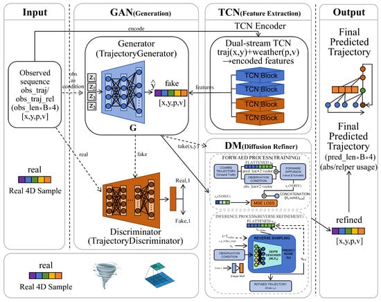
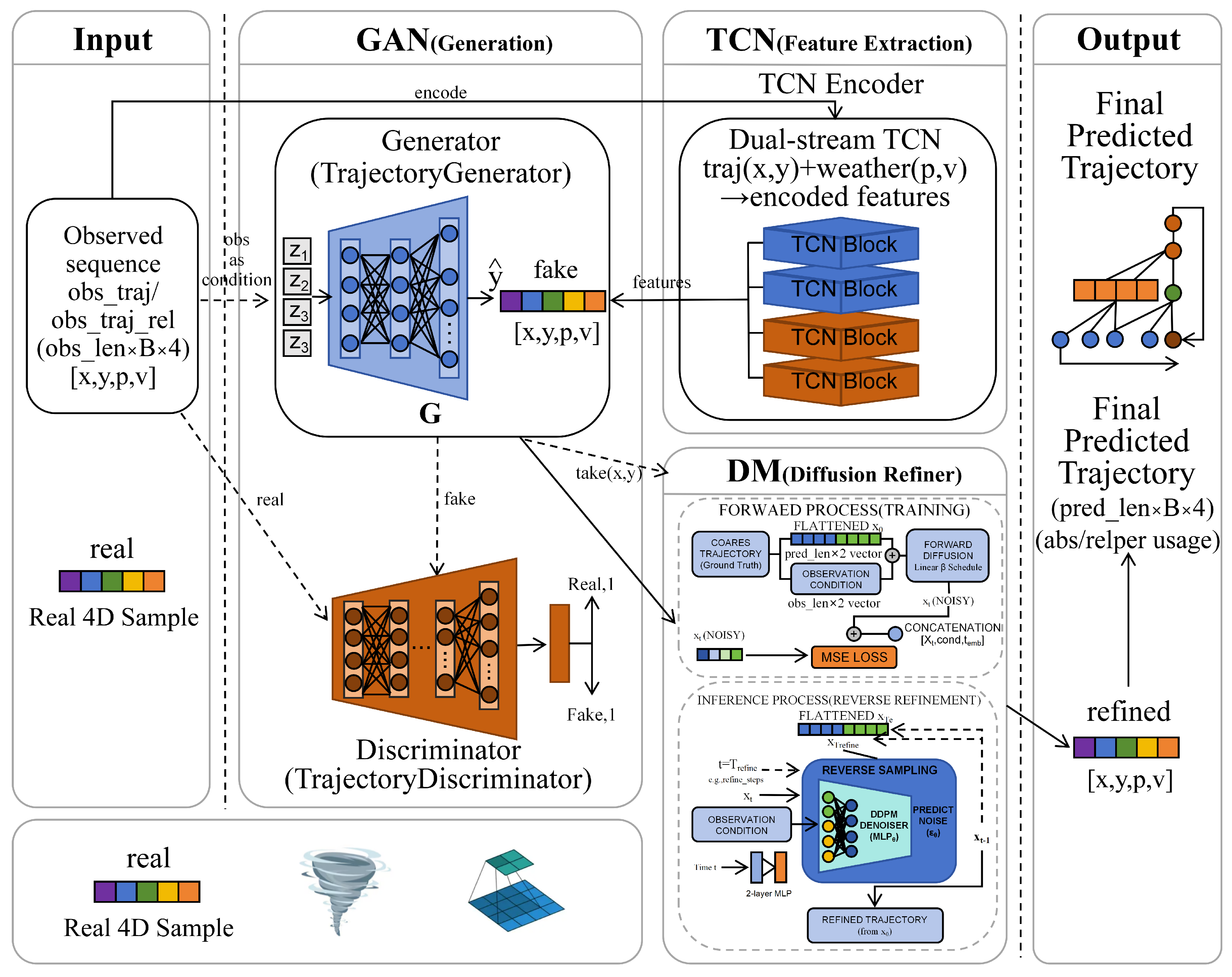
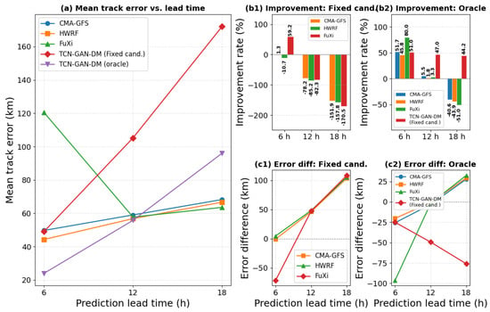
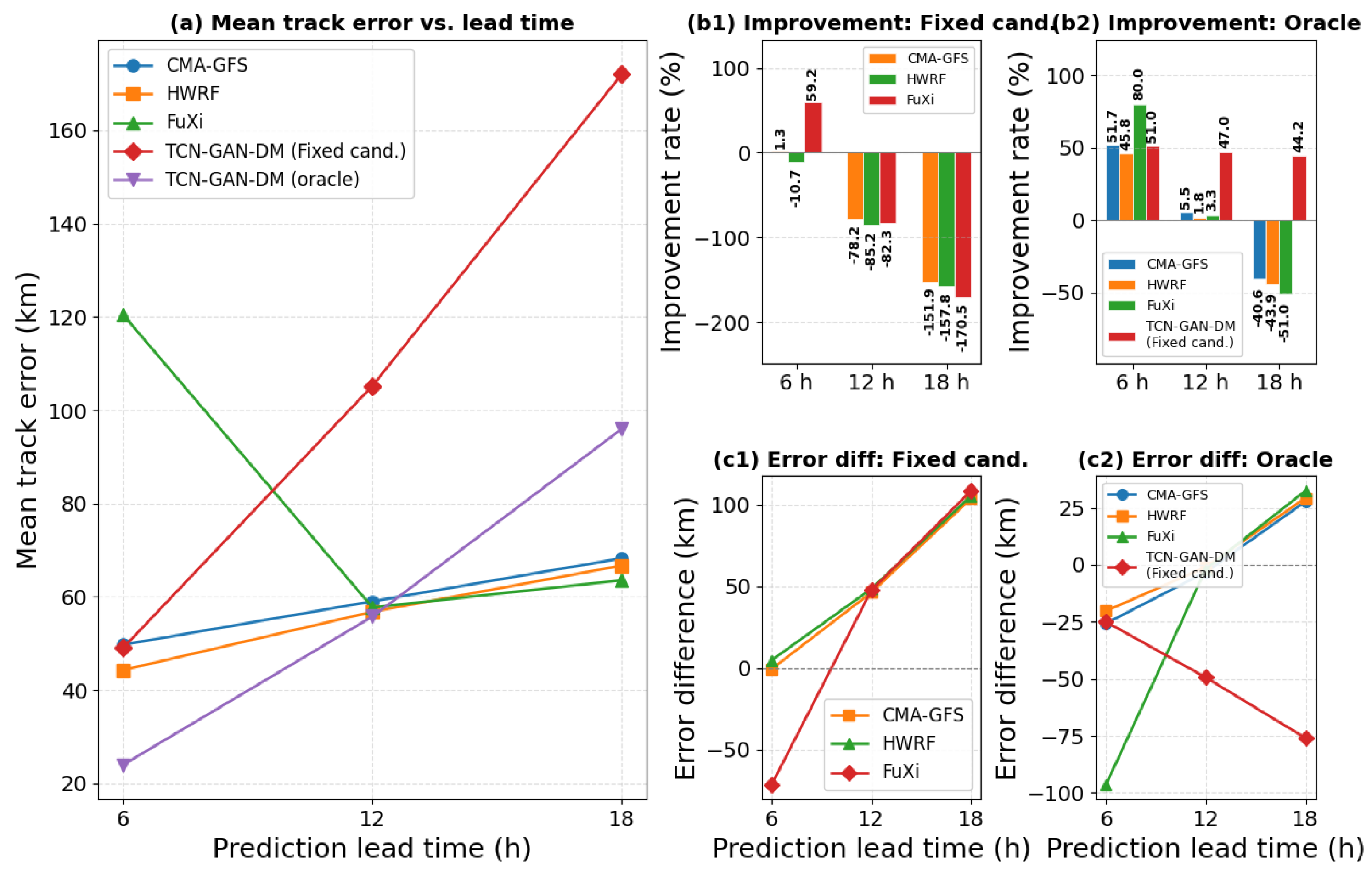
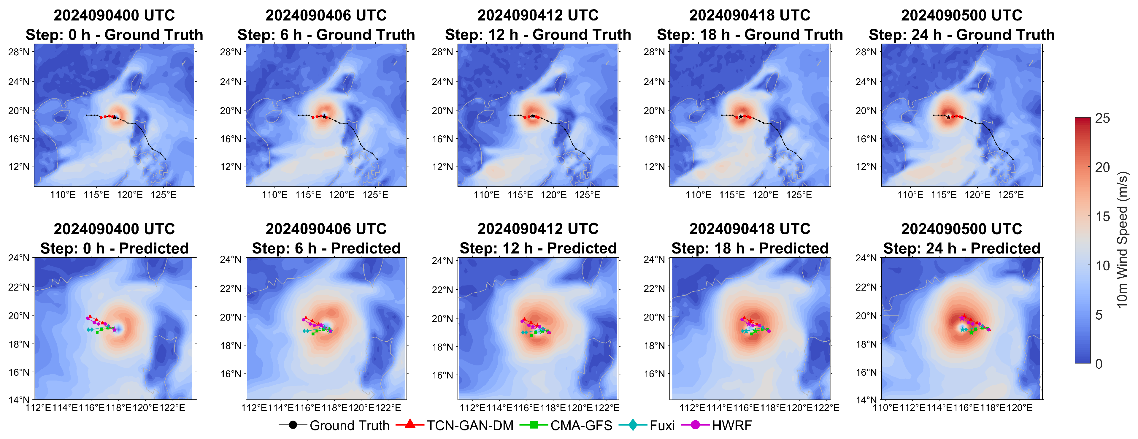
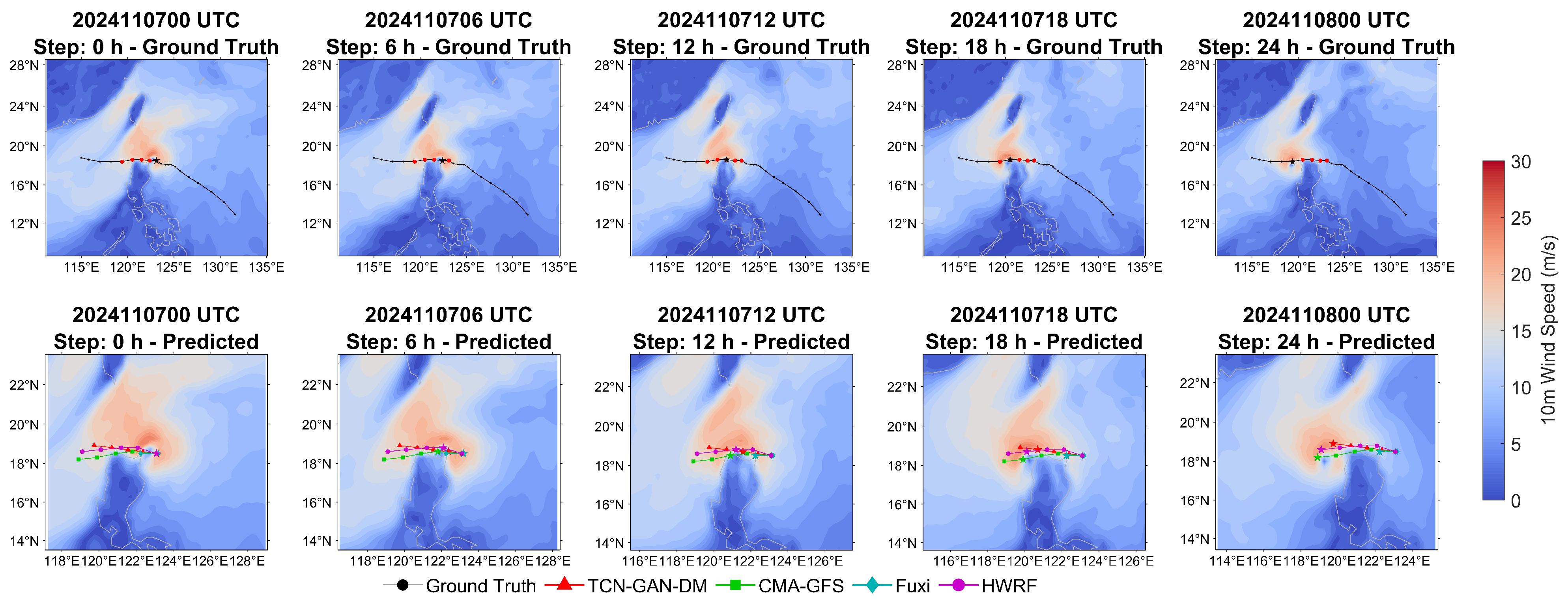
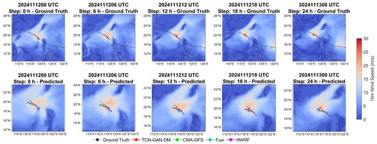
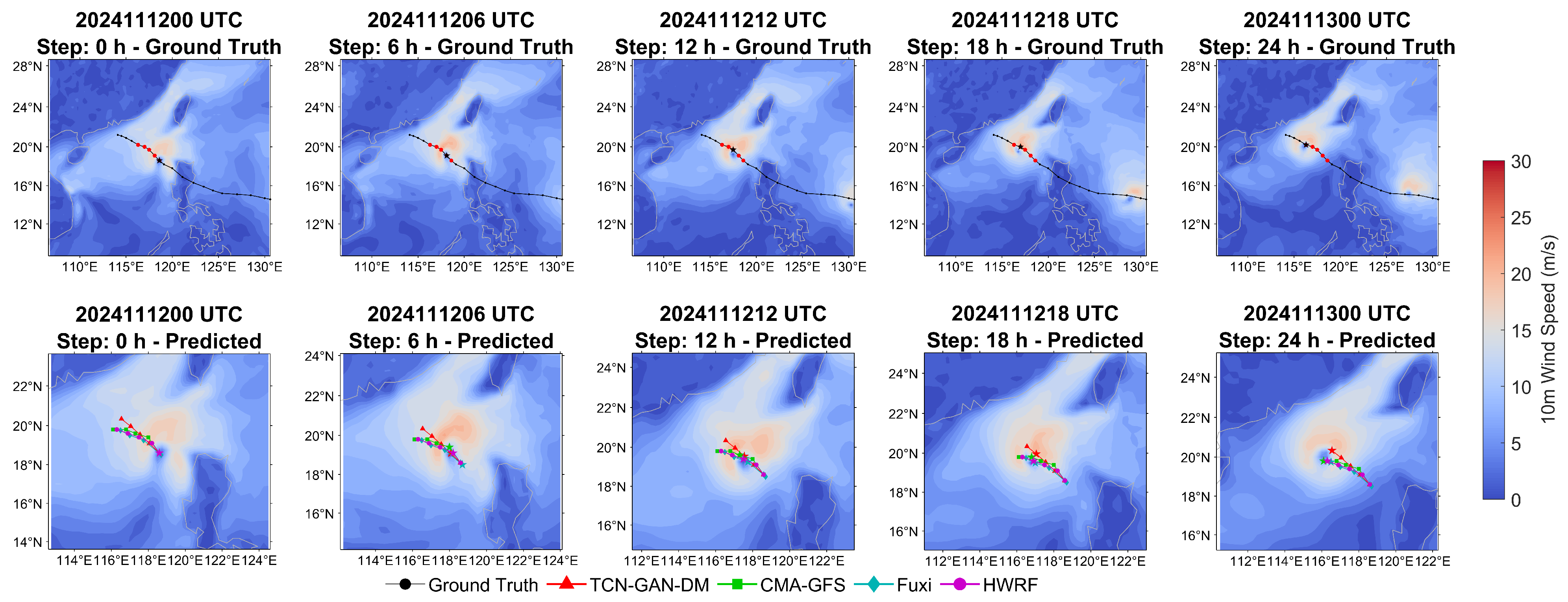
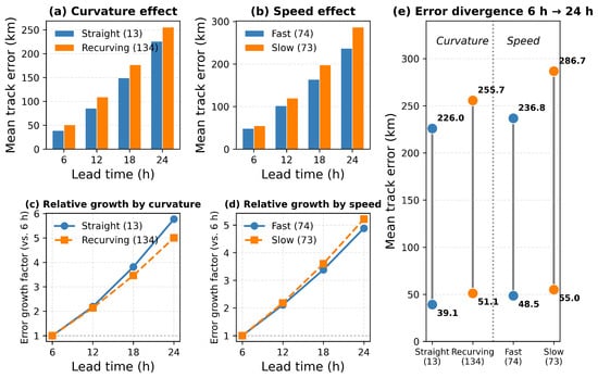
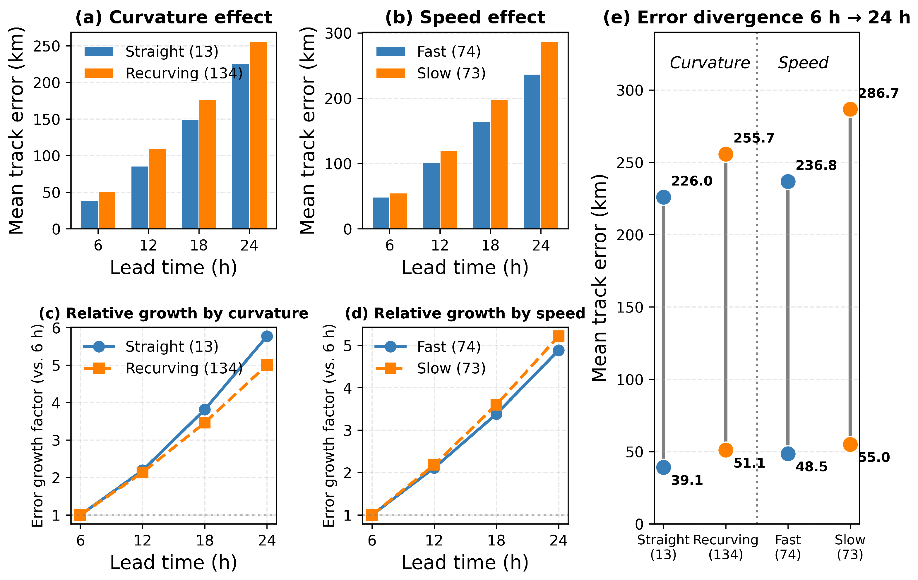
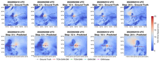
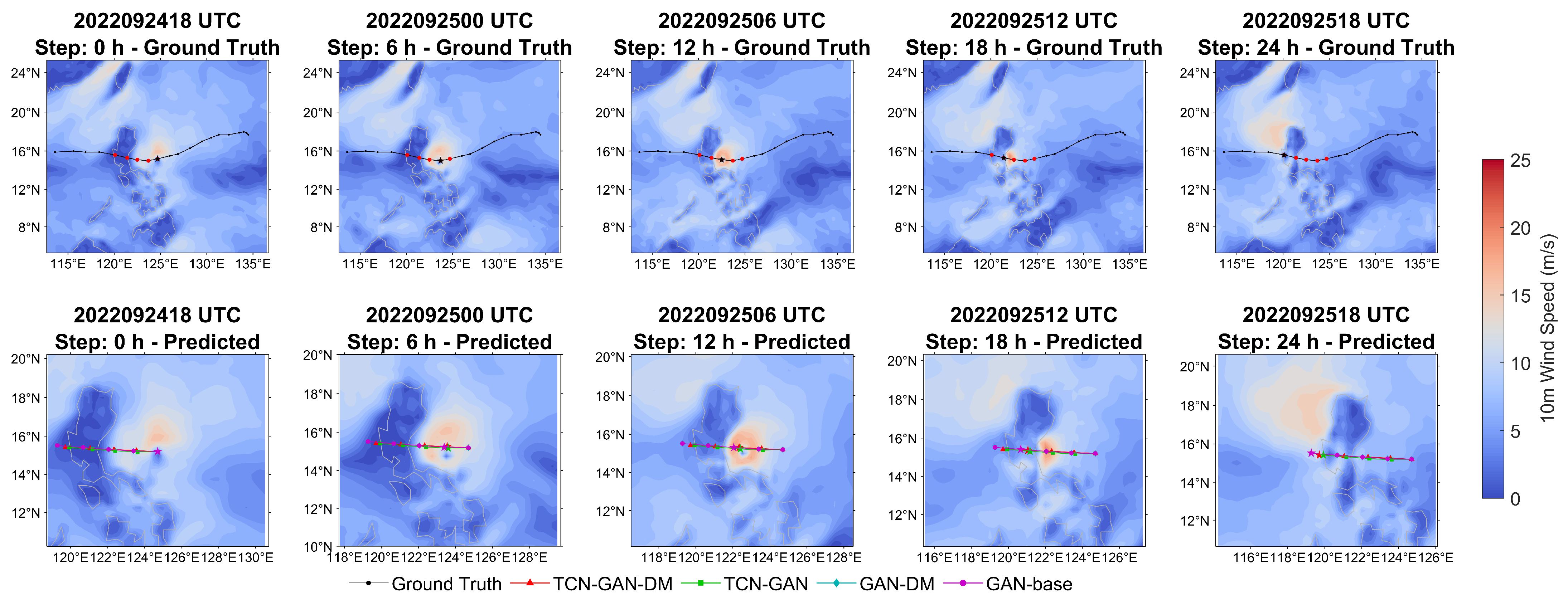
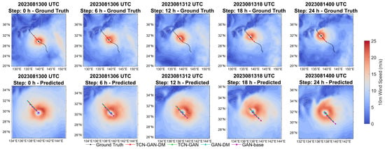
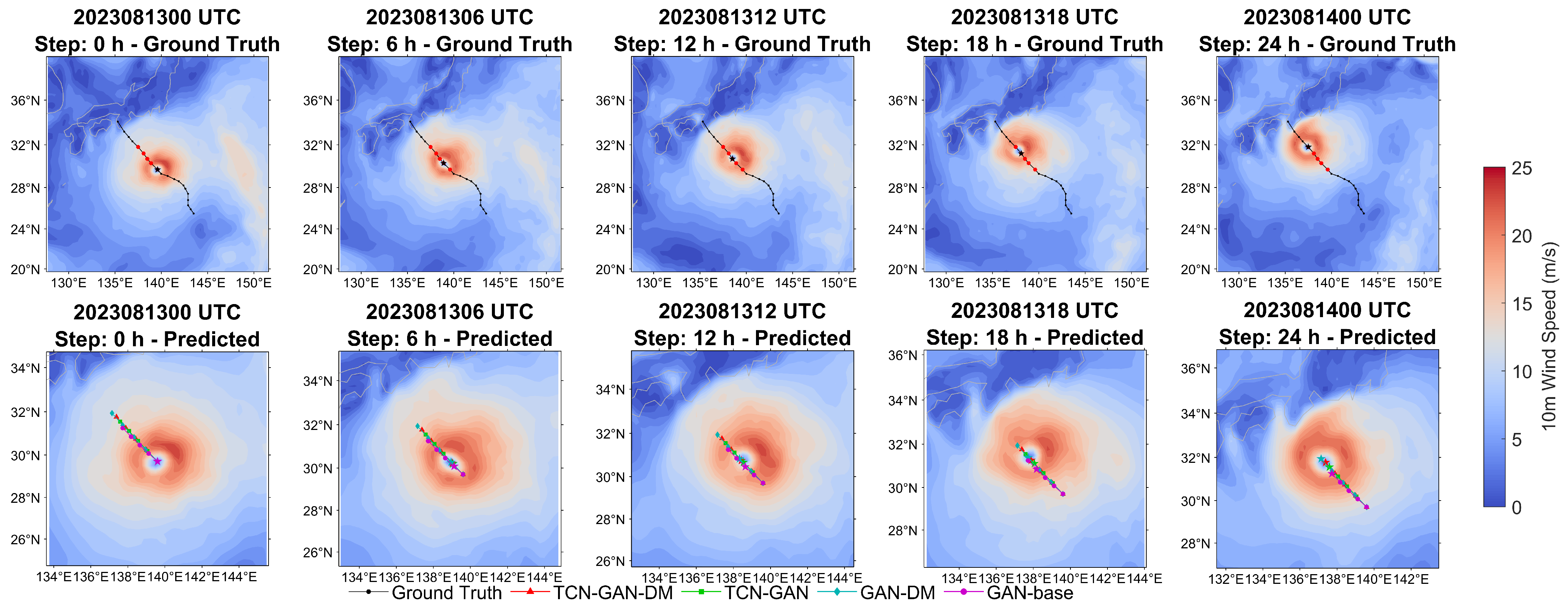

Disclaimer/Publisher’s Note: The statements, opinions and data contained in all publications are solely those of the individual author(s) and contributor(s) and not of MDPI and/or the editor(s). MDPI and/or the editor(s) disclaim responsibility for any injury to people or property resulting from any ideas, methods, instructions or products referred to in the content. |
© 2026 by the authors. Licensee MDPI, Basel, Switzerland. This article is an open access article distributed under the terms and conditions of the Creative Commons Attribution (CC BY) license.