


Abstract
In this study, we employ seven well-established machine learning algorithms for the stochastic simulation of tropical cyclones in the Northwest Pacific, namely Support Vector Machine (SVM), Random Forest (RF), Bayesian Network (BN), Backpropagation Neural Network (BPNN), Wavelet Neural Network (WNN), Recurrent Neural Network (RNN), and Long Short-Term Memory (LSTM) network. First, based on the CMA (China Meteorological Administration) Tropical Cyclone Best-Track Dataset, we statistically analyze key typhoon parameters within each 5° × 5° grid over the Northwest Pacific. Second, the Random Forest method is applied to rank the importance of feature factors for predicting typhoon translation speed, storm heading, and central pressure in each grid. Third, each algorithm is used to develop prediction models, with hyperparameters optimized via a time-series cross-validation scheme. Fourth, the prediction models are compared to identify the best-performing model for predicting translation speed, storm heading, and central pressure, respectively. The optimal models are then evaluated in terms of computational efficiency and overfitting/underfitting, and validated both against traditional statistical methods and through multi-lead-time (1–72 h) predictions for four independent typhoons: Lekima 2019, Doksuri 2023, Ragasa 2025, and Yagi 2024. The results show that the optimal machine learning models outperform traditional statistical benchmarks, achieve a direct position error of <7 km and R2 ≥ 0.979 at 1 h lead time, with track prediction remaining useful up to 48–72 h, while effective intensity prediction does not exceed 24 h. This study provides a robust data-driven framework for short-term typhoon forecasting within stochastic simulation, with future work aiming to extend to long-term predictions.
1. Introduction
Typhoon is a strong, disastrous weather event, which is often accompanied by hazards like strong winds, heavy rainfall, and huge storm surges. The densely populated and economically developed coastal cities in southeast China have suffered severe damage from typhoons, which have caused significant economic losses and human fatalities [1]. For example, Super Typhoon Lekima, making landfall in Zhejiang Province in 2019, affected the population of 14.024 million and caused direct economic losses amounting to RMB 51.53 billion [2]. The Typhoon Doksuri in 2023 affected 2.6669 million people in Fujian Province, causing direct economic loss of RMB 14.755 billion [3]. Accordingly, it is practically relevant to forecast typhoon tracks and intensities accurately for formulating rational policies on storm prevention and mitigation, as well as the reduction in casualties and property losses.
Accurate estimation of typhoon track and intensity is fundamental for forecasting and early warning. Traditionally, typhoon observation relied on sparse reports from ships and buoys, resulting in significant spatial and temporal gaps. The emergence and development of satellite remote sensing technology have fundamentally transformed this situation by enabling continuous, large-scale, and high-precision global three-dimensional observation of typhoons [4]. For typhoon positioning and track monitoring, meteorological satellites utilize high spatiotemporal resolution imagery from visible, infrared, and water vapor channels. This capability allows for clear identification of the typhoon’s eye and spiral cloud band features, thereby enabling precise calculation of the storm’s center location, movement speed, and direction—i.e., its track. Key platforms performing this task include geostationary meteorological satellites such as the U.S. GOES series [5] and Japan’s Himawari series [6], as well as polar-orbiting satellites like China’s FY-3 series [7]. In the estimation of typhoon intensity, remote sensing technology also plays an indispensable role. The Dvorak technique is the most renowned and widely applied method for this purpose [8]. It primarily relies on infrared and visible satellite cloud imagery, objectively estimating key parameters such as the maximum sustained wind speed and minimum central pressure by analyzing the structural characteristics of the typhoon’s cloud system. In summary, satellite remote sensing serves as the core means for acquiring information on typhoon track and intensity. The accurate and continuous typhoon data provided by remote sensing technology form the essential data foundation for conducting subsequent typhoon forecasting and early warning operations.
A range of methodologies currently exists for forecasting typhoon tracks and intensity. Traditional approaches are broadly categorized as either empirical or objective. Empirical methods typically integrate meteorological factors with historically analogous weather conditions to make predictions [9]. However, these methods are heavily reliant on the forecaster’s subjective experience and are consequently labor-intensive and inefficient. To address these limitations, objective methods have been developed that establish mathematical relationships between historical typhoon tracks or intensity data and the influencing climatic factors. These objective techniques primarily include dynamical [10,11,12], statistical [13,14,15,16], and statistical–dynamical models [17,18,19]. While these traditional methods perform adequately for typhoons with typical movement patterns, their effectiveness diminishes for typhoons exhibiting significant movement variations. This limitation lies in their inability to adequately capture the nonlinear features within the predictive factors.
In recent years, the rapid advancement in computer technology has led to the extensive application of artificial neural networks (ANNs) across various fields, where they have demonstrated pronounced advantages in tasks such as prediction, clustering, function approximation, and optimization [20]. This progress has introduced new perspectives for research on typhoon track and intensity forecasting. Compared to traditional prediction methods, machine learning algorithms exhibit superior capabilities in data learning, self-adaptation, generalization, and nonlinear mapping. These strengths address the limitations of conventional approaches, thereby holding significant potential for enhancing the accuracy of typhoon predictions. Nowadays, a growing body of research has been dedicated to exploring neural network-based machine learning methods for prediction, with ANNs now being actively employed in forecasting typhoon tracks and intensity [21,22,23,24,25,26,27,28,29,30,31,32]. For instance, Wang et al. [33] utilized a Backpropagation Neural Network (BPNN) model with 20 years of historical tropical cyclone track data to predict tropical cyclone trajectories. Their empirical validation against observed data confirmed the model’s considerable accuracy. Similarly, Gao et al. [34] developed a Long Short-Term Memory (LSTM) neural network model using typhoon data from 1949 to 2011, demonstrating its capability for real-time typhoon track forecasting at lead times of 6 to 24 h. In a study on typhoon intensity, Haghroosta and Ismail [35] applied both a simple ANN and an Adaptive Neuro-Fuzzy Inference System (ANFIS) optimized with genetic algorithms to data from the South China Sea (1985–2008), concluding that the ANFIS model delivered superior performance. Furthermore, Pan et al. [36] constructed a Recurrent Neural Network (RNN) model for predicting typhoon intensity based on historical data from the Northwest Pacific. Their prediction results demonstrated that the RNN model exceeded the performance of a comparative dynamical model.
This paper establishes models for forecasting typhoon tracks and intensities, employing the Empirical Track Model [37] as the foundation for typhoon stochastic simulation. Typhoon stochastic simulation is a methodology that synthesizes numerous virtual typhoons consistent with historical statistical characteristics, thereby mitigating the limitations in sample quality and quantity inherent in conventional typhoon risk analysis, which often lead to inaccurate risk assessments. The Empirical Track Model is a widely used technique in this domain [38,39], which applies statistical regression to analyze changes in typhoon translation speed, storm heading, and intensity between consecutive time steps, thereby projecting the evolution of virtual typhoon paths and strengths. To leverage the capabilities of machine learning for developing high-accuracy prediction models, seven widely recognized machine learning algorithms—Support Vector Machine (SVM), Random Forest (RF), Bayesian Network (BN), Backpropagation Neural Network (BPNN), Wavelet Neural Network (WNN), Recurrent Neural Network (RNN), and Long Short-Term Memory (LSTM)—are employed to forecast typhoon tracks and intensities using historical typhoon data from the Northwest Pacific. The optimal prediction model identified from these algorithms is subsequently applied to simulate typhoon tracks and intensities. The present work can be regarded as an enhancement of the Empirical Track Model, wherein the conventional statistical regression component is replaced with a machine learning-based predictor. This substitution is motivated by the superior ability of machine learning models to capture nonlinear relationships among variables. Thus, this study aims to identify a more effective set of machine learning algorithms for constructing prediction models for typhoon tracks and intensities within the Empirical Track Model framework, with the ultimate goal of improving the accuracy of typhoon stochastic simulation. This study provides the first comprehensive benchmark of seven machine learning algorithms within the Empirical Track Model framework, identifying the optimal model for each typhoon parameter and offering a ready-to-use stochastic simulation scheme.
The remainder of this paper is organized as follows: Section 2 delineates the core methodologies employed in the study, including the Empirical Track Model and seven widely used machine learning algorithms. Section 3 describes the data sources and preprocessing procedures utilized in the analysis. Section 4 elaborates on the development process of the prediction models. In Section 5, the optimal machine learning algorithm is identified, and the experimental results are analyzed. Finally, Section 6 concludes the paper with a summary of the study.
2. Technology
2.1. Empirical Track Model
Based on the HURDAT (Hurricane Best-Track Database) dataset [40], an Empirical Track Model, a popular employed approach in typhoon stochastic simulation, was established. It describes the regression relationship between typhoon translation speeds, storm headings and relative intensities at the next moment i + 1 and the current moment i, as shown in Equations (1)–(3).
where ci represents typhoon translation speed at time step i; θi represents storm heading at time step i; Ii represents the relative intensity which was proposed by Darling [41]; a, b, and d are the linear regression coefficients; ψ and λ are the latitude and longitude of typhoon center; Δlnc = lnci+1 − lnci and Δθ = θi+1 − θi; the time interval between adjacent moments is 6 h; is the monthly mean Sea Surface Temperature (SST); and εc, εθ, and εI are random error terms with zero mean.
The Atlantic Basin was initially partitioned into 5° × 5° grids (by latitude and longitude) by Vickery et al. [37], who systematically compiled historical hurricane translation speeds, storm headings, and intensities within each grid. Through regression analysis, the parameters ai, bi and di were determined for every grid cell. Subsequently, they employed a direct sampling method to extract initial typhoon information—including starting location, genesis date, heading, translation speed, and intensity—from the HURDAT dataset, which was used to initialize the simulation program. Based on a given initial typhoon state, the translation speed, heading, and intensity were computed using Equations (1)–(3), enabling the estimation of the typhoon’s position and intensity at subsequent 6 h intervals. By iterating this process, a complete synthetic typhoon track was generated.
2.2. Machine Learning
2.2.1. Support Vector Machine
Support Vector Machine (SVM) is a machine learning technique developed on the basis of statistical learning theory and Vapnik–Chervonenkis theory, following the principle of structural risk minimization [42]. It has a high capacity for generalization and adaptability. As illustrated in Figure 1, the support vectors are the data points located on the classification boundary. SVM maps the input space to a higher-dimensional feature space through a nonlinear transformation. In the high-dimensional space, a hyper-plane is sought that both minimizes classification errors and maximizes the margin between the hyper-plane and the nearest data points (i.e., the support vectors) [43,44].
Figure 1.
The framework of SVM.
Support Vector Regression (SVR) is a machine learning method for regression analysis via SVM. To reduce model complexity and enhance prediction performance, the SVR model employs a kernel function to map the data into a high-dimensional space, facilitating the identification of the optimal regression hyper-plane. The kernel function effectively addresses the dimensionality problem and overcomes the problems of slow convergence, local minima, overfitting, and underfitting in machine learning methods.
Assuming that the training dataset is , is the number of samples. The input feature space is first mapped to the high-dimensional feature space , as shown in Equation (4), and then the regression analysis is performed [45,46].
where is the high-dimensional feature space. represents the weight coefficient, and denotes the bias coefficient. According to the modeling of the error and the parameterized objective function, SVR can be classified into two categories, namely ε-SVR and ν-SVR. For ε-SVR, the optimization problem is shown in Equation (5).
The constraint is as follows:
In Equation (6), are the slack variables. is the insensitivity coefficient, which controls the width of the area in which the regression function is insensitive to the data samples [47]. is the penalty parameter, which controls the degree of penalization for samples that exceed . In general, a larger value of leads to a better fit to the data, but a poorer generalization ability [48].
For ν-SVR, the optimization problem is shown in Equation (7).
The constraint is expressed by the following equations:
Solving the above optimization problem to obtain the SVR model, shown in Equation (9).
where are Lagrange multipliers. is the kernel function, which serves to reduce the computational complexity by avoiding computation on the high-dimensional feature space . The basic kernel functions are the linear kernel function , the polynomial kernel function , the radial basis function , and the sigmoid kernel function . , and are kernel function parameters [49].
2.2.2. Random Forest
Random Forest (RF), an ensemble learning algorithm proposed by Breiman, is widely used for classification, regression, and feature selection [50]. It improves model generalization by combining multiple decision trees. The core idea of RF is to achieve robust predictions based on Bootstrap aggregation (Bagging) and stochastic feature selection, thereby reducing the variance and correlation of individual decision trees. The structure of the RF regression algorithm is shown in Figure 2. First, m samples are randomly drawn from the original training set with replacement using Bootstrap sampling, allowing duplicates, to generate multiple sub-training sets. Then, a decision tree is trained independently for each sub-training set based on the classification and regression tree (CART) algorithm. Finally, the result is obtained by taking the average of all the decision tree outputs.
Figure 2.
Regression calculation process of RF.
CART is an algorithm for recursively constructing binary trees, which recursively divides the current set of samples into two subsets at each node except the leaf nodes until a stopping condition is satisfied. Assuming that is a subset of samples, and are the input samples and output variables, respectively. The construction process of the CART algorithm is as follows:
- (1)
- Construct a root node that contains the entire sample subset.
- (2)
- Traverse all features. For feature j, the sample set is partitioned by the cutoff point . First, the values of feature j for all samples in the subset are ranked in ascending order. Then, the cutoff point is determined as the average of two adjacent values in the sorted sequence. Based on the cutoff point , the feature space of the sample subset is partitioned into two subspaces and where , , , . and represent the average values of the output variable in the subspaces and , respectively. To identify the optimal features and cutoff points for partitioning the sample set, the minimum mean squared error is calculated as in Equation (10).
- (3)
- Repeat steps (1) and (2) for the two subspaces until the entire decision tree is fully constructed and all the samples in the subset are assigned to leaf nodes [51,52,53,54,55]. The leaf nodes are shown as green circles in Figure 2.
2.2.3. Naive Bayesian
Naive Bayesian (NB) classifier is a simple probabilistic classifier based on Bayes’ theorem and the assumption of conditional independence of attributes [56]. The fundamental principle of classification is to assign a given instance to the category with the highest posterior probability based on the occurrence of that instance. We will briefly discuss details of the NB technique. For a detailed mathematical background of the NB approach, refer to [57,58]. The classification flowchart is shown in Figure 3, and the specific implementation steps are as follows:
Figure 3.
Flowchart of the NB model.
- (1)
- Let the feature vector be a term to be classified. represents a characteristic attribute of .
- (2)
- Assume a category ; its prior probability is given by Equation (11).where denotes the number of categories and indicates the total number of training samples.
- (3)
- Determine the conditional attribute , which is given by Equation (12).where represents the number of occurrences of under category , indicates the total number of .
- (4)
- Determine the posterior probability that the item to be categorized belongs to each category, i.e., , which is calculated by Equation (13).
- (5)
- If , then is considered to belong to class k.
2.2.4. Backpropagation Neural Network
Backpropagation Neural Network (BPNN) was first proposed by Werbos in 1974 and developed into the BP algorithm by Rumelhart et al. in 1985 [59]. BPNN has powerful nonlinear modeling capabilities and is widely used in classification, regression, pattern recognition, and other fields. The core principle is to optimize the network weights and minimize the prediction error by the gradient descent method.
The BP algorithm learning process consists of two processes: forward propagation of the signal and backpropagation of the error. In forward propagation, input samples are processed through the hidden layer and then transmitted to the output layer. If the actual output of the output layer does not match the desired output, then it moves to the backpropagation stage of the error. A backpropagation mechanism passes the output layer error to the input layer, accurately distributing it across all neurons. In this way, the error signals obtained for each layer of neurons will be used as an important basis for adjusting the weights of the corresponding neurons. The process of adjusting the weights through forward signal propagation and error backpropagation is iterated until the network output error is reduced to an acceptable level or a predetermined number of training iterations is reached [60].
Considering a BPNN with three layers, its architecture is presented in Figure 4. The input vector is , the hidden layer is represented as , and the output layer is denoted as . The forward propagation of the signal is as shown in Equation (14).
where denotes the connection weight from the input layer to the hidden layer, and represents the bias of the hidden layer. denotes the connection weight from the hidden layer to the output layer and represents the bias of the output layer. is the activation function. Based on the prediction output y of the network and the desired output ytarget, the prediction error of the network is calculated by Equation (15).
Figure 4.
The illustration of the BP neural network.
The weights and biases are sequentially corrected based on an error gradient descent method. The details of this method can be found in [59].
2.2.5. Wavelet Neural Network
Wavelet Neural Network (WNN) is a hybrid model that combines the advantages of wavelet analysis and artificial neural networks. It enhances the time-frequency localized characterization of nonlinear and nonsmooth signals by introducing the wavelet basis function as the hidden-layer activation function. The input signal is decomposed into sub-signals of different scales and locations by wavelet transform. Then, the neural network is used to adaptively optimize the scale factor, translation factor and network weights of the wavelet basis function to achieve multi-resolution feature extraction and dynamic modeling. The wavelet basis function introduces two new parameter variables, namely the scale factor and the translation factor. Assuming that the input signal sequence is , the output of the hidden layer is calculated by Equation (16).
where is the output of the jth node of the hidden layer and represents the wavelet basis function. and are the translation and scale factors of the wavelet basis functions, respectively. Compared with traditional neural networks, WNN exhibits significant advantages in noise suppression and local feature learning.
2.2.6. Recurrent Neural Network
A Recurrent Neural Network (RNN) is a neural network designed to process sequential data by introducing a temporal recursive structure to capture temporal dependencies. RNN establishes connections between nodes in the hidden layers, allowing the input to the hidden layer to be not only the input of the current moment but also the output of the hidden layer of the previous moment. In this way, the RNN can memorize previous information in the network [61]. As illustrated in Figure 5, the architecture of an RNN and a feed-forward neural network is roughly the same, with the primary difference being the linkage between their hidden layers. The forward propagation of the signal can be expressed as Equation (17).
where denotes the connection weight from the input layer to the hidden layer, and represents the bias of the hidden layer. denotes the connection weight from the hidden layer to the output layer and represents the bias of the output layer. , , and denote the network input, the hidden-layer output, and the network output at time t, respectively. represents the activation function.
Figure 5.
RNN architecture diagram.
2.2.7. Long Short-Term Memory Network
Long Short-Term Memory (LSTM), proposed by Hochreiter and Schmidhuber, is introduced to address the issues of gradient vanishing and gradient explosion caused by long-term dependency of RNN in the prediction process [62]. It has evolved into an effective and scalable model and has been effectively implemented across a multitude of domains. The core of LSTM is the cell state and three gating mechanisms (forget gate, input gate, and output gate). It controls the information flow through the gates [63,64]. As depicted in Figure 6, f, i, o, c, and h denote the forget gate, input gate, output gate, cell state, and output, respectively. denotes the sigmoid activation function and tanh denotes the hyperbolic tangent activation function. At time step t, the structure is shown in Figure 6.
Figure 6.
Architecture of LSTM.
- (1)
- Forget gate, shown in Equation (18):
The forget gate determines how much historical information is preserved. and denote the weight matrix and bias, respectively.
- (2)
- Input gate, shown in Equation (19):
The input gate mainly filters information to the cell state. is the information filtered by the sigmoid function that needs to be updated. is the candidate cell state.
- (3)
- Cell state, shown in Equation (20):
The cell state retains long-term characteristics through a linear accumulation mechanism.
- (4)
- Output gate, shown in Equation (21):
The output gate mainly generates the current hidden state.
3. Data Source and Preprocessing
The historical typhoon data from 1949 to 2021 used in this study were obtained from the Tropical Cyclone Best-Track Database maintained by the China Meteorological Administration (CMA; available at https://tcdata.typhoon.org.cn) [65]. This dataset was obtained primarily from satellite observations, with the support of marine station data and numerical models, and systematically documents all tropical cyclones in the Northwest Pacific and those affecting the coastal regions of China since 1949 at 6 h intervals, providing parameters such as the typhoon name, timestamp, central pressure, and geographic location (longitude and latitude). The CMA Best-Track Dataset determines typhoon position and intensity primarily by analyzing multi-source satellite remote sensing imagery.
This study employs the best-track data of historical typhoons spanning from 1949 to 2021. However, the data from 1949 to 1970 are subject to inconsistencies due to changes in anemometer technology, resulting in systematic discrepancies compared to later records. To ensure data homogeneity, we applied the correction method proposed by Li et al. [66] to the pre-1970 records. Additionally, tropical depressions and typhoons that underwent extratropical transition were excluded from the analysis, as referred to in [67].
The establishment of the prediction model for typhoon track and intensity requires its central pressure, location, translation speed, and storm heading. Translation speed and storm heading need to be calculated by the typhoon position at adjacent moments. The storm heading θ denotes the angle between the direction of translation and true north, and it is considered positive when the rotation is clockwise. The translation speed c of the typhoon center can be derived from Equation (22)
where ΔLat (ΔLon) represents the change in latitude (longitude) between successive time intervals (6 h) and β is a distance parameter related to the latitude [68].
In addition, the generation and development of typhoons are inextricably associated with Sea Surface Temperature (SST). Therefore, SST is not negligible in the construction of the typhoon intensity model. The SST data are retrieved from the Physical Sciences Laboratory of the National Oceanic and Atmospheric Administration (NOAA), and the spatial resolution is 1°. The SST data product is primarily derived from satellite remote sensing, supplemented and calibrated by in situ observations, and ultimately generated through data assimilation and fusion techniques. To enhance model performance, the input data for all the models were normalized.
4. Establishment of the Model
Following the framework of the Empirical Track Model, the Northwest Pacific region was partitioned into 5° × 5° grid cells, for which prediction models of typhoon translation speed, storm heading, and intensity were developed. To define the input samples for these models, potential features were selected based on Reference [37], as summarized in Table 1. Historical tracks were categorized into easterly headed and westerly headed storms to better capture movement characteristics before and after recurvature. Consequently, separate prediction models for translation speed and direction were constructed for each type. Furthermore, key parameters required for the track and intensity prediction models—including translation speed, heading, and central pressure—were computed from the historical typhoon data (1949–2021) within each grid cell. This process facilitated the construction of the requisite sample dataset. Finally, the sample sizes for building the prediction models were calculated separately for each grid cell, as illustrated in Figure 7.
Table 1.
Potential features for typhoon translation speed, storm heading, and intensity prediction models.
Figure 7.
The sample size in each grid from westerly and easterly (in brackets) headed storms derived from historical observations. The color indicates the total number of samples within each grid cell.
For each grid cell, the temporally ordered typhoon tracks were split chronologically, with the first 80% of events used for training and the remaining 20% for validation. Additionally, any grid cell with fewer than 50 samples was assigned the prediction model from an adjacent, data-sufficient cell.
In Table 1, typhoon features involved in the translation speed prediction model include the translation speed at the previous three moments ci−2, ci−1 and ci; the storm heading at the previous two moments θi−1 and θi; the longitude ψ and latitude λ of the typhoon center. The output data is the translation speed at the next moment, ci+1. Typhoon features involved in the storm heading prediction model include the storm heading at the previous three moments θi−2, θi−1 and θi; the translation speed at the previous two moments ci−1 and ci; the longitude ψ and latitude λ of the typhoon center. The output data is the storm heading at the next moment, θi+1. Features involved in the typhoon intensity model are the central pressure at the previous three moments pi−2, pi−1 and pi, the monthly mean sea surface temperature and . The output data is the central pressure at the next moment pi+1.
Given the multitude of potential predictors in Table 1, using all the factors for model training can lead to increased complexity and overfitting. This necessitates careful feature selection to identify and retain the most relevant and influential typhoon characteristics for model development. Utilizing Random Forest (RF) for feature importance ranking represents a classical machine learning methodology for feature selection. The RF algorithm quantifies prediction error for individual decision trees using Out-of-Bag (OOB) samples, thereby assessing tree accuracy. Subsequently, values of a specific feature are randomly permuted within the OOB samples, and the corresponding perturbed error is recalculated. The importance score for each feature is derived from the mean error increase across all the trees. A more substantial increase in error following permutation indicates a greater contribution of that feature to the model’s predictive capability.
Figure 8a and Figure 8c respectively show the features’ order of importance in the translation speed model for easterly and westerly headed storms, calculated using the RF method. To forecast the typhoon translation speed over the subsequent 6 h period, the speed recorded at the preceding timestep proves critical. However, the potential contribution of incorporating less-predictive features warrants further investigation. The OOB scores under different input feature dimensions are computed, with variables input in the order of importance, as shown in Figure 8b,d. Analysis of Figure 8b reveals that for the easterly translation speed model, the OOB score attains a local maximum when incorporating the top four features ranked by importance. Subsequent introduction of additional features yields diminishing improvements in the OOB score, thus identifying the initial four-feature subset, i.e., ci, ψ, λ and θi, as the optimal input combination. Similarly, for the westerly translation speed model (Figure 8d), optimal predictive performance is achieved whereby the top five most significant features (ci, λ, ψ, ci−2 and θi−1) constitute the model input.
Figure 8.
The importance index of features in the translation speed prediction model for easterly (a) and westerly (c) headed storms and the OOB_score (b,d) of different feature combinations based on the RF (red dot indicates the optimal feature subset).
For translation speed, the dominant role of ci reflects the strong inertia of a tropical cyclone’s movement. In the atmosphere, the vortex’s momentum resists rapid changes in propagation speed, consistent with the near-persistence observed in best-track data. The secondary importance of latitude (ψ) and longitude (λ) captures the β-effect, the poleward and westward drift induced by the latitudinal gradient of the Coriolis parameter.
Figure 9 shows the features’ order of importance in the storm heading model for easterly and westerly headed storms, calculated using the RF method. For easterly headed typhoons, the OOB score peaks when incorporating the top six features, whereas for westerly headed typhoons, it attains a local maximum using the top five features. Therefore, θi, θi−1, θi−2, ψ, λ and ci−1 constitute the optimal input for the easterly storm heading model, and θi, θi−1, θi−2, λ and ψ constitute the optimal input for the westerly storm heading model.
Figure 9.
The importance index of features in the storm heading model for easterly (a) and westerly (c) headed storms and the OOB_score (b,d) of different feature combinations based on the RF (red dot indicates the optimal feature subset).
For storm heading, the high importance of θi and θi−1 reflects the persistent nature of steering flow. In the western North Pacific, the subtropical high and monsoon trough provide a slowly varying large-scale environment, so changes in heading are typically small between consecutive 6 h steps. The inclusion of longitude and latitude again relates to the spatial variability of the steering current. For example, as a typhoon moves northward, it encounters the westerlies and may recurve.
Figure 10 shows the features’ order of importance in the typhoon intensity model, calculated using the RF method. The OOB score peaks when incorporating the top two features. Therefore, pi and pi−2 constitute the optimal input for the typhoon intensity model.
Figure 10.
(a) The importance index of features in the typhoon intensity model and (b) the OOB_score of different feature combinations based on the RF (red dot indicates the maximum value).
For central pressure (intensity), the overwhelming importance of pi and pi−2 indicates that intensity evolution is dominated by autocorrelation, i.e., the storm’s own thermodynamic structure. The weaker role of SST may be explained by the fact that SST affects intensification primarily through ocean heat content and air–sea fluxes, which are not directly represented by the monthly mean SST used here; a higher-resolution, time-varying SST product might improve the physical link.
5. Results
To assess the prediction models effectively and search for the optimal prediction models for translation speeds, storm headings and central pressures of typhoons, the adjusted coefficient of determination (R2) and Root Mean Square Error (RMSE) between the predicted and observed results in the testing set are calculated by Equations (23) and (24)
where represents the observed values, indicates the average value of . denotes the value obtained through forecasting, n represents the sample size, and k indicates the number of predictor variables. Adjusted R2 (hereinafter referred to as R2) can mitigate the overfitting problem caused by an excessive number of independent variables, providing a more objective evaluation of the model’s explanatory power. Its value typically ranges from 0 to 1, with a higher value indicating a better model. RMSE is a widely used metric to quantify the deviation between a model’s predicted values and the true values. A smaller RMSE indicates higher prediction accuracy of the model.
Identifying the optimal prediction model for typhoon track and intensity entails two key tasks: internal hyperparameter tuning and comparative selection among different modeling architectures. Seven machine learning algorithms—SVR, RF, NB, BPNN, WNN, RNN, and LSTM—were selected to construct prediction models for typhoon track and intensity based on remote sensing-derived best-track data. For each algorithm, we first undertook an internal hyperparameter optimization using a grid search to identify the configuration that yielded the best performance. Subsequently, we conducted a comparative performance evaluation among these seven optimized algorithms to determine the overall optimal model for the prediction tasks. Finally, based on the established optimal model, we simulated and compared the actual typhoon tracks and intensities (Lekima, 2019 and Doksuri, 2023) and compared them with the prediction results of statistical models for validating the accuracy of the established optimal model.
5.1. Model Internal Optimization
To ensure fair and robust hyperparameter selection for each mode, a time-series-aware cross-validation procedure was implemented. For each grid cell, the temporally ordered training set (the first 80% of samples) was split into four consecutive blocks. For a given hyperparameter combination, three validation cycles were performed:
- Fold 1: train on Block 1, validate on Block 2;
- Fold 2: train on Blocks 1–2, validate on Block 3;
- Fold 3: train on Blocks 1–3, validate on Block 4.
The average performance (e.g., RMSE and R2) across the three validation blocks was taken as the score for that hyperparameter combination. The combination with the best average score was finally selected for the model.
5.1.1. SVM
SVM is applicable to both classification and regression tasks; in this study, we employed it for regression. The SVM regression framework primarily comprises two algorithms: ε-SVR, which utilizes the epsilon parameter to define an error-insensitive interval, thereby enhancing robustness to noise, and ν-SVR, which controls the number of support vectors via the parameter ν, as detailed in Section 2.2.1. Four kernel functions are commonly used in SVR modeling: linear, polynomial, radial basis function, and sigmoid. To identify the optimal hyperparameter configuration for the SVR model, we designed eight distinct experimental groups, as outlined in Table 2. The combinations of ε-SVR with the four kernel functions are designated SVR_S1 through SVR_S4, while the combinations of ν-SVR with the kernels are designated SVR_S5 through SVR_S8.
Table 2.
Experimental configurations for the SVR model.
We conducted eight experiments of SVR in Table 2 for typhoon track and intensity models. Taking the translation speed model of westerly headed storms as an example, Figure 11 presents heatmaps of the R2 and RMSE for the SVR_S1 and SVR_S2 model predictions within each grid cell across the Northwest Pacific. It should be noted that blank grids in Figure 11 indicate either insufficient sample sizes within those grids or poor model prediction performance; thus, no corresponding predictive model was established. As shown in Figure 11a,b, the R2 for typhoon translation speed predictions by the SVR_S1 model ranges between 0.5 and 1 in the vast majority of grid cells, while the RMSE remains below 5. These results demonstrate the relatively strong predictive performance of the model. However, in Figure 11c, the R2 for the vast majority of grids is around 0.5, while in Figure 11d, the RMSE exceeds 5, indicating that the SVR_S2 model performs poorly. The comparison of prediction results between the SVR_S1 and SVR_S2 models clearly highlights the necessity of model hyperparameter tuning in this study.
Figure 11.
Adjusted R2 and RMSE of the test set results for typhoon westerly translation speed predicted by the SVR_S1 model (a,b) and SVR_S2 model (c,d) across grid cells in the Northwest Pacific.
To evaluate the model performance across all grid cells in the Northwest Pacific, we used the mean R2 and mean RMSE of all the grid cells in the test set as an indicator. For translation speed from easterly and westerly headed storms, we calculated the average R2 and RMSE across all the grid cells in models SVR_S1 through SVR_S8 respectively. It is clear from Figure 12 that the R2 of the four experiments, SVR_S2, SVR_S4, SVR_S6, and SVR_S8, are relatively low, and the RMSEs are relatively high for both easterly and westerly headed storms. It indicates that the polynomial kernel function and the sigmoid kernel function perform relatively poorly. The performance of the other four experiments was not significantly different, but SVR_S1 and SVR_S5 performed slightly better overall. Comparing the mean R2 between SVR_S1 and SVR_S5 (or SVR_S2 and SVR_S6 or SVR_S3 and SVR_S7 or SVR_S4 and SVR_S8), it can be found that the results are not significantly different, indicating that the two algorithms of ε-SVR and ν_SVR have little impact on the prediction results. Furthermore, Figure 12 reveals that while the R2 for eastward and westward translation speeds is comparable, the RMSE of westerly headed typhoons is substantially lower than that of their easterly headed counterparts. This discrepancy is primarily attributed to the significantly larger sample size of westward-moving typhoons, which enhances model generalization capability.
Figure 12.
Comparison of the mean adjusted R2 (a) and RMSE (b) across eight parametric configurations of the SVR prediction model for translation speed from easterly and westerly headed storms.
Table 3 presents the performance (R2) of the models for predicting typhoon translation speed, storm heading, and central pressure under eight experimental setups (SVR_S1 to SVR_S8). The analysis reveals consistent patterns between storm headings and central pressures with typhoon translation speeds. Consequently, the hyperparameters from either SVR_S1 or SVR_S5, i.e., ε-SVR or ν-SVR and linear kernel function, are selected as optimal configurations for the SVR model to simultaneously predict the typhoon translation speeds, storm headings, and central pressures, whether for easterly or westerly headed storms.
Table 3.
R2 performance of SVR models with different configurations for predicting typhoon translation speed (C), storm heading (θ) in east and west directional components, and central pressure (P). The boldfaced values in the table indicate the best model performance.
5.1.2. RF
We conducted experiments on three pivotal hyperparameters in the RF model: the number of decision trees, the maximum number of splits per individual tree, and the minimum sample size of leaf nodes. These parameters collectively determine the model’s predictive performance. The tree count determines the ensemble size, where increasing trees enhances prediction robustness at the expense of computational overhead. The maximum split depth, defined as the longest root-to-leaf path length in a decision tree, critically regulates model complexity: shallow depth induces underfitting; excessive depth causes overfitting. The minimum leaf samples specify the least observations required in terminal nodes; higher values enhance noise robustness at the cost of reduced pattern granularity. In this paper, the number of decision trees was given as 100 and 300, the maximum number of splits per individual tree was given as 10 and 30, and the minimum sample sizes of leaf nodes were given as 2, 5 and 9. The experimental configurations for hyperparameter combinations are detailed in Table 4.
Table 4.
Experimental configurations for the RF model.
Figure 13 presents the mean R2 and RMSE values across twelve RF experiments (RF_S1 to RF_S12) for predicting the storm heading of both easterly and westerly headed storms. It demonstrates minimal variation in both R2 and RMSE metrics across distinct RF configurations (RF_S1–RF_S12), indicating the storm heading prediction model exhibits low sensitivity to hyperparameter adjustments within the tested range. This robustness may originate from the proximity of all the configurations to near-optimal parameter settings. Nevertheless, RF_S10 consistently yielded optimal performance metrics in storm heading prediction for both easterly and westerly headed storms, achieving peak R2 values and near-minimal RMSE. Analogous performance trends were observed in the RF models forecasting typhoon translation speed and central pressure, as shown in Table 5. The performance of each model under different experimental setups is presented. We therefore designate RF_S10’s hyperparameter configuration, specifically number of decision trees = 300, maximum number of splits = 30, and minimum number of samples in leaf nodes = 2, as the optimal parameter set for typhoon track and intensity forecasting models employing RF methodology.
Figure 13.
Comparison of the mean adjusted R2 (a) and RMSE (b) across twelve experimental configurations in the RF prediction model for storm heading from easterly and westerly headed storms.
Table 5.
R2 and RMSE performance of RF models with different configurations for predicting typhoon translation speed (C), storm heading (θ) in east and west directional components, and central pressure (P). The boldfaced values in the table indicate the best model performance.
5.1.3. NB
Kernel Density Estimation can be extended to regression problems within Naïve Bayes frameworks. There are four commonly used kernel functions in Naive Bayesian: the normal kernel function, box kernel function, triangle kernel function, and Epanechnikov kernel function. We designed four experimental configurations—NB_S1 through NB_S4—corresponding to the four kernel functions.
Figure 14 quantifies the average R2 and RMSE from the four experiments of NB (NB_S1–NB_S4) for the storm heading of easterly and westerly headed storms. The results demonstrate that NB_S2 exhibits significantly lower R2 and higher RMSE relative to the other three models, whereas the remaining configurations show negligible performance divergence. This demonstrates that the box kernel function yields the least effective predictive performance among all kernels. Given the marginally superior R2 performance of the NB_S3 configuration, the triangle kernel function was designated the optimal kernel selection.
Figure 14.
Comparison of the mean adjusted R2 (a) and RMSE (b) across four kernel functions in the NB prediction model for storm heading from easterly and westerly headed storms.
The performance of the typhoon translation speed and central pressure prediction models in the four NB parameter experiments is shown in Table 6. It can be observed from R2 that for the eastward and westward translation speeds, the optimal kernel function is normal, whereas for central pressure, the optimal kernel function is triangle.
Table 6.
R2 and RMSE performance of NB models with different configurations for predicting typhoon translation speed (C), storm heading (θ) in east and west directional components, and central pressure (P). The boldfaced values in the table indicate the best model performance.
5.1.4. BPNN
The BPNN developed in this study comprises three layers: an input layer, a hidden layer, and an output layer. Three distinct experimental configurations were established to evaluate transfer functions in hidden layers, training algorithms, and hidden-layer node variations respectively.
Four prevalent hidden-layer transfer functions, Rectified Linear Unit (ReLU), hyperbolic tangent (Tanh), sigmoid, and linear, were evaluated in configurations BP_S1_1 to BP_S1_4 to establish the first experimental cohort. Given the regression nature of this research, a linear transfer function was implemented at the output layer. The architecture employed the Levenberg–Marquardt optimization algorithm with a single hidden layer of 10 neurons.
Figure 15 presents the average R2 and RMSE from the four experiments of BPNN (BP_S1_1–BP_S1_4) for the typhoon central pressure. It is evident that all the models demonstrate strong performance in predicting pressure, with R2 values approximating 0.9. However, BP_S1_4 exhibits slightly superior results compared to the other three models. Therefore, we adopted the BP_S1_4 configuration with linear as the hidden-layer activation function.
Figure 15.
Comparison of the mean adjusted R2 (a) and RMSE (b) across four transfer functions in the BPNN model for typhoon central pressure prediction.
For the typhoon translation speed and storm heading models, the evaluation metrics (Table 7) demonstrate that the linear activation function is also the optimal one.
Table 7.
R2 and RMSE performance of BPNN models with different hidden-layer transfer functions for predicting typhoon translation speed (C), storm heading (θ) in east and west directional components, and central pressure (P). The boldfaced values in the table indicate the best model performance.
The second experimental cohort (BP_S2_1 to BP_S2_6) incorporated six prevalent training algorithms: Levenberg–Marquardt (L-M), Resilient Propagation (RPROP), Scaled Conjugate Gradient (SCG), Variable Learning Rate Gradient Descent with Momentum (GDX), One Step Secant (OSS) and Bayesian Regularization (BR). This comparative framework maintained architectural consistency with configuration BP_S1_4, preserving both the linear hidden-layer transfer function and 10-neuron topology. Figure 16 quantifies the average R2 and RMSE for the translation speed of easterly and westerly headed storms across six BPNN configurations (BP_S2_1–BP_S2_6). The performance across different training functions shows almost no difference.
Figure 16.
Comparison of the mean adjusted R2 (a) and RMSE (b) across six training algorithms in the BPNN prediction model for translation speed from easterly and westerly headed storms.
Based on Table 8, which presents the R2 and RMSE performance of the BPNN models with different training algorithms for predicting typhoon translation speed, storm heading, and central pressure, the performance of the other two models also shows almost no difference across different training algorithms. Therefore, we adopt the most widely used Levenberg–Marquardt (L-M) algorithm as the optimal training algorithm for predicting typhoon translation speed, storm heading, and central pressure.
Table 8.
R2 and RMSE performance of BPNN models with different training algorithms for predicting typhoon translation speed (C), storm heading (θ) in east and west directional components, and central pressure (P).
In the third BP experiment group, we investigated the impact of hidden-layer neuron quantity on model performance. By setting the neuron count to 3, 6, 10, 15, and 20, we observed minimal influence on model outcomes, as shown in Table 9. Consequently, we established 10 neurons as the optimal configuration for all the BPNN models in this study. This determination balances network efficacy compromised by insufficient neurons against computational duration prolongation and overfitting susceptibility heightened by excessive neurons.
Table 9.
R2 and RMSE performance of BPNN models with different hidden-layer neurons for predicting typhoon translation speed (C), storm heading (θ) in east and west directional components, and central pressure (P).
5.1.5. WNN
The WNN model’s hyperparameter investigation focused on two critical parameters, where maximum iteration count was tested at 50, 100, 200, 300, and 500 iterations (experiments WNN_S1_1 to WNN_S1_5), while hidden-layer node quantity was evaluated with 4, 6, 8, 10, 12, and 15 nodes (experiments WNN_S2_1 to WNN_S2_6).
Figure 17 shows the results of the average R2 and RMSE from the five WNN experiments (WNN_S1_1–WNN_S1_5) for the translation speed of easterly and westerly headed storms. The results demonstrate progressive improvement in model training performance with increasing maximum iterations. Therefore, the optimal maximum iteration count for typhoon translation speed is 500, which also applies to storm heading, as shown in Table 10. Furthermore, Table 10 indicates that the optimal maximum iteration count for the central pressure prediction model is 200.
Figure 17.
Comparison of the mean adjusted R2 (a) and RMSE (b) across five maximum training iterations in the WNN prediction model for translation speed from easterly and westerly headed storms.
Table 10.
R2 and RMSE performance of WNN models with different maximum iteration counts for predicting typhoon translation speed (C), storm heading (θ) in east and west directional components, and central pressure (P). The boldfaced values in the table indicate the best model performance.
Figure 18 presents the results of the mean R2 and RMSE values from six WNN experiments (WNN_S2_1–WNN_S2_6) for the storm heading predictions of easterly and westerly headed storms. As shown, when the number of hidden-layer nodes is four, the predictions of both eastward and westward translation speeds achieve optimal performance. As shown by the evaluation metrics in Table 11, the optimal number of hidden nodes is also four for storm heading and eight for central pressure.
Figure 18.
Comparison of the mean adjusted R2 (a) and RMSE (b) across six hidden-layer node configurations in the WNN prediction model for storm heading from easterly and westerly headed storms.
Table 11.
R2 and RMSE performance of WNN models with different hidden-layer nodes for predicting typhoon translation speed (C), storm heading (θ) in east and west directional components, and central pressure (P). The boldfaced values in the table indicate the best model performance.
5.1.6. RNN
The RNN implemented in this study employs an Elman architecture, which incorporates a context layer as a time-delay operator within the core backpropagation framework. This design confers temporal variation adaptability while enhancing the network’s dynamic stability. For this RNN model, we conducted experiments on transfer functions identical to those of the BP network. The performance metrics of each model are presented in Table 12, which indicate that the optimal activation function for the RNN model is linear. This finding is consistent with the conclusions drawn from the BPNN, which may be attributed to insufficient temporal autocorrelation in typhoon tracks and intensity features, causing the recurrent architecture to degenerate into a feedforward framework under weak sequential dependencies.
Table 12.
R2 and RMSE performance of RNN models with different activation functions for predicting typhoon translation speed (C), storm heading (θ) in east and west directional components, and central pressure (P). The boldfaced values in the table indicate the best model performance.
5.1.7. LSTM
For the LSTM model, we implemented two experimental configurations focusing on optimizer selection and hidden-layer node determination. In the optimizer comparison, three algorithms were evaluated, namely Stochastic Gradient Descent with Momentum (SGDM), Root Mean Square Propagation (RMSProp), and Adaptive Moment Estimation (Adam). These corresponded to experimental trials LSTM_S1_1 (SGDM), LSTM_S1_2 (RMSProp), and LSTM_S1_3 (Adam), respectively, with hidden-layer nodes fixed at 10.
Figure 19 illustrates the mean R2 and RMSE of the three experiments (LSTM_S1_1–LSTM_S1_3) for the translation speed of easterly and westerly headed storms. Table 13 presents the performance of the other two models in this experimental setup. Overall, the choice among the three optimizers has little impact on model performance, and the best-matched R2 and RMSE values vary across models. Consequently, we uniformly adopt the Adam optimizer, the most widely used and stable, as the optimal optimizer for all three models.
Figure 19.
Comparison of the mean adjusted R2 (a) and RMSE (b) across three optimizer variants in the LSTM prediction model for translation speed from easterly and westerly headed storms.
Table 13.
R2 and RMSE performance of LSTM models with different optimizers for predicting typhoon translation speed (C), storm heading (θ) in east and west directional components, and central pressure (P). The boldfaced values in the table indicate the best model performance.
Regarding the second experimental series for the LSTM model, we investigated hidden-layer nodes. Four node configurations (8, 10, 20, and 50) were retained, corresponding to trials LSTM_S2_1 through LSTM_S2_4 respectively, all employing the Adam optimizer.
Figure 20 compares the mean adjusted R2 and RMSE of LSTM predictions for eastward and westward typhoon translation speeds across four hidden-layer node configurations, while Table 14 presents the detailed R2 and RMSE performance for predicting storm heading and central pressure. Based on Figure 20 and Table 14, the performance of the LSTM models under different hidden-layer node configurations shows minor variations. For each model, the optimal R2 and RMSE values do not consistently align with a single node count across all the prediction tasks. Therefore, considering the overall balance and the fact that 10 hidden nodes yield satisfactory results in most cases, we uniformly select 10 as the optimal number of hidden-layer nodes for all three prediction models.
Figure 20.
Comparison of the mean adjusted R2 (a) and RMSE (b) across four hidden-layer node configurations in the LSTM prediction model for translation speed from easterly and westerly headed storms.
Table 14.
R2 and RMSE performance of LSTM models with different hidden-layer nodes for predicting typhoon translation speed (C), storm heading (θ) in east and west directional components, and central pressure (P). The boldfaced values in the table indicate the best model performance.
Based on the above discussion, we summarize the optimal parameter configurations for each model in Table 15.
Table 15.
Summary of optimal parameter configurations for each model.
5.2. Model Temporal Stability Validation
To evaluate the temporal stability of each model across different time periods, this study adopts a three-fold time-series validation strategy, in which the chronologically ordered samples within each grid cell are divided into three consecutive periods, each serving as a validation set for independent evaluation. Figure 21 takes BP_S1 as an example, showing a comparison of the three-fold R2 and RMSE for eastward and westward typhoon translation speed predictions. It can be seen that the three-fold results are relatively stable under different parameter configurations.
Figure 21.
Comparison of three-fold time-series R2 and RMSE for eastward and westward translation speeds in BP Experiment 1.
Figure 22 presents line charts of the three-fold R2 for all seven models (SVR, RF, NB, BP, WNN, RNN, and LSTM) under their respective optimal parameter combinations determined in Section 5.1 for predicting typhoon translation speed, storm heading, and central pressure. Table 16 provides the corresponding numerical details. From Figure 22 and Table 16, it can be observed that all the models exhibit good temporal stability.
Figure 22.
Line chart of three-fold time-series validation R2 for typhoon translation speed, storm heading, and central pressure under seven different prediction models.
Table 16.
Three-fold time-series validation R2 results for typhoon translation speed (C), storm heading (θ), and central pressure (P) under seven different prediction models. For each model, the three columns represent the R2 values of the three consecutive validation folds.
5.3. Optimal Model Selection
To identify the most effective predictive framework, comparative analysis was conducted across multiple machine learning algorithms. All the models were configured with hyperparameters optimized through the methodology detailed in Section 5.1.
Table 17 and Figure 23 present the basin-averaged adjusted R2 and RMSE metrics of typhoon translation speed predictions from seven machine learning models, i.e., BPNN, RNN, SVR, LSTM, RF, WNN, and NB, across the Northwest Pacific domain. The bold values in Table 17 denote the best performance, i.e., the highest R2 or the lowest RMSE, across the seven machine learning models. It is observed from Table 17 that there is a strong correlation between the predicted and observed translation speeds in the first three machine learning models, i.e., BPNN, RNN, and SVR, whether for easterly or westerly headed storms. In contrast, BN demonstrates the poorest predictive performance. This discrepancy may stem from the inherent assumption of feature independence in the NB model. This oversimplification fails to account for the inter-correlations often present among real-world data features, leading to significant bias in its predictions.
Table 17.
The mean adjusted R2 and RMSE of typhoon translation speed predictions from seven machine learning models for all grids in the Northwest Pacific. (The bold values denote the best performance).
Figure 23.
The mean adjusted R2 (a) and RMSE (b) of translation speed predictions for easterly and westerly headed typhoons from seven machine learning models for all the grids in the Northwest Pacific.
Based on the R2 metric, the BPNN neural network was finally selected as the optimal machine learning model for predicting the translation speed of easterly headed typhoons, while the SVR was chosen for predicting their westward translation speed.
Eastward-moving typhoons, steered by the stable airflow of the subtropical high, exhibit a smooth and nearly linear translation speed, making them well-suited to the BPNN model with moderate nonlinear fitting capability, which effectively avoids overfitting. In contrast, westward-moving typhoons, subjected to multiple forcing factors, show large fluctuations and high noise levels in translation speed, making them well-suited to the SVR model, which is robust to outliers and focuses on the overall trend.
Table 18 (Figure 24) is similar to Table 17 (Figure 23) except that the translation speed has been changed to the storm heading. Figure 24 shows that the highest R2 values are concentrated in the first three models—BPNN, RNN, and SVR—for both easterly and westerly headed storms. This indicates that these three models demonstrate superior performance compared to the other four (LSTM, RF, WNN, and NB).
Table 18.
The mean adjusted R2 and RMSE of storm heading predictions from seven machine learning models for all grids in the Northwest Pacific. (The bold values denote the best performance).
Figure 24.
The mean adjusted R2 (a) and RMSE (b) of storm heading predictions for easterly and westerly headed typhoons from seven machine learning models for all the grids in the Northwest Pacific.
Based on the R2 and RMSE metrics, the BPNN was ultimately selected as the optimal predictive model for the eastward and westward storm heading. This can be explained by the physical nature of storm heading variation. The heading of a typhoon is primarily controlled by large-scale steering flows (e.g., the subtropical high and monsoon trough), which evolve slowly and continuously. As a result, the heading angle typically changes by only a few degrees per hour and seldom exhibits abrupt jumps. This quasi-stationary behavior means that the future heading depends strongly on the current and immediately preceding heading values, with weak nonlinearity. A feed-forward network such as BPNN, with a single hidden layer and a moderate number of neurons, is sufficient to capture this smooth, low-dimensional relationship. More complex recurrent architectures (e.g., RNN and LSTM) introduce unnecessary memory and parameters, which can lead to overfitting on the slowly varying signal. Thus, BPNN achieves the best balance of accuracy and generalization for heading prediction.
Table 19 and Figure 25 present the basin-averaged adjusted R2 and RMSE of typhoon central pressure predictions from seven machine learning models across the Northwest Pacific domain.
Table 19.
The mean adjusted R2 and RMSE of typhoon central pressure predictions from seven machine learning models for all grids in the Northwest Pacific. (The bold values denote the best performance).
Figure 25.
The mean adjusted R2 and RMSE of typhoon central pressure predictions from seven machine learning models for all the grids in the Northwest Pacific.
As with typhoon translation speed and direction, Figure 25 shows that the first three models (BPNN, RNN, and SVR) also demonstrate higher performance in predicting typhoon central pressure compared to the other four models (LSTM, RF, WNN, and NB). Furthermore, the R2 values for the predictions of typhoon central pressure are higher than those for both translation speed and direction. This discrepancy may be attributed to two main reasons. First, unlike translation speed and direction, central pressure is largely independent of storm heading. This invariance eliminates the need to stratify training data by direction, resulting in a larger and more robust training dataset. The increased sample size enhances model training, leading to more consistent and reliable predictions on the test set. Second, the temporal evolution of central pressure exhibits lower stochasticity and weaker nonlinearity compared to kinematic features. This reduced complexity allows the machine learning models to more effectively identify and learn the underlying dynamics, thereby achieving superior forecasting performance.
Based on the R2 metric, the BPNN was finally selected as the optimal machine learning model for predicting the typhoon central pressures. This can be explained by the weak nonlinearity of central pressure evolution, which is characterized by strong autocorrelation and quasi-linear dynamics under slowly varying thermodynamic forcing. Moreover, central pressure does not require directional stratification, providing a larger training sample. These properties make the task well-suited to a feed-forward BPNN, which captures the dominant patterns without the risk of overfitting from excessive complexity.
To assess whether the observed differences in model performance (R2) are statistically meaningful, we conducted pairwise Wilcoxon signed-rank tests across all 144 grid cells for each prediction task. The resulting p-value matrices are summarized in Figure 26a–e. It can be seen that for both eastward and westward translation speeds, BPNN, RNN and SVR form a top group with no significant differences among them (p > 0.05) and significantly outperform LSTM, RF, WNN and NB (p < 0.05), while the latter four are statistically similar; for eastward storm heading, BPNN and SVR are not significantly different (p = 0.580) but RNN differs from both (p ≤ 0.003), yet all three top models outperform the remaining four; for westward storm heading, BPNN vs. RNN (p = 0.393) and RNN vs. SVR (p = 0.289) are non-significant, whereas BPNN vs. SVR is significant (p = 0.046), but again the three highest-performing models are better than LSTM, RF, WNN, NB; for central pressure, BPNN, RNN and SVR are all significantly different from each other (p ≤ 0.043), yet each is significantly better than the other four models, which are mostly indistinguishable. Overall, the selected optimal models (BPNN for C_East and P, SVR for C_West, and BPNN for both heading components) are statistically superior to the other algorithms, with differences among BPNN, RNN and SVR often small or non-significant, confirming the robustness of our model selection.
Figure 26.
Pairwise Wilcoxon signed-rank test p-values for (a) typhoon translation speed (eastward, C_East); (b) typhoon translation speed (westward, C_West); (c) storm heading (eastward, θ_East); (d) storm heading (westward, θ_West); and (e) central pressure (P). (Red: p ≥ 0.05, not significant; Green: p < 0.05, significant; diagonal left blank).
5.4. Model Performance
This section evaluates the comprehensive performance of each model from two perspectives: computational efficiency and overfitting/underfitting.
5.4.1. Computational Time
The computation time of different models is shown in Table 20, and Figure 27 presents the corresponding horizontal bar chart. It can be observed that the SVR and BP series are the fastest (4–9 s), achieving the highest computational efficiency while maintaining acceptable accuracy, making them suitable for operational rapid forecasting. RF, WNN, and LSTM are significantly slower (39–146 s). NB is extremely slow in some tasks (>200 s). Recurrent models such as RNN and LSTM, though relatively accurate, incur substantially higher computational costs.
Table 20.
Computation time (in seconds) of different models for three prediction tasks.
Figure 27.
Horizontal bar chart comparing computation time of each model across typhoon translation speed, storm heading, and central pressure.
5.4.2. Overfitting and Underfitting Assessment
To examine whether models suffer from overfitting or underfitting, Figure 28, using BP_S1 as an example, compares training and validation RMSE across grid cells. Figure 29 shows the percentage drop in R2 between training and validation sets for seven models (SVR, RF, NB, BP, WNN, RNN, and LSTM) on three tasks: typhoon translation speed, storm heading, and central pressure. The values in Table 21 are the original R2.
Figure 28.
Comparison of training (a,c) vs. validation (b,d) RMSE for BP_S 1 on eastward (a,b) and westward (c,d) translation speed across grid cells.
Figure 29.
Percentage drop of R2 between training and validation sets for each model in predicting translation speed, storm heading, and central pressure.
Table 21.
R2 between training and validation sets for each model in predicting translation speed, storm heading, and central pressure. Under each model, the two rows represent the training set and validation set results, respectively.
The results indicate that SVR, BP, and RNN exhibit a moderate training–validation R2 drop (10–20%), reflecting a good generalization balance. RF and LSTM show significant overfitting in some directions (R2 drop >25%). NB has consistently low validation R2 (<0.35), indicating severe underfitting. For central pressure prediction, all the models show small differences (drop <10%) and strong generalization ability.
5.5. Model Validation
Based on the discussion of Section 5.3, the optimal models for forecasting typhoon parameters are selected. The optimal model for translation speed of easterly headed storms is the BPNN, while for westerly headed storms, it is the SVR. For easterly and westerly headed storms, the BPNN model is the best. The BPNN provides the best predictions for the central pressure of the storms.
To validate the effectiveness of the optimal machine learning models established in this paper for predicting typhoon tracks and intensities in typhoon stochastic simulations, we conducted two studies. We first conducted a comparison between the optimal machine learning models and the statistical models from Vickery et al. [37] by analyzing their adjusted R2 values, calculated against remote sensing-derived best-track observations, for predicted typhoon translation speed, storm heading, and central pressure at each grid cell. Figure 30a and Figure 30b depict the differences in R2 for typhoon translation speeds (predicted by RNN) and storm headings (predicted by SVR), respectively, against their counterpart regression models (Equation (1) and Equation (2)) for westerly headed storms across each grid cell. Figure 30 reveals that the machine learning models demonstrate a consistently stronger correlation with observations than the regression models, indicating their superior predictive performance. For typhoon central pressure and the translation speed and direction of easterly moving storms, the machine learning models consistently achieve higher predictive accuracy than the statistical models. This consistent performance advantage across these key parameters conclusively demonstrates that the optimal machine learning models constructed in this study outperform the traditional statistical benchmarks.
Figure 30.
Differences in adjusted R2 between machine learning models and the statistical model of Vickery et al. [37] for (a) translation speed and (b) storm heading of westerly headed storms at each grid cell.
In the second validation task, the optimal machine learning models were used to predict the tracks and central pressures of Typhoons Lekima (2019), Doksuri (2023), Ragasa (2025), and Yagi (2024). For each typhoon, the models predicted the track and central pressure at six forecast lead times: 1, 6, 12, 24, 48, and 72 h. The evaluation metrics were the mean Direct Position Error (DPE) and the coefficient of determination (R2).
The Direct Position Error (DPE) is a core metric for assessing typhoon track prediction accuracy, defined as the great-circle distance (in km) between the predicted typhoon center and the observed (best-track) center. A smaller DPE indicates more accurate track prediction.
Figure 31 compares the predicted and observed tracks for the four typhoons at lead times of 1, 6, 12, and 24 h. Table 22 presents the mean DPE (km) for the four typhoons at different lead times. From Figure 31 and Table 22, it can be seen that at the 1 h lead time, the DPE is less than 7 km for all the typhoons, and for Ragasa and Yagi it is only 2–3 km, demonstrating that the model has very high capability for ultra-short-term track prediction.
Figure 31.
Comparison of (a) 1, (b) 6, (c) 12 and (d) 24 h ahead predicted and observed tracks for typhoons Lekima (2019), Doksuri (2023), Ragasa (2025) and Yagi (2024).
Table 22.
Mean direct position error (DPE, km) for four typhoons at different forecast lead times.
As the forecast lead time increases, the DPE gradually grows, approximately 75–130 km at 24 h and 150–210 km at 48 h. Overall, the track predictions are stable across the four typhoons, indicating that the model has good temporal generalization ability.
Figure 32 shows scatter plots of predicted versus observed central pressure for Typhoons Lekima and Doksuri at lead times of 1, 6, 12, and 24 h. Table 23 presents the corresponding evaluation metric R2. It can be observed that at the 1 h lead time, R2 is ≥0.979 for all cases, indicating that the model captures short-term intensity changes very accurately. At the 6 h lead time, R2 remains in the range 0.847–0.939; at 12 h, it ranges from 0.591 to 0.797, showing gradually decreasing predictive skill. At the 24 h lead time, R2 drops to 0.24–0.38, and predictions at 48 and 72 h are generally unreliable.
Figure 32.
Comparison of (a) 1, (b) 6, (c) 12 and (d) 24 h ahead predicted versus observed central pressure for Typhoons Lekima (2019) and Doksuri (2023).
Table 23.
R2 for central pressure prediction at different forecast lead times.
In summary, the optimal machine learning model achieves extremely high accuracy for both typhoon track and central pressure within a 1 h forecast lead time, with track prediction remaining useful up to 48–72 h, whereas the effective lead time for intensity prediction does not exceed 24 h.
6. Conclusions
This study leverages seven established machine learning techniques—SVR, RF, NB, BPNN, WNN, RNN, and LSTM—to forecast typhoon tracks (translation speed and storm heading) and intensity. The research is conducted within a stochastic simulation framework of typhoons for the Northwest Pacific, utilizing historical typhoon data from 1949 to 2021.
This study first calculated the characteristic parameters required for typhoon track and intensity prediction models within each 5° × 5° grid cell from the historical records over the Northwest Pacific. Subsequently, the optimal input features for each prediction model were selected based on importance analysis using the Random Forest method. Next, a time-series cross-validation scheme (four consecutive blocks with three rolling folds) was adopted for hyperparameter tuning and model comparison, confirming that LSTM, RNN, BP, and WNN exhibit good temporal stability. The results indicate that the optimal model for eastward translation speed is BPNN, for westward translation speed is SVR, for both eastward and westward storm heading is BPNN, and for central pressure is BPNN. Comprehensive performance evaluation shows that the SVR and BP series are the fastest (4–9 s) with moderate training–validation R2 drop (10–20%), whereas NB yields consistently low validation R2 (<0.35) and suffers from severe underfitting. Finally, the optimal model was validated in two aspects. First, a comparison with traditional statistical methods demonstrated the superior predictive capability of the machine learning approach. Second, multi-lead-time (1, 6, 12, 24, 48, and 72 h) predictions are performed for four typhoons, Lekima (2019), Doksuri (2023), Ragasa (2025), and Yagi (2024). At the 1 h lead time, the direct position error is <7 km and R2 ≥ 0.979; track prediction remains useful up to 48–72 h, whereas the effective lead time for intensity prediction does not exceed 24 h.
The model is fundamentally based on a stochastic simulation framework, which inherently suffers from insufficient long-lead forecasting capability. It maintains stable accuracy only within the short-term forecast window of 1–24 h, and as the lead time extends, its ability to capture the nonlinear extreme behavior of typhoons significantly deteriorates. In addition, the model has three major limitations: the grid-based training method cannot adequately adapt to the cross-grid dynamics of typhoons; there is a significant error accumulation and amplification effect in multi-step forecasting; and the model relies heavily on the CMA best-track dataset. Furthermore, the study has not yet performed a systematic uncertainty quantification analysis, making it unable to provide probabilistic references for operational early warning. Also, there exists a core trade-off between computational speed and prediction accuracy, and the balance between the two requires further optimization.
Author Contributions
Conceptualization, Y.G. and A.L.; methodology, Y.G.; software, Y.G.; validation, Y.G., Y.S. and B.S.; formal analysis, Y.S.; investigation, Y.G.; resources, Y.G.; data curation, Y.G.; writing—original draft preparation, Y.S.; writing—review and editing, Y.G., Y.S. and B.S.; visualization, Y.G.; supervision, A.L.; project administration, Y.G.; funding acquisition, Y.G. All authors have read and agreed to the published version of the manuscript.
Funding
This research was funded by the National Natural Sciences Foundation of China, grant number 42306233.
Data Availability Statement
The original contributions presented in this study are included in the article. Further inquiries can be directed to the corresponding author.
Acknowledgments
We acknowledge the China Meteorological Administration (CMA) for the tropical cyclone best-track dataset derived from multi-source remote sensing observations.
Conflicts of Interest
The authors declare no conflicts of interest.
References
- Yuan, S.J.; Wang, C.; Mu, B.; Zhou, F.F.; Duan, W.S. Typhoon Intensity Forecasting Based on LSTM Using the Rolling Forecast Method. Algorithms 2021, 14, 83. [Google Scholar] [CrossRef] [Scilit]
- Liu, T. Analysis of Concentric Eyewalls Structure Evolution Characteristics in Tropical Cyclone Lekima. Master’s Thesis, Department of Meteorology, CAMS, Beijing, China, 2022. [Google Scholar] [CrossRef]
- He, Z.M. Typhoon “Dussuri” caused a total of 2.6669 million people in our province to be affected by the disaster. Fujian Daily Fujian. China Rep. 2023, 003105. (In Chinese) [Google Scholar] [CrossRef]
- WMO. Guidelines on Satellite-Derived Products for Tropical Cyclone Analysis and Forecasting; WMO/TD-No. 1538; WMO: Geneva, Switzerland, 2017. [Google Scholar]
- Schmit, T.J.; Gunshor, M.M.; Menzel, W.P.; Gurka, J.J.; Li, J.; Bachmeier, A.S. A closer look at the ABI on the GOES-R series. Bull. Am. Meteorol. Soc. 2017, 98, 681–698. [Google Scholar] [CrossRef] [Scilit]
- Bessho, K.; Anemiya, K.; Bando, M.; Christia, R.; Dosho, M.; Fuziwara, T.; Hayashi, T.; Ikeda, K.; Ikami, Y.; Ishida, N.; et al. An introduction to Himawari-8/9—Japan’s new-generation geostationary meteorological satellites. J. Meteorol. Soc. Jpn. Ser. II 2016, 94, 151–183. [Google Scholar] [CrossRef] [Scilit]
- Yang, J.; Zhang, Z.; Wei, C.; Lu, F.; Guo, Q. Introducing the new generation of Chinese geostationary weather satellites, Fengyun-4. Bull. Am. Meteorol. Soc. 2017, 98, 1637–1658. [Google Scholar] [CrossRef] [Scilit]
- Dvorak, V.F. Tropical cyclone intensity analysis and forecasting from satellite imagery. Mon. Weather Rev. 2017, 103, 420–430. [Google Scholar] [CrossRef] [Scilit]
- Yi, X.Y.; Yu, W.T.; Yan, Z.C.; Li, S.S. Application and comparison of several typhoon storm surge forecasting methods in actual forecasting. Mar. Forecast. 2006, 23, 82–87. (In Chinese) [Google Scholar]
- Pratt, A.S.; Evans, J.L. Potential impacts of the Saharan air layer on numerical model forecasts of North Atlantic tropical cyclogenesis. Weather Forecast. 2009, 24, 420–435. [Google Scholar] [CrossRef] [Scilit]
- Godske, C.L.; Bjerknes, V. Dynamic meteorology and weather forecasting. Q. J. R. Meteorol. Soc. 1957, 83, 560. [Google Scholar] [CrossRef] [Scilit]
- Halperin, D.J.; Fuelberg, H.E.; Hart, R.E.; Cossuth, J.H. Verification of tropical cyclone genesis forecasts from global numerical models: Comparisons between the North Atlantic and eastern North Pacific basins. Weather Forecast. 2016, 31, 947–955. [Google Scholar] [CrossRef] [Scilit]
- Neumann, C.J.; Hope, J.R. Performance Analysis of the HURRAN Tropical Cyclone Forecast System. Mon. Weather Rev. 1972, 100, 245–255. [Google Scholar] [CrossRef] [Scilit]
- Wood, K.M.; Rodríguez-Herrera, O.G.; Ritchie, E.A.; Piñeros, M.F.; Hernández, I.A.; Tyo, J.S. Tropical cyclogenesis detection in the North Pacific using the deviation angle variance technique. Weather Forecast. 2015, 30, 1663–1672. [Google Scholar] [CrossRef] [Scilit]
- Jaiswal, N.; Kishtawal, C.M. Prediction of tropical cyclogenesis using scatterometer data. IEEE Trans. Geosci. Remote Sens. 2011, 49, 4904–4909. [Google Scholar] [CrossRef]
- Song, H.J.; Huh, S.H.; Kim, J.H.; Ho, C.H.; Park, S.K. Typhoon Track Prediction by a Support Vector Machine Using Data Reduction Methods; Springer: Berlin/Heidelberg, Germany, 2005; Volume 3801, pp. 503–511. [Google Scholar] [CrossRef] [Scilit]
- Zhang, W.; Vecchi, G.A.; Villarini, G.; Murakami, H.; Gudgel, R.; Yang, X.S. Statistical–dynamical seasonal forecast of western North Pacific and East Asia landfalling tropical cyclones using the GFDL FLOR coupled climate model. J. Clim. 2017, 30, 2209–2232. [Google Scholar] [CrossRef] [Scilit]
- Dunion, J.; Kaplan, J.; Schumacher, A.; Cossuth, J.; DeMaria, M. Development of a probabilistic tropical cyclone genesis prediction scheme. In Proceedings of the 66th Interdepartmental Hurricane Conference, Charleston, SC, USA, 5–8 March 2012; pp. 1–18. [Google Scholar]
- Park, M.S.; Kim, M.; Lee, I.I.; Im, J.; Park, S. Detection of tropical cyclone genesis via quantitative satellite ocean surface wind pattern and intensity analyses using decision trees. Remote Sens. Environ. 2016, 183, 205–214. [Google Scholar] [CrossRef] [Scilit]
- Basheer, I.A.; Hajmeer, M. Artificial neural networks: Fundamentals, computing, design, and application. J. Microbiol. Methods 2000, 43, 3–31. [Google Scholar] [CrossRef] [Scilit]
- Zhang, R.; Liu, Q.S.; Hang, R.L.; Liu, G.C. Predicting tropical tropical cyclogenesis using a deep learning method from gridded satellite and ERA5 reanalysis data in the Western North Pacific basin. IEEE Trans. Geosci. Remote Sens. 2021, 60, 4101810. [Google Scholar] [CrossRef] [Scilit]
- Johnson, G.P.; Lin, F.C. Hurricane tracking via backpropagation neural network. In Proceedings of ICNN’95—International Conference on Neural Networks; IEEE: Perth, WA, Australia, 1995; pp. 1103–1106. [Google Scholar] [CrossRef] [Scilit]
- Lee, R.S.T.; Liu, J.N.K. Tropical cyclone identification and tracking system using integrated neural oscillatory elastic graph matching and hybrid RBF network track mining techniques. IEEE Trans. Neural Netw. 2000, 11, 680–689. [Google Scholar] [CrossRef] [Scilit]
- Lee, R.S.T.; Lin, J.N.K. An elastic contour matching model for tropical cyclone pattern recognition. IEEE Trans. Syst. Man Cybern. Part B Cybern. 2001, 31, 413–417. [Google Scholar] [CrossRef] [PubMed]
- Nannariello, J.; Fricke, F. The prediction of reverberation time using neural network analysis. Appl. Acoust. 1999, 58, 305–325. [Google Scholar] [CrossRef] [Scilit]
- Wimmers, A.; Velden, C.; Cossuth, J.H. Using deep learning to estimate tropical cyclone intensity from satellite passive microwave imagery. Mon. Weather Rev. 2019, 147, 2261–2282. [Google Scholar] [CrossRef] [Scilit]
- Pradhan, R.; Aygun, R.S.; Maskey, M.; Ramachandran, R.; Cecil, D.J. Tropical cyclone intensity estimation using a deep convolutional neural network. IEEE Trans. Image Process. 2017, 27, 692–702. [Google Scholar] [CrossRef] [Scilit]
- Chen, B.F.; Chen, B.; Lin, H.T.; Elsberry, R.L. Estimating Tropical Cyclone Intensity by Satellite Imagery Utilizing Convolutional Neural Networks. Weather Forecast. 2019, 34, 447–465. [Google Scholar] [CrossRef] [Scilit]
- Raz, J.; Abayon, J.V.; Peña, C. A performance evaluation of convolutional and recurrent neural network on Philippine typhoon data. AIP Conf. Proc. 2023, 2684, 020003. [Google Scholar] [CrossRef] [Scilit]
- Roisin, S.G.; Yang, M.; Charpiat, G.; Bonfanti, C.K.; Kégl, B.; Monteleoni, C. Tropical cyclone track forecasting using fused deep learning from aligned reanalysis data. Front. Big Data 2020, 3, 1. [Google Scholar] [CrossRef] [Scilit] [PubMed]
- Alemany, S.; Beltran, J.; Perez, S.; Ganzfried, S. Predicting hurricane trajectories using a recurrent neural network. Proc. AAAI Conf. Artif. Intell. 2019, 33, 468–475. [Google Scholar] [CrossRef] [Scilit]
- Zhu, L.; Jin, J.; Cannon, A.J.; Hsieh, W.W. Bayesian neural networks based bootstrap aggregating for tropical cyclone tracks prediction in south China sea. In Neural Information Processing; ICONIP 2016; Springer: Cham, Switzerland, 2016; pp. 475–482. [Google Scholar] [CrossRef] [Scilit]
- Wang, Y.F.; Zhang, W.; Fu, W. Back Propogation (BP)-neural network for tropical cyclone track forecast. In 2011 19th International Conference on Geoinformatics; IEEE: Shanghai, China, 2011; pp. 1–4. [Google Scholar] [CrossRef] [Scilit]
- Gao, S.; Zhao, P.; Pan, B.; Li, Y.R.; Zhou, M.; Xu, J.L.; Zhong, S.; Shi, Z.W. A nowcasting model for the prediction of typhoon tracks based on a long short term memory neural network. Acta Oceanol. Sin. 2018, 37, 8–12. [Google Scholar] [CrossRef] [Scilit]
- Haghroosta, T.; Ismail, W.R. Comparing typhoon intensity prediction with two different artificial intelligence models. Evol. Syst. 2015, 6, 177–185. [Google Scholar] [CrossRef] [Scilit]
- Pan, B.; Xu, X.; Shi, Z.W. Tropical cyclone intensity prediction based on recurrent neural networks. Electron. Lett. 2019, 55, 413–415. [Google Scholar] [CrossRef] [Scilit]
- Vickery, P.J.; Skerlj, P.F.; Twisdale, L.A. Simulation of hurricane risk in the US using empirical track model. J. Struct. Eng. 2000, 126, 1222–1237. [Google Scholar] [CrossRef] [Scilit]
- Li, S.H.; Hong, H.P. Typhoon wind hazard estimation for China using an empirical track model. Nat. Hazards 2016, 82, 1009–1029. [Google Scholar] [CrossRef] [Scilit]
- Chen, Y.; Duan, Z. A statistical dynamics track model of tropical cyclones for assessing typhoon wind hazard in the coast of southeast China. J. Wind Eng. Ind. Aerodyn. 2018, 172, 325–340. [Google Scholar] [CrossRef] [Scilit]
- Jarvinen, B.R.; Neumann, C.J.; Davis, M.A.S. A Tropical Cyclone Data Tape for the North Atlantic Basin 1886–1983: Contents, Limitations and Uses; NOAA Technical Memorandum NWS NHC 22; U.S. Department of Commerce: Washington, DC, USA, 1984. [Google Scholar]
- Darling, R.W.R. Estimating probabilities of hurricane wind speeds using a large-scale empirical model. J. Clim. 1991, 4, 1035–1046. [Google Scholar] [CrossRef] [Scilit]
- Smola, A.J.; Schölkopf, B. A tutorial on support vector regression. Stat. Comput. 2004, 14, 199–222. [Google Scholar] [CrossRef] [Scilit]
- Burges, C.J. A tutorial on support vector machines for pattern recognition. Data Min. Knowl. Discov. 1998, 2, 126–167. [Google Scholar] [CrossRef] [Scilit]
- Vapnik, V. The Nature of Statistical Learning Theory; Springer Science & Business Media: New York, NY, USA, 2013. [Google Scholar]
- Wang, X.; Wang, Z.Q.; Jin, G.; Yang, J. Land reserve prediction using different kernel based support vector regression. Trans. Chin. Soc. Agric. Eng. 2014, 30, 204–211. (In Chinese) [Google Scholar] [CrossRef]
- Yu, Y.Z.; Han, Z.Z.; Xu, C.L. NOx Concentration Prediction Based on Deep Convolution Neural Network and Support Vector Machine. Proc. CSEE 2022, 42, 238–247. (In Chinese) [Google Scholar] [CrossRef]
- Lu, J.; Zhang, Z.K.; Wu, Z.Q.; Ma, J.Y.; Liao, X.P.; Hu, S.S. Prediction of surface roughness for compacted graphite cast iron based on support vector machine. Surf. Technol. 2020, 4, 339–346. (In Chinese) [Google Scholar] [CrossRef]
- Wang, L.; Xu, Z.G.; Si, F.Q. Time series predictionof condenser cleanness coefficient based on support vector regression. Proc. CSEE 2007, 27, 62–66. (In Chinese) [Google Scholar] [CrossRef]
- Hsu, C.W.; Chang, C.C.; Lin, J.L. A Practical Guide to Support Vector Classification; Technical Report; Department of Computer Science and Information Engineering, National Taiwan University: Taiwan, China, 2003. [Google Scholar]
- Breiman, L. Random forests. Mach. Learn. 2001, 45, 5–32. [Google Scholar] [CrossRef] [Scilit]
- Wu, X.Y.; He, J.H.; Zhang, P.; Hu, J. Power system short-term load forecasting based on improved random forest with grey relation projection. Autom. Electr. Power Syst. 2015, 39, 50–55. (In Chinese) [Google Scholar] [CrossRef]
- Xu, P.; Sun, Y.; Zhang, J.; Lv, Y.X.; Li, B.; Qi, B. Load situation awareness and control method based on artificial intelligence agent. Autom. Electr. Power Syst. 2019, 43, 178–186. (In Chinese) [Google Scholar] [CrossRef]
- Wang, G.J.; Li, J.S.; Wu, Y.J.; Peng, X.S.; Li, L.; Liu, T.W. Random forest based feature selection for partial discharge recognition of HV cables. Power Syst. Technol. 2019, 43, 1329–1335. (In Chinese) [Google Scholar] [CrossRef]
- Gao, Y.J.; Sun, Y.J.; Yang, W.H.; Chuo, B.; Liang, H.F.; Li, P. Weather-sensitive load’s short-term forecasting research based on new human body amenity indicator. Proc. CSEE 2017, 37, 1946–1954. (In Chinese) [Google Scholar] [CrossRef]
- Hou, H.; Geng, H.; Xiao, X.; Huang, Y.; Wu, H.; Li, X.Q.; Yu, S.W. Research on prediction and evaluation of user power outage area under typhoon disaster. Power Syst. Technol. 2019, 43, 1948–1954. (In Chinese) [Google Scholar] [CrossRef]
- Yang, X.Y.; Zhang, Y.F.; Ye, T.Z.; Su, J. Prediction of combination probability interval of wind power based on naive Bayes. High Volt. Eng. 2020, 46, 1096–1105. (In Chinese) [Google Scholar] [CrossRef]
- Neapolitan, R.E. Probabilistic Reasoning in Expert Systems: Theory and Algorithms; John & Wiley: New York, NY, USA, 1990. [Google Scholar]
- Lauritzen, S.L.; Spiegelhalter, D.J. Local computation with probabilities on graphical structures and their application to expert systems. J. R. Stat. Soc. Ser. B 2009, 50, 157–224. [Google Scholar] [CrossRef] [Scilit]
- Rumelhart, D.E.; Hinton, G.E.; Williams, R.J. Learning representations by back-propagating errors. Nature 1986, 323, 533–586. [Google Scholar] [CrossRef] [Scilit]
- Xue, M.; Li, X.F.; Cheng, L.F. Comparative analysis of storm surge water predictionmethods based on multiple neural networks. Mar. Sci. Bull. 2019, 38, 290–295. [Google Scholar] [CrossRef]
- Kosmatopoulos, E.B.; Polycarpou, M.M.; Christodoulou, M.A.; Ioannou, P.A. High-order neural network structures for identification of dynamical systems. IEEE Trans. Neural Netw. 1995, 6, 422–431. [Google Scholar] [CrossRef] [Scilit]
- Hochreiter, S.; Schmidhuber, J. Long Short-Term Memory. Neural Comput. 1997, 9, 1735–1780. [Google Scholar] [CrossRef] [Scilit]
- Sak, H.; Senior, F.; Beaufays, A. Long short-term memory recurrent neural network architectures for large scale acoustic modeling. Interspeech 2014, 2014, 338–342. [Google Scholar]
- Graves, A. Supervised Sequence Labelling with Recurrent Neural Networks; Springer: Berlin/Heidelberg, Germany, 2012. [Google Scholar]
- Lu, X.Q.; Yu, H.; Yang, X.M.; Li, X.F. Estimating tropical cyclone size in the Northwestern Pacific from geostationary satellite infrared images. Remote Sens. 2017, 9, 728. [Google Scholar] [CrossRef] [Scilit]
- Li, X.L.; Pan, Z.D.; She, J. A method for adjusting of typhoon parameters. Haiyang Kexue Jinzha 1995, 13, 11–15. [Google Scholar]
- Xiao, Y.F.; Duan, Z.D.; Xiao, Y.Q.; Ou, J.P.; Chang, L.; Li, Q.S. Typhoon wind hazard analysis for southeast China coastal regions. Struct. Saf. 2011, 33, 286–295. [Google Scholar] [CrossRef] [Scilit]
- Guo, Y.X.; Hou, Y.J.; Qi, P. Analysis of typhoon wind hazard in Shenzhen City by Monte-Carlo Simulation. J. Oceanol. Limnol. 2019, 37, 1994–2013. [Google Scholar] [CrossRef] [Scilit]
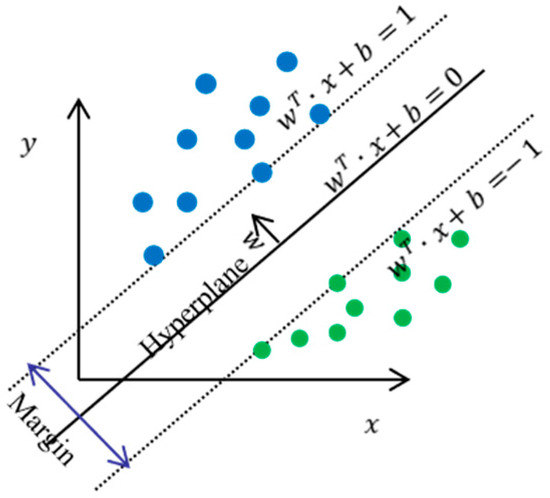
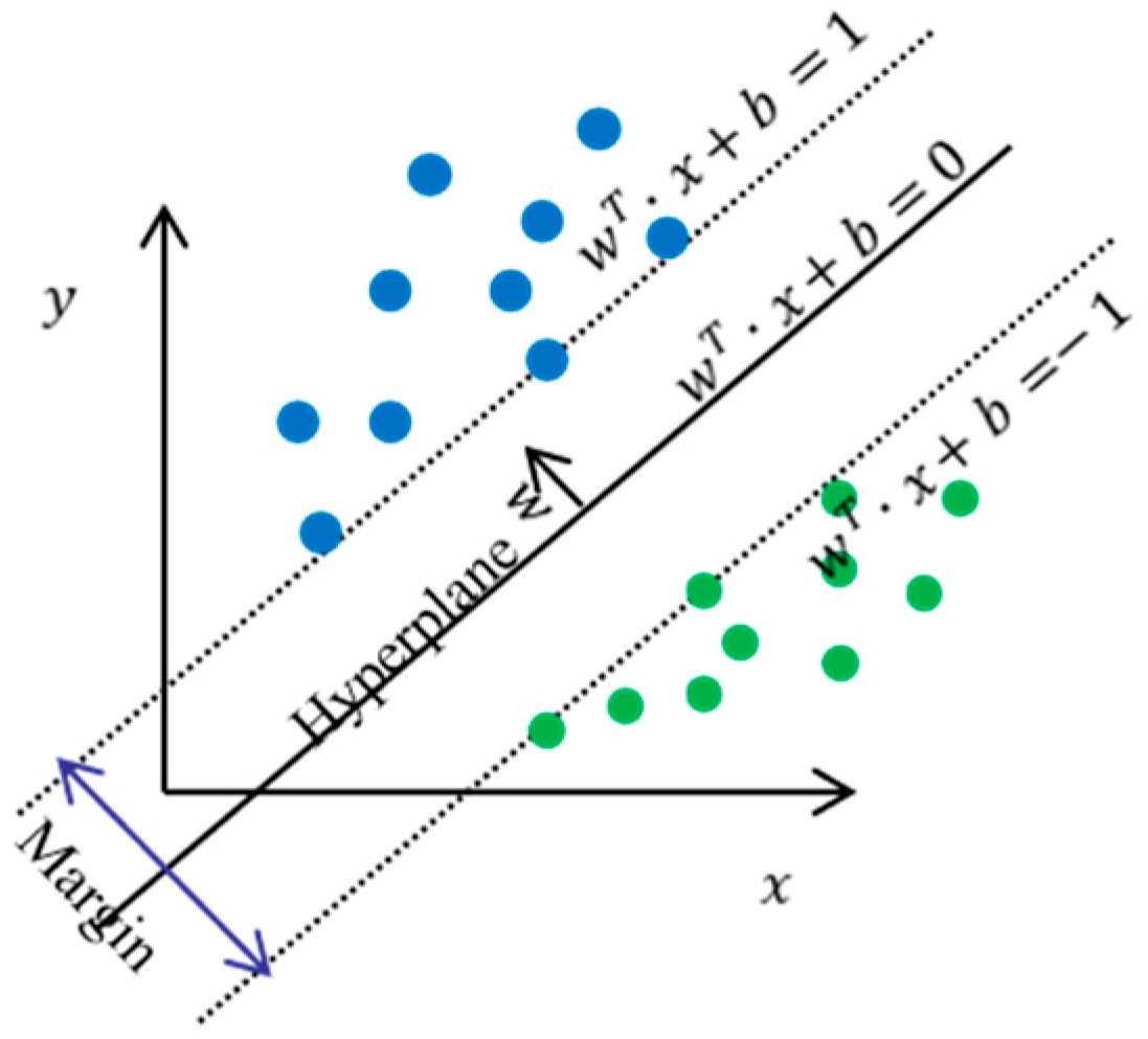
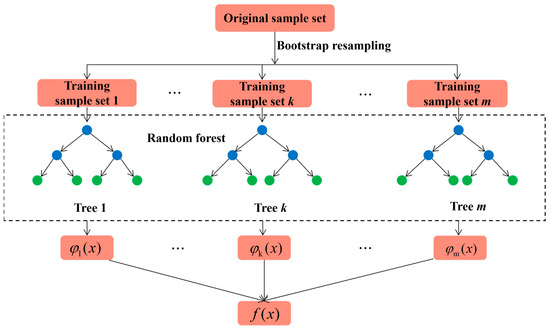
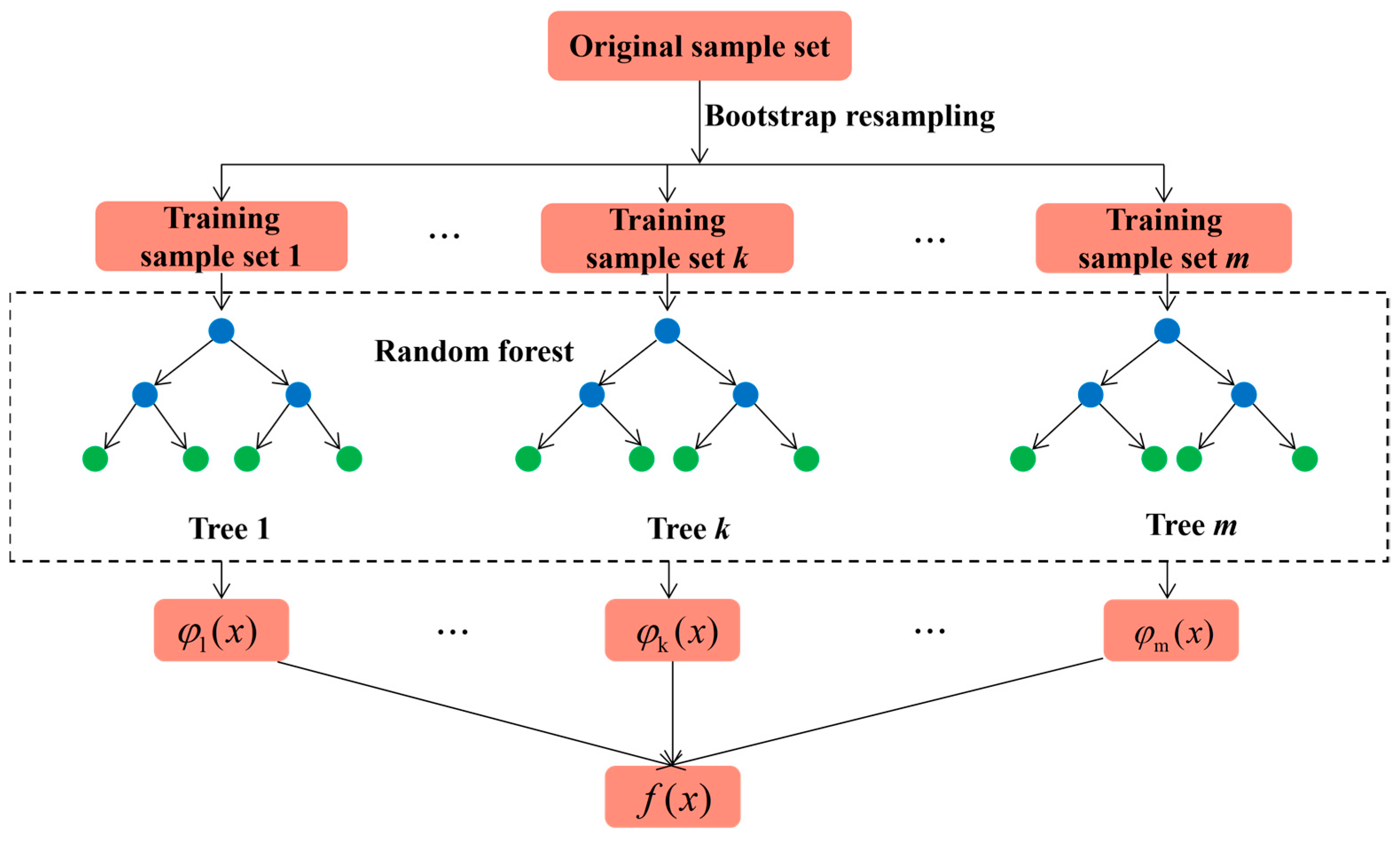
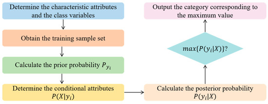
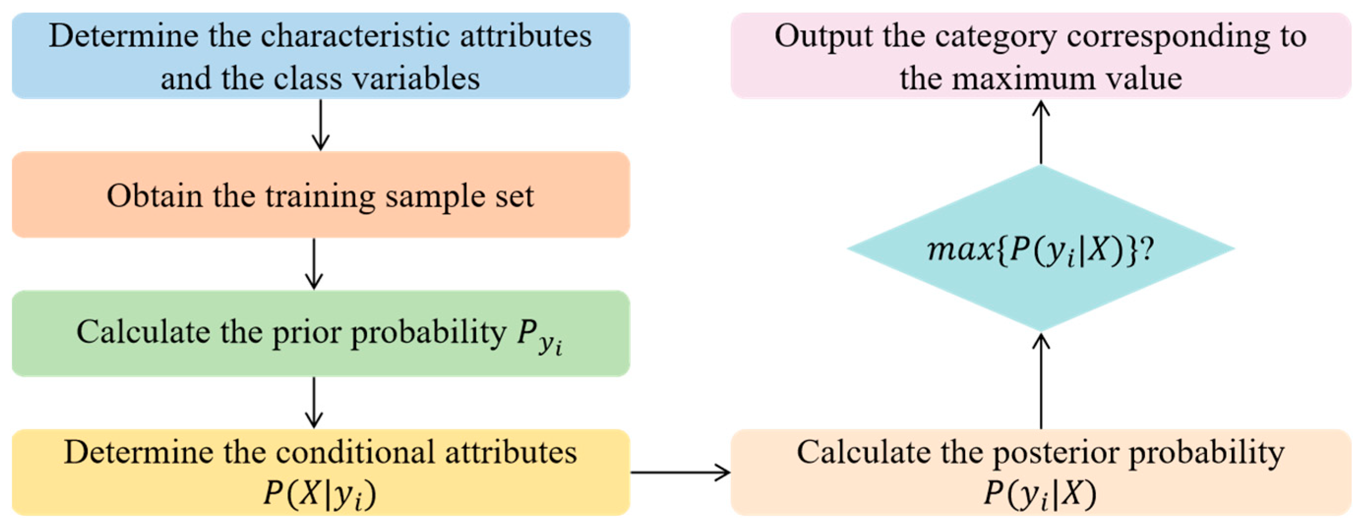
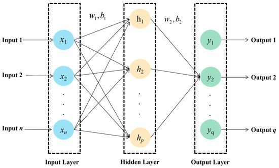
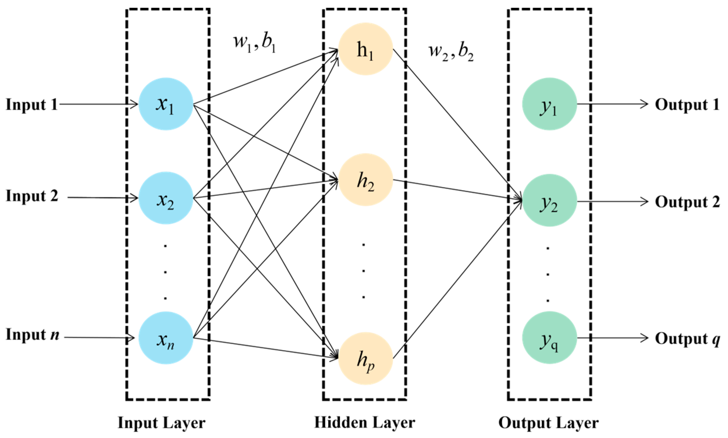
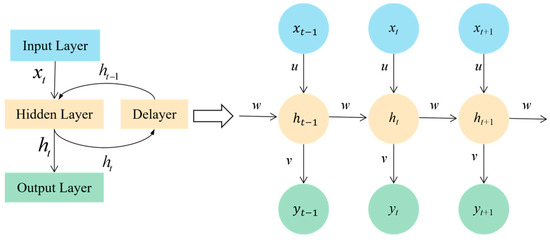
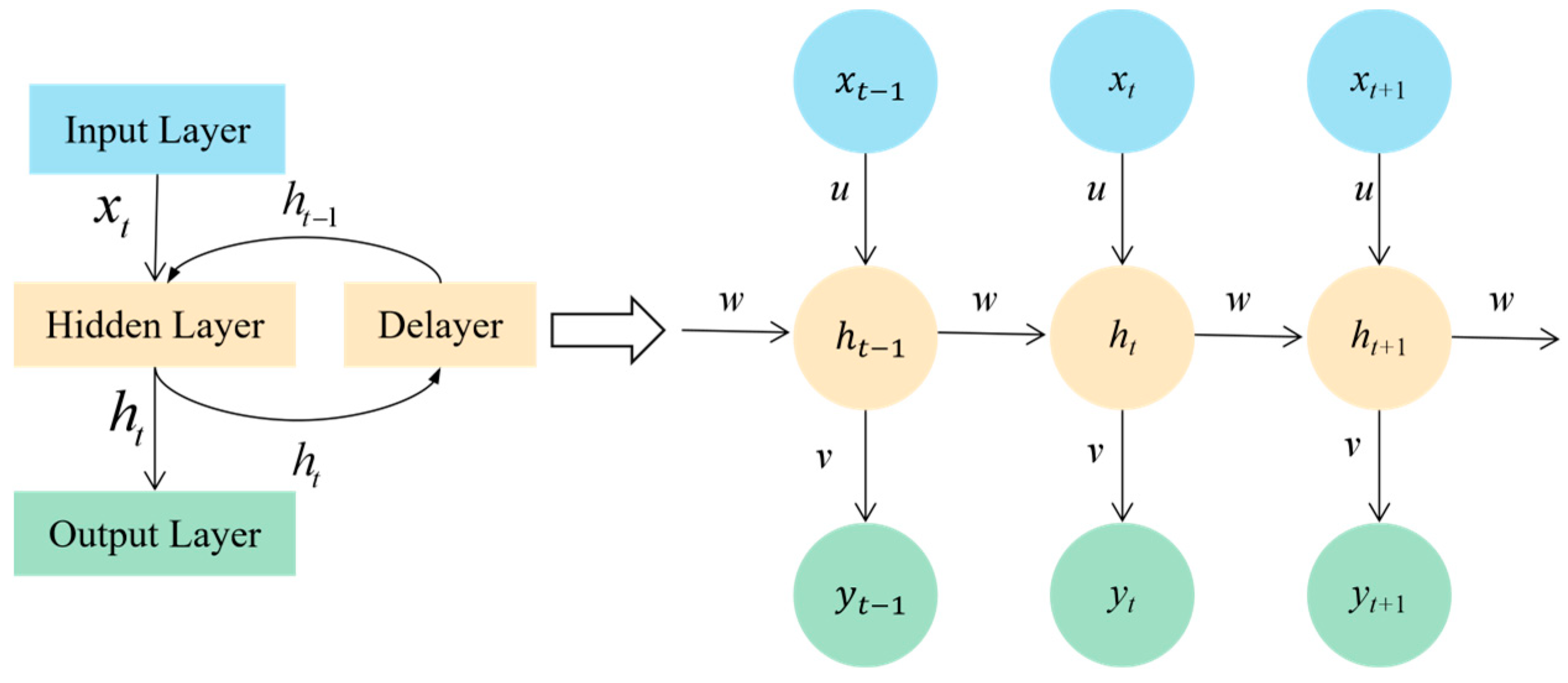
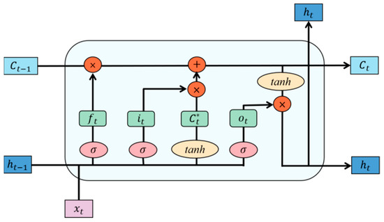
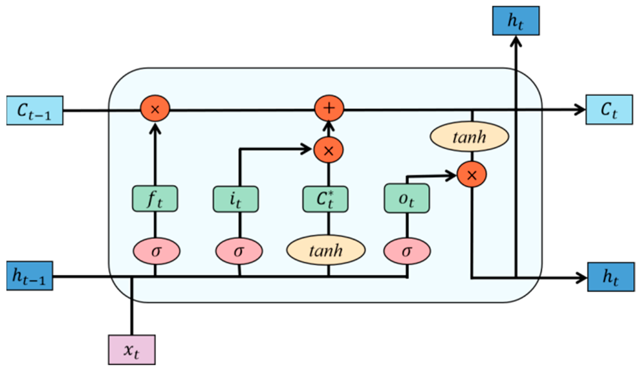
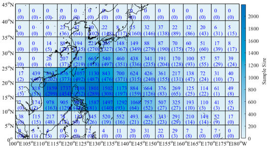
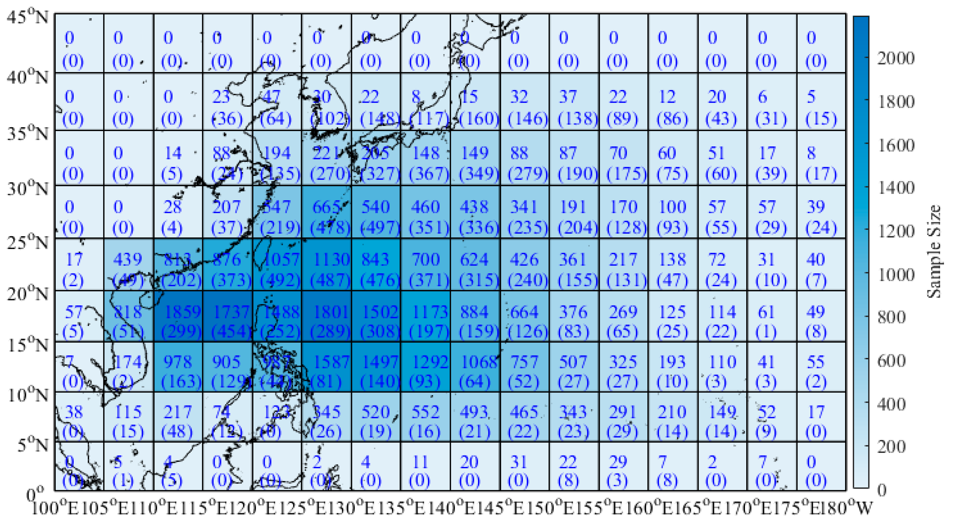
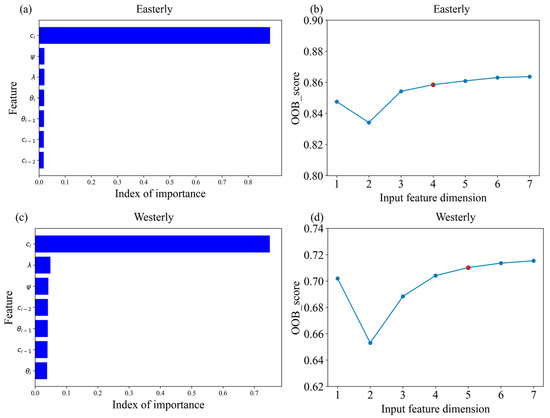
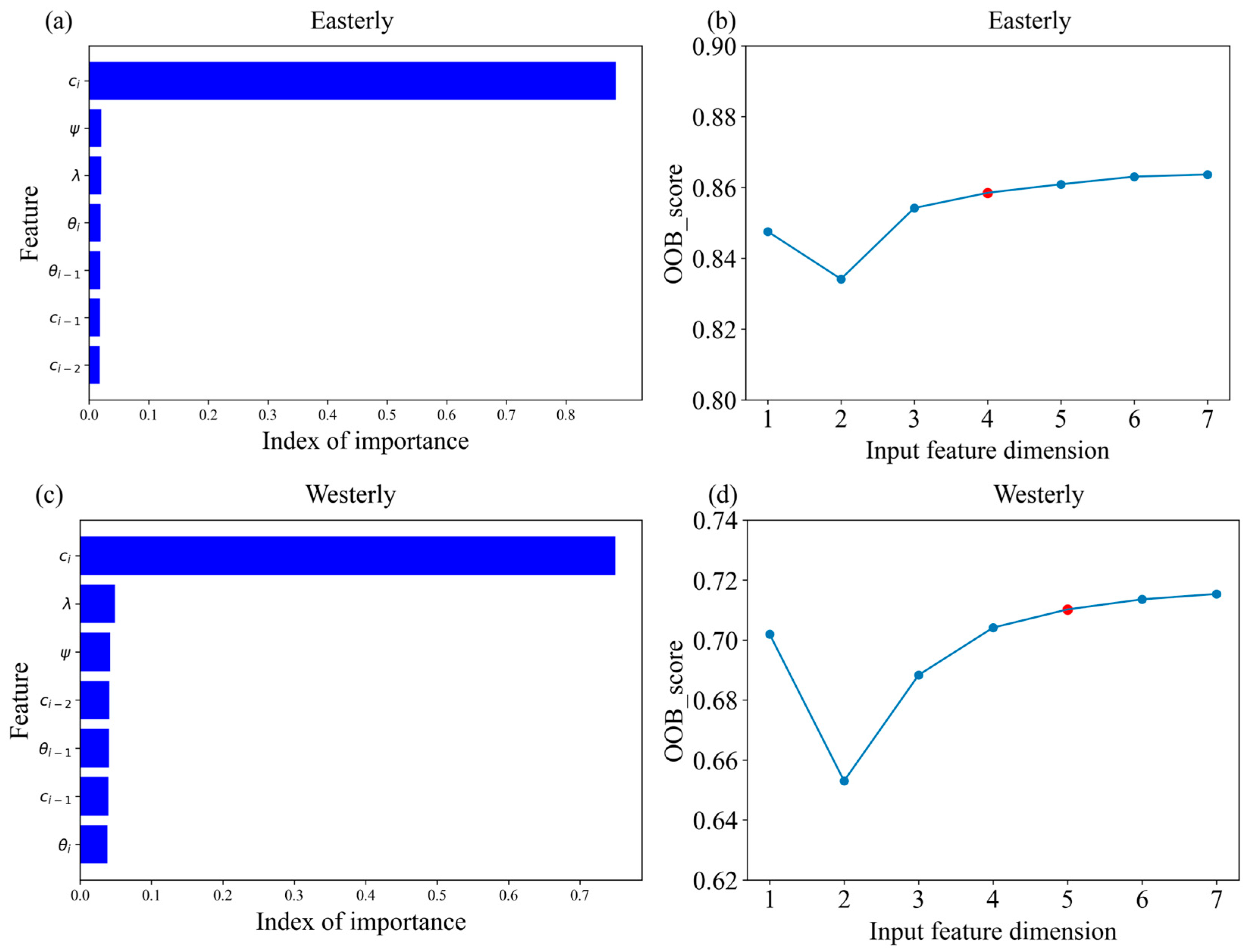
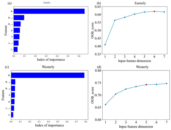
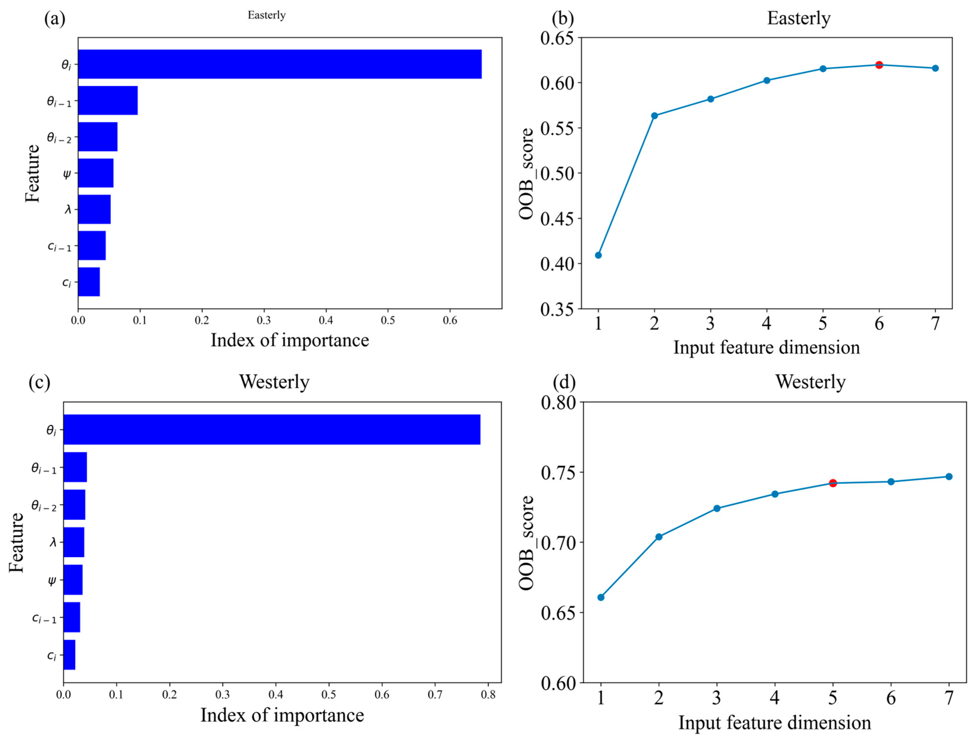
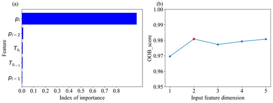
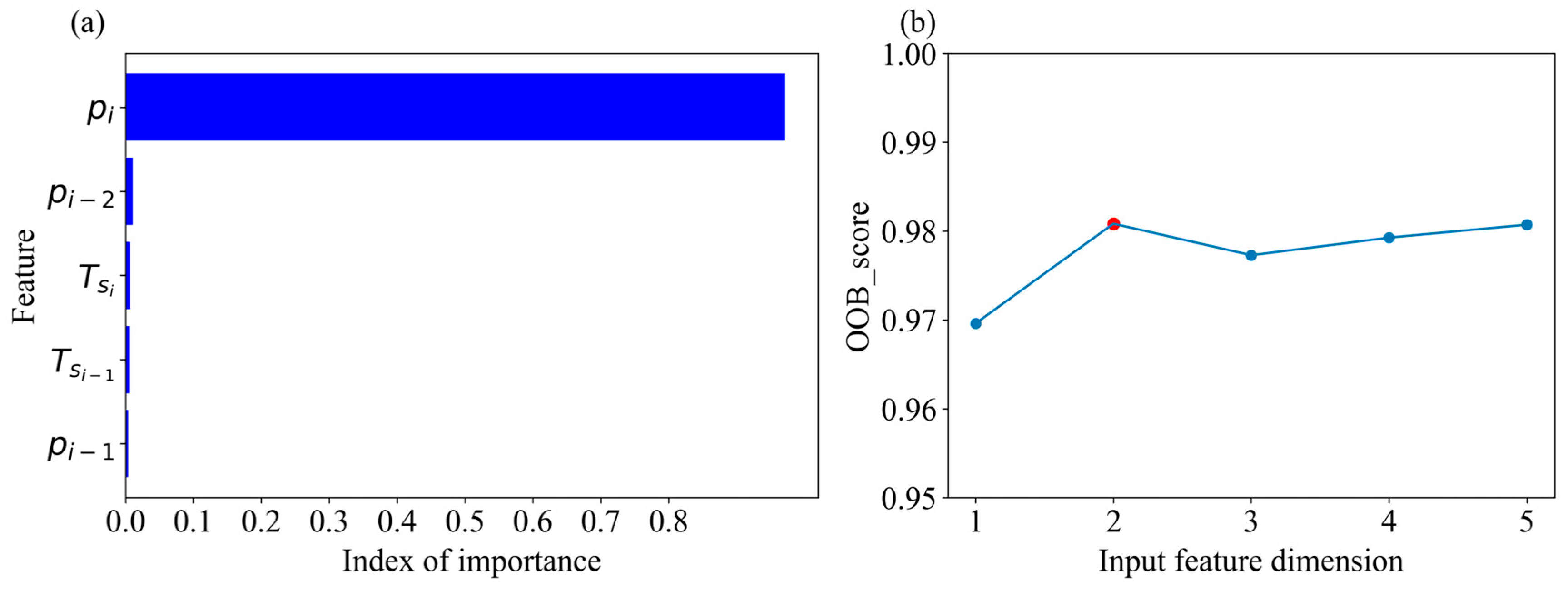
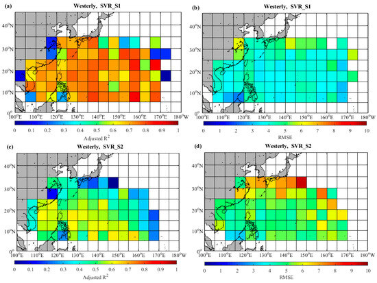
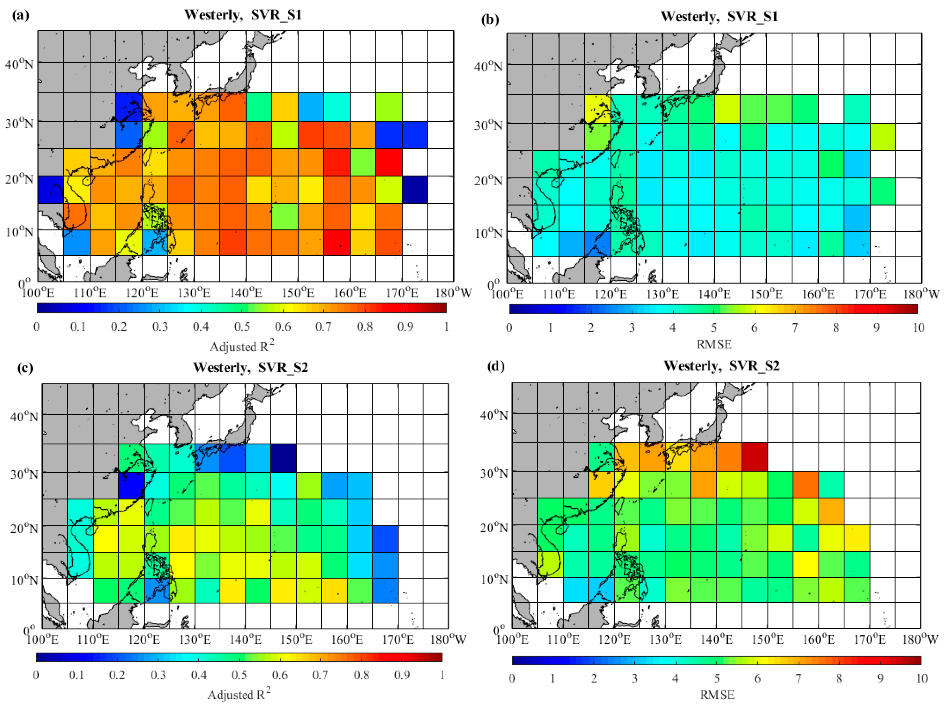
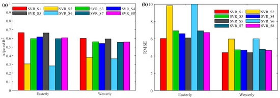
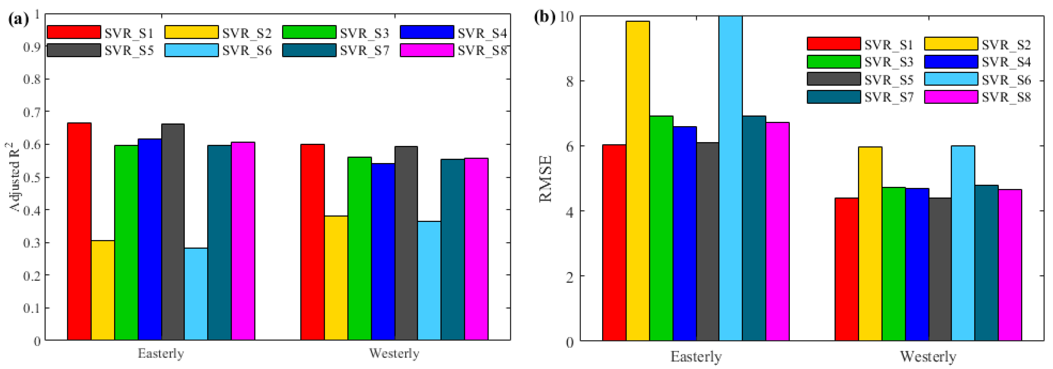
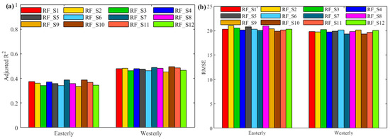
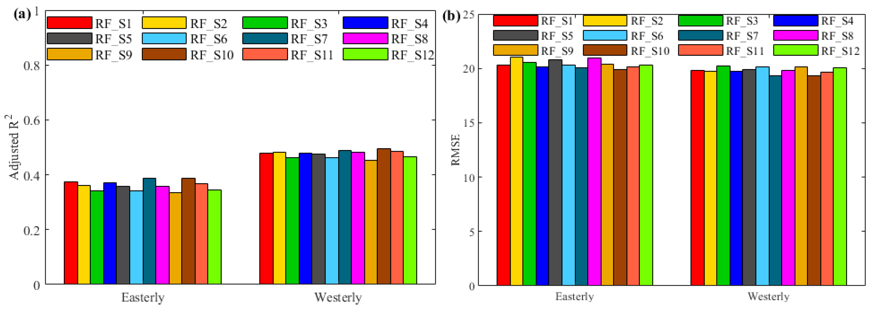
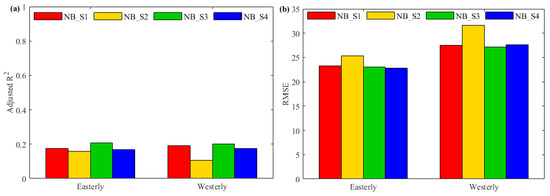
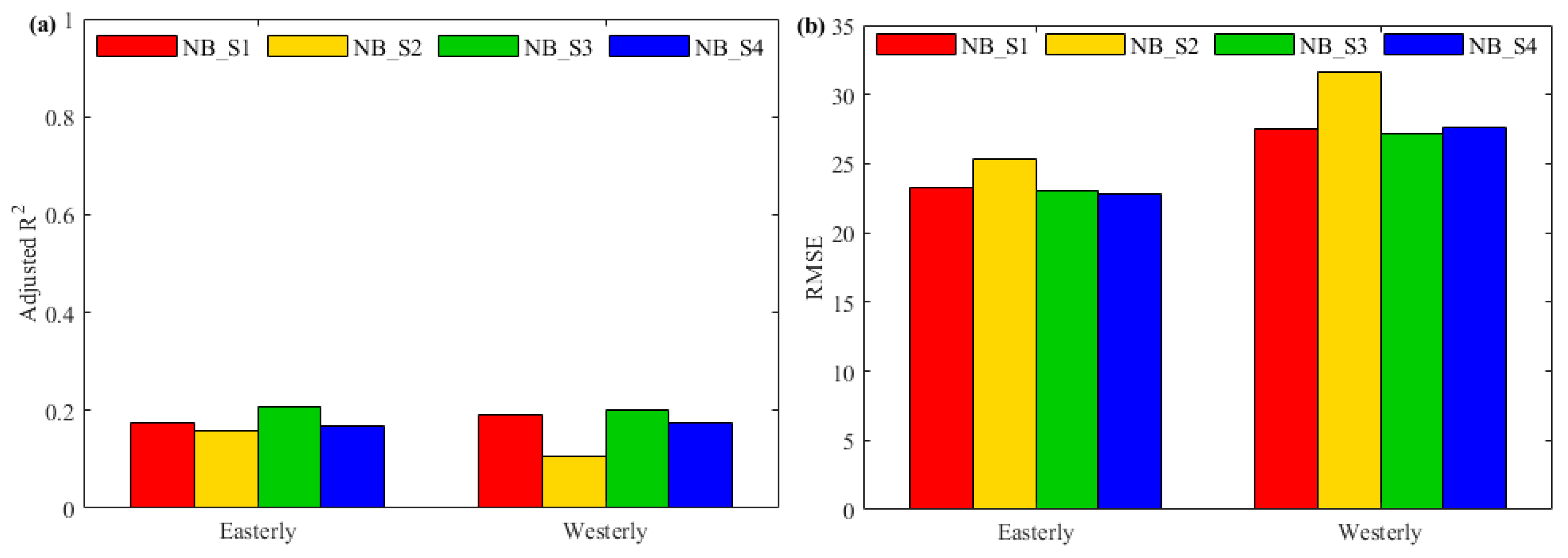
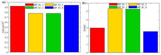
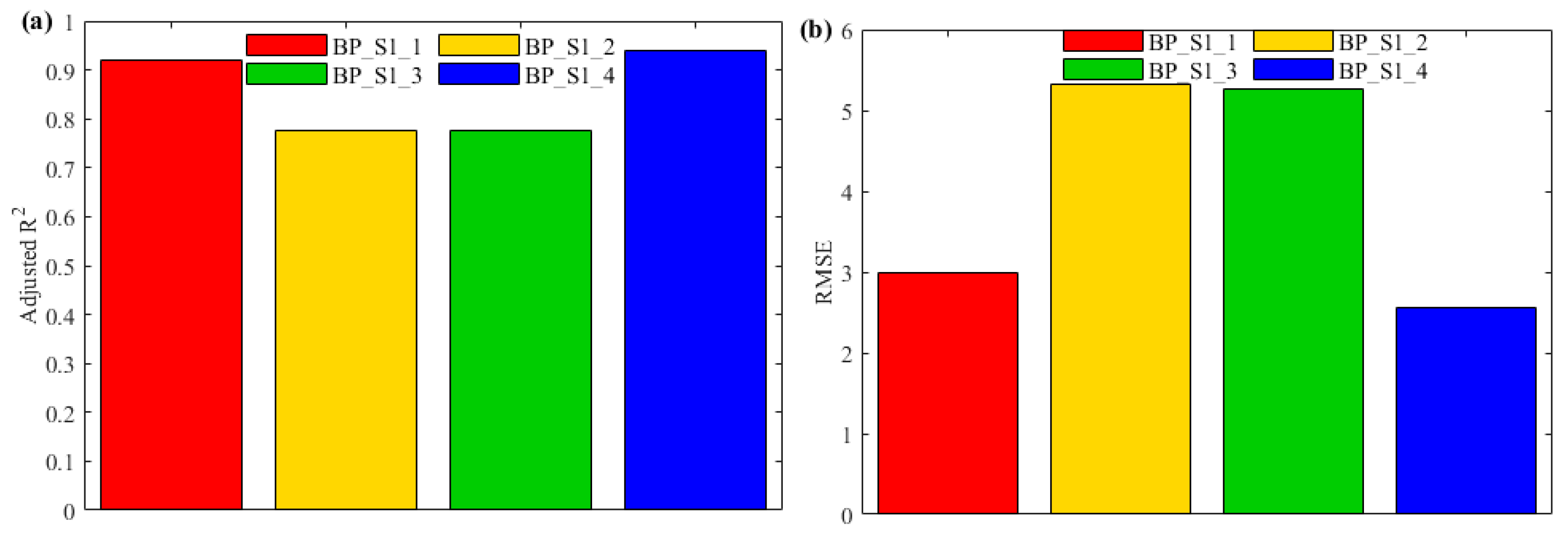
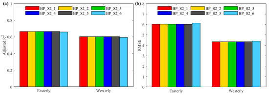
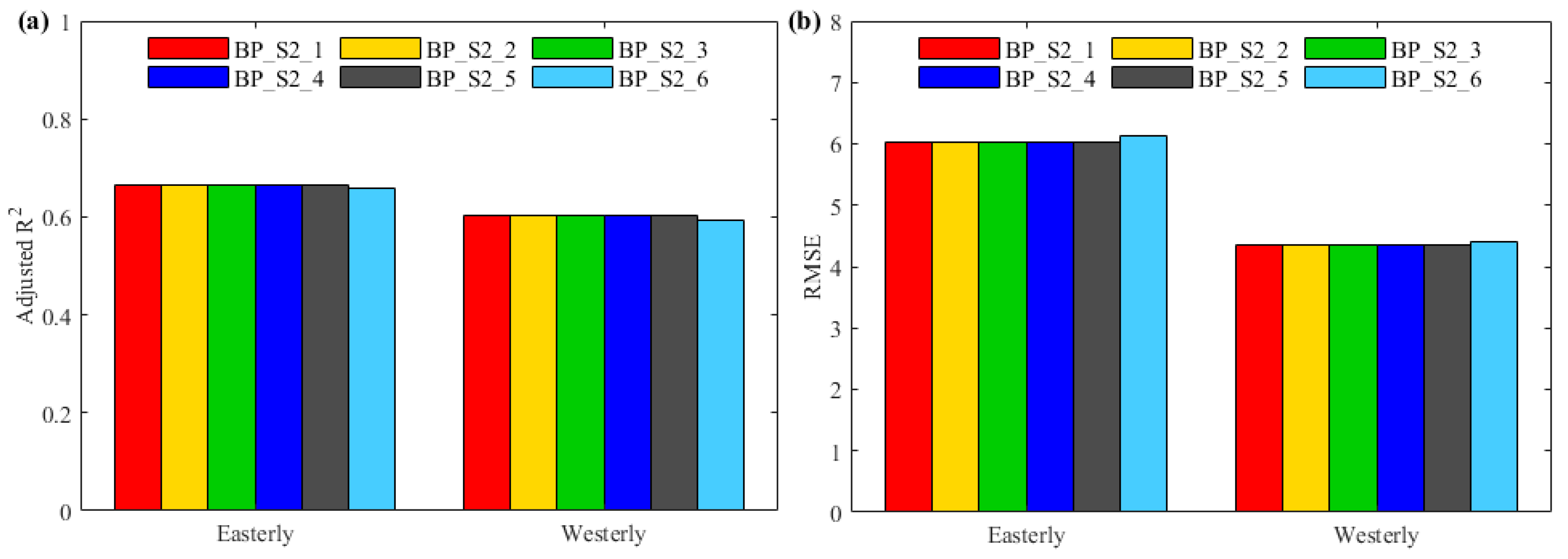
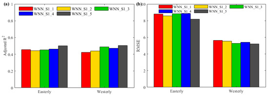
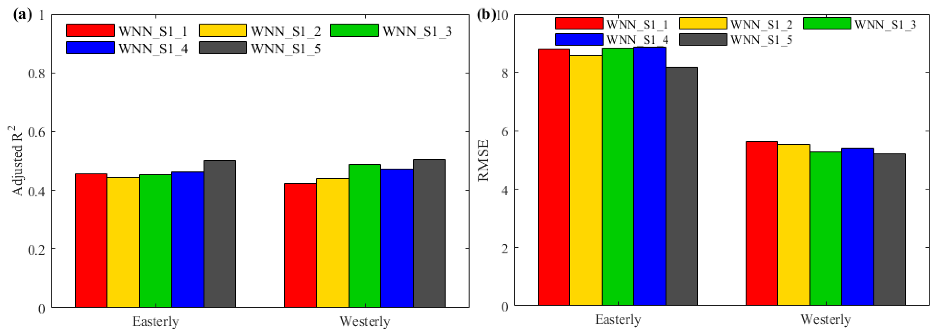
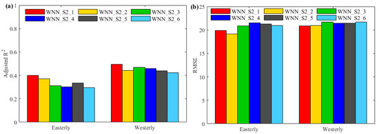
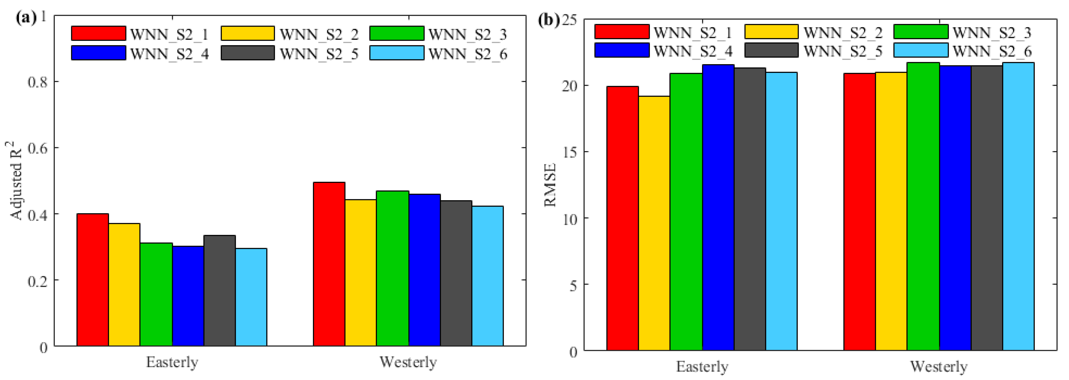
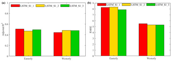
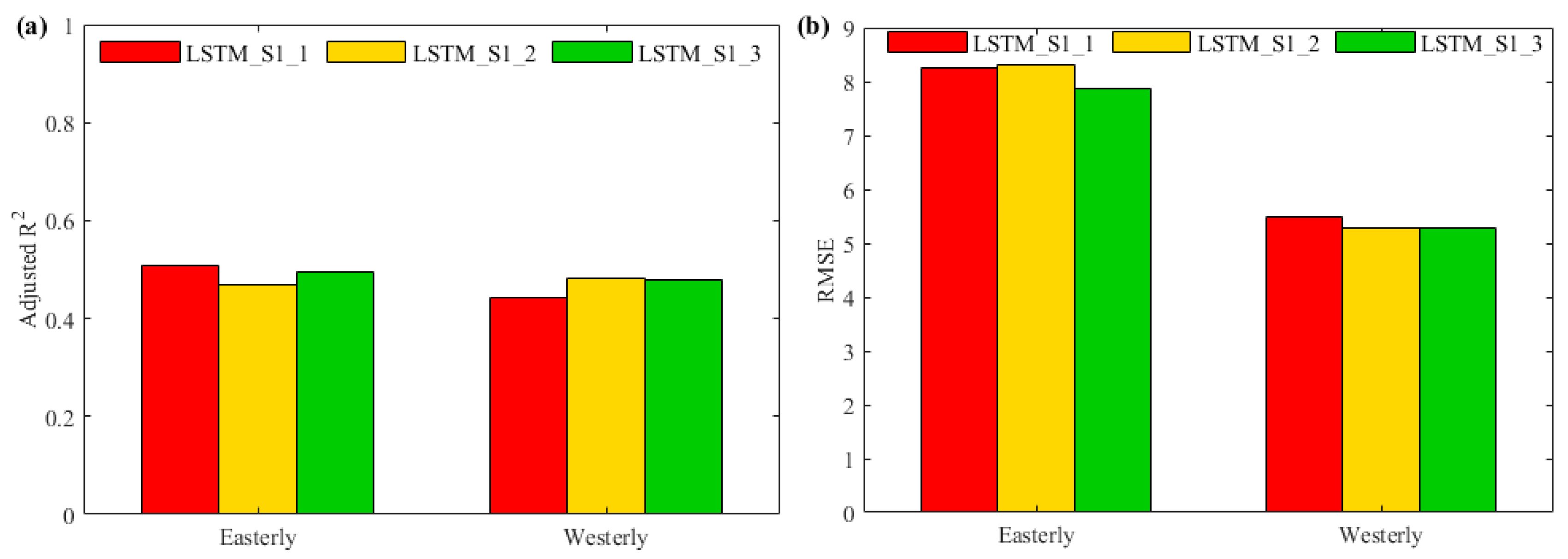
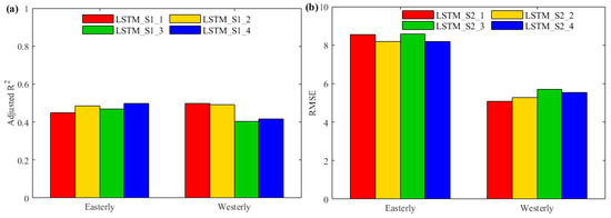
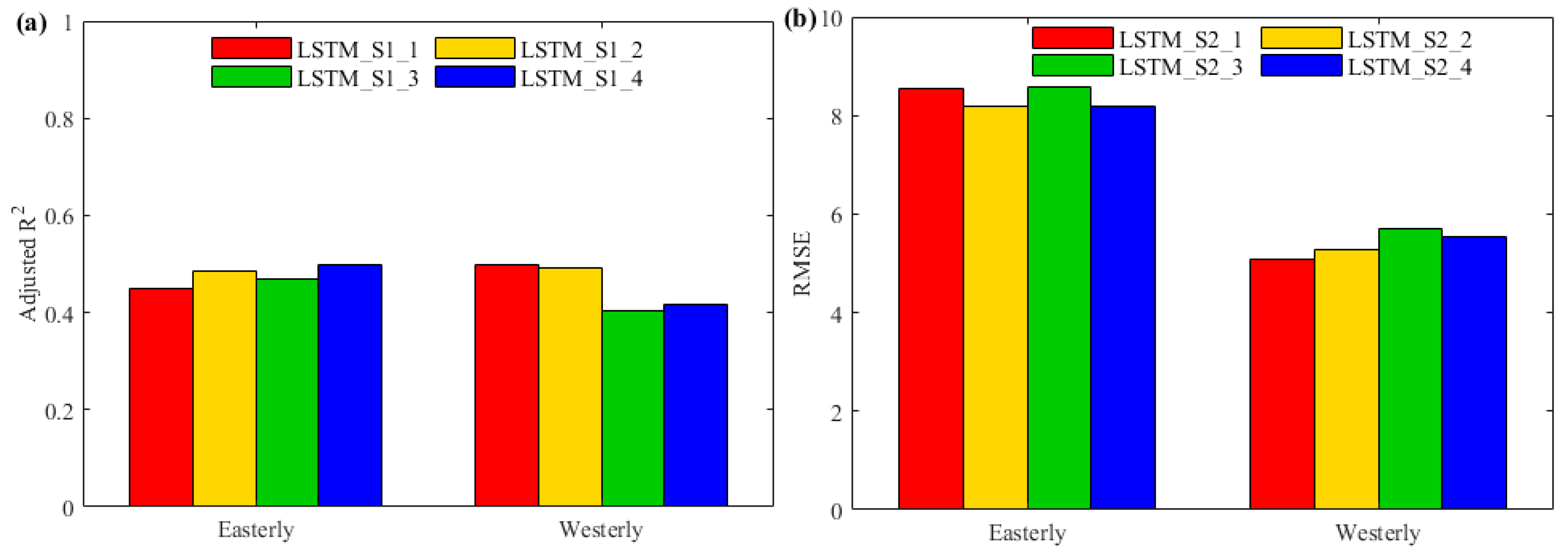
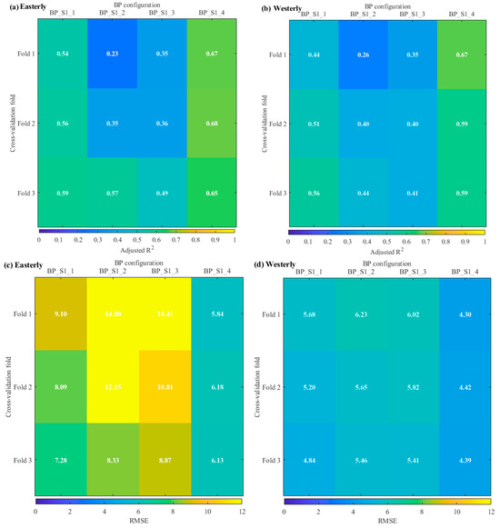
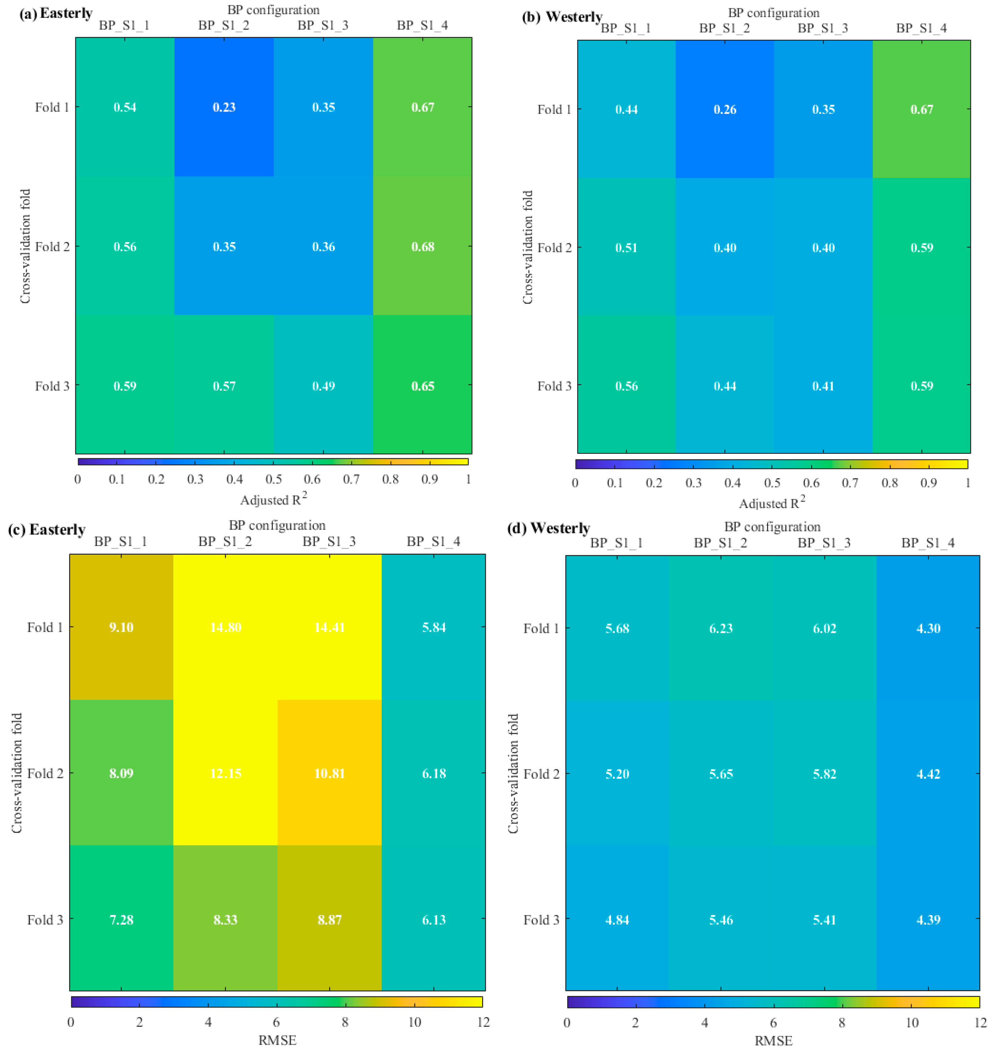
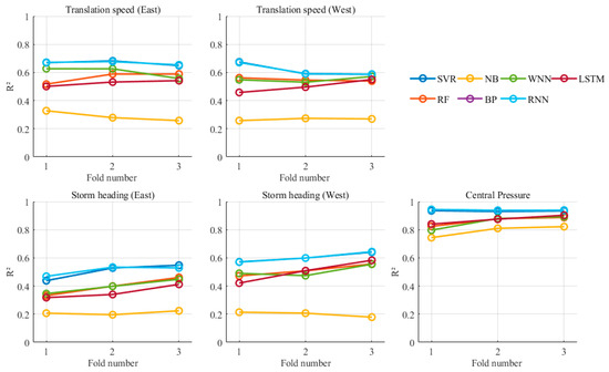
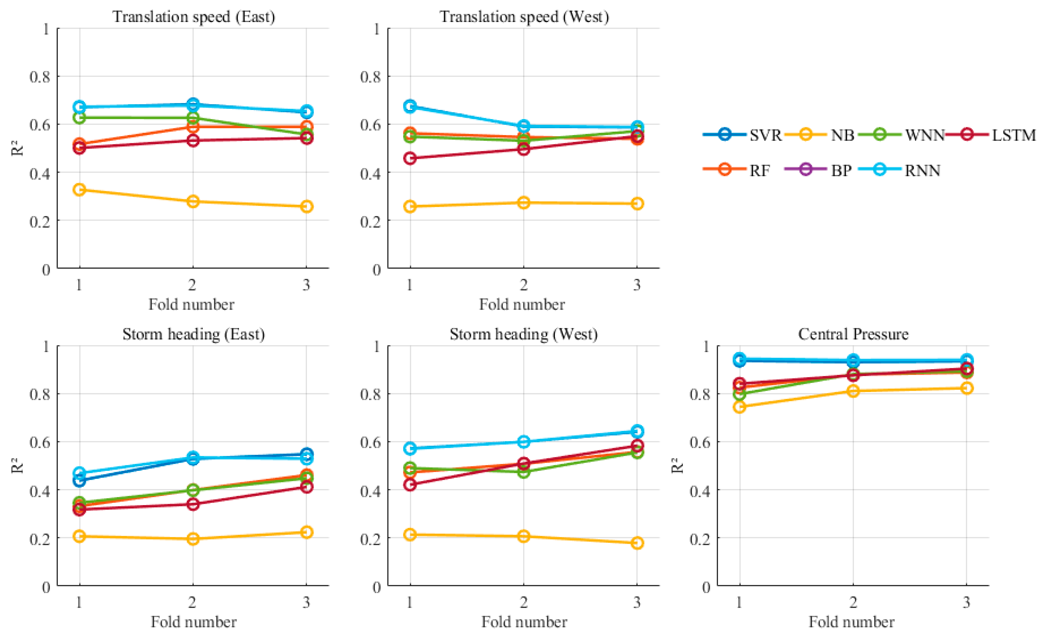
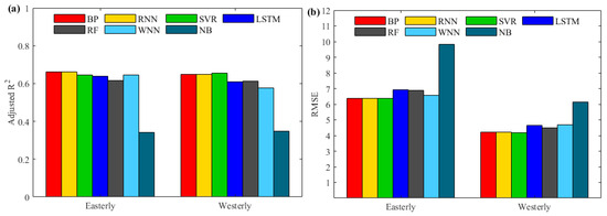
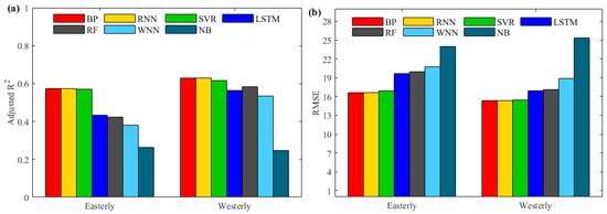
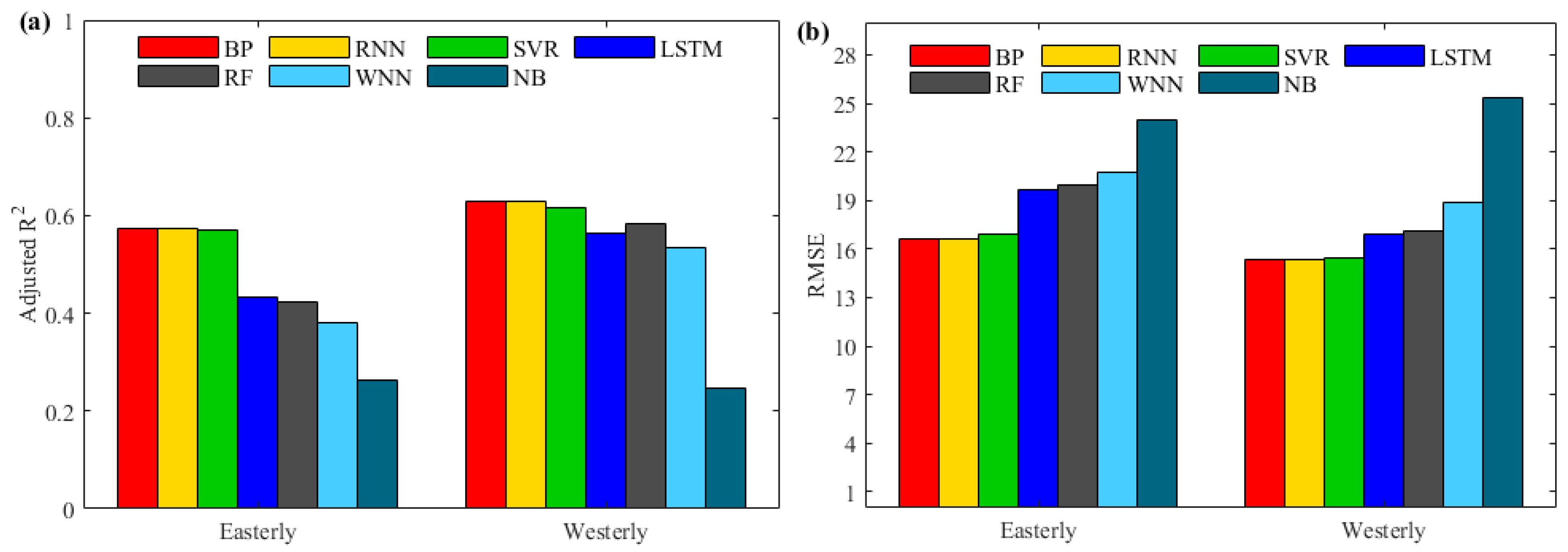
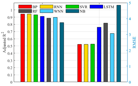
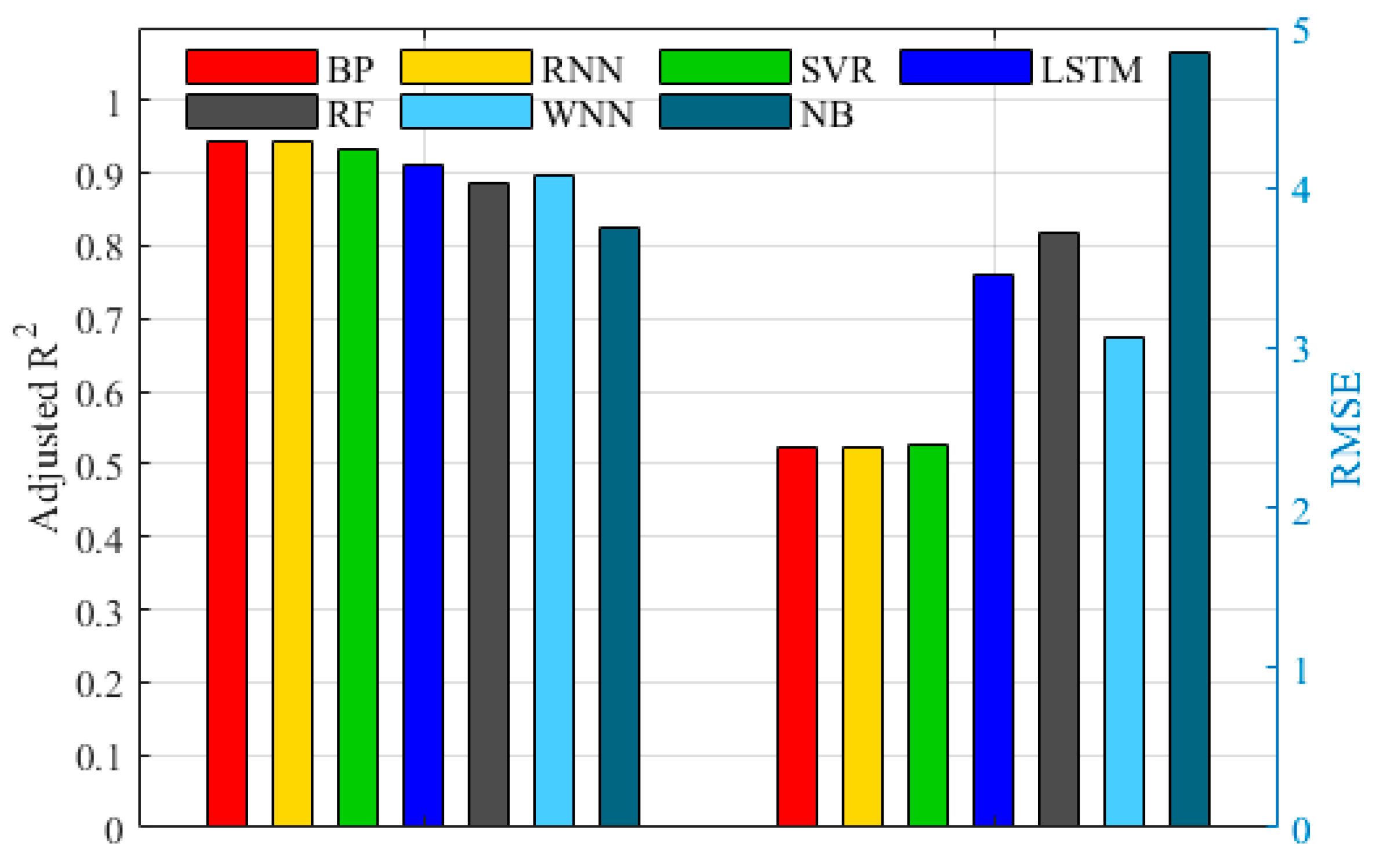
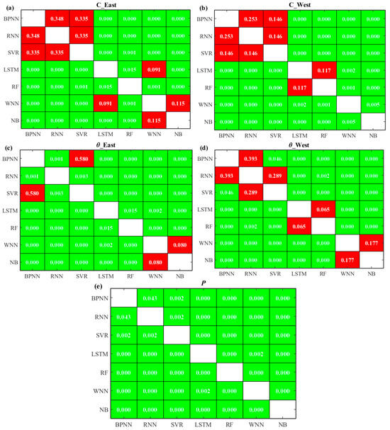
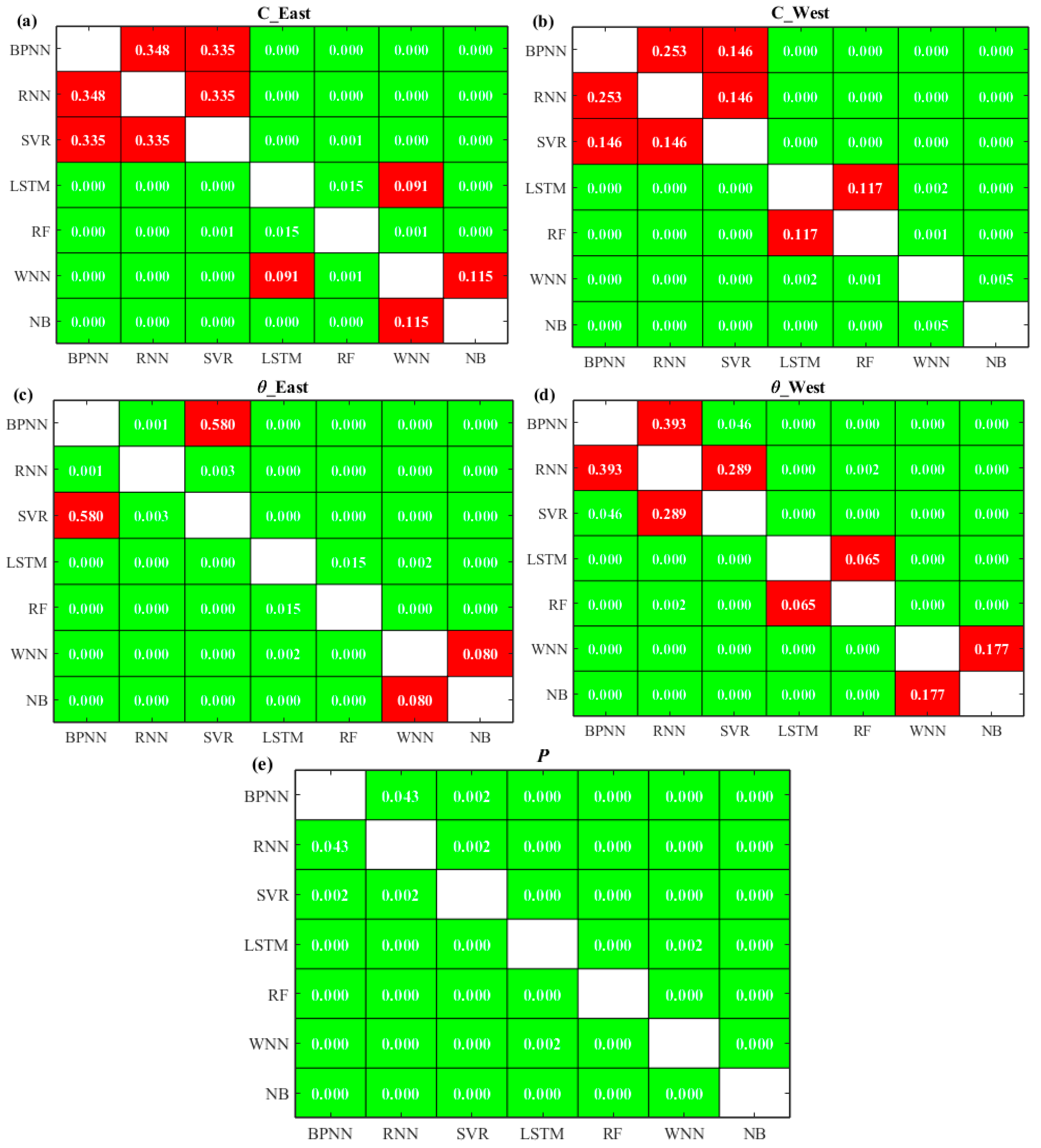
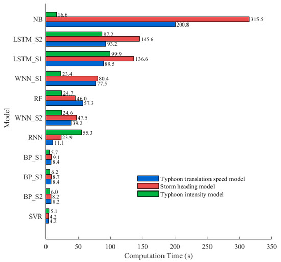
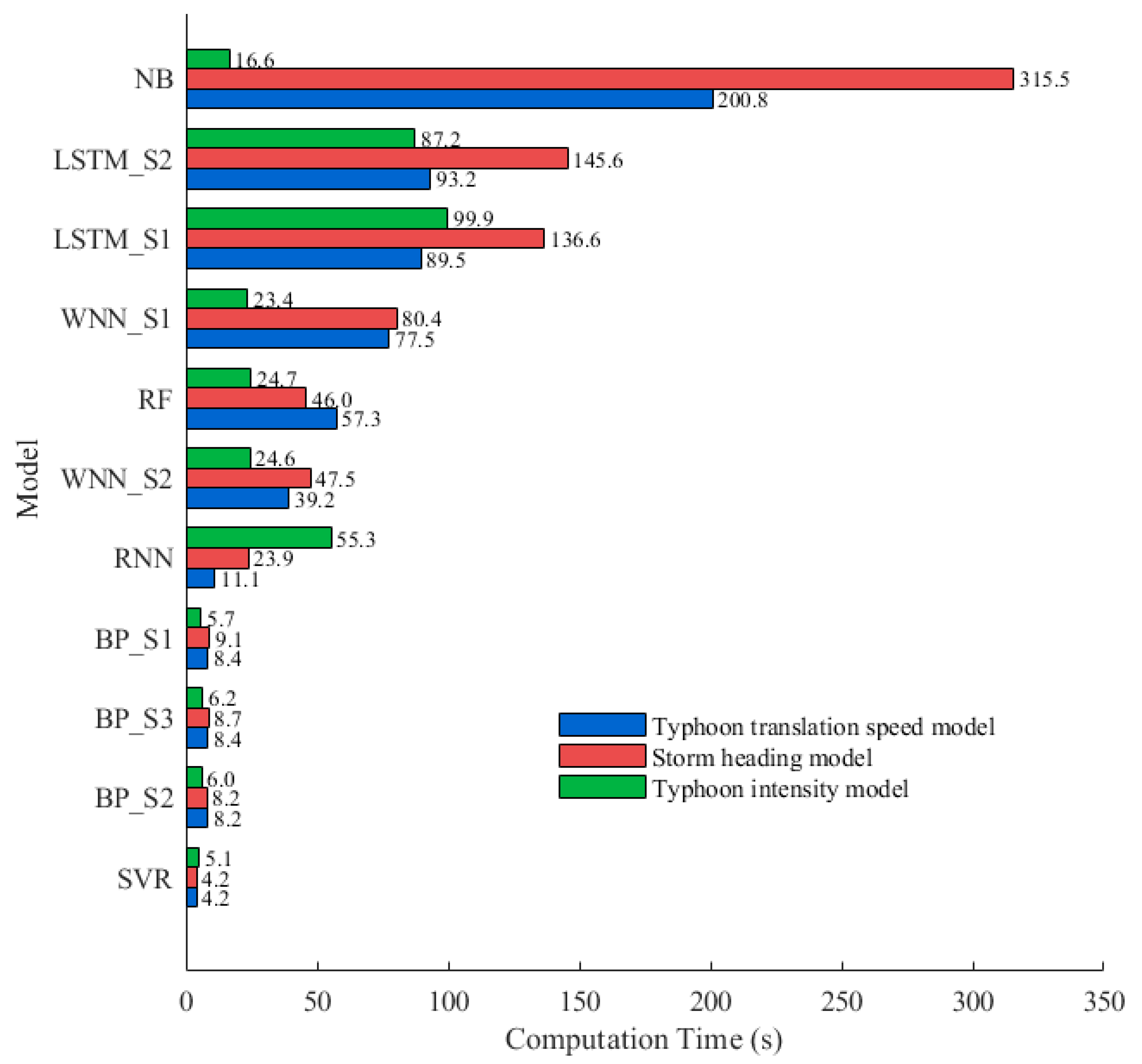
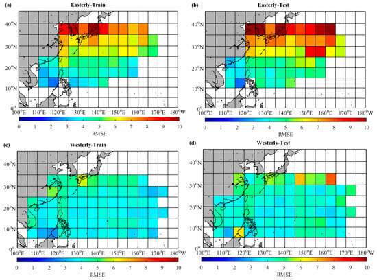
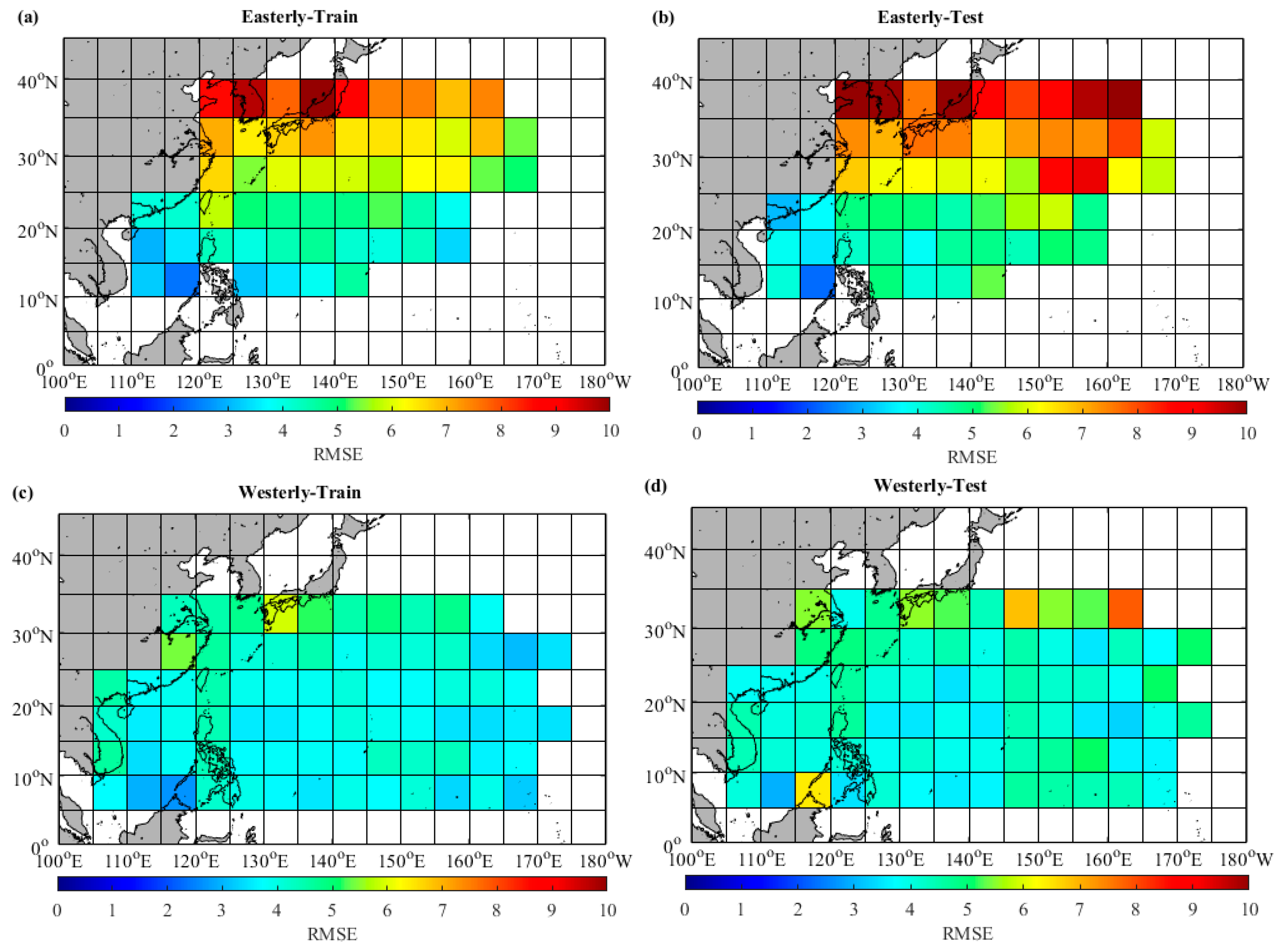
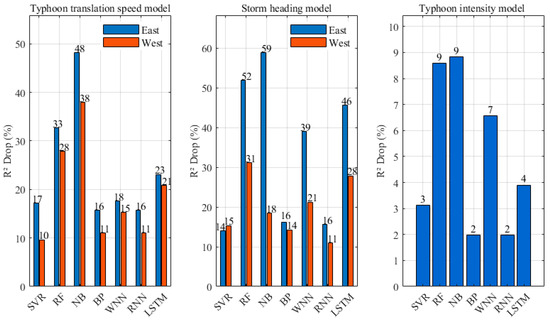
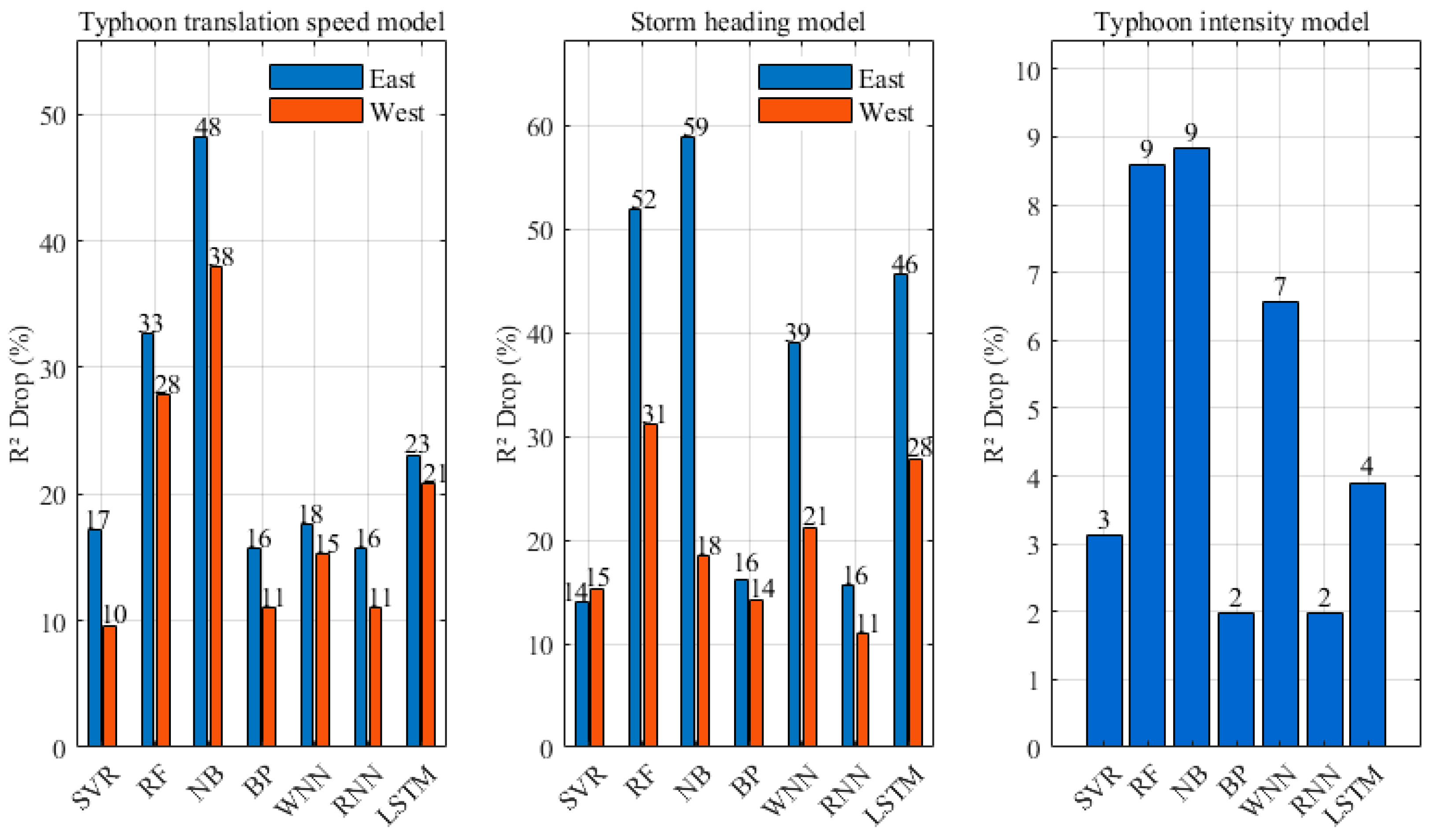
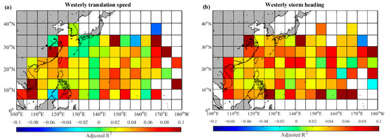
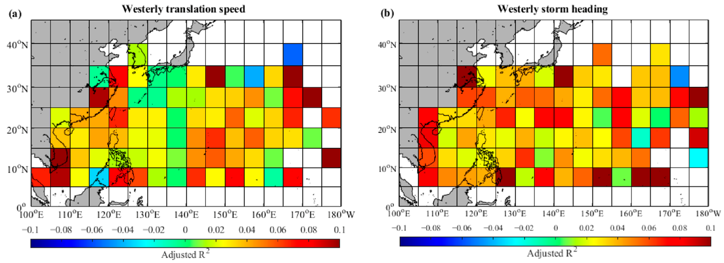
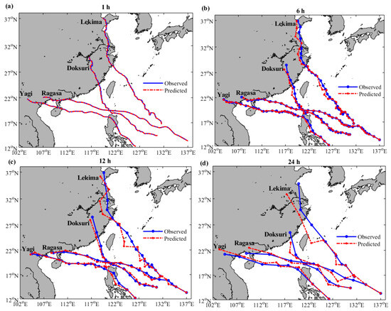
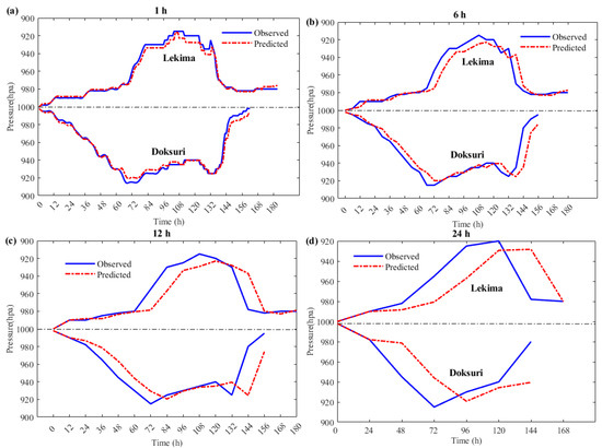

Disclaimer/Publisher’s Note: The statements, opinions and data contained in all publications are solely those of the individual author(s) and contributor(s) and not of MDPI and/or the editor(s). MDPI and/or the editor(s) disclaim responsibility for any injury to people or property resulting from any ideas, methods, instructions or products referred to in the content. |
© 2026 by the authors. Licensee MDPI, Basel, Switzerland. This article is an open access article distributed under the terms and conditions of the Creative Commons Attribution (CC BY) license.