


Abstract
Cavitation is a common phenomenon in naval and ocean engineering, typically occurring in the wakes of high-speed rotating propellers and on the surfaces of fast-moving underwater vehicles. To investigate cavitation phenomena, computational fluid dynamics (CFD) simulations are indispensable. Nevertheless, the inherently complex nature of cavitation, which involves phase transitions, heat transfer, and significant pressure fluctuations, often results in high computational costs for these simulations. To address the computational challenges associated with cavitation simulations, a DeepCFD model, which leverages convolutional neural networks (CNNs), was employed to accurately predict cavitation around hydrofoils. Through specific modifications, the DeepCFD model was trained on 400 hydrofoil configurations, learned from CFD simulations. The numerical methods were validated against a modified NACA66 hydrofoil. It was found that the model could accurately predict cavitation shapes under various flow conditions, although it showed some discrepancies in velocity predictions, especially for detached cavitating flows. The significance of this study lies in its potential to simply predict cavitating flows and expedite marine vehicle design through the application of CNNs in cavitation prediction, offering a novel and impactful approach to computational fluid dynamics in the field.
1. Introduction
Cavitation is characterized by abrupt phase transitions, heat transfer, significant pressure fluctuations, and transient pressure spikes, which result in substantial density variations between the liquid and vapor phases within the flow field. Extensive experimental investigations have been conducted to elucidate cavitation phenomena by analyzing various cavitation structures. These studies have highlighted the role of cavitation instability in noise generation and material erosion [1,2]. Despite these advancements, the underlying mechanisms governing these phenomena remain incompletely understood.
Numerical methods, particularly CFD, have been effectively employed to assess the hydrodynamic performance of propellers, including cavitation analysis [3,4,5]. Gaggero et al. [6] concentrated on predicting the inception of tip vortices, while Yilmaz et al. [7] utilized advanced grid adaptation and refinement techniques for cavitation simulations. Viitanen et al. [8] investigated cavitation phenomena on both model- and full-scale marine propellers, as well as in more realistic propeller installations. Ng’aru and Park [9] explored cavitation flows around marine propellers using a range of flow solvers, including incompressible, isothermal compressible, and fully compressible models. Numerous experts and scholars have utilized CFD to conduct research on cavitation, gaining a deeper understanding of the formation and development of cavitation phenomena, and thereby making simulation results more closely aligned with real-world conditions.
Although CFD solvers are capable of generating highly accurate results, their substantial computational resource requirements render them expensive, and the extended time needed to obtain solutions can hinder extensive iterative design processes. Consequently, data-driven machine learning methods, which approximate these simulations with high accuracy and significantly reduced computational costs, have become particularly attractive [10]. The rapid advancements in computational tools and optimization models have led to considerable improvements in machine learning techniques [11]. Methods such as artificial neural networks and convolutional neural networks have increasingly been employed to tackle complex problems [12,13]. The literature on CFD data-driven approaches has significantly contributed to the development of machine learning models for fluid flow prediction. Moreover, recent studies have extended these applications to broader domains, including physics-informed neural networks, hydrofoil design optimization, and the acceleration of sparse linear system solutions [14,15].
In this study, DeepCFD, a deep learning model utilizing a convolutional neural network (CNN) architecture, was employed to predict distributions of velocity, pressure, and water phase. The development of the DeepCFD model involved conducting high-fidelity CFD simulations on 400 different hydrofoils. The selection of hydrofoils encompassed a wide range of geometries and operational conditions. The resulting CNN model is not only highly accurate but also broadly applicable to various hydrodynamic scenarios. The DeepCFD model’s architecture was carefully designed to capture the intricate relationships between hydrofoil sections, flow conditions, and the resulting cavitation. Therefore, the model provided a robust tool for predicting cavitation patterns with reduced computational costs. These CFD computations were executed using OpenFOAM 10 [5,9,16].
2. Computational Methods
In this study, the open-source CFD library platform OpenFOAM was utilized [5,17]. For the simulation of cavitation, the interPhaseChangeFoam solver was selected [9], which incorporates common assumptions such as incompressibility and immiscibility. The governing equations include the incompressible conservation equations for mass and momentum, as well as the advection equation for the volume fraction. These equations are expressed as follows:
In these equations, , , , and represent the velocity, pressure, volume fraction, and source term for water generation, respectively. The subscripts (i, j, k) denote the x, y, and z directions in Cartesian coordinates. The volume fraction advection equation, as formulated by Hirt and Nichols [18], is used to compute the volume fraction of water. In this context, α = 1 and α = 0 denote regions of 100% water and 100% vapor, respectively. In regions near the phase interface, the volume fraction α varies between 0 and 1.
To close the RANS equation, a k- SST turbulence model was employed. This model incorporates the k-ε turbulence model [19] (). makes a smooth transition between the two near walls and in the free stream region. The k-ω SST model calculates turbulent viscosity with an additional viscosity limiter, which improves agreement with experimental measurements of separated flows. It is widely accepted as an industry standard turbulence model due to its high accuracy and cost-effectiveness, particularly in predicting flow separation and behavior under adverse pressure gradients [20]. The equations for turbulent kinetic energy () and specific dissipation rate () are presented below [21]:
where eddy viscosity , a1 is the experimental constant with the value 0.31, is 1.0, S is the strain rate magnitude, and is the blending function . . The turbulence constants are: and .
Given its widespread application in the field of hydrofoil cavitation, the cavitation model proposed by Schnerr and Sauer [22] is adopted in this study. In this model, mass transfer between phases is governed by the difference between the saturated pressure () and the local pressure (). The mass transfer within the liquid phase is characterized by the growth of the liquid mass, which is primarily driven by vapor condensation and liquid evaporation. The rates of condensation and evaporation are defined as follows [9]:
In these equations, ρv and ρl represent the vapor and liquid densities, respectively, while CC and CV denote the condensation and evaporation coefficients; here, = = 0.2. The nucleation fraction () is defined as , where . The model’s input parameters include the nucleus density ( = 1.6 × 10⁹) and the initial nucleus diameter ( = 2.0 × 10⁻⁸).
3. DeepCFD Model
Traditional CFD methods, while capable of generating relatively accurate results, often face significant challenges due to high computational costs and extended solution times. The DeepCFD model has been employed to address these limitations [23,24]. DeepCFD utilizes deep convolutional neural networks (DCNNs) to develop surrogate models that accurately predict physical phenomena. In this study, the DeepCFD model is applied to forecast cavitation phenomena on hydrofoils and to provide efficient solutions for predicting velocity and pressure.
Convolutional neural networks (CNNs) have demonstrated a robust ability to learn critical features from pixel-level images, making them particularly effective for classification and regression tasks [25,26]. Compared to traditional fully connected neural networks, CNNs offer additional advantages through convolutional operations that facilitate weight sharing and sparse connections. These attributes enable CNNs to use memory more efficiently and extract the essential information necessary for the development of surrogate models. Such models are capable of accurately approximating complex regions, including entire cavitation zones, as well as the associated velocity and pressure fields.
3.1. Input Data
The input files for the DeepCFD model are designated dataX and dataY. The cavity pattern on a hydrofoil surface is primarily influenced by the hydrofoil’s geometry and angle of attack (AoA). The dataX file contains input information related to the geometry of various hydrofoils. As a data-driven approach, deep learning leverages extensive datasets to capture complex relationships between inputs and outputs. By utilizing a large volume of data samples, deep learning models can effectively learn and generalize underlying patterns and features, enabling them to perform well with new data. Consequently, the dataY file comprises the CFD solutions for velocity (), pressure (), and water phase () obtained from the selected solver.
The input layer of the convolutional neural network (CNN) model must incorporate both geometric information and the AoA to accurately capture the physical characteristics of the problem. In this study, the DeepCFD model utilizes the signed distance function (SDF) for this purpose [23]. The SDF measures the distance from each point in the CFD mesh to a specified surface, enabling the model to effectively encode geometric features. The signed distance function is defined by the following equation:
where is a subset of a metric space (, ) and denotes the boundary of . For any
where denotes the infimum. The signed distance function assigns negative distances to grid positions located inside the obstacle’s interior, denoted by . This approach enables the model to distinguish between points inside and outside the geometric boundaries, thereby enhancing the representation of the physical domain within the CNN framework.
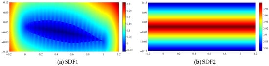
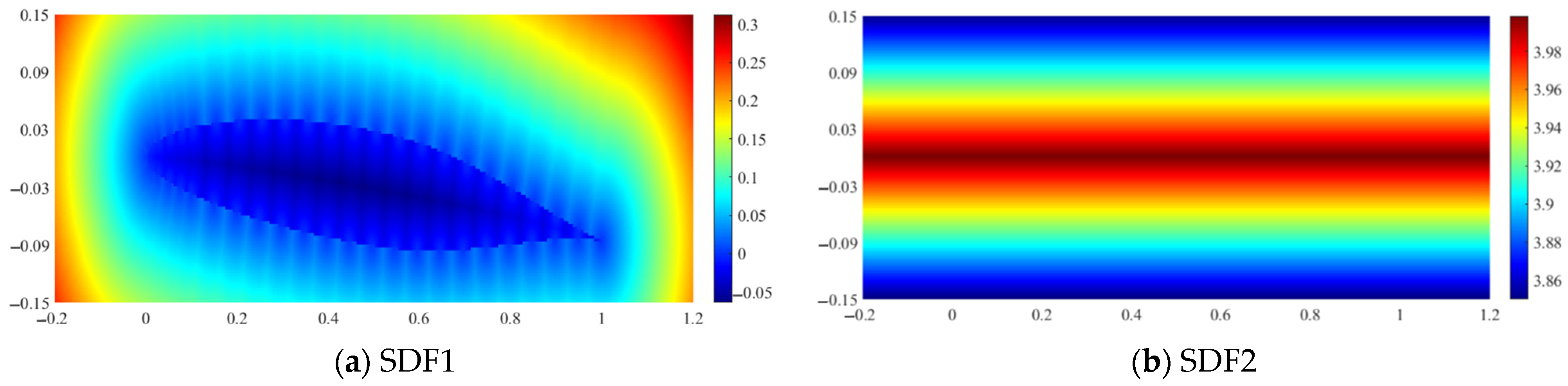
The DeepCFD model utilized the signed distance function (SDF) in two instances: first, to calculate the distance from each point to the surface of the hydrofoil (SDF1), and second, calculate the distance to the top and bottom boundaries (SDF2), as illustrated in Figure 1. To obtain relatively accurate results, the CFD computational domain was configured to a substantial size. However, to minimize the training time of the DeepCFD model, only the data surrounding the hydrofoil were used as inputs for the model.
Figure 1.
SDF1 and SDF2 contours.
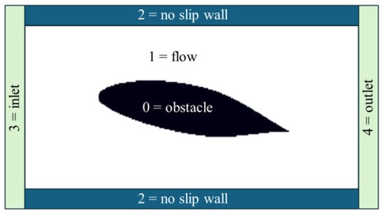
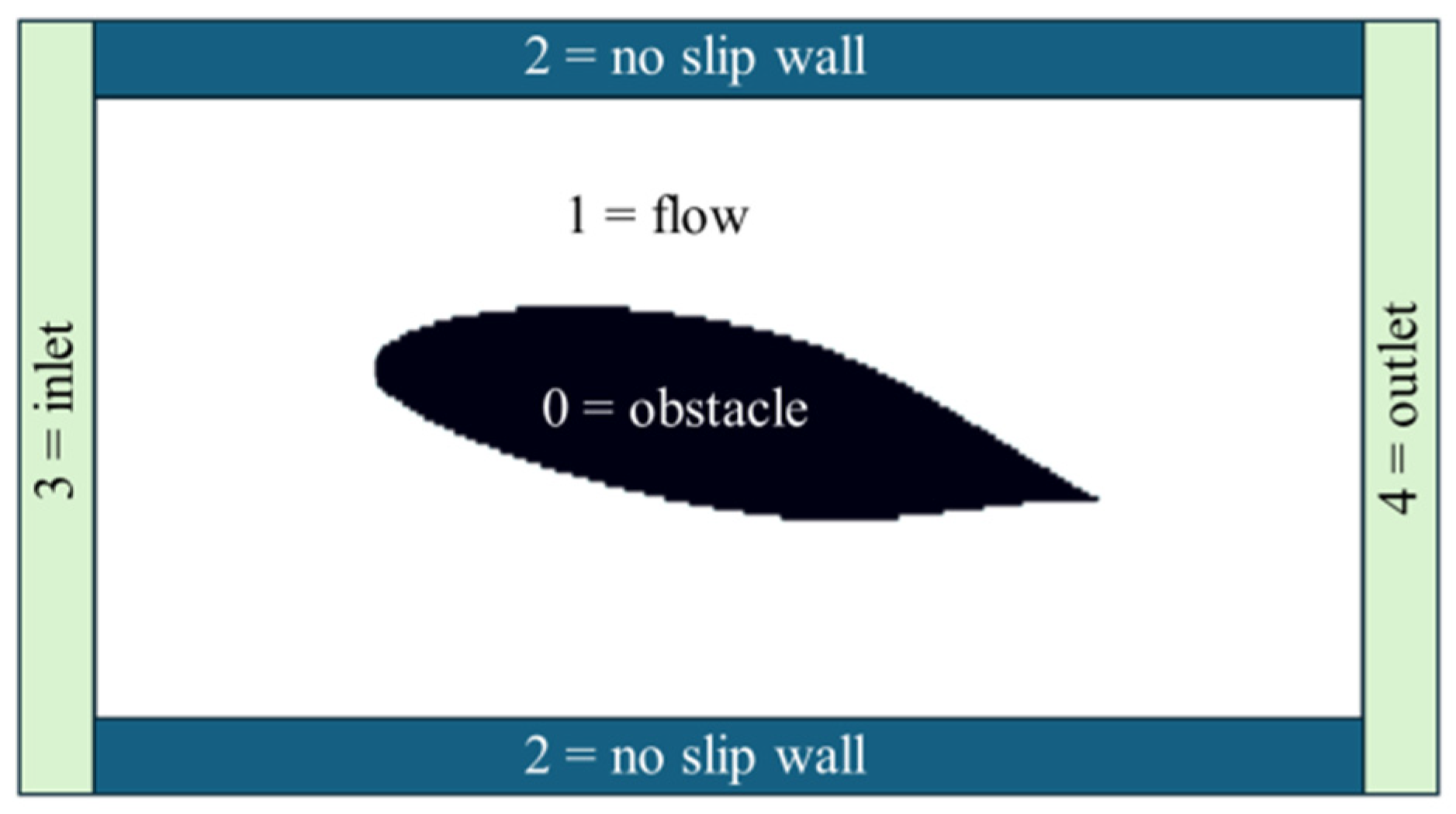
Additionally, a multi-class channel was incorporated to represent the flow region in five distinct categories: 0 for the obstacle, 1 for the free-flow region, 2 for the upper and bottom no-slip wall conditions, 3 for the constant velocity inlet condition, and 4 for the zero-gradient velocity outlet condition, as depicted in Figure 2.
Figure 2.
Input data with multi-class labeling of flow regions.
The components of SDF1, SDF2, and the flow field collectively constitute dataX, while dataY comprises the corresponding computational results, including velocity, pressure, and volume fraction.
3.2. Neural Network Architectures
The DeepCFD model represents an enhancement of the architecture initially proposed by Guo et al. [23]. In the original framework, a downsampling encoder network compresses the geometric information provided by the signed distance function (SDF) into a lower-dimensional latent space, referred to as the latent geometric representation (LGR). This is followed by an upsampling decoder network that reconstructs the LGR back to the data space, with a specific focus on the velocity components. Due to its structural similarity to an autoencoder, this approach is often referred to as an “autoencoder” or simply “AE”. Additionally, each output variable is mapped from the LGR using a separate decoder network.
To enhance the recovery of image details and boundary information while minimizing information loss, the DeepCFD model incorporates a U-Net architecture [27]. The U-Net architecture is characterized by skip connections between corresponding layers of the encoder and decoder, which facilitate the preservation of spatial information and improve the accuracy of the surrogate model in capturing fine details of the flow fields. The symmetric encoder–decoder structure of the U-Net, combined with its skip connections, allows for the simultaneous utilization of both low-level and high-level features. This approach aids in the restoration of detail and edge information, ensuring high-resolution predictions.
The U-Net architecture provides flexibility that allows it to be customized for specific tasks by adjusting parameters such as the number of layers, convolution kernel sizes, and the number of filters. These parameters must be tuned for each particular case study, as outlined in Table 1. In the DeepCFD model, each encoder and decoder block consists of two convolutional layers. The filter configuration in the encoder network is mirrored in reverse order in the decoder network. For instance, if the encoder uses a filter configuration of [8, 16, 32], the decoder will utilize [32, 16, 8]. Max pooling operations are applied at each layer of the encoder to progressively reduce spatial dimensions, while the ReLU activation function introduces non-linearity to the outputs of each layer. Additionally, optional techniques such as batch normalization and weight normalization may be employed to stabilize and accelerate the training process.
Table 1.
Test conditions.
The DeepCFD model employs a 70–30% split of the dataset for training and testing, respectively. The loss function integrates the errors from all three output variables: horizontal velocity (), pressure (), and water phase (). Specifically, the mean squared error (MSE) loss function is applied to the velocity component, while mean absolute error (MAE) is used for both the pressure and water phase outputs. This choice of loss functions was determined through extensive experimentation, which demonstrated that applying the L2-norm (MSE) to the velocity component and the L1-norm (MAE) to the pressure and water phase significantly enhanced the model’s convergence.
4. Model Setting
4.1. Boundary Conditions and Mesh
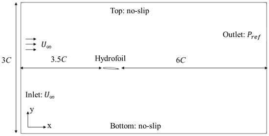
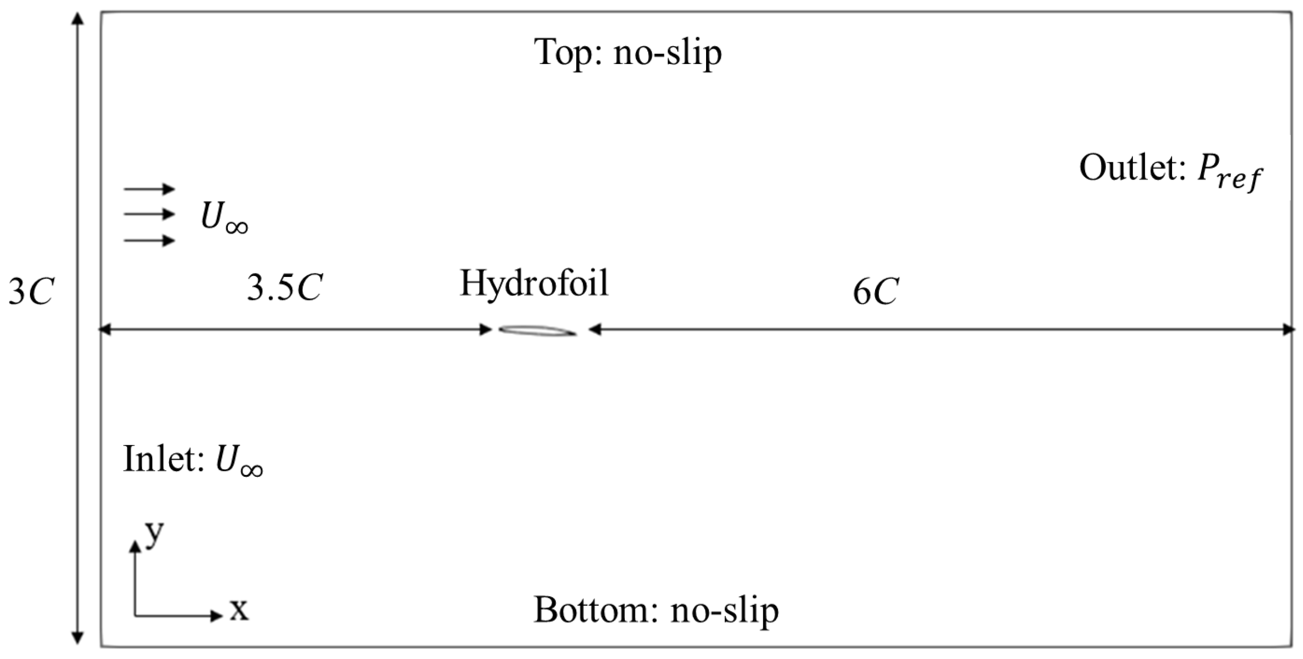
The CFD data used in this study were generated using OpenFOAM 10. The computational domain extends 3.5 times the chord length () upstream of the hydrofoil and 6 times downstream, effectively minimizing the impact of boundary conditions. The total domain length along the flow direction is 10.5 times . Perpendicular to the flow, the inlet boundary length is 3 times . Boundary conditions are consistently maintained across different hydrofoil sections and AoAs. Specifically, a fixed velocity of 2.01 m/s is applied at the inlet (left boundary), a zero-gradient condition for velocity is applied at the outlet (right boundary), and no-slip boundary conditions are enforced on the top, bottom, and hydrofoil surfaces, as illustrated in Figure 3. The velocity was kept constant at 2.01 m/s in order to keep cavitation from changing significantly. The Reynolds stress terms are modeled using the SST k-ω turbulence model, with near-wall treatment applied to the boundary conditions [9].
Figure 3.
Computational domain boundary conditions.
The number of mesh cells varies depending on the hydrofoil, with an average of approximately 42,000 cells. The mesh is refined in the vicinity of the hydrofoil, as depicted in Figure 4. To accurately capture cavitation inception on the hydrofoil, dense meshes in the boundary layer are considered. Table 2 summarizes the grid dependency test. Grid 1 represents the coarsest grid and Grid 4 the finest [28]. The pressure coefficient () is defined as . Here, represents the reference pressure applied at the outlet boundary, and denotes the freestream velocity specified at the inlet boundary. The difference between Grid 3 and Grid 4 is less than 2%, and it can be seen that the impact of the grid on the result is extremely limited at this time. In order to improve the computing efficiency, Grid 3 is selected for simulations.
Figure 4.
Typical computational mesh.
Table 2.
Grid independence summary.
For the time derivative term, a Crank–Nicholson scheme is employed. Convective terms are discretized using the total variation diminishing (TVD) scheme with the van Leer limiter, while diffusive terms are discretized using central differencing. The adjustable time step is applied. The Courant–Friedrichs–Lewy (CFL) number is kept under 0.5 in the simulations.
4.2. Validation
To verify the accuracy of the present simulations for two-dimensional cavitating flows, the study examined cavitating flow around a two-dimensional modified NACA66 hydrofoil at an AoA of four degrees. The hydrofoil exhibited leading-edge cavitation, a phenomenon commonly associated with propeller cavitation. It was observed that cavitation inception could be predicted based on the local pressure. Cavitation occurred when the minimum pressure coefficient, defined as , equaled the cavitation number (σ), which is expressed as
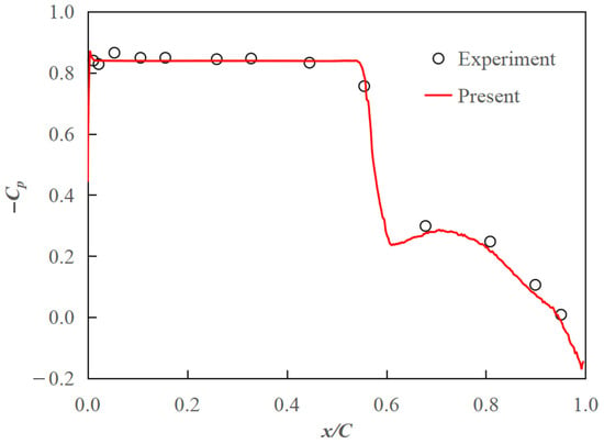
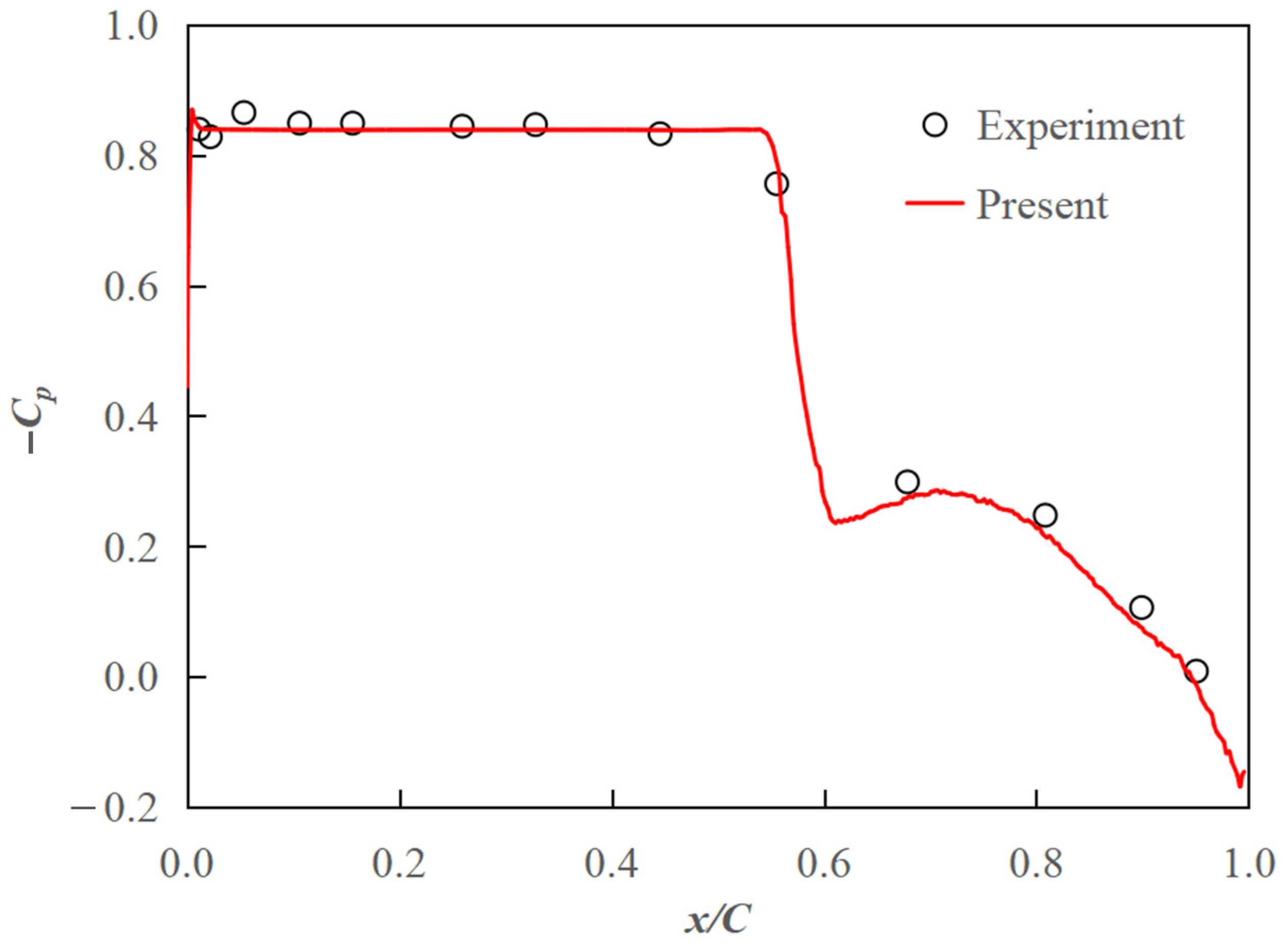
The cavitation characteristics for the hydrofoil section were characterized by the minimum pressure envelope as a function of the cavitation number. Figure 5 displays the pressure coefficient distribution on the surface of the modified NACA66 hydrofoil for a cavitation number of 0.84. Compared to the experimental data from Shen and Dimotakis [29], the present results accurately captured both the cavity closure and the pressure distribution.
Figure 5.
Pressure coefficient distribution on 2D modified NACA66 hydrofoil surface at σ = 0.84.
4.3. Data Processing
To accommodate the need for extensive training data, a total of 400 hydrofoils were considered. This set includes 20 baseline hydrofoils (e.g., NACA 66-021, NACA 64-618, NACA 2412) at an AoA of 0 degrees. The remaining 380 hydrofoils were generated by varying the AoA (0 to 6 degrees) and thickness (−20% to +20%) of the baseline hydrofoils. These variations were created through random transformations in MATLAB. Simulations were conducted to obtain data for 2D cavitating flows around all 400 hydrofoils. The results, including velocity, pressure, and water phase for each hydrofoil, as well as the mesh configuration across the entire computational domain, were recorded and saved.
Since the computational domain in the present simulations is sufficiently large and cavitation typically occurs only near the leading edge of the hydrofoil, only the data in the vicinity of the hydrofoil are required for training. The hydrofoil is fixed at 1 m in length, with its apex at (0, 0). Data were selected from the region spanning −0.13 to 1.13 along the x-axis and −0.15 to 0.15 along the y-axis. This region was divided into a 420 × 170 grid. Due to variations in mesh positions and counts across different hydrofoils, interpolation was necessary to ensure consistent data formatting, as illustrated in Figure 3. The data sampling process was conducted using MATLAB R2022b.
Next, dataX and dataY were converted into NumPy arrays for training the DeepCFD model. The converted arrays have the dimensions (Ns, Nc, Nx, and Ny), where Ns represents the number of samples, Nc denotes the number of channels, and Nx and Ny correspond to the number of elements along the x- and y-directions, respectively. For the input dataX, the first channel contains SDF1 calculated from the hydrofoil surface, the second channel represents the multi-label flow region, and the third channel includes SDF2 calculated from the top and bottom surfaces. For the output dataY file, the first channel corresponds to the horizontal velocity (), the second channel to the pressure (), and the third channel to the water phase (). Each channel comprises 420 (Nx) × 170 (Ny) data points.
5. Results and Discussion
5.1. Prediction for Different Cavity Patterns
Predictions were performed using DeepCFD for various cavity patterns. The same numerical method was applied across all CFD computations, and results from the same time step ( = 12 s) were compared, as cavitation patterns evolve over time. The cavitation constants, and , were set to 0.2 for both model training and prediction.
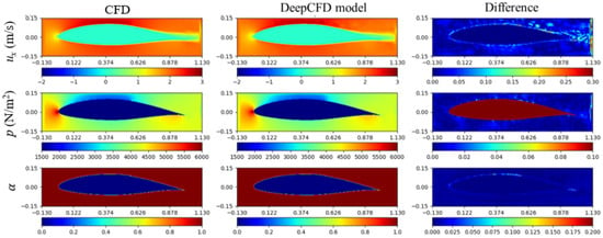
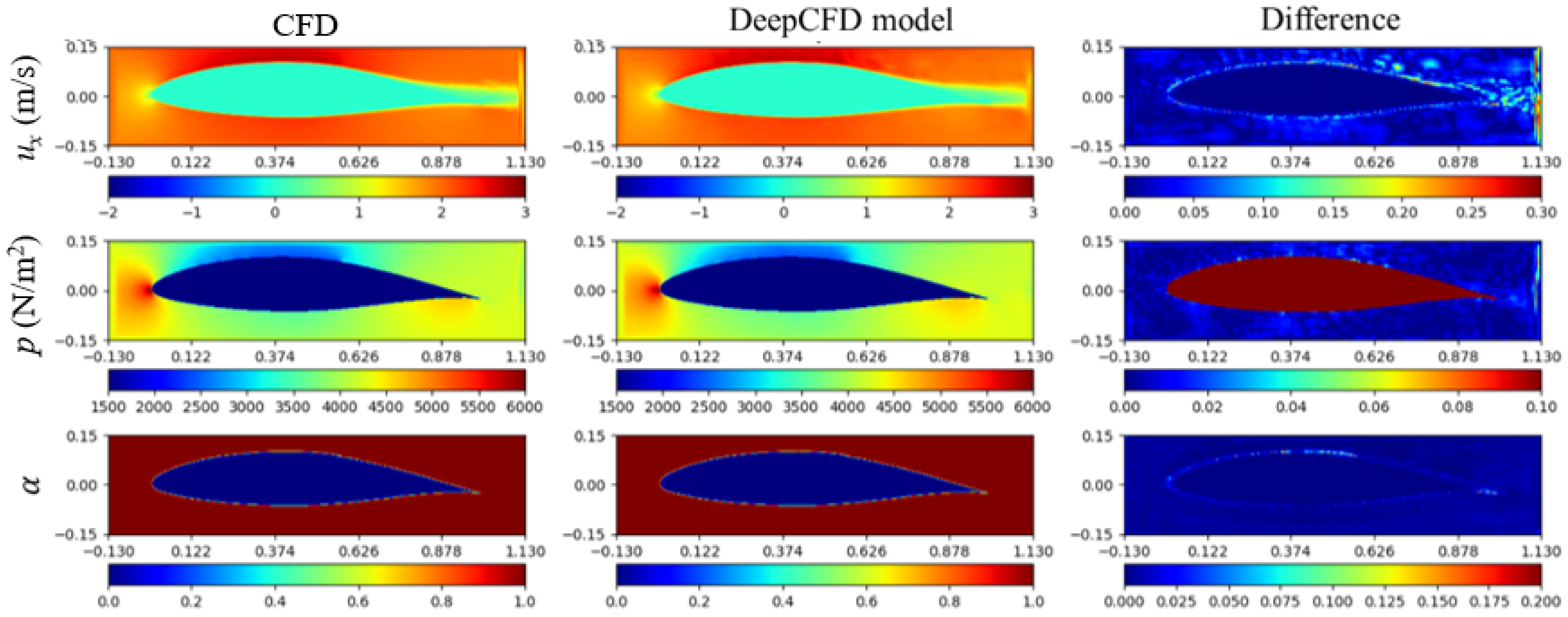
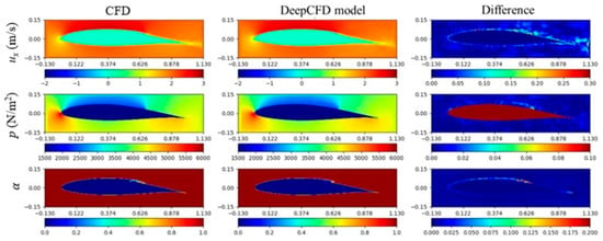
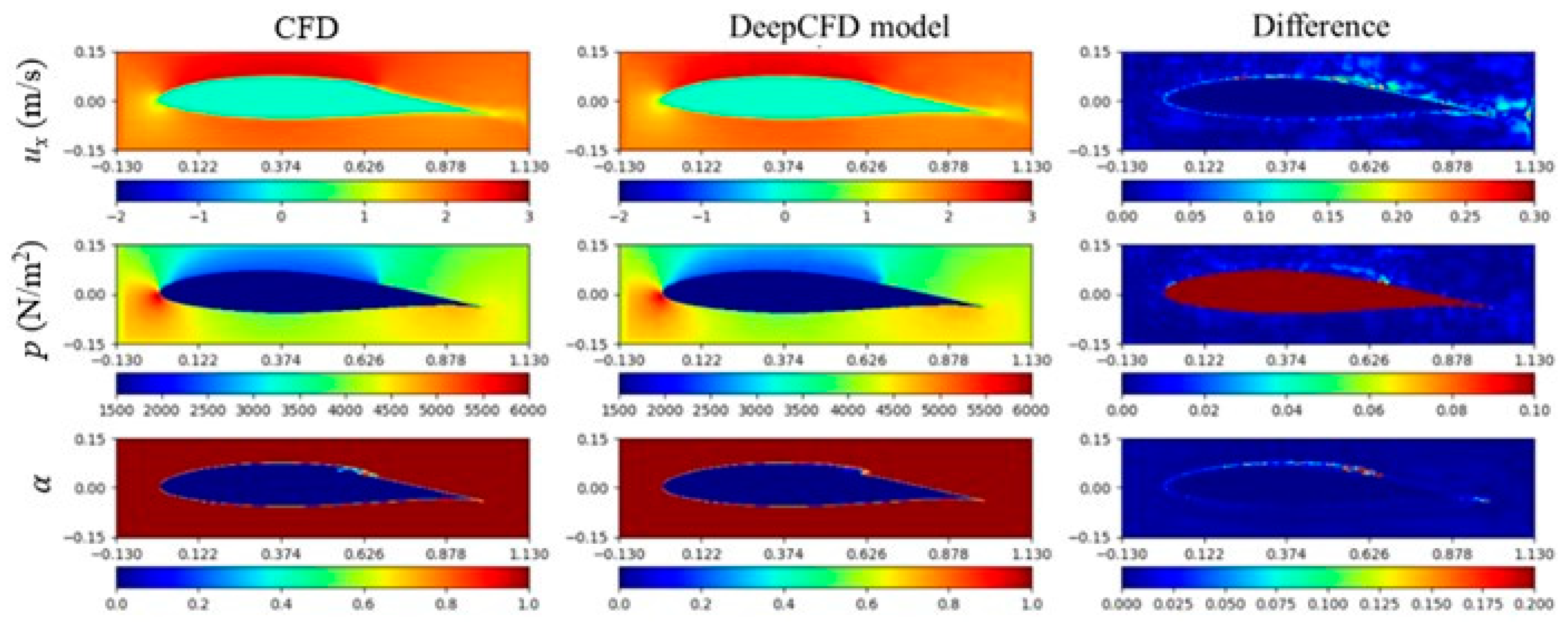
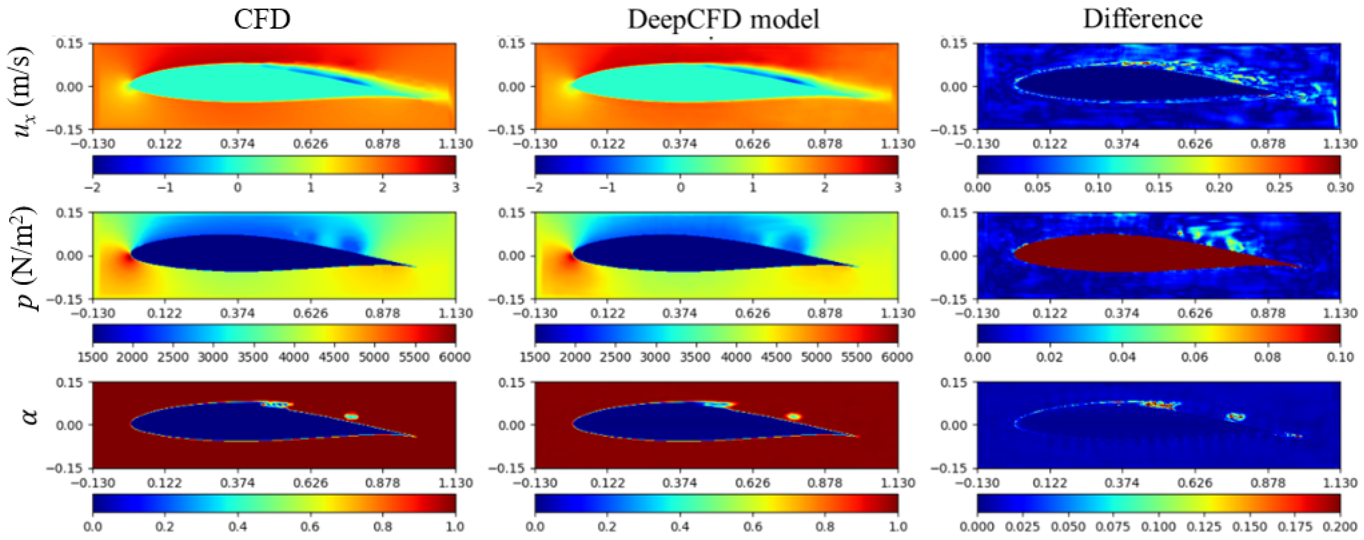
First, a non-cavitating flow scenario (the 245th test sample) was considered. Figure 6 presents the results for this case, where no cavitation was observed on the hydrofoil at that time. The figure is organized as follows: the first column displays the CFD results, the second column shows the DeepCFD predictions, and the third column illustrates the difference between the CFD results and the DeepCFD predictions. For the horizontal velocity (m/s) and the water phase (), the absolute differences () and () are shown due to the relatively small magnitude of these quantities. Conversely, for pressure p(), the relative difference (( is presented, as pressure values are larger and change more rapidly near cavitation regions. As depicted in Figure 6, for non-cavitating flow, the DeepCFD model accurately predicts the relevant flow characteristics around the hydrofoil, resulting in minimal differences.
Figure 6.
Non-cavitating flow (245th test sample) by present CFD and DeepCFD model ( = 12 s).
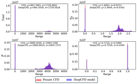
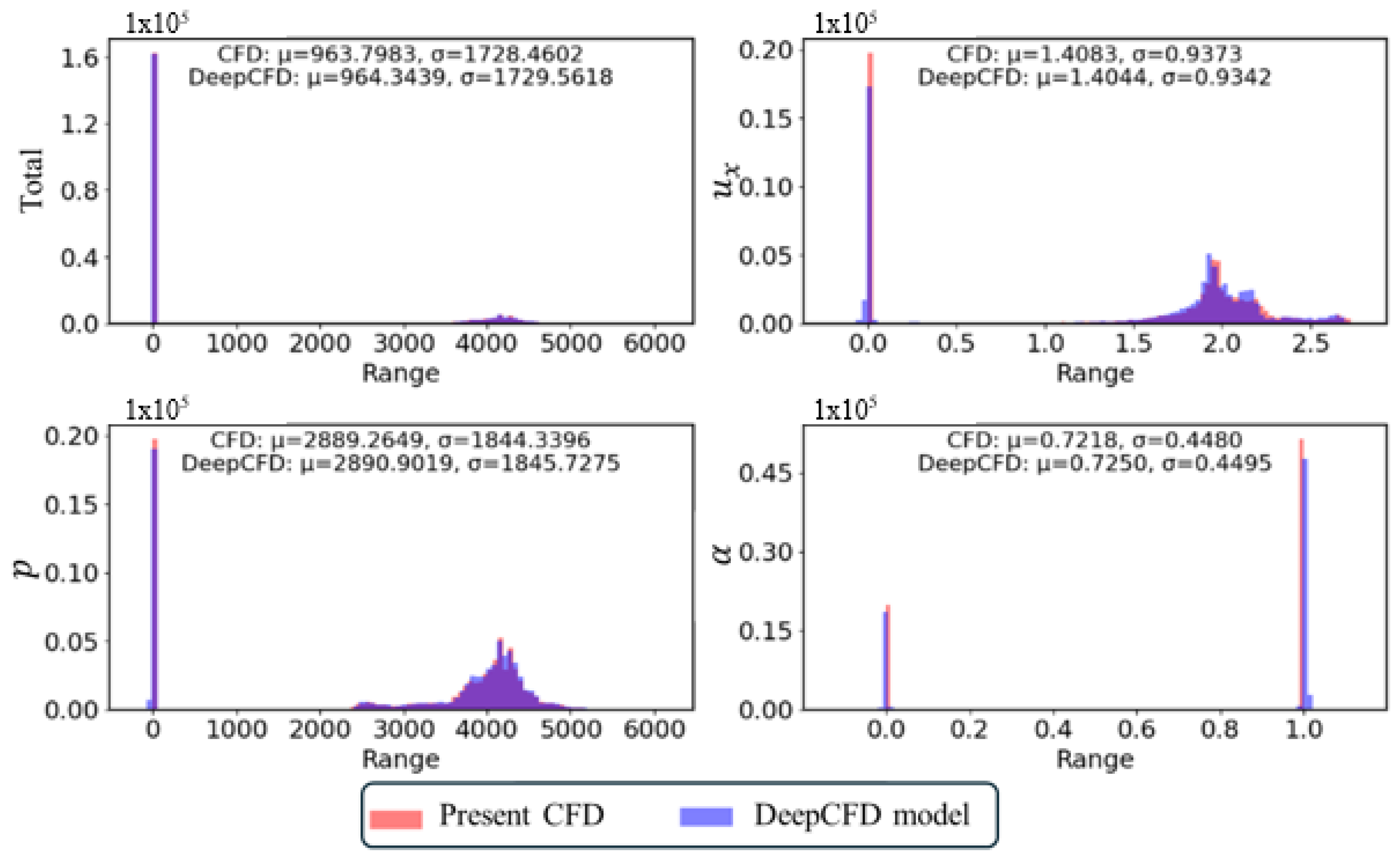
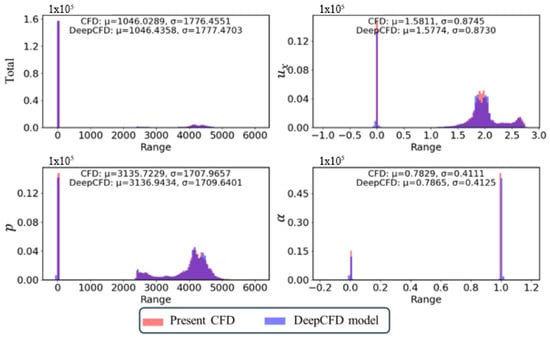
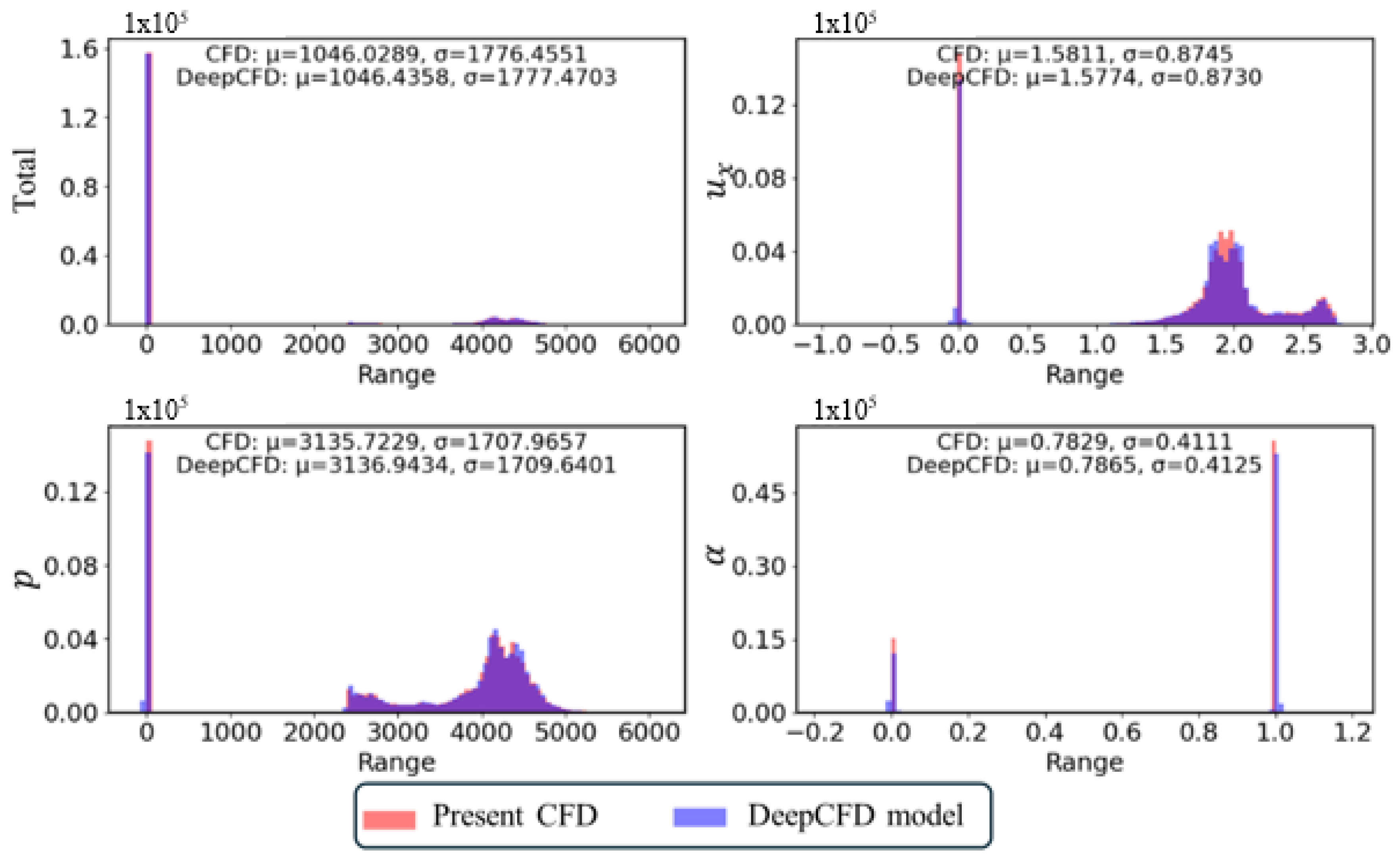
Figure 7 compares the data distributions for the non-cavitating flow (the 245th test sample) obtained from the present CFD simulations and the DeepCFD model. The top left image shows the combined data for all variables (, p, and ), while the other images depict the data distribution for each specific variable. Consistent with the qualitative results previously presented, the data distributions generated by the DeepCFD model closely match those from the CFD simulations. Furthermore, the differences in mean values () and standard deviations () between the two methods are minimal, less than , demonstrating a strong agreement between the DeepCFD predictions and the CFD results.
Figure 7.
Data distribution (245th test sample) for non-cavitating flow by present CFD and DeepCFD model ( = 12 s).
The sheet cavitating flow scenario (150th test sample) was analyzed. Figure 8 presents the results for this case, where sheet cavitation was observed on the hydrofoil at = 12 s. Although the sheet cavitation appears steady, the flow at the end of the cavity becomes unsteady due to the presence of re-entrant jets. The differences highlighted in the figure are primarily concentrated around the cavity closure. The region near the cavity end involves complex physical phenomena, including rapid and uneven changes in scale, which makes accurately capturing the interface challenging. The present CFD simulations also exhibit some discrepancies near the cavity end. However, these differences are deemed acceptable given the inherent difficulties in precisely capturing these intricate regions.
Figure 8.
Sheet cavitating flow (150th test sample) by present CFD and DeepCFD model ( = 12 s).
Figure 9 illustrates the data distribution for the sheet cavitating flow (the 150th test sample) as predicted by both the present CFD simulations and the DeepCFD model. The distribution shapes notably differ from those observed in non-cavitating flow scenarios. Despite these differences, the data distributions produced by both methods remain similar in shape, with only minor discrepancies in mean values and standard deviations. Even with the variations introduced by cavitation, the DeepCFD model continues to closely align with the results obtained from the CFD simulations.
Figure 9.
Data distribution (150th test sample) for sheet cavitating flow by present CFD and DeepCFD model ( = 12 s).
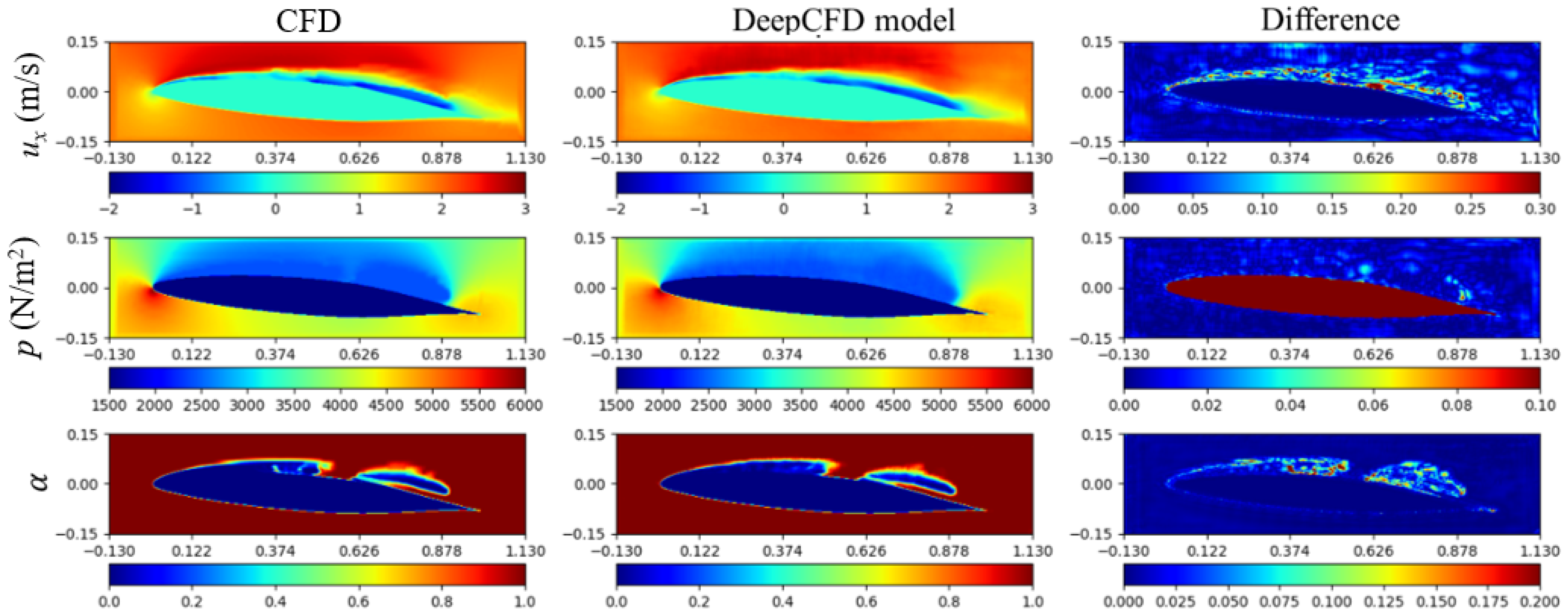
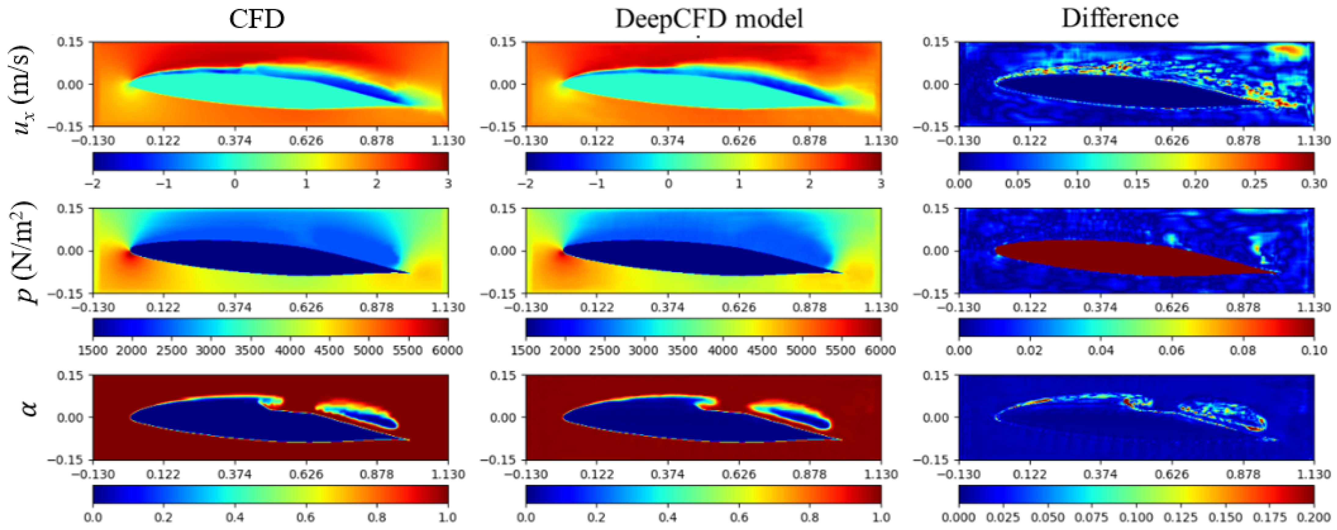
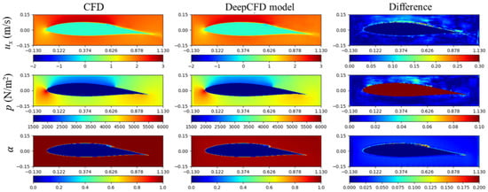
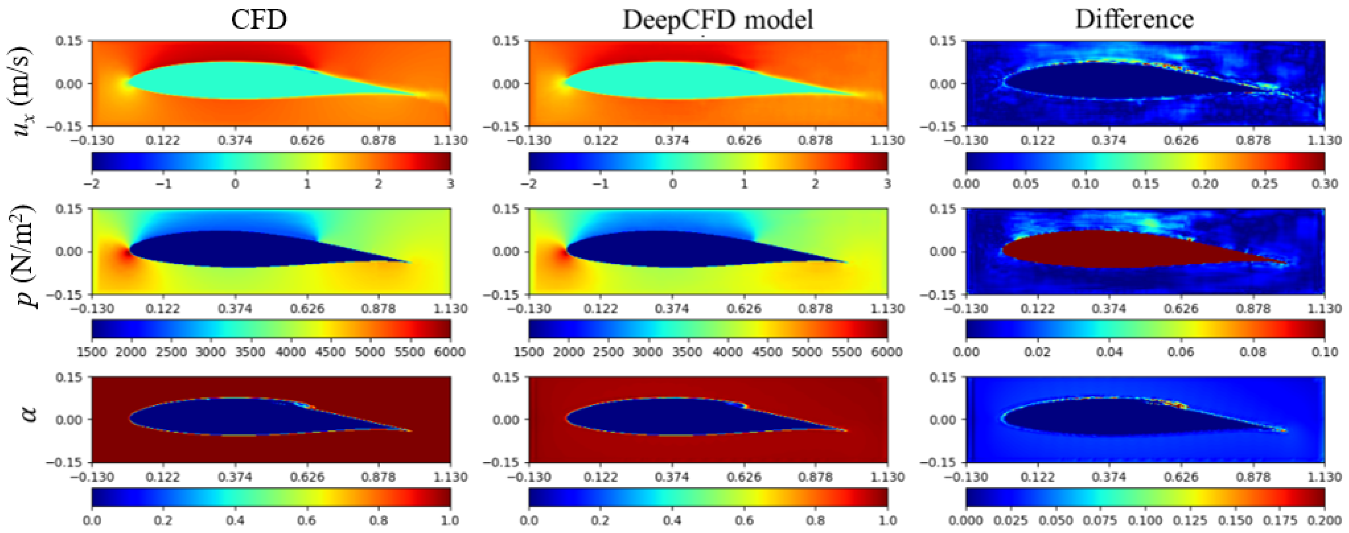
The detached cavitating flow scenario (the 120th test sample) was examined. Figure 10 presents the results for this case, where detached cavitation was observed on the hydrofoil at = 12 s. Unlike the non-cavitating and sheet cavitating flows, there are noticeable differences in the predictions for horizontal velocity and water phase. However, the predictions for pressure exhibit a high degree of consistency with the present CFD results, with only minor discrepancies observed at the leading and trailing edges of the detached cavity.
Figure 10.
Detached cavitating flow (120th test sample) by present CFD and DeepCFD model ( = 12 s).
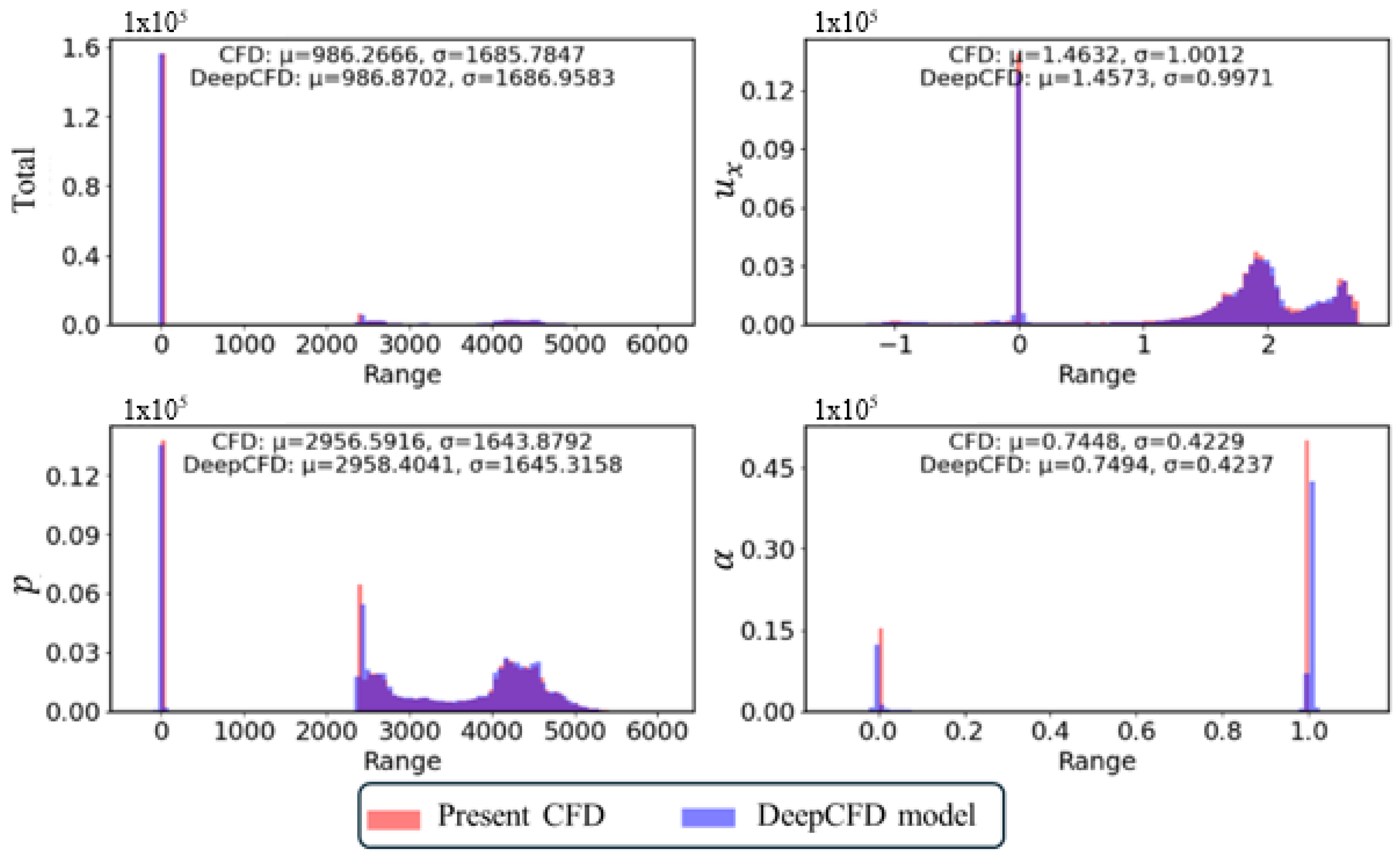
Figure 11 compares the data distribution for the detached cavitating flow (the 120th test sample) obtained from both the present CFD simulations and the DeepCFD model. Consistent with previous comparisons, the results from both methods exhibit minimal differences. The data distributions align closely, demonstrating that the DeepCFD model maintains a high level of accuracy even in more complex cavitation scenarios.
Figure 11.
Data distribution (150th test sample) for detached cavitating flow by present CFD and DeepCFD model ( = 12 s).
Given the large number of cases, it is impractical to display each one individually. However, the analysis of the three cavity patterns presented demonstrates that the DeepCFD model effectively predicts cavitation around various hydrofoils, including sheet cavitation. Although some discrepancies are observed in the predictions for detached cavitation, the model’s predictions for pressure remain particularly accurate.
5.2. Prediction for Transient Cavity
As previously noted, detached cavitation induces continuous fluctuations in the flow around the hydrofoil. To investigate the transient behavior of the cavity, results at = 30 s were selected. This timeframe allows for an examination of how varying the simulation duration influences the accuracy of the model’s predictions.
Figure 12 displays the results for the 150th test sample, where cavitation was observed on the hydrofoil at = 30 s. At this later time, the sheet cavitation previously observed at = 12 s has moved downstream. The predictions by the DeepCFD model remain consistent with those from = 12 s, showing minor differences in horizontal velocity and water phase around the cavity end, while the difference in pressure remains notably smaller. Overall, despite changes in simulation time, the DeepCFD model continues to deliver accurate predictions of cavitation.
Figure 12.
Cavitating flow (150th test sample) by present CFD and DeepCFD model ( = 30 s).
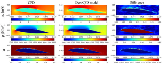
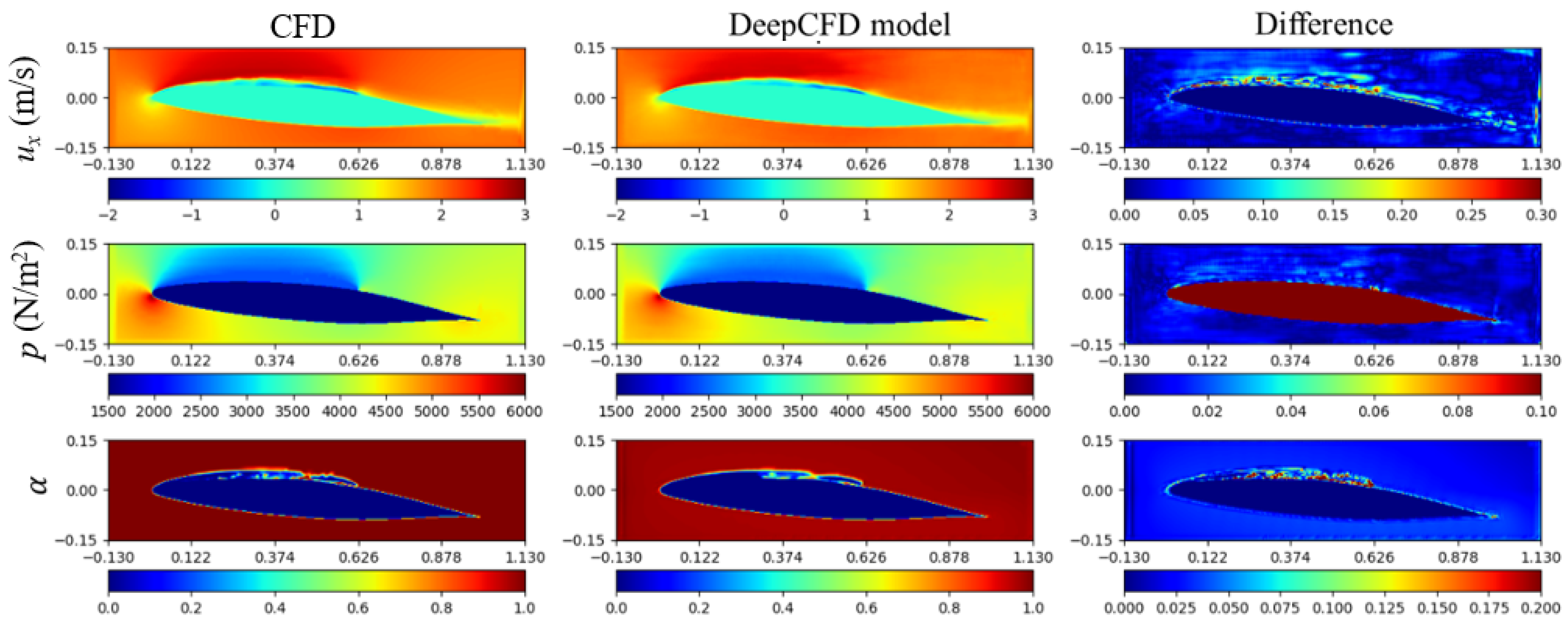
Figure 13 illustrates the results for the 120th test sample, where detached cavitation was observed on the hydrofoil at = 30 s. For the detached cavitation scenario, the differences in predictions between = 12 and = 30 s were similar. Notably, some discrepancies were observed in the horizontal velocities, while only minor differences were seen in the water phase contours, particularly around the cavity interfaces.
Figure 13.
Cavitating flow (120th test sample) by present CFD and DeepCFD model ( = 30 s).
5.3. Prediction with Different Cavitation Model Constants
The cavitation model constants ( and ) are crucial parameters in cavitation simulations, and their adjustment can significantly impact the accuracy of the results. To explore their effects, different values for these constants, specifically = = 1, were considered, with the simulation time maintained at = 12 s.
The sheet cavitating flow (the 150th test sample) was examined with = . Figure 14 presents the results for this case, where sheet cavitation was observed on the hydrofoil at = 12 s. Although the cavity length remains consistent across different model constants, differences are noted due to the presence of the re-entrant jet. Despite varying the model constants, the discrepancies in horizontal velocity, pressure, and water phase are quite similar to those observed with = .
Figure 14.
Sheet cavitating flow (150th test sample) by present CFD and DeepCFD model with = ( = 12 s).
The detached cavitating flow scenario (120th test sample) was analyzed with = . Figure 15 illustrates the results for this case, where detached cavitation was observed on the hydrofoil at = 12 s. With these model constants, the shape of the detached cavity became more complex. Notable differences were observed in the horizontal velocity. However, discrepancies in the water phase were confined to the cavity interface, with the overall shape and length of the cavity remaining well predicted. Thus, varying the model constants does not significantly impact the accuracy of the DeepCFD model.
Figure 15.
Detached cavitating flow (120th test sample) by present CFD and DeepCFD model with = ( = 12 s).
6. Concluding Remarks
Traditional CFD methods for cavitation predictions are accurate but often computationally intensive, requiring significant time and resources. To address these challenges, there is increasing interest in applying deep learning approaches to CFD modeling. In this study, the DeepCFD model was employed to predict cavitation around hydrofoils. DeepCFD is a deep learning-based CFD methodology that leverages deep neural networks to substantially reduce computational time while maintaining a reasonable level of accuracy.
DeepCFD requires a substantial amount of high-quality training data. To generate these data, OpenFOAM, an open-source CFD library, was utilized for cavitation simulations. Initially, 20 baseline hydrofoils were selected, and 380 additional hydrofoils were created by varying the angle of attack (AoA) and thickness using MATLAB’s random functions. After simulating a total of 400 different cases, the results for velocity components, pressure, and water phase were used to train the DeepCFD model. The DeepCFD model employs a U-Net architecture, which involves numerous parameters that needed to be carefully configured. The specific parameter settings for the relevant cases were detailed accordingly.
The DeepCFD model was employed to predict various cavitation scenarios, including non-cavitating, sheet cavitating, and detached cavitating flows. These predictions were compared with results from the current CFD simulations. For non-cavitating flow, the DeepCFD model delivered accurate predictions for both velocity and pressure. In sheet cavitating flow scenarios, the model generally performed well, although some discrepancies were noted due to the transient behavior of re-entrant jets near the cavity end. For detached cavitation, while there were minor inaccuracies in velocity predictions, the model effectively predicted the cavity’s length and shape. Overall, variations in model constants had a minimal impact on the accuracy of the DeepCFD predictions.
Comparisons between CFD results and DeepCFD predictions showed that the DeepCFD model maintained high accuracy in predicting cavitation phenomena. Compared with the numerical simulation results, the difference between the mean and standard deviation is less than 3 ‰. Even with variations in simulation time or adjustments to the cavitation model constants CC and CV, the model demonstrated robustness. Minor discrepancies were observed primarily at the edges of cavitation bubbles, highlighting that the DeepCFD model remains reliable and consistent across different simulation parameters. Comparing the computational time, for a typical two-dimensional cavitation, with 20 cores, the results are sufficient in 30 min. However, with the DeepCFD model, it takes no more than 10 s. Therefore, using the DeepCFD model can significantly reduce the computational cost.
For future work, the current two-dimensional approach will be extended to three-dimensional flow configurations to capture more intricate cavitation phenomena. Additionally, efforts will be undertaken to broaden the dataset, thereby enhancing the model’s generalizability and accuracy across a more diverse set of conditions and hydrofoil geometries. This will facilitate its use in real-world applications, such as optimizing the design of marine vessels for improved efficiency and reduced cavitation-induced damage, and in the predictive maintenance of existing naval architectures.
Author Contributions
Conceptualization, B.L. and S.P.; methodology, B.L. and S.P.; validation B.L. and S.P.; simulation, B.L.; formal analysis, B.L.; writing—original draft preparation, B.L.; writing—review and editing, B.L. and S.P.; visualization, B.L.; supervision S.P.; funding acquisition, S.P. All authors have read and agreed to the published version of the manuscript.
Funding
This research was supported by the National Research Foundation of Korea (NRF-2021R1I1A3044639).
Institutional Review Board Statement
Not applicable.
Informed Consent Statement
Not applicable.
Data Availability Statement
The original contributions presented in the study are included in the article, further inquiries can be directed to the corresponding author.
Conflicts of Interest
The authors declare no conflicts of interest.
Nomenclature
| Symbols | |||
| Velocity | Experimental constant | ||
| Pressure | Experimental constant | ||
| Saturated pressure | Source term | ||
| Reference pressure | Subset of a metric space | ||
| Freestream velocity | Blending function | ||
| Kinetic energy | Blending function | ||
| Dissipation rate | Initial nucleus diameter | ||
| Greek | |||
| Volume fraction | Density | ||
| Eddy viscosity | Nucleation fraction | ||
| CC | Condensation coefficients | CV | Evaporation coefficients |
| σ | Cavitation number | ||
| Subscripts | |||
| i | x directions | j | y directions |
| k | z directions | ||
References
- Callenaere, M.; Franc, J.-P.; Michel, J.-M.; Riondet, M. The cavitation instability induced by the development of a re-entrant jet. J. Fluid Mech. 2001, 444, 223–256. [Google Scholar] [CrossRef] [Scilit]
- Huang, B.; Wang, G. Experimental and numerical investigation of unsteady cavitating flows through a 2D hydrofoil. Sci. China Technol. Sci. 2011, 54, 1801–1812. [Google Scholar] [CrossRef] [Scilit]
- Long, Y.; Long, X.; Ji, B.; Xing, T. Verification and validation of Large Eddy Simulation of attached cavitating flow around a Clark-Y hydrofoil. Int. J. Multiph. Flow 2019, 115, 93–107. [Google Scholar] [CrossRef] [Scilit]
- Lin, C.; Zhao, X.; Wang, Z.; Cheng, H.; Wang, C.; Ji, B. Large eddy simulations of sheet-to-cloud cavitation transitions with special emphasis on the simultaneous existence of the re-entrant jet and shock waves. J. Turbul. 2024, 25, 157–180. [Google Scholar] [CrossRef] [Scilit]
- Park, S.; Yeo, H.; Hyung Rhee, S. Isothermal compressible flow solver for prediction of cavitation erosion. Eng. Appl. Comput. Fluid Mech. 2019, 13, 683–697. [Google Scholar] [CrossRef] [Scilit]
- Gaggero, S.; Tani, G.; Viviani, M.; Conti, F. A study on the numerical prediction of propellers cavitating tip vortex. Ocean Eng. 2014, 92, 137–161. [Google Scholar] [CrossRef] [Scilit]
- Yilmaz, N.; Atlar, M.; Khorasanchi, M. An improved Mesh Adaption and Refinement approach to Cavitation Simulation (MARCS) of propellers. Ocean Eng. 2019, 171, 139–150. [Google Scholar] [CrossRef] [Scilit]
- Viitanen, V.; Siikonen, T.; Sánchez-Caja, A. Cavitation on model-And full-scale marine propellers: Steady and transient viscous flow simulations at different Reynolds numbers. J. Mar. Sci. Eng. 2020, 8, 141. [Google Scholar] [CrossRef] [Scilit]
- Ng’aru, J.M.; Park, S. Computational Analysis of Cavitating Flows around a Marine Propeller Using Incompressible, Isothermal Compressible, and Fully Compressible Flow Solvers. J. Mar. Sci. Eng. 2023, 11, 2199. [Google Scholar] [CrossRef] [Scilit]
- Shankar, V.; Portwood, G.D.; Mohan, A.T.; Mitra, P.P.; Krishnamurthy, D.; Rackauckas, C.; Wilson, L.A.; Schmidt, D.P.; Viswanathan, V. Validation and parameterization of a novel physics-constrained neural dynamics model applied to turbulent fluid flow. Phys. Fluids 2022, 34, 115110. [Google Scholar] [CrossRef] [Scilit]
- Kwon, B.; Ejaz, F.; Hwang, L.K. Machine learning for heat transfer correlations. Int. Commun. Heat Mass Transf. 2020, 116, 104694. [Google Scholar] [CrossRef] [Scilit]
- Fonda, E.; Pandey, A.; Schumacher, J.; Sreenivasan, K.R. Deep learning in turbulent convection networks. Proc. Natl. Acad. Sci. USA 2019, 116, 8667–8672. [Google Scholar] [CrossRef] [Scilit] [PubMed]
- Fukami, K.; Fukagata, K.; Taira, K. Assessment of supervised machine learning methods for fluid flows. Theor. Comput. Fluid Dyn. 2020, 34, 497–519. [Google Scholar] [CrossRef] [Scilit]
- Ling, J.; Kurzawski, A.; Templeton, J. Reynolds averaged turbulence modelling using deep neural networks with embedded invariance. J. Fluid Mech. 2016, 807, 155–166. [Google Scholar] [CrossRef] [Scilit]
- Lui, H.F.S.; Wolf, W.R. Construction of reduced-order models for fluid flows using deep feedforward neural networks. J. Fluid Mech. 2019, 872, 963–994. [Google Scholar] [CrossRef] [Scilit]
- Jeon, W.; Park, S.; Cho, S.-k. Moored motion prediction of a semi-submersible offshore platform in waves using an OpenFOAM and MoorDyn coupled solver. Int. J. Nav. Archit. Ocean Eng. 2023, 15, 100544. [Google Scholar] [CrossRef] [Scilit]
- Asnaghi, A.; Petit, O.; Lackmann, T. CFD with OpenSource Software. 2013. Available online: https://www.tfd.chalmers.se/~hani/kurser/OS_CFD_2013/AbolfazlAsnagi/interPhasChangeFoam_and_PANSTurbulenceModel.pdf (accessed on 21 June 2024).
- Hirt, C.W.; Nichols, B.D. Volume of fluid (VOF) method for the dynamics of free boundaries. J. Comput. Phys. 1981, 39, 201–225. [Google Scholar] [CrossRef] [Scilit]
- Wilcox, D.C. Turbulence Modeling for CFD (Hardcover), 3rd ed.; Dcw Industries: La Canada, CA, USA, 2006. [Google Scholar]
- Ghafoorian, F.; Mirmotahari, S.R.; Wan, H. Numerical study on aerodynamic performance improvement and efficiency enhancement of the savonius vertical axis wind turbine with semi-directional airfoil guide vane. Ocean Eng. 2024, 307, 118186. [Google Scholar] [CrossRef] [Scilit]
- Huang, H.; Sun, T.; Zhang, G.; Li, D.; Wei, H. Evaluation of a developed SST k-ω turbulence model for the prediction of turbulent slot jet impingement heat transfer. Int. J. Heat Mass Transf. 2019, 139, 700–712. [Google Scholar] [CrossRef] [Scilit]
- Schnerr, G.H.; Sauer, J. Physical and numerical modeling of unsteady cavitation dynamics. In Proceedings of the Fourth International Conference on Multiphase Flow, New Orleans, LA, USA, 27 May–1 June 2001; pp. 1–12. [Google Scholar]
- Guo, X.; Li, W.; Iorio, F. Convolutional Neural Networks for Steady Flow Approximation. In Proceedings of the 22nd ACM SIGKDD International Conference on Knowledge Discovery and Data Mining, San Francisco, CA, USA, 13–17 August 2016; pp. 481–490. [Google Scholar]
- Ribeiro, M.D.; Rehman, A.; Ahmed, S.; Dengel, A. DeepCFD: Efficient steady-state laminar flow approximation with deep convolutional neural networks. arXiv 2020, arXiv:2004.08826. [Google Scholar]
- Afzal, M.Z.; Capobianco, S.; Malik, M.I.; Marinai, S.; Breuel, T.M.; Dengel, A.; Liwicki, M. Deepdocclassifier: Document classification with deep Convolutional Neural Network. In Proceedings of the 2015 13th International Conference on Document Analysis and Recognition (ICDAR), Tunis, Tunisia, 23–26 August 2015; pp. 1111–1115. [Google Scholar]
- Sekar, V.; Zhang, M.; Shu, C.; Khoo, B.C. Inverse Design of Airfoil Using a Deep Convolutional Neural Network. AIAA J. 2019, 57, 993–1003. [Google Scholar] [CrossRef] [Scilit]
- Ronneberger, O.; Fischer, P.; Brox, T. U-net: Convolutional networks for biomedical image segmentation. In Proceedings of the Medical Image Computing and Computer-Assisted Intervention–MICCAI 2015: 18th International Conference, Munich, Germany, 5–9 October 2015; pp. 234–241. [Google Scholar]
- Ghafoorian, F.; Mirmotahari, S.R.; Eydizadeh, M.; Mehrpooya, M. A systematic investigation on the hybrid Darrieus-Savonius vertical axis wind turbine aerodynamic performance and self-starting capability improvement by installing a curtain. Next Energy 2025, 6, 100203. [Google Scholar] [CrossRef] [Scilit]
- Shen, Y.; Dimotakis, P. The influence of Surface Cavitation on Hydrodynamic Forces. In Proceedings of the SNAME 22nd American Towing Tank Conference, St. John’s, NF, Canada, 8–11 August 1989. [Google Scholar]



Disclaimer/Publisher’s Note: The statements, opinions and data contained in all publications are solely those of the individual author(s) and contributor(s) and not of MDPI and/or the editor(s). MDPI and/or the editor(s) disclaim responsibility for any injury to people or property resulting from any ideas, methods, instructions or products referred to in the content. |
© 2024 by the authors. Licensee MDPI, Basel, Switzerland. This article is an open access article distributed under the terms and conditions of the Creative Commons Attribution (CC BY) license (https://creativecommons.org/licenses/by/4.0/).