


Abstract
There are many methods for crushing seabed rock such as a using a free-falling crusher, blasting, and chemical liquid expansion. Blasting and chemical liquid expansion can lead to environmental destruction, noise pollution, and civil complaints. Therefore, a free-falling crusher is generally recommended for use. Understanding the characteristics of a crusher in water and the impact force on the ground is helpful for designing a crusher and dredge work. In this study, drop tests of 50 and 70 ton crusher models that were scaled down by 15 times were investigated. The tests were conducted in a water basin by the Research Institute of Medium and Small Shipbuilding (RIMS) in Korea. Four water depths were considered with different falling locations: water surface and air. Moreover, a numerical study on Fluid-Structure Interaction (FSI) analysis for a free-falling crusher was conducted by applying the Arbitrary Lagrangian-Eulerian (ALE) element and the Grüneisen Equation of State (EoS) to fluid models. The crusher and ground were modeled as Lagrangian elements to estimate the impact force on the ground. Before comparing the crusher model, a free-falling sphere model was used to develop FSI technologies by comparing past Computational Fluid Dynamics (CFD) and experimental results. Moreover, the recommended mesh size and fluid domain for FSI analysis are provided to achieve good results via convergence tests. Comparison between experimental and numerical methods demonstrated a similar tendency such that impact force increased at a higher depth. Certain numerical results agree with average values of experimental results; however, multiple numerical cases exhibit a moderate difference. This is because of angular rotation between the crusher and ground when the crusher hits the ground during experiments.
1. Introduction
Currently, there are multiple types of dredging methods available for use: Pump-type, which inhales soil using a pump; and grab-type, which uses a grab bucket [1]. However, these methods can be ineffective when rock removal is necessary. To crush underwater rock, the blasting method and a method that expands rock by adding chemical fluid are commonly used; however, these methods can cause damage to surrounding structures and result in civil complaints because of noise or environmental pollution [2,3]. A crusher is recommended when blasting and expansion methods are not suitable. There are two types of crushers depending on how seabed rocks are broken apart: a central-type crusher uses the impact force generated by the free-falling of the crusher at an appropriate height and an impact-type crusher repeatedly hits rock with compressed air. The free-falling crusher is easier to use and is less expensive. Previously, studies have been conducted on crushers used for removing rocks. The performance of the impact crusher was determined by the rotor radius, angular velocity, feed rate, and feed size distribution functions was tested by Nikolov et al. [4]. Cleary et al. examined the performance of a cone-type crusher based on crusher material characteristics and operating conditions [5]. However, most studies have focused on crushers that were used on land. In this study, a crusher that operates in water is analyzed.
It is important to estimate the capabilities of a crusher in the early stage of design to determine crusher size and strength. The best approach to verify crusher performance is the experimental approach; however, experiments have several limitations such as space, cost, and time restrictions. A numerical simulation approach is an alternative approach to confirm the crusher behavior. Fluid-Structure Interaction (FSI) analysis has an advantage when it is used to contemplate the effect of a surrounding fluid on a structure because it accounts for the interrelation effect between fluids and structures. Especially, underwater collision studies have been actively undertaken through FSI analysis in marine research areas. Kim et al. [6] emphasized on considering multi-physics simulations for collision or grounding events because of the influence of hydrodynamic restoring forces. Lee et al. [7] used FSI to determine the extent of damage to a transport vessel and container under collision and stranding. Furthermore, Song et al. [8] examined the effect of forwarding velocity and mass of a struck ship and the impact angle on ship collisions using FSI analysis.
Table 1 highlights the several research for dropping an object using different methods. Most studies were performed based on Computational Fluid Dynamics (CFD) analysis to evaluate the underwater behavior of an object. However, it is not able to assess the structural response of the ground when an object hits the ground. For evaluating structural response, such as impact force, FSI analysis is an alternative method by considering water resistance, which is an important factor that decreases impact force. Therefore, the surrounding fluid has to be included in the entire numerical analysis while the object moves into the water. For this purpose, it is important to develop numerical techniques by confirming their results with experiments. However, only a simple sphere structure was tested experimentally. A scaled-down crusher model was developed and an impact force test was performed to assess crusher performance.
Table 1.
Various studies on dropping object.
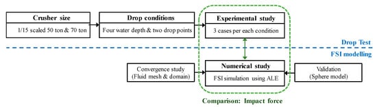
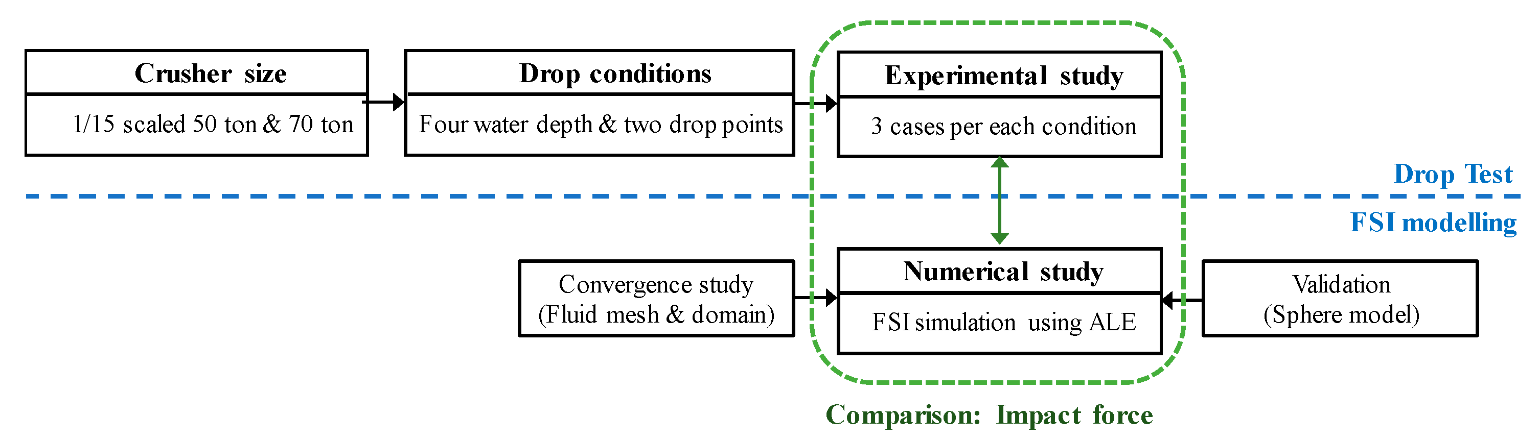
Figure 1 represents two main steps of this study. Tests for dropping the crusher in the water were performed in a water basin by the Research Institute of Medium and Small Shipbuilding (RIMS) in Korea. In the experimental case, two different mass crushers were dropped in four different water depths from water and air levels. Numerical models for the vertical falling of the crusher through fluid (air and water) were generated to compare impact force with experimental results using FSI analysis in ANSYS/LS-DYNA [17]. For setting numerical techniques, two types of validation were performed by comparing the results with the FSI analysis method using ANSYS/LS-DYNA for a free-falling rigid sphere in air–water fluids (experiment) and water (CFD). Additionally, the convergence tests of the fluid domain and element size are included to increase the accuracy of analysis. Numerical results are somewhat different from experimental data at one depth; however, a similar trend was obtained, which demonstrated the impact force increased with increase in depth.
Figure 1.
Framework of the present study.
2. Validation for FSI Modelling
The aim of validation is to set FSI techniques on the free-falling structure in water by minimizing numerical error. Two types of rigid sphere-dropping models were used: Dropping an object in water using CFD and the experiment of vertical falling in water from air.
2.1. Equation of State
The hydrostatic behavior of fluids was determined using the Equations of State (EoS) by calculating pressure as a function of density and energy. For non-gaseous materials, the most common EoS forms were used, as shown in Equation (1):
where Pc(μ) is the cold pressure hypothetically evaluated along a zero-Kelvin isotherm and PT(μ,eV0) is the thermal pressure component, which depends on both volumetric compression and thermal state of the material [18]. The EoS of the Grüneisen is defined as Equation (2) in ANSYS/LS-DYNA [19]:
where E is the internal energy, ρ0 is the density at the nominal/reference state (usually a non-stress or non-deformed state), C is the intercept of the νs–νp curve, S1–S3 is the coefficient of the slope of the νp–νs curve, γ0 is the Grüneisen gamma, and a is the first order volume correction to γ0. The coefficients of EoS were obtained from Khazraiyan et al. [20] and Olovssn et al. [18] and are summarized in Table 2.
Table 2.
Coefficients of the Grüneisen EoS for water and air.
2.2. Comparison with CFD Model
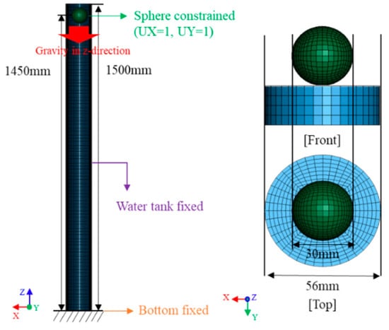
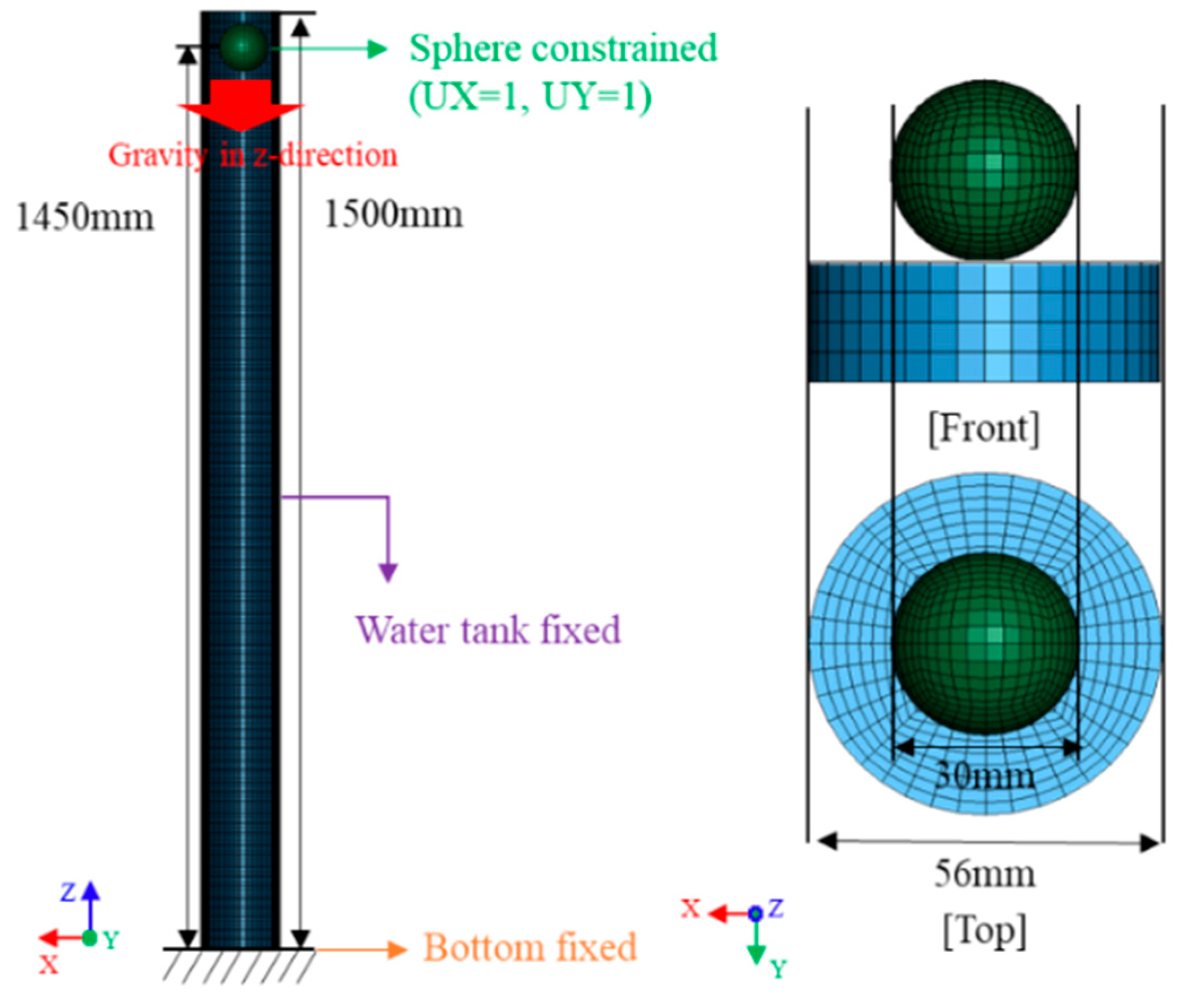
CFD analysis obtained for a water-dropping sphere in a narrow cylinder using the ADINA engineering simulation software program was compared with ANSYS/LS-DYNA computation. Modeling information, such as sphere dimensions, boundary constraints, computational time, was obtained from the reference [9,10,11]. Figure 2 shows the ANSYS/LS-DYNA FE model. The water domain was performed using an Arbitrary Lagrangian-Eulerian (ALE) with an eight-node element to describe the 56 mm diameter and 1500 mm height of a narrow cylinder water tank. The 30 mm diameter sphere was located at a height of 1450 mm above the ground. The 0.11 kg sphere is composed of steel having a density of 7795 kg/m3 and was modeled as a rigid Lagrangian with an eight-node solid element.
Figure 2.
FE model for the water-dropping sphere.
A 3 mm-sized mesh size was used for the sphere while the mesh size for the water was varied from 2 to 5 mm from the inner to outer line. The sphere and water domain contain 8000 and 138,000 elements, respectively. All external surfaces and bottom of the water tank were fixed. The only force of gravity that was considered was in the z-direction. Constraining the sphere to the x and y directions allowed for motion in the z-direction. The Lagrangian model of the sphere overlaps with the ALE water meshes. Their intersection should be detected and their interactions can be attributed to the Lagrangian element remapping on the moving ALE mesh.
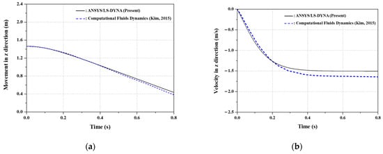
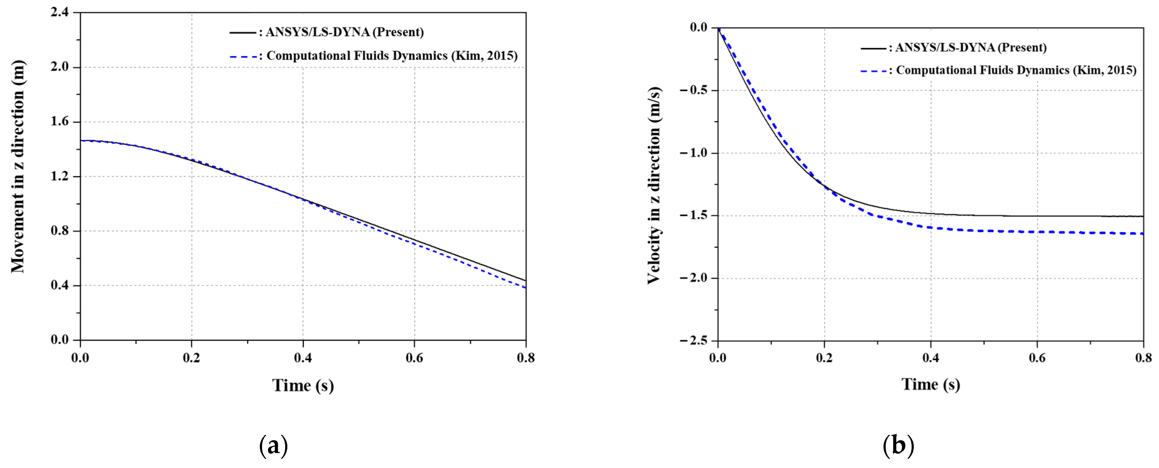
The movement and velocity of the sphere in the z-direction were compared between CFD and ANSYS/LS-DYNA. The overall difference can be observed in Figure 3. For movement in the z-direction, the same values are observed for until reaching 0.4 s, after which the gap between models increased. The difference at 0.8 s is about 9.75%. Velocity in the z-direction has a slight difference from the starting point, though a similar trend is observed between methods that became constant after 0.4 s and the difference at the termination time is about 9.05%. There appears to be a difference between the different simulation methods. However, similar trends are observed overall between methods and the difference is less than 10% and the computations used the same ALE model and EoS information for water.
Figure 3.
Comparison between CFD and FSI models: (a) Movement; (b) velocity in z direction.
2.3. Comparison with Experimental Model
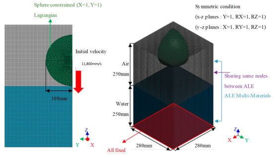
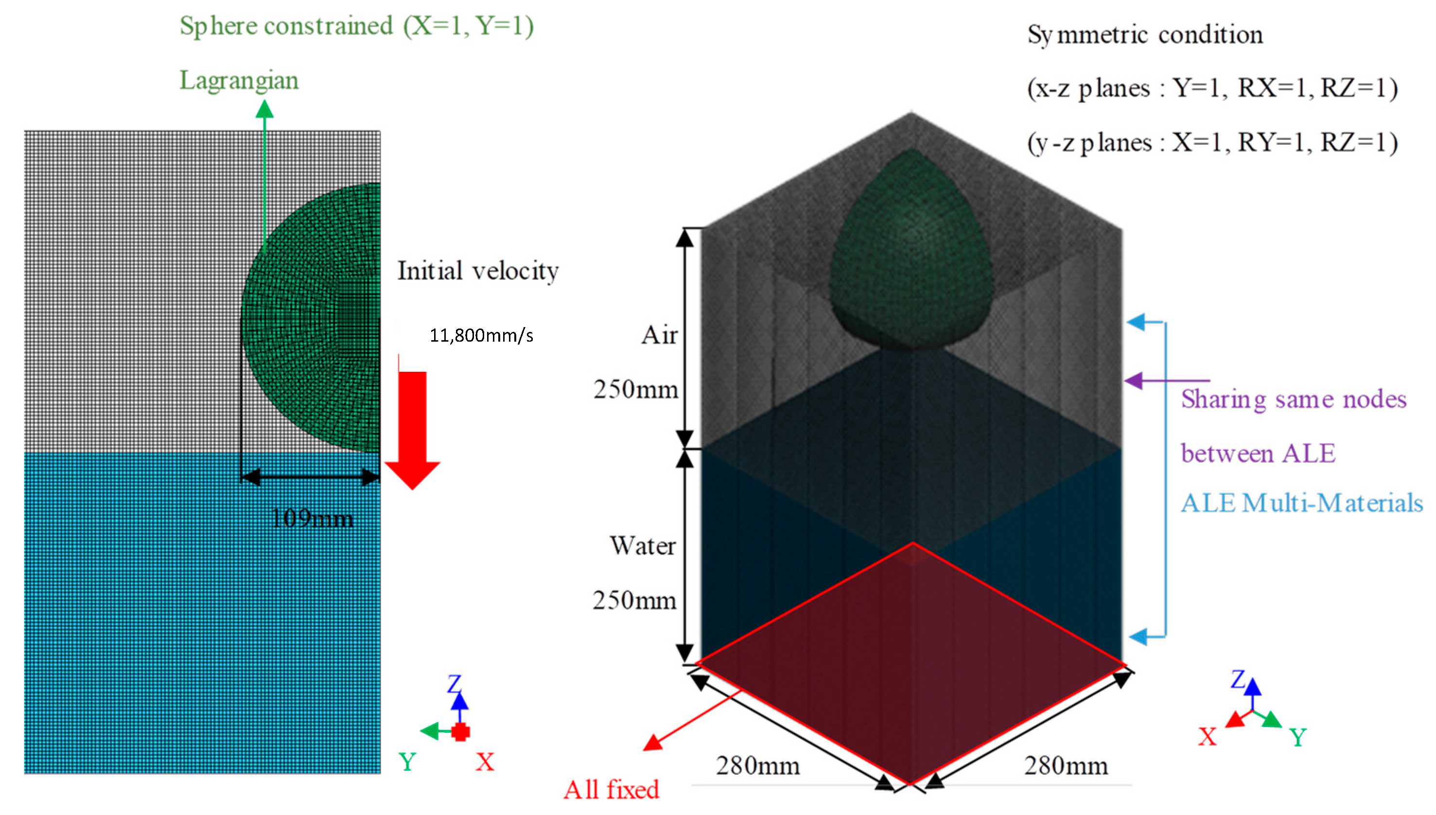
Many studies focused on a sphere falling in two fluids (air and water) [13,14,21]. Troesch and Kang [13] performed an experimental test to examine the hydrodynamic impact of a falling sphere. They compared the acceleration of the falling body with a theoretical model. Bisagni and Pigazzini [21] conducted numerical simulations of a vertical drop of a rigid sphere into water [13] using the Lagrangian, Smoothed Particle Hydrodynamics (SPH), and a hybrid Lagrangian—SPH model. Among the investigated models, ALE demonstrated a similar trend as experimental results, although it underestimated the first acceleration peak. Toso [14] examined multiple numerical techniques as a function of the mesh size effect, water tank size, and the effect of symmetry conditions. As per the work of Toso, there was no acceleration difference between full, half, and quarter-scale in the sphere drop analysis. As shown in Figure 4, the same modeling extents, boundary conditions, and element size of that work were adopted.
Figure 4.
FE model for the air-water-dropping sphere.
A rigid sphere with a radius of 109 mm and a 3.76 kg-sized mass was modeled by the Lagrangian model with a 10 mm-sized mesh size. The sphere was dropped in water in the vertical direction with an initial velocity of 11,800 m/s. The fluid was modeled using an eight-node solid ALE model with a 3 mm-sized mesh size. Water and air were described using EoS and including hydrostatic pressure. The bottom of the water was constrained, and symmetric conditions were applied to x-z and y-z planes. The dropping sphere was superimposed in water and air domain. Moreover, the two fluids shared the same nodes on their common boundary surfaces by applying the ALE multi-material option in ANSYS/LS-DYNA. The number of elements in air and water was 752,643; moreover, the number of elements in the sphere was 14,000.
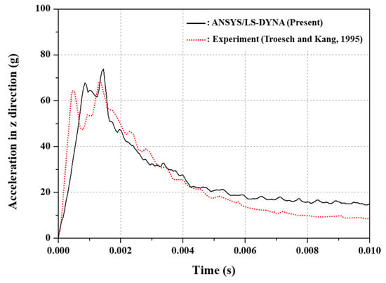
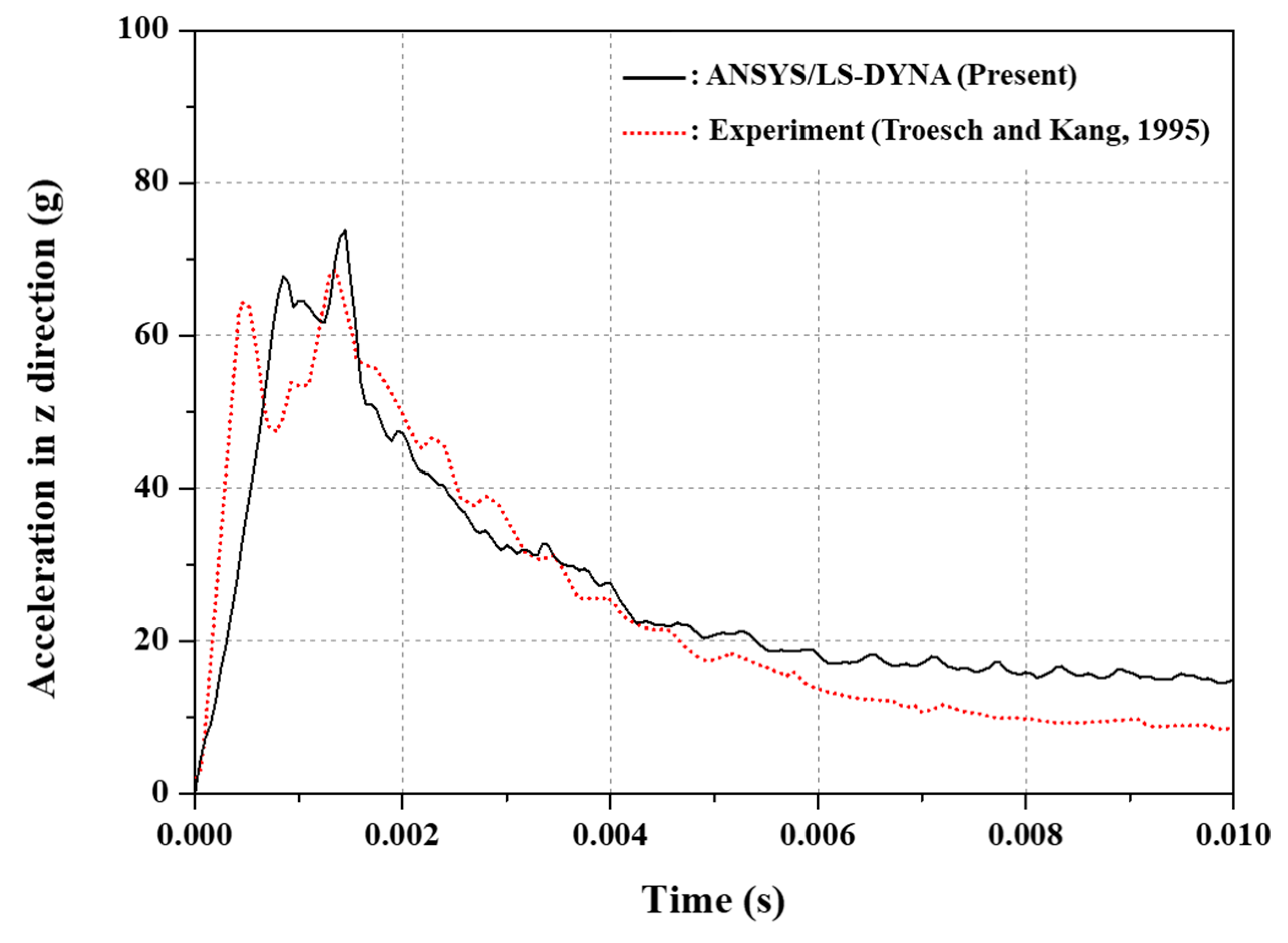
Figure 5 shows a comparison of the time acceleration of a sphere moving via two fluids. The sphere touched ground at around 0.01 s. A difference in values between both methods is observed for the entire time; however, the methods have similar trends, including two peak values wherein the second peak is slightly higher than the first. Moreover, the calculated values both decrease after the second peak. The difference in the slope of the first peak predictably describes the fluid using the EoS equations. Furthermore, it seems that the particle approximation of the water domain in the ALE model exhibits slightly stiffer behavior compared to the experiment. In terms of peak values, the discrepancy of the maximum accelerations compared with the experiment were 5.08% and 7.72% for first and second peaks, respectively. Based on the two types of validation, multiple analytical options are utilized in Section 4.
Figure 5.
Comparison between test and FSI models.
3. Experiment for the Underwater Drop of a Crusher
3.1. Stone-Breaking Crusher
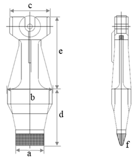
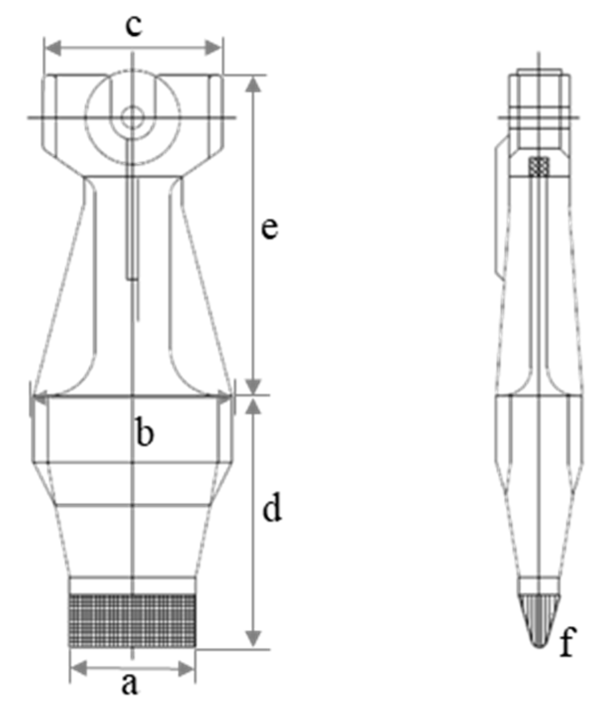
In this test, two different mass models of the crusher were used to confirm that the impact loads linearly increase with increase in mass. Table 3 shows the mass and volume of each crusher. The detailed 15-times scaled-down crusher models are presented in Figure 6. The dimension is noted as a-f and values are summarized in Table 4. A mass of 14.81 kg is a scaled-down 50 ton crusher and a 20.74 kg model is for a scaled-down 70 ton crusher. Generally, 5–50 ton crushers were used and the 70 ton model was re-drawn based on the 50 ton results. In this study, the 14.81 and 20.74 kg crushers are referred to as A and B, respectively.
Table 3.
Crusher model properties.
Figure 6.
Description of 15-times scaled-down crusher model.
Table 4.
Dimensions of crusher models.
3.2. Experimental Conditions
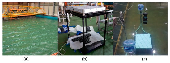
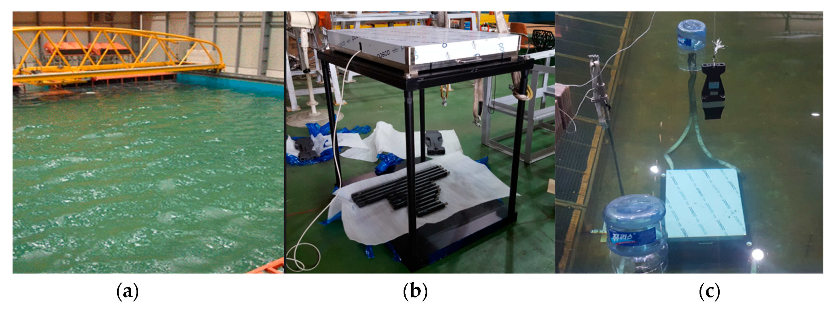
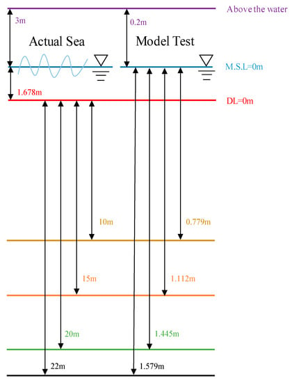
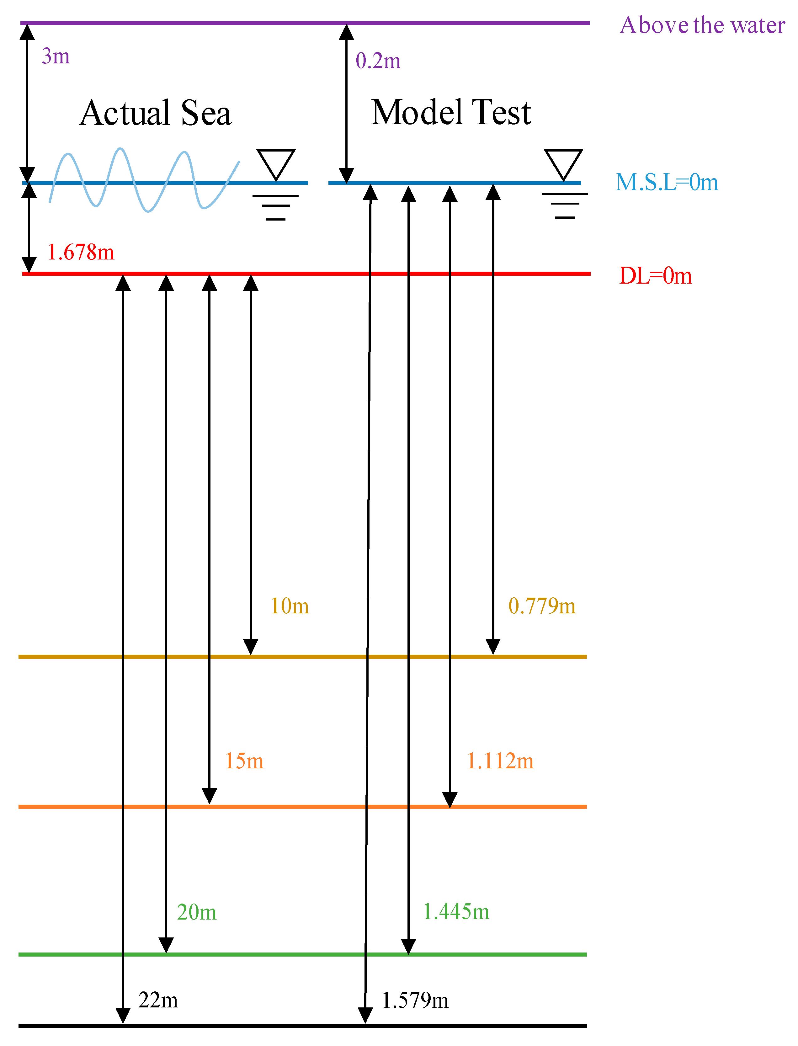
The RIMS in Korea conducted 15-times down-scaled drop tests for a breaking crusher in a water basin (28 × 22 × 3 m3), as shown in Figure 7a. The aim of this experiment was to evaluate the performance of the stone-breaking crusher in water and measure the impact force on ground. Experimental conditions included a temperature of 24 °C and relative humidity of 74.6%. All tests were conducted by considering conditions that were downscaled by 15 times with respect to the original conditions. Approximate Lowest Low Water (ALLW) was used as Datum Level (DL) in the test.
Figure 7.
Experimental environment: (a) Water basin; (b) load cell with sensor plate; (c) crusher.
A total of 16 cases were tested; actual and scaled-down test information are summarized in Table 5 and Figure 8. Four different water depths were evaluated—0.779, 1.112, 1.445, and 1.579 m. Moreover, air and water levels were described by having different falling positions—0.0 and 0.2 m. For each depth, tests were conducted three times. Impact force was measured using a sensor plate with an embedded load cell (max. capacity of 50,000 N and output of 500 Hz, ±5 V), as shown in Figure 7b. The sensor outputs a value using a strain gage via displacement, and the impact force is generated by the elasticity of strain gage. Figure 7c shows the load cell and crusher installed at the water basin.
Table 5.
Experimental scenarios.
Figure 8.
Actual and 1/15 scale-down experimental conditions.
3.3. Test Results
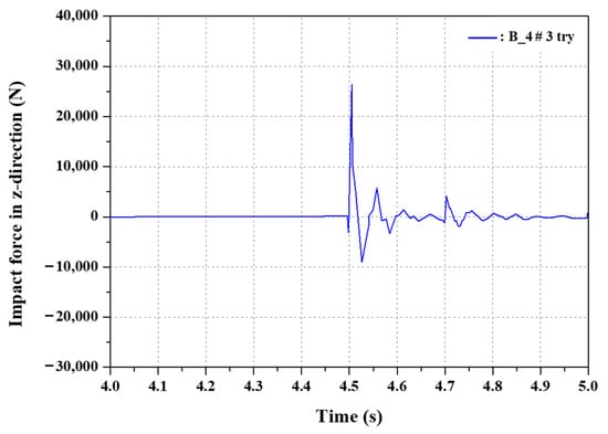
Figure 9 shows an example of the time–force history of the third run of B-4. It is observed that the force sharply increases when the crusher hits the sensor plate. Moreover, there was a fluctuation of load after contact. Table 6 summarizes the impact force when it shows the maximum value for all conditions. This suggests that the impact force generally tends to increase with increase in depth and weight of the crusher. As per Table 5, there is a gap between values at the same experimental condition. This discrepancy was attributed to a slightly different contact angle of the crusher when it struck the ground. Cases with data variability can be easily distinguished using the Coefficient of Variation (CoV; i.e., a high CoV means the experimental case lacks reliability by not demonstrating a consistent value). Therefore, numerical analysis was compared with the average of experimental values for each case.
Figure 9.
Example of time-load history for B-4 case.
Table 6.
Experimental results for all scenarios.
4. FSI Analysis for the Underwater Drop of a Crusher
4.1. Model Description and Analysis Settings
Numerical models for vertical falling of the crusher through fluid (air and water) were generated to compare impact force with the experimental results using FSI analysis in ANSYS/LS-DYNA [19]. Generally, the continuum motion description method used in FSI analysis is the ALE method [22,23,24]. The ALE method is a combination of Lagrangian and Eulerian techniques, which address the individual disadvantages of each method by maintaining advantages of both methods [10,25]. In this study, air and water were defined as an ALE multi-material, which tracks the interface of two materials in each element.
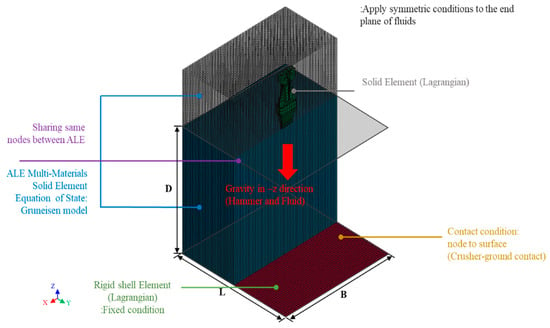
The same crusher geometry and water depth were used to describe experimental conditions for a vertical drop of the crusher into water. Figure 10 shows additional details on the numerical FE model and boundary and loading conditions. The fluid domain comprises B, L, and D as breadth, length, and depth, respectively. The crusher model was created by Hypermesh [26], whereas a FE model was generated after transferring all geometry information to ANSYS/LS-DYNA. The surrounding fluid domain was modeled as a rectangular parallelepiped in ANSYS/LS-DYNA. Moreover, a flat plate was attached at the bottom of the fluid to represent the ground.
Figure 10.
Analysis settings for numerical computation (B-2).
The crusher and ground were assumed to be a rigid material. As described in Section 2.1, the Grüneisen EoS model was used for water and air with the same coefficients. Air and water were considered one-point ALE multi-material elements. The crusher and ground were defined as Lagrangian, the crusher was a constant-stress solid element, and a four-node shell element was used for the ground. Common nodes on the boundaries of connecting ALE parts should be merged when one part of mesh flows to another. A coupling mechanism for FSI was implemented by defining the constrained Lagrange in solids, which was used to couple Lagrangian structures to ALE structures [18]. A crusher was assigned as slave part and ALE materials were set as master part.
Gravitational acceleration was added for representing the free fall of the crusher at the water level. The crusher allows only z movement by constraining the other degrees-of-freedom (DoF). When the crusher was vertically dropped in water, the contact angle of the crusher remained perpendicular to the ground. To show infinite fluid fields, symmetric boundary conditions in x-z and y-z planes of these two fluids were included. The ground was bonded to the fluid domain and all bottom nodes were fixed in six DoF. The surface-to-surface contact condition of the crusher and ground was defined. The Control_ALE command was used to set global control parameters for ALE. This command is required when using the ALE solid element. The use of default advection logic, the number of advection cycles, the advection technique, and the ALE smoothing weight factor were all set in Control_ALE.
4.2. Fluid Mesh Determination
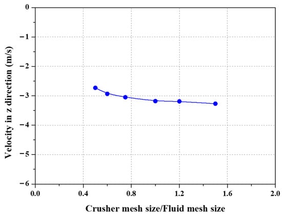
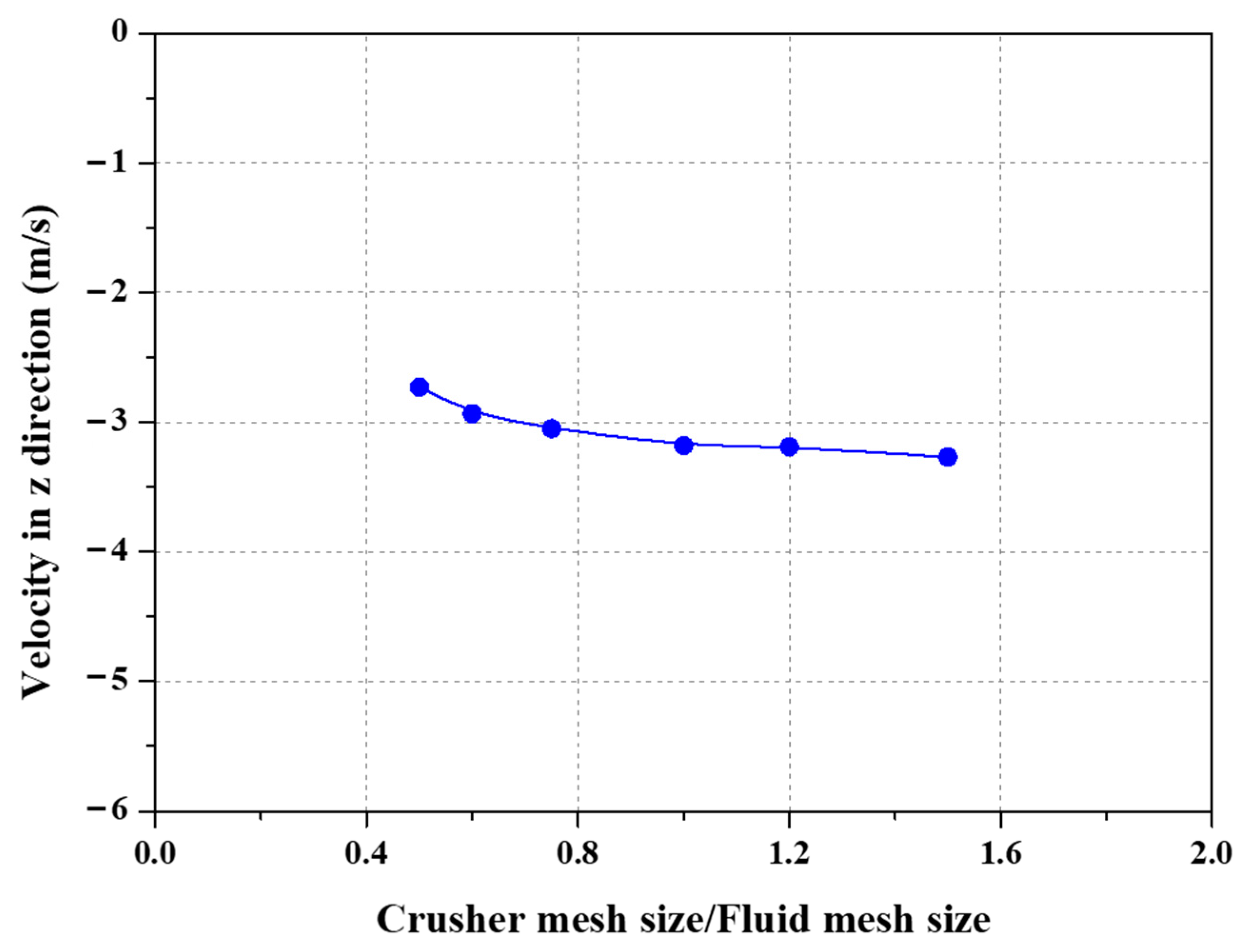
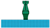
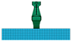
The ALE model must have a smaller mesh size to decrease the numerical error; however, as the size of the elements decreases, the number of elements and analysis time increase. Therefore, the element size must be adequate and a fluid mesh convergence test is important for this analysis. At the bottom edge of the crusher, the mesh size was set as 0.015 m. Fluid domain was constrained at B (or L) of 0.8 m and water depth of 0.779 m. The mesh in the fluid was varied from 0.01 to 0.03 m. Table 7 shows the number of nodes and elements (C/F is the ratio of element size for crusher (C) to fluid element size (F)). The computational time was not linearly increased by increasing C by F. Figure 11 shows the results of the mesh convergence test. The impact velocity decreased until C/F was 0.75 and then began to converge when it reached 1.00 because of the fluid element size convergence test. Consequently, the fluid element size was determined to be equal to the crusher element size.
Table 7.
The different mesh size in fluid.
Figure 11.
The effect of fluid mesh size.
4.3. Fluid Domain Determination
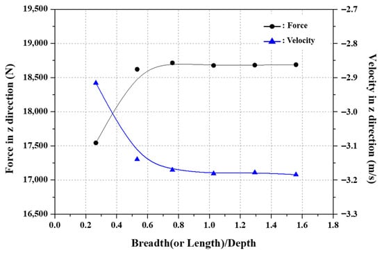
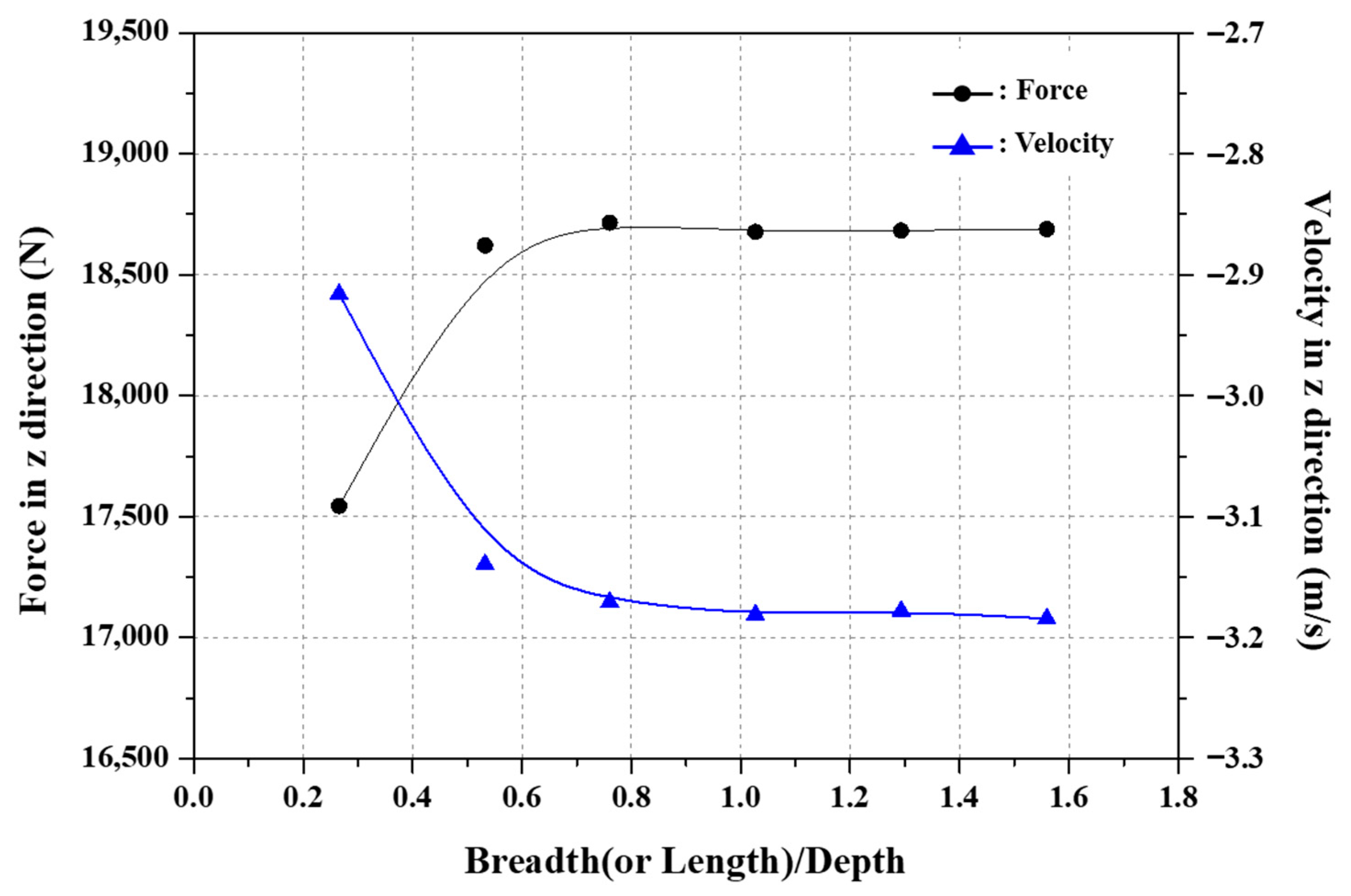
A fluid modeling area may be importantly influenced by the dimension of the crusher. As per Toso [14], the width of water tank should be at least twice the diameter of the falling model. To consider four water depths, the water domain was varied with water depth. To determine the size of water domain, several ratios of B(or L)/D (0.25 to 1.25) by D were examined at a water depth of 0.779 m. The defined fluid mesh size of 0.015 m was used in entire simulation. Table 8 shows the number of nodes, elements, modeling extent, and computational time for each analysis. As shown in Figure 12, the contact force and crusher velocity at the ground were compared. The impact force increases until B (or L)/D is 0.76, and then tends to converge from 1.03. To summarize, the fluid area size (B, L) was selected to be equal to the height of the fluid (D).
Table 8.
The various domain size of fluid.
Figure 12.
The effect of fluid domain size.
4.4. Results of Numerical Analysis
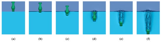
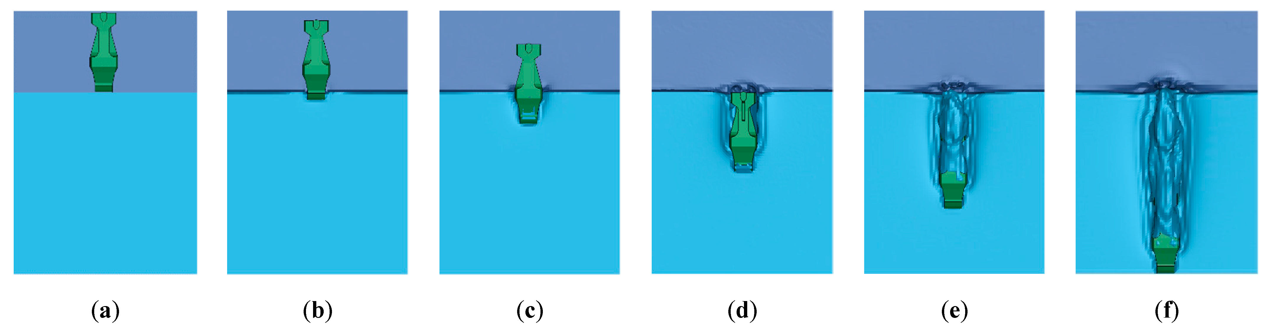
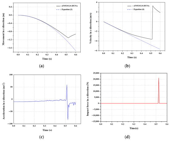
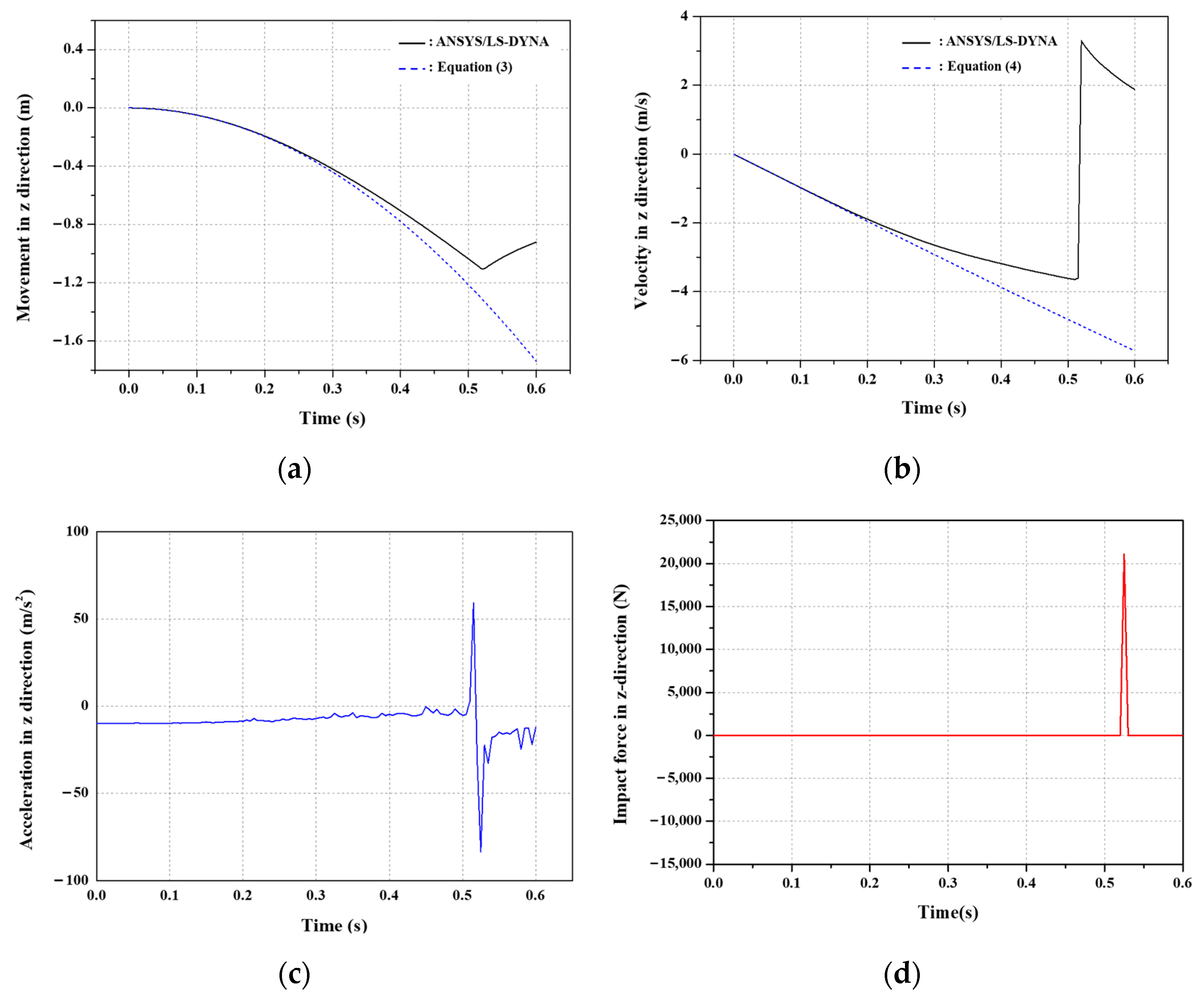
Figure 13 shows the movement in the vertical direction of the crusher and the flow change in fluid depending on time for the B-2 condition. The crusher reaches the ground at roughly 0.52 s. Additionally, it can be confirmed that the movement at touching time is coincident with the considered water depth of 1.112 m. The analysis results of the z-direction displacement, velocity, acceleration, and impact force of the B-2 condition were seen in Figure 14. According to Figure 14a,b, there was a rebound after hitting the ground, the direction was opposite around 0.52 s. It is slower than 0.476 s which is the time before hitting the ground if it is vacuum condition. Both graphs are compared with free-falling equations considering constant drag coefficient, as follows;
where is the difference between the mass of the crusher and the mass of water, g is the gravitational acceleration, w is the density of the water, A is the cross-sectional area of the crusher, t is the time. Cd of the drag coefficient was 0.668 based on the L by H of Model B using reference [27].
Figure 13.
Underwater movement of the crusher (B-2): (a) 0.000 s; (b) 0.100 s; (c) 0.200 s; (d) 0.325 s; (e) 0.400 s; (f) 0.520 s.
Figure 14.
The results of B-2 scenario: (a) Movement; (b) velocity; (c) acceleration; (d); impact force.
The gap is increasing around 0.3 s, which is the time that most parts of crusher were submerged underwater. It is obvious that it makes large difference because of considering constant drag coefficient, projected area and mass difference regardless of their position. It is difficult to set the drag coefficient for complex geometry model, like as the crusher. In addition, the velocity of FSI analysis at 0.52 s is −3.65 m/s. It is less than the value of −4.84 obtained from the equation. It is because that water resistance makes it slow. Figure 14c,d show acceleration and impact force. For acceleration, it shows the gravitational acceleration at the beginning, it remarkably increases when the crusher touches ground. Additionally, it is noted that it changes the direction when it rebounds. Impact force was measured from the contact force between the crusher and ground in time history curves. The acquired maximum value of contact force was dealt with impact force between the crusher and sensor plate in experimental models. For rigid ground, there is no penetration on the ground, the higher impact force was observed. In addition, it bounces back, the impact force is even greater because of the greater change in momentum.
4.5. Comparison between Experimental and Numerical Results
Table 9 shows the impact force of numerical and experimental results for 16 different cases. For numerical computations, the impact force gradually increased by increase in water depth and crusher model. Moreover, the impact force of a crusher dropping from air level is slightly larger than that at water level; however, this increase in trend was gradual with increase in water depth. For model B, the impact force does not linearly increase with increase in weight; there is a different ratio in each case; however, the average value is ~38% and is less than the weight increase of 40%. Therefore, the impact force of the original model does not have 15 times the impact force of the 15-times scaled-down model. An exact impact force should be measured from the original model size and water depth.
Table 9.
Summary of experimental and numerical analysis results.
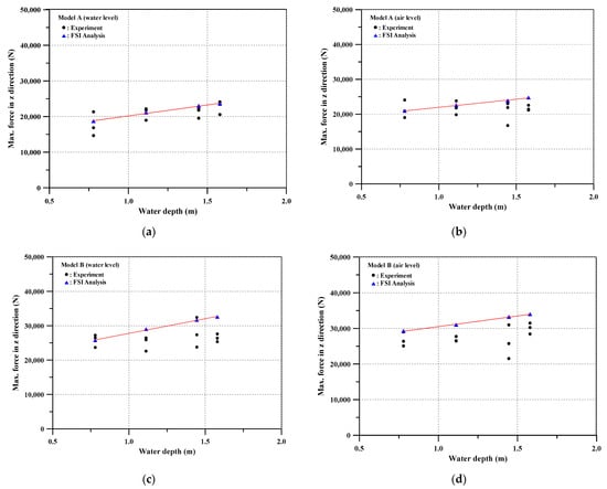
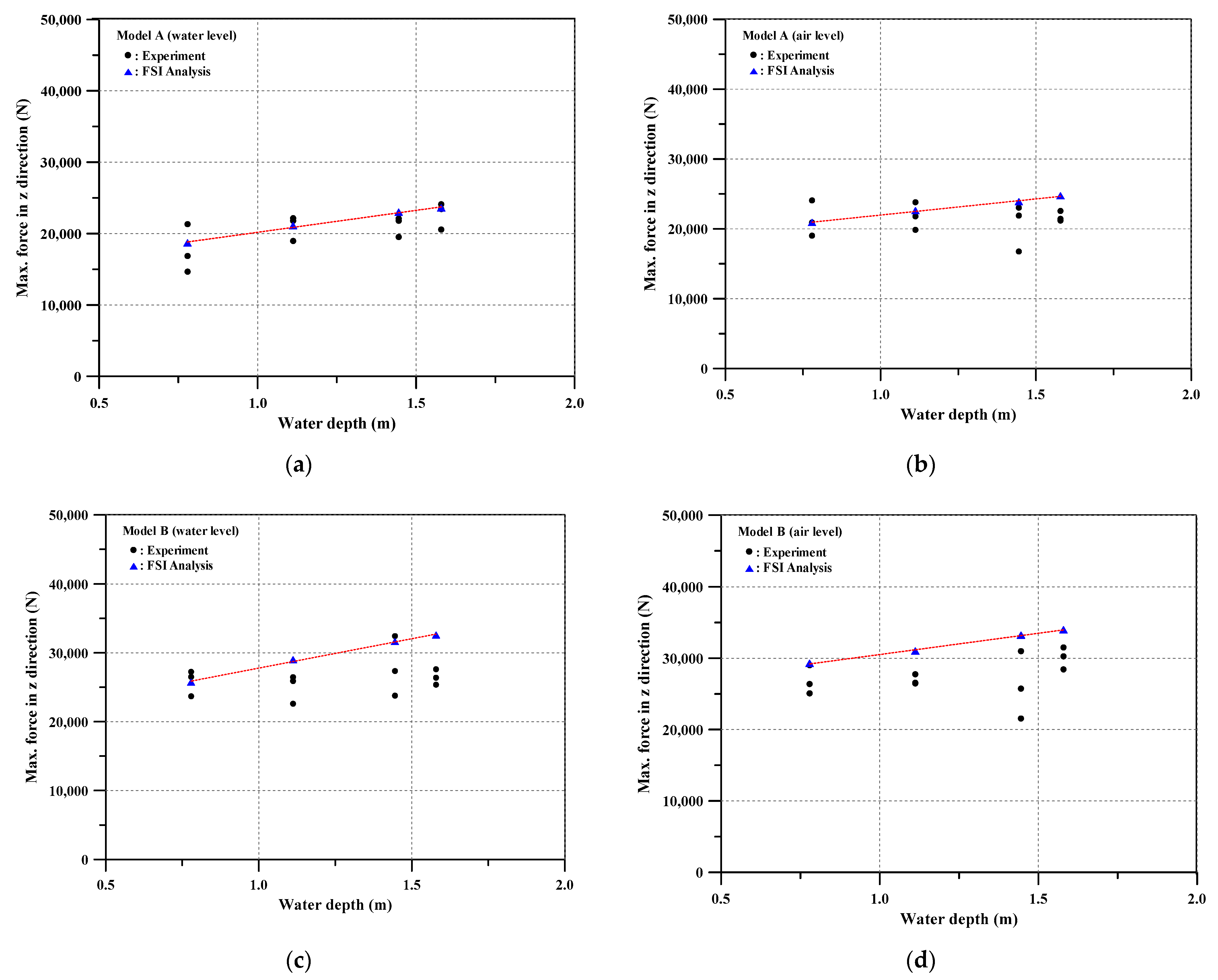
Figure 15 shows a comparison between experimental data and numerical values for impact force model A has much better agreement between experimental and numerical values compared to model B. This is because all numerical settings were determined for the model A condition; therefore, a higher error was recorded for model B. Certain cases, such as A-7, B-3, and B-7, have a higher COV and lead to larger errors. For A-7, A-8, B-2, B-4, and B-7, the average impact force was lower at lower water depth. In particular, the air level dropping case for A-7, A-8, and B-7 show lower impact force than for that at the water level. The increase in water depth has a higher probability to change the angle of attack of the crusher when it hits the ground, thus producing greater variability between each test and leads to an increase in difference between numerical and experimental data. However, the error could be dramatically reduced by comparing the maximum value of experimental and numerical values, for example, the error is 7.25% for B-7 (i.e., a reduction of ~20%). If comparison is assumed to be changed to maximum and compared to the LS-DYNA result, the error could be 7.25% for B-7. Therefore, the test should confirm the angle of impact of hitting the object for improved comparison. This is our next step for examining the effect of the angle of impact on the impact force.
Figure 15.
Comparison between experimental and numerical impact force: (a) Model A—water level; (b) Model A—air level; (c) Model B—water level; (d) Model B—air level.
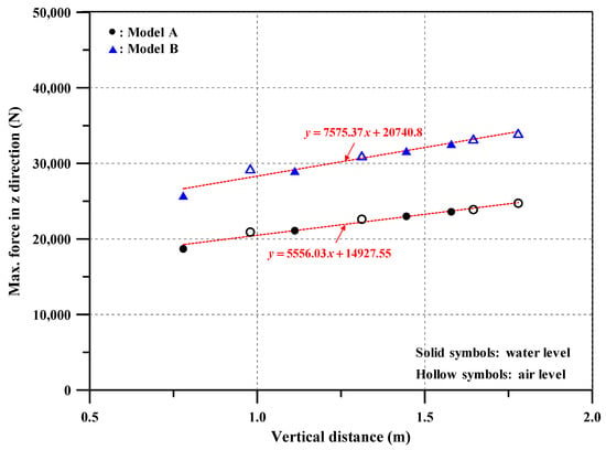
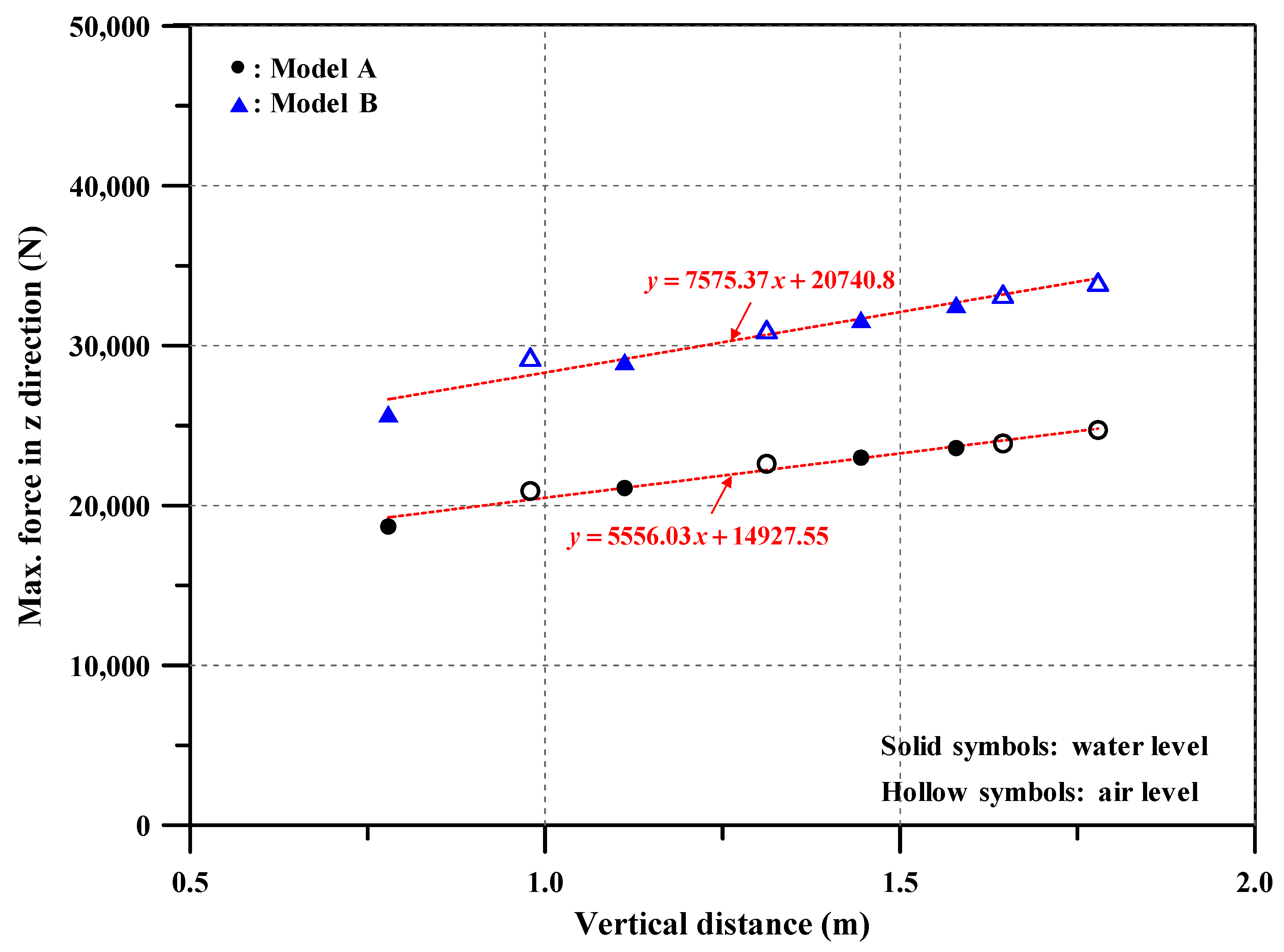
An additional graph was drawn for combining all numerical results in Figure 16. The axis of X represents the vertical distance from ground regardless of water depth. Therefore, drop point of air level has 0.2 m longer distance than water level. They show a linear relationship in the case of same model size. The linear equation was marked at the graph. It means that the impact force for specific shallow water depth could be predicted if the model is the same. But, it is not suitable for deeper water depth owing to increases of water resistance. Therefore, it is needed to find the critical depth which transits from linear to nonlinear tendency.
Figure 16.
Numerical results according to vertical distance.
5. Conclusions
This study aimed to understand the characteristics of a crusher in water and predict the impact force on ground using experimental and numerical methods. Based on the study, the following conclusions can be obtained:
- Experimental tests for two different scaled-down models and multiple water depths with two different dropping levels were conducted to confirm that the impact loads linearly increase with increase in mass. In addition, this will be a good reference for validating numerical methods on dropping object into the water.
- Numerical techniques using FSI analysis for a free-falling crusher were established by applying the ALE element and Grüneisen EoS to the fluid models. To increase accuracy, two validation methods comprising CFD and experiment models for a rigid sphere were performed. Furthermore, modeling size and extent were determined by multiple computations.
- Model size and water depth are the most influential factors to increase impact force on the ground. The impact force increases as water depth increases. Moreover, the air-level drop shows typically greater impact force than that of a water-level drop. Higher impact force was measured for model B than A; however, there is no specific ratio between them. Therefore, there is no linear relationship based on model weight or, in other words, there is no dynamic similarity of impact force between the model and prototype.
- Similar trends were observed between numerical and experimental data. Certain cases demonstrate good agreement while others have >20% error because there is large variance in experimental data. In particular, there is a higher CoV for increase in water depths. Moreover, certain cases do not show constant results because of angular rotation between the crusher and ground when the crusher hits the ground.
Further studies will include performing drop tests and measuring the impact force of simple dropping objects (sphere and cone) in a water tank to examine the effect of the impact angle on the ground.
Author Contributions
Conceptualization, J.M.S. and S.H.K.; methodology, J.M.S. and S.H.K.; software, J.W.K. and J.M.S. validation, J.W.K. and J.M.S.; formal analysis, J.W.K. and J.M.S.; investigation, S.H.K.; resources, S.H.K.; data curation, S.H.K. and J.M.S.; Writing—original draft preparation, J.W.K. and J.M.S.; writing—review and editing, J.W.K. and J.M.S.; visualization, J.W.K.; supervision, J.M.S.; project administration, J.M.S. All authors have read and agreed to the published version of the manuscript.
Funding
This research received no external funding.
Institutional Review Board Statement
Not applicable.
Informed Consent Statement
Not applicable.
Data Availability Statement
The data presented in this study are available in this article (tables and figures).
Acknowledgments
The first author gratefully acknowledges publishing support by a grant from Brain Korea 21 Program for Leading Universities and Students (BK21 FOUR) MADEC Marine Designeering Education Research Group. Ji Wo Kim acknowledges funding support for X-mind Corps program of National Research Foundation of Korea (NRF) by the Ministry of Science, ICT (No. 2019H1D8A1105564) in South Korea.
Conflicts of Interest
The authors declare no conflict of interest.
Abbreviations
| ALE | Arbitrary Lagrangian-Eulerian |
| COV | Coefficient of Variation |
| CFD | Computational Fluid Dynamics |
| DoF | Degree of Freedom |
| FE | Finite Element |
| MSL | Mean Sea Level |
| RIMS | Research Institute of Medium and Small Shipbuilding |
| ALLW | Approximate Lowest Low Water |
| CEL | Coupled Eulerian-Lagrangian |
| DL | Datum Level |
| EoS | Equation of State |
| FSI | Fluid-Structure Interaction |
| RANS | Reynolds-averaged Navier-Stokes |
| SPH | Smoothed Particle Hydrodynamics |
References
- Bray, R.N.; Richard, N.; Bates, A.D.; Land, J.M. Dredging: A Handbook for Engineers; Arnold: London, UK, 1997. [Google Scholar]
- Keevin, T.M.; Hempen, G.L. The Environmental Effects of Underwater Explosions with Methods to Mitigate Impacts; U.S. Army Corps of Engineers: St. Louis, MO, USA, 1997.
- Tripathy, G.R.; Shirke, R.R. Underwater drilling and blasting for hard rock dredging in indian ports—A case study. Aquat. Procedia 2015, 4, 248–255. [Google Scholar] [CrossRef] [Scilit]
- Nikolov, S.A. performance model for impact crushers. Miner. Eng. 2002, 15, 715–721. [Google Scholar] [CrossRef] [Scilit]
- Cleary, P.W.; Sinnott, M.D.; Morrison, R.D.; Cummins, S.; Delaney, G.W. Analysis of cone crusher performance with changes in material properties and operating conditions using DEM. Miner. Eng. 2017, 100, 49–70. [Google Scholar] [CrossRef] [Scilit]
- Kim, S.J.; Kõrgersaara, M.; Ahmadi, N.; Taimuri, G.; Kujala, P.; Hirdaris, S. The influence of fluid structure interaction modelling on the dynamic response of ships subject to collision and grounding. Mar. Struct. 2021, 75, 102875. [Google Scholar] [CrossRef] [Scilit]
- Lee, S.; Zhao, T.; Nam, J. Structural safety assessment of ship collision and grounding using FSI analysis technique. In Proceedings of the 6th International Conference on Collision and Grounding of Ships and Offshore Structures, ICCGS, Trondheim, Norway, 17–19 June 2013; Jørgan Amdahl. CRC Press/Balkema: Boca Raton, FL, USA, 2013; pp. 197–204. [Google Scholar]
- Song, M.; Ma, J.; Huang, Y. Fluid-structure interaction analysis of ship-ship collisions. Mar. Struct. 2017, 55, 121–136. [Google Scholar] [CrossRef] [Scilit]
- Kim, J.Y. A Study on Unsteady Drag Coefficient of Free Falling Structure in the Water. Ph.D. Thesis, Chungnam National University, Daejeon, Korea, 2015. [Google Scholar]
- Jang, G.H.; Kim, J.H.; Song, C.Y. Comparison of Underwater Drop Characteristics for Hazard Apparatuses on Subsea Cable Using Fluid-Structure Interaction Analysis. J. Ocean. Eng. Technol. 2018, 32, 324–332. [Google Scholar] [CrossRef] [Scilit]
- Kim, J.Y.; Yoon, K.H.; Oh, S.H.; Ko, S.H. CFD Analysis to Estimate Drop Time and Impact Velocity of a Control Rod Assembly in the Sodium Cooled Faster Reactor. KSFM J. Fluid Mach. 2015, 18, 5–11. [Google Scholar] [CrossRef] [Scilit]
- Yu, P.; Shen, C.; Zhen, C.; Tang, H.; Wang, T. Parametric Study on the Free-Fall Water Entry of a Sphere by Using the RANS Method. J. Mar. Sci. Eng. 2019, 5, 122. [Google Scholar] [CrossRef] [Scilit]
- Troesch, A.W.; Kang, C. Hydrodynamic impact loads on three-dimensional bodies. In Proceedings of the Symposium on Naval Hydrodynamics, Berkeley, CA, USA, 13–16 July 1986. [Google Scholar]
- Toso, N.R.S. Contribution to the Modelling and Simulation of Aircraft Structures Impacting on Water. Ph.D. Thesis, University Stuttgart, Stuttgart, Germany, 2009. [Google Scholar]
- Abelev, A.V.; Valent, P.J.; Holland, K.T. Behavior of a large cylinder in free-fall through water. IEEE J. Ocean. Eng. 2007, 32, 10–20. [Google Scholar] [CrossRef] [Scilit]
- Fallah-Kharmiani, S.; Khozeymeh-Nezhad, H.; Niazmand, H. Numerical study of free-fall cylinder water entry using an efficient three-phase lattice Boltzmann method with automatic interface capturing capability. Ocean. Eng. 2021, 235, 109328. [Google Scholar] [CrossRef] [Scilit]
- ANSYS/LS-DYNA. In ANSYS/LS-DYNA 2020 R1; ANSYS Inc: Canonsburg, PA, USA, 2020.
- Olovsson, L.; Souli, M.; Do, I. LS-DYNA-ALE capabilities (Arbitrary-Lagrangian-Eulerian) Fluid-Structure Interaction Modeling. Available online: https://ftp.lstc.com/anonymous/outgoing/jday/aletutorial-278p.pdf (accessed on 8 November 2021).
- LS-DYNA. In LS-DYNA Keywords User’s Manual, 12th ed.; Livermore Software Technology Corporation: Livermore, CA, USA, 2020.
- Khazraiyan, N.; Gerami, N.D.; Damircheli, M. Numerical Simulation of Fluid-Structure Interaction and its Application in Impact of Low-Velocity Projectiles with Water Surface. ADMT J. 2015, 8, 81–90. [Google Scholar]
- Bisagni, C.; Pigazzini, M.S. Modelling strategies for numerical simulation of aircraft ditching. Int. J. Crashworthiness 2018, 23, 377–394. [Google Scholar] [CrossRef] [Scilit]
- Benson, D.J. An efficient, accurate, simple ALE method for nonlinear finite element programs. Comput. Methods Appl. Mech. Eng. 1989, 72, 305–350. [Google Scholar] [CrossRef] [Scilit]
- Truong, D.D.; Jang, B.S.; Ju, H.B.; Han, S.W. Prediction of slamming pressure considering fluid-structure interaction. Part II: Derivation of empirical formulations. Mar. Struct. 2021, 75, 102700. [Google Scholar] [CrossRef] [Scilit]
- Souli, M.; Ouahsine, A.; Lewin, L. ALE formulation for Fluid-Structure interaction problems. Comput. Methods Appl. Mech. Eng. 2000, 190, 659–675. [Google Scholar] [CrossRef] [Scilit]
- Jang, I.H. Sloshing Response Analysis of LNG Carrier Tank Using Fluid-Structure Interaction Analysis Technique of LS-DYNA3D. Master’s Thesis, Korea Maritime and Ocean University, Busan, Korea, 2007. [Google Scholar]
- Hypermesh. HyperWorks14.0 User’s Guide; Altair: Troy, MI, USA, 2020. [Google Scholar]
- White, F.M. Fluid Mechanics, 7th ed.; Mcgraw-Hill College: New York, NY, USA, 2009. [Google Scholar]




Publisher’s Note: MDPI stays neutral with regard to jurisdictional claims in published maps and institutional affiliations. |
© 2021 by the authors. Licensee MDPI, Basel, Switzerland. This article is an open access article distributed under the terms and conditions of the Creative Commons Attribution (CC BY) license (https://creativecommons.org/licenses/by/4.0/).