Convolution Neural Network for the Prediction of Cochlodinium polykrikoides Bloom in the South Sea of Korea

Abstract

In this study, the occurrence of Cochlodinium polykrikoides bloom was predicted based on spatial information. The South Sea of Korea (SSK), where C. polykrikoides bloom occurs every year, was divided into three concentrated areas. For each domain, the optimal model configuration was determined by designing a verification experiment with 1–3 convolutional neural network (CNN) layers and 50–300 training times. Finally, we predicted the occurrence of C. polykrikoides bloom based on 3 CNN layers and 300 training times that showed the best results. The experimental results for the three areas showed that the average pixel accuracy was 96.22%, mean accuracy was 91.55%, mean IU was 81.5%, and frequency weighted IU was 84.57%, all of which showed above 80% prediction accuracy, indicating the achievement of appropriate performance. Our results show that the occurrence of C. polykrikoides bloom can be derived from atmosphere and ocean forecast information.

1. Introduction

Harmful algal bloom (HAB) is a common phenomenon that has been recorded in the past, but in recent years, the number and duration of occurrences have increased due to human influence [1]. Particularly, in the South Sea of Korea (SSK), where aquaculture farms are densely populated, the HABs that repeatedly occur almost every year cause economic damages to the aquaculture industry. HAB outbreaks in the SSK were mainly caused by diatoms in the early 1990s, but after 1995, Cochlodinium polykrikoides with dinoflagellate has become the primary cause [2,3,4]. C. polykrikoides blooms mainly occurring between Naro-do and Namhae-do are not limited locally and spread to the entire SSK, the East Sea (Sea of Japan), and the Yellow Sea coasts, causing significant damage [3,5]. Therefore, a novel method is required because early detection and monitoring are limited by the investigation of only the local area.

HAB monitoring has been conducted by vessel surveys, coastal visual observations, and aerial surveys for a long time. In Korea, the National Institute of Fisheries Science (NIFS) has conducted such studies as the central institution since the 1970s. However, because in-situ observation is manual-labor-intensive and expensive, there is a limit concerning monitoring the entire sea, and therefore, the method of remote sensing has attracted considerable attention. Because remote sensing has the advantage of affording wide-area information immediately, research using satellites has been actively conducted, and various HAB detection algorithms have been developed. However, HABs occur mainly on the coast, and high concentrations of suspended matter and dissolved organic matter on the coast degrade the quality of satellite data [6], making it challenging to detect HABs [7,8].

HAB prediction is an essential step in minimizing economic losses. Until now, most efforts have been made to predict the scale and migration of HABs and reduce damage through ecological research and monitoring of harmful algae. However, it is difficult to predict and prepare for HABs because the cause or process of occurrence has not yet been clearly identified [1].

It is extremely difficult to predict HABs because these phenomena consist of highly complex physical, chemical, and biological processes. Physical prediction models encounter difficulties prescribing related variables and coefficients when predicting HABs; moreover, enormous computational resources are required for calculation [9]. Furthermore, the use of data-driven prediction methods have become increasingly common in the prediction of HABs [10,11,12].

In this study, we predict HABs using a correlation model of non-linear environmental and biological factors [5]. Bak et al. [13] proposed a method to determine the presence of HABs in the SSK by applying logistic regression and decision trees to satellite images. Bak et al. [14] predicted the occurrence of C. polykrikoides blooms in the SSK by constructing a deep neural network with eight hidden layers. Shin et al. [15] applied sea surface temperature (SST) and photosynthetically available radiation (PAR) to a deep neural network model of long short-term memory (LSTM) to predict the timing of C. polykrikoides bloom in the SSK; the results were five days ahead of the actual occurrence of HABs, therefore it could be used for early prediction. Kim et al. [16] constructed a U-Net convolution neural network model based on GOCI’s normalized water-leaving radiance (_nL_w) based on the red tide index (RI) of Shin et al. [17] and predicted HABs with 13% higher accuracy than that in the case of the four-band dataset in the six-band dataset.

Recently, with the development of advanced spatial image analysis and deep learning, research on the correlation between spatial information and phenomena has received considerable attention. Until now, the prediction of HAB occurrence using the model in the SSK has been studied with the remote sensing reflectance (R_rs) of the satellite as a parameter. Satellite R_rs may cause detection accuracy problems due to low data accuracy of the coast and high spectral similarity between HABs and turbid coastal water. Previous studies [13,14,15] showed that environmental parameters are closely related to the occurrence of C. polykrikoides. In this study, ocean and weather model data were used to predict the blooms of C. polykrikoides, the main species that cause HABs in the SSK. The spatial distribution was predicted using a convolutional neural network (CNN) model.

2. Data and Methods

2.1. C. polykrikoides Bloom Data

The C. polykrikoides occurrence prediction model was trained and verified using NIFS breaking news data (http://www.nifs.go.kr/red/main.red (accessed on 20 December 2021)). The C. polykrikoides observational data are based on vessel, land, and aerial surveillance results of the studies conducted by the NIFS, fisheries technology offices, and maritime security and safety headquarters (

Table 1. C. polykrikoides monitoring system in the SSK.

Type	Surveillance Area	Surveying Periods	Organization in Charge
Vessel surveillance	102 stations	March to November (one to two times per month)	NIFS
Land surveillance	130 stations	April to October (two times per week)	Fisheries technology offices
Aerial surveillance	Area where HABs occurs	On-demand	Korea Coast Guard

). In the C. polykrikoides blooms, observation time and location are recorded using GPS, and the density and water temperature are provided. In this study, we used the time and location of C. polykrikoides blooms. These data were mapped to a 3-km grid considering the minimum resolution of the marine and meteorological numerical model data. Based on the cumulative number of C. polykrikoides bloom occurrences per grid over the past 10 years (Figure 1), the predicted area of C. polykrikoides bloom occurrence is equally divided into three zones in the SSK because the characteristics of water masses are different based on the complex topography and islands (for example, Namhae-do and Geoje-do) in the South Coast of Korea [18]; this affects the location and timing of the occurrence of C. polykrikoides blooms [15,17].

2.2. Meteorological Data

Meteorological reanalysis data were obtained from the National Centers for Environmental Prediction (NCEP) Global Forecasting System (GFS, https://www.ncdc.noaa.gov/data-access/model-data/model-datasets/global-forcast-system-gfs (accessed on 20 December 2021)). GFS provides dozens of atmospheric and soil parameters. The spatial resolution was 0.5°, and prediction information was produced at 1h intervals for the first 120 h and provided at 3h intervals for 5–16 days. From the GFS data, we selected 13 parameters for the input data for the growth and movement prediction of C. polykrikoides (

Table 2. Meteorological input data from NCEP GFS for the HAB prediction model.

Number	Level	Valid Time	Parameter	Description
435	2 m above ground	3h forecast	TMP	Temperature (K)
438	2 m above ground	3h forecast	RH	Relative Humidity (%)
442	10 m above ground	3h forecast	UGRD	U-Component of Winds (m/s)
443	10 m above ground	3h forecast	VGRD	V-Component of Winds (m/s)
446	Surface	3h forecast	PRATE	Precipitation Rate (km/m2/s)
462	Surface	0–3 h average	LHTFL	Latent Heat Net Flux (W/m2)
463	Surface	0–3 h average	SHFTL	Sensible Heat Net Flux (W/m2)
465	Surface	0–3 h average	UFLX	Momentum Flux, U-Component (N/M2)
466	Surface	0–3 h average	VFLX	Momentum Flux, V-Component (N/M2)
497	Surface	0–3 h average	DSWRF	Downward Short-Wave Radiation Flux(W/m2)
498	Surface	0–3 h average	DLWRF	Downward Long-Wave Radiation Flux (W/m2)
499	Surface	0–3 h average	USWRF	Upward Short-Wave Radiation Flux (W/m2)
500	Surface	0–3 h average	ULWRF	Upward Long-Wave Radiation Flux (W/m2)

). Because the C. polykrikoides occurrence information is provided daily, the meteorological model data were also averaged daily. Only the regions shown in Figure 1 were extracted for efficient time management and tensor optimization, when training the model.

2.3. Oceanographic Data

The temperature and salinity of GLBv0.08 provided by the Center for Ocean-Atmospheric Prediction Studies (COAPS) Hybrid Coordinate Ocean Model (HYCOM) (https://www.hycom.org/ (accessed on 20 December 2021)) were used as the ocean reanalysis data. C. polykrikoides blooms occur in a wide range of water temperatures and salinities [19,20,21,22,23,24]. COAPS HYCOM provides a spatial resolution of 0.08° from 40° S to 40° N. The HYCOM data are provided in standard z-levels of 40 layers from the sea surface to the seafloor. We used sea surface height (SSH), eastward velocity, northward velocity, temperature, and salinity fields as inputs for the HAB prediction model.

2.4. Model Structure and Training

Deep learning is a subfield of machine learning in which data clustering and classification are performed after extracting key features of data through the high-level abstraction of training data using a nonlinear transformation technique. Various neural networks based on Convolutional Neural Network (CNN) show excellent performance in the prediction or detection of ocean and weather parameters [25,26,27,28].

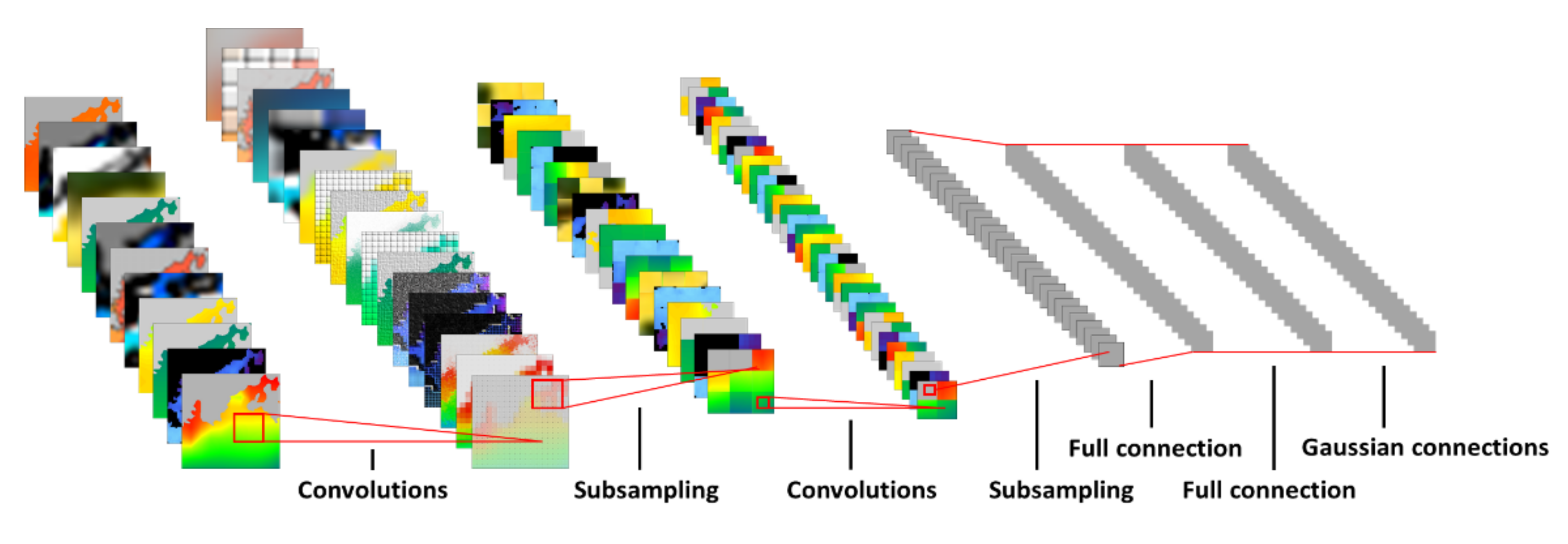
2.4.1. Convolution Neural Network

CNN is a deep learning model that was proposed by Lecun et al. [29] for handwriting-character recognition and is a model that mimics the human optic nerve structure processing vision information. Among all the deep learning algorithms, the CNN model is specialized for image processing, and the CNN structure is shown in Figure 2. The image input to the input layer is converted into a number for each pixel and is saved as a feature map from which the features of the image are extracted through a filter in the convolution layer. In this case, various features of the image may be extracted according to the filter size and the calculation method used. In the next pooling layer, the size of the image is reduced through max pooling, reducing the amount of computation, and transferring the main features of the image to the next layer. After repeating this process, in fully connected, the three-dimensional (3D) value is converted to 1D to determine whether the object image to be identified matches, and the identification result is output at the last output layer. In this study, two-dimensional(2D) CNN (CONV2D) automatically extracts the features of the object to be recognized from the learning image by alternately performing the operations at the convolution layer and pooling layer to extract the 2D features. In this study, using the CNN model, a model capable of spatially discriminating the occurrence of C. polykrikoides blooms from the 2D information of the meteorological model and ocean model was developed and verified.

To evaluate the accuracy according to the number of CNN layers and the number of training times, the root mean squared error (RMSE) and prediction accuracy (ACC) were used to evaluate the validation loss and validation accuracy. The indices of the accuracy evaluation are as follows:

$$\mathrm{RMSE}=\frac{{{\displaystyle \sum }}_{i=1}^n{(X_{obs,i}-X_{model,i})}^2}{n}$$

(1)

$$\mathrm{ACC}=1-\frac{{{\displaystyle \sum }}_{i=1}^n\left(\frac{\left|X_{model,i}-X_{obs,i}\right|}{X_{obs,i}}\right)}{n}$$

(2)

where X_obs,i is the observed value, X_model,i is the value modeled at position i, i is the low column number, n is the number of pixels to be predicted, and n = M × N. RMSE represents the absolute error, whereas ACC represents the relative accuracy. A smaller RMSE indicates a higher performance, and the opposite is true for ACC. Spatially averaged RMSE and ACC were used for areal prediction.

The time interval of the prediction model is one day, following the input parameters from ocean and weather numerical models. Because we used one-to-one forecast neural networks, HABs prediction period is equal to the ocean and weather numerical forecast models.

For neural network optimization, we investigated an optimal number of training epochs. The performance increased up to epoch 300, but deteriorated after the optimal epoch number. This showed that better convergence and accuracy could not be obtained in the number of training more than 300 times, due to the overfitting problem.

Before experimenting, the effect of predicting the occurrence of C. polykrikoides blooms was evaluated based on pixel accuracy, mean accuracy, mean Intersection over Union (IU), and frequency weighted IU as the indicators of the accuracy of the experimental results. The indices of the accuracy evaluation are as follows:

$$\mathrm{pixel} \mathrm{accuracy}={{\displaystyle \sum }}_i{n}_{ii}/{{\displaystyle \sum }}_i{t}_i$$

(3)

$$\mathrm{mean} \mathrm{accuracy}=\left(1/n_{cl}\right){{\displaystyle \sum }}_i{n}_{ii}/t_i$$

(4)

$$\mathrm{mean} \mathrm{IU}=\left(1/n_{cl}\right){{\displaystyle \sum }}_i{n}_{ii}/\left(t_i+{{\displaystyle \sum }}_j{n}_{ji}-n_{ii}\right)$$

(5)

$$\mathrm{frequency} \mathrm{weighted} \mathrm{IU}={\left({{\displaystyle \sum }}_k{t}_k\right)}^{-1}{{\displaystyle \sum }}_i{t}_i{n}_{ii}/\left(t_i+{{\displaystyle \sum }}_j{n}_{ji}-n_{ii}\right)$$

(6)

where n_ji is the number of pixels of class i predicted to belong to class j, and there are n_cl different classes; $t_i={{\displaystyle \sum }}_i{n}_{ji}$ is the total number of pixels of class i.

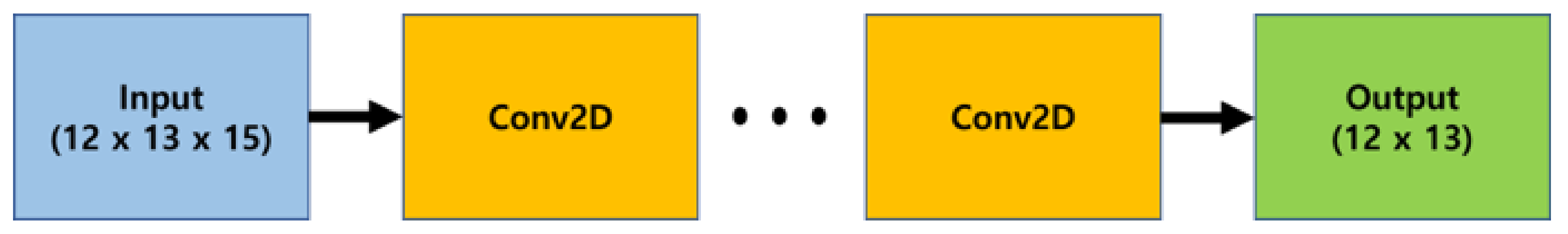
2.4.2. Model Structure

Figure 3 illustrates the structure of the model developed in this study. This experiment was conducted by configuring the hidden layers of one to three CONV2D into one to three layers. The input layer and the hidden layer are each composed of 14 features, and the output layer comprises one feature corresponding to the spatial distribution of C. polykrikoides blooms. For the weight, the bias was set to zero, and the global uniform kernel initializer was used. During training, the Adam optimizer was used, and tanh (hyperbolic tangent) was applied as the activation function of the hidden layer because it could learn the characteristics of the occurrence of C. polykrikoides blooms as a training target. In addition, in this experiment, 14 variables of the input data were normalized to optimize the training because the deviation was large, depending on the parameters of the input data.

2.4.3. Training and Test Period

Our deep learning prediction model was trained using meteorological and oceanographic input data from 2010 to 2019. The occurrence information of C. polykrikoides was also considered. The ratio of training, verification, and test data was set at 8:1:1, the training structure was one-to-one based on matching of the ocean and meteorological data on the same date as the corresponding C. polykrikoides bloom date, and the possible C. polykrikoides bloom occurrence forecasting date is the same as the future forecasting period of HYCOM and GFS. For example, if HYCOM and GFS each have a prediction result of 3 days and 10 days, respectively, the maximum predictable period in this study is 3 days.

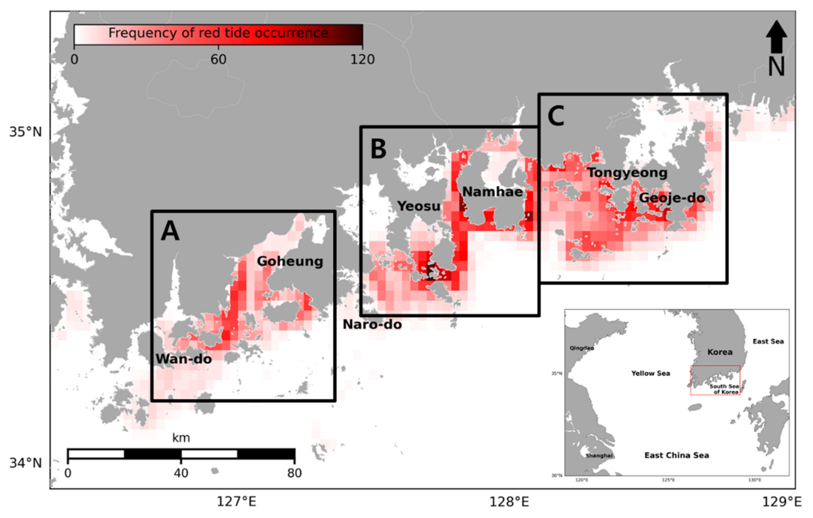
2.4.4. Model Domain and Information

In Figure 1A,B and C are all composed of a 12 × 13 grid, and the ocean and meteorological data used for model training were also interpolated to form a grid of the same size as A, B, and C. Because there are 14 marine and meteorological variables, the input layer is composed of 12 × 13 × 15 3D data, and the output layer provides 12 × 13 × 1 2D C. polykrikoides bloom information. In the case of the hidden layer, the padding is set such that the input layer and grid size are the same, and the filter size is 14 that is the same as the number of input variables.

HABs are affected by various environmental factors, not only around the location of blooming, but also those that are far from the blooming areas. This study was conducted based on the hypothesis that the impacts of environmental factors on HABs are proportional to the distance from the blooming areas; therefore, we set the kernel size to three.

2.4.5. Network Architecture

In the experiment, the dates of HAB occurrence and non-occurrence in each domain were randomly mixed. The ratios of training, verification, and testing were 80%, 10%, and 10%, respectively. The test was conducted on HAB information for 24 days that corresponds to 10% of the total period of HAB information.

3. Results

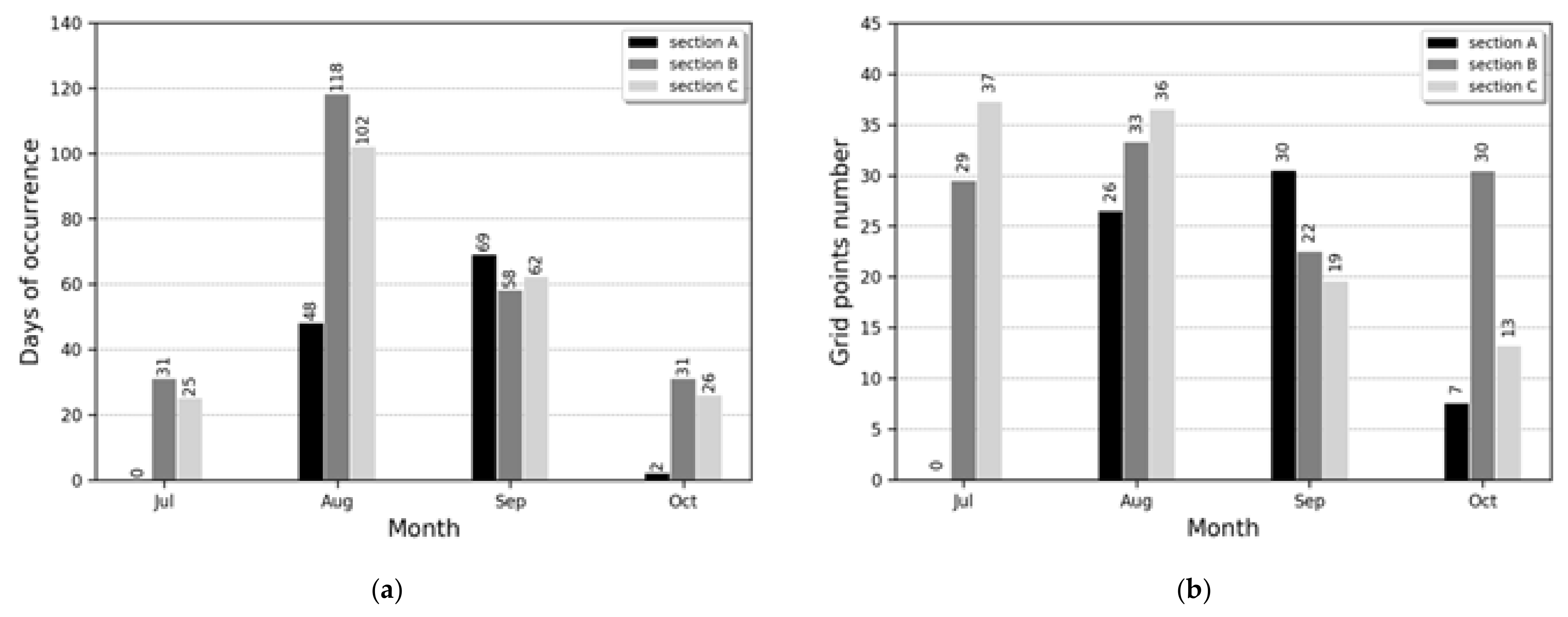
3.1. HABs Occurrence Status

In the SSK, HABs occur mainly from July to October, most frequently in August. Therefore, we simulated the HABs from July to October from 2010 to 2019. The HAB occurrence days during the analysis period was 279 days. Figure 4 shows the cumulative occurrence days of HABs per month from 2010 to 2019.

The test data (ocean, meteorology) were used along with training data (ocean, meteorology) and its label (HABs observation data) to verify the HAB occurrence prediction performance. Figure 5a shows the number of days of HAB occurrence per month for each domain. In Domain A, HABs began to occur in August, with the highest frequency (69 days) in September. Domain B and C show similar occurrence days of HABs. HABs began to occur in July, the highest frequency being (Domain B: 118 days, Domain C: 102 days) in August that gradually decreased from September due to the decrease in water temperature. Figure 5b shows the monthly HAB occurrence area (number of pixels) for each domain. Domain A showed the largest occurrence area in September that was proportional to the number of days of HABs. In Domain B, the difference in the occurrence area between months is small, indicating that the HABs in Domain B are widely distributed. Domain C had the largest distribution area in July that gradually decreased until October. Therefore, it can be confirmed that HABs actively occur in July and August in Domain B and C and decrease in September, while Domain A shows the maximum HABs in September. SSK had different spatial and temporal characteristics for each region. Accordingly, the domains were divided considering the characteristics of each area.

3.2. CONV2D Forecasting of HABs for the Three Domains

The grid size of the meteorological and ocean input variables was set as 58 × 78 at 0.5° grid resolution and interpolated accordingly. The input time was 279 days, and the total number of HAB occurrence days between 2010 and 2019 and the total number of input variables was 15, including meteorological and oceanic variables. Therefore, the number of variables in the HAB generation prediction model was 18,932,940 (= 79 × 58 × 78 × 15). The output variables corresponded to each experimental area, and the experiment considered the information regarding the presence or absence of HABs in each grid in a grid of size 12 × 13 at 0.5° grid resolution. Therefore, the number of output variables of the HAB occurrence prediction model was 43,524 (= 79 × 12 × 13). After setting each experimental group based on the aforementioned configuration, we attempted to predict the occurrence of HABs using CONV2D. The structure of the HAB occurrence prediction using CONV2D is shown in Figure 3. This model configuration results from the input data set specified in the HAB occurrence information true value as predicted daily HAB occurrence (one-to-one).

Subsequently, the experiments were conducted for different numbers of classes. In other words, one to three layers were used. As presented in

Table 3. Validation result (Average MSE and ACC) using different convolution strategies and iteration times for Domain A, B, and C.

Domain	Layer		Iterations (times)
			50	100	150	200	250	300
A	1	Loss	0.0159	0.0152	0.0144	0.0147	0.0146	0.0133
		Accuracy	0.9812	0.9811	0.9818	0.9825	0.9825	0.9837
	2	Loss	0.0157	0.0147	0.0140	0.0131	0.0129	0.0126
		Accuracy	0.9813	0.9823	0.9828	0.9844	0.9843	0.9846
	3	Loss	0.0164	0.0146	0.0146	0.0137	0.0132	0.0125
		Accuracy	0.9803	0.9818	0.9818	0.9833	0.9842	0.9852
B	1	Loss	0.0405	0.0386	0.0370	0.0352	0.0342	0.0340
		Accuracy	0.9484	0.9515	0.9541	0.9569	0.9572	0.9568
	2	Loss	0.0387	0.0347	0.0321	0.0310	0.0281	0.0298
		Accuracy	0.9505	0.9564	0.9598	0.9614	0.9661	0.9634
	3	Loss	0.0394	0.0345	0.0304	0.0286	0.0293	0.0271
		Accuracy	0.9498	0.9566	0.9628	0.9649	0.9628	0.9669
C	1	Loss	0.0351	0.0330	0.0310	0.0306	0.0295	0.0288
		Accuracy	0.9577	0.9600	0.9629	0.9628	0.9650	0.9660
	2	Loss	0.0341	0.0313	0.0284	0.0267	0.0256	0.0252
		Accuracy	0.9596	0.9624	0.9662	0.9685	0.9713	0.9707
	3	Loss	0.0352	0.0313	0.0299	0.0264	0.0254	0.0250
		Accuracy	0.9582	0.9634	0.9657	0.9686	0.9716	0.9716

, all the three weighted convolutional LSTM layers demonstrated the best performance in Domain A, B, and C. It can be seen that as the number of layers decreases, the result is equal or lower. Therefore, 3 weighted convolutional layers and 300 training times were considered optimal for the HAB occurrence prediction model. The experiment was conducted for the period set as the test experiment. The bold characters in Table 3 indicate the best performance: the smallest RMSE and the largest ACC.

In terms of the number of CONV2D layers, the accuracy with 300 training times for a single stack of Domains A, B, and C was 96.88%, and the accuracy with 300 training times for three stacks was 97.46%, demonstrating a 0.58% improvement. In terms of the number of training times in the three-stack CONV2D layer, the convergence of training and verification loss was not observed for less than 200 training times. It appeared to be a less stable training model when the training was performed at least 300 times. Therefore, a stable training model was obtained, and prediction results showing an improved accuracy were obtained.

Table 4. Average test result (pixel accuracy, mean accuracy, mean IU, frequency weighted IU) of Domain A, B, and C.

Domain	Pixel Accuracy	Mean Accuracy	Mean IU	Frequency Weighted IU
A	97.78	88.57	83.59	96.63
B	94.61	86.19	79.72	91.95
C	96.98	80.06	74.63	95.31
Total	96.46	84.94	79.31	94.63

presents the performances of the proposed model in Domain A, B, and C, as well as the overall results. The evaluation metrics are the pixel accuracy (PA), mean accuracy (MA), mean IU (mIU), and frequency weighted IU fwIU). The average pixel accuracy is 96.46%, while the mean accuracy is 84.94%. The mean IU and frequency weighted IU are 79.31% and 94.63%, respectively.

Overall, the proposed model realized a high accuracy for all the domains. Domain A showed the best precision for all the metrics. In Domain B, PA and fwIU were lower than the average values, while MA and mIU in Domain C were lower than the average values.

4. Summary and Discussion

In this study, we combined spatial and temporal information to predict the occurrence of HAB. The SSK region, where HABs frequently occurs, consists of many inner bays owing to its complex ria coast. Because each inner bay has its own maritime characteristics, we established prediction domains for three regions.

The optimal model setup was achieved by conducting various experiments using 1–3 convolutional Long-Short Term Memory(convLSTM) layers and 50–300 iterative pieces of training for each domain. The best deep learning network setup was obtained from the experiments using 3 convLSTM layers and 300 iterative pieces of training. Because the complexity of the deep learning model is extremely high, it is necessary to establish several layers and a corresponding iterative training number. Recently, deep learning techniques have been used for performing predictions in various fields; however, owing to the limitations of the memory capacity of the mounted GPGPU (General-Purpose Computing on Graphics Processing Units), it is difficult to address the complexity of the multi-dimensional models used in this study. GPGPU performance can be improved in the future using higher resolution meteorological and oceanic input data that are available, and consequently, the prediction accuracy is expected to increase further.

The performance metrics corresponding to the domains showed high efficiency. However, in all the domains, the results were over-predicted; this is also associated with the results where the accuracy was higher than the IU. For the performance evaluation metrics, accuracy represents only the percentage of successful predictions of red tide occurrences, and predictions of non-occurrence are not considered, whereas IU considers both occurrence and non-occurrence. Furthermore, fwIU and PA show higher values than mIU and MA that is in accordance with the definition of metrics. MA and mIU represent the straightforward average of the occurrence and non-occurrence predicted hit rates, but PA and fwIU increase the proportion of the larger class between occurrence and nonoccurrence. Consequently, PA and fwIU can be more useful when HABs are distributed in most regions.

The characteristics of HABs differed for each domain, with frequent HABs in July and August in Domain A, as the past data used for training includes cases in which HABs occurred in the western SSK in 2013 and 2014 due to abnormally high water temperatures [30]. It is also considered that the accuracy of Domain B and C was lower than that of domain A is related to the characteristics of the ocean currents in the SSK. The Tsushima Warm Current inflow, which plays a key role in the circulation of the SSK, flows from the west to the east. Consequently, in Domain B and C, HAB occurrences are not only induced by environmental factors, but also by easterly flowing ocean currents.

Overall, the deep learning model proposed in this study is considered to be useful for predicting HAB occurrence off the southern coast of Korea. A more complex and accurate prediction method combining spatial and temporal information can be applied to various marine disasters based on the improvement of deep learning models and computational equipment performances in the future.

The deep learning method can be applied widely and generally to various problems. We expect our proposed method can be modified and applied to other environment predictions, such as hypoxic state and shellfish toxin which are closely related to oceanic and atmospheric states.

References

1. Kim, H.G. Harmful Algal Blooms in the Sea; Dasom Publishing, Co.: Seoul, Korea, 2015; p. 467. [Google Scholar]
2. Kang, Y.S.; Kim, H.G.; Lim, W.E.; Lee, C.K. An unusual coastal environment and Cochlodinium polykrikoides blooms in 1995 in the South Sea of Korea. J. Korean Soc. Oceanogr. 2002, 37, 212–223. [Google Scholar]
3. Suh, Y.S.; Jang, L.H.; Lee, N.K.; Ishizaka, J. Feasibility of red tide detection around Korea waters using satellite remote sensing. Fish. Aquat. Sci. 2004, 7, 148–162. [Google Scholar] [CrossRef] [Green Version]
4. Gómez, F.; Richlen, M.L.; Anderson, D.M. Molecular characterization and morphology of Cochlodinium strangulatum, the type species of Cochlodinium, and Margalefidinium gen. nov. for C. polykrikoides and allied species (Gymnodiniales, Dinophyceae). Harmful Algae 2017, 63, 32–44. [Google Scholar] [CrossRef] [PubMed]
5. Lee, S.G.; Kim, H.G.; Bae, H.M.; Kang, Y.S.; Jeong, C.S.; Lee, C.K.; Kim, S.Y.; Kim, C.S.; Lim, W.A.; Cho, U.S. Handbook of Harmful Marine Algal Blooms in Korean Waters; National Fisheries Research and Development Institute: Gangwon-do, Korea, 2002; p. 172. [Google Scholar]
6. Stumpf, R.P.; Arnone, R.A.; Gould, R.W.; Martinolich, P.M.; Ransibrahmankul, V. A partially coupled ocean-atmosphere model for retrieval of water-leaving radiance from SeaWiFS in coastal waters. SeaWiFS Postlaunch Tech. Rep. Ser. 2003, 22, 51–59. [Google Scholar]
7. Ahn, Y.H.; Shanmugam, P. Detecting the red tide algal blooms from satellite ocean color observations in optical complex Northeast-Asia coastal waters. Remote Sens. Environ. 2006, 103, 419–437. [Google Scholar] [CrossRef]
8. Son, Y.B.; Ishizaka, J.; Jeong, J.C.; Kim, H.C.; Lee, T. Cochlodinium polykrikoides red tide detection in the south sea of Korea using spectral classification of MODIS data. Ocean Sci. J. 2011, 46, 239–263. [Google Scholar] [CrossRef]
9. Lee, S.M.; Lee, D.H. Improved prediction of harmful algal blooms in four Major South Korea’s Rivers using deep learning models. Int. J. Environ. Res. Public Health 2018, 15, 1322. [Google Scholar] [CrossRef] [Green Version]
10. Zhang, F.; Wang, Y.; Cao, M.; Sun, X.; Du, Z.; Liu, R.; Ye, X. Deep-learning-based approach for prediction of algal blooms. Sustainability 2016, 8, 1060. [Google Scholar] [CrossRef] [Green Version]
11. Daghighi, A. Harmful Algae Bloom Prediction Model for Western Lake Erie Using Stepwise Multiple Regression and Genetic Programming. Bachelor’s Thesis, University of Tehran, Tehran, Iran, 19 February 2015. [Google Scholar] [CrossRef]
12. Derot, J.; Yajima, H.; Jacquet, S. Advances in forecasting harmful algal blooms using machine learning models: A case study with Planktothrix rubescens in Lake Geneva. Harmful Algae 2020, 99, 101906. [Google Scholar] [CrossRef]
13. Bak, S.H.; Kim, H.M.; Kim, B.K.; Hwang, D.H.; Unuzaya, E.; Yoon, H.J. Study on detection technique for Cochlodinium polykrikoides red tide using logistic regression model and decision tree model. J. Korea Inst. Electron. Commun. Sci. 2018, 13, 777–786. [Google Scholar] [CrossRef]
14. Bak, S.H.; Jeong, M.J.; Hwang, D.H.; Enkhjargal, U.; Yoon, H.J. Study on Cochlodinium polykrikoides red tide prediction using deep neural network under imbalanced data. J. Korea Inst. Electron. Commun. Sci. 2019, 14, 1161–1170. [Google Scholar] [CrossRef]
15. Shin, J.; Kim, S.M.; Son, Y.B.; Kim, K.; Ryu, J.H. Early prediction of Margalefidinium polykrikoides bloom using a LSTM neural network model in the south sea of Korea. J. Coast. Res. 2019, 90, 236–242. [Google Scholar] [CrossRef]
16. Kim, S.M.; Shin, J.; Baek, S.; Ryu, J.H. U-Net convolutional neural network model for deep red tide learning using GOCI. J. Coast. Res. 2019, 90, 302–309. [Google Scholar] [CrossRef]
17. Shin, J.; Min, J.E.; Ryu, J.H. A study on red tide surveillance system around the Korean coastal waters using GOCI. Korean J. Remote Sens. 2017, 33, 213–230. [Google Scholar] [CrossRef]
18. Lee, M.O.; Lee, S.H.; Kim, P.J.; Kim, B.K. Characteristics of water masses and its distributions in the southern coastal waters of Korea in summer. J. Korean Soc. Mar. Environ. Energy 2018, 21, 76–96. [Google Scholar] [CrossRef]
19. Gobler, C.J.; Berry, D.L.; Anderson, O.R.; Burson, A.; Koch, F.; Rodgers, B.S.; Moore, L.K.; Goleski, J.A.; Allam, B.; Bowser, P.; et al. Characterization, dynamics, and ecological impacts of harmful Cochlodinium polykrikoides blooms on eastern Long Island, NY, USA. Harmful Algae 2008, 7, 293–307. [Google Scholar] [CrossRef]
20. Kudela, R.M.; Ryan, J.P.; Blakely, M.D.; Lane, J.Q.; Peterson, T.D. Linking the physiology and ecology of Cochlodinium to better understand harmful algal bloom events: A comparative approach. Harmful Algae 2008, 7, 278–292. [Google Scholar] [CrossRef]
21. Mulholland, M.R.; Morse, R.E.; Boneillo, G.E.; Bernhardt, P.W.; Filippino, K.C.; Procise, L.A.; Blanco-Garcia, J.L.; Marshall, H.G.; Egerton, T.A.; Hunley, W.S.; et al. Understanding causes and impacts of the dinoflagellate, Cochlodinium polykrikoides, blooms in the Chesapeake Bay. Estuar. Coast. 2009, 32, 734–747. [Google Scholar] [CrossRef]
22. Fatemi, S.M.R.; Nabavi, S.M.B.; Vosoghi, G.; Fallahi, M.; Mohammadi, M. The relation between environmental parameters of Hormuzgan coastline in Persian Gulf and occurrence of the first harmful algal bloom of Cochlodinium polykrikoides (Gymnodiniaceae). Iran. J. Fish. Sci. 2012, 11, 475–489. [Google Scholar]
23. Kudela, R.M.; Gobler, C.J. Harmful dinoflagellate blooms caused by Cochlodinium sp.: Global expansion and ecological strategies facilitating bloom formation. Harmful Algae 2012, 14, 71–86. [Google Scholar] [CrossRef]
24. Al-Azri, A.R.; Piontkovski, S.A.; Al-Hashimi, K.A.; Goes, J.I.; Gomes, H.R.; Glibert, P.M. Mesoscale and nutrient conditions associated with the massive 2008 Cochlodinium polykrikoides bloom in the Sea of Oman/Arabian Gulf. Estuar. Coast. 2013, 37, 325–338. [Google Scholar] [CrossRef] [Green Version]
25. Zuo, X.; Zhou, X.; Guo, D.; Li, S.; Liu, S.; Xu, C. Ocean Temperature Prediction Based on Stereo Spatial and Temporal 4-D Convolution Model. IEEE Geosci. Remote Sens. Lett. 2021, 19, 1003405. [Google Scholar] [CrossRef]
26. Choi, H.; Park, M.; Son, G.; Jeong, J.; Park, J.; Mo, K.; Kang, P. Real-time significant wave height estimation from raw ocean images based on 2D and 3D deep neural networks. Ocean. Eng. 2020, 201, 107129. [Google Scholar] [CrossRef]
27. Segal-Rozenhaimer, M.; Li, A.; Das, K.; Chirayath, V. Cloud detection algorithm for multi-modal satellite imagery using convolutional neural-networks (CNN). Remote Sens. Environ. 2020, 237, 111446. [Google Scholar] [CrossRef]
28. Schmid, M.S.; Cowen, R.K.; Robinson, K.; Luo, J.Y.; Briseño-Avena, C.; Sponaugle, S. Prey and predator overlap at the edge of a mesoscale eddy: Fine-scale, in-situ distributions to inform our understanding of oceanographic processes. Sci. Rep. 2020, 10, 921. [Google Scholar] [CrossRef] [Green Version]
29. Lecun, Y.; Bottou, L.; Bengio, Y.; Haffner, P. Gradient-based learning applied to document recognition. Proc. IEEE 1998, 86, 2279–2324. [Google Scholar] [CrossRef] [Green Version]
30. Jeong, Y.; Kim, M.; Cho, A.; Yoon, S.; Park, Y.; Son, M.; Choi, H.; Cho, H. The western waters of the South Sea in 2013–2014, characteristics of Cochlodinium polykrikoides. Proc. Korean Soc. Mar. Environ. Energy 2016, 11, 162–163. [Google Scholar]
Figure 1. Cumulative occurrence days of C. polykrikoides per grid from 2010 to 2019 in the SSK based on the observed data provided by NIFS (A, B, and C indicate the C. polykrikoides forecasting experiment area).
Jmse 10 00031 g001
Figure 2. A convolutional neural network sequence to classify ocean data.
Jmse 10 00031 g002
Figure 3. Network structure of the HAB prediction model.
Jmse 10 00031 g003
Figure 4. Cumulative days of HABs per month from 2010 to 2019 at the SSK.
Jmse 10 00031 g004
Figure 5. Monthly HABs occurrence days (a) and areas (b) by domains.
Jmse 10 00031 g005