A Hybrid RF–XGBoost Model for Soil Temperature Prediction in Solar Greenhouses

Abstract

Solar greenhouses are indispensable infrastructure for winter vegetable production in high-latitude regions, maintaining favorable growing conditions without auxiliary heating through superior thermal insulation and solar radiation capture. However, extreme meteorological events disrupt this equilibrium, and soil temperature prediction remains challenging due to thermal hysteresis—time-lagged responses to environmental drivers that threaten crop viability during pre-dawn periods. Existing studies focus on air temperature or short-term horizons (3–6 h), leaving the critical 12 h prediction window inadequately addressed. This study develops a hybrid machine learning framework for 12 h soil temperature prediction in a solar greenhouse. High-resolution data were collected using soil temperature sensors at 200 mm depth (tomato root zone) during the winter growing season. Five algorithms were evaluated: RF and XGBoost (Bagging/Boosting for trend/residual capture), LSTM and GRU (temporal memory), and a novel RF-XGBoost hybrid with two-stage residual correction. The hybrid model achieved R² = 0.9927, improving standalone RF (R² = 0.9883) by 0.45% with MSE, RMSE, MAE reductions of 18.1%, 9.6%, 13.9%. Maximum 12 h error was 2.52 °C versus 3.12–4.60 °C for standalone models. The 12 h horizon enables preemptive heating activation, mitigating frost risk while avoiding unnecessary energy expenditure.

1. Introduction

Solar greenhouses are indispensable infrastructure for winter vegetable production in high-latitude regions, particularly in Northern China [1]. These structures maintain favorable growing conditions without auxiliary heating by leveraging superior thermal insulation and heat storage capacity of their north walls, combined with optimized transparent front roof designs that maximize solar radiation capture [2]. However, extreme meteorological events—such as sudden cold waves, heavy snowfall, or prolonged overcast periods—often disrupt this equilibrium. Under such conditions, the internal microclimate, particularly the soil temperature, exhibits significant recovery delays due to the thermal inertia and hysteresis inherent in the soil–plant–atmosphere system [3,4].

The strategic emphasis on soil temperature prediction, as opposed to ambient air temperature, is dictated by three critical factors. Physically, soil temperature is a more sensitive determinant of crop health than air temperature, directly modulating root activity, nutrient uptake, and rhizosphere microbial dynamics [5,6]. Economically, root-zone heating is more energy-efficient than space heating, making precise soil temperature forecasting a prerequisite for low-carbon precision agriculture [7]. Structurally, the soil’s high thermal mass provides a buffered, predictable metric for long-term stability, offering a more robust baseline for cold-stress mitigation strategies [8].

Maintaining soil temperature above critical physiological thresholds (typically 12–15 °C for solanaceous crops) is essential to prevent irreversible yield loss [9]. In this context, establishing a 12 h prediction horizon is vital for proactive greenhouse climate control. Unlike ultra-short-term forecasts (3–6 h), which offer limited response time, or multi-day models, which suffer from compounded stochastic errors, a 12 h window aligns with the fundamental diurnal cycle of greenhouse operations [10]. It provides the necessary lead time to implement preemptive thermal management—such as early deployment of thermal blankets or the modulation of auxiliary heating—ensuring stability during the high-risk pre-dawn period.

Despite its importance, the accurate estimation of soil temperature remains a non-trivial challenge due to the nonlinear coupling of hydrothermal processes within the soil–plant–atmosphere continuum [11]. Existing methodologies fall into three categories: (1) in situ measurement techniques, (2) computational fluid dynamics (CFD) simulations, and (3) machine learning (ML)-based predictive models. In situ methods, including thermistor sensors and platinum resistance thermometers, provide high-precision data but suffer from sparse spatial coverage, labor-intensive maintenance, and poor scalability for real-time decision-making [12]. CFD simulations offer detailed spatiotemporal thermal dynamics by solving energy balance equations coupled with radiative transfer models, yet they require extensive parameter calibration, predefined boundary conditions, and computational times incompatible with operational greenhouse management [13]. These limitations motivate the exploration of data-driven ML approaches that can capture complex nonlinear relationships without explicit physical parameterization.

Machine learning methods for greenhouse soil temperature prediction can be classified into single models and ensemble models. Single models include both tree-based algorithms (Random Forest, RF; XGBoost) and sequential deep learning architectures (Long Short-Term Memory, LSTM; Gated Recurrent Unit, GRU). The physical rationale for this selection is grounded in the distinct temporal characteristics of soil thermal dynamics: (i) thermal hysteresis, where soil temperature responds to air temperature and solar radiation with a time lag that depends on soil depth and moisture content [14]; (ii) nonlinear interactions between indoor/outdoor temperatures, solar radiation, and soil properties [15]; and (iii) diurnal and seasonal periodicities superimposed on weather-driven anomalies [16]. Tree-based ensembles (RF, XGBoost) excel at capturing static nonlinear feature interactions through recursive partitioning, while sequential models (LSTM, GRU) are specifically designed to model temporal dependencies via gating mechanisms that mitigate vanishing gradients in long sequences [17,18]. This complementary functionality motivates their comparative evaluation for soil temperature forecasting.

Recent studies have demonstrated promising results for both approaches. Myeni et al. [19] reported RF achieved Nash–Sutcliffe efficiency of 0.87–0.95 for multi-depth soil temperature estimation, while Kucukerdem [20,21] obtained R² > 0.99 using XGBoost for root-zone temperature prediction. For sequential modeling, Liu et al. [22] showed GRU outperformed LSTM with 12.3–27.5% RMSE reduction across 15–1440 min horizons. Li et al. [23] further advanced sequential modeling by integrating multi-head attention mechanisms with LSTM, achieving R² = 0.96 for 30 min soil temperature forecasts; however, this architecture remains a single-model framework whose performance degrades to R² = 0.89 at 8 h horizons and exhibits pronounced volatility under fluctuating thermal conditions. Despite these advances, single models exhibit fundamental limitations: tree-based methods lack explicit temporal memory, rendering them insensitive to thermal lag dynamics [24], whereas deep learning models require large training datasets and are prone to overfitting with noisy agricultural sensor data [25]. Furthermore, static prediction frameworks cannot dynamically correct accumulated errors under drifting environmental conditions, such as the abrupt temperature declines observed during extreme weather events [26].

Ensemble strategies that integrate complementary model strengths offer a pathway to overcome these limitations. Wang et al. [27] proposed a ReSSA-iTransformer hybrid achieving R² > 94.83% across 3–48 h horizons, though this approach relies on complex signal decomposition without explicit physical constraints. Critically, no existing study has systematically evaluated the integration of tree-based feature extraction with gradient-boosted residual correction for greenhouse soil temperature prediction, nor have they implemented rolling prediction frameworks that dynamically adjust forecasts based on accumulated environmental history. These gaps are particularly acute for solar greenhouses in extreme cold climates, where thermal inertia effects are amplified and prediction errors directly impact heating energy costs and crop safety.

Based on these considerations, we hypothesize that: (1) a two-stage hybrid model combining RF (for dominant nonlinear trend capture) and XGBoost (for residual error correction) will outperform standalone models by disentangling stable thermal patterns from hysteresis-induced fluctuations; (2) a 48 h historical sequence input with dual-periodic feature encoding (hour-of-day, day-of-year) will enable accurate 12 h rolling predictions that respect the physical constraints of soil thermal dynamics; and (3) this framework will maintain robust performance under extreme weather stress (cold snaps, consecutive overcast days) where single models exhibit significant degradation.

To test these hypotheses, this study establishes a soil temperature prediction framework using three months of high-resolution monitoring data (7681 timesteps, 15 min intervals) from a solar greenhouse at Shenyang city. The specific objectives are: (1) to quantify cross-correlations between environmental variables and soil temperature to validate the temporal modeling approach; (2) to develop and validate a RF-XGBoost two-stage hybrid model with explicit residual correction mechanisms; (3) to implement a rolling 12 h prediction framework with 48 h historical memory and dual-periodic feature engineering; and (4) to evaluate model reliability under documented extreme weather events (December cold snap: −13 °C average outdoor temperature; December consecutive overcast: solar radiation < 40 W/m²). This research advances beyond existing methodologies by explicitly embedding soil physical constraints (thermal inertia, hysteresis, periodicity) into a computationally efficient ML architecture suitable for real-time greenhouse climate control.

2. Materials and Methods

2.1. Greenhouse Facilities and Experimental Setup

2.1.1. Greenhouse Structure and Specifications

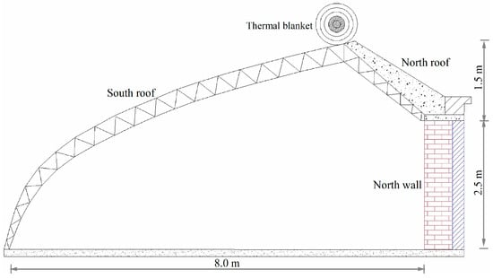
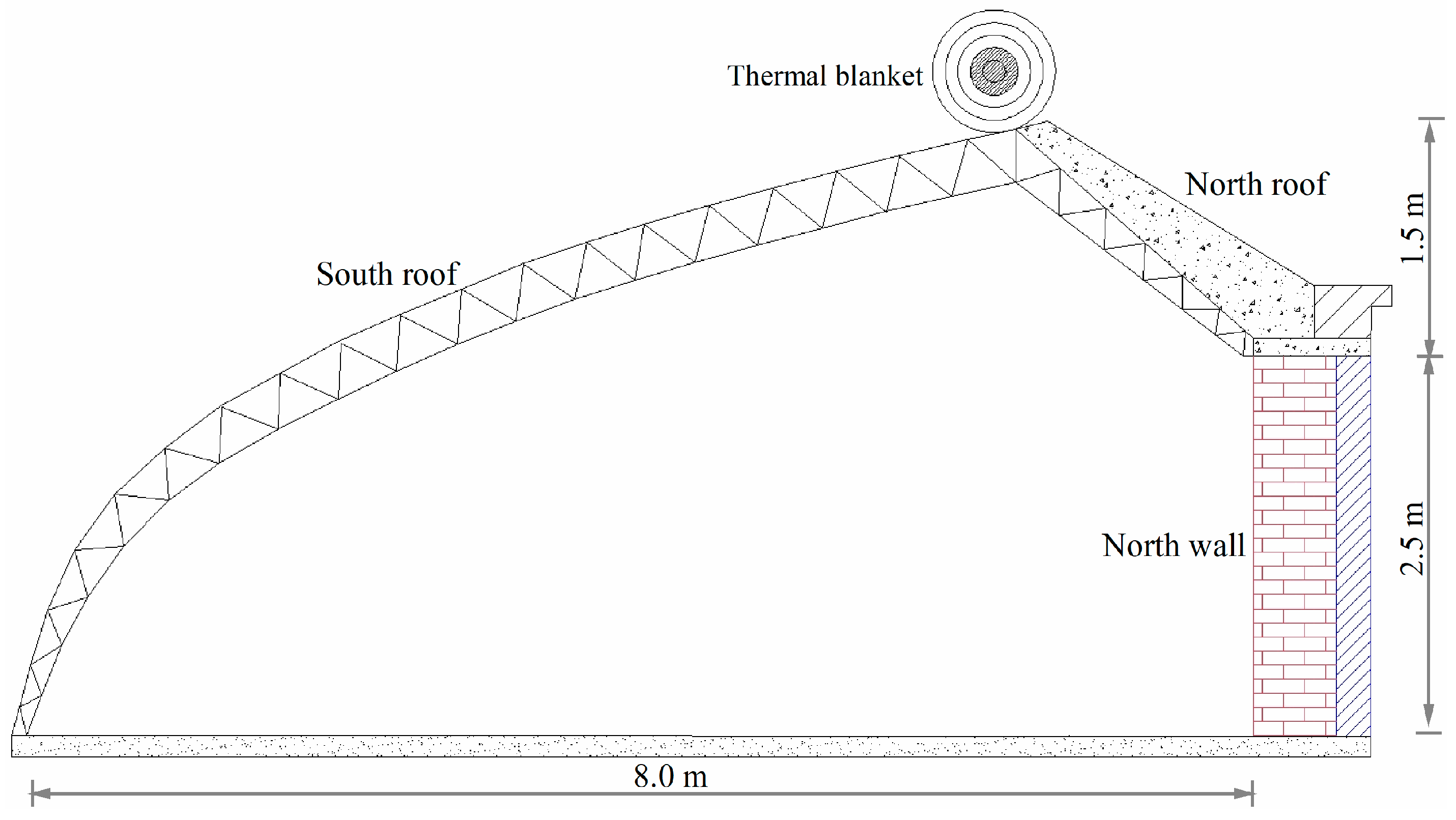
The experiment was conducted in a solar greenhouse located at Shenyang Agricultural University (41°48′ N, 123°25′ E), a representative facility for solar greenhouse vegetable production in Northeast China (Figure 1). The greenhouse featured an east–west orientation with the following structural specifications: total length of 60 m, span width of 8.0 m, ridge height of 4.0 m, and north wall height of 2.5 m. The north wall was constructed with a composite thermal insulation structure comprising a 370 mm thick hollow clay brick layer and a 110 mm thick polystyrene foam board insulation layer. The south roof was covered with 0.15 mm thick polyolefin (PO) agricultural film, and a quilted thermal blanket was deployed on the south roof from late afternoon (15:30) to early morning (08:30) to minimize heat loss during periods of low solar radiation.

Figure 1. Schematic diagram of the solar greenhouse.

During the experimental period, the greenhouse operated under typical commercial cultivation conditions, with tomato plants grown throughout the study. The crop was arranged in a north–south (N–S) row orientation with a wide–narrow row configuration, including a large row spacing of approximately 0.8 m, a small row spacing of 0.4 m, and a plant spacing of 0.4 m, consistent with common greenhouse tomato production practices in northern China.

The soil surface was continuously covered with plastic mulch, and irrigation was applied using a drip irrigation system installed beneath the mulch (mulched drip irrigation). Drip lines were arranged with one line per crop row, with emitters positioned near the root zone of each plant, a spacing of 0.4 m, and a nominal discharge rate of 1.6 L h⁻¹ under an operating pressure of 0.3 MPa. This cultivation practice is widely used to reduce soil evaporation, maintain relatively stable soil moisture, and regulate soil thermal conditions.

2.1.2. Monitoring Systems and Sensor Specifications

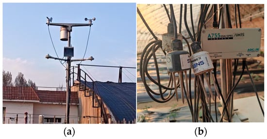
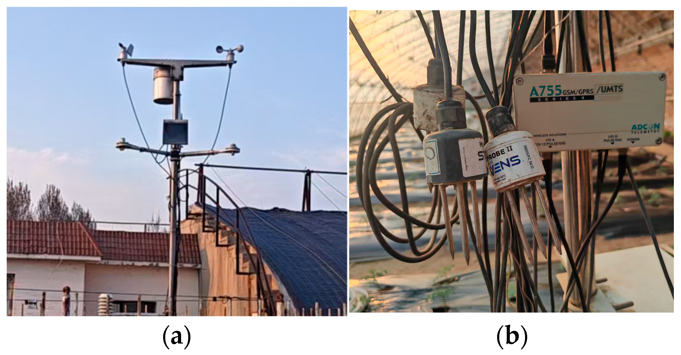
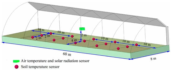
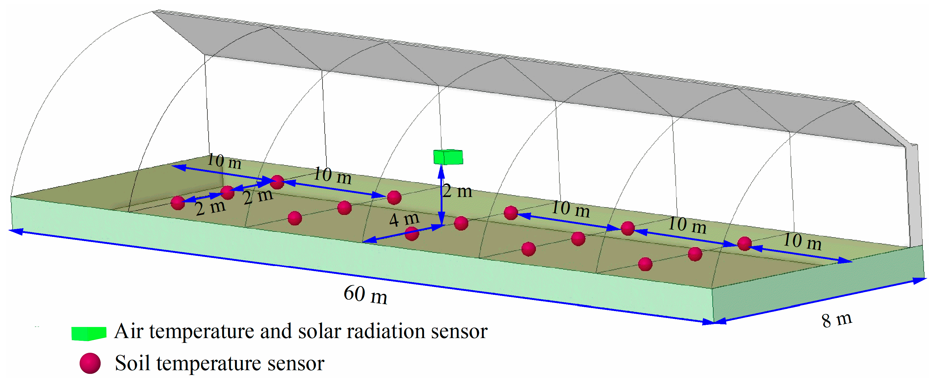
Environmental parameters were monitored using an integrated sensor network comprising meteorological and soil temperature measurement systems. The monitoring devices, including the outdoor meteorological station and the indoor data acquisition system, are presented in Figure 2, while the spatial arrangement of sensors is illustrated in Figure 3.

Figure 2. (a) Meteorological station and (b) data acquisition system with soil temperature sensors.

Figure 3. Spatial arrangement of environmental and soil temperature sensors in the greenhouse.

Outdoor meteorological conditions were monitored using an ADCON A753 meteorological station (Adcon Telemetry GmbH, Klosterneuburg, Austria), which continuously recorded outdoor air temperature and global solar radiation. The air temperature sensor had a measurement range of −40 to 60 °C with an accuracy of ±0.2 °C at 20 °C. The global solar radiation sensor had a measurement range of 0–2000 W m⁻², with a temperature response within ±3% (−10–40 °C), annual drift less than 1%, nonlinearity < ±1% (100–1000 W m⁻²), and tilt response < ±2% (0–90°, at 1000 W m⁻²).

Indoor environmental variables were monitored using an ADCON A755 GSM/GPRS data acquisition system (Adcon Telemetry GmbH, Klosterneuburg, Austria), which collected and transmitted data from sensors installed inside the greenhouse. The system continuously recorded greenhouse air temperature and soil temperature. The indoor air temperature sensor had the same measurement range and accuracy as the outdoor temperature sensor (−40 to 60 °C, accuracy ±0.2 °C at 20 °C). Soil temperature was measured using soil temperature probes connected to the A755 GSM/GPRS system, with a measurement range of −20 to 60 °C and an accuracy of ±0.1 °C.

Indoor air temperature and solar radiation sensors were installed at the central cross-section of the greenhouse (i.e., 30 m from the gable end), positioned 4 m from the south-facing front wall and at a height of 2 m above the ground, as illustrated in Figure 3.

Soil temperature sensors were arranged to capture the spatial variability of soil thermal conditions. Along the greenhouse span direction, sensors were evenly distributed with a spacing of 2 m. Along the longitudinal (east–west) direction, sensors were arranged in five columns with an interval of 10 m between adjacent columns, as shown in Figure 3. All sensors were installed at a depth of 200 mm, corresponding to the primary root-zone depth (150–250 mm) for tomato cultivation in this region [28]. This configuration enabled effective monitoring of both longitudinal and transverse soil temperature gradients within the greenhouse. Sensors were installed horizontally using a soil auger to minimize soil disturbance, and thermal paste was applied to ensure good thermal contact between the sensor probe and the surrounding soil. All environmental data were recorded at 15 min intervals through the monitoring system.

2.1.3. Sensor Calibration and Data Quality Assurance

All soil temperature sensors underwent comprehensive calibration and validation procedures to ensure measurement reliability. Prior to field deployment, sensors were calibrated against a reference PT100 thermometer (accuracy: ±0.01 °C) in a circulating water bath across the operational range of 0–40 °C at 5 °C intervals, and those exhibiting deviations exceeding ±0.1 °C were excluded from the study (3 of 15 sensors). Field validation was conducted by installing two additional sensors at 200 mm depth with data logged by an independent Campbell CR1000 datalogger; comparison of 30-day concurrent measurements yielded an RMSE of 0.08 °C and R² > 0.99, confirming the reliability of the ADCON system. To maintain long-term accuracy, sensors were extracted and recalibrated biannually at the beginning and end of each growing season. Data quality assurance incorporated automated range tests (eliminating values outside −10 to +50 °C), spike detection algorithms (flagging ±3 °C changes within 15 min intervals for manual review), and monthly physical inspections to verify soil-sensor contact integrity.

2.1.4. Experimental Period and Data Selection

Measurements were conducted during two winter–spring growing seasons: 2017–2018 and 2018–2019. The 2017–2018 season was used for system adjustment, stable operation, and preliminary validation of the monitoring methodology.

For model development and analysis, data from the 2018–2019 winter production period (December 2018 to February 2019) were selected. This dataset was chosen due to its high data completeness (less than 2% missing data), stable monitoring performance, and consistent environmental and crop management conditions throughout the entire season.

The selected dataset consists of continuous time-series measurements covering December 2018, January 2019, and February 2019. Using a complete and uninterrupted dataset enables the model to capture the temporal dynamics of soil temperature under varying environmental conditions, including cold waves, overcast periods, and extreme low-temperature events, thereby improving the robustness of model evaluation.

2.2. Machine Learning Algorithms

To achieve high-precision prediction of soil temperature in solar greenhouses, this study systematically evaluates the predictive performance of two machine learning models (Random Forest and XGBoost) and two deep learning models (LSTM and GRU). These models were selected due to their complementary strengths in capturing nonlinear relationships and temporal dependencies in environmental data.

Indoor air temperature, outdoor air temperature, and solar radiation intensity were used as input features, while the measured soil temperature was taken as the target variable. Based on the performance of the individual models, an ensemble learning strategy was further developed to improve prediction accuracy by integrating the advantages of different algorithms.

The overall modeling framework consists of standalone model evaluation followed by hybrid model development, aiming to construct a robust and accurate soil temperature prediction approach for solar greenhouse environments.

2.3. Candidate Machine Learning Models

2.3.1. Long Short-Term Memory (LSTM) Recurrent Neural Network

To address the pronounced thermal hysteresis and non-stationary periodic fluctuations characteristic of soil temperature dynamics in solar greenhouses, this study employs LSTM networks for sequential prediction modeling. The gating mechanism (input, forget, and output gates) adaptively regulates the retention and discard of historical information, effectively mitigating the vanishing gradient problem inherent in conventional recurrent neural network when processing extended soil temperature sequences. This architecture enables the capture of implicit thermodynamic patterns within 48 h historical sequences that exert long-term influences on soil temperature predictions over 12 h horizons.

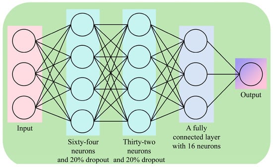
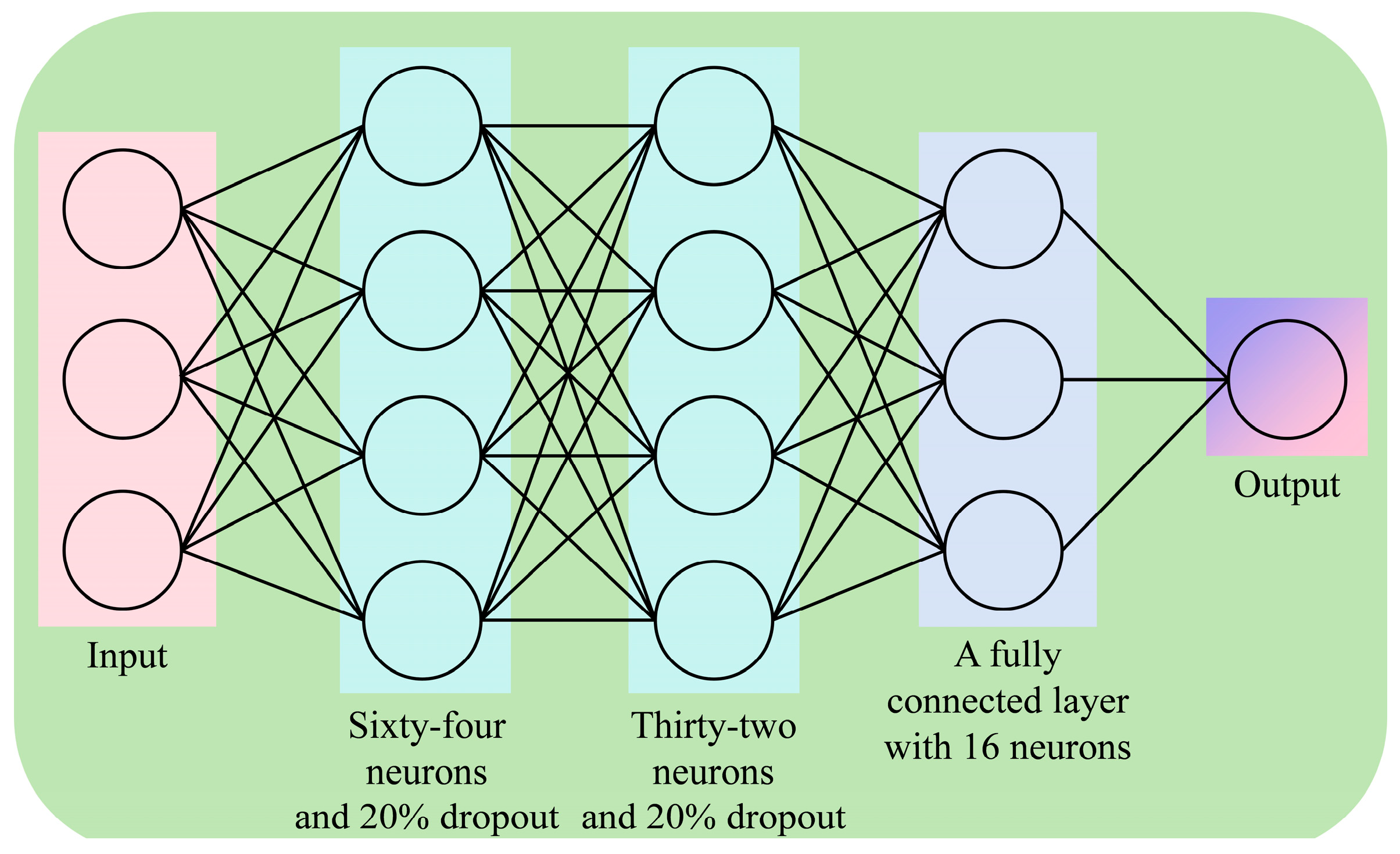
To prevent temporal data leakage in greenhouse environmental datasets, a time-sequential partitioning strategy was implemented for training and test set division. The network architecture adopts a two-layer stacked configuration: the first LSTM layer comprises 64 hidden units with return sequences enabled to extract deep temporal features (e.g., diurnal cumulative effects of soil thermal inertia); the second LSTM layer reduces to 32 hidden units to generate high-order sequence representations. Both layers incorporate 20% dropout regularization to suppress overfitting induced by sensor noise and extreme weather anomalies prevalent in greenhouse environments. Subsequently, a fully connected layer with 16 neurons applies nonlinear transformation, with the final output layer generating soil temperature predictions (Figure 4). This hierarchically decreasing neuron configuration facilitates progressive abstraction from raw environmental parameters (indoor/outdoor air temperature, solar radiation) to soil thermal state responses.

Figure 4. Neural network diagram for LSTM-based soli temperature prediction.

2.3.2. Gated Recurrent Unit (GRU)

GRU serves as a lightweight variant of LSTM, reducing parameter count through consolidated gating mechanisms (update and reset gates) while maintaining sequence modeling capabilities and enhancing training efficiency. Considering the potential real-time prediction requirements for solar greenhouse soil temperature forecasting, this study adopts GRU as a comparative architecture. Strict experimental parity is maintained by preserving identical layer numbers, hidden unit configurations (64 units in the first layer and 32 units in the second layer), dropout rates (20%), and fully connected layer specifications as the LSTM model, with sole replacement of the recurrent unit type. This design ensures rigorous evaluation of differential impacts between distinct gating mechanisms on prediction accuracy for soil thermal hysteresis.

2.3.3. Extreme Gradient Boosting (XGBoost)

To address the complex nonlinear coupling relationships between soil temperature and air temperature/solar radiation, this study implements XGBoost within a rolling prediction framework. The algorithm sequentially constructs decision trees via gradient boosting, with each new tree specifically fitting residuals from preceding ensemble models to iteratively reduce prediction bias. This characteristic proves particularly suitable for capturing nonlinear soil temperature responses to abrupt meteorological perturbations (e.g., cold snaps, consecutive overcast days) in greenhouse environments.

Given the thermal inertia properties of soil, the model input window is configured as 192 timesteps (48 h × 15 min sampling intervals), encompassing two complete diurnal thermal cycles. During prediction, the model first generates soil temperature estimates for the subsequent timestep (15 min ahead) based on the historical window, then appends this predicted value as the latest feature to the sequence terminus while eliminating the earliest timestep to maintain fixed window length. This process iterates 48 times (48 fifteen-minute intervals spanning 12 h), achieving continuous 12 h ahead forecasting. This “predict-feedback-repredict” rolling mechanism effectively simulates dynamic evolution of the soil thermal system under sustained environmental forcing. Core hyperparameter configurations are detailed in Table 1.

Table 1. Core parameters of XGBoost model.

Parameter	Value	Rationale
n_estimators	150	Balancing nonlinear complexity of greenhouse data with computational efficiency
learning_rate	0.05	Suppressing overfitting to extreme weather noise in soil temperature sequences
max_depth	8	Capturing high-order interactions among environmental factors (temperature, radiation, soil thermal state)
subsample	0.8	Enhancing generalization across diverse greenhouse operational conditions (sunny/cloudy/snowy days)
colsample_bytree	0.8	Randomly masking environmental sensor features to improve model robustness

2.3.4. Random Forest (RF)

RF algorithms integrate multiple decorrelated decision trees via Bagging, reducing individual tree variance through voting/averaging mechanisms. This confers inherent robustness against sensor drift and soil heterogeneity noise prevalent in solar greenhouse environments. The algorithm demonstrates particular proficiency in identifying stable dominant thermodynamic patterns (e.g., periodic soil temperature responses to radiation under clear-sky conditions), providing reliable baseline performance references for complex models.

To ensure fair comparison with XGBoost, the RF model adopts identical rolling prediction frameworks, 48 h input windows, and 12 h prediction horizons. Parameter configurations employ n_estimators = 150 (maintaining ensemble scale consistency with XGBoost), min_samples_split = 2 (enabling capture of subtle thermal fluctuations), min_samples_leaf = 1 (accommodating fine-grained variations in greenhouse environmental data), and max_features = Sqrt (enhancing feature subspace diversity and suppressing overfitting by compelling the model to explore diverse combination pathways between indoor/outdoor air temperature and solar radiation). This prevents excessive reliance on single dominant factors (e.g., indoor air temperature), thereby comprehensively characterizing multi-factor driving mechanisms of the soil thermal system.

2.3.5. Hybrid RF-XGBoost Model with Residual Correction

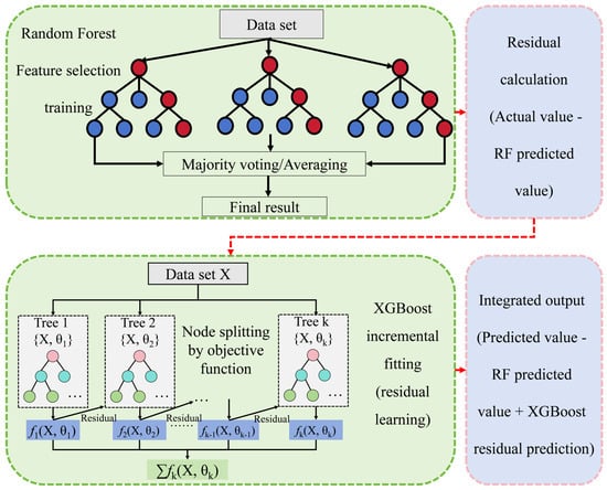
The parallel ensemble architecture of RF allowed for the concurrent training of multiple independent decision trees, with final predictions derived through majority voting or averaging. This structure was particularly effective at identifying dominant and stable patterns in the data; however, the architecture demonstrated reduced sensitivity to minor variations, thereby limiting the model’s capacity to capture subtle, unmolded nuances.

The sequential ensemble methodology of XGBoost enabled each constituent tree to specifically learn the residuals from all preceding trees, thereby progressively reducing bias through iterative refinement. This serial architecture excelled at capturing subtle patterns of deviation; however, when employed in isolation, the approach could predispose the model to overfitting noise due to excessive focus on error minimization.

As illustrated in Figure 5, this study initially employed the RF parallel ensemble framework to capture the overall trend in the data and generate baseline predictions, while simultaneously computing the corresponding residuals, hereinafter referred to as baseline residuals. Subsequently, XGBoost was utilized to learn the mapping between these residuals and the input features, thereby producing residual predictions. The final prediction was derived by summing the baseline and residual predictions. The specific formulation was as follows:

$${\widehat{y}}_t^{RF}=RF(x_{t-L},x_{t-(L+1)},...,x_{t-1})$$

(1)

$$e_t^{RF}=y_t-{\widehat{y}}_t$$

(2)

$${\widehat{e}}_t^{XGB}=XGB(x_{t-L},x_{t-(L+1)},...,x_{t-1},{\widehat{y}}_t^{RF})$$

(3)

$${\widehat{y}}_t^{final}={\widehat{y}}_t^{RF}+{\widehat{e}}_t^{XGB}$$

(4)

where ${\widehat{y}}_t^{RF}$ was the base prediction value of RF at time t, t was the time step. RF(x_t−L, x_t−(L+1), …, x_t−1) was the random forest model, with the input being the feature sequence of the previous L time steps and the output being the base prediction value at time t. x_t was the input feature vector at time t. L was the length of the time series sequence. $e_t^{RF}$ was the prediction residual of RF. y_t was the true soil temperature at time t. ${\widehat{e}}_t^{XGB}$ was the predicted value of the RF residual by XGBoost. $XGB(x_{t-L},x_{t-(L+1)},...,x_{t-1},{\widehat{y}}_t^{RF})$ represented the mapping function of the XGBoost model. ${\widehat{y}}_t^{final}$ represented the final prediction value of the two-stage model.

Figure 5. Schematic diagram of the integrated model.

2.4. Model Training and Validation

To ensure a rigorous and leakage-free evaluation of the models described in Section 2.2, the dataset was divided into training and test subsets in strict chronological order, consistent with the time-series nature of the data. Specifically, the first 80% of the time-ordered samples (6145 timesteps) were used as the training set, while the remaining 20% (1536 timesteps) were reserved as an independent test set. The test set was completely excluded from model training, cross-validation, and hyperparameter tuning.

Cross-validation was performed exclusively on the training dataset. A 5-fold forward-chaining (time-ordered) cross-validation strategy was adopted to account for temporal dependencies and prevent data leakage. In this approach, the training data were sequentially partitioned into five folds using an expanding window scheme. For each fold, the model was trained on past data and validated on the immediately subsequent subset, ensuring temporal consistency.

To further eliminate potential data leakage, all preprocessing steps were conducted strictly within each training fold. Feature engineering and normalization parameters were derived solely from the training portion and then applied to the corresponding validation subset. In addition, sliding-window input sequences (192 time steps, corresponding to 48 h) were constructed independently within each fold, ensuring that no future information from validation or test periods was included in the model inputs.

For multi-step forecasting, a rolling prediction strategy was employed to generate 12 h ahead soil temperature predictions, allowing the model to iteratively update inputs based on previous predictions and simulate real-time forecasting conditions.

This strict separation between training, validation, and testing procedures ensured an unbiased evaluation of model performance and prevented any form of information leakage.

The model’s testing performance was evaluated using the Mean Squared Error (MSE), Root Mean Squared Error (RMSE), Mean Absolute Error (MAE), and Coefficient of Determination (R²), which were calculated as follows:

$$\mathrm{MSE}={\displaystyle \frac{1}{n}}\sum _{i=1}^n(y_i-{\widehat{y}}_i{)}^2$$

(5)

$$\mathrm{RMSE}=\sqrt{{\displaystyle \frac{1}{n}}\sum _{i=1}^n(y_i-{\widehat{y}}_i{)}^2}$$

(6)

$$\mathrm{MAE}={\displaystyle \frac{1}{n}}\sum _{i=1}^n\left|y_i-{\widehat{y}}_i\right|$$

(7)

$$R^2=1-{\displaystyle \frac{{\sum }_{i=1}^n(y_i-{\widehat{y}}_i{)}^2}{{\sum }_{i=1}^n(y_i-{\overline{y}}_i{)}^2}}$$

(8)

where y_i was the true value of the i-th sample. ${\widehat{y}}_i$ was the predicted value of the i-th sample. ${\overline{y}}_i$ was the sample mean of the dependent variable.

3. Results

3.1. Soil Temperature Dynamics in the Solar Greenhouse

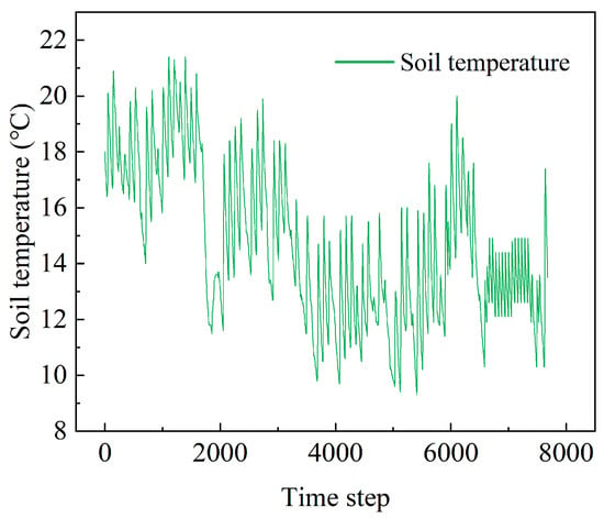
To provide an overall understanding of soil temperature dynamics during the experimental period, Figure 6 presents the measured soil temperature time series from December to February. The data exhibit clear temporal variations influenced by changes in outdoor temperature and solar radiation.

Figure 6. Time series of measured soil temperature during the experimental period.

Overall, soil temperature demonstrates pronounced diurnal patterns and gradual responses to external meteorological conditions, reflecting the thermal inertia and buffering capacity of the greenhouse soil. Notably, significant fluctuations can be observed during extreme weather events, such as cold waves and prolonged low-radiation periods.

To further investigate these dynamics, the following sections analyze soil temperature variations in relation to meteorological conditions on a monthly basis.

3.1.1. Meteorological Conditions and Soil Temperature Threshold

The thermal energy requirement for greenhouse soil depends on both crop characteristics and external meteorological conditions, particularly outdoor air temperature and solar irradiation. To provide a comprehensive description of the environmental conditions during the experimental period, Table 2 summarizes the monthly statistics of outdoor temperature and daily solar irradiation, including maximum, minimum, mean, and standard deviation values.

Table 2. Monthly values of outdoor temperature and solar radiation.

Month	Outdoor Temperature (°C)				Solar Radiation (MJ m−2 d−1)
	Maximum	Minimum	Average	Standard Deviation	Maximum	Minimum	Average	Standard Deviation
December	15.0	−15.4	−1.1	6.1	7.3	0.4	4.5	2.4
January	9.1	−21.6	−6.7	6.8	6.6	0.1	3.6	2.1
February	5.7	−22.0	−9.2	5.8	7.0	0.1	4.2	2.2

The results indicate substantial temporal variability in both temperature and solar energy input during the winter season. Outdoor air temperature exhibited large fluctuations, with minimum values reaching as low as −22.0 °C in February and daily variations reflected by standard deviations of 5.8–6.8 °C. Meanwhile, the mean daily solar irradiation ranged from 3.6 to 4.5 MJ m⁻² d⁻¹, with considerable variability across days, highlighting the unstable solar energy supply under winter conditions.

This investigation adopts 15 °C as the critical minimum soil temperature threshold for cold-tolerant solanaceous crops (e.g., tomato, eggplant, and pepper). When the greenhouse soil temperature falls below this threshold, heating is required to maintain suitable root-zone thermal conditions. This criterion is supported by agronomic studies indicating that root-zone temperatures below 12–15 °C significantly impair nutrient uptake and root activity, with irreversible growth inhibition occurring below 12 °C [9].

3.1.2. Soil Temperature Variation in December

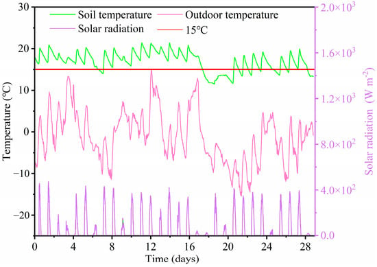
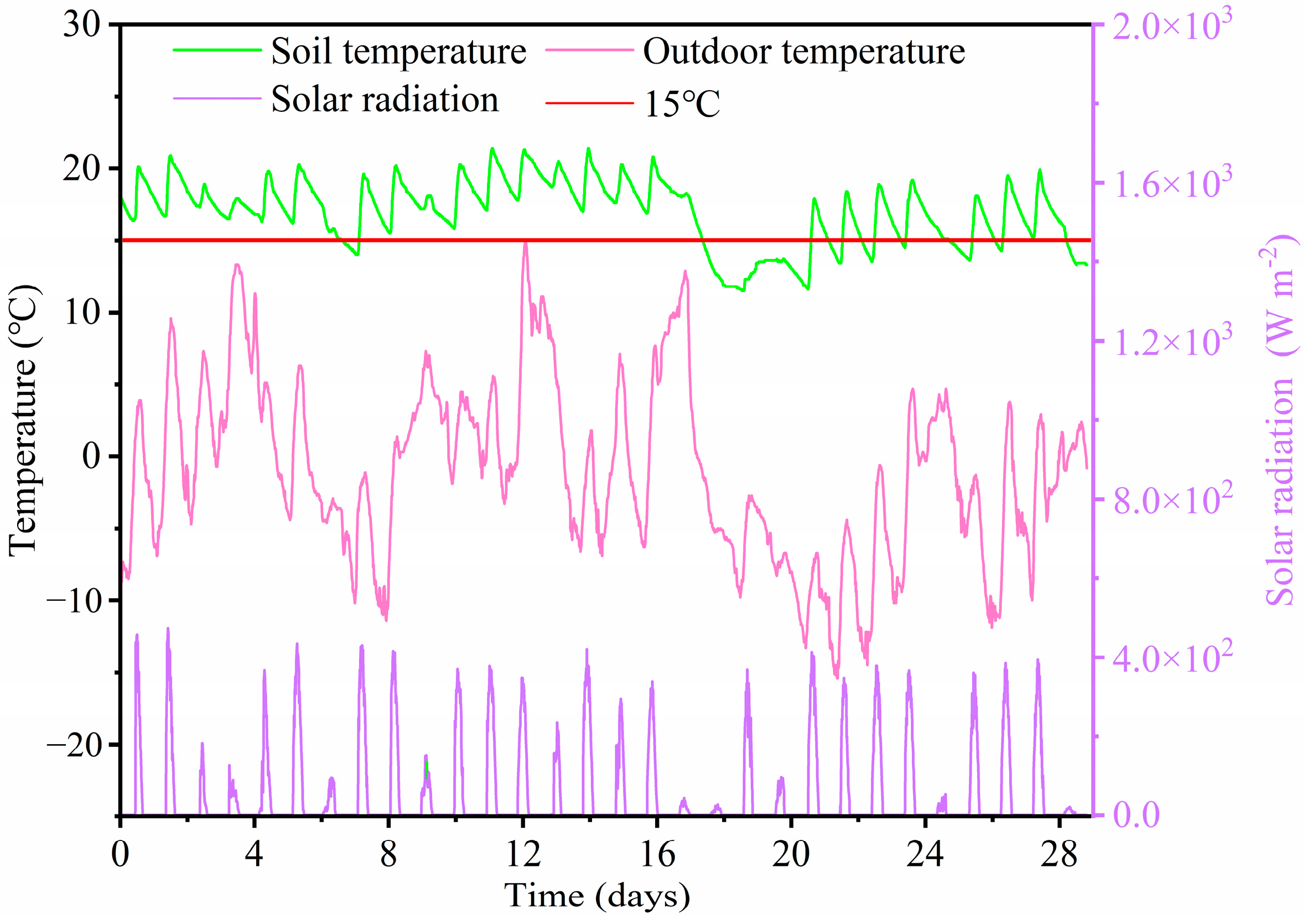
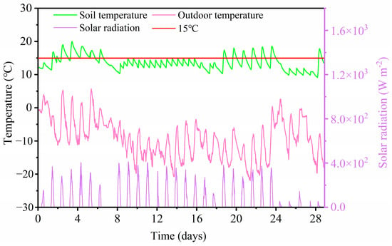
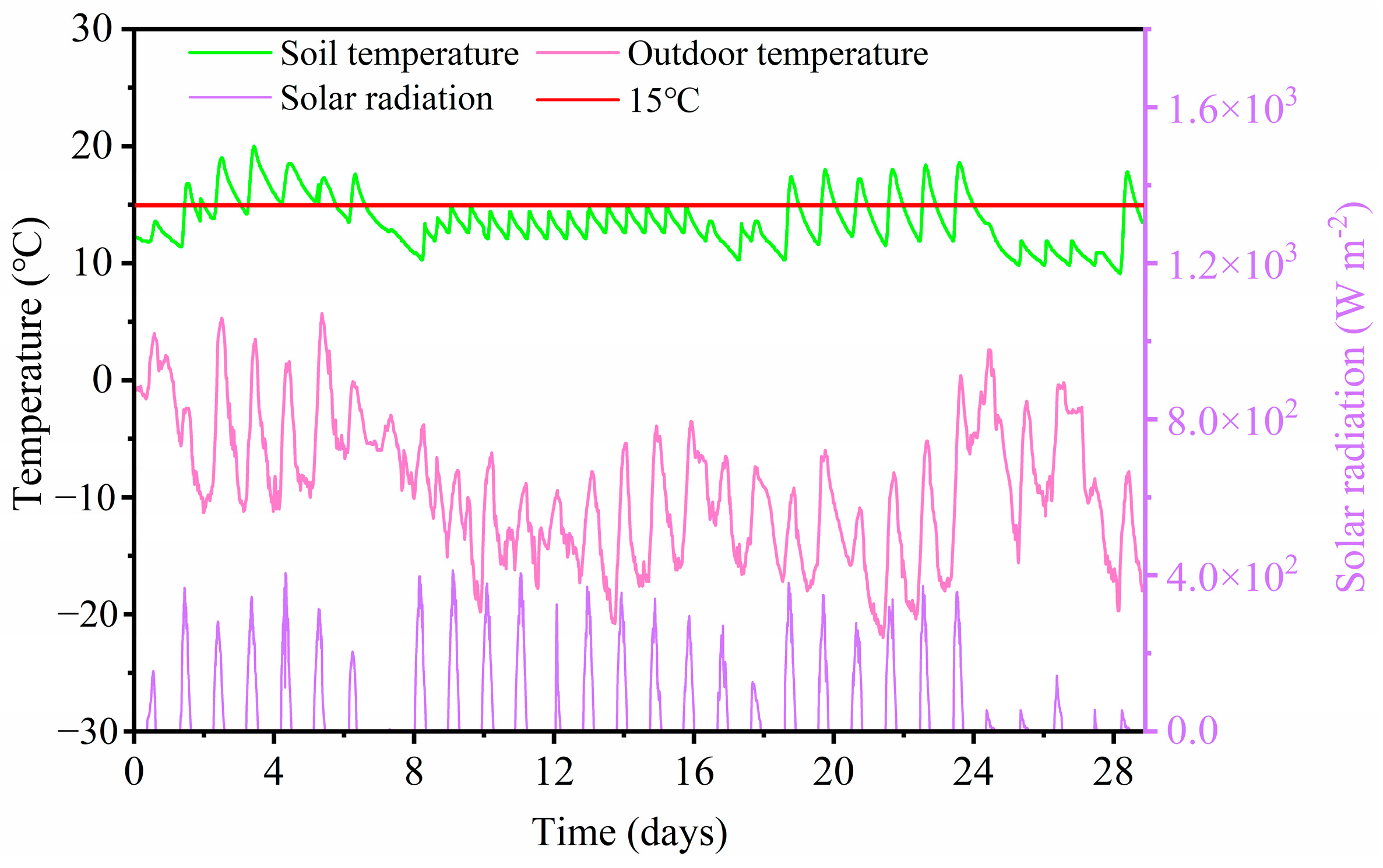
Figure 7 illustrates the variation in soil temperature inside the greenhouse during December in relation to outdoor temperature and solar radiation. It should be noted that no active or auxiliary heating system was operated during the monitoring period; therefore, all observed variations reflect the passive thermal performance of the greenhouse under natural environmental conditions.

Figure 7. Soil temperature variation in the greenhouse during December relative to outdoor temperature and solar radiation.

The greenhouse soil temperature was influenced by both outdoor temperature and solar radiation. For most of December, the average soil temperature remained above 15 °C without external heating, indicating adequate thermal buffering capacity. However, on December 17–18, snowfall events led to a sharp reduction in solar radiation, with maximum daily values below 50 W m⁻². Subsequently, outdoor temperature dropped significantly from December 19 and remained low for three consecutive days. During this period, the greenhouse’s passive thermal regulation was insufficient to maintain optimal conditions for crop growth. The maximum and minimum outdoor temperatures decreased by approximately 20 °C and 15 °C, respectively, with an average of −13 °C. Correspondingly, the soil temperature declined markedly, with reductions of about 8 °C in maximum values and 5 °C in minimum values. The average soil temperature from December 17 to 21 was approximately 13 °C. This indicates that auxiliary heating would be required to raise the soil temperature by approximately 2 °C within five days to maintain suitable root-zone conditions and avoid potential adverse effects on crop growth.

3.1.3. Soil Temperature Variation in January

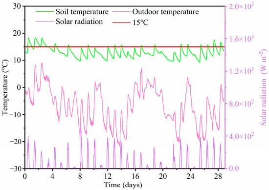
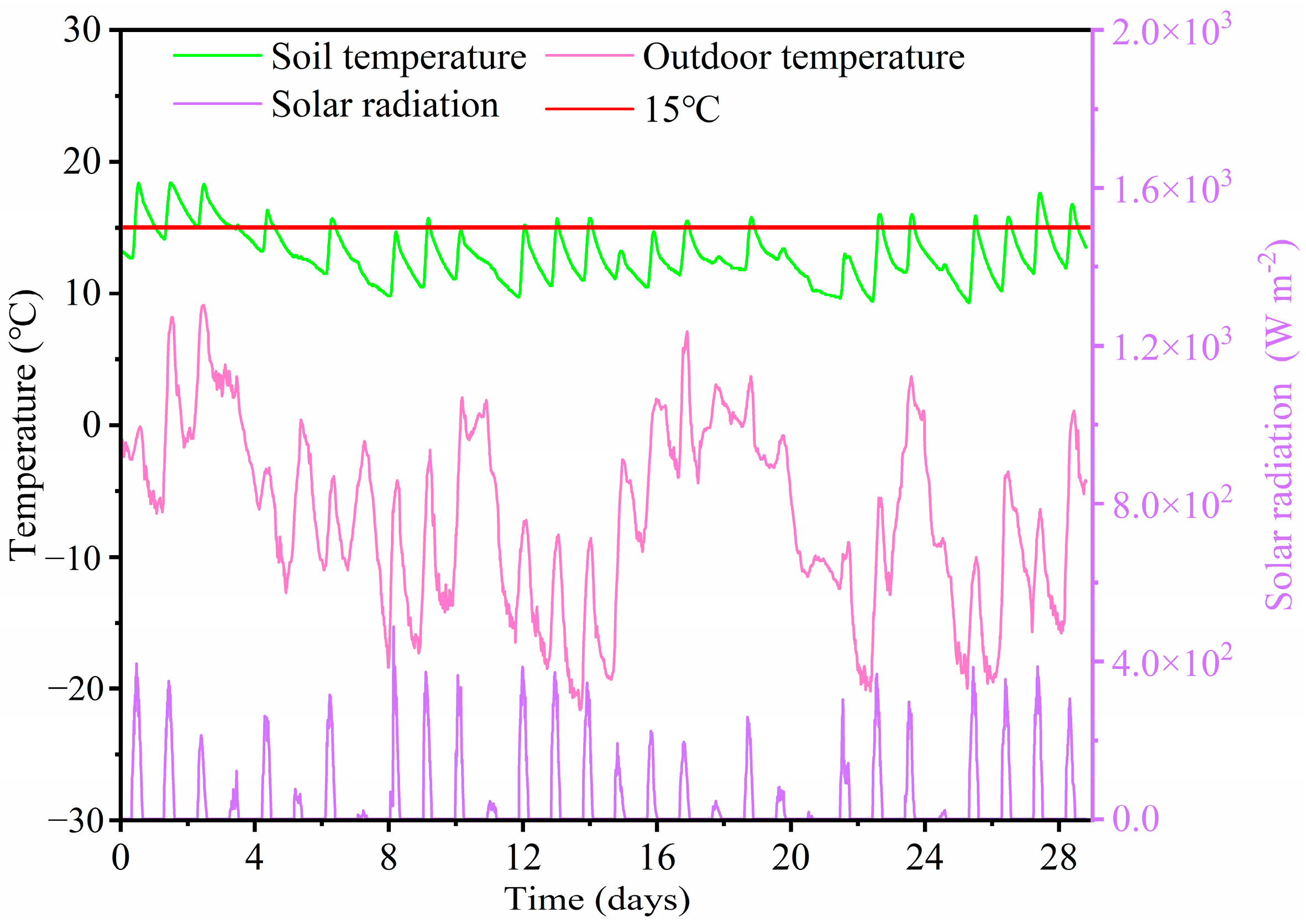
Figure 8 presents the variation in soil temperature inside the greenhouse during January relative to outdoor temperature and solar radiation. As shown in Figure 8, outdoor temperature decreased continuously from January 6 to 14, with the minimum temperature dropping from −8 °C to −22 °C, followed by a gradual increase between January 15 and 25. During this latter period, three consecutive overcast days occurred, with maximum daily solar radiation below 40 W m⁻².

Figure 8. Soil temperature variation in the greenhouse during January relative to outdoor temperature and solar radiation.

Under these combined conditions of low temperature and limited solar input, the greenhouse soil temperature fluctuated around 15 °C, demonstrating a certain degree of thermal inertia and buffering capacity. However, this passive regulation was not sufficient to consistently maintain optimal root-zone temperatures. The minimum soil temperature remained below 15 °C for extended periods, and the average soil temperature from January 6 to 25 was approximately 14 °C.

These results suggest that, under prolonged low-temperature and low-radiation conditions, auxiliary heating would be required to increase soil temperature by approximately 1 °C over a 20-day period to ensure stable crop growth.

3.1.4. Soil Temperature Variation in February

Figure 9 illustrates the variation in soil temperature inside the greenhouse during February in relation to outdoor temperature and solar radiation. A significant cooling period began on February 7, during which outdoor temperature decreased continuously over the following week, reaching a maximum of approximately −10 °C and a minimum of −22 °C. Even under relatively favorable solar radiation conditions, prolonged exposure to low ambient temperatures resulted in persistently low soil temperatures. Between February 7 and 16, the average soil temperature was maintained at approximately 13 °C.

Figure 9. Soil temperature variation in the greenhouse during February relative to outdoor temperature and solar radiation.

Later, from February 24 to 28, the greenhouse experienced continuous snowfall and cold weather, with maximum daily solar radiation below 50 W m⁻² and an average outdoor temperature of −13 °C. Under the combined effects of low temperature and limited solar input, soil temperature decreased sharply and remained at low levels for several days. During this period, the average soil temperature was approximately 11 °C, which is below the threshold required for normal crop growth.

These conditions indicate that sustained auxiliary heating would be required to increase soil temperature by approximately 2–4 °C within several days to restore a suitable thermal environment for plant development.

3.2. Machine Learning Prediction of Soil Temperature in Solar Greenhouses

3.2.1. Factor Correlation Analysis

In machine learning applications, proper evaluation of training and testing datasets is crucial for mitigating issues such as underfitting, overfitting, and multicollinearity. At the outset of the analysis, this study examined whether multicollinearity existed among the input parameters. The Variance Inflation Factor (VIF) values were determined as follows: solar radiation (4.588), outdoor temperature (1.556), indoor temperature (8.820), and soil temperature (3.758). VIF values below 10 are generally considered to indicate the absence of serious multicollinearity; therefore, the variables used in this study do not exhibit significant multicollinearity. The moderate correlation between indoor and outdoor temperature (ρ = 0.52) does not compromise model stability, as both variables represent distinct physical mechanisms: indoor temperature reflects the greenhouse’s thermal buffer capacity, while outdoor temperature represents the external boundary condition.

Variable selection was based on physical consideration of the greenhouse energy balance. Indoor temperature serves as the direct convective heating source for the soil surface, outdoor temperature defines the external thermal gradient driving heat loss through the north wall and foundation, and solar radiation provides the primary energy input captured through the transparent south roof. These three variables collectively represent the dominant forcing mechanisms in the soil–plant–atmosphere system, with soil moisture held constant through controlled irrigation and thus excluded from the predictive model.

To capture nonlinear dependencies and time-lagged relationships critical to soil thermal dynamics, we employed complementary analytical approaches beyond simple linear correlation. Spearman rank correlations were calculated to assess monotonic nonlinear relationships. Cross-correlation analysis revealed that indoor temperature leads soil temperature by 3–4 h (peak correlation at lag 16 timesteps, ρ = 0.89), while solar radiation leads by 1–2 h (peak at lag 6, ρ = 0.41), explicitly quantifying the thermal hysteresis that complicates predictive modeling. Mutual information analysis further revealed nonlinear dependencies: solar radiation and soil temperature share 0.45 bits of mutual information versus a linear correlation of ρ = 0.32, confirming that radiation effects on soil temperature involve nonlinear threshold behaviors (e.g., radiation deficit accumulation over multiple days).

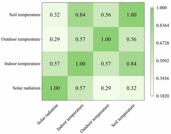
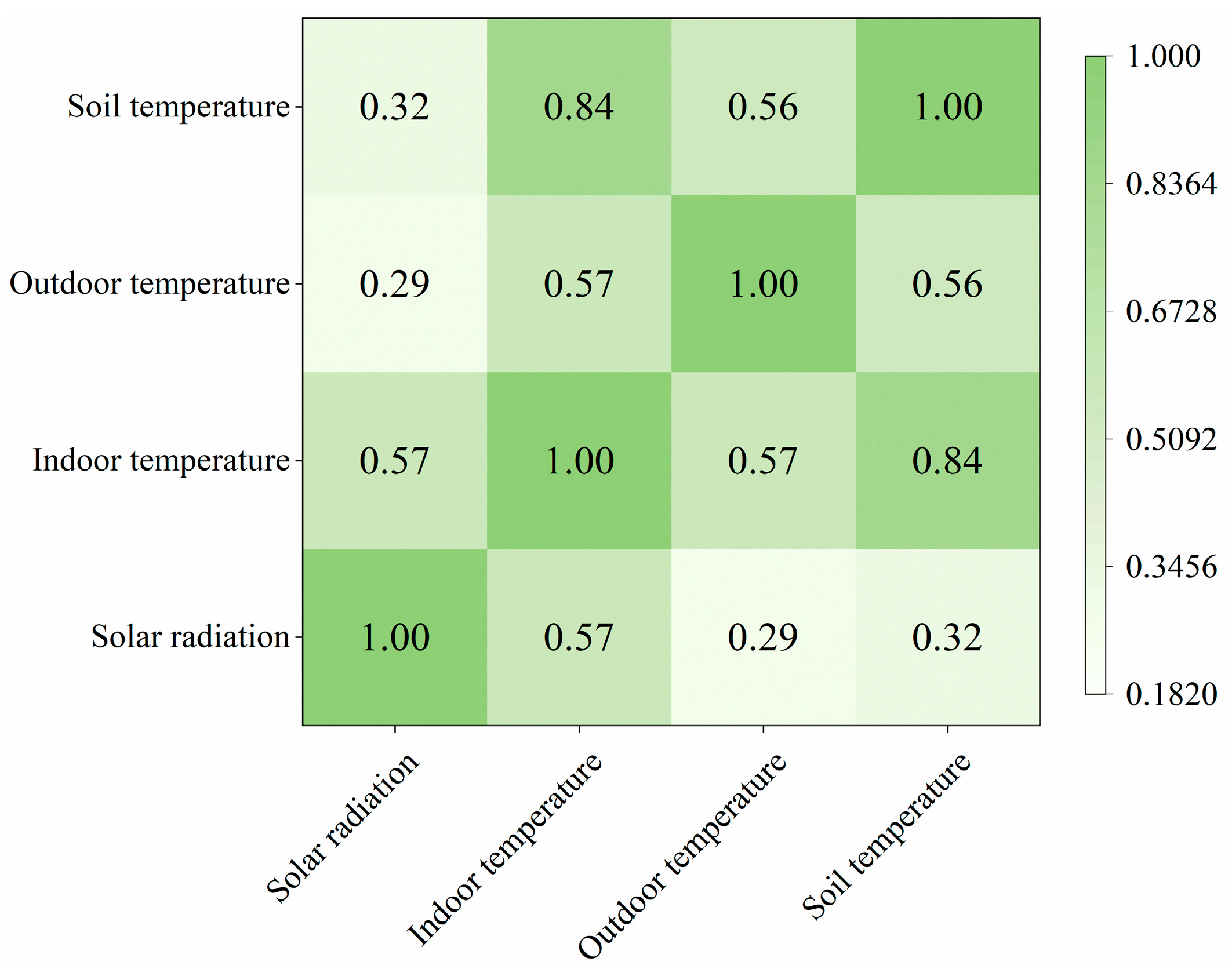
Figure 10 presents the Spearman rank correlation heatmap revealing the monotonic relationships among solar radiation, indoor temperature, outdoor temperature, and soil temperature. Strong positive correlations were observed between indoor temperature and soil temperature (ρ = 0.84, p < 0.001), and between outdoor temperature and soil temperature (ρ = 0.56, p < 0.001), confirming the dominant influence of indoor temperature on soil thermal conditions. In contrast, solar radiation showed weak associations with both soil temperature (ρ = 0.32, p < 0.001) and outdoor temperature (ρ = 0.29, p < 0.001). Notably, all correlations achieved statistical significance (p < 0.001), validating the reliability of these relation-ships regardless of their magnitude.

Figure 10. Correlation heatmap.

3.2.2. Basic Model Analysis

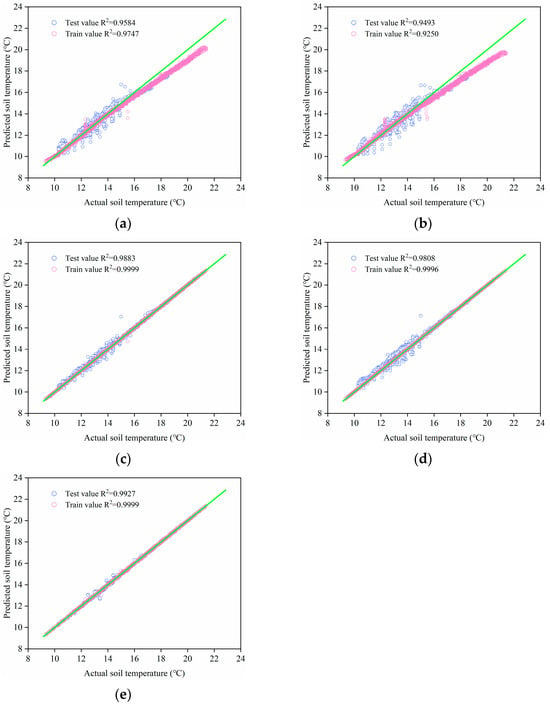
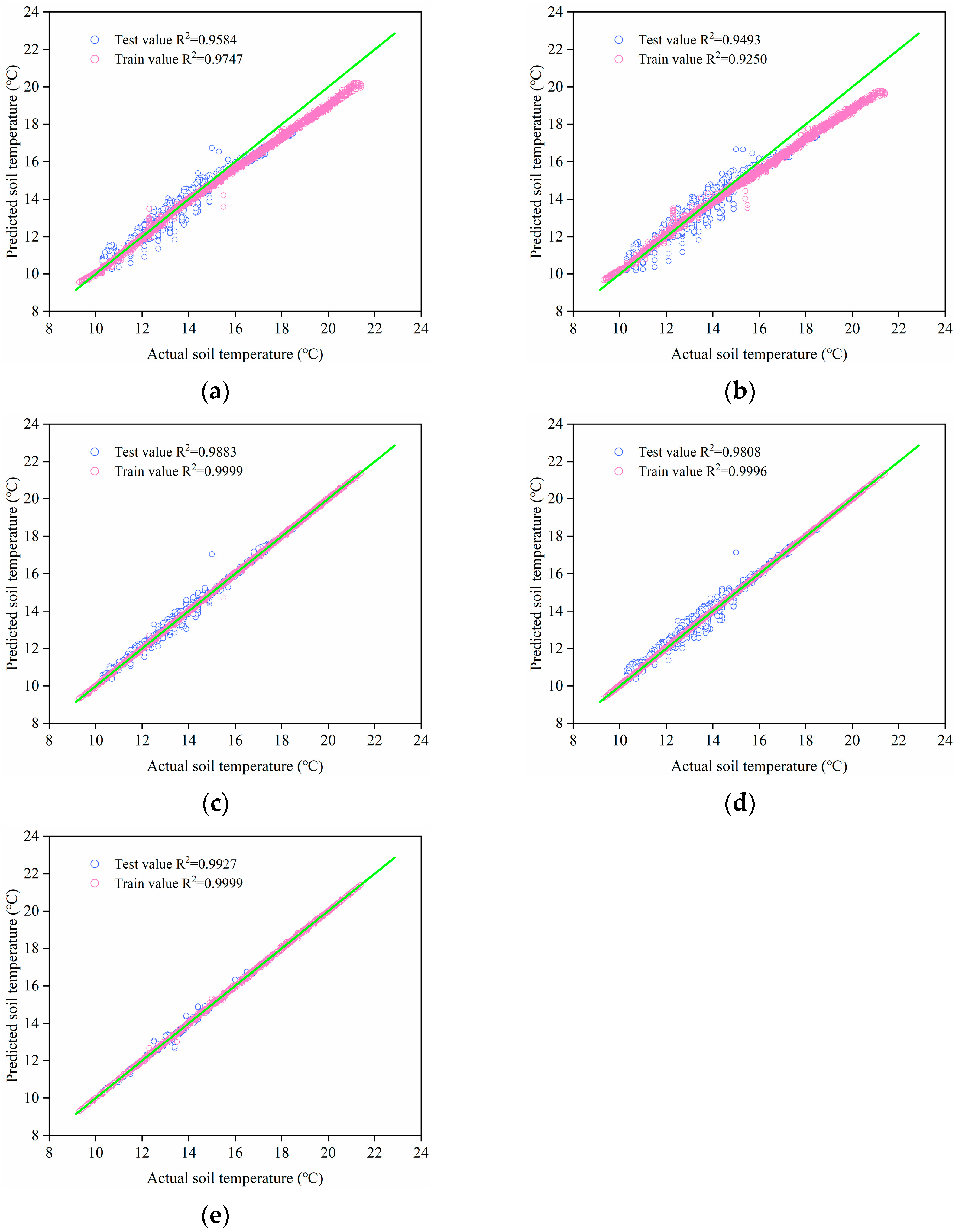
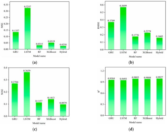
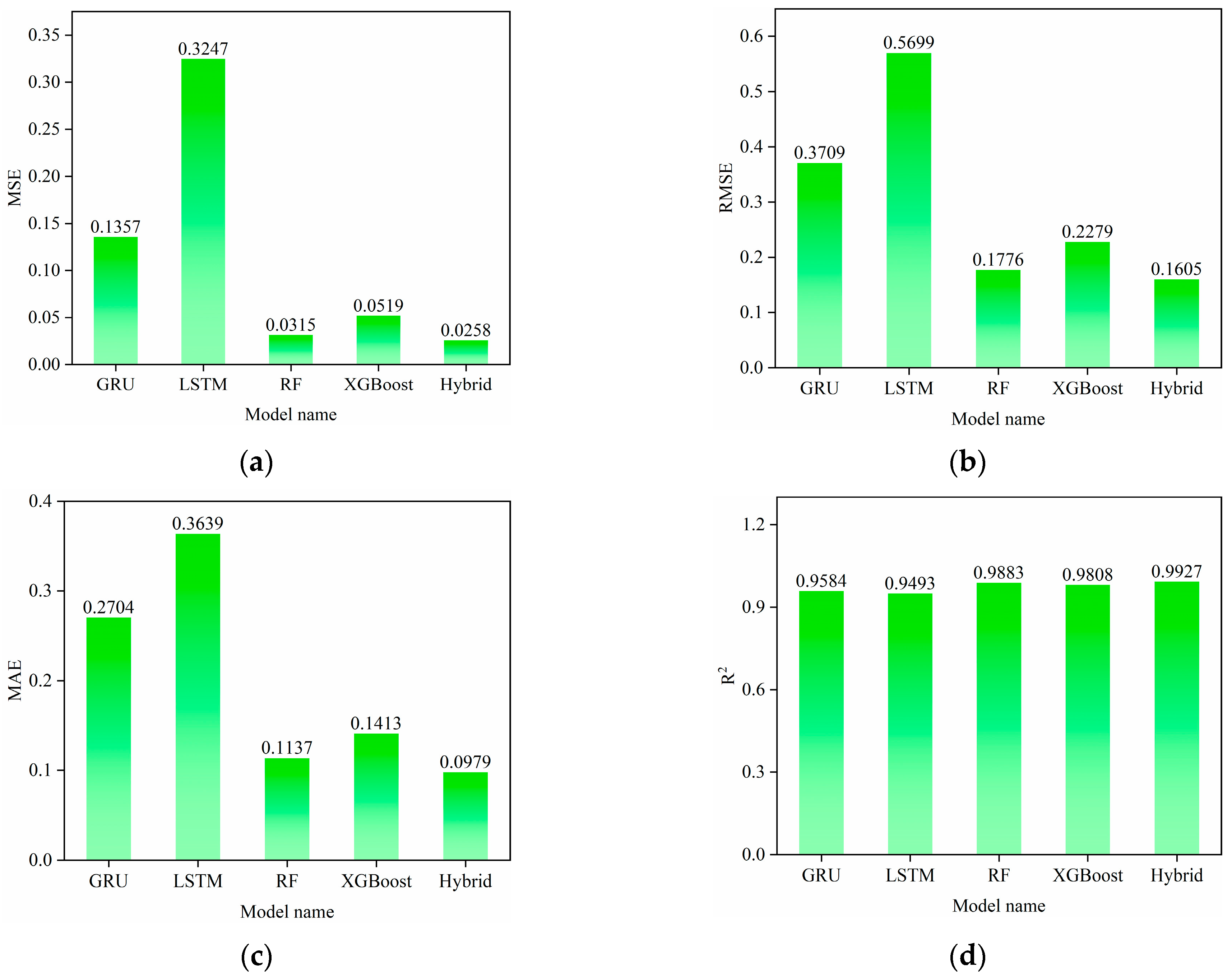
Figure 11 and Figure 12 present the comparative performance of the four baseline models for soil temperature prediction in solar greenhouses, evaluated using four metrics: MSE, RMSE, MAE, and R².

Figure 11. Scatter plots of predicted versus measured soil temperatures for different models: (a) GRU, (b) LSTM, (c) RF, (d) XGBoost, and (e) RF–XGBoost. The green solid line denotes the 1:1 reference line, and model performance is evaluated using the coefficient of determination (R²).

Figure 12. Evaluation indicators: (a) MSE; (b) RMSE; (c) MAE and (d) R².

As illustrated in the figures, the RF model consistently outperforms the other models, achieving the lowest values for MSE, RMSE, and MAE, along with the highest R² value of 0.9883, indicating excellent predictive accuracy and strong model fit. This superior performance is further confirmed by its stability across different cross-validation folds. In addition, permutation testing demonstrates that the model performance is statistically significant and exceeds random chance (p < 0.001). The learning curve analysis shows that the training and validation errors gradually converge as the sample size increases, suggesting that the model generalizes well and that the dataset is sufficient, with no evident signs of overfitting.

RF outperforms sequential models specifically under two critical conditions: (1) rapid temperature transitions, such as cold snap onset, where LSTM’s temporal memory introduces adaptive lag; and (2) stable clear-sky periods with strong diurnal cycles, where RF’s recursive partitioning captures periodic nonlinearities more efficiently than LSTM’s gated smoothing mechanisms. Conversely, LSTM shows advantages during gradual cloudy-period transitions, explaining its intermediate performance. This conditional pattern relates directly to greenhouse physics: RF excels when radiation-driven diurnal patterns dominate, while sequential models better handle convective, slowly varying conditions. The thermal inertia of soil (quantified in Section 3.1) creates distinct regimes—rapid radiation-forced changes versus buffered convective equilibration—that favor different algorithmic architectures.

Error analysis by temperature range reveals all models show higher RMSE in extreme stress conditions versus optimal range, with RF maintaining the smallest degradation. During extreme events such as the December cold snap, RF achieves lower RMSE than XGBoost and LSTM during transition periods, validating its robustness for critical agricultural decisions. Lag analysis indicates RF predictions maintain relatively consistent accuracy across the 0–12 h horizon, while LSTM shows greater degradation as temporal dependencies lengthen, suggesting RF’s superior stability for the target prediction window.

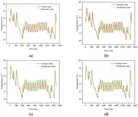
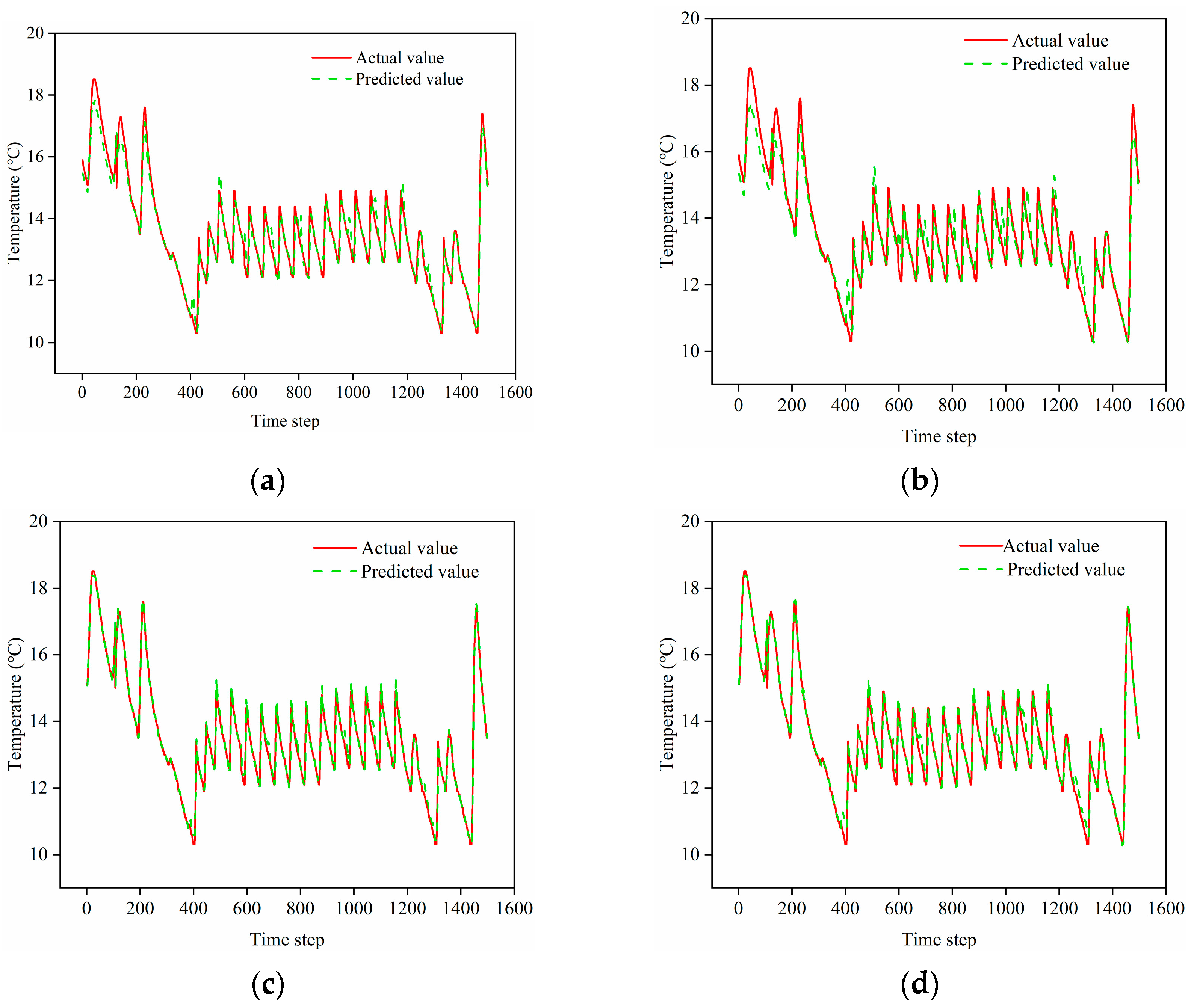
Temporal stability is demonstrated by consistent RF performance across monthly validation sets (December, January, February), with no significant degradation in February’s extreme conditions. Generalizability is supported by maintained performance under documented stress events (cold snap, consecutive overcast days) where single models exhibit pronounced volatility. Figure 13 presents a visual comparison between observed and predicted temperature values over time in the test set, providing an intuitive illustration of comparative prediction accuracy across the models.

Figure 13. Comparison of test set predictions: (a) GRU; (b) LSTM; (c) RF and (d) XGboost.

3.2.3. Error Correction of RF with XGBoost

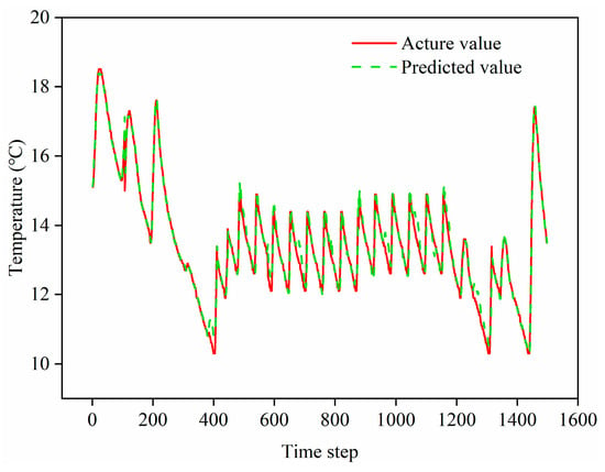
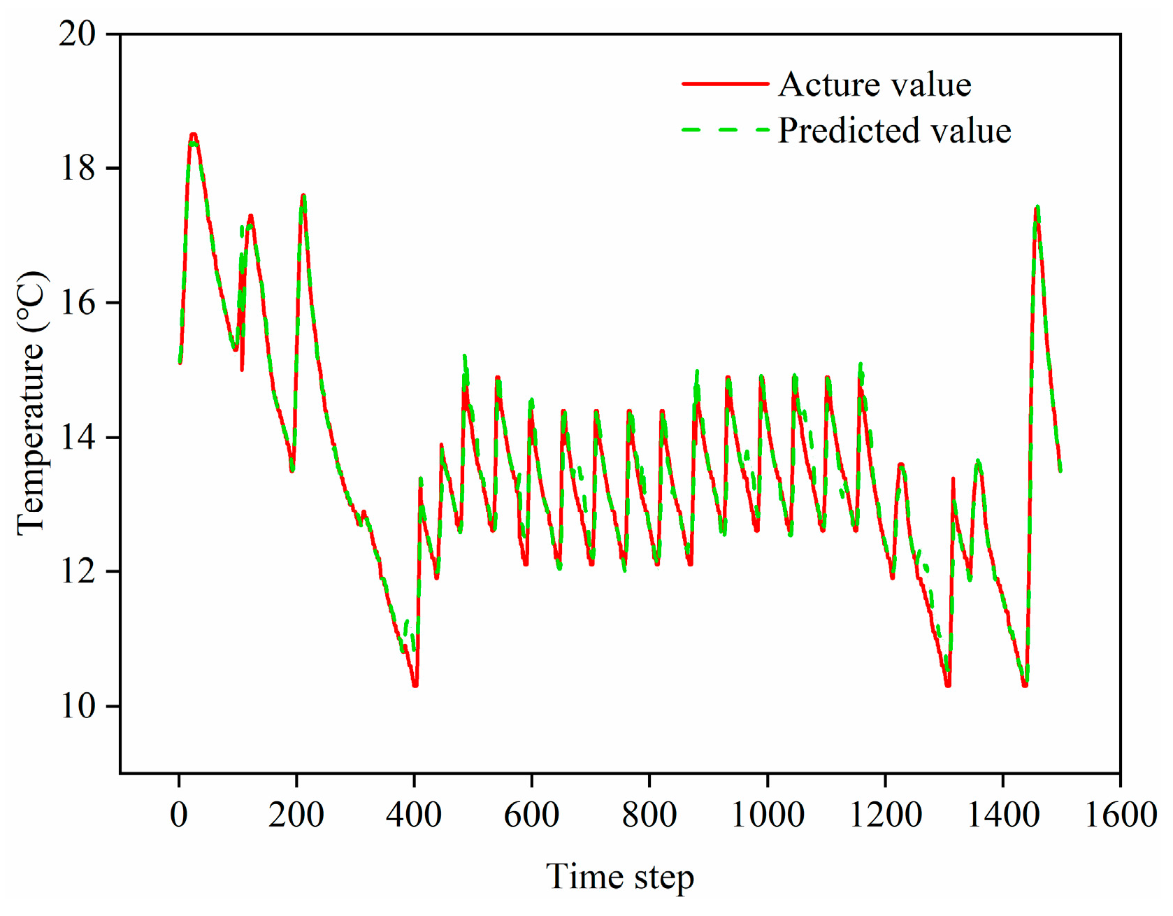
This study proposes an integrated model for predicting soil temperature in solar greenhouses. The model combines an optimized RF base model with an error correction mechanism based on XGBoost through a two-stage training framework, thereby enhancing the prediction accuracy. Comparative analysis of prediction errors indicates that the introduction of XGBoost significantly reduces the inherent systematic bias and variability of the base RF model. Specifically, the MSE decreased from 0.0315 to 0.0258 (an 18.1% reduction), the RMSE from 0.1776 to 0.1605 (a 9.6% reduction), and the MAE from 0.1137 to 0.0979 (a 13.9% reduction), while improving R² by 0.45%. These results demonstrate that the proposed error correction strategy can effectively capture and correct the residuals in the base model’s predictions. Figure 14 presents a visual comparison between the observed and predicted temperatures in the test set, clearly illustrating the improved performance of the ensemble model in forecasting soil temperature within solar greenhouses.

Figure 14. Comparison of observed and predicted soil temperatures using the hybrid RF–XGBoost model.

Following comprehensive evaluation of multiple models through iterative training and validation, model reliability was assessed at the 12 h prediction horizon. Table 3 presents the prediction errors of all evaluated models at this time point. The hybrid RF–XGBoost model achieved the lowest prediction error of 2.52 °C, indicating that this configuration represents the optimal solution.

Table 3. The prediction result of the 12th hour time step.

Prediction Model	True Value (°C)	Predicted Value (°C)	Error (°C)
GRU	16	12.25	3.75
LSTM	16	12.85	3.15
RF	16	12.88	3.12
XGBoost	16	11.40	4.60
Hybrid RF–XGBoost	16	13.48	2.52

It is noteworthy that while the hybrid RF–XGBoost model demonstrates superior overall metrics, a more granular analysis of Figure 14 and Table 3 reveals a non-uniform error distribution across different temperature ranges. Specifically, at extreme low-temperature boundaries, the model occasionally exhibits a slight overestimation, which may pose a potential risk in agricultural practice by delaying the activation of frost-protection systems. Conversely, localized underestimation (underfitting) as observed in specific instances in Table 3 indicates that the complex thermal lag of the soil is not yet perfectly captured under all transient conditions. This discrepancy suggests that while the RF-XGBoost framework effectively reduces systematic bias, its reliability at extreme boundaries could be further enhanced. Future research should consider incorporating physical heat transfer constraints—such as Informed Machine Learning—to calibrate these critical deviations and provide a more robust decision-making basis for greenhouse thermal management.

Beyond statistical accuracy, the high R² and low RMSE achieved by the hybrid RF-XGBoost model have direct implications for precision greenhouse management. A 12 h prediction horizon provides a sufficient ‘lead time’ for greenhouse operators to implement preemptive measures. For instance, the model’s ability to forecast a significant drop in soil temperature allows for the early deployment of thermal blankets or the pre-heating of the greenhouse environment, thereby avoiding the ‘thermal shock’ to crop roots that often occurs when reactive heating is used. This proactive management approach not only optimizes the growth environment for heat-demanding crops like tomatoes and peppers but also contributes to energy efficiency by reducing reliance on emergency high-power heating.

4. Discussion

4.1. Comparison with Existing Models

To further evaluate the effectiveness of the proposed model, a comparison with existing soil temperature prediction approaches is conducted. Previous studies have explored various machine learning models for greenhouse root-zone temperature prediction, providing valuable benchmarks for the present work. Kucukerdem and Ozturk [21] applied XGBoost to predict root-zone temperature in a greenhouse with PCM-based thermal storage, achieving an R² of 0.97, with PCM temperature identified as the most influential predictor. Similarly, Kucukerdem [20] employed XGBoost to predict root-zone temperature under row cover and mulch treatments, achieving RMSE values as low as 0.15–0.19 °C and R² > 0.99, with adjacent soil depths emerging as dominant predictors. Both studies confirmed XGBoost’s strong predictive capability and highlighted the value of feature importance analysis for model interpretability. However, these studies employed single-model XGBoost frameworks, which, as demonstrated by Li et al. [23], may suffer from error accumulation in multi-step forecasting scenarios.

Moreover, recent studies have attempted to incorporate physical insights into data-driven models. Cheng et al. [3] introduced soil temperature zoning and marginal effect analysis to describe spatial variability and boundary effects within greenhouse environments, while also employing simplified solar radiation models to explain soil temperature dynamics. These efforts highlight the importance of integrating physical mechanisms to improve model interpretability.

Despite these advances, most existing models still face notable limitations. Li et al. [23] showed that attention-based LSTM models perform well in short-term forecasting but exhibit performance degradation in multi-step prediction due to error accumulation. Similarly, Wang et al. [27] demonstrated that transformer-based models can enhance feature representation but require large datasets and involve complex architectures, which may limit their real-time applicability in greenhouse control systems.

On the other hand, mechanistic modeling approaches provide strong physical interpretability. Taki et al. [29] highlighted that models based on heat transfer and energy balance can effectively describe greenhouse thermal dynamics; however, these models are often difficult to implement due to complex parameter calibration and sensitivity to environmental variability. This reflects a fundamental trade-off between physical interpretability and predictive flexibility.

Compared with the above approaches, the proposed RF–XGBoost hybrid model achieves an R² of 0.9927 for a 12 h prediction horizon, demonstrating superior performance in long-term forecasting. The two-stage framework separates trend learning and residual correction, effectively reducing error accumulation and improving robustness under dynamic environmental conditions.

Therefore, the proposed model provides a balanced solution by combining high prediction accuracy, computational efficiency, and robustness, making it particularly suitable for practical greenhouse applications that require reliable long-horizon soil temperature forecasting.

4.2. Practical Deployment Considerations

Although the proposed model demonstrates high predictive accuracy under the monitored greenhouse conditions, several factors should be considered for practical deployment.

First, computational efficiency is critical for real-time greenhouse monitoring systems. The RF–XGBoost model has low computational complexity, enabling efficient deployment on edge devices or cloud platforms. In modern smart greenhouse systems, which typically adopt multi-layer architectures integrating sensing, networking, and data processing, lightweight and efficient models are essential for real-time prediction and control [30].

Second, prediction latency must support real-time decision-making. The proposed model generates a 12 h forecast within milliseconds, making it suitable for integration into greenhouse decision-support systems. Predictive models have been widely used to support greenhouse climate management and control, as shown by Ferreira et al. [31].

Third, long-term stability should be considered. Environmental conditions and management practices may change over time, and periodic retraining using updated seasonal datasets is recommended to maintain model performance.

Finally, further validation is required to assess the robustness and generalizability of the proposed model. The current study is based on a single greenhouse and a limited set of input variables (indoor and outdoor temperature, and solar radiation), while other factors were excluded due to their limited variability or strong correlation under the experimental conditions. Future work should incorporate multi-factor datasets and multi-site validation to improve model scalability.

5. Conclusions

This study developed and validated a hybrid machine learning framework for 12 h ahead soil temperature prediction in solar greenhouses, addressing the critical need for proactive thermal management under cold climatic conditions. We systematically compared the predictive performance of standalone models (LSTM, GRU, RF, XGBoost) and a novel two-stage ensemble approach.

Results demonstrate that tree-based models (RF and XGBoost) significantly outperformed recurrent neural networks (LSTM and GRU) for this task, with RF achieving the highest accuracy among standalone configurations. This superiority reflects the effectiveness of ensemble tree methods in capturing the complex nonlinear relationships between environmental drivers (indoor/outdoor temperature, solar radiation) and soil thermal dynamics, despite the inherent temporal dependencies in the data.

The proposed RF-XGBoost hybrid model, which employs RF for baseline prediction and XGBoost for residual error correction, further improved predictive performance. Compared to the optimal standalone model, the ensemble reduced MSE, RMSE, and MAE by 18.1%, 9.6%, and 13.9%, respectively, while maintaining robust performance at the 12 h prediction horizon with a maximum error of 2.52 °C. These findings validate that integrating complementary learning strategies—Bagging for dominant trend capture and Boosting for bias correction—effectively addresses the thermal hysteresis and non-stationary fluctuations characteristic of greenhouse soil temperature dynamics.

To bridge the gap between theoretical modeling and practical application, this study outlines a framework for integrating the developed algorithms into a smart greenhouse ecosystem. The RF-XGBoost model can be deployed as a cloud-based inference engine within an IoT-enabled monitoring platform. By utilizing real-time data from a limited number of cost-effective air temperature and radiation sensors, the system can provide spatial-temporal soil temperature maps without the need for high-density, expensive underground sensor networks. This approach significantly reduces the initial investment for small-to-medium scale farmers while providing a reliable ‘early warning system’ for root-zone cold stress. Ultimately, the implementation of these data-driven strategies facilitates the transition from experience-based farming to data-informed precision horticulture.

Despite the strong predictive performance of data-driven models, their lack of physical interpretability remains a key limitation. Incorporating physical insights, such as soil temperature zoning, marginal effects, and solar radiation mechanisms, can improve the understanding of soil thermal dynamics. However, these approaches are typically not fully integrated into predictive models.

Future research should therefore focus on integrating physical constraints into data-driven frameworks. This can be achieved by incorporating physically meaningful variables (e.g., cumulative solar radiation, temperature gradients, and soil thermal zones) or by embedding physical laws such as heat conduction and energy balance into model structures or loss functions. Such hybrid approaches are expected to improve model robustness and generalization under extreme or unseen environmental conditions.

References

- Wang, C.; Jiang, Y.; Bai, Y.; Wang, T. Numerical study on static properties and failure mechanisms of landing assembled Chinese solar greenhouses. Comput. Electron. Agric. 2021, 188, 106347. [Google Scholar] [CrossRef] [Scilit]
- Wang, C.; Ma, C.; Tong, G. Effect of crop and side wall shadows on the direct solar radiation gain inside Chinese solar greenhouses. Therm. Sci. Eng. Prog. 2025, 68, 104289. [Google Scholar] [CrossRef] [Scilit]
- Cheng, W.; Wang, C.; Wang, Y.; Hao, L.; Liu, Z.; Cui, Q. Soil marginal effect and LSTM model in Chinese solar greenhouse. Sensors 2024, 24, 4730. [Google Scholar] [CrossRef] [Scilit]
- Wang, C.; Ma, C.; Tong, G. Modeling direct solar radiation shadows in Chinese solar greenhouses. Trans. Chin. Soc. Agric. Eng. 2026, 42, 361–368. [Google Scholar] [CrossRef]
- Hayashi, S.; Levine, C.P.; Yu, W.; Usui, M.; Yukawa, A.; Ohmori, Y.; Kusano, M.; Kobayashi, M.; Nishizawa, T.; Kurimoto, I.; et al. Raising root zone temperature improves plant productivity and metabolites in hydroponic lettuce production. Front. Plant Sci. 2024, 15, 1352331. [Google Scholar] [CrossRef] [Scilit]
- Bantis, F.; Tostsidis, N.; Zervoudakis, G.; Koukounaras, A.; Koulopoulos, A. Root-zone heating boosts the production of mini romaine lettuce grown in nutrient film technique and aeroponics systems. Plants 2026, 15, 422. [Google Scholar] [CrossRef] [Scilit] [PubMed]
- Myung, J.; Cui, M.; Lee, B.; Lee, H.; Shin, J.; Chun, C. Development of a root-zone temperature control system using air-source heat pump and its impact on the growth and yield of paprika. AoB PLANTS 2024, 16, plae047. [Google Scholar] [CrossRef] [Scilit]
- Luo, Q.; Guo, Y.; Dai, A.; Li, Y.; Cheng, J.; Wang, P.; Zhao, S. Research on the evaluation model of soil heat loss in solar greenhouses. Energy 2025, 322, 135665. [Google Scholar] [CrossRef] [Scilit]
- Kawasaki, Y.; Yoneda, Y. Local temperature control in greenhouse vegetable production. Hortic. J. 2019, 88, 305–314. [Google Scholar] [CrossRef] [Scilit]
- Yu, J.; Sun, C.; Zhao, J.; Ma, L.; Zheng, W.; Xie, Q.; Wei, X. Prediction and control of greenhouse temperature: Methods, applications, and future directions. Comput. Electron. Agric. 2025, 237, 110603. [Google Scholar] [CrossRef] [Scilit]
- Chen, P.; Ruan, F.; Li, S.; Qin, D.; Xu, S. Exploring crop root-soil heat relationships to optimally predict soil temperatures in greenhouse spaces. Plant Soil 2024, 505, 595–613. [Google Scholar] [CrossRef] [Scilit]
- Jiao, Y.; Chen, C.; Li, J.; Li, G.; Lan, H.; Han, F.; Zhao, T. Study on soil temperature distribution and cold/heat zoning method of solar greenhouse based on thermal superposition principle. Energy 2025, 314, 134222. [Google Scholar] [CrossRef] [Scilit]
- Bournet, P.-E.; Rojano, F. Advances of Computational Fluid Dynamics (CFD) applications in agricultural building modelling: Research, applications and challenges. Comput. Electron. Agric. 2022, 201, 107277. [Google Scholar] [CrossRef] [Scilit]
- Li, Y.; Jian, Y.; Wang, S.; Liu, X.; Li, W.; Arıcı, M.; Zhang, L.; Li, W.; Cao, Y. Spatial temperature distribution and ground thermal storage in the plastic greenhouse: An experimental and modeling study. J. Energy Storage 2024, 77, 109938. [Google Scholar] [CrossRef] [Scilit]
- Deng, L.; Huang, L.; Zhang, Y.; Li, A.; Gao, R.; Zhang, L.; Lei, W. Analytic model for calculation of soil temperature and heat balance of bare soil surface in solar greenhouse. Sol. Energy 2023, 249, 312–326. [Google Scholar] [CrossRef] [Scilit]
- Jiao, Y.; Chen, C.; Li, G.; Fu, H.; Mi, X. Research on the variation patterns and predictive models of soil temperature in a solar greenhouse. Sol. Energy 2024, 270, 112267. [Google Scholar] [CrossRef] [Scilit]
- Cai, W.; Wei, R.; Xu, L.; Ding, X. A method for modelling greenhouse temperature using gradient boost decision tree. Inf. Process. Agric. 2022, 9, 343–354. [Google Scholar] [CrossRef] [Scilit]
- Yin, H.; Wu, Z.; Huang, Z.; Luo, Y.; Liu, X.; Peng, X.; Li, Q. A multivariate soil temperature interval forecasting method for precision regulation of plant growth environment. Front. Plant Sci. 2024, 15, 1460654. [Google Scholar] [CrossRef] [Scilit] [PubMed]
- Myeni, L.; Nkhase, T.; Rapolaki, R.; Bello, Z.; Moeletsi, M.E. Estimation of soil temperature for agricultural applications in South Africa using machine-learning methods. S. Afr. J. Sci. 2025, 121, 1–11. [Google Scholar] [CrossRef] [Scilit] [PubMed]
- Kucukerdem, H.-K. Prediction of root zone temperature dynamics at effective depth on lettuce production in greenhouse using sensitivity and feature importance analysis with XGBoost. Phyton Int. J. Exp. Bot. 2026, 95, 16. [Google Scholar] [CrossRef] [Scilit]
- Kucukerdem, H.K.; Ozturk, H.H. Machine learning-based prediction of root-zone temperature using bio-based phase-change material in greenhouse. Sustainability 2025, 17, 9455. [Google Scholar] [CrossRef] [Scilit]
- Liu, W.; Han, T.; Wang, C.; Zhang, F.; Xu, Z. Predicting indoor temperature of solar green house by machine learning algorithms: A comparative analysis and a practical approach. Smart Agric. Technol. 2025, 12, 101096. [Google Scholar] [CrossRef] [Scilit]
- Li, X.; Zhang, L.; Wang, X.; Liang, B. Forecasting greenhouse air and soil temperatures: A multi-step time series approach employing attention-based LSTM network. Comput. Electron. Agric. 2024, 217, 108602. [Google Scholar] [CrossRef] [Scilit]
- Cui, X.; Cheng, Y.; Zhang, Z.; Mu, J.; Zhang, W. Integrating multi-strategy improvements to sand cat group optimization and gradient-boosting trees for accurate prediction of microclimate in solar greenhouses. Agriculture 2025, 15, 1849. [Google Scholar] [CrossRef] [Scilit]
- Kablanbek, O.; Adamova, A. Evaluating Machine Learning Models for Greenhouse Temperature Prediction. In Proceedings of the 2025 IEEE 5th International Conference on Smart Information Systems and Technologies (SIST), Astana, Kazakhstan, 14–16 May 2025; pp. 1–6. [Google Scholar]
- Jiang, Y.; Zou, J.; Sui, X.; Zheng, Z.; Pang, X. RIME-CNN-BiLSTM for data-driven precision agriculture: A hybrid model for adaptive temperature and humidity forecasting in solar greenhouses. Comput. Electron. Agric. 2025, 238, 110838. [Google Scholar] [CrossRef] [Scilit]
- Wang, F.; Wang, Y.; Chen, W.; Zhao, C. An improved iTransformer with RevIN and SSA for greenhouse soil temperature prediction. Agronomy 2025, 15, 223. [Google Scholar] [CrossRef] [Scilit]
- Machado, R.M.A.; do Rosário, M.; Oliveira, G.; Portas, C.A.M. Tomato root distribution, yield and fruit quality under subsurface drip irrigation. Plant Soil 2003, 255, 333–341. [Google Scholar] [CrossRef] [Scilit]
- Taki, M.; Abdanan Mehdizadeh, S.; Rohani, A.; Rahnama, M.; Rahmati-Joneidabad, M. Applied machine learning in greenhouse simulation; new application and analysis. Inf. Process. Agric. 2018, 5, 253–268. [Google Scholar] [CrossRef] [Scilit]
- Jeon, Y.-J.; Kim, J.Y.; Hwang, K.-S.; Cho, W.-J.; Kim, H.-J.; Jung, D.-H. Machine learning-powered forecasting of climate conditions in smart greenhouse containing netted melons. Agronomy 2024, 14, 1070. [Google Scholar] [CrossRef] [Scilit]
- Ferreira, P.M.; Faria, E.A.; Ruano, A.E. Neural network models in greenhouse air temperature prediction. Neurocomputing 2002, 43, 51–75. [Google Scholar] [CrossRef] [Scilit]
Disclaimer/Publisher’s Note: The statements, opinions and data contained in all publications are solely those of the individual author(s) and contributor(s) and not of MDPI and/or the editor(s). MDPI and/or the editor(s) disclaim responsibility for any injury to people or property resulting from any ideas, methods, instructions or products referred to in the content. |
© 2026 by the authors. Licensee MDPI, Basel, Switzerland. This article is an open access article distributed under the terms and conditions of the Creative Commons Attribution (CC BY) license.