


Abstract
Accurate crop classification provides fundamental data for agricultural resource management and ecological research. Hyperspectral image (HSI) classification is the core technique for achieving precise crop mapping. However, existing models often suffer from excessive parameters, limited robustness under few-shot conditions, and a trade-off between efficiency and robustness. To address these issues, this paper proposes a Multi-Scale Wavelet Kolmogorov–Arnold Network (MSWKN). The model employs a Two-Branch Feature Extractor (TBFE) to capture both spectral correlations and spatial textures. a Channel Cross-Spatial (CCS) module to suppress background clutter and highlight discriminative regions. A group convolution-based Fixed Wavelet Multi-Scale Convolutional Layer (FW-MSCL) that leverages the time–frequency localization of wavelets and learnable linear combinations to enhance robustness against spectral distortion while reducing parameters. And a Fourier-based Transformer encoder to enable global frequency–space modeling. Experiments on the WHU-Hi-HanChuan and WHU-Hi-HongHu hyperspectral crop datasets show that MSWKN achieves high overall accuracy and performs favorably on few-shot categories. Under lower parameter counts and fast inference conditions, the model demonstrates a reasonable trade-off between accuracy and computational efficiency. Ablation studies and wavelet kernel comparisons further confirm the contribution of each module and the advantage of the wavelet. The proposed framework provides an efficient and robust solution for fine-grained hyperspectral crop classification.
1. Introduction
Farmland, as a key component of terrestrial ecosystems, plays a significant role in regional ecological processes due to its cropping structure [1,2]. Accurate acquisition of crop spatial distribution information is essential for agricultural resource management and ecological research. Conventional assessment methods based on statistical data or medium- to low-resolution remote sensing imagery fail to capture fine-scale heterogeneity at the parcel level [3]. Therefore, there is an urgent need for high-resolution, fine-grained crop classification to support parcel-level and seasonal agricultural resource management and ecological research [4].
Affected by growth stages, physiological structures, chlorophyll content, and biotic and abiotic stresses, different crops exhibit distinctive spectral reflectance characteristics [5,6]. Compared with conventional multispectral remote sensing imagery [7], hyperspectral remote sensing imagery, characterized by rich spectral information, short revisit cycles, and high spatial resolution, can objectively reflect the spatial distribution patterns and spectral responses of surface crops, and it has therefore been widely applied in fine-grained crop classification [8,9]. Numerous studies have demonstrated that hyperspectral imagery can accurately record the reflectance and radiance intensity of ground objects across a large number of narrow and contiguous spectral bands, providing a solid data foundation for precise crop identification and classification [10,11,12].
However, targets in hyperspectral images usually possess complex spatial and spectral characteristics simultaneously, making it difficult for single-scale feature extraction methods to comprehensively capture such intricate information [13]. Although multi-scale spectral–spatial feature extraction approaches improve representation capability, their performance remains limited in complex scenes and under scarce training sample conditions [5,6]. In addition to spectral–spatial features, the limitations of frequency domain feature extraction have also attracted increasing attention [14]. Frequency domain features can effectively complement spatial and spectral representations, enhancing the discriminative capability of classification models [15]. As a fundamental tool for frequency domain analysis, the Fourier transform converts images from the spatial domain to the frequency domain, revealing periodic, directional, and textural information, offering a novel perspective for hyperspectral image classification [16,17]. Applying the fractional Fourier transform (FT) to hyperspectral spectral pixels enables the joint capture of time domain and frequency domain characteristics [18], while selecting the order of the Fourier wavelet transform by maximizing separability can significantly improve classification performance [19].
Although multi-scale and frequency domain features provide richer representational dimensions for hyperspectral image classification, traditional machine learning methods [20,21,22] still struggle to effectively handle such high-dimensional and highly nonlinear features. Early studies primarily relied on feature engineering, which exploited manually designed spectral indices and texture feature and made them combined with conventional classifiers. Ref. [23] explored a hybrid strategy integrating endmember extraction algorithms with spectral unmixing techniques, while Zhang et al. [24] improved classification accuracy by optimizing the selection of discriminative spectral bands. To cope with large memory space and high computational cost of large-scale Unmanned Aerial Vehicle hyperspectral datasets, Wang, Zhao, and Yin [25] proposed an enhanced crop classification approach that integrates feature transformation with random forests. However, these traditional machine learning and feature engineering-based methods are limited, including heavy reliance on expert knowledge, poor adaptability to complex scenes, low computational efficiency, and difficulty in meeting the needs of large-scale crop monitoring. To address these problems, Deep Learning (DL) has gradually become the mainstream method [26]. DL network can effectively extract hyperspectral features without overly depending on human intervention. For example, convolutional neural networks (CNNs), recurrent neural networks (RNNs), and graph neural networks (GNNs), have been widely applied to achieve accurate crop classification [27,28]. Meanwhile, these networks have been improved constantly [29,30]. Nevertheless, these DL models have limitations in capturing global contextual information.
To further enhance global context modeling, Transformer-based frameworks have recently been introduced to meet the requirements of crop classification. For example, in crop semantic segmentation tasks, a hybrid Transformer–U-Net framework was proposed to integrate the global information capture capacity of Transformers with the local detail recovery ability of U-Net, improving both the segmentation of crop region and the accuracy of crop classification [31]. By incorporating crop semantic priors to constrain attention weight distributions, Pi et al. [32] developed a semantic-guided Transformer network to mitigate the intervention of background noise (e.g., weeds and soil shadows) and to alleviate the impact of multi-scale crop patterns (e.g., small patches at the seedling stage and continuous blocks at the mature stage) on crop classification. In addition, Zhang, Li, and Zhen [33] designed a hybrid model based on the Kolmogorov–Arnold Network (KAN), offering a solution for hyperspectral crop classification. Although these models can enhance the accuracy of crop classification, the large number of parameters leads to a decrease in their efficiency, which poses a challenge for the practical application of precision agriculture.
To optimize model performance, researchers have attempted to integrate various optimization algorithms with the Transformer framework. For instance, incorporating the Grasshopper Optimization Algorithm with entropy-based feature fusion into Transformer framework enables intelligent optimization of feature selection and fusion weights, effectively reducing redundant computation while preserving critical spectral–spatial information [34]. Dash et al. [35] effectively addressed the issue of high-dimensional and noisy feature data by embedding dimensionality reduction techniques and Long Short-Term Memory (LSTM) networks into the Transformer framework. Their approach first compresses data dimensionality and suppresses noise, then leverages LSTM to capture spectral–temporal dependencies, and finally utilizes Transformers to model global spatial context, forming a synergistic pipeline of dimensionality reduction, temporal modeling, and global spatial learning. Nevertheless, such methods still struggle to strike a satisfactory balance between classification accuracy and efficiency. More importantly, under limited training sample conditions, the performance of these models tends to degrade significantly [36,37].
To address the challenges of excessive model parameters and the difficulty of balancing computational efficiency and robustness, this study proposes a Multi-Scale Wavelet Kolmogorov–Arnold Network (MSWKN) for precise crop classification. The main contributions of this work are summarized as follows: (1) A Multi-Scale Wavelet Kolmogorov–Arnold Network (MSWKN) is proposed, in which multi-scale wavelet analysis is introduced as the core nonlinear transformation function within the Kolmogorov–Arnold framework. By exploiting the time–frequency localization property of wavelets, the proposed model improves robustness against spectral distortion and enhances the representation capability of hyperspectral features. (2) A group convolution-based Fixed-Wavelet Multi-Scale Convolutional Layer (FW-MSCL) is designed. This layer employs fixed wavelet kernels to perform multi-scale feature extraction, significantly reducing the number of parameters while maintaining model robustness, thereby improving computational efficiency. (3) A Channel Cross-Spatial (CCS) module is integrated with a Fourier transform mechanism to enhance the model’s feature extraction capability and global context modeling through joint spectral–spatial interaction and global frequency domain representation.
The remainder of this paper is organized as follows. Section 2 introduces the materials and methods. Section 3 presents the experimental results and conducts analysis. Section 4 discusses the model performance under different conditions. Section 5 summarizes the findings of this study and elaborates on the implications derived from these conclusions.
2. Materials and Methods
2.1. Materials
2.1.1. Datasets
This study employs the WHU-Hi-HanChuan (HC) and WHU-Hi-HongHu (HH) datasets from the WHU-Hi series developed by Wuhan University [38,39]. Both datasets were collected using unmanned aerial vehicles (UAVs) equipped with hyperspectral imaging sensors (Wuhan, China) and are primarily utilized for agricultural remote sensing and crop classification research.
The HC dataset was acquired during the summer in an urban–rural transition area of Hanchuan City, Hubei Province. Captured by a UAV-mounted hyperspectral sensor, it provides a spatial resolution of 0.109 m and includes seven crop species such as strawberry and cowpea. The sample distribution is summarized in Table 1. Characterized by moderate spatial resolution, this dataset is notably influenced by shadow effects, which complicates crop discrimination. Moreover, it contains a limited number of crop classes and lacks closely related varieties.
Table 1.
Class Distribution of the WHU-Hi-HanChuan (HC) Dataset.
In contrast, the HH dataset was collected in winter across a purely agricultural region of Honghu City. It exhibits a higher spatial resolution of 0.043 m and encompasses a broader diversity of crops along with closely related varieties, as detailed in Table 2. Although richer in spatial detail, this dataset is subject to varying illumination conditions, yet it effectively captures the inherent complexity and heterogeneity typical of farmland landscapes.
Table 2.
Class Distribution of the WHU-Hi-HongHu (HH) Dataset.
2.1.2. Data Preprocessing
Before commencing the experiment, we first performed standardized data loading and preprocessing operations on each hyperspectral dataset. Both the raw hyperspectral data cubes and their ground truth maps were stored in MATLAB format. The input data is defined as a tensor . In this context, H and W indicate the dimensions of height and width in space, with B denotes the spectral dimensionality. Likewise, the ground truth is defined as , where C indicates the category count.
In this formulation, xi,j,k is the value of the pixel at (i, j) in band k, and μk along with σk represent the corresponding band’s mean and standard deviation. This preprocessing step effectively eliminates numerical offsets and scale differences across different sensors and bands, providing more stable input data for subsequent modeling. Hyperspectral images contain numerous spectral bands, which can lead to high computational costs. To alleviate this, the original spectra are compressed using Principal Component Analysis (PCA). Let the standardized data matrix be: . Here, N = H × W defines the overall spatial extent. PCA first computes the covariance matrix:
Then, through eigenvalue decomposition, we obtain the eigenvectors and eigenvalues:
where λi represents the i-th eigenvalue, with vi being its associated eigenvector. After sorting by eigenvalue magnitude, the first d = 30 principal components are selected for projection:
where Vd = [v1, v2, …, vd].
During the data partitioning process, 5% of the samples from each class were allocated for training, 5% for validation, and the remaining 90% constituted the test set. This allocation strategy ensures that the training subset contains a sufficient number of samples to facilitate effective parameter tuning and model learning.
During model training, we employ an optimization strategy based on stochastic gradient descent (SGD), incorporating learning rate scheduling and weight decay mechanisms to enhance training stability and generalization performance. The chosen optimization criterion was cross-entropy:
Here, N denotes the overall count of training instances, and C represents the total count of classes. The variable yi,c corresponds to the ground-truth label (one-hot encoded) of sample i for class c, while ŷi,c is the model’s posterior for that category.
For regularization, we employ weight decay (L2 regularization), which involves adding a regularization term to the optimization objective:
In this formulation, θ signifies the model parameters, with λ representing the regularization coefficient.
2.2. Methods
2.2.1. Overall Architecture
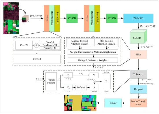
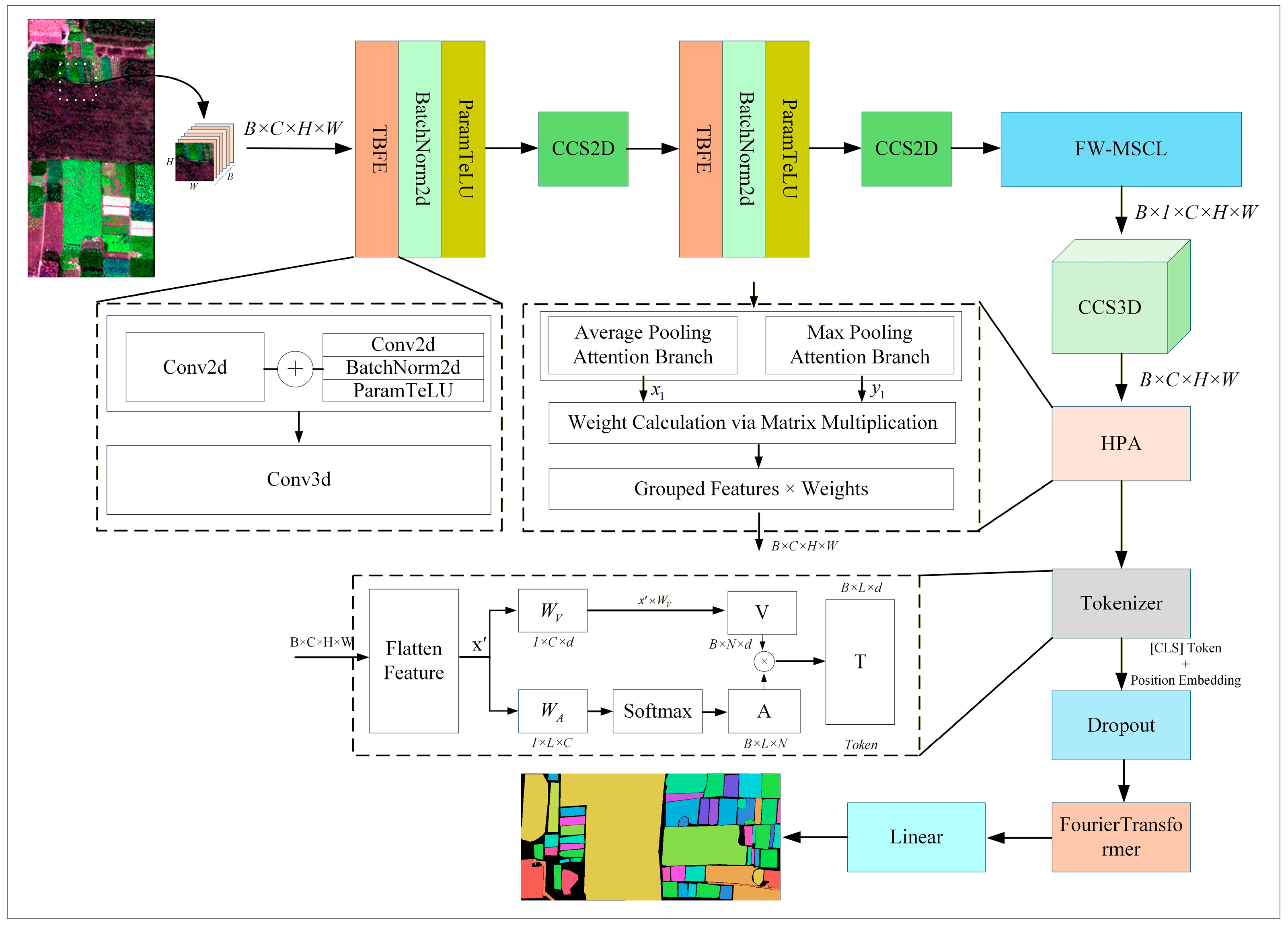
This paper proposes a hyperspectral data-based crop classification network. The overall architecture follows a processing pipeline that includes spectral–spatial feature extraction, feature enhancement via FW-MSCL, attention modulation, Transformer encoding, and discriminative classification. This design balances the inherent spatial–textural correlations and cross-scale structural information in hyperspectral imaging. The overall architecture diagram is shown in Figure 1.
Figure 1.
Overall model architecture.
In the network, a Tokenizer maps spatial features to the sequence input required by the Transformer. Here, WA denotes learnable parameters used to compute spatial position contribution weights, which help mitigate background noise interference. WV maps the original feature channels to the token dimension expected by the Transformer, enabling feature dimension adaptation. A represents the spatial token attention weights, and V denotes the dimension-adapted features.
During the feature extraction stage, the model employs a Two-Branch Feature Extractor (TBFE) to separately capture spectral correlations and spatial texture information, addressing the issue of crop spectral similarity. A CCS module is subsequently integrated to emphasize the most discriminative regions while reducing redundant information, alleviating generalization challenges caused by low sample size and refining feature representations for subsequent label prediction. The network further innovates with the FW-MSCL module, which enhances feature discriminability through multi-scale transformations and a nonlinear combination of wavelet basis functions. This module also incorporates a frequency space attention mechanism to strengthen interactions in the frequency domain, further improving noise suppression and discriminative capability.
For global modeling, the network adopts a Hybrid Positional Attention (HPA) mechanism combined with a Fourier-based Transformer encoder. HPA provides position-aware prior information, guiding the network to focus on row–column structural patterns and addressing global context dependencies. The Transformer efficiently captures long-range dependencies and periodic patterns through frequency domain self-attention while maintaining computational efficiency. Finally, a fully connected layer outputs class probabilities. Overall, the network improves hyperspectral image classification accuracy in complex scenes while maintaining computational efficiency and a modular, problem-oriented design.
2.2.2. Channel Cross-Spatial (CCS) Attention Mechanism
The Channel Cross-Spatial (CCS) module is a lightweight and robust attention mechanism designed to exploit the inherent spectral and spatial information in hyperspectral images. Different from traditional attention mechanisms that model channel and spatial features independently, the CCS module explicitly constructs a cross-modulation relationship between channel and spatial dimensions, thereby achieving adaptive refinement of spectral–spatial features for hyperspectral crop classification.
The operation of the CCS module follows a three-step pipeline: channel compression, spectral–spatial cross-interaction, and channel–spatial weighting. Two variants, namely CCS2D and CCS3D, are designed to adapt to different feature dimensions.
First, the module performs channel-wise global average pooling (implemented by the ChannelPool layer) on the input feature map X ∈ RB×C×H×W, where B denotes the batch size, C the number of channels, H and W the spatial height and width. This operation compresses multi-channel spectral features into a single-channel spatial response map M ∈ RB×1×H×W. It aggregates global spectral information into a compact spatial representation, suppresses background noise such as roofs, roads, and bare soil, and highlights spatial regions related to crops.
Convolution is then applied to the compressed response map M to model local spatial and spectral correlations. The kernel parameters of the two variants are defined as follows:
CCS2D operates on the 2D spatial domain (H, W) using a 3 × 3 convolution kernel to capture local spatial dependencies and enhance the spatial saliency of crop targets. CCS3D extends to the 3D spectral–spatial domain (C, H, W) using a 1 × 1 × 3 convolution kernel, which simultaneously models spectral correlations among adjacent bands and spatial correlations within local neighborhoods.
The convolved response map is activated by the Sigmoid function to generate attention weights α ∈ (0, 1), which are multiplied with the original input features X in a pixel-wise manner. This step realizes adaptive cross-modulation: discriminative channels and spatial locations relevant to crops are enhanced (high α values), while irrelevant background regions are suppressed (low α values).
By suppressing background noise and emphasizing discriminative channels and spatial positions, the CCS module provides more robust input features for subsequent modeling.
2.2.3. Fixed-Wavelet Multi-Scale Convolutional Layer
The FW-MSCL module draws inspiration from the Kolmogorov–Arnold Network (KAN) concept, employing a predefined wavelet function library as a set of basis functions combined with learnable linear combination weights to adaptively model nonlinear relationships. Wavelet transform can extract multi-scale spatial–spectral features and has demonstrated advantages in classification [40]. Kolmogorov–Arnold Networks (KAN) offer higher representational capacity than conventional MLPs in hyperspectral image classification tasks [41]. During training, these weight parameters are continuously updated, enabling the model to flexibly approximate more complex nonlinear mappings through weighted combinations of different basis functions. Consequently, this approach retains the desirable time–frequency properties of wavelets while gaining the ability to construct learnable nonlinear relations via basis function combinations. Moreover, by integrating grouped convolution-style weight design, feature reuse, and single-branch fusion, the module reduces the number of parameters, achieving a balance between computational efficiency and model robustness.
Specifically, we explicitly define the key implementation details of the FW-MSCL module as follows:
- (1)
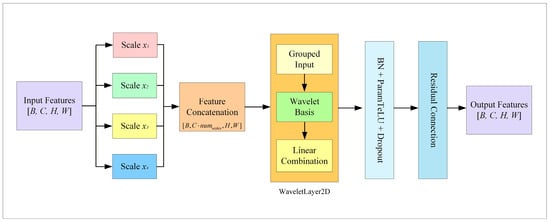
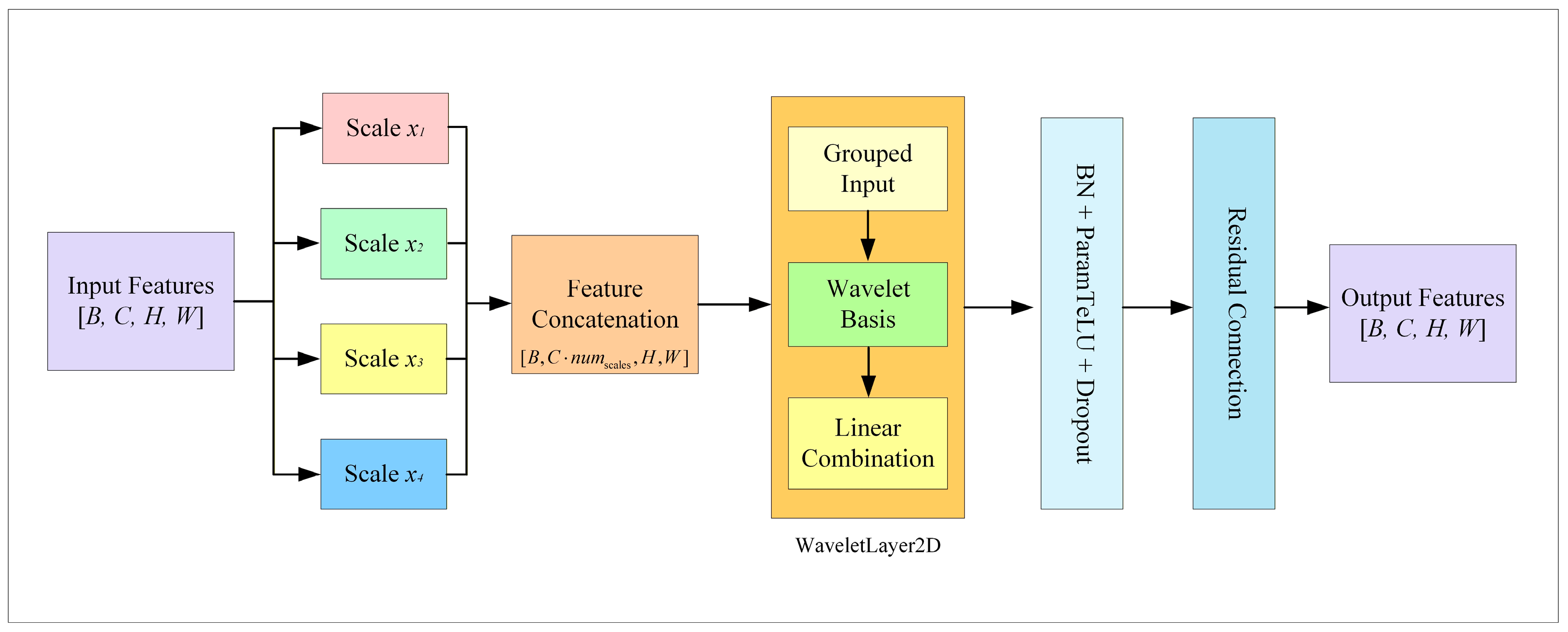
- Multi-scale feature generation: The input features (64 channels) are first scaled according to a preset set of scales (0.25, 1.5, 3.0, 4.0) to produce multi-scale feature representations. Each scaled feature retains the original channel count, while the amplitude transformation enhances the spectral–spatial representational capacity. These multi-scale features are then concatenated along the channel axis into a high-dimensional tensor.
- (2)
- Wavelet basis function discretization: Before nonlinear transformation, the input feature values of each scale are normalized to the interval [−3, 3] (covering the main response range of wavelet basis functions) and discretized via equidistant sampling with a step size of 0.01. This linear discretization strategy avoids numerical overflow while preserving the core characteristics of continuous wavelet functions.
- (3)
- Grouped multi-scale fusion: The concatenated high-dimensional tensor is processed by a WaveletKANLayer2D layer with a fixed group number of 8 (ensuring input and output channels are divisible by the group count). Each group applies a designated wavelet basis function for nonlinear transformation, and the outputs of all groups are aggregated via learnable linear weights. After fusion, the features are further refined through batch normalization and the ParamTeLU activation function, thereby enhancing gradient plasticity and nonlinear representational ability. A residual connection is finally added to fuse the refined multi-scale features with the original input features, preserving primary feature information. The architecture of the FW-MSCL module is shown in Figure 2.Figure 2. Architecture of the FW-MSCL module.
2.2.4. Fourier-Based Transformer Encoder
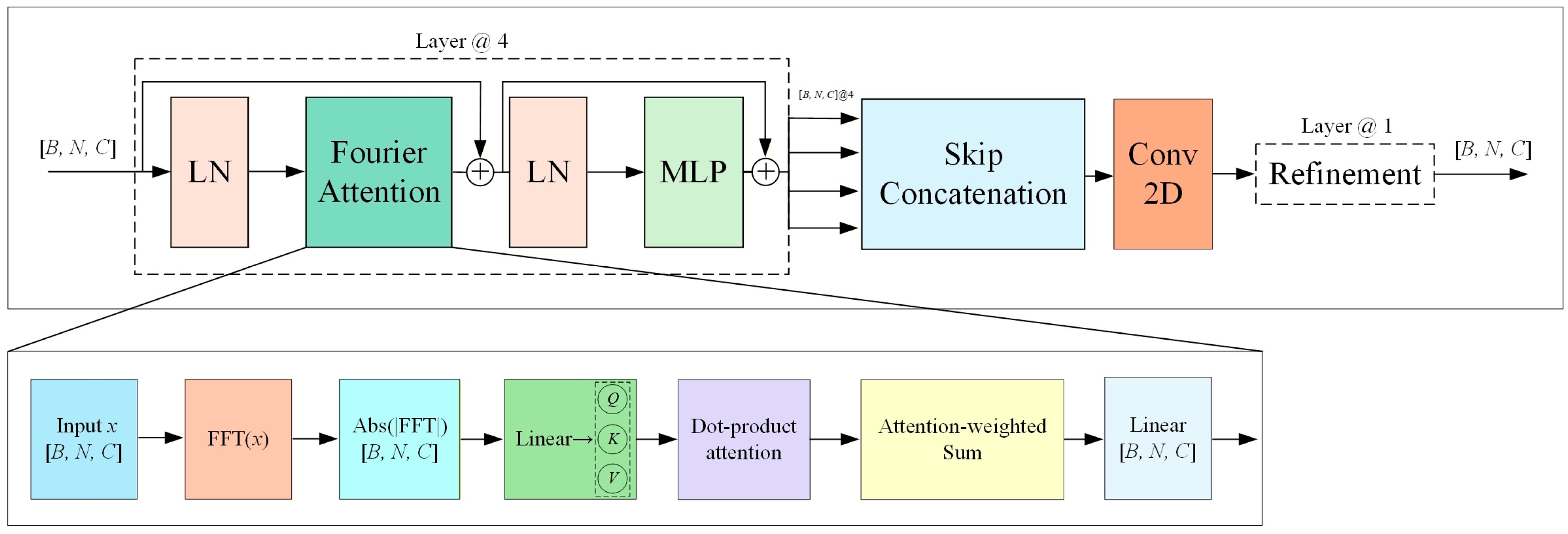
Li et al. demonstrated that the Fourier transform can be incorporated into neural networks to extract features in the frequency domain and improve the efficiency of hyperspectral image classification [42]. To extract frequency domain features from hyperspectral image sequences, this study designs a Fourier-based Transformer encoder. This module efficiently captures long-range dependencies and periodic patterns while maintaining computational efficiency. The core idea is to map the input sequence into the amplitude domain via a one-dimensional Fourier transform, thereby enhancing the frequency domain characteristics of the sequence. Multi-head self-attention is then applied to the transformed representation to achieve global pattern recognition.
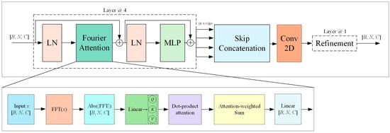
The encoder adopts a multi-layer stacked architecture, each layer containing two residual paths: one employs the Fourier Self-Attention (FSAT) module, and the other uses a Multi-Layer Perceptron (MLP) module. After Fourier analysis, the resulting amplitudes form the base tensors for queries (Q), keys (K), and values (V). Attention weights in the multi-head architecture are computed via scaled dot-product operations to capture patterns at different scales. Residual connections strengthen gradient propagation by linking the attention output with the input. Meanwhile, the MLP sub-layer consists of two fully connected layers combined with the ParamTeLU activation function and dropout, which improve nonlinear discriminative ability while preventing overfitting.
To facilitate information flow across encoder layers, a SkipCat cross-layer fusion strategy concatenates each layer’s output with the original input along an added dimension. Feature fusion and channel compression are achieved via two-dimensional convolution, ensuring efficient information transfer and reuse. The final output undergoes a second round of residual attention and MLP processing, yielding a serialized global feature representation for subsequent classification tasks. The structure of the Fourier-based Transformer encoder is illustrated in Figure 3.
Figure 3.
The structure of the Fourier-based transformer encoder.
2.2.5. Experimental Settings
The experiments were conducted on a workstation equipped with an NVIDIA RTX A4000 GPU, an Intel Xeon processor, and 128 GB of RAM, running on a Linux operating system. The implementation was developed in Python 3.10 within a Conda virtual environment. All DL experiments were performed using PyTorch 2.8.0, leveraging GPU acceleration and a set of common auxiliary libraries.
The model parameters were configured as follows. At the input stage, the hyperspectral data were first standardized, and PCA was applied to reduce the spectral dimension to 30 bands. The model accepts local patches of size 7 × 7 as input. The FW-MSCL operates with 64 input and output channels, employs four scaling factors (0.25, 1.5, 3.0, 4.0), uses the Morlet or DOG wavelet as the basis function, and adopts a grouping mechanism with 8 groups to reduce parameter count and computational complexity. The feature extraction stage combines the TBFE, the CCS module, and the Hybrid Positional Attention (HPA) module, with the learnable ParamTeLU serving as the activation function. For high-level semantic modeling, a Fourier-based Transformer is used, configured with an embedding dimension of 64, 4 layers, 16 attention heads, and an MLP hidden dimension of 8. During training, we set the learning rate to 0.01, weight decay to 0.01, momentum parameters to (0.9, 0.999), employed a StepLR scheduler, trained for 150 epochs, and used a batch size of 256.
To ensure proper model fitting and a fair comparison with baseline methods, an early stopping mechanism was applied during training. Specifically, training was terminated if the validation loss did not improve within a predefined number of epochs, preventing overfitting and ensuring that the baseline methods were trained under comparable conditions.
2.2.6. Evaluation Metric
Multiple quantitative metrics provided a comprehensive and unbiased assessment of classification efficacy. The evaluation metrics include Overall Accuracy (OA), Average Accuracy (AA), Kappa Coefficient, F1-Score, and Mean Intersection Over Union (MIoU). The evaluation of model efficiency is conducted through the trainable parameters and average prediction time per pixel. Thus, the model accuracy and computational performance are assessed together.
The OA serves as the main metric for assessing the precision of classification in hyperspectral remote sensing images. It represents the proportion of samples that are classified correctly compared to the total samples.
In this framework C indicates the total classes in hyperspectral remote sensing image. For each class i, TPi is equal to the number of instances correctly predicted to belongs to class i (True Positives) while FPi is equal to samples wrongly predicted to class i but actually belonging to other classes (False Positives). TNi is the number of samples not belonging to class i positively labeled as not belonging to class i (True Negatives) and FNi is number of samples which belong to class i but labeled as not belonging to class i (False Negatives).
The AA evaluation method is used to overcome OA’s weaknesses when data is imbalanced. First, the accuracy value of each class is calculated and then the average of these accuracies is taken. Using this methodology permits a more evenly distributed performance assessment of the model across all classes. The formula is calculated as follows:
A metric of fidelity, the Kappa coefficient (κ) is derived from the confusion matrix. It quantifies the alignment present between classifications rendered by a model and their corresponding ground-truth annotations. By its formulation it can be articulated as follows:
Within this discourse, denoted by Pe, expected accuracy contingent upon stochastic prognostication finds its computational representation articulated in subsequent fashion:
The Kappa coefficient ranges from −1 to 1. When κ = 1, the model’s predictions are fully consistent with the ground truth labels. When κ = 0, it indicates no difference exists between the model’s predictions and random guesses. when κ < 0, it signifies that the predictions are worse than random predictions.
As a fundamental evaluation metric in semantic segmentation and image classification, the MIoU measures the spatial accuracy of predictions for each category. The computation involves calculating the IoU between predicted labels and ground truth for every class, followed by averaging these values across all classes. This metric is especially important for assessing land cover classification performance in hyperspectral remote sensing applications. The corresponding calculation formulas are presented below.
First, calculate the IoU for the i-th class, denoted as IoUi:
Second, the MIoU is calculated as follows:
The F1-Score, which is the harmonic mean of precision and recall, is calculated as follows:
where
and
These metrics together offer a comprehensive evaluation of the model’s classification performance, both in terms of accuracy and computational efficiency.
3. Results
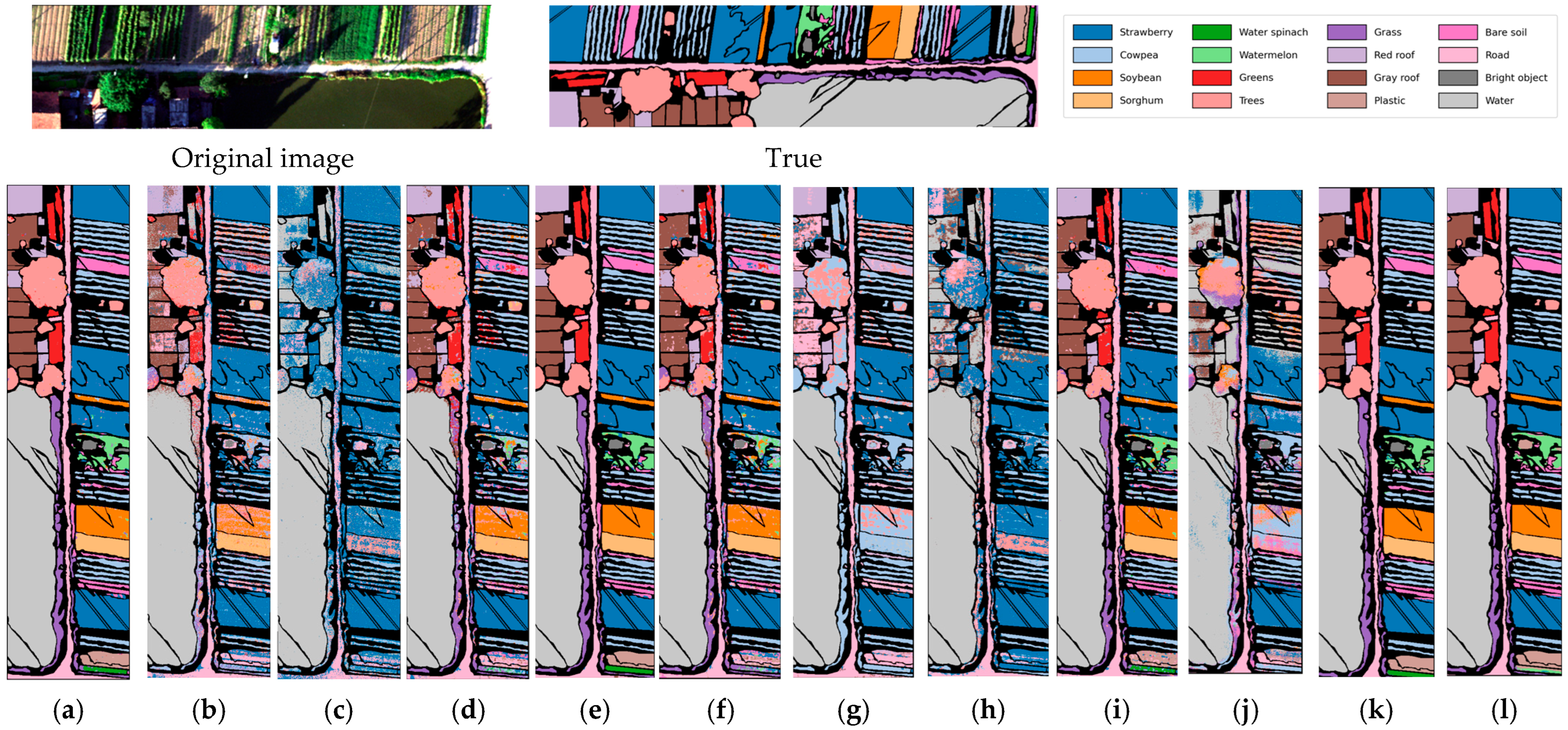
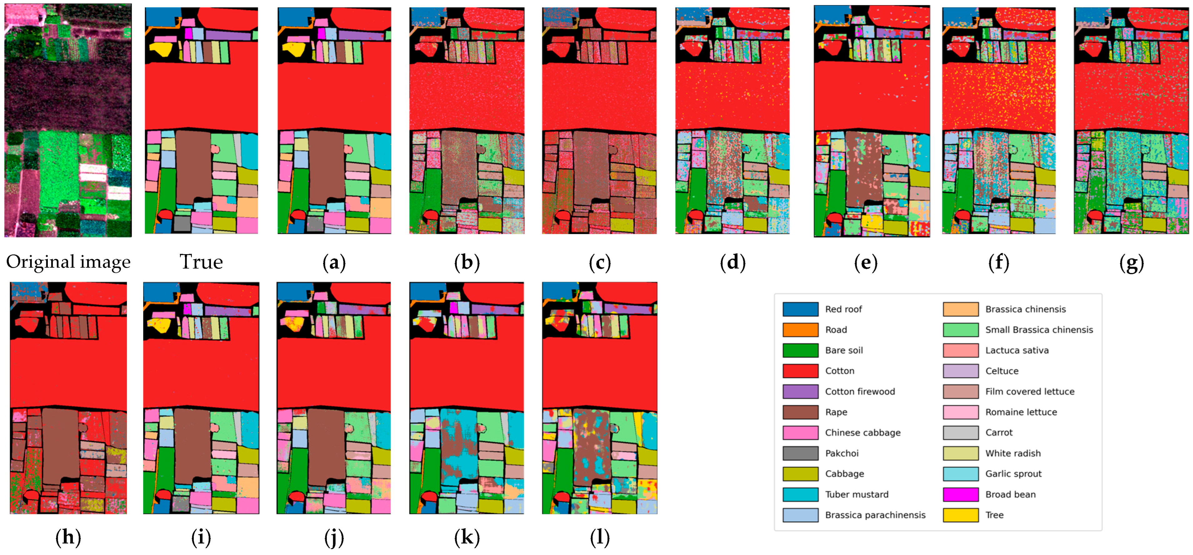
The original hyperspectral images depict real farmland scenes containing multiple crop types, while the ground truth masks accurately reflect the actual distribution of various crops and land cover features. To intuitively evaluate the performance of different models in hyperspectral crop classification, a qualitative comparison was conducted on both the HC and HH datasets, comparing the proposed method with several representative models, including Multi-Layer Perceptron (MLP), 1D-CNN [43], 3D-CNN [44], SSFTT [45], HybridSN [46], FreeNet [47], DGFNet [48], SCTNet [49], DSST [50], MDvT [51], and U-Net. The comparison revealed marked differences among the models in terms of field boundary preservation, class consistency, and the recognition performance for crops with limited samples.
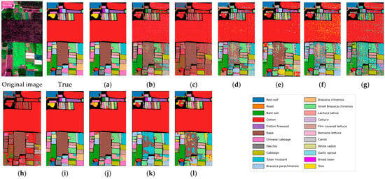
As shown in the visual comparison in Figure 4 and Figure 5, the proposed method demonstrates excellent performance, maintaining high spatial consistency while exhibiting strong spectral discriminative ability. It shows a good capability in distinguishing semantically similar and easily confused crop categories, such as “strawberry,” “cowpea,” and “soybean.” For instance, methods such as MLP, 1D-CNN, and DGFNet exhibit significant misclassifications in vegetation areas. Although 3D-CNN, HybridSN, FreeNet, and DSST show some improvement in spatial details, they still introduce noticeable noise in heterogeneous regions. While SSFTT, SCTNet, DSST, MDvT, and U-Net outperform other models in preserving structural information, they still display obvious classification errors in small patch areas.
Figure 4.
Classification results of different methods on the HC dataset. (a) MSWKN; (b) 1D-CNN; (c) MLP; (d) 3D-CNN; (e) SSFTT; (f) HybridSN; (g) FreeNet; (h) DGFNet; (i) SCTNet; (j) DSST; (k) MDvT; (l) UNet.
Figure 5.
Classification results of different methods on the HH dataset. (a) MSWKN; (b) 1D-CNN; (c) MLP; (d) 3D-CNN; (e) SSFTT; (f) HybridSN; (g) FreeNet; (h) DGFNet; (i) SCTNet; (j) DSST; (k) MDvT; (l) UNet.
To objectively evaluate the proposed method, this paper conducts a comprehensive quantitative comparison with current state-of-the-art methods. To ensure the reliability and stability of the experimental results, all experiments are repeated five times with different fixed random seeds, and the final results are presented in the form of mean ± standard deviation. The evaluation covers multiple dimensions: class-wise accuracy, Overall Accuracy (OA), Kappa coefficient, F1-Score, Mean Intersection over Union (MIoU), and training time, so as to achieve a balanced and comprehensive assessment.
As shown in Table 3, MSWKN achieves superior overall classification performance on the HC dataset. It achieves an OA of 96.32% with a standard deviation within 0.08%, demonstrating high stability. Its AA is 95.35% with a standard deviation of 0.23%, and the Kappa coefficient reaches 95.71%, which also reflects excellent class balance and classification consistency. In addition, MSWKN obtains a mIoU of 87.54% with a standard deviation of only 0.41%, further verifying the superiority of the model in spatial prediction accuracy.
Table 3.
Performance Comparison of Different Models on the HC Dataset.
In terms of the classification results of major crop types, MSWKN achieves relatively high accuracy on classes such as strawberry, cowpea, soybean, sorghum, and water spinach. Specifically, the classification accuracy of strawberry (Class 1) reaches 97.20%, and that of sorghum (Class 4) is 97.78%, with the standard deviations of both classes controlled below 0.15%, which demonstrates the model’s strong feature extraction capability. For classes with a small number of samples and scattered spatial distribution, such as water spinach and watermelon, the proposed model achieves relatively lower accuracy. In comparison, traditional models including MLP and 1D-CNN present significantly lower accuracy and larger standard deviations on water spinach, watermelon, and other classes, indicating that they struggle to distinguish crops with subtle spectral differences.
To further verify the generalization ability of the MSWKN model in fine-grained multi-crop classification tasks, experiments were conducted on the HH hyperspectral crop dataset. This dataset includes various typical crop classes such as cotton, rape, Chinese cabbage, and pakchoi, and some crops have high spectral similarity, which increases the difficulty of classification. As shown in Table 4, MSWKN also outperforms other comparative methods on the HH dataset, achieving an OA of 97.78%, an AA of 96.99%, a Kappa coefficient of 97.33%, and a MIoU of 91.15%, with all indicators showing good performance.
Table 4.
Performance Comparison of Different Models on the HH Dataset.
In terms of major crop identification, MSWKN achieves classification accuracies of over 95% for frequently occurring crops such as cotton, rape, Chinese cabbage, and pakchoi. Specifically, the accuracy for cotton reaches 98.67% (standard deviation: 0.06%), and that for rape is 99.52% (standard deviation: 0.24%), indicating that the model can adequately capture spectral and spatial characteristics of crops and effectively reduce confusion between different crop types. However, for classes with small planting areas and scattered distributions such as pakchoi, the performance of the proposed model is slightly lower than that of SSFTT. For other crops such as lettuce, romaine lettuce, and broad bean, MSWKN exhibits strong recognition ability, with classification accuracies of 95.25%, 99.66%, and 97.96%, respectively. These results are superior to those obtained by traditional methods including 1D-CNN and MLP, which generally suffer from low accuracy and large standard deviations. This demonstrates that MSWKN has a certain robustness advantage in crop classification tasks.
In summary, the proposed method outperforms all comparison methods on both datasets and achieves excellent performance in crop type recognition. Most categories achieve high accuracy, with the standard deviations generally controlled at a low level, and no complete misclassification occurs for any category. Although the proposed method exhibits favorable performance on these two datasets, its performance on data with different spatial resolutions and sensors needs further discussion. Therefore, this section analyzes the performance of the proposed method on data with different spatial resolutions and sensors in Section 4, and introduces three additional datasets with different spatial resolutions.
4. Discussion
4.1. Comparison of t-SNE Feature Visualization
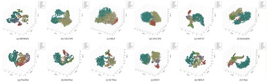
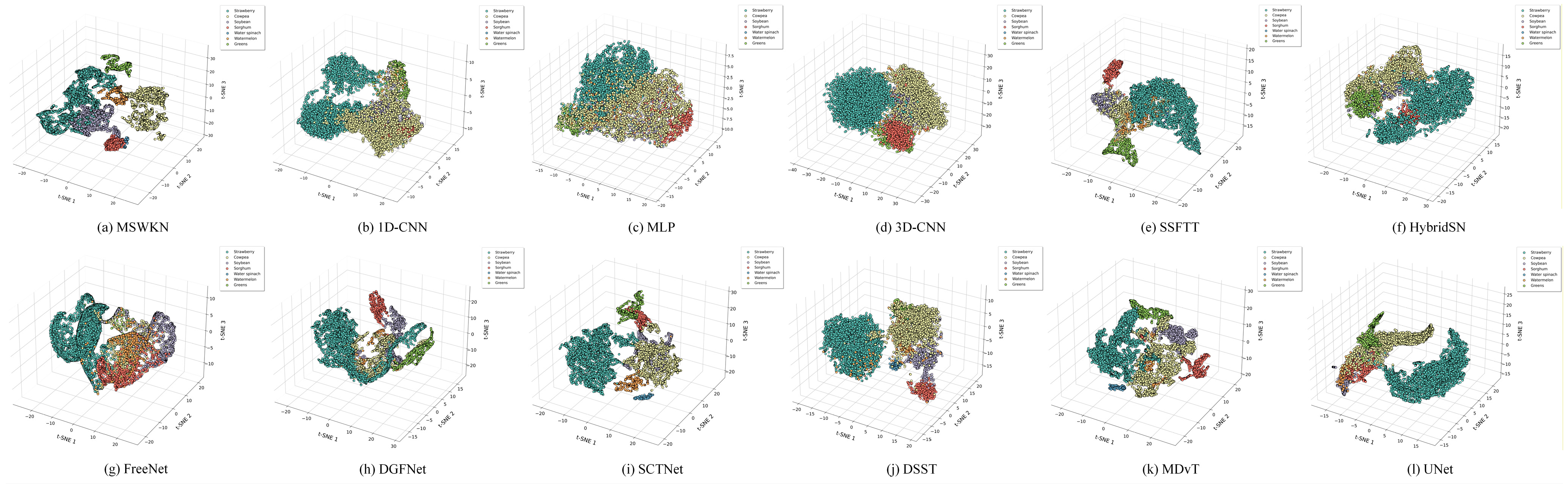
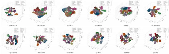
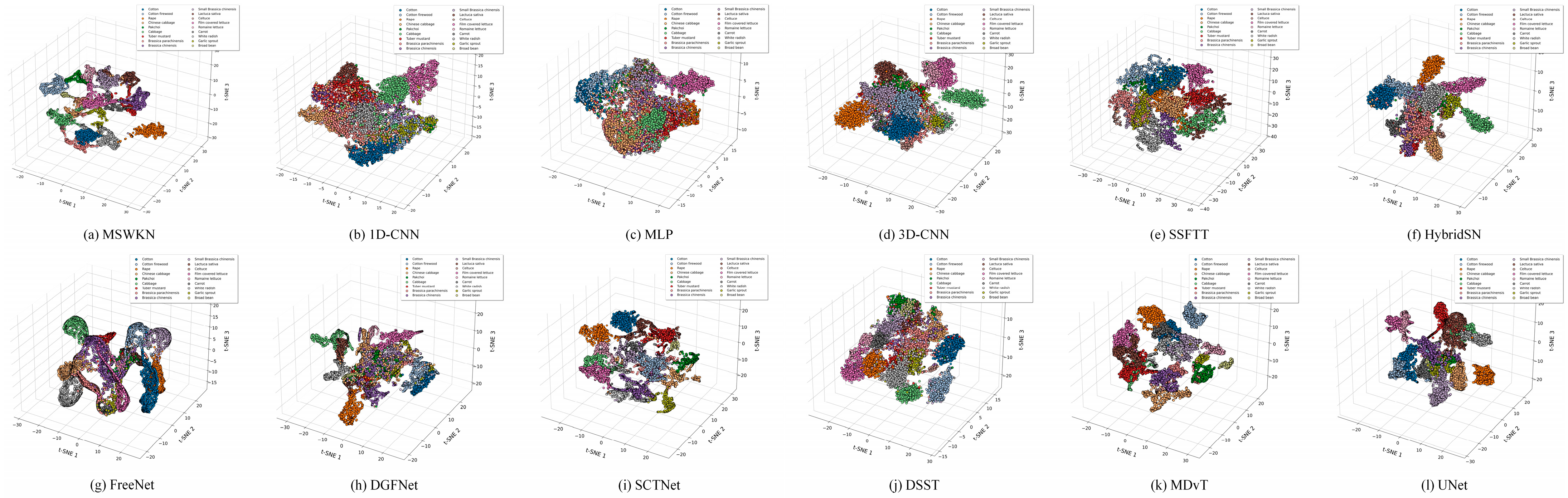
To further explain why the proposed model can improve classification accuracy and intuitively evaluate the feature separability of different hyperspectral crop classification models, this section conducts a t-SNE dimensionality reduction visualization analysis on the deep features extracted by each model. We select crop categories from both the HC and HH hyperspectral datasets, and compare the proposed MSWKN model with several baseline models. The visualization results are shown in Figure 6 (for the HC dataset) and Figure 7 (for the HH dataset), where different colors represent different crop classes. The compactness of the spatial distribution of feature points and the degree of separation between classes directly reflect the discriminative ability of the learned features.
Figure 6.
t-SNE visualization of the embedded features learned by different methods on the HC dataset. Different colors represent different crop classes.
Figure 7.
t-SNE visualization of the embedded features learned by different methods on the HH dataset. Different colors represent different crop classes.
The proposed MSWKN model exhibits the most discriminative feature distributions on both datasets. As shown in Figure 6a and Figure 7a, the embedded features learned by MSWKN form relatively compact intra-class clusters and clearly separated inter-class boundaries in the low-dimensional space. This explains, at the feature level, why MSWKN achieves high accuracy in the classification tasks. In contrast, the performance of other compared methods shows various limitations. For instance, the features extracted by MLP, 1D-CNN, and 3D-CNN exhibit relatively loose intra-class aggregation and notable overlapping regions between classes, indicating their limited ability to capture subtle feature differences in hyperspectral crops. Although HybridSN and SSFTT models show improved feature separability, their inter-class margins remain less distinct than those of MSWKN.
The analysis indicates that the MSWKN model is capable of learning highly discriminative deep representations. It effectively maps samples of the same class to compact regions in the embedded space while pushing apart samples from different classes, thereby achieving superior inter-class separability at the feature level.
4.2. Model Efficiency Evaluation
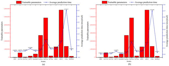
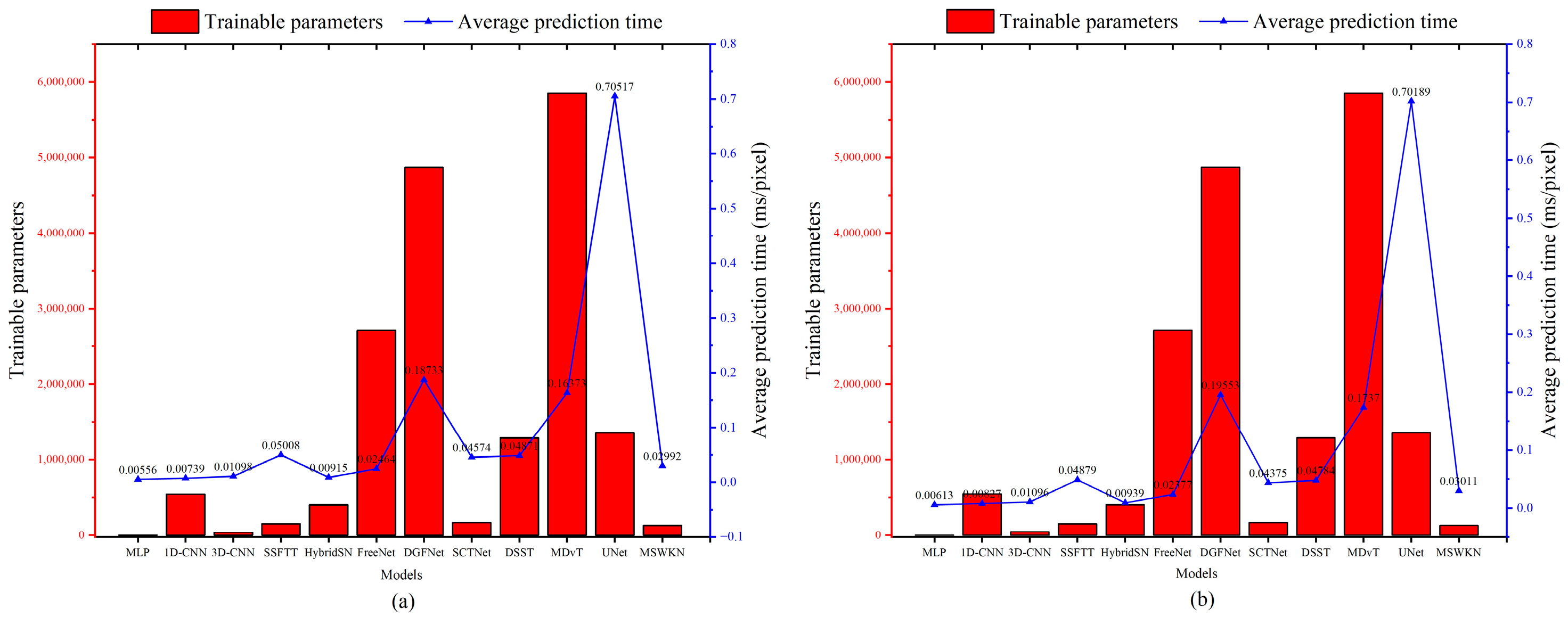
In this section, we evaluate the computational efficiency of the proposed model in terms of the number of trainable parameters, average per-pixel prediction latency, and training time, as illustrated in Figure 8a,b, and Table 5. All experiments are conducted in a unified hardware environment on a workstation equipped with an NVIDIA RTX A4000 GPU, an Intel Xeon processor, and 128 GB of RAM, running the Linux operating system. The batch size is set to 256 during inference. The average per-pixel prediction latency is defined as the average prediction time per sample over the entire dataset. The training time is obtained as the average value of five independent training runs with different random seeds. All comparative methods are implemented under the same hardware and experimental settings to ensure a fair comparison.
Figure 8.
Relationship between model complexity and inference speed on different datasets. (a) HC dataset, (b) HH dataset.
Table 5.
Comparison of Training Time for Different Models.
On the HC dataset, the MSWKN method requires only 133,258 parameters, which is substantially fewer than most comparative methods. This represents a reduction of 91.3% compared to SCTNet (168,009 parameters), 89.6% compared to SSFTT (153,217 parameters), and 99.0% compared to U-Net (1,357,169 parameters). In terms of inference efficiency, our method achieves a per-pixel prediction time of 0.02992 ms, outperforming SSFTT (0.05008 ms/pixel), SCTNet (0.04574 ms/pixel), and DSST (0.04871 ms/pixel). These results demonstrate the method’s ability to deliver fast predictions while maintaining high accuracy, achieving a favorable trade-off between computational cost and model performance. A similar trend is observed on the HH dataset, where the method maintains its efficiency advantage with 133,648 trainable parameters and an average prediction time of 0.03836 ms per pixel.
Table 5 quantitatively compares the training time of different models. On both the HC and HH datasets, the proposed MSWKN method achieves relatively short training durations, which are 138.44 s and 199.58 s, respectively. In terms of training efficiency, MSWKN significantly outperforms SCTNet and SSFTT on both datasets. Although the training time of MSWKN is slightly higher than that of lightweight models such as MLP, its classification accuracy is substantially superior to MLP and other comparative methods. In summary, the proposed method exhibits outstanding computational efficiency while preserving excellent classification accuracy.
4.3. Performance Comparison of Different Models Under Varying Training Data Sizes
To further evaluate the robustness of the proposed method under limited training data conditions, additional experiments were conducted using different proportions of training samples. In hyperspectral image classification, the acquisition of labeled samples is often expensive and time-consuming, making it essential to investigate how model performance varies as the amount of available training data decreases. Therefore, by gradually adjusting the training sample ratios, we analyze the robustness of different models to training data reduction.
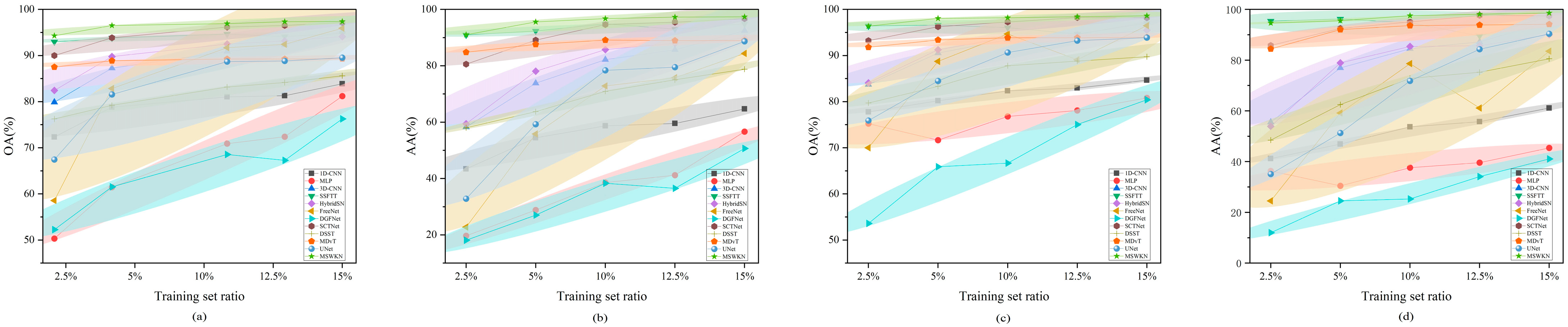
As shown in Figure 9, the classification performance of different methods under varying training sample ratios is presented. The overall accuracy (OA) and average accuracy (AA) curves indicate that most models exhibit gradual performance improvements as the number of training samples increases. When the training data is limited, traditional models such as MLP and 1D-CNN show relatively poor performance, indicating that their purely spectral feature extraction strategies suffer from limited generalization capability when labeled samples are scarce. In contrast, more advanced models such as SSFTT, SCTNet, and the proposed MSWKN maintain relatively stable performance across different training sample ratios.
Figure 9.
Comparison of overall accuracy and average accuracy of different models under varying training sample ratios. (a) Overall accuracy on the HC dataset, (b) Average accuracy on the HC dataset, (c) Overall accuracy on the HH dataset, (d) Average accuracy on the HH dataset.
Specifically, when the training sample ratio is reduced to 2.5%, the proposed MSWKN achieves an OA of 94.29% on the HC dataset and 96.36% on the HH dataset, with corresponding AA values of 91.01% and 94.63%, respectively. These results outperform all other comparative methods under the same training conditions, demonstrating the strong capability of the proposed model to extract discriminative spectral–spatial features even with limited training samples.
Furthermore, the performance curve of MSWKN remains relatively smooth as the training sample ratio decreases, indicating smaller performance degradation compared with other models. This suggests that the proposed method exhibits strong robustness to training data reduction and reduced dependence on large-scale labeled datasets. Consequently, the proposed model shows promising potential for practical hyperspectral image classification scenarios where labeled samples are limited.
4.4. Wavelet Kernel Selection
To evaluate the influence of wavelet kernel selection on model performance, each wavelet kernel was run five times with different random seeds, and the mean values of the results are reported in Table 6. On the HC dataset, the Morlet wavelet kernel achieved relatively better average performance among all the tested kernels. Its OA, AA, Kappa coefficient, F1-score, and MIoU were 96.32%, 95.35%, 95.71%, 97.35%, and 87.54%, respectively. The Mexican Hat, DOG, and Gaussian kernels produced comparable results, with only small differences across all evaluation metrics. In contrast, the Haar kernel achieved relatively lower performance.
Table 6.
Performance Comparison of Different Wavelet Kernels.
On the HH dataset, the DOG kernel obtained relatively higher OA and MIoU, while the Symmetric Mexican kernel also achieved competitive results. Overall, the differences between most wavelet kernels were relatively small, indicating that model performance is not highly sensitive to the specific choice of wavelet kernel.
The experimental results show that the Morlet and DOG kernels achieved good performance on both datasets. However, the differences between most kernels were small, suggesting that the selection of wavelet kernel has a limited impact on model performance.
4.5. Model Performance Under Different Spatial Resolutions
Although the proposed method exhibits excellent performance on the WHU-Hi series datasets (HC and HH), both datasets were acquired using the same hyperspectral imaging system with highly consistent collection conditions. Therefore, the experimental validation of this study has certain limitations in terms of dataset diversity. To further evaluate the adaptability and generalization ability of the proposed method, this section conducts experiments on hyperspectral remote sensing image classification using datasets with different spatial resolutions and sensor types, and analyzes the performance of the proposed method on these additional datasets. The datasets used include the WHU-Hi-LongKou, Indian Pines, and Salinas datasets. Detailed information of each dataset is provided below. The WHU-Hi-LongKou dataset has a spatial resolution of 0.463 m and was acquired by the Headwall Nano-Hyperspec sensor (Headwall Photonics, Inc., Bolton, MA, USA). It covers the visible to near-infrared spectral range (400–1000 nm) with approximately 270 bands, featuring high spatial and spectral resolution. The Indian Pines dataset has a spatial resolution of 3.7 m and was collected by the AVIRIS sensor (NASA Jet Propulsion Laboratory, Pasadena, CA, USA), developed by the NASA Jet Propulsion Laboratory. It covers a spectral range of 400–2500 nm and contains 224 bands in total, among which 200 bands are commonly used after noise removal. The Salinas dataset also has a spatial resolution of 3.7 m and was acquired by the AVIRIS sensor. Covering the Salinas Valley in California, USA, this dataset contains 224 bands and consists of 16 ground categories, including vegetables, bare soil, and vineyards.
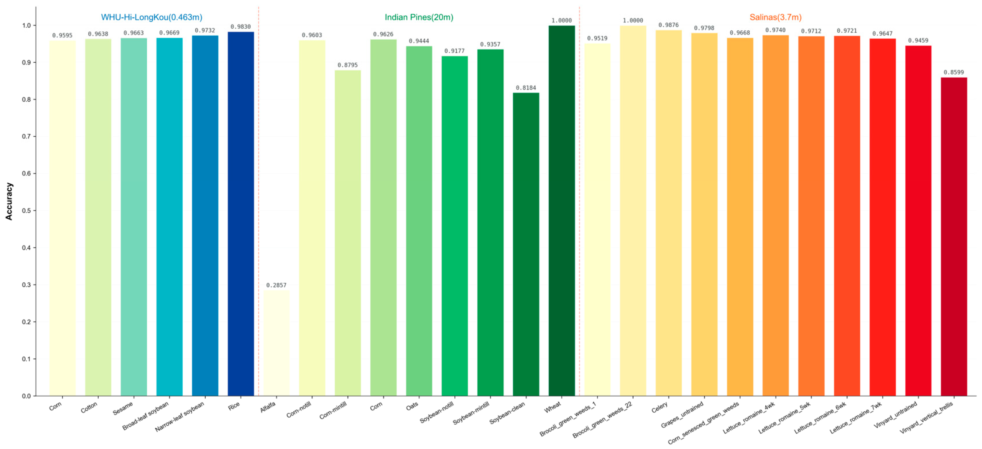
The results in Figure 10 indicate that the crop classification performance of the MSWKN model varies across datasets with different spatial resolutions. For the high spatial resolution dataset (0.463 m), the model is able to capture fine spatial details and texture differences of crops, achieving high classification accuracy. For instance, the classification accuracies of broad-leaf soybean and narrow-leaf soybean both exceed 96%, demonstrating strong discriminative capability. For the medium spatial resolution dataset (3.7 m), most crops achieve accuracies above 95%, with only the Vinyard vertical trellis class having an accuracy below 90%. In contrast, the low spatial resolution dataset (20 m) negatively impacts the model’s performance, with the accuracy of the Alfalfa class being only 28.57%, while most other classes still achieve accuracies above 90%.
Figure 10.
Crop classification performance of the model under different spatial resolutions.
The results show that although datasets with different spatial resolutions and sensors were used for validation, and the MSWKN model exhibits excellent performance on high-spatial-resolution datasets, it should be noted that the overall scale and diversity of the datasets remain limited, and they do not cover all crop types and geographical regions. In addition, the classification accuracy of some categories (e.g., alfalfa) decreases significantly at low spatial resolutions, indicating that high-resolution spatial information remains indispensable for the recognition of specific crop types. Future research will extend validation to more datasets acquired from diverse sensors, geographical regions, and a wider range of crop types, so as to comprehensively evaluate the robustness and generalization ability of the proposed model.
4.6. Ablation Study
To evaluate the contribution of each component to the overall performance of the proposed model, ablation experiments were conducted on the WHU Hi HanChuan (HC) and WHU Hi HongHu (HH) datasets. In these experiments, the following modules were progressively introduced or removed: TBFE, CCS, HPA, FSAT, and FW-MSCL, and their effects on classification accuracy, model parameter scale, and inference efficiency were analyzed.
On the HC dataset (Table 7), introducing the TBFE module improves the OA to 95.51% and the MIoU to 84.84%, indicating that spatiotemporal feature extraction plays an important role in enhancing model performance. Meanwhile, the number of trainable parameters increases from 61,469 to 130,923, and the inference time rises from 0.0081 ms per pixel to 0.0185 ms per pixel, suggesting that the improved feature representation capability introduces additional computational overhead. After further incorporating the CCS module, OA increases to 96.08% and MIoU to 86.38%. The number of parameters changes only slightly, while the inference time increases marginally to 0.0234 ms per pixel, indicating that this module effectively improves classification performance while maintaining relatively low model complexity. With the addition of the HPA module, OA and MIoU reach 96.12% and 86.85%, corresponding to improvements of 0.04% and 0.47%, respectively. At this stage, the number of parameters increases to 131,016, and the inference time becomes 0.0264 ms per pixel. After further integrating the FSAT module, OA and MIoU increase to 96.21% and 86.94%, respectively. The parameter scale remains unchanged, while the inference time slightly increases to 0.0274 ms per pixel. Finally, after integrating the FW-MSCL module, OA and MIoU reach 96.51% and 87.28%, representing further improvements of 0.30% and 0.34% compared with the previous configuration. Meanwhile, the number of model parameters increases slightly to 133,258, and the inference time becomes 0.0299 ms per pixel. Overall, while introducing only a limited increase in parameters, FW-MSCL significantly improves classification accuracy and maintains efficient computational performance, demonstrating its effectiveness in lightweight multi-scale feature modeling.
Table 7.
Ablation Analysis of Module Contributions on the HC Dataset. (√: module included; ×: module excluded.).
On the HH dataset (Table 8), introducing the TBFE module increases the OA to 97.54% and the MIoU to 89.67%. Meanwhile, the number of model parameters increases to 131,313, and the inference time rises to 0.0224 ms per pixel.
Table 8.
Ablation Analysis of Module Contributions on the HH Dataset. (√: module included; ×: module excluded.).
Subsequently, the CCS, HPA, and FSAT modules are progressively incorporated. As a result, the OA values change to 97.71%, 97.62%, and 97.45%, while the MIoU values reach 90.41%, 90.06%, and 89.31%, respectively. During this process, the parameter scale changes only slightly (from 131,313 to 131,406), whereas the inference time exhibits a modest increase (from 0.0224 ms per pixel to 0.0280 ms per pixel), indicating that these modules attempt to enhance feature representation while maintaining relatively low model complexity, with minor fluctuations in performance after partial module integration.
After integrating the FW-MSCL module, the OA and MIoU further improve to 97.88% and 91.15%, corresponding to increases of 0.43% and 1.84%, respectively, compared with the performance after incorporating the FSAT module. At the same time, the number of model parameters increases to 133,648, and the inference time becomes 0.0301 ms per pixel. Although the parameter scale increases slightly, the resulting accuracy improvement is more substantial. These results demonstrate that the FW-MSCL module can effectively improve model performance while maintaining high computational efficiency, thereby verifying its effectiveness in lightweight network architecture design.
4.7. Hyperparameter Sensitivity Analysis
The performance of deep learning models is often influenced by the choice of hyperparameters. To validate the rationality of key hyperparameter settings in the proposed MSWKN model and to investigate their impact on classification performance, this section conducts systematic sensitivity analysis experiments on the HC dataset. The experiments employ a controlled variable approach, where only one parameter is varied at a time while keeping others at their default values (30 PCA components, 7 × 7 spatial patch, 4 scales, 8 groups, and 16 attention heads), with OA, AA, F1-score, and MIoU used as evaluation metrics.
PCA is employed to reduce the spectral dimensionality of hyperspectral data, where the number of retained components directly affects information integrity and computational complexity. As shown in Table 9, when PCA components increase from 20 to 30, OA improves from 96.30% to 96.32%; although AA slightly decreases, both OA and F1-score show improvement. However, when components further increase to 40 and 50, OA slightly decreases, possibly due to noise introduced by excessive components. The input patch size determines the spatial context available for feature extraction. Table 9 demonstrates that the small 3 × 3 patch fails to capture sufficient spatial neighborhood information, resulting in poor model performance, while the 5 × 5 patch substantially improves OA, and the 7 × 7 patch achieves optimal performance. Regarding the multi-scale feature extraction strategy adopted by MSWKN, increasing scales from 3 to 4 improves model performance. As for the grouping mechanism, when the group number is set to 8, the model achieves relatively good OA of 96.32%, whereas excessive grouping may cause feature fragmentation and degrade performance. With 16 attention heads, OA reaches 96.32%; further increasing heads yields comparable performance but increases computational complexity. In summary, all key hyperparameters adopted in MSWKN have been empirically validated as reasonable choices under the current dataset and model architecture, providing reference insights for hyperparameter settings in related research.
Table 9.
Hyperparameter sensitivity analysis results of the MSWKN model on the HC dataset.
5. Conclusions
This study proposes a deep neural network for crop classification based on hyperspectral images. The network integrates a FW-MSCL, a CCS attention mechanism, and a Fourier-based self-attention mechanism to achieve high-precision and efficient crop classification. Experimental results show that the proposed model achieves excellent performance on the WHU-Hi dataset in terms of OA, AA, F1-score, and mIoU. Ablation experiments verify the effectiveness of each module. Specifically, the combination of the FW-MSCL and Fourier self-attention enhances feature discriminability, while the CCS module strengthens global context modeling through joint spectral–spatial optimization. By adopting grouped convolutions, the FW-MSCL reduces the number of parameters without reducing model robustness, thereby ensuring high computational efficiency and fast inference speed. In addition, this study validates the advantages of the Morlet and DOG wavelet kernels for spectral feature extraction, highlighting the importance of wavelet kernel selection for model performance. However, the experiments in this study are mainly validated on specific public benchmark datasets, and the generalization ability of the model in more diverse and complex scenarios needs to be further verified. Furthermore, the performance of the proposed method under low spatial resolution remains unstable, and further optimization is required to improve its stability under low-resolution conditions. Overall, the proposed framework provides an accurate and efficient solution for hyperspectral crop classification and exhibits broad application potential in precision agriculture, crop growth monitoring, and automatic land use mapping. Future work will focus on addressing the above limitations to further enhance the robustness and generalizability of the method.
Author Contributions
Conceptualization, Z.L. and W.Z.; Methodology, Z.L. and W.Z.; Validation, W.Z., B.L. and B.Z.; Data curation, Z.L., B.L. and B.Z.; Writing—Original Draft Preparation, Z.L. and W.Z.; Writing—review and editing, Z.L., Z.X., J.G., N.L. and W.L.; Visualization, Z.L., W.Z. and B.L.; Software, W.Z. and W.L.; Funding acquisition, Z.L. and J.G. All authors have read and agreed to the published version of the manuscript.
Funding
This work was supported in part by the Henan Science and Technology R&D Program (Joint Funds Project) under Grant No. 242103810017, in part by the Joint Fund of Collaborative Innovation Center of Geo-Information Technology for Smart Central Plains, Henan Province and Key Laboratory of Spatiotemporal Perception and Intelligent Processing, Ministry of Natural Resources under Grant No. 231103 and the Open Fund of State Key Laboratory of Spatial Datum under Grant No. SKLGIE2024-Z-4-1 and SKLGIE2024-ZZ-8.
Institutional Review Board Statement
Not applicable.
Data Availability Statement
The original contributions presented in this study are included in the article. The code supporting the conclusions of this research is publicly available at https://github.com/wllnHUOT/MSWKN.git (accessed on 13 March 2026). Further inquiries can be directed to the corresponding authors.
Conflicts of Interest
The authors declare no conflicts of interest.
References
- Yan, Y.; Dang, C.; Liu, L.; Wang, Z.; Chen, L.; Jin, Z.; Kuzyakov, Y.; Chen, J.M.; Zhou, F.; Zhou, Y.; et al. Clumped canopy architecture raises global crop yield and reduces N2O emissions. Nat. Plants 2026, 12, 49–61. [Google Scholar] [CrossRef] [Scilit]
- Chen, X.; Ma, C.; Zhou, H.; Liu, Y.; Huang, X.; Wang, M.; Cai, Y.; Su, D.; Muneer, M.A.; Guo, M.; et al. Identifying the main crops and key factors determining the carbon footprint of crop production in China, 2001–2018. Resour. Conserv. Recy. 2021, 172, 105661. [Google Scholar] [CrossRef] [Scilit]
- Tang, Y.; Sun, S.; Lei, Y.; Mo, F.; Zhao, J.; Li, C.; Tong, J.; Wang, Y. Assessing the impact of climate and crop diversity on regional greenhouse gas emissions and water demand of cropland. Agr. Forest Meteorol. 2024, 355, 110119. [Google Scholar] [CrossRef] [Scilit]
- Song, J.; Liu, Y.; Zhuang, M.; Gu, W.; Cui, Z.; Pang, M.; Yang, Y. Estimating crop carbon footprint and associated uncertainty at prefecture-level city scale in China. Resour. Conserv. Recy. 2023, 199, 107263. [Google Scholar] [CrossRef] [Scilit]
- Liu, Y.; Diao, C.; Yang, Z.; Mei, W.; Guo, T. A novel Normalized Harvest Phenology Index (NHPI) for corn and soybean harvesting date detection using Landsat and Sentinel-2 imagery on Google Earth Engine. Remote Sens. Environ. 2025, 331, 115016. [Google Scholar] [CrossRef] [Scilit]
- Zhang, Y.; Gao, J.; Cen, H.; Lu, Y.; Yu, X.; He, Y.; Pieters, J.G. Automated spectral feature extraction from hyperspectral images to differentiate weedy rice and barnyard grass from a rice crop. Comput. Electron. Agr. 2019, 159, 42–49. [Google Scholar] [CrossRef] [Scilit]
- Wang, L.; Wang, J.; Liu, Z.; Zhu, J.; Qin, F. Evaluation of a deep-learning model for multispectral remote sensing of land use and crop classification. Crop J. 2022, 10, 1435–1451. [Google Scholar] [CrossRef] [Scilit]
- Shuai, L.; Li, Z.; Chen, Z.; Luo, D.; Mu, J. A research review on deep learning combined with hyperspectral Imaging in multiscale agricultural sensing. Comput. Electron. Agr. 2023, 217, 108577. [Google Scholar] [CrossRef] [Scilit]
- Jiang, N.; Geng, S.; Zheng, Y.; Sun, L. MSDCA: A Multi-Scale Dual-Branch Network with Enhanced Cross-Attention for Hyperspectral Image Classification. Remote Sens. 2025, 17, 2198. [Google Scholar] [CrossRef] [Scilit]
- Farmonov, N.; Amankulova, K.; Szatmári, J.; Sharifi, A.; Abbasi-Moghadam, D.; Nejad, S.M.M.; Mucsi, L. Crop type classification by DESIS hyperspectral imagery and machine learning algorithms. IEEE J. Sel. Topics Appl. Earth Observ. Remote Sens. 2023, 16, 1576–1588. [Google Scholar] [CrossRef] [Scilit]
- Xie, J.; Hua, J.; Chen, S.; Wu, P.; Gao, P.; Sun, D.; Lyu, Z.; Lyu, S.; Xue, X.; Lu, J. HyperSFormer: A transformer-based end-to-end hyperspectral image classification method for crop classification. Remote Sens. 2023, 15, 3491. [Google Scholar] [CrossRef] [Scilit]
- Khan, A.; Vibhute, A.D.; Mali, S.; Patil, C.H. A systematic review on hyperspectral imaging technology with a machine and deep learning methodology for agricultural applications. Ecol. Inform. 2022, 69, 101678. [Google Scholar] [CrossRef] [Scilit]
- Chen, J.; Li, W.; El-Askary, H. Spectral-Spatial Transformer with Multi-Scale Convolutional Attention for Hyperspectral Image Classification. IEEE J. Sel. Topics Appl. Earth Observ. Remote Sens. 2025, 18, 24223–24241. [Google Scholar] [CrossRef] [Scilit]
- Li, Y.; Zhang, L.; Chen, L.; Ma, Y. Superpixel guided spectral-spatial feature extraction and weighted feature fusion for hyperspectral image classification with limited training samples. Sci. Rep. 2025, 15, 3473. [Google Scholar] [CrossRef] [Scilit]
- Wan, X.; Chen, F.; Mo, D.; Liu, H.; Li, Z.; Hu, K. FS-CGNet: Frequency Spectral-Channel Fusion and Cross-Scale Global Aggregation Network for Hyperspectral Image Classification. IEEE Trans. Geosci. Remote Sens. 2025, 63, 1–22. [Google Scholar] [CrossRef] [Scilit]
- Zhao, Y.; Song, N.; Bao, W. Hyperspectral image classification based on adaptive spectral feature decoupling with global local feature fusion network. Earth Sci. Inform. 2024, 17, 4619–4637. [Google Scholar] [CrossRef] [Scilit]
- Kavalerov, I.; Li, W.; Czaja, W.; Chellappa, R. 3-D Fourier scattering transform and classification of hyperspectral images. IEEE Trans. Geosci. Remote Sens. 2020, 59, 10312–10327. [Google Scholar] [CrossRef] [Scilit]
- Zhang, H.; Xu, X.; Li, S.; Plaza, A. Wavelet decomposition-based spectral-spatial mamba network for hyperspectral image classification. IEEE Trans. Geosci. Remote Sens. 2025, 63, 1–17. [Google Scholar] [CrossRef] [Scilit]
- Liu, J.; Lian, L.; Li, Y.; Liu, Y. Hyperspectral Image Classification Based on Fractional Fourier Transform. Remote Sens. 2025, 17, 2065. [Google Scholar] [CrossRef] [Scilit]
- Fu, Y.; Yang, G.; Pu, R.; Li, Z.; Li, H.; Xu, X.; Song, X.; Yang, X.; Zhao, C. An overview of crop nitrogen status assessment using hyperspectral remote sensing: Current status and perspectives. Eur. J. Agron. 2021, 124, 126241. [Google Scholar] [CrossRef] [Scilit]
- Cao, H.; Cao, J.; Chu, Y.; Wang, Y.; Liu, G.; Li, P. Global-local manifold embedding broad graph convolutional network for hyperspectral image classification. Neurocomputing 2024, 602, 128271. [Google Scholar] [CrossRef] [Scilit]
- Paheding, S.; Saleem, A.; Siddiqui, M.F.H.; Rawashdeh, N.; Essa, A.; Reyes, A.A. Advancing horizons in remote sensing: A comprehensive survey of deep learning models and applications in image classification and beyond. Neural Comput. Appl. 2024, 36, 16727–16767. [Google Scholar] [CrossRef] [Scilit]
- Kim, Y.; Kim, Y. Hyperspectral image classification based on spectral mixture analysis for crop type determination. In Proceedings of the IGARSS 2018-2018 IEEE International Geoscience and Remote Sensing Symposium, Valencia, Spain, 22–27 July 2018; IEEE: New York, NY, USA, 2018; pp. 5304–5307. [Google Scholar]
- Zhang, X.; Sun, Y.; Shang, K.; Zhang, L.; Wang, S. Crop classification based on feature band set construction and object-oriented approach using hyperspectral images. IEEE J. Sel. Topics Appl. Earth Observ. Remote Sens. 2016, 9, 4117–4128. [Google Scholar]
- Wang, Z.; Zhao, Z.; Yin, C. Fine crop classification based on UAV hyperspectral images and random forest. ISPRS Int. J. Geo-Inf. 2022, 11, 252. [Google Scholar] [CrossRef] [Scilit]
- Pande, S.; Banerjee, B. HyperLoopNet: Hyperspectral image classification using multiscale self-looping convolutional networks. ISPRS J. Photogramm. 2022, 183, 422–438. [Google Scholar] [CrossRef] [Scilit]
- Gündüz, A.; Orman, Z. Hyperspectral image classification using a hybrid RNN-CNN with enhanced attention mechanisms. J. Indian Soc. Remote Sens. 2025, 53, 613–629. [Google Scholar] [CrossRef] [Scilit]
- Xu, J.; Li, K.; Li, Z.; Chong, Q.; Xing, H.; Xing, Q.; Ni, M. Fuzzy graph convolutional network for hyperspectral image classification. Eng. Appl. Artif. Intel. 2024, 127, 107280. [Google Scholar] [CrossRef] [Scilit]
- Bhosle, K.; Musande, V. Evaluation of CNN model by comparing with convolutional autoencoder and deep neural network for crop classification on hyperspectral imagery. Geocarto Int. 2022, 37, 813–827. [Google Scholar] [CrossRef] [Scilit]
- Sahu, S.R.; Panda, S. A novel depth-wise separable convolutional model for remote sensing scene classification. J. Indian Soc. Remote Sens. 2024, 52, 1787–1803. [Google Scholar]
- Niu, B.; Feng, Q.; Chen, B.; Ou, C.; Liu, Y.; Yang, J. HSI-TransUNet: A transformer based semantic segmentation model for crop mapping from UAV hyperspectral imagery. Comput. Electron. Agr. 2022, 201, 107297. [Google Scholar] [CrossRef] [Scilit]
- Pi, W.; Zhang, T.; Wang, R.; Ma, G.; Wang, Y.; Du, J. Semantic-Guided Transformer Network for Crop Classification in Hyperspectral Images. J. Imaging 2025, 11, 37. [Google Scholar] [CrossRef] [Scilit]
- Zhang, W.; Li, Z.; Zhen, T. Hybrid-KANet: A hyperspectral remote sensing crop classification method based on the Kolmogorov–Arnold network. Geo-Spati. Inf. Sci. 2025, 1–23. [Google Scholar] [CrossRef] [Scilit]
- Mehedi, I.M.; Bilal, M.; Hanif, M.S.; Palaniswamy, T.; Vellingiri, M.T. Leveraging Hyperspectral Remote Sensing Imaging for Agricultural Crop Classification Using Coot Bird Optimization with Entropy-Based Feature Fusion Model. IEEE Access 2024, 12, 130214–130227. [Google Scholar] [CrossRef] [Scilit]
- Dash, S.; Chakravarty, S.; Giri, N.C.; Agyekum, E.B.; AboRas, K.M. Minimum noise fraction and long short-term memory model for hyperspectral imaging. Int. J. Comput. Int. Sys. 2024, 17, 16. [Google Scholar] [CrossRef] [Scilit]
- Li, H.; Cui, J.; Zhang, X.; Han, Y.; Cao, L. Dimensionality reduction and classification of hyperspectral remote sensing image feature extraction. Remote Sens. 2022, 14, 4579. [Google Scholar] [CrossRef] [Scilit]
- Chellaswamy, C.; Manjula, M.M.; Ramasubramanian, B.; Sriram, A. FPGA-based remote target classification in hyperspectral imaging using multi-graph neural network. Microprocess. Microsy. 2024, 105, 105008. [Google Scholar] [CrossRef] [Scilit]
- Zhong, Y.; Wang, X.; Xu, Y.; Wang, S.; Jia, T.; Hu, X.; Zhao, J.; Wei, L.; Zhang, L. Mini-UAV-borne hyperspectral remote sensing: From observation and processing to applications. IEEE Geosci. Remote Sen. Mag. 2018, 6, 46–62. [Google Scholar] [CrossRef] [Scilit]
- Zhong, Y.; Hu, X.; Luo, C.; Wang, X.; Zhao, J.; Zhang, L. WHU-Hi: UAV-Borne Hyperspectral with High Spatial Resolution (H2) Benchmark Datasets and Classifier for Precise Crop Identification Based on Deep Convolutional Neural Network with CRF. Remote Sens. Environ. 2020, 250, 112012. [Google Scholar] [CrossRef] [Scilit]
- Zhang, H.; Ku, J.; Zhao, J. Multi-Scale graph wavelet convolutional network for hyperspectral image classification. Front. Remote Sens. 2025, 6, 1637820. [Google Scholar] [CrossRef] [Scilit]
- Firsov, N.; Myasnikov, E.; Lobanov, V.; Khabibullin, R.; Kazanskiy, N.; Khonina, S.; Butt, M.A.; Nikonorov, A. HyperKAN: Kolmogorov–Arnold networks make hyperspectral image classifiers smarter. Sensors 2024, 24, 7683. [Google Scholar] [CrossRef] [Scilit]
- Xi, J.; Ersoy, O.K.; Cong, M.; Zhao, C.; Qu, W.; Wu, T. Wide and deep Fourier neural network for hyperspectral remote sensing image classification. Remote Sens. 2022, 14, 2931. [Google Scholar] [CrossRef] [Scilit]
- Hu, W.; Huang, Y.; Wei, L.; Zhang, F.; Li, H. Deep convolutional neural networks for hyperspectral image classification. J. Sens. 2015, 2015, 258619. [Google Scholar] [CrossRef] [Scilit]
- He, M.; Li, B.; Chen, H. Multi-Scale 3D Deep Convolutional Neural Network for Hyperspectral Image Classification. In Proceedings of the 2017 IEEE International Conference on Image Processing (ICIP), Beijing, China, 17–20 September 2017; pp. 3904–3908. [Google Scholar]
- Sun, L.; Zhao, G.; Zheng, Y.; Wu, Z. Spectral–Spatial Feature Tokenization Transformer for Hyperspectral Image Classification. IEEE T. Geosci. Remote Sens. 2022, 60, 5522214. [Google Scholar] [CrossRef] [Scilit]
- Roy, S.K.; Krishna, G.; Dubey, S.R.; Chaudhuri, B.B. HybridSN: Exploring 3-D–2-D CNN Feature Hierarchy for Hyperspectral Image Classification. IEEE Geosci. Remote Sens. Lett. 2019, 17, 277–281. [Google Scholar] [CrossRef] [Scilit]
- Zheng, Z.; Zhong, Y.; Ma, A.; Zhang, L. FPGA: Fast Patch-Free Global Learning Framework for Fully End-to-End Hyperspectral Image Classification. IEEE Trans. Geosci. Remote Sens. 2020, 58, 5612–5626. [Google Scholar] [CrossRef] [Scilit]
- Guo, Y.; Wang, F.; Xiang, Y.; You, H. DGFNet: Dual Gate Fusion Network for Land Cover Classification in Very High-Resolution Images. Remote Sens. 2021, 13, 3755. [Google Scholar] [CrossRef] [Scilit]
- Xu, Z.; Wu, D.; Yu, C.; Chu, X.; Sang, N.; Gao, C. Sctnet: Single-Branch CNN with Transformer Semantic Information for Real-Time Segmentation. In Proceedings of the AAAI Conference on Artificial Intelligence; AAAI Press: Menlo Park, CA, USA, 2024; Volume 38, pp. 6378–6386. [Google Scholar]
- Makarov, A.; Mirpulatov, I.; Firsov, N.; Lobanov, V.; Illarionova, S.; Podlipnov, V.; Vybornova, Y.; Shadrin, D.; Rastorguev, A.; Skidanov, R. Deep Spectral-Spatial Transformer for Robust Hyperspectral Image Segmentation in Varying Field Conditions. IEEE Access. 2025, 13, 97454–97471. [Google Scholar] [CrossRef] [Scilit]
- Zhou, X.; Zhou, W.; Fu, X.; Hu, Y.; Liu, J. MDvT: Introducing Mobile Three-Dimensional Convolution to a Vision Transformer for Hyperspectral Image Classification. Int. J. Digit. Earth 2023, 16, 1469–1490. [Google Scholar] [CrossRef] [Scilit]

Disclaimer/Publisher’s Note: The statements, opinions and data contained in all publications are solely those of the individual author(s) and contributor(s) and not of MDPI and/or the editor(s). MDPI and/or the editor(s) disclaim responsibility for any injury to people or property resulting from any ideas, methods, instructions or products referred to in the content. |
© 2026 by the authors. Licensee MDPI, Basel, Switzerland. This article is an open access article distributed under the terms and conditions of the Creative Commons Attribution (CC BY) license.