


Abstract
Precise spatiotemporal monitoring of soil moisture is fundamental to the efficient regulation and sustainable utilization of agricultural water resources in arid and semi-arid irrigation districts. This study focuses on the Yichang Irrigation District within the Hetao Irrigation Area to elucidate the spatiotemporal dynamics of surface soil moisture during the crop growing season. Multi-year Landsat 8/9 remote sensing imagery (2022–2024) was integrated with the Temperature Vegetation Dryness Index (TVDI) framework to construct two feature spaces, namely Normalized Difference Vegetation Index–Land Surface Temperature (NDVI–LST) and Enhanced Vegetation Index–Land Surface Temperature (EVI–LST). A dual-index complementary inversion strategy was applied for soil moisture estimation, and the outputs were validated against Soil Moisture Active Passive (SMAP) soil moisture products and MOD16 evapotranspiration products. Results indicated that the dry edges of the feature spaces derived from both vegetation indices exhibited double-inflection-point characteristics, with optimal fitting intervals located between the inflection points. The inflection point positions shifted dynamically with variations in crop coverage. During bare-soil and low-vegetation-coverage periods (May, June, and September), the minimum thresholds for low NDVI and EVI values were 0.07 and 0.06, respectively, whereas during high-vegetation-coverage periods in July and August, the minimum thresholds for both indices increased to 0.15. NDVI demonstrated superior performance during May, June, and September, whereas EVI exhibited greater advantages during active crop growth periods in July–August. The optimized model achieved robust inversion accuracy, with a validation R2 of 0.81 for the measured soil moisture in the 0–20 cm layer on 12 May 2024. The inversion results exhibited strong correlations with the SMAP soil moisture products (R2 = 0.663 during low crop coverage; R2 = 0.625 during high crop coverage) and MOD16 evapotranspiration data (R = 0.751). The spatiotemporal patterns of soil moisture were distinctly discerned. Following spring irrigation in May, abundant moisture in certain areas resulted in bimodal distribution patterns in the inversion results. June exhibited the lowest soil moisture content across the study area, with arid zones making up 36.67% of the total area. From July to August, concentrated precipitation coupled with summer irrigation reduced the proportion of extremely arid zones to below 0.98%.
1. Introduction
Soil moisture content is a direct indicator of the hydrological conditions of agricultural land [1]. Timely and accurate regional-scale soil moisture monitoring is crucial for formulating precision irrigation decisions [2], minimizing water resource waste, and enhancing smart agricultural management practices [3,4]. The Yichang Irrigation District within the Hetao Irrigation Area represents the largest Yellow River diversion irrigation zone in arid and semi-arid northwestern China [5]. Soil moisture replenishment primarily depends on artificial irrigation [6], resulting in pronounced spatiotemporal heterogeneity in the soil moisture content of farmland [7,8]. Traditional methods, such as oven drying and sensor-based monitoring, can yield high-precision point-scale soil moisture data locally [9,10]; however, these approaches are cost-intensive and fail to accurately capture spatial variations in soil moisture [11], thereby hindering the timely assessment of overall regional irrigation requirements [12].
Rapid advancements in remote sensing technology have provided multi-platform and multi-scale tools for regional soil moisture monitoring [13,14]. Based on their detection principles, these technologies can be divided into two categories: microwave remote sensing and optical remote sensing [15,16]. Microwave remote sensing, exemplified by Synthetic Aperture Radar (SAR) [17,18], directly derives soil moisture by establishing a physical relationship between the soil dielectric constant and microwave backscatter coefficient [19], offering robust ground penetration capability and all-weather, all-time observation advantages. Optical remote sensing predominantly utilizes visible, near-infrared, and thermal infrared bands, indirectly deriving soil moisture by leveraging the relationship between vegetation indices and surface temperature based on surface reflectance and radiometric temperature characteristics [20,21]. Although microwave remote sensing has distinct advantages in deriving near-surface soil moisture, its signals remain susceptible to canopy interference under conditions of high vegetation cover [22]. Additionally, temporal analysis at the irrigation district scale presents considerable challenges. Consequently, this study selected optical remote sensing as the primary data source [23], capitalizing on its advantages of data accessibility, spatiotemporal resolution aligned with agricultural management requirements [24], and synergistic analysis capability with vegetation growth parameters for dynamic soil moisture monitoring [25].
Among the numerous optical remote sensing inversion methods, the temperature–vegetation drought index (TVDI) model [26,27,28] has emerged as a widely adopted approach for regional soil moisture estimation owing to its transparent mechanism, computational efficiency, and robust applicability [29]. This model constructs a feature space based on the Vegetation Index (VI) and Land Surface Temperature (LST) [30], characterizing the soil moisture gradient from dry to wet conditions through dry- and wet-edge fitting. Nevertheless, the conventional TVDI model exhibits notable limitations in inversion accuracy over heterogeneous land surfaces—particularly in mixed bare-soil–vegetation areas. In recent years, research efforts have increasingly focused on refining the delineation of the dry and wet edges within the TVDI feature space. For instance, Amiri et al. [31] employed a random forest algorithm to identify optimal dry-edge pixels in the hyper-arid interior of Australia, effectively mitigating fitting errors induced by spectral mixing; this approach reduced the root-mean-square error (RMSE) of soil moisture estimation from 0.060 to 0.038. However, the majority of current studies concentrate on dry-edge optimization under static surface conditions and largely overlook the influence of dynamic vegetation cover changes throughout the crop growth cycle. Consequently, a fixed, time-invariant dry-edge coefficient proves inadequate for capturing spatiotemporal heterogeneity in surface conditions across phenological stages—a shortcoming that underscores the need for a dynamically adaptive TVDI framework. Wang et al. introduced nonlinear functions to fit dry and wet edges, better describing complex temperature-vegetation relationships across heterogeneous surfaces. Javier Alvaro Quille-Mamani et al. [32] substantially improved LST inversion accuracy through optimized atmospheric correction. Huang et al. [33] proposed outlier removal methods for areas with low vegetation coverage, enhancing the robustness of dry-edge fitting [34]. Nevertheless, the TVDI model continues to face several limitations in soil moisture inversion throughout the entire crop growth period in arid and semi-arid irrigated areas. First, cloudy and rainy weather conditions in the study area compromise optical image quality, leading to discontinuities in effective image time series and impeding the construction of complete and stable VI-LST feature spaces [35]. Second, existing studies predominantly rely on a single vegetation index (e.g., NDVI or EVI) to construct the feature space, lacking systematic comparisons and analyses of the synergistic utilization of different indices in response to crop coverage variations [36]. Third, most studies employ uniform dry-wet boundary fitting intervals across the entire growth period, disregarding dynamic changes in surface thermal radiation characteristics during different crop growth stages and applying identical equations to fit the entire dry boundary region [37]. Finally, model validation largely depends on limited ground-truth data and lacks cross-validation with multi-source datasets, which constrains the reliability of the inversion results and the credibility of the underlying mechanisms [38].
To address these limitations, this study focused on the Yichang Irrigation District in the Hetao Irrigation Area. By integrating Landsat 8/9 optical remote sensing imagery from May to September, spanning 2022–2024, dual-feature spaces of NDVI-LST and EVI-LST covering the entire crop growth period were created. The relationships between NDVI and EVI under low-, medium-, and high-coverage conditions were compared, with particular emphasis on the collaborative dynamic optimization of the dry and wet edges. By identifying the inflection points of dry and wet edges within the feature space, this study dynamically determines the optimal VI fitting intervals for different growth stages, revealing how dry- and wet-edge parameters evolve with crop phenology and establishing optimal index selection criteria for diverse vegetation coverage scenarios. Multi-source, multi-scale cross-validation was conducted by integrating SMAP soil moisture products, MOD16 evapotranspiration data, meteorological records, irrigation district water diversion logs, and multi-period ground measurements, comprehensively enhancing the accuracy and reliability of the TVDI model in soil moisture inversion at irrigation district scales. This study aims to provide an optimized methodology integrating multi-temporal, multi-index, and multi-validation approaches for remote sensing monitoring of agricultural water use in arid and semi-arid irrigated areas, thereby offering scientific support for precision water resource management and sustainable utilization in irrigation districts.
2. Materials and Methods
2.1. Overview of the Study Area
The study area is situated in the Yichang Irrigation District of the Hetao Irrigation Area in Inner Mongolia (107°45′ E–108°45′ E, 40°50′ N–41°20′ N) (Figure 1), encompassing a total area of approximately 3450 km2. The region exhibits a temperate continental climate, with peak temperatures occurring in July and precipitation concentrated in July and August. The annual average evaporation ranges from 2000 to 2400 mm. The terrain comprises predominantly alluvial plains, with elevations ranging from 942 to 1081 m. The dominant soil type is sandy loam, which exhibits a moderate water retention capacity. The primary crops cultivated are sunflowers and corn. As an integral component of the Yellow River Basin irrigation zone, this region features well-developed irrigation and drainage infrastructure. The irrigation cycle, consisting of spring (April–May), summer (June–August), and autumn (October) irrigation, directly influences the spatial distribution of soil moisture.
Figure 1.
Overview Map of the Study Area.
2.2. Remote Sensing Data
2.2.1. Landsat 8/9 Data
Landsat 8/9 Collection 2 Level 2 dataset products for May through September, spanning 2022 to 2024, were acquired using the Google Earth Engine (GEE, https://earthengine.google.com/) platform. This product provides surface reflectance and surface temperature data that have undergone radiometric calibration and atmospheric correction. The spatial resolution of the image was set to 30 m, with the cloud cover consistently maintained below 20%. Preprocessing procedures, including mosaicking, interpolation, projection, and resampling, were performed using ENVI 5.6 software. This process yielded 12 complete remote sensing images over three years, as presented in Table 1.
Table 1.
Image transit date.
2.2.2. MOD16A2 Evapotranspiration Data
The MOD16A2 evapotranspiration (ET) product from the MODIS series was obtained using the GEE platform. This product is derived from the Penman-Monteith model and has undergone preprocessing, including radiometric calibration, atmospheric correction, and cloud contamination removal. The product features a spatial resolution of 500 m and a temporal resolution of 8 days, encompassing key parameters such as total evapotranspiration, potential evapotranspiration, soil evaporation, and vegetation transpiration. In this study, the total evapotranspiration data were primarily selected for analysis.
2.2.3. SMAP Data
The SMAPL4 soil moisture product, released on the NASA official website, with a native spatial resolution of 36 km and temporal resolution of 1 d, directly reflects the percentage of volumetric water content in the study region. Using the GEE platform, the product was resampled to a 9 km resolution via bilinear interpolation. Soil moisture data for the study area during the corresponding period were extracted for comparison and validation against the TVDI inversion results.
2.2.4. Soil Texture Data
The spatial distribution data of the sand content in the study area are illustrated in Figure 2, ranging from 23% to 68%. Specifically, the northern portion of the study area exhibited a higher sand content, reaching 68% in certain areas. In contrast, the majority of the central region demonstrated a relatively stable sand content of approximately 30%. This spatial distribution pattern can be used for further analysis of the influence of soil texture on the spatiotemporal distribution of regional moisture.
Figure 2.
Soil Texture Distribution in the Study Area.
2.3. Ground-Based Data
2.3.1. Meteorological Data
Daily meteorological observation data from 2022 to 2024 were obtained from the Wuyuan County Meteorological Station within the study area. These data underwent standardized quality control by the meteorological authorities and were highly reliable. The core observation indicators included daily precipitation (mm), daily average temperature (°C), and temporal coverage consistent with remote-sensing and field-sampling data (May–September). The data resolution was daily, with no consecutive gaps exceeding three days.
2.3.2. Irrigation Data
Irrigation data were sourced from the Yichang Sub-center of the Hetao Irrigation District Water Resources Development Center. Statistics were compiled at five-day intervals from the commencement of spring irrigation. The data encompasses the cumulative Yellow River irrigation water volume, irrigated area, and irrigation duration for each canal system within the Yichang Irrigation Basin from 2022 to 2024. The changes in precipitation, irrigation, evapotranspiration, and temperature are shown in Figure 3.
Figure 3.
Variations in Precipitation, Irrigation, Evapotranspiration, and Temperature.
2.3.3. Field Sampling Data
Following the principle that the deviation between field sampling dates and satellite overpass times should not exceed 7 days, field sampling periods for 2022–2024 were established as follows: 18–22 August 2022; 2–8 July 2023; 10–15 May 2024; 15–19 June 2024; and 24–29 July 2024, totaling 123 samples for inversion validation. The sampling points were uniformly distributed within the catchment areas. Sampling was conducted within 50 m × 50 m square blocks, with the latitude and longitude of each sampling point recorded using precise GPS positioning (error less than 5 m). Soil samples were collected from depths of 0–10 cm and 10–20 cm within each block, with three replicate samples obtained. Samples were sealed in aluminum containers and transported to the laboratory, where the moisture content was determined by drying them at 105 °C for 8 h. The maximum, minimum, and average soil moisture values for each sampling date are presented in Table 2.
Table 2.
Field Sampling Date and Soil Moisture.
2.4. Research Methods
Landsat 8/9 remote sensing imagery for the Yichang sub-basin of the Hetao Irrigation District, spanning 2022–2024, was acquired. Twelve cross-annual scenes with optimal quality, unaffected by cloud cover or precipitation, were selected to ensure comprehensive coverage of the entire crop growth period. Based on these images, dual feature spaces of NDVI-LST and EVI-LST were constructed to define dynamic threshold ranges for dual inflection points at dry edges across the different growth stages. Linear fitting within these dual- inflection intervals substantially improved the fitting accuracy for both dry and wet edges in the feature space. Simultaneously, by leveraging the complementary strengths of NDVI and EVI, optimal fitting indices were selected for distinct growth phases, and TVDI inversion calculations were performed in segments. Specifically, for low-value dry-edge zones, the maximum temperature corresponding to this interval was directly substituted into the TVDI formula. For the other regions, soil moisture inversion was completed by substituting values from the optimized dry-edge fitting equation into the TVDI formula. Multi-source cross-validation of the inversion results was conducted using field-measured soil-moisture data, SMAP soil-moisture products, and MOD16 evapotranspiration data. This approach ultimately enabled the precise capture of the dynamic evolution patterns of surface soil moisture during the crop growth period in the study area.The technical roadmap is shown in Figure 4.
Figure 4.
Technology Roadmap.
Temperature-Vegetation Drought Index (TVDI) Method
The foundation for constructing the TVDI model lies in the relationship between the feature space of the vegetation indices (VI) and the land surface temperature (LST) [39]. Taking the NDVI-LST feature space as an example (Figure 5), the horizontal axis represents NDVI values (0–1), reflecting transitions in surface conditions from bare soil to full vegetation cover, whereas the vertical axis represents LST, which characterizes the thermal state of the surface. Each scatter point in this space corresponds to the NDVI and LST values of the image pixels. The geometric configuration of this feature space is jointly controlled by land cover and moisture conditions. At low vegetation coverage, high NDVI pixels are scarce, and the feature space predominantly forms a triangle shape. The three vertices represent dry bare soil, moist bare soil, and vegetation. As the vegetation cover increases, high NDVI pixels proliferate, and their corresponding LST range expands, gradually transforming the feature space into a trapezoidal configuration. This transformation introduces a new vertex representing dry vegetation, signifying the presence of a vegetation canopy under water-stress conditions.
Figure 5.
Land surface temperature-vegetation index forming a triangular pattern.
Assuming within the feature space:
where A denotes the difference between the actual pixel temperature and the minimum wet-edge temperature at a given NDVI value, B denotes the difference between the maximum and minimum pixel temperatures at a given NDVI value, and the dashed lines are used to indicate the positions of A and B at the same NDVI value.
Then TVDI equals the ratio of A to B. As crop coverage increases, crop transpiration and shading effects intensify, gradually reducing the maximum surface temperature. According to the principle of similar triangles, scatter points with equal TVDI values form a downward-sloping linear trajectory from low to high NDVI regions. When the surface temperature reached its maximum, the A and B values equalized, yielding a TVDI of 1. The corresponding scatter points formed the dry boundary of the feature space, representing the driest soil conditions. When the surface temperature was at its minimum, A was equal to 0. Scatter points with TVDI values equal to 0 form the wet edge of the feature space, representing the most saturated soil moisture conditions. In the TVDI model, the wet edge is modeled as a horizontal line.
The TVDI calculation formulas are as follows:
where LST denotes the actual pixel surface temperature, denotes the wet-edge temperature (minimum LST corresponding to a given NDVI value), denotes the dry-edge temperature (maximum LST corresponding to a given NDVI value), and represent wet-edge linear fitting equation parameters, and , and denote dry-edge linear fitting equation parameters.
However, in practical applications during crop growth periods in the Hetao Irrigation District, traditional full-interval linear fitting faces substantial challenges. The dry edge frequently exhibits distinct dual inflection points in the low- and high-value zones of VI. The interval between these two inflection points constitutes the optimal range for linear fitting of the dry edge. The wet edge also exhibited a single inflection point in the high-value zone. The characteristic spatial morphology (triangular or trapezoidal) and inflection point locations are not fixed but dynamically evolve with crop growth stages and coverage density.
Therefore, this study performed targeted dynamic optimization of the classic TVDI model. By identifying and determining the dynamic inflection points within the characteristic space for each period, linear fitting of the dry edge was performed exclusively within the dual-inflection interval. For the low-VI zone preceding the first inflection point, the maximum temperature corresponding to the NDVI threshold within that interval was directly incorporated into the calculations to more accurately represent the extreme drought conditions in bare soil or sparsely vegetated areas. This optimization strategy aims to enhance the representational accuracy of the VI-LST feature space under complex surface conditions and dynamic phenological variations within irrigation districts, thereby establishing a foundation for subsequent precise soil moisture inversion analysis.
3. Results
3.1. Patterns of Vegetation Indices and Temperature Changes During Crop Growth Period
3.1.1. Patterns of Crop Cover Variation
The spatiotemporal distribution and area changes in crop coverage during the growing season are shown in Figure 6 and Figure 7. In May, the primary crop maize in the Yichang irrigation basin had recently been planted, whereas sunflowers had not yet been sown, leaving most farmland in a bare state. This period coincided with spring irrigation, during which the farmland exhibited both irrigated and non-irrigated bare conditions. The proportions of irrigated bare farmland on 2, 12, 20, and 26 May were 13.77%, 20.4%, 14.98%, and 12%, respectively, with the highest proportion recorded on 12 May. By 3 June, the irrigated area decreased to 6.55%, and no further irrigated bare farmland was detected. As time progressed, crops began to grow successively, increasing coverage and gradually reducing the area of exposed farmland. The proportion of non-irrigated exposed farmland peaked at 82.3% on 2 May and declined to 2.32% by 5 July. On 29 July, 11 August, 30 August, and 12 September, the proportion of non-irrigated bare farmland was less than 0.5%. On 25 September, it rose again to 1.87%, but remained lower than the proportion observed on 5 July.
Figure 6.
Spatio-temporal Variation in Crop Cover During the Growing Season.
Figure 7.
Cumulative Bar Chart of Different Cover Levels During Crop Growth Stages.
In July, crop coverage increased substantially, remaining above 95% from July through September, with crop-covered farmland areas accounting for 97.66%, 99.87%, 99.82%, 99.74%, 99.83%, and 98.12% on 5 July, 29 July, 11 August, 30 August, 12 September, and 25 September, respectively. These values were remarkably similar; however, the proportion of farmland with coverage exceeding 90% peaked on 29 July and 11 August, reaching 49.51% and 55.91%, respectively. This timing coincided with the peak growth period for the two major crops in the Yichang Irrigation Basin, maize and sunflowers, when crop growth was most vigorous. Although the proportion of farmland with crop coverage remained elevated on 30 August, 12 September, and 25 September, the share of farmland with coverage exceeding 80% noticeably decreased. Farmland with coverage between 40% and 80% exhibited an increasing trend from 11 August to 12 September, followed by a decline by 25 September. The proportion of fields with coverage below 40% demonstrated an increasing trend from 11 August to 25 September, with a particularly pronounced increase by 25 September. This pattern indicates that after 11 August, crop leaves began senescing, chlorophyll concentration decreased, and the dense growth state of the crops began to decline. The main crops, maize and sunflowers, transitioned from their peak growth periods to the harvest seasons.
3.1.2. NDVI and EVI Feature Analysis
The NDVI formula, based on the ratio of NIR to red reflectance, reduces atmospheric influence at the expense of susceptibility to saturation. This limitation primarily manifests as the constrained mitigation of atmospheric interference. In areas with low vegetation cover, NDVI tends to overestimate values owing to soil background and canopy effects, whereas in areas with high vegetation cover, it is prone to saturation. Vegetation index saturation refers to the phenomenon in densely vegetated areas, where the index ceases to increase with increasing biomass as vegetation becomes increasingly dense. The Enhanced Vegetation Index (EVI) employs an atmosphere-resistant vegetation index approach and soil-adjusted vegetation index methodology to mitigate the effects of aerosols and soil background while overcoming vegetation saturation. The EVI sensitively monitors the growth and decline of both sparse vegetation and dense canopy indicators, thereby compensating for the shortcomings of NDVI. During the early crop growth stages or under low-vegetation-cover conditions, both NDVI and EVI overestimated vegetation coverage, with NDVI estimates slightly exceeding the EVI estimates. At mid-crop growth stages or under moderate-vegetation-cover conditions, the crop description capabilities of these two methods are comparable. At peak crop growth stages or under high-vegetation-cover conditions, EVI demonstrates greater sensitivity than NDVI for monitoring crop growth changes.
When vegetation first emerged on the surface, both the NDVI and EVI increased most rapidly. As the surface vegetation cover increased, the rates of increase in both NDVI and EVI decelerated. At high vegetation cover levels, the rate of increase in both indices becomes extremely slow. The mathematical formulas defining NDVI and EVI ensure that NDVI consistently exceeds EVI. The difference between the two increased as vegetation growth progressed. When the vegetation coverage reached 30%, the difference between the NDVI and EVI approached zero. At 50% vegetation coverage, the difference reached 0.2. At 80% coverage, the value increased to 0.27. When the vegetation coverage reached 100%, the difference decreased to 0.26.
3.1.3. Frequency Distribution Analysis of NDVI and EVI During the Vegetative Period
The frequency distributions of NDVI and EVI are shown in Figure 8. In May, NDVI and EVI values primarily ranged from 0 to 0.2, exhibiting a normal distribution. In June, NDVI and EVI values predominantly fell within the 0–0.3 range. On 3 June, the frequency distribution was skewed, whereas on 13 June, the NDVI demonstrated a normal distribution, and the EVI exhibited a skewed distribution. In July and August, the primary distribution range of the NDVI and EVI values abruptly increased to 0–0.9, showing a skewed distribution. By September, the primary distribution range contracted to 0–0.8, maintaining a skewed distribution. Both NDVI and EVI values increased substantially in July, indicating a marked increase in crop coverage. On 29 July and 11 August, the frequency distributions of NDVI and EVI were similar, with 11 August demonstrating the densest crop growth. Pixels in the low-value range (0–0.2) were extremely rare, whereas those in the high-value range (0.8–0.9) increased significantly. By 30 August, pixels with NDVI values above 0.8 had decreased substantially, and no pixels with EVI values above 0.8 remained. In September, the distribution ranges of both NDVI and EVI contracted markedly, with EVI demonstrating a more pronounced contraction than NDVI.
Figure 8.
Dynamic Changes in the Frequency Distribution of NDVI and EVI.
3.1.4. Fitting Analysis of the Relationship Between NDVI and EVI
A scatter plot illustrating the fitting relationship between the NDVI and EVI vegetation indices in the study area is presented in Figure 9, revealing identical temporal trends for both indices. In May, NDVI and EVI exhibited a clear linear relationship, with R2 values exceeding 0.95. Over time, the maximum NDVI value increased gradually from 0.393 on 2 May to 0.805 on 26 May, whereas the maximum EVI value increased from 0.275 on 2 May to 0.735 on 26 May, demonstrating the superiority of NDVI in accurately characterizing crops with moderate coverage. From June to August, the NDVI increased slowly for crops with high coverage, whereas the EVI continued to increase. Scatter plots demonstrated that the growth trend decelerated in high-value zones where NDVI exceeded 0.8, whereas the EVI maintained a distinct upward trajectory. This phenomenon occurs because NDVI values plateau owing to saturation effects, whereas EVI, through blue band correction, effectively mitigates canopy background and atmospheric scattering interference and continues to increase with vegetation growth. This demonstrates the superiority of the EVI in characterizing high-coverage crops, with scatter plots exhibiting an exponential relationship distribution. Pixels with high crop coverage were most abundant on 5 July, 29 July, and 11 August, with the highest count being observed on 11 August. By September, as crops entered the harvest phase, growth began to decline, crop coverage decreased, and areas with high crop coverage diminished. Correspondingly, the number of pixels in the high NDVI and EVI value zones decreased substantially; nevertheless, the scatter plot maintained an exponential relationship. The correlation between NDVI and EVI during the crop growth period in the study area is presented in Table 3.
Figure 9.
Correlation between NDVI and EVI during crop growth stages in local areas where the green circles represent the EVI pixel value corresponding to a given NDVI pixel value, the red line denotes the linear relationship between NDVI and EVI, and the blue line denotes the exponential relationship between NDVI and EVI.
Table 3.
The intersection point of the two linear relationships.
3.1.5. Spatiotemporal Variations in Surface Temperature During Crop Growth Periods
The surface temperature is primarily influenced by air temperature. The temperature changes during the crop growing season from May to September are shown in Figure 10. Temperatures rise steadily from May to June, peak at their highest annual levels in July and August, and begin to decline gradually in September. Within individual images, the surface temperature varied according to the land cover type. Water bodies possess a high heat capacity and warm slowly; moreover, continuous evaporation consumes substantial thermal energy, resulting in lower water temperatures. Bare soil heats rapidly due to its low thermal capacity and exhibits substantially lower evaporation rates than water bodies, resulting in higher temperatures. Croplands contain a mixture of bare soil and crops. Although crops consume substantial thermal energy through transpiration, their coverage limits heat loss to levels substantially lower than those of water bodies. Consequently, the cropland surface temperatures fall between those of the water bodies and bare soil. Areas with higher crop coverage exhibited lower surface temperatures than those with lower crop coverage.
Figure 10.
Spatiotemporal Spatiotemporal variations in Surface Temperature (LST) in croplands Surface Temperature (LST) in croplands.
The temperature distribution during the crop growth period from May to September is shown in Figure 11. During the spring irrigation period, from 2 to 26 May, and on 3 June, the irrigated fields exhibited lower temperatures. Consequently, the temperature frequency distributions for these five dates all demonstrated a bimodal pattern, wherein the low-temperature peak corresponded to the irrigated fields, and the high-temperature peak corresponded to the bare fields. As May progressed, the temperatures gradually increased, causing the corresponding peak soil temperatures to increase and both bimodal peaks to shift rightward. On 3 June, the bimodal characteristic was less pronounced because of the reduced irrigation coverage. The 320–330 K high-temperature zone reached its largest area on 20 May during the entire growing season, accounting for 16.86%. This expansion was primarily attributed to above-average temperatures in May 2024, as illustrated by the temperature trend shown in Figure 3. The 310–320 K high-temperature farmland area peaked on 13 June at 76.67%. By 5 July, the proportion of high-temperature farmland (310–320 K) decreased to 41.97%, and by 29 July, it decreased further to 11.01%. These observations indicate that the surface temperature exhibited a gradual increasing trend from 2 May, reaching its maximum on 13 June, followed by a gradual declining trend, attaining its minimum on 25 September. This pattern occurred because, although air temperatures continued to rise in July and August, increased crop coverage led to enhanced evapotranspiration, which consumed a substantial amount of thermal energy. Consequently, the temperatures in the crop-covered fields were lower than those in the bare soil. Thus, from July to August, as crop coverage increased, the surface temperature decreased.
Figure 11.
Frequency distribution and stacked bar charts of LST areal coverage in croplands.
3.2. Complementary Selection of Optimal Dry and Wet Edges in NDVI-LST and EVI-LST Feature Spaces
Dry and wet edges represent the most severe drought conditions with the highest water stress due to exposed farmland and low crop coverage, and the most extreme moisture-sufficient conditions with the highest water supply, respectively.
Using the TVDI tool in ENVI 5.6 software, NDVI-LST and EVI-LST dry- and wet-edge scatter plots were generated for 12 dates during the crop growth period in the study area (Figure 12 and Figure 13). The analysis of dry-edge scatter point patterns across dates revealed inflection points in both low- and high-value VI zones, forming dual inflection points on the dry edges. The low-value inflection point physically signifies a transition from predominantly moist bare soil with low vegetation cover to thermal characteristics dominated by dry bare soil with low vegetation cover. To the left of the inflection point in the low-value zone (where VI values fall below the low-value threshold), the area is primarily characterized by moist, bare soil with extremely low vegetation cover. Owing to a relatively adequate water supply (e.g., following irrigation), surface evaporation consumes thermal energy, resulting in generally lower surface temperatures for the pixels in this region. In the feature space scatter plot, these points exhibited low NDVI or EVI values but failed to reach the high temperatures theoretically expected for dry bare soil. Consequently, they do not constitute the primary component of the dry edge but are distributed in the area below it. The dry edge transitioned from a steep temperature increase before the inflection point in the low-value zone to a gradual temperature decline thereafter, clearly delineating the thermal characteristic difference between relatively moist bare soil and dry bare soil with crop cover.
Figure 12.
Dry-Wet Boundary Fitting Equation in the NDVI-LST Feature Space.
Figure 13.
Dry- and Wet-Edge Fitting Equations for the EVI-LST Feature Space.
To the right of the inflection point in the low-value zone of the dry edge (where VI values equal or exceed the low-value threshold), the area is dominated by dry bare soil and crops. The dry bare soil pixels in this region constitute the primary component of the low-value zone of the dry edge; these pixels are water-deficient, with surface temperatures reaching or approaching their maximum values. As the VI values increase, indicating higher crop coverage, the evaporative cooling effect of the vegetation begins to manifest, causing the slope of the dry edge to become negative, meaning that the temperature decreases with increasing vegetation index. The inflection point in the high-value zone may reflect the threshold at which vegetation transitions from water-sufficient to water-limited conditions, triggering the suppression of transpiration.
Based on the scatter plot characteristics of the dry edge across different dates, the dual inflection point thresholds were not fixed but were dynamically adjusted with crop coverage, as presented in Table 4. During periods of bare soil and low vegetation coverage (2 May–3 June), the inflection point in the low-value dry-edge NDVI zone was 0.08, increasing to 0.1 on 13 June and remaining at 0.1 in September. During periods of high crop coverage (5 July–11 August), the inflection point was 0.15, which increased to 0.23 on 30 August. For the EVI, the inflection point for the dry-edge low-value zone was 0.06 from 2 May to 3 June, 0.07 on 13 June, and 0.1 in September, respectively. During the high-crop-coverage period in July and August, it was 0.15 from 5 July to 11 August and 0.18 on 30 August. The NDVI dry-edge high-value zone inflection points ranged between 0.8 and 0.83 in May, June, and September, and reached 0.9 in July–August. The EVI exhibited inflection points only on 13 June and 29 July, which is likely attributable to substantially lower crop coverage in May, June, and September than in July and August. The wet edge exhibits only one inflection point in the high-value zone, signifying the transition from water-limited to energy-limited humid zones.
Table 4.
Dry-edge fitting parameters for NDVI-LST and EVI-LST.
To enhance the dry-edge fitting accuracy, dry- and wet-edge scatter points were fitted within a dual-inflection interval. During inversion, the TVDI calculations for the left side of the dry-edge low-value zone inflection point, representing moist bare soil areas, employed the maximum temperature from the dry-edge scatter points. For the right side, representing the dry bare soil and dominant crop coverage areas, the TVDI was calculated using the dry-edge scatter point fitting equation. The wet boundary was fitted based on a single inflection point in the high-value zone. The reason is that when calculating the TVDI for the moist bare soil on the left side of the low-value threshold using the dry-edge fitting equation, it will lower the actual drought severity of the dry bare soil pixels. The most reasonable approach is to use the actual maximum LST (i.e., the highest temperature of the dry bare soil) within this low-value range. This can avoid the interference of the moist bare soil on the fitting process, provide a true and consistent drought reference standard for the left area, and ensure the accurate and reliable representation of the relative soil moisture gradient by TVDI.
The specific dry and wet boundary fitting equations are shown in Figure 12 and Figure 13, respectively. Dry-edge fitting parameters for NDVI-LST and EVI-LST are shown in Table 4.
Patterns of Dry-Wet Boundary Changes in the Feature Space of NDVI-LST and EVI-LST
Throughout the crop growth period, the spatial patterns of both NDVI-LST and EVI-LST features underwent temporal changes influenced by the crop growth status and surface temperature. A common characteristic observed in both the NDVI-LST and EVI-LST feature spaces is that the dry-edge scatter points exhibited negative slopes within the dual-inflection interval, indicating that the LST decreases as the VI increases. Prior to the wet-edge scatter point single inflection, the slopes were positive, near-horizontal, and negative, indicating that the LST increased, remained constant, and decreased as the VI increased. Both the dry- and wet-edge intercepts changed temporally, with specific patterns, as illustrated in Figure 14.
Figure 14.
Variations in Slope and Intercept of Dry and Wet Edges in the VI-LST Feature Space.
Combining Figure 12, Figure 13 and Figure 14 reveals that in both the NDVI-LST and EVI-LST feature spaces, the slope of the dry edge exhibited a negative value. Over time, this slope gradually increased in absolute value, reaching a significant magnitude of 48.846 on 2 May. By 12 May, the absolute slope value decreased to 12.710, followed by a relatively stable trend. By 29 July, the absolute value decreased to 11.598, further declining to 10.746 by 11 August, and reaching its minimum value of 10.570 on 25 September. The overall trend demonstrated a gradual decrease in absolute values, with a slight increase on 30 August, before resuming a downward trajectory. The absolute value of the EVI dry-edge slope was slightly greater than that of the NDVI dry-edge slope. The wet-edge trend demonstrated that both NDVI and EVI wet-edge slopes gradually decreased over time, remaining positive from 2 May to 3 June. The NDVI wet-edge slope became negative from 13 June to 25 September, whereas the EVI wet-edge slope became negative from 13 June to 30 August, then turned positive on 12 September, and continued to increase until 25 September.
The difference between the wet- and dry-edge slope values for EVI was greater than that for NDVI, resulting in a more contracted configuration in the high-value regions. The scatter plot configuration in the VI-LST feature space was primarily influenced by the wet-edge slope. When the wet-edge slope was positive, the scatter plot formed a triangular pattern. When the wet-edge slope approached a horizontal orientation, the scatter plot exhibited a trapezoidal pattern. When the wet-edge slope is negative and approaches the dry-edge slope, indicating near-parallel wet and dry edges, the scatter plot exhibits a striped pattern. The slopes of the dry and wet edges in the NDVI-LST feature space were most similar on 29 July and 11 August, respectively. On 29 July, the dry- and wet-edge slopes were −12.710 and −6.005, respectively, whereas on 11 August, they were −10.746 and −2.451. Triangular scatter patterns indicate high heterogeneity in the agricultural land surface, with substantial diversity in land cover types, including bare soil, and areas with low, medium, and high coverage. Trapezoidal scatter patterns suggest moderate heterogeneity, with a noticeable reduction in bare soil. Striped scatter patterns indicate homogeneity, where all points correspond to high coverage crops.
The feature parameters are listed in Table 4. A comparison of the dry-wet boundary fitting equations in the NDVI-LST and EVI-LST feature spaces revealed that from 2 May to 13 June and 12 September to 25 September, the correlation coefficient of the NDVI dry boundary was higher than that of EVI, whereas from 5 July to 30 August, the correlation coefficient of the EVI dry boundary was higher than that of NDVI. The EVI wet boundary exhibited greater variability than the NDVI wet boundary. The dry-wet boundary slopes in the EVI feature space exhibited greater variation, with more dates showing a triangular pattern. The EVI feature space better characterized crops from July to September, whereas the NDVI feature space provided superior crop characterization from May to June.
3.3. TVDI Calculation and Accuracy Verification
This study employed NDVI data from May to June and September to fit the dry and wet edges for the TVDI calculation, while utilizing EVI data from July to August for the same purpose. The TVDI calculation framework was validated using measured soil moisture, SMAP remote sensing, and MOD16 ET data. To ensure a positive correlation, the study calculated 1-TVDI.
3.3.1. Validation of 1-TVDI Using Measured Soil Moisture Data
Three field sampling sessions were conducted annually during the crop growing season, with sampling times scheduled to coincide with the passage of remote sensing imagery. Owing to variations in image quality, five soil moisture measurement dates were selected to align with the feature space construction timelines: 12 May 2024, 13 June 2023, 5 July 2023, 29 July 2023, and 11 August 2022. Correlation analysis between 1-TVDI and measured soil moisture revealed optimal validation performance for the 0–20 cm soil layer. The accuracy of soil moisture inversion at 0–10 cm depth exceeded that at 10–20 cm depth. Specifically, on 12 May 2024, R2 reached 0.81 for the 0–20 cm layer, which was higher than the values for the 0–10 cm (R2 = 0.738) and 10–20 cm layers (R2 = 0.673). The mean inversion accuracy at the 0–20 cm depth attained the highest level during the entire growth period combining Figure 15.
Figure 15.
Correlation Analysis Between Soil Moisture Content at Different Depths and 1-TVDI.
3.3.2. Validation of TVDI Using SMAP and ET
As shown in Figure 16 During periods of low vegetation coverage in May, June, and September, when bare soil dominates the surface, the TVDI directly reflects the coupled temperature-moisture relationship of the bare soil. Consequently, it exhibited a strong correlation with the SMAP surface soil moisture (R2 = 0.663). During periods of high vegetation coverage in July and August, the shading effect of the vegetation caused the TVDI to reflect the canopy temperature rather than the bare soil temperature. Simultaneously, the cooling effect of vegetation transpiration weakens the correlation between high temperatures and droughts. The validation accuracy for areas with high crop coverage alone reached 0.625. These different mechanisms under varying coverage levels produce distinct dual-cluster characteristics. Forcing a single overall fit substantially reduced the correlation, whereas segmented fitting by vegetation coverage captured the underlying relationships in each scenario, yielding superior inversion results. On 2 May, extensive bare soil areas formed a triangular dry edge with a large absolute dry-edge slope, leading to larger inversion values.
Figure 16.
Correlation Analysis of SMAP Soil Volume Water Content, Daily ET, and 1-TVDI.
3.3.3. Spatiotemporal Dynamics of Surface Soil Moisture in Croplands During the Crop Growth Period
The spatial distribution of surface soil moisture, represented by 1–TVDI, during the crop growth period is presented in Figure 17, with irrigation area and 8-day cumulative ET in Figure 18. In combination with the patterns of precipitation, irrigation, evapotranspiration, and temperature shown in Figure 3, the results indicated that in early May the study area maintained a daily mean temperature of 10–15 °C and precipitation below 20 mm, while simultaneously entering the peak spring irrigation period. On 5 May 2022, new water diversion reached 74.6496 million cubic meters, compared with 74.4768 million cubic meters on 5 May 2023, and 65.9532 million cubic meters on 5 May 2024. The irrigated area has reached 350,000 hectares in total. Coordinated water conveyance along the Shaha, Zaohuo, and Tongji main canals led to a marked increase in soil moisture. Improvements were particularly evident around Fuxing Town and Hesheng Township, where soils with moderate sand content (23–40%) exhibited comparatively strong water-retention capacity. Spatially, the southwestern and eastern parts of the study area displayed relatively higher moisture levels.
Figure 17.
Spatiotemporal Distribution of Soil Moisture During Crop Growth Period.
Figure 18.
Irrigation area and 8-day cumulative ET.
By mid-to-late May, maize progressed from emergence to the three-leaf stage, whereas sunflowers had not yet been planted. Vegetation coverage in some areas increased to 20–40%. During this stage, temperatures rose above 15 °C, intensifying surface evaporation and initiating stronger vegetation transpiration. Together with a gradual reduction in newly diverted irrigation water, fields previously in an extremely moist state shifted toward moist conditions. By 26 May, soil moisture in the eastern region approached normal levels. Owing to higher sand content and weaker water-holding capacity than the central area, moisture depletion occurred more rapidly in the east.
By early June, spring irrigation ended as temperatures further increased to 20–25 °C. Maize entered the jointing stage and sunflowers reached the seedling stage, resulting in a pronounced rise in transpiration. From 3 June to 13 June (8 days), evapotranspiration in 2022–2024 was 6.87 million m3, 5.1 million m3, and 10.31 million m3, respectively, whereas cumulative precipitation for the month remained below 10 million m3. In areas that had been irrigated previously, soil moisture gradually shifted toward normal levels. Along the northern Fengji Canal, which did not participate in spring irrigation, soil moisture remained consistently low, forming the driest zone during this period. A distinct north–south moisture gradient was therefore observed.
In early July, temperatures reached levels favorable for rapid crop growth (28–32 °C), and crops entered their peak growth stage, with water demand increasing to its maximum. The irrigation volume for the newly irrigated area on 5 July 2023 was 1.98 million cubic meters. At this time, the first round of large-scale summer irrigation had not yet begun. Soil moisture in the previously irrigated southwestern areas decreased to 0.2–0.4 (1–TVDI). Meanwhile, large-scale drip irrigation supplementation was initiated in the northwest, restoring soil moisture to normal and moist conditions. Consequently, areas characterized by extreme drought or extreme moisture were nearly absent.
In late July, although the evapotranspiration volume during the period from 28 July to 5 August (8 days) exceeded 60 million cubic meters, precipitation inputs were relatively concentrated, with rainfall reaching 30 million cubic meters during some periods. Combined with summer irrigation replenishment, with new water volumes added from late July 2022 to late July 2024 of 41.04 million cubic meters, 22.03 million cubic meters, and 23.76 million cubic meters, the irrigated area has reached its second peak. respectively, soil moisture in most areas improved to moist conditions. Under these adequate inputs, inherent differences associated with soil texture were partially masked, and regional moisture levels became more spatially uniform.
In August, crop coverage reached its maximum. Although water demand began to decline from peak levels, it remained at a critical high-demand stage. During this period, the Hetao Irrigation District entered the final stage of summer irrigation and shifted to on-demand supplemental irrigation. Cumulative irrigation volumes continued to increase, reaching 114.04 million cubic meters by 20 August 2022, 82.55 million cubic meters by 20 August 2023, and 92.86 million cubic meters by 20 August 2024. Precipitation was also more concentrated, with some periods receiving up to 100 million cubic meters of rainfall. Soil moisture across the region predominantly remained at the moist level. In early August, localized extremely moist patches emerged near Wulate Qianqi Banner, located within the priority Yellow River irrigation replenishment zone, and these conditions persisted until the end of August.
In September, as crops matured and were harvested, the proportion of bare ground increased gradually. With monthly precipitation below 20 mm and minimal irrigation replenishment, soil moisture exhibited an overall declining trend across the study area. Areas with high sand content (55–68%) showed faster moisture loss because of poor water-retention capacity. This resulted in a slight rebound in the proportion of arid pixels, and spatial heterogeneity in soil moisture intensified again.
3.3.4. Frequency Distribution and Area of 1-TVDI During the Crop Growing Season
The dynamic evolution of soil moisture is illustrated in Figure 19. From May to early June, spring irrigation was the primary source of soil-moisture replenishment. Irrigation substantially increased the number of moist pixels, exhibiting a bimodal pattern. On 13 June, the area affected by drought reached its maximum extent. As crops grew and temperatures rose, the cumulative evaporation over 8 days increased to 4 × 10⁷ m3, whereas the proportion of extremely moist pixels reached its minimum for the year. July witnessed pronounced summer irrigation, with the distribution range of 1-TVDI pixels persistently shifting toward values above 0.4, and the curve peak noticeably shifted rightward. Concentrated precipitation and sustained irrigation have rapidly reduced the arid areas. By 20 August 2022, the cumulative irrigated area reached 2.69 × 10⁵ ha; in 2023, it reached 3.04 × 10⁵ ha; and in 2024, it reached 2.42 × 10⁵ ha. Most areas transitioned to relatively moist conditions, with favorable moisture persisting until late September. On 5 July, 29 July, 11 August, and 30 August, the areas classified as relatively moist were 10.09 ha, 17.66 ha, 17.49 ha, and 15.01 ha, accounting for 36.79%, 64.39%, 63.76%, and 54.74%, respectively. The proportions of drought and extreme drought decreased substantially, with drought covering only 0.98% and extreme drought covering 0.10% on 29 July. Although the 1-TVDI pixel distribution demonstrated a slight downward trend from 1 September, it remained substantially higher than that in May. As precipitation gradually decreased in early autumn (September), the soil moisture transitioned to the normal range (1-TVDI 0.4–0.6). By 25 September, the area classified as normal reached 18.94 ha, accounting for 69.05% of the total area.
Figure 19.
Frequency Distribution and Area-Weighted Bar Chart of 1-TVDI During Crop Growth Period.
4. Discussion
The core advantage of the TVDI model lies in its capacity to achieve soil moisture inversion based on the physical mechanisms within the VI-LST feature space [40]. The fitting accuracy of the dry and wet edges in this feature space directly determines the reliability of the inversion results [41,42]. The distribution and fitting performance of dry- and wet-edge scatter points are primarily influenced by three factors: On one hand, it depends on image quality. By combining multi-year cross-annual data, a complete time-series feature space covering the entire growth period can be constructed. This approach ensures high image quality while enhancing the feature space through multi-scene data spanning the growth period. Second, under varying crop coverage conditions, the key lies in dynamically adjusting the fitting range for scattered points. When crop coverage is low, the threshold for low-value zones in the dry edge should be correspondingly reduced to avoid pixel bias caused by a single threshold. However, linear fitting across the entire dry-edge interval or fixed-threshold fitting methods overlook the heterogeneity of the VI-LST relationship across different land cover types [43]. In particular, in the critical transition zone from moist bare soil to dry bare soil and low vegetation cover, corresponding to the region before the inflection point in the low-value zone, lower surface temperatures in this area often cause mismatches between the fitted equation and actual characteristics, leading to cumulative inversion error [44,45]. Extending the fitting equation from the dual-inflection zone into this region or using a linear equation for the low-value zone on the dry edge to calculate the TVDI further biases the inversion results toward wetter conditions [46]. Third, traditional studies often use a single vegetation index throughout the entire crop growth period to construct the VI-LST feature space, failing to fully consider the inherent correlation and complementary characteristics between NDVI and EVI [47]. However, by clarifying the adaptation rules of the two indices under different vegetation coverage scenarios and applying them synergistically, we can effectively avoid the potential issues of vegetation information saturation or underestimation that may arise from a single index (e.g., NDVI in high-coverage periods and EVI in low-coverage periods), thereby eliminating interference with the inversion results [48].
This study constructed a dual-feature space of NDVI-LST and EVI-LST to identify the dynamic threshold for the pronounced dual-inflection phenomenon on both dry and wet edges. The region to the left of the inflection point, where the VI values fell below the low-value threshold, was dominated by moist bare soil and extremely sparse vegetation, exhibiting a lower LST. The region to the right of the inflection point, where the VI values equal or exceed the low-value threshold, is characterized by dry bare soil and crop cover. As crop coverage increases, vegetation transpiration becomes the primary heat dissipation pathway, resulting in a stable negative correlation between VI and LST that is consistent with the core assumption of the TVDI model. To address the fitting challenges in low-value zones, an innovative approach was proposed, wherein the maximum temperature corresponding to the low-value inflection point threshold from the dry-edge equation was directly substituted into the TVDI calculations for the region prior to the inflection point. This approach provides critical technical support for enhancing the overall inversion accuracy of the TVDI.
This study constructs NDVI-LST/EVI-LST dual feature spaces and identifies a distinct dual-inflection-point phenomenon on the dry and wet edges, with the inflection points dynamically shifting with crop coverage. To address the problem of potential deviations in TVDI calculation when the fitting equation on the left side of the dry-edge low-value threshold presents a proportional relationship, an innovative solution is proposed: in the region before the low-value inflection point, the maximum temperature corresponding to this low-value inflection point threshold is directly substituted into the TVDI calculation, providing key technical support for improving the overall inversion accuracy of the TVDI model. As a characterization of the driest soil state in the region, the maximum dry-edge temperature directly reflects the extreme drought scenario under bare soil and low vegetation coverage. For the moist bare-soil and low-vegetation-covered areas before the low-value inflection point, the soil moisture status is always between “extreme wetness” (wet edge) and “extreme drought” (the state corresponding to the maximum dry-edge temperature). Using the maximum dry-edge temperature corresponding to the low-value threshold is an objective parameter, which can effectively avoid subjective errors caused by applying the dry-edge fitting equation to the entire region. It is particularly suitable for the spring irrigation period in May and the harvest period in September, when bare soil accounts for a high proportion and surface heterogeneity is strong. Meanwhile, this method simplifies the calculation process in the low-value zone while fully retaining the high-precision advantage of the fitting equation within the dual-inflection-point interval, realizing the synergistic optimization of different coverage areas. It can also adapt to the characteristic differences between NDVI and EVI in different coverage stages, further enhancing the applicability and universality of the scheme.
Comparing existing studies, the nonlinear dry-wet boundary model proposed by Wang et al. requires complex parameter calibration [49,50]. In contrast, this study focused on the specific characteristics of low-value areas, eliminating the need for complex nonlinear parameter calibration and rendering it more suitable for the dynamic monitoring of crop growth periods in arid and semi-arid irrigation districts. While Guo et al. centered on improving LST inversion algorithms, this study adopted a feature space fitting partitioning strategy to directly optimize the core TVDI calculation process, complementing image preprocessing enhancements [51]. Furthermore, the current maximum temperature extraction in low-value areas relies on pixel-scale statistical analysis. Future studies could integrate high-resolution remote sensing data (e.g., Sentinel-2) with ground sensor networks to achieve refined maximum temperature extraction, further reducing scale effect errors [52,53,54]. Concurrently, exploring machine learning models could optimize the coupling relationship between the maximum temperature and TVDI through data-driven approaches, providing stronger technical support for high-precision, high-spatiotemporal-resolution soil moisture monitoring in the future.
5. Conclusions
Both the NDVI-LST and EVI-LST feature spaces exhibited distinct dry-edge dual-inflection characteristics, with inflection points shifting dynamically according to crop coverage. During the bare-soil and low-vegetation-coverage periods in May, June, and September, the minimum threshold for the NDVI dry-edge low-value zone was 0.08, whereas the EVI dry-edge low-value zone threshold reached a minimum value of 0.06. During the high-vegetation-coverage periods in July and August, both thresholds increased to 0.15 or higher. The optimal fitting range for the dry edge in the feature space lies between the two inflection points, where dry-edge VI exhibits a stable negative correlation with the LST. For moist bare soil areas to the left of the inflection point, substituting the maximum dry-edge temperature value into the calculation effectively mitigated the errors caused by the full-range fitting.
This study revealed the complementary advantages of NDVI and EVI, and established optimal vegetation indices for different growth stages. NDVI performed better during early crop growth stages (May, June, and September, with coverage below 40%), capturing mixed information from bare soil and sparse vegetation, and achieving a maximum fitting R2 of 0.931. The EVI mitigates atmospheric and soil background interference through blue band correction, overcoming NDVI saturation effects in high-coverage areas. It demonstrated substantial advantages during the vigorous crop growth phase (July through August, coverage exceeding 60%), achieving an R2 of 0.943. Both indices exhibited consistent temporal trends, demonstrating a linear correlation during low-coverage periods and an exponential correlation during high-coverage periods. Their synergistic application enables the precise construction of crop growth stage characteristic spaces throughout the entire growth cycle.
The optimized TVDI model demonstrated excellent inversion accuracy, with segmented validation across multiple data sources, yielding substantial results. The inversion results for 0–20 cm surface soil moisture achieved a maximum R2 of 0.81 on 12 May 2024, when validated against the field measurements. Correlation with SMAP soil moisture products exhibited distinct segmented characteristics, with R2 reaching 0.663 during low-vegetation-coverage periods (May, June, September), whereas during high-vegetation-coverage periods (July and August), R2 reached 0.625. This approach effectively mitigated the overall fitting bias caused by variations in vegetation cover.
The spatiotemporal dynamics of surface soil moisture during crop growth stages demonstrate pronounced seasonal patterns. Spring irrigation in May was the primary source of recharge, resulting in a bimodal soil moisture distribution. In June, influenced by elevated temperatures, intense evaporation, and increased crop water demand, the proportion of arid areas reached 36.67%, the highest value throughout the entire growth period. From July to August, synergistic replenishment from concentrated precipitation and summer irrigation reduced the proportion of extremely arid areas to below 0.1%, whereas moderately arid areas accounted for 36.79–64.39%. Following crop harvest in September, increased soil exposure coupled with the cessation of precipitation and irrigation replenishment resulted in predominantly normal soil moisture levels, accounting for 69.05% of the total area.
Author Contributions
Conceptualization, F.M.; methodology, F.M.; validation, F.M., S.L. and Y.B.; formal analysis, F.M., Y.B. and S.L.; investigation, F.M.; data curation, F.M.; writing—original draft preparation, F.M.; writing—review and editing, F.M.; visualization, F.M. and S.L.; supervision, Y.B.; project administration, Y.B.; funding acquisition, Y.B. All authors have read and agreed to the published version of the manuscript.
Funding
Basic Research Operating Fund Project of Directly Affiliated Universities of Inner Mongolia Autonomous Region (BR220103), The Natural Science Foundation Project of Inner Mongolia Autonomous Region (2023LHMS05014), Science and Technology Planning Project of Inner Mongolia Autonomous Region (2025YFHH0097) and Science and Technology Major Project of Inner Mongolia Autonomous Region (2021ZD0003).
Data Availability Statement
The original contributions presented in this study are included in the article. Further inquiries can be directed to the corresponding author.
Conflicts of Interest
The authors declare that they have no known competing financial interests or personal relationships that could have appeared to influence the work reported in this paper.
References
- Abdulraheem, M.I.; Chen, H.; Li, L.; Moshood, A.Y.; Zhang, W.; Xiong, Y.; Zhang, Y.; Taiwo, L.B.; Farooque, A.A.; Hu, J. Recent advances in dielectric properties-based soil water content measurements. Remote Sens. 2024, 16, 1328. [Google Scholar] [CrossRef] [Scilit]
- Salem, H.M.; Schott, L.R.; Ali, A.M. Real-Time Soil Moisture Monitoring Using Wireless Sensor Networks for Precision Agriculture. In Machine Learning for Environmental Monitoring in Wireless Sensor Networks; IGI Global: Hershey, PA, USA, 2025; pp. 145–172. [Google Scholar]
- Et-Taibi, B.; Abid, M.R.; Boufounas, E.-M.; Morchid, A.; Bourhnane, S.; Hamed, T.A.; Benhaddou, D. Enhancing water management in smart agriculture: A cloud and IoT-Based smart irrigation system. Results Eng. 2024, 22, 102283. [Google Scholar] [CrossRef] [Scilit]
- Ali, A.; Hussain, T.; Zahid, A. Smart irrigation technologies and prospects for enhancing water use efficiency for sustainable agriculture. AgriEngineering 2025, 7, 106. [Google Scholar] [CrossRef] [Scilit]
- Li, X.; Sun, C.; Xiao, X.; Li, Z.; Ma, X.; Wang, J.; Xu, X. Spatio-temporal evolution of complex agricultural land use and its drivers in a super-large irrigation district (Hetao) of the upper Yellow River Basin (2000–2021). J. Geogr. Sci. 2025, 35, 273–292. [Google Scholar] [CrossRef] [Scilit]
- Gun, Y.; Zhu, G.; Jiao, Y.; Chen, L.; Qi, X.; Li, R.; Miao, Y.; Zheng, Z.; Li, W.; Yang, J. Quantifying tree dependency on imported water in artificial wetlands of arid regions: Insights from isotope analysis. Agric. Water Manag. 2026, 323, 110067. [Google Scholar] [CrossRef] [Scilit]
- Yang, H.; Zhang, X.; Yuan, Z.; Hong, X.; Yao, L.; Zhang, X. Investigating the effects of spatial heterogeneity of multi-source profile soil moisture on spatial–temporal processes of high-resolution floods. J. Hydrol. 2025, 652, 132672. [Google Scholar] [CrossRef] [Scilit]
- Huang, G.; Wu, Y.; Cheng, L.; Zhou, D.; Wang, X.; Ding, M.; Wang, P.; Wang, Y. Spatial heterogeneity of soil moisture caused by drainage and its effects on cadmium variation in rice grain within individual fields. Sci. Total Environ. 2024, 946, 174500. [Google Scholar] [CrossRef] [Scilit]
- Jha, A.; Shinde, A.; Kaur, J.; Swati, I.; Mishra, R.; Sundar, S. Advancements in Soil Moisture Evaluation: Sensors, Remote Sensing and Artificial Intelligence. In Artificial Intelligence and Computer Vision for Ecological Informatics; CRC Press: Boca Raton, FL, USA, 2025; pp. 316–347. [Google Scholar]
- Sun, Y.; Wang, L.; Liu, Z.; Jia, Y.; Qu, Z. Impact of a Saline Soil Improvement Project on the Spatiotemporal Evolution of Groundwater Dynamic Field and Hydrodynamic Process Simulation in the Hetao Irrigation District. Agronomy 2025, 15, 1346. [Google Scholar] [CrossRef] [Scilit]
- Lamichhane, M.; Mehan, S.; Mankin, K.R. Soil moisture prediction using remote sensing and machine learning algorithms: A review on progress, challenges, and opportunities. Remote Sens. 2025, 17, 2397. [Google Scholar] [CrossRef] [Scilit]
- Rosa, L.; Ragettli, S.; Sinha, R.; Zhovtonog, O.; Yu, W.; Karimi, P. Regional irrigation expansion can support climate-resilient crop production in post-invasion Ukraine. Nat. Food 2024, 5, 684–692. [Google Scholar] [CrossRef] [Scilit] [PubMed]
- Abbes, A.B.; Jarray, N.; Farah, I.R. Advances in remote sensing based soil moisture retrieval: Applications, techniques, scales and challenges for combining machine learning and physical models. Artif. Intell. Rev. 2024, 57, 224. [Google Scholar] [CrossRef] [Scilit]
- Li, M.; Yan, Y. Comparative analysis of machine-learning models for soil moisture estimation using high-resolution remote-sensing data. Land 2024, 13, 1331. [Google Scholar] [CrossRef] [Scilit]
- Panda, S.S.; Rao, M.N.; Thenkabail, P.S.; Misra, D.; Fitzgerald, J.P. Remote sensing systems—Platforms and sensors: Aerial, satellite, UAV, optical, radar, and LiDAR. In Remote Sensing Handbook, Volume I; CRC Press: Boca Raton, FL, USA, 2024; pp. 3–86. [Google Scholar]
- Yang, C.; Mao, K.; Guo, Z.; Shi, J.; Bateni, S.M.; Yuan, Z. Review of GNSS-R technology for soil moisture inversion. Remote Sens. 2024, 16, 1193. [Google Scholar] [CrossRef] [Scilit]
- Meng, L.; Yan, C.; Lv, S.; Sun, H.; Xue, S.; Li, Q.; Zhou, L.; Edwing, D.; Edwing, K.; Geng, X. Synthetic aperture radar for geosciences. Rev. Geophys. 2024, 62, e2023RG000821. [Google Scholar] [CrossRef] [Scilit]
- Jiao, M.; Li, X.; Sun, X.; Wu, J.; Zhao, T.; Tang, R.; Bai, Y. Multi-Layer Soil Moisture Profiling Based on BKA-CNN by Integrating Sentinel-1/2 SAR and Multispectral Data. Agronomy 2025, 15, 2542. [Google Scholar] [CrossRef] [Scilit]
- Xing, M.; Cui, K.; Dong, T.; Ma, M.; Zhou, X.; Zhang, Y. Improved soil moisture retrieval during crop growing season using passive microwave data at L-band. Int. J. Appl. Earth Obs. Geoinf. 2025, 143, 104788. [Google Scholar] [CrossRef] [Scilit]
- Imtiaz, F.; Farooque, A.A.; Randhawa, G.S.; Wang, X.; Esau, T.J.; Acharya, B.; Garmdareh, S.E.H. An inclusive approach to crop soil moisture estimation: Leveraging satellite thermal infrared bands and vegetation indices on Google Earth engine. Agric. Water Manag. 2024, 306, 109172. [Google Scholar] [CrossRef] [Scilit]
- Yang, L.; Song, X.; Ma, Y.; Gong, L.; Zhao, Z. Soil Water Movement and Groundwater Recharge Under Different Land Uses in a Flood-Irrigated Area. Groundwater 2024, 62, 212–225. [Google Scholar] [CrossRef] [Scilit]
- Chen, P.; Zhai, Y.; Huang, M.; Zhu, C.; Du, W.; Tu, X. Soil Moisture Estimation of Wheat Fields by Optimizing Dry and Wet Boundaries of Temperature Vegetation Drought Index in Huaihe Basin. Nongye Jixie Xuebao/Trans. Chin. Soc. Agric. Mach. 2025, 56, 128–141. [Google Scholar]
- Li, T.; Zhong, S. Advances in optical and thermal remote sensing of vegetative drought and phenology. Remote Sens. 2024, 16, 4209. [Google Scholar] [CrossRef] [Scilit]
- Mbuqwa, P.; Magagula, H.B.; Kalumba, A.M.; Afuye, G.A. Interdecadal variations in agricultural drought monitoring using land surface temperature and vegetation indices: A case of the Amahlathi local municipality in South Africa. Sustainability 2024, 16, 8125. [Google Scholar] [CrossRef] [Scilit]
- Batool, A.; Kartal, V.; Ali, Z.; Scholz, M.; Ali, F. A novel regional forecastable multiscalar standardized drought index (RFMSDI) for regional drought monitoring and assessment. Agric. Water Manag. 2025, 308, 109289. [Google Scholar] [CrossRef] [Scilit]
- Alazba, A.; Mossad, A.; Geli, H.M.; El-Shafei, A.; Elkatoury, A.; Ezzeldin, M.; Alrdyan, N.; Radwan, F. Mapping Land Surface Drought in Water-Scarce Arid Environments Using Satellite-Based TVDI Analysis. Land 2025, 14, 1302. [Google Scholar] [CrossRef] [Scilit]
- Tagesson, T.; Horion, S.; Nieto, H.; Fornies, V.Z.; González, G.M.; Bulgin, C.; Ghent, D.; Fensholt, R. Disaggregation of SMOS soil moisture over West Africa using the Temperature and Vegetation Dryness Index based on SEVIRI land surface parameters. Remote Sens. Environ. 2018, 206, 424–441. [Google Scholar] [CrossRef] [Scilit]
- Srivastava, S.; Dhanapriya, M. Remote Sensing Based Soil Moisture Estimation Using In-situ Probes in Varanasi District, India. Int. J. Environ. Clim. Change 2025, 15, 389–403. [Google Scholar] [CrossRef] [Scilit]
- Rodigheri, G.; Fontana, D.C.; da Luz, L.B.; Dalmago, G.A.; Schirmbeck, L.W.; Schirmbeck, J.; de Gouvêa, J.A.; da Cunha, G.R. TVDI-based water stress coefficient to estimate net primary productivity in soybean areas. Ecol. Model. 2024, 490, 110636. [Google Scholar] [CrossRef] [Scilit]
- Raufu, I.O. Exploring the relationship between remote sensing-based vegetation indices and land surface temperature through quantitative analysis. J. Bulg. Geogr. Soc. 2024, 50, 95–112. [Google Scholar] [CrossRef] [Scilit]
- Amiri, M.; Jafari, R.; Tarkesh, M.; Modarres, R. Spatiotemporal variability of soil moisture in arid vegetation communities using MODIS vegetation and dryness indices. Arid Land Res. Manag. 2020, 34, 1–25. [Google Scholar] [CrossRef] [Scilit]
- Quille-Mamani, J.A.; Huayna, G.; Pino-Vargas, E.; Chucuya-Mamani, S.; Vera-Barrios, B.; Ramos-Fernandez, L.; Espinoza-Molina, J.; Cabrera-Olivera, F. Spatio-Temporal Evolution of Olive Tree Water Status Using Land Surface Temperature and Vegetation Indices Derived from Landsat 5 and 8 Satellite Imagery in Southern Peru. Agriculture 2024, 14, 662. [Google Scholar] [CrossRef] [Scilit]
- Huang, D.; Ma, T.; Liu, J.; Zhang, J. Agricultural drought monitoring using modified TVDI and dynamic drought thresholds in the upper and middle Huai River Basin, China. J. Hydrol. Reg. Stud. 2025, 57, 102069. [Google Scholar] [CrossRef] [Scilit]
- Huang, H.; Wang, Z.; Chen, J.; Shi, Y. Improving tree cover estimation for sparse trees mixed with herbaceous vegetation in drylands using texture features of high-resolution imagery. Forests 2024, 15, 847. [Google Scholar] [CrossRef] [Scilit]
- Jia, T.; Shamseldin, A.Y.; Liu, T.; Bao, Y.; Wang, Z.; Duan, L.; Tong, X.; Zhang, Y.; Hao, L.; Ma, T. Soil moisture inversion method for semi-arid regions using multi-temporal Sentinel-1 and Sentinel-2 data. J. Hydrol. 2025, 661, 133603. [Google Scholar] [CrossRef] [Scilit]
- Huang, T.; Döring, T.F.; Zhao, X.; Weiner, J.; Dang, P.; Zhang, M.; Zhang, M.; Siddique, K.H.; Schmid, B.; Qin, X. Cultivar mixtures increase crop yields and temporal yield stability globally. A meta-analysis. Agron. Sustain. Dev. 2024, 44, 28. [Google Scholar] [CrossRef] [Scilit]
- Chen, P.; Zhai, Y.; Huang, M.; Zhu, C.; Du, W.; Tu, X.; He, Q.; He, X.; Liang, Z. Drought Dynamics and Drivers Across Wheat Fields in the Huaihe Basin: Improved Temperature Vegetation Drought Index Using Reinforcement Learning. Remote Sens. 2025, 17, 3058. [Google Scholar] [CrossRef] [Scilit]
- Shi, Y.; Han, L.; Zhang, X.; Sobeih, T.; Gaiser, T.; Thuy, N.H.; Behrend, D.; Srivastava, A.K.; Halder, K.; Ewert, F. Deep Learning Meets Process-Based Models: A Hybrid Approach to Agricultural Challenges. arXiv 2025, arXiv:2504.16141. [Google Scholar] [CrossRef] [Scilit]
- Sun, Y.; Zhang, D.; Miao, Z.; Yang, S.; Liu, Q.; Qu, Z. Season-Specific CNN and TVDI Approach for Soil Moisture and Irrigation Monitoring in the Hetao Irrigation District, China. Agriculture 2025, 15, 1946. [Google Scholar] [CrossRef] [Scilit]
- Liu, R.; Chang, C.; Zhong, R.; Lu, S. Soil Moisture Monitoring Method and Data Products: Current Research Status and Future Development Trends. Remote Sens. 2025, 17, 3945. [Google Scholar] [CrossRef] [Scilit]
- Cheng, M.; Lu, X.; Liu, Z.; Yang, G.; Zhang, L.; Sun, B.; Wang, Z.; Zhang, Z.; Shang, M.; Sun, C. Accurate Characterization of Soil Moisture in Wheat Fields with an Improved Drought Index from Unmanned Aerial Vehicle Observations. Agronomy 2024, 14, 1783. [Google Scholar] [CrossRef] [Scilit]
- Shi, H.; Li, Z.; Xiang, Y.; Tang, Z.; Sun, T.; Du, R.; Li, W.; Liu, X.; Huang, X.; Liu, Y. Integrating multi-source remote sensing and machine learning for root-zone soil moisture and yield prediction of winter oilseed rape (Brassica napus L.): A new perspective from the temperature-vegetation index feature space. Agric. Water Manag. 2024, 305, 109129. [Google Scholar] [CrossRef] [Scilit]
- Nie, Y.; Ni, W.; Wang, H.; Yuan, K.; Zhao, Y. The influence of dry-wet cycles on loess erodibility and microscopic interpretation based on SEM and NMR. Catena 2026, 262, 109633. [Google Scholar] [CrossRef] [Scilit]
- Bai, H.; Gong, Z.; Li, L.; Ma, J.; Dogar, M.M. Vegetation coverage variability and its driving factors in the semi-arid to semi-humid transition zone of North China. Chaos Solitons Fractals 2025, 191, 115917. [Google Scholar] [CrossRef] [Scilit]
- Miranda, V.F.; Albuquerque, R.; Geirinhas, J.; Peres, L.F.; Libonati, R.; Jimenez, J.C.; Trigo, I.F. Satellite-based land surface temperature and soil moisture observed during the 2023–2024 drought–heatwave events in the Amazon Basin. Environ. Res. Clim. 2026, 5, 015012. [Google Scholar] [CrossRef] [Scilit]
- Adeyeri, O.E.; Zhou, W.; Ndehedehe, C.E.; Wang, X.; Ishola, K.A.; Laux, P. Minimizing uncertainties in climate projections and water budget reveals the vulnerability of freshwater to climate change. One Earth 2024, 7, 72–87. [Google Scholar] [CrossRef] [Scilit]
- Atanasov, A.; Atanasov, A.; Evstatiev, B. A Remote Sensing Approach for Biomass Assessment in Winter Wheat Using the NDVI Second Derivative in Terms of NIR. Sustainability 2025, 17, 7299. [Google Scholar] [CrossRef] [Scilit]
- Li, A.; Jiang, M.; Chu, D.; Guan, X.; Li, J.; Shen, H. Efficient and Effective NDVI Time-Series Reconstruction by Combining Deep Learning and Tensor Completion. IEEE J. Sel. Top. Appl. Earth Obs. Remote Sens. 2024, 18, 191–205. [Google Scholar] [CrossRef] [Scilit]
- Wang, R.; Li, X.; Fan, G. Three-dimensional Shear Strength Prediction of Unsaturated Soil Based on a Novel Soil-water Characteristic Curve (SWCC) Model. Int. J. Numer. Anal. Methods Geomech. 2025, 50, 1607–1622. [Google Scholar] [CrossRef] [Scilit]
- Ganguly, T.; Arya, D.S.; Paul, P.K. Spatio-temporal patterns of precipitation in arid and semi-arid regions in western India. J. Earth Syst. Sci. 2023, 132, 71. [Google Scholar] [CrossRef] [Scilit]
- Guo, Y.; Han, L.; Zhang, D.; Sun, G.; Fan, J.; Ren, X. The factors affecting the quality of the temperature vegetation dryness index (TVDI) and the Spatial–temporal variations in drought from 2011 to 2020 in regions affected by climate change. Sustainability 2023, 15, 11350. [Google Scholar] [CrossRef] [Scilit]
- Basu, R.; Daly, E.; Brown, C.; Shnel, A.; Tuohy, P. Temporal stability of grassland soil moisture utilising sentinel-2 satellites and sparse ground-based sensor networks. Remote Sens. 2024, 16, 220. [Google Scholar] [CrossRef] [Scilit]
- Przeździecki, K.; Zawadzki, J.J.; Urbaniak, M.; Ziemblińska, K.; Miatkowski, Z. Using temporal variability of land surface temperature and normalized vegetation index to estimate soil moisture condition on forest areas by means of remote sensing. Ecol. Indic. 2023, 148, 110088. [Google Scholar] [CrossRef] [Scilit]
- Suwanlee, S.; Keawsomsee, S.; Sangjan, W.; Som-ard, J.; Siripattanachotikul, K.; Ninsawat, S.; Nudthawud, H. Spatio-Temporal Drought Monitoring in the Chi River Basin from 2001–2020 Using MODIS Time Series Data and Google Earth Engine. Int. J. Geoinform. 2025, 21, 43–55. [Google Scholar]
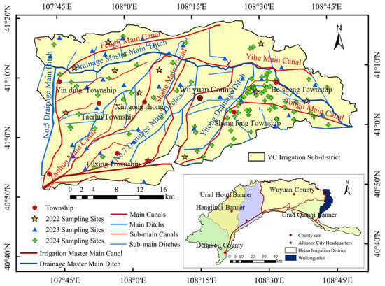
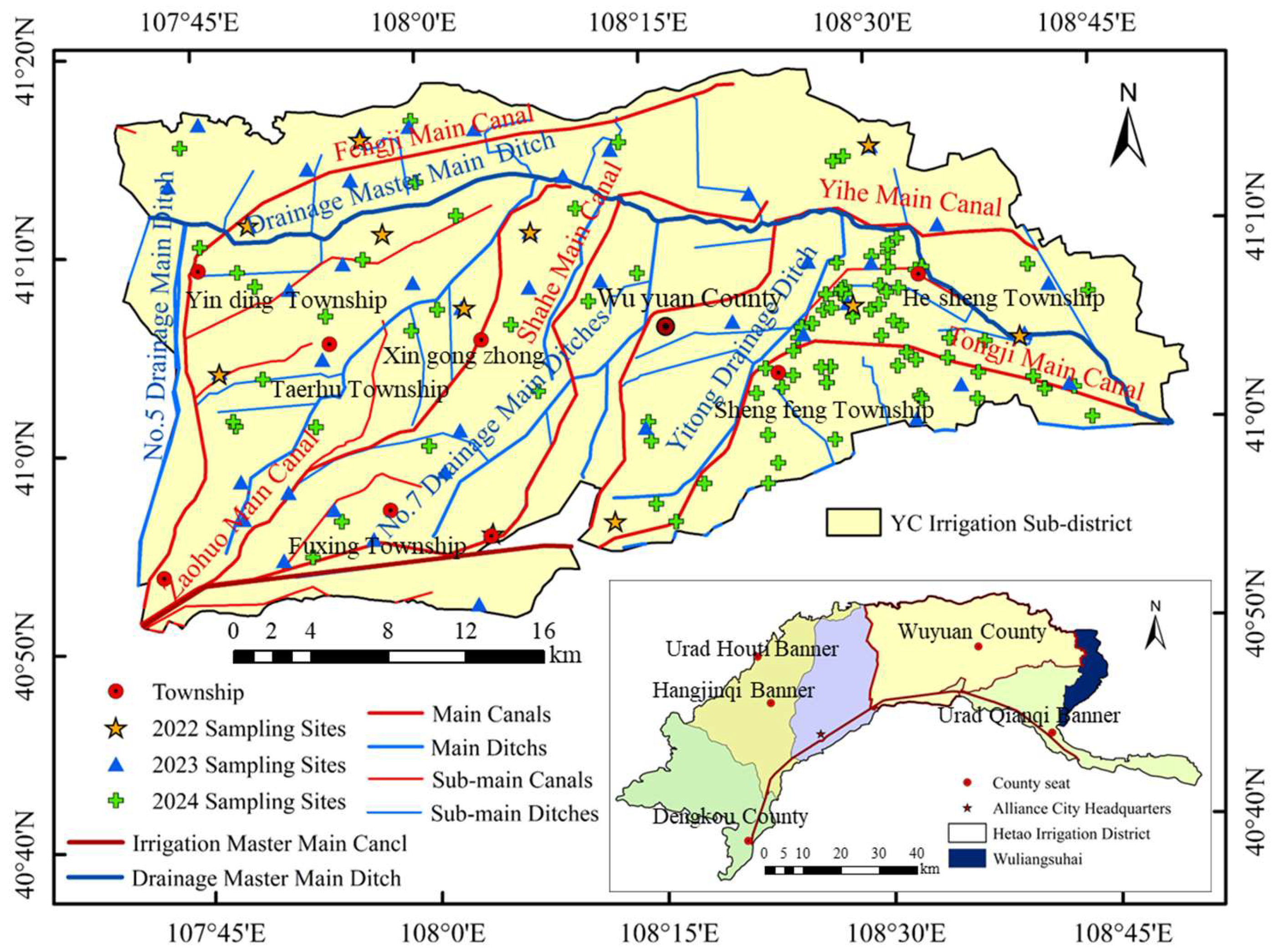
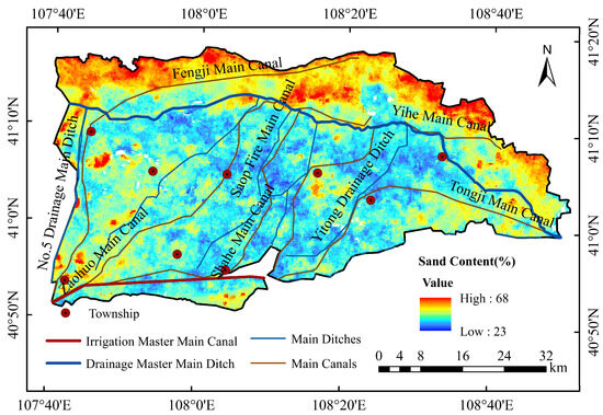
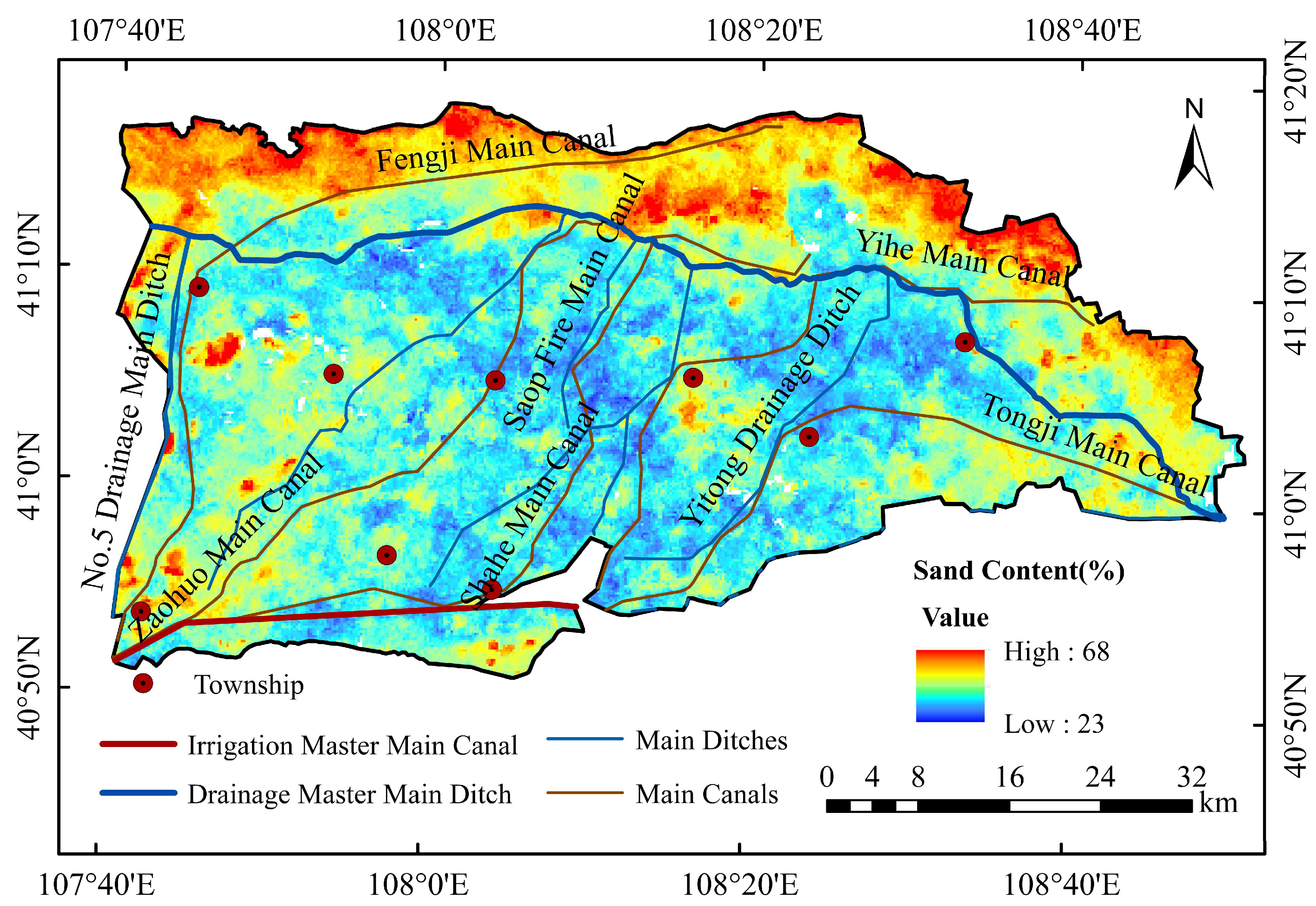
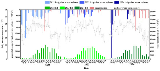
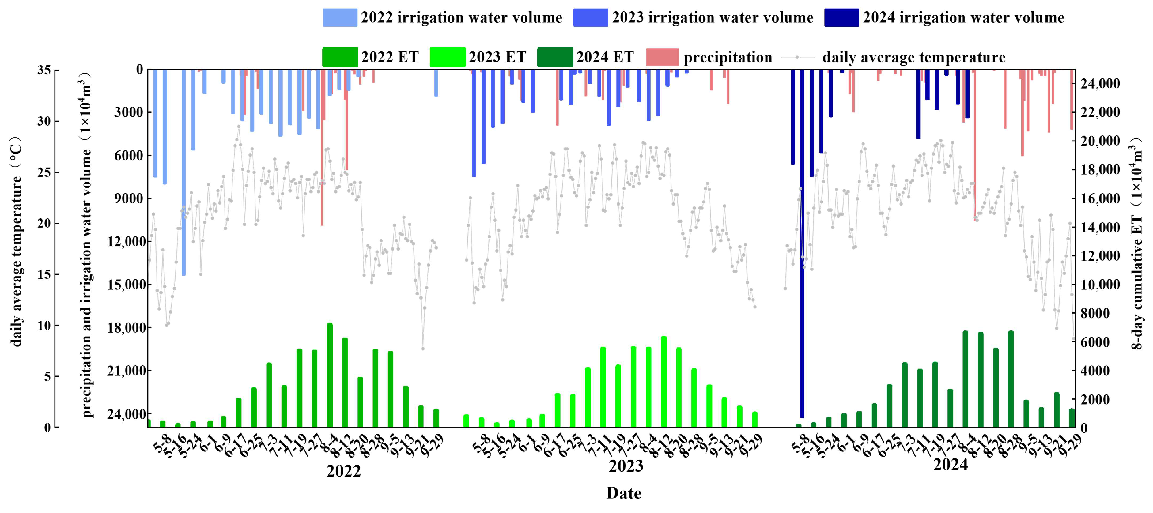
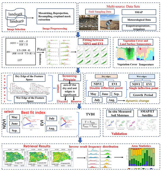
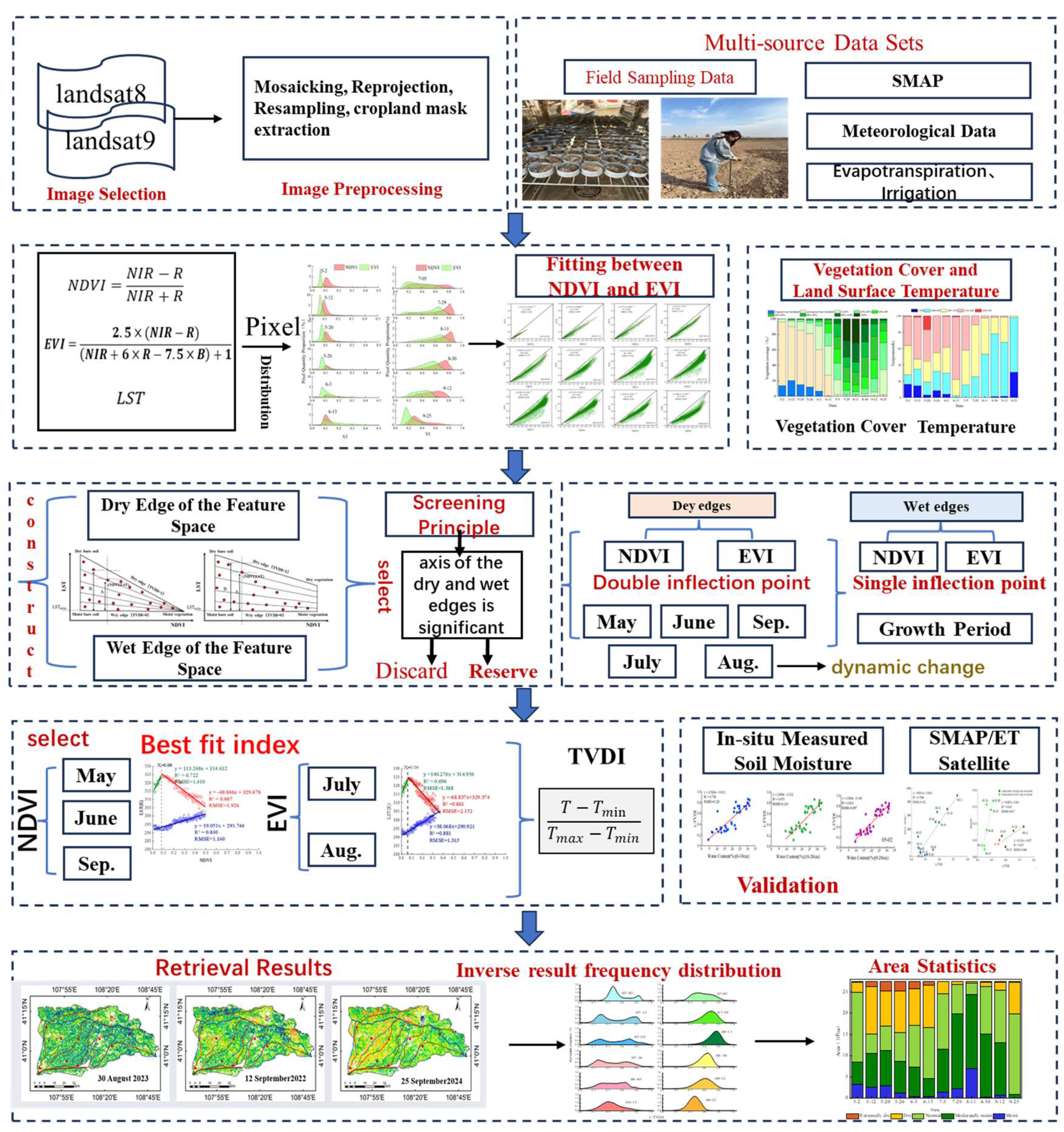
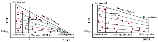
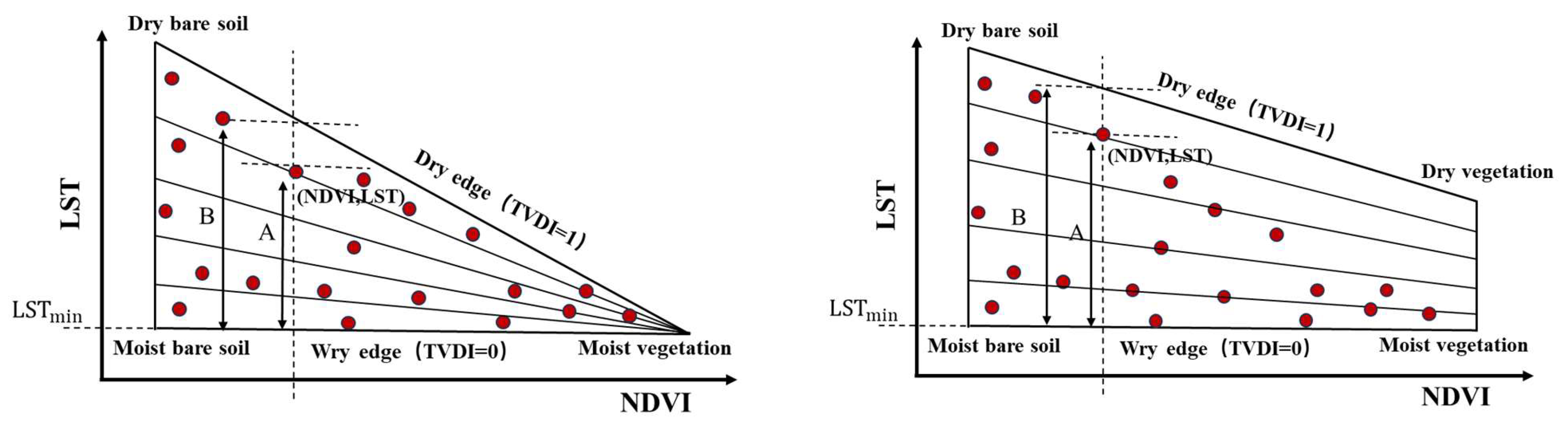
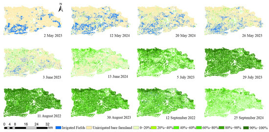
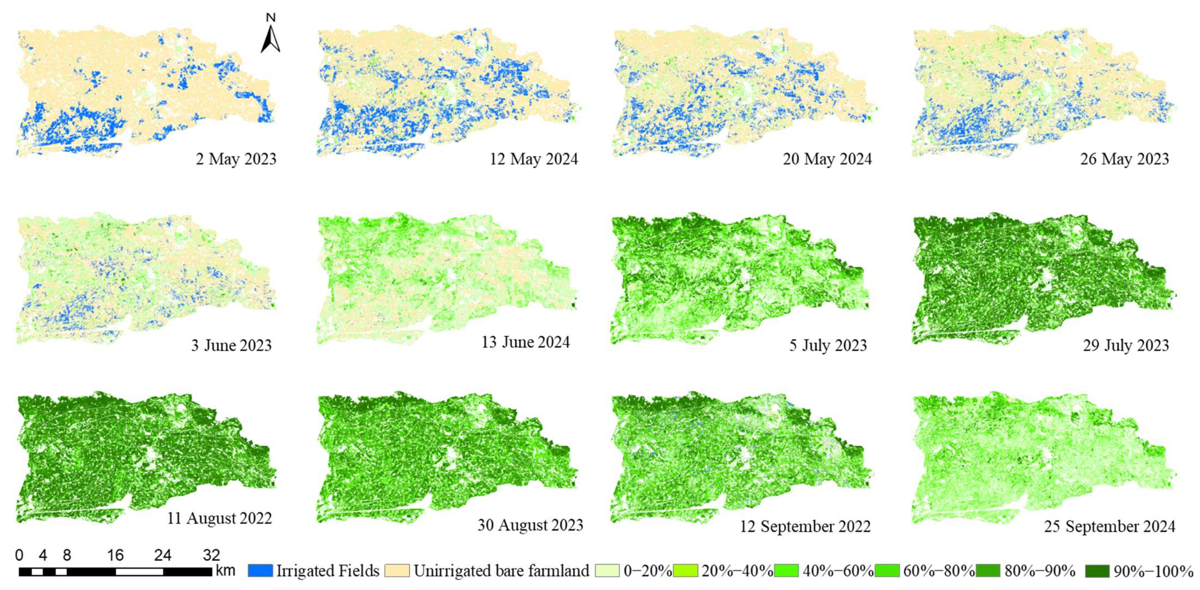
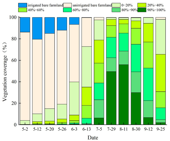
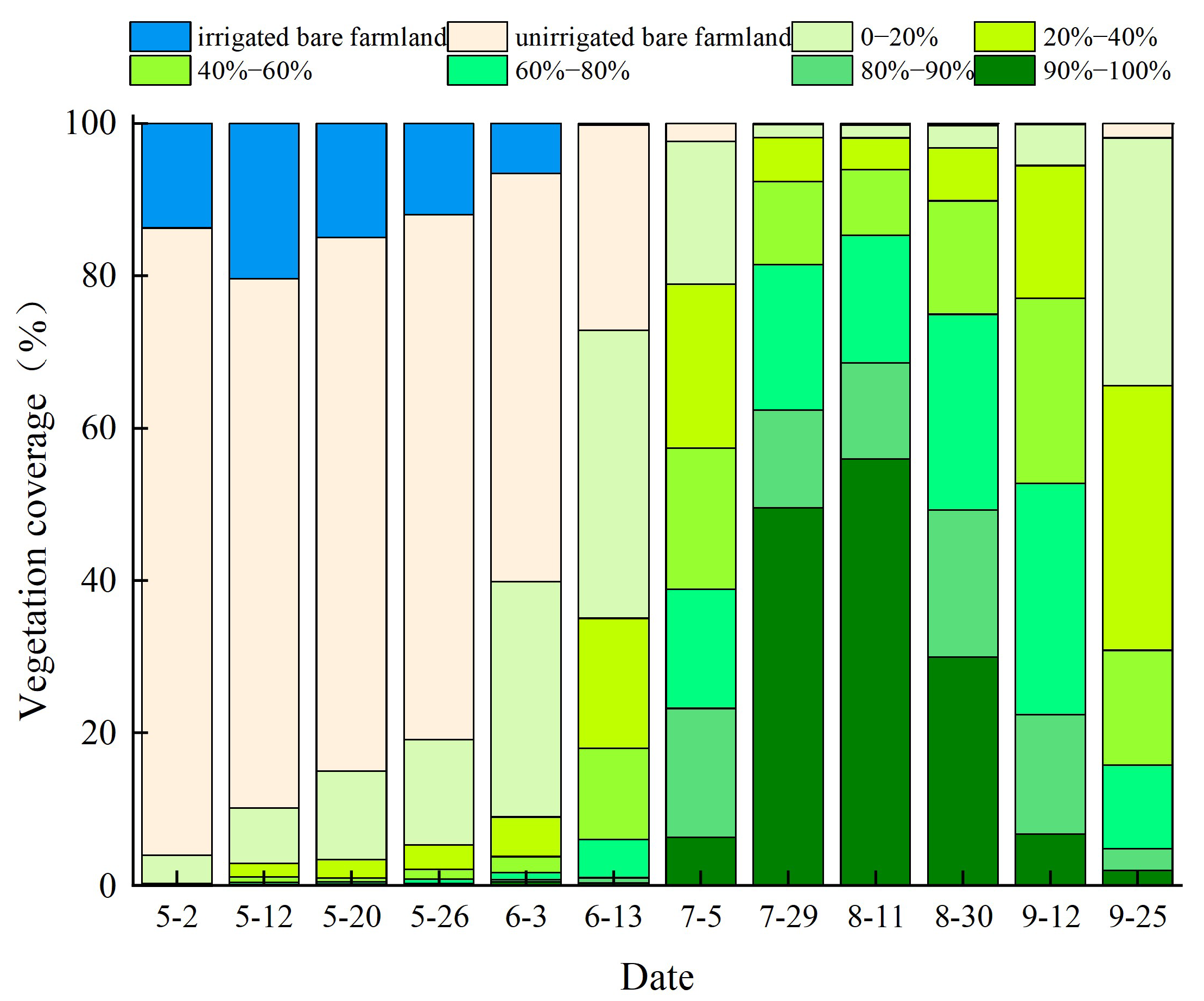
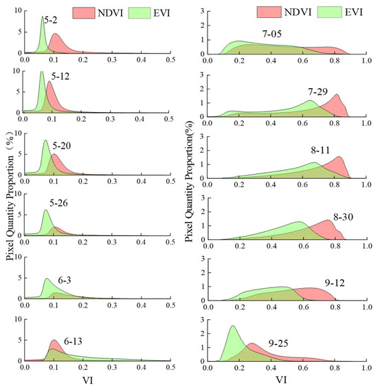
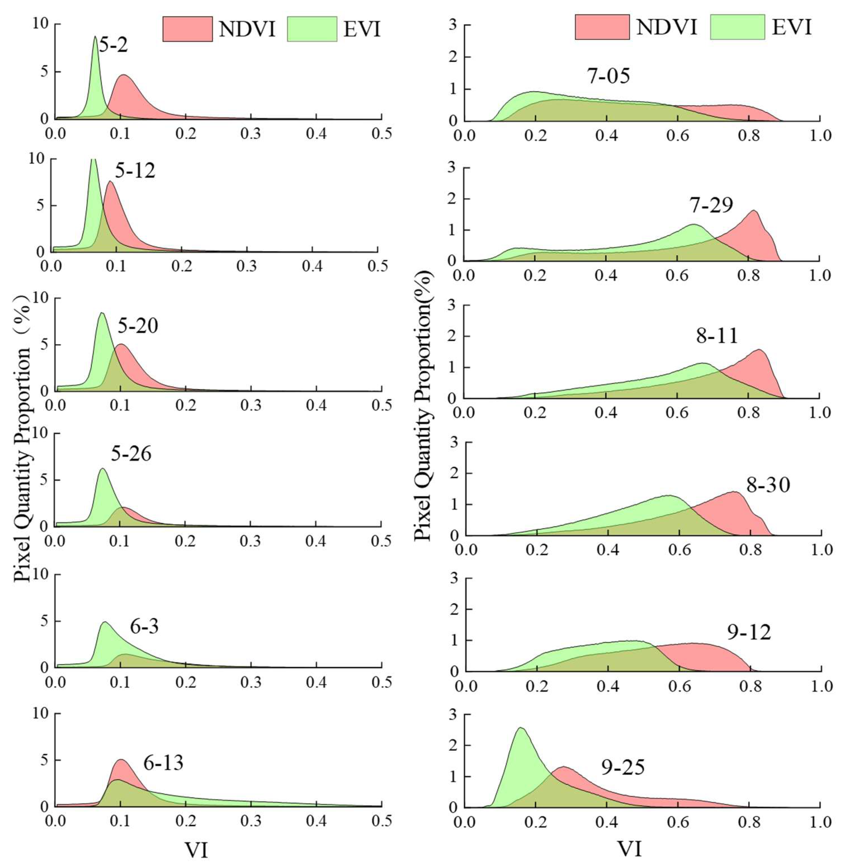
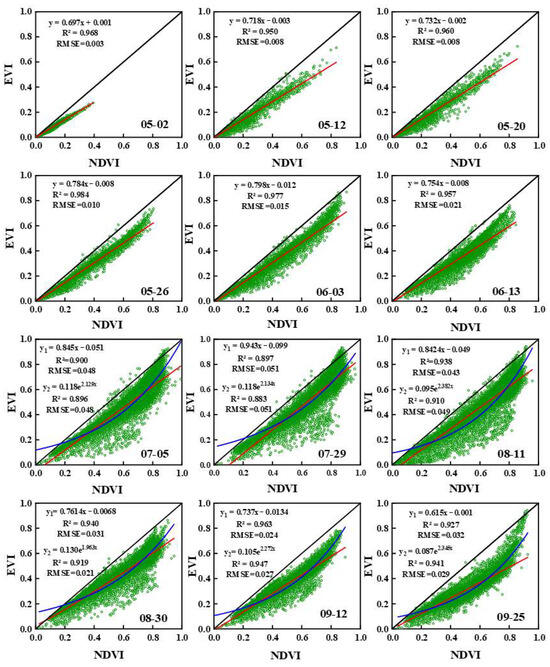
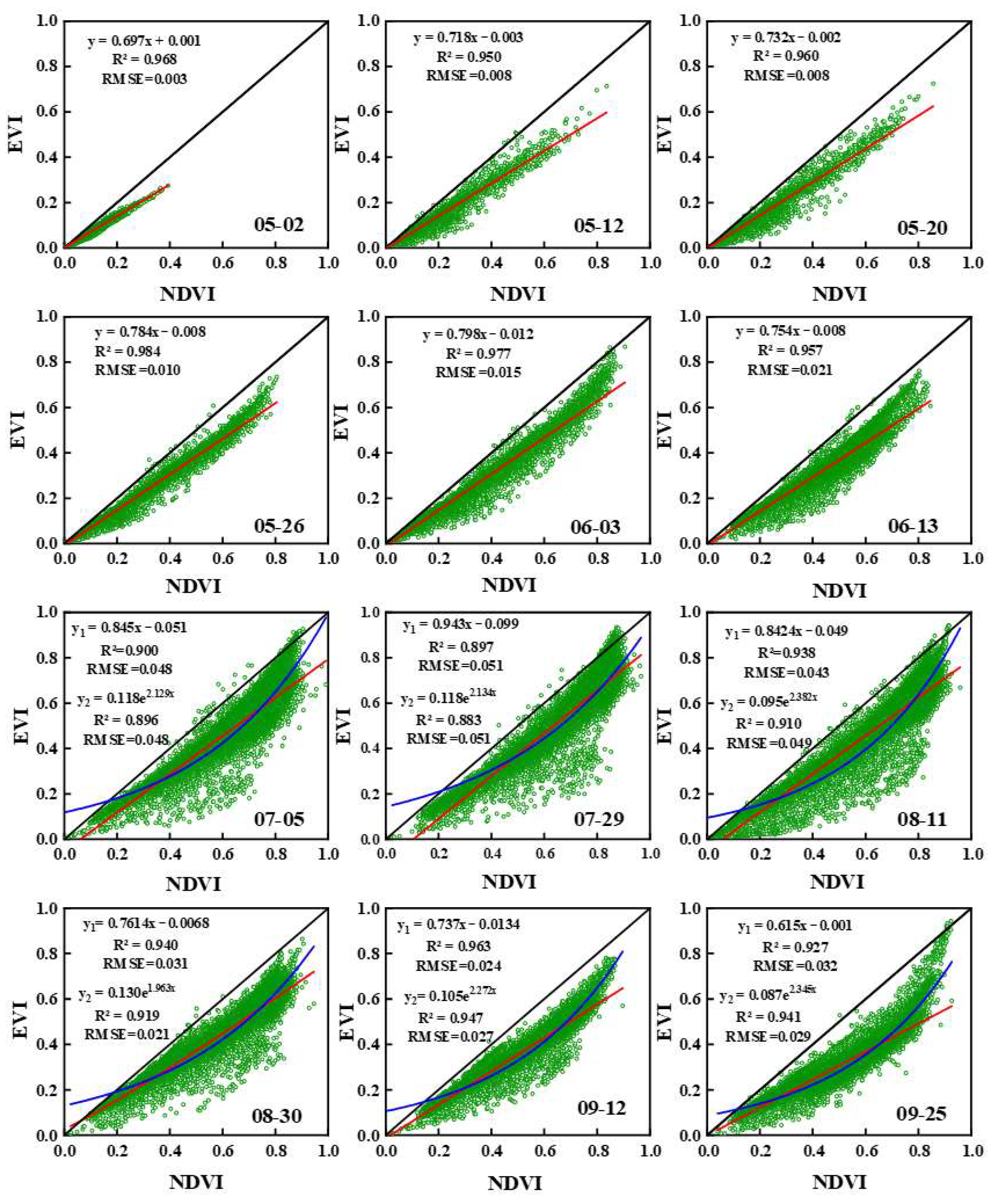
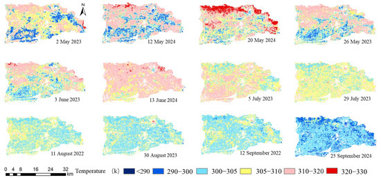
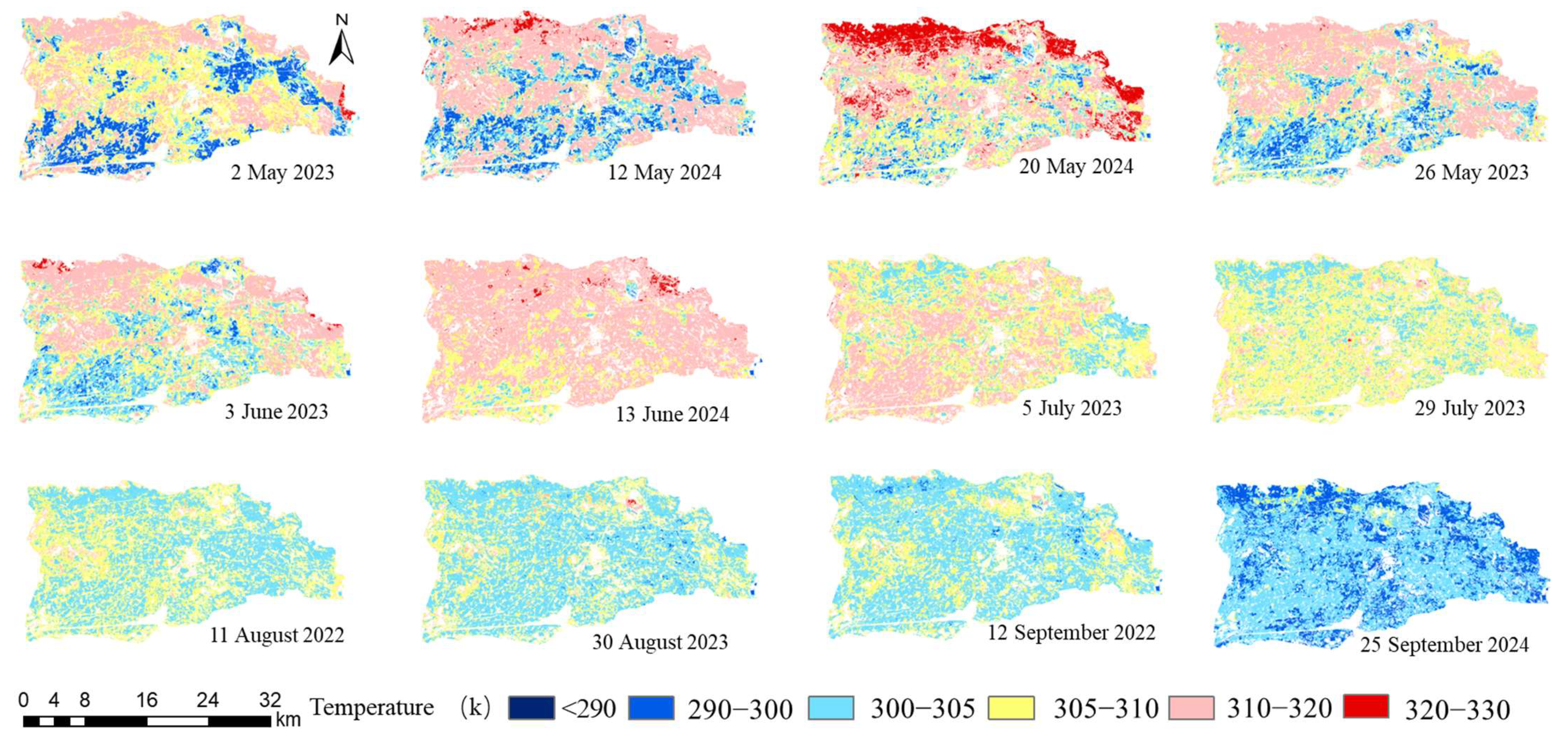
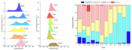
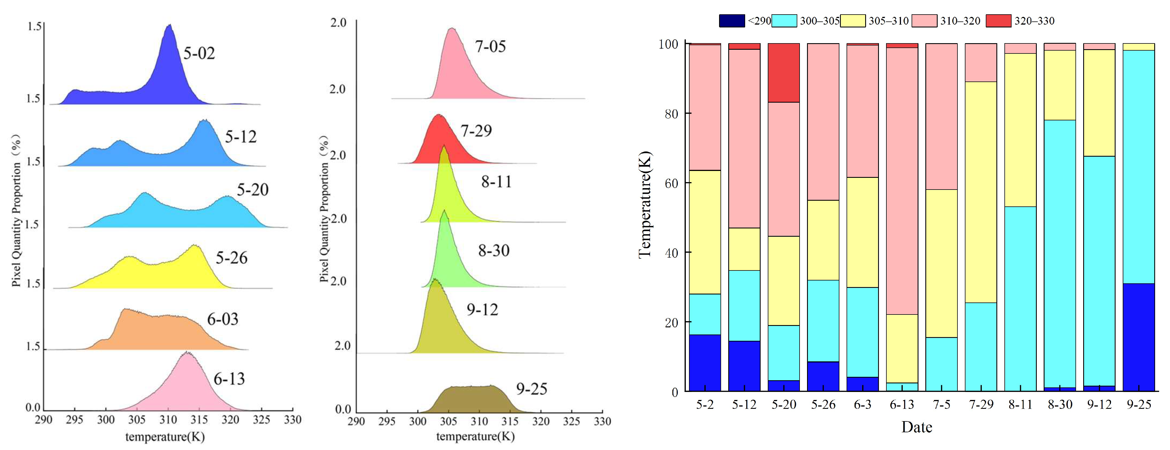
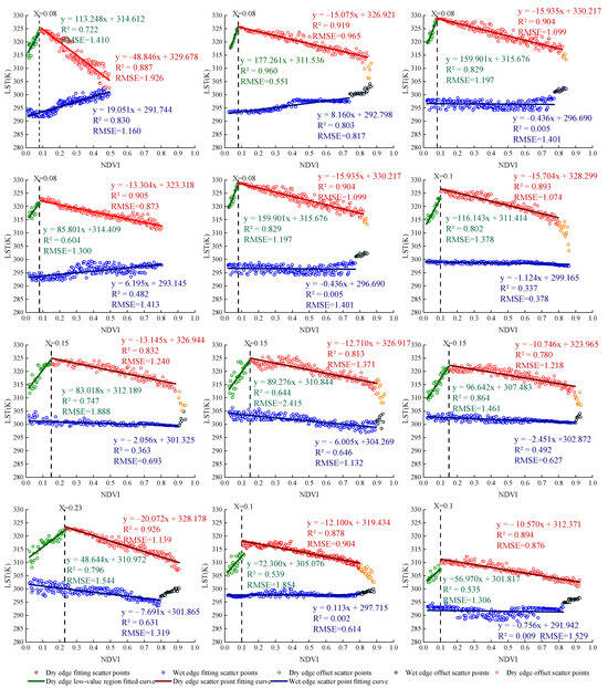
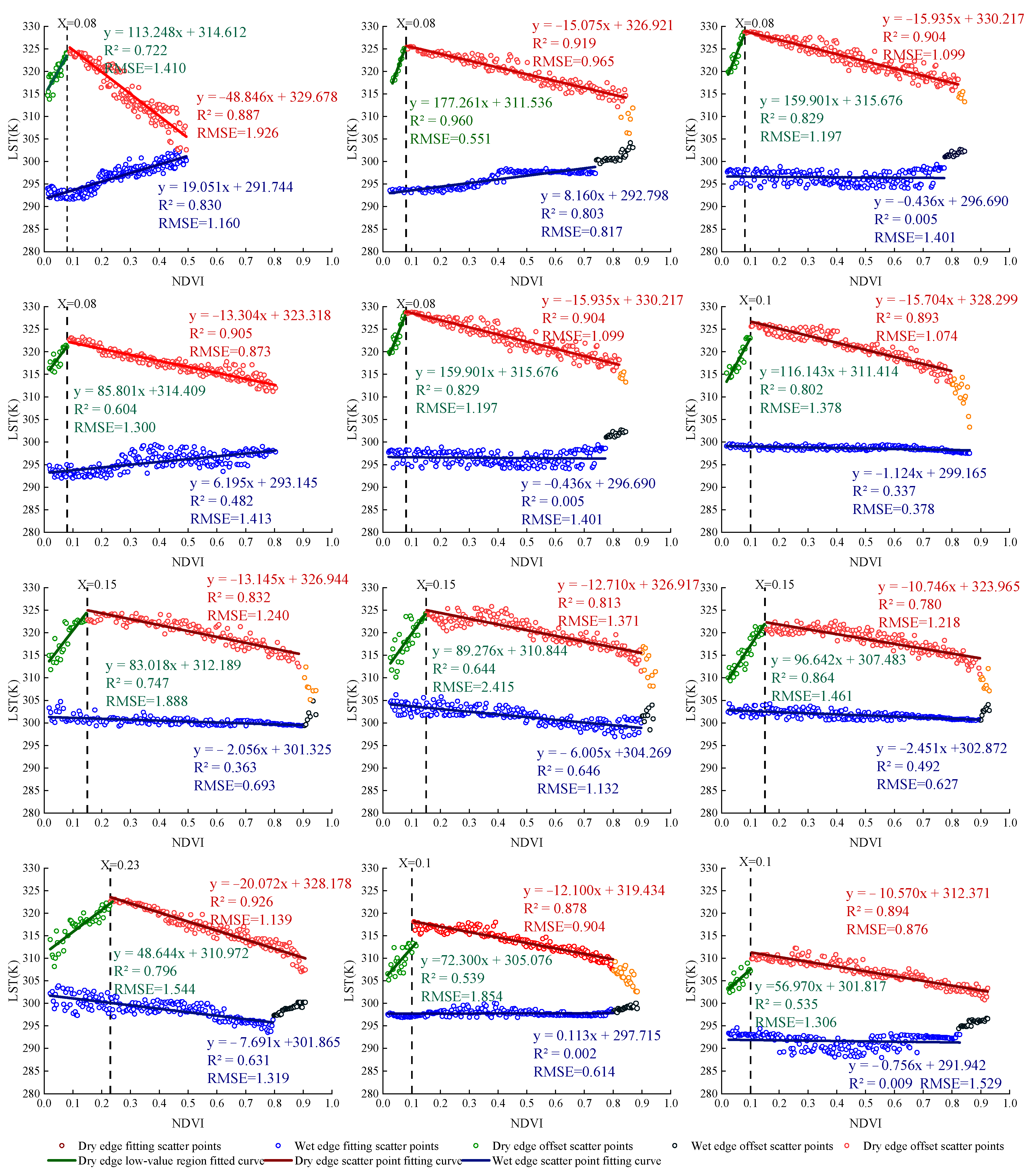
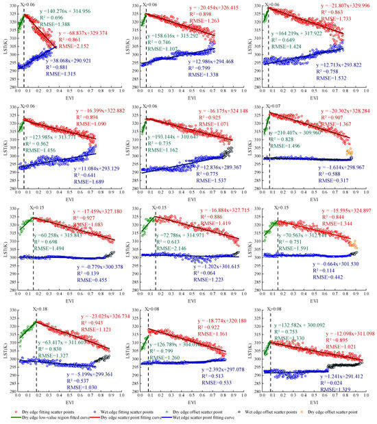
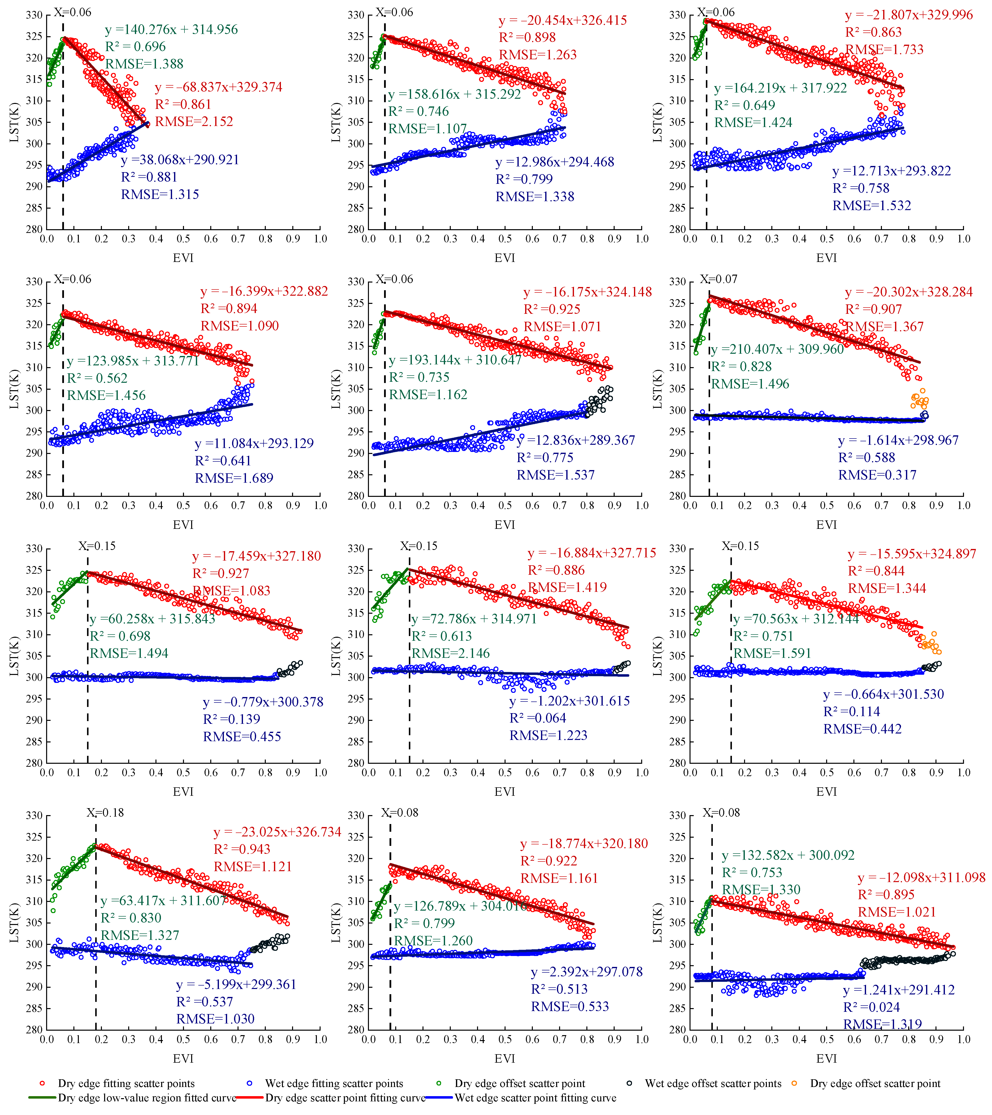
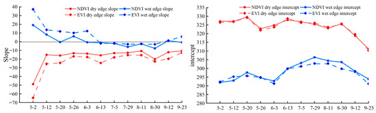
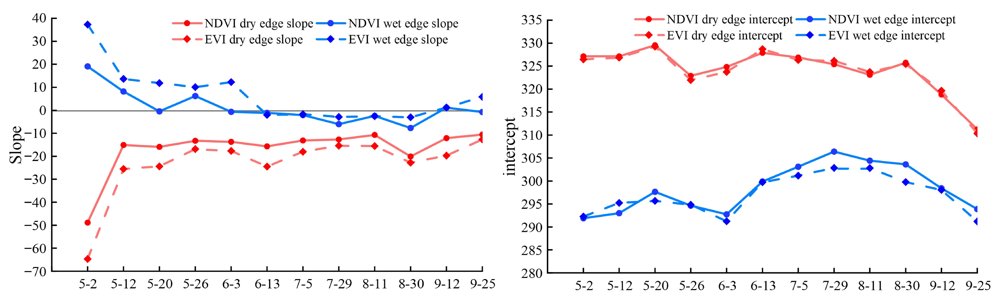
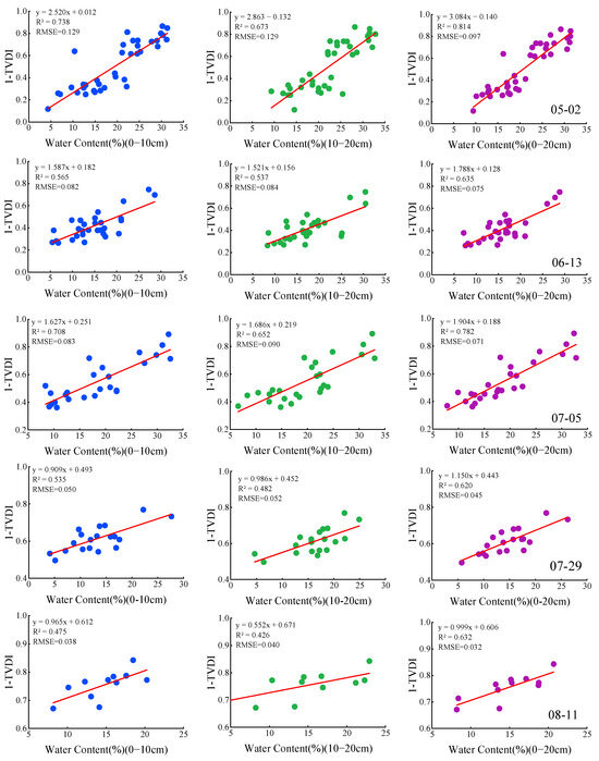
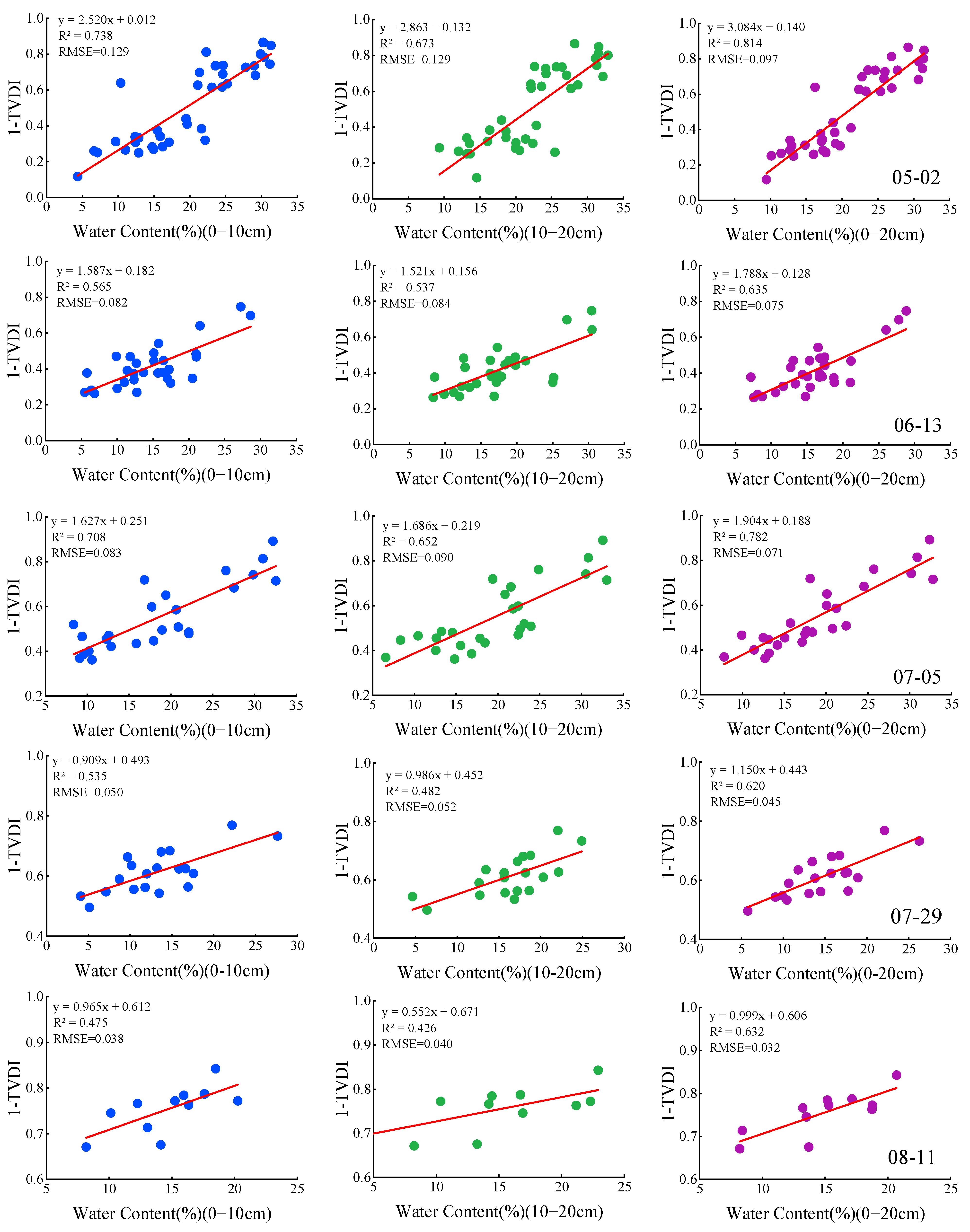
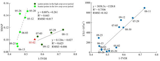
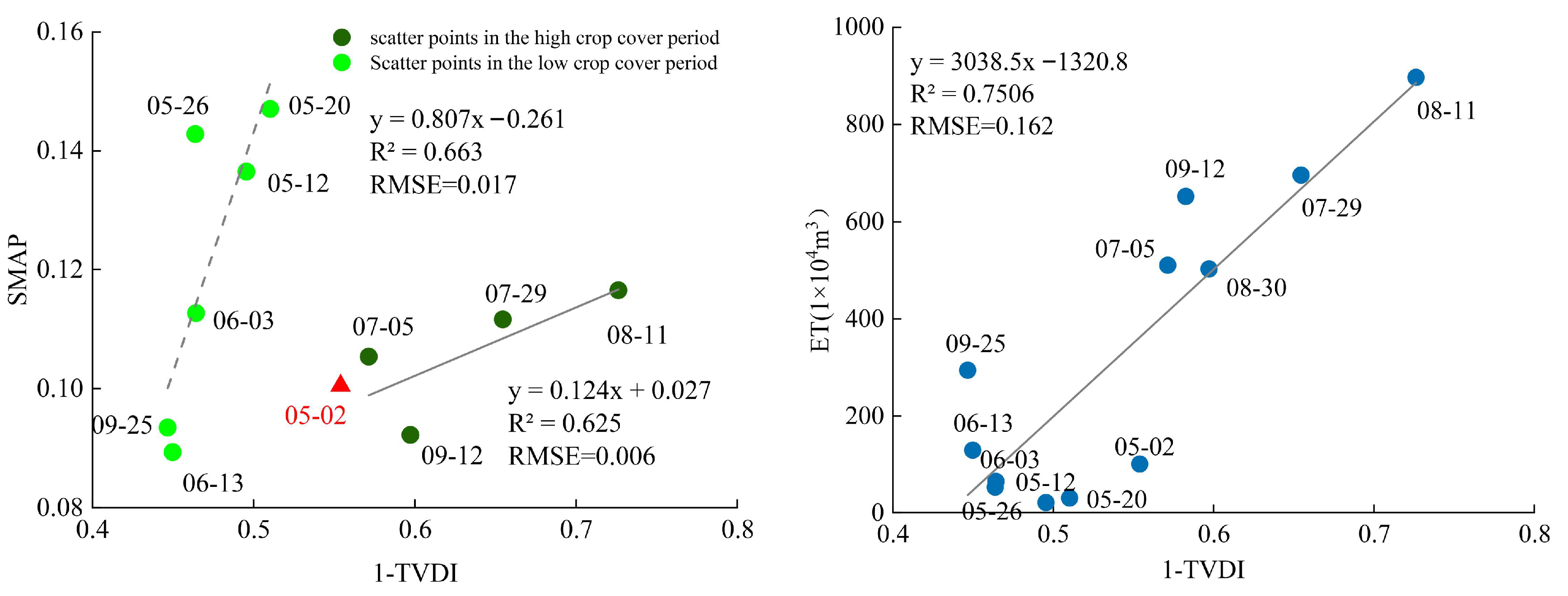
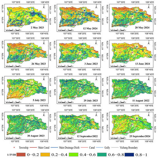
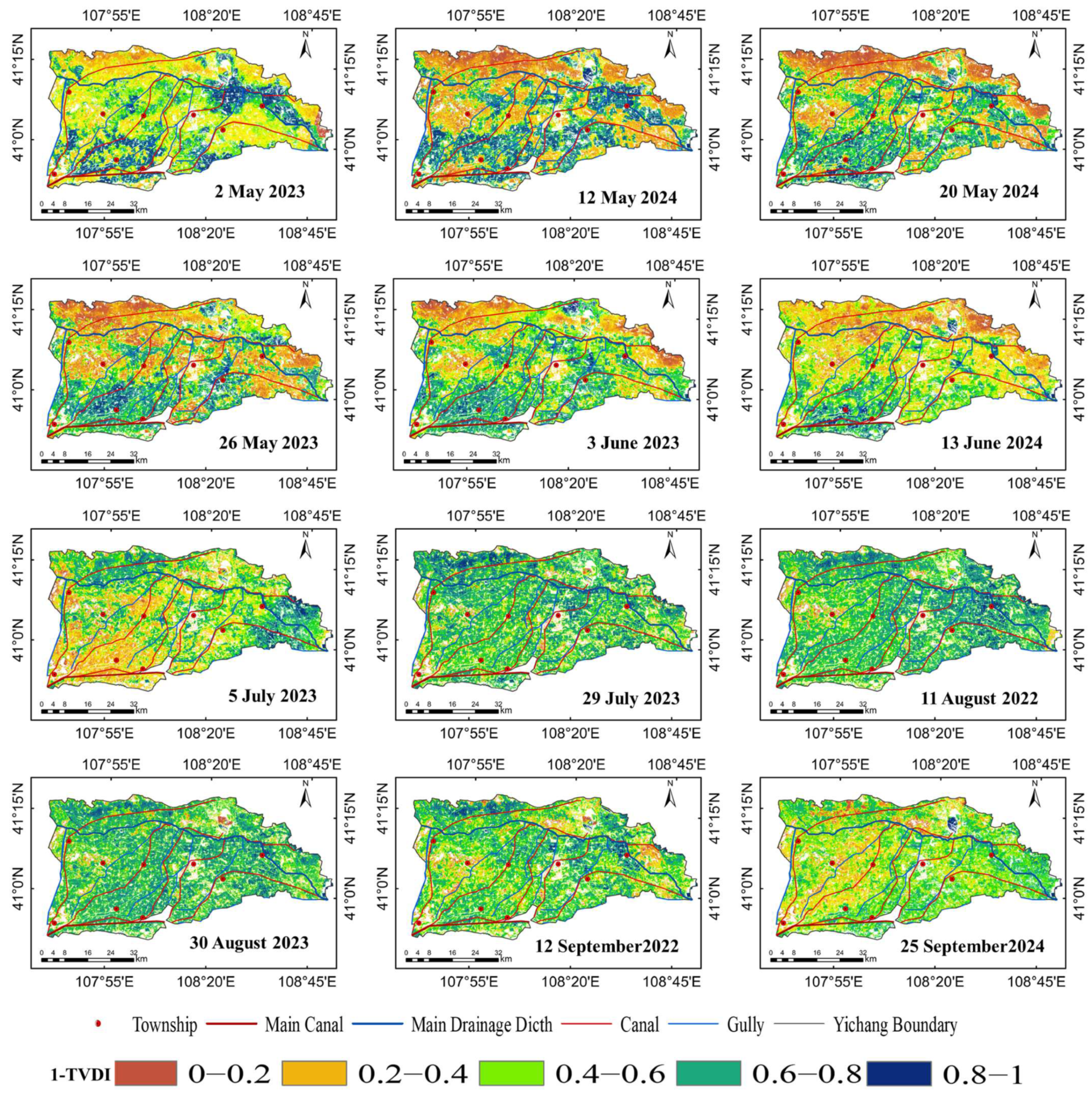
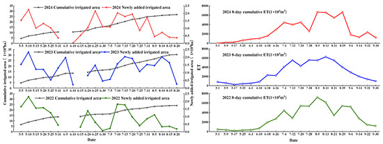
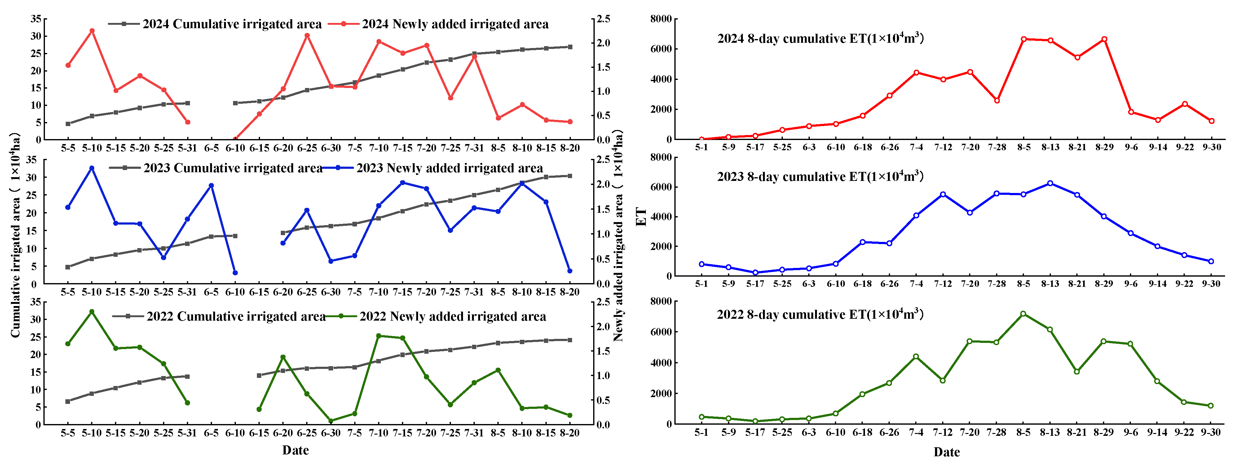
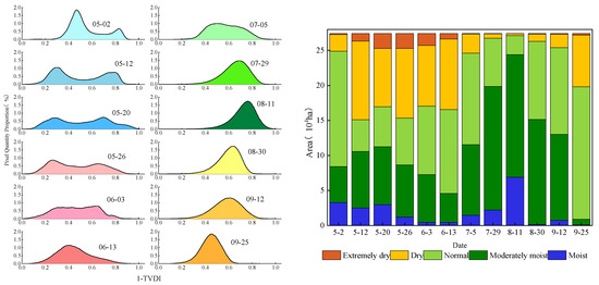
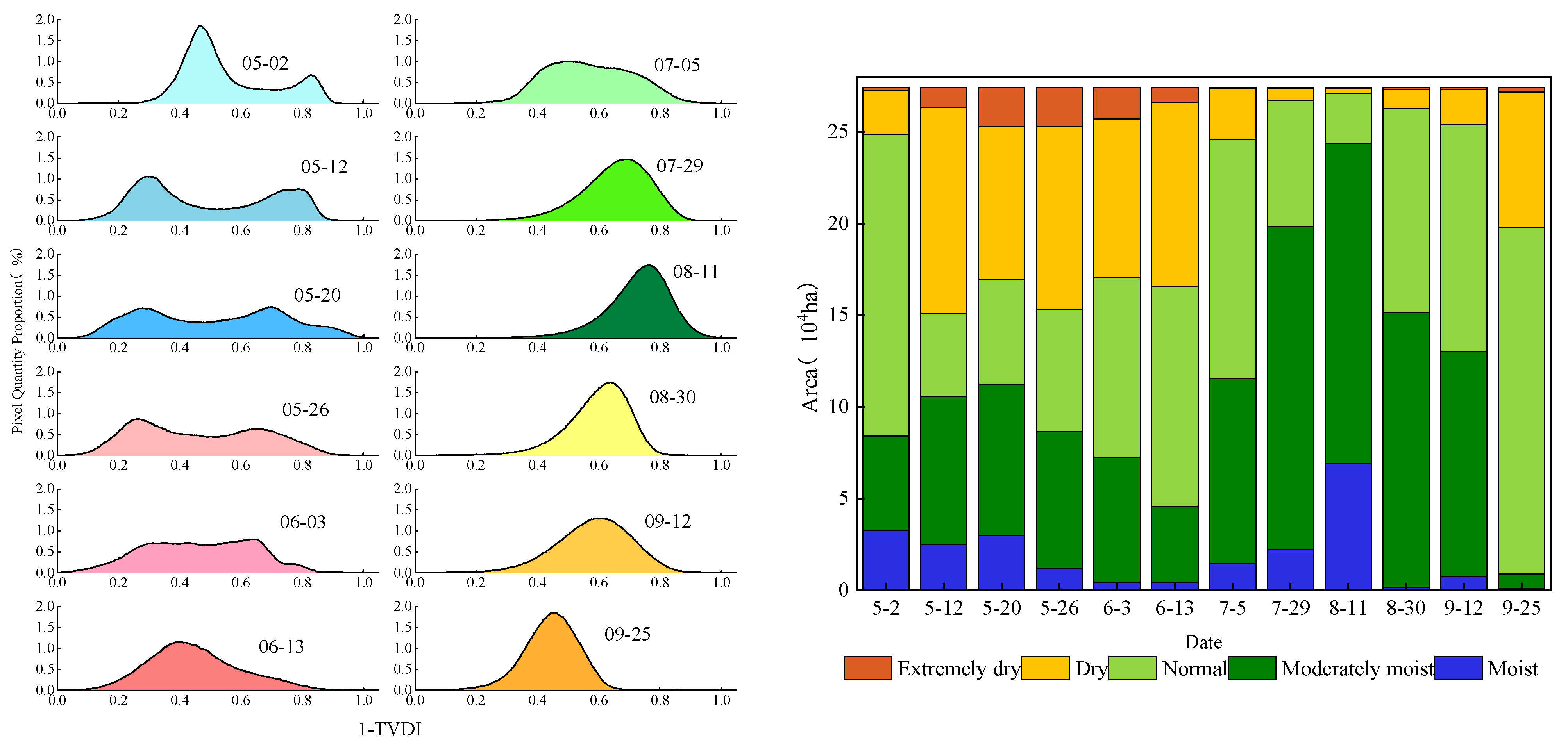

Disclaimer/Publisher’s Note: The statements, opinions and data contained in all publications are solely those of the individual author(s) and contributor(s) and not of MDPI and/or the editor(s). MDPI and/or the editor(s) disclaim responsibility for any injury to people or property resulting from any ideas, methods, instructions or products referred to in the content. |
© 2026 by the authors. Licensee MDPI, Basel, Switzerland. This article is an open access article distributed under the terms and conditions of the Creative Commons Attribution (CC BY) license.