


Abstract
We analyze annual yield and harvested area of domestic-consumption plantain (Musa AAB; export plantain excluded) in 31 continental Colombian departments from 2007 to 2025 (589 records). Bivariate yield and log-area trajectories are grouped with Partitioning Around Medoids (PAM) under Dynamic Time Warping (DTW) and synchronous Euclidean distance, and discrete-time Markov chains describe transitions among pooled yield quartiles. A three-group production-scale partition, which separates Arauca and Meta as the highest-yielding pair, is stable across 37 year-removal perturbations under both distances (10th-percentile adjusted Rand index = 1.000), but departmental means alone reproduce it and unequal weighting of yield and area changes it; the four-group DTW solution fails the stability criteria. Of 556 annual transitions, 75.54% remain in the same yield state, above a within-department permutation null (55.06%), yet transitions differ across departments, so the pooled first-order chain is descriptive. In rolling-origin comparisons for 2020–2025, adding climate reduces pooled root mean squared error (RMSE) by 37.6–45.9% in tree ensembles without lagged yield, but coordinates alone give larger reductions, and repeating the previous year’s yield gives the lowest RMSE (0.734 t ha−1). The results describe productive heterogeneity and persistence without establishing climatic or causal effects.
1. Introduction
Plantain (Musa AAB) contributes to food supply and rural livelihoods in Colombia, where agroindustrial research has examined sustainable innovation management within its production chain [1]. National analyses of fruit and vegetable statistics have also documented departmental differences in productivity and stability [2]. For plantain, simple multi-year averages do not show whether departments with similar mean yields arrived there through steady growth, contraction, or flat trajectories, nor how often a department shifts between yield levels from one year to the next.
Examining these records requires separating three aspects of longitudinal variation. First, when clustering bivariate trajectories of yield and harvested area, pooled standardization preserves departmental differences in level and dispersion, whereas within-department standardization removes these differences to emphasize normalized trajectory shape. Second, although DTW [3] allows short timing shifts between series, whether a two-year warping window produces more stable groups than synchronous Euclidean distance in a short annual panel must be tested directly against year removals. Third, whole-trajectory clusters are static over the study period; tracking year-to-year persistence and upward or downward movement requires a state-transition model such as a discrete-time Markov chain.
A further question is whether annual departmental climate improves yield prediction beyond productive history. Previous-year yield provides a simple baseline against which additional predictors can be evaluated. Comparing out-of-time predictions with and without climate variables from the National Aeronautics and Space Administration (NASA) Prediction Of Worldwide Energy Resources (POWER) project [4] and the Oceanic Niño Index (ONI) [5]—first using lagged area alone, and then using both lagged area and lagged yield—tests their incremental predictive contribution. Because the test-year climate is observed, this comparison is retrospective.
In this study, we analyze a multi-year plantain panel across 31 continental Colombian departments. The main contributions are as follows:
- We compare bivariate yield and log-area clustering under pooled standardization (production scale) and within-department standardization (trajectory shape) using PAM.
- We evaluate two-, three-, and four-group partitions under two-year DTW and synchronous Euclidean distance across all 37 single-year and adjacent two-year removals. The three-group production-scale typology is retained for profiling, four-group solutions are treated as a sensitivity analysis, and inter-departmental proximity is described through a minimum spanning tree (MST) and two-nearest-neighbor (2-NN) graph.
- We estimate annual transitions across pooled yield quartiles using discrete-time Markov chains, reporting retention, upward and downward mobility by cluster, a null model preserving departmental state frequencies, heterogeneity tests across clusters and departments, simulation-calibrated second-lag, duration, and subperiod homogeneity tests, and two-way panel-bootstrap intervals for long-run quantities.
- We test the out-of-time predictive contribution of ten agroclimatic and ENSO variables across five regression algorithms against a naive yield-persistence benchmark, complemented by held-out tree-based Shapley additive explanations (TreeSHAP) and three-year yield ratios around climatic anomalies.
Section 2 reviews related work on yield stratification, time-series clustering, Markov chains, and agroclimatic yield modeling. Section 3 describes the dataset, clustering and stability metrics, Markov estimators, and rolling-origin evaluation. Section 4 presents the empirical results and study limitations, and Section 5 summarizes the conclusions and future work.
2. Related Work
Previous work on agricultural yield series spans field-scale management zoning, national productivity panels, time-series clustering, Markov transition models, and climate–yield regressions. Here, we review the studies most closely related to our analysis of Colombian plantain records.
2.1. Productive Stratification and Yield Stability
At the field scale, multi-year yield maps are commonly grouped into zones that differ in mean productivity and inter-annual variability. Blasch et al. [6] combined principal component analysis (PCA), pixel-level stability metrics, and k-means clustering to summarize multi-year yield histories across four commercial fields in Australia and the United Kingdom. De Souza et al. [7] evaluated corn and soybean yield maps from three fields using the ratio of mean normalized yield to its temporal standard deviation, comparing partitions into two, three, and four zones. Earlier, Scudiero et al. [8] used local regression and fuzzy clustering on soil and crop sensor data across two maize seasons in Italy to show how zone boundaries shift over time. While these studies rely on high-density within-field monitors, regional and national panels aggregate heterogeneous farms into administrative units, where the analytical focus shifts from site-specific input prescription to territorial stratification.
In Colombia, Parra-Londono et al. [2] used national AGRONET statistics and linear mixed models to analyze yield stability across fruit and vegetable crops, and PCA to examine associations with non-climatic variables. For plantain (Musa AAB) specifically, recent domestic studies have examined agroindustrial chain management in Quindío [1] and soil-based nutrient models in Risaralda [9]. These studies provide context for comparing multi-year departmental yield–area profiles with annual yield-state transitions, which address different aspects of productive variation.
2.2. Elastic Distances in Time-Series Clustering
Clustering longitudinal trajectories requires choosing both a feature standardization and a dissimilarity measure. In large-scale benchmarks on the University of California, Riverside time-series archive, Javed et al. [10] compared Euclidean, DTW, and shape-based distances across eight clustering algorithms, and Holder et al. [11] extended the comparison to nine elastic distances under k-means and k-medoids. Javed et al. reported different distance rankings across clustering algorithms, while Holder et al. found that DTW generally did not outperform Euclidean distance in their experiments. These findings motivate an empirical comparison rather than an assumed advantage for temporal alignment.
Agricultural applications of elastic alignment include sub-seasonal remote sensing series; for example, Li et al. [12] paired a fast approximation to DTW (FastDTW) with hierarchical clustering on Sentinel-1 and Sentinel-2 time series to map winter crops in the United Kingdom. Unlike dense intra-seasonal reflectance curves, departmental agricultural statistics consist of short annual series (19 years in our panel) where both productive scale and normalized trajectory shape are of interest. These differences in temporal resolution motivate testing the contribution of alignment on annual statistical records rather than transferring its performance from remote sensing applications.
2.3. Markov Chains for Annual Yield Mobility
Whereas trajectory clustering assigns each territory to a single group over the full study period, discrete-time Markov chains model year-to-year movement across yield levels. Huzsvai et al. [13] applied finite-state Markov chains to Hungarian maize yields across two historical periods, defining failure, average, and high-yield states relative to a five-year moving Olympic average and estimating transition matrices and stationary distributions. Defining states relative to a local moving average captures short-term departures from a territory’s recent trend, whereas defining states from pooled sample quartiles tracks mobility across common national yield strata. The distinction matters when interpreting mobility: remaining in a national yield stratum differs from remaining close to a territory’s recent trend.
2.4. Agroclimatic Yield Modeling and TreeSHAP Attribution
Statistical and machine-learning models are widely used to quantify how temperature, rainfall, and large-scale ocean–atmosphere oscillations covary with crop yields. For Musa systems, Varma and Bebber [14] fitted empirical temperature and precipitation response surfaces to historical dessert-banana yields across 27 countries, documenting substantial regional variation in climatic sensitivity. For non-linear yield prediction, Huber et al. [15] compared Extreme Gradient Boosting (XGBoost) against deep neural networks for county-level soybean yields in the United States and used TreeSHAP [16] to summarize feature attributions. Such attributions describe a fitted model; assessing the additional predictive information in climate requires comparisons against an otherwise equivalent model without those variables.
3. Methodology
This section describes panel construction and the procedures used to characterize trajectories, estimate annual yield-state transitions, and evaluate complementary climate-related predictions and event-window ratios.
3.1. Overview of the Analytical Workflow
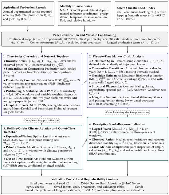
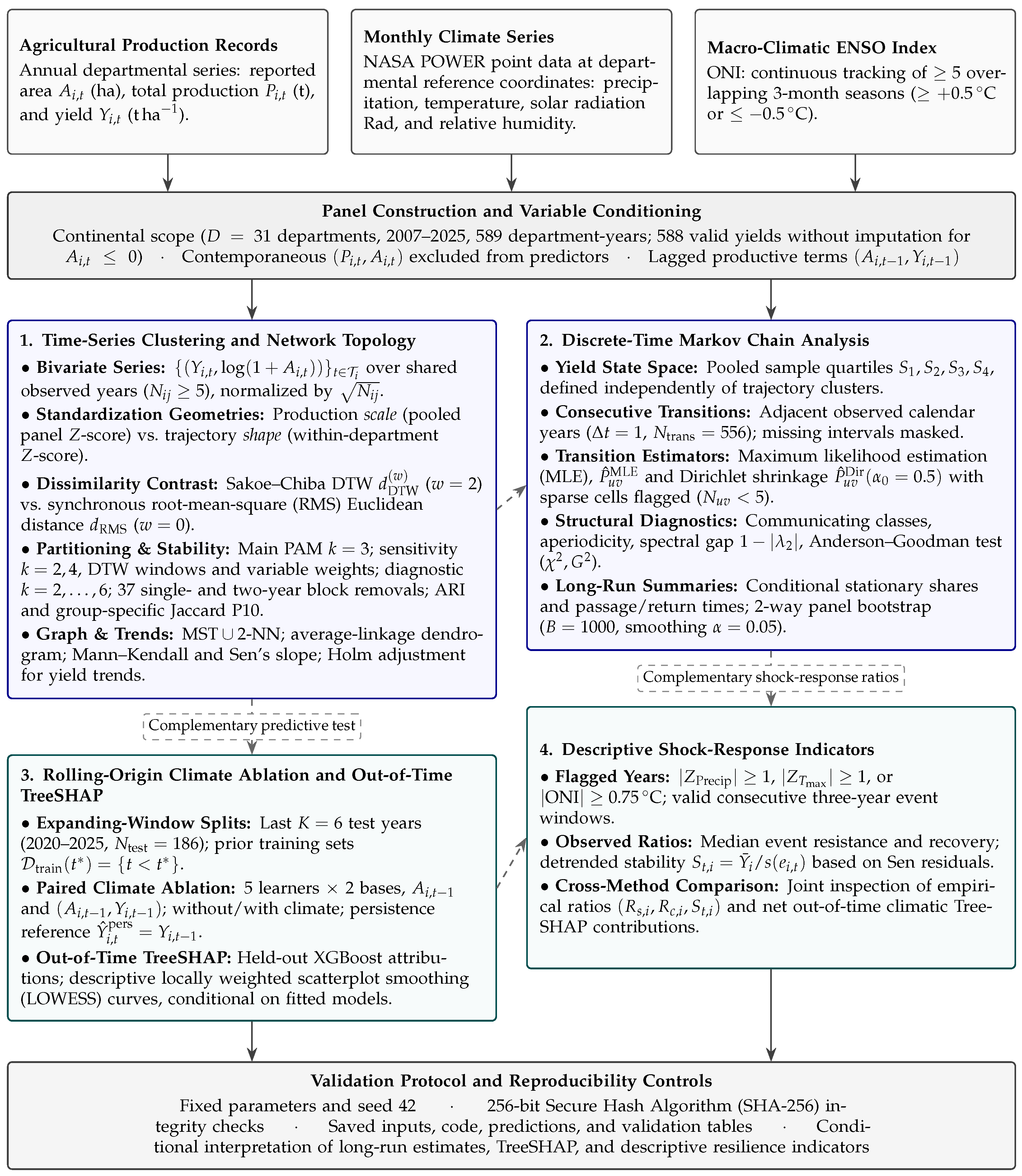
Figure 1 summarizes the four analytical stages following data preparation. Time-series clustering and Markov chains constitute the core longitudinal analysis, whereas rolling-origin predictive comparisons, TreeSHAP attributions, and shock-response ratios provide complementary evaluations. Departmental clusters summarize full multi-year trajectories of yield and harvested area, whereas Markov states classify individual annual yields; cluster assignments are used only to stratify transition summaries.
Figure 1.
Analytical workflow. Solid arrows indicate data flow; dashed links indicate descriptive comparisons across components. The primary analysis separates multi-year departmental trajectory clusters from annual yield states, while rolling-origin climate comparisons and shock-response ratios are evaluated independently.
3.2. Study Scope, Panel Construction, and Agroclimatic Data
The Colombian agricultural dataset was obtained from Agronet’s departmental statistics. The underlying Evaluaciones Agropecuarias Municipales are published as two open municipal datasets: the historical base of the Ministerio de Agricultura y Desarrollo Rural for 2006–2018 [17] and the base of the Unidad de Planificación Rural Agropecuaria (UPRA) for 2019–2025 [18]; the portal’s source notes label these periods 2016–2018 and 2019–2025 [19]. The panel corresponds to Agronet’s plantain subcategory for domestic consumption, which excludes export plantain (reported in Antioquia, Caldas, Cauca, Chocó, La Guajira, and Risaralda) and the cachaco type. The dataset comprises annual departmental records of harvested area (, ha), production (, t), and yield (, t ha−1) for plantain in Colombia from 2007 to 2025. The source labels yield as ha/ton, but its values match production divided by area in t/ha within an absolute tolerance of ; only the header is corrected, without transforming the reported values. The analysis covers the 31 continental departments, excluding the 14 insular records for San Andrés y Providencia (2012–2025) retained in the original dataset, resulting in 589 department–year observations over 19 calendar years.
Records are screened for missing identifiers, duplicate department–year keys, and out-of-range values without imputing missing years or yields. Because Amazonas reports zero harvested area in 2009, its yield for that year is undefined, leaving 588 valid yield observations. Regression baselines use only one-year lagged area () and, in dynamic specifications, one-year lagged yield (), restricted to consecutive observed calendar years; contemporaneous area and production are excluded from all predictive models.
Monthly agroclimatic series are retrieved through the NASA POWER monthly point application programming interface (API) [4] at one reference point per department: the municipal seat of the municipality with the largest cumulative production of domestic-consumption plantain in the municipal records for 2007–2025 [17,18] (Appendix A). Monthly mean daily precipitation rates (mm day−1) are multiplied by month length and summed to annual precipitation (), while the intra-annual precipitation coefficient of variation (CV; ) and the count of dry months (<100 mm) are computed from the 12 monthly totals. Annual relative humidity (, %) and solar radiation (, MJ m−2 day−1) are calculated as arithmetic means of complete 12-month profiles. Annual maximum temperature (, °C) is the arithmetic mean of the 12 monthly POWER T2M_MAX values. Each monthly value is the highest daily maximum of that month rather than the mean of its daily maxima, so summarizes monthly temperature peaks and is higher than the annual mean of daily maxima. To assess how representative these single points are, annual precipitation is compared with CHIRPS v2.0 [20] at the same coordinates (Appendix A, Table A1).
Macro-climatic variability is tracked through ONI, supplied by the National Oceanic and Atmospheric Administration (NOAA) Climate Prediction Center (CPC). Following the historical CPC episode criterion [5], warm (El Niño) and cold (La Niña) episodes are identified on the continuous sequence of overlapping three-month seasons when ONI ≥ +0.5 °C or ONI ≤ −0.5 °C for at least five consecutive seasons, preserving episodes that cross calendar-year boundaries. For this study, each calendar year is assigned the majority qualifying regime (or neutral/transition when tied or below threshold), alongside the annual mean and its one-year lag . The annual classification is a study-specific aggregation of the seasonal episodes.
3.3. Time-Series Dissimilarity, Scale-vs.-Shape Clustering, and Network Topology
Each department is represented by its bivariate trajectory of yield and log-transformed area . To separate productive magnitude from temporal profile, two standardizations are evaluated. The production-scale representation standardizes each variable using the pooled mean and population standard deviation :
The trajectory-shape representation standardizes each series using its within-department mean and standard deviation (mapping constant series to zero):
For any department pair , let denote the shared calendar years with complete bivariate observations (), and let . An admissible warping path starts at , ends at , and advances by steps in . Building on the Sakoe–Chiba band constraint [3], our implementation restricts both index and calendar-year displacement: and . The DTW distance normalized by shared support is
Published benchmarks motivate comparing elastic and Euclidean distances rather than presuming an advantage for DTW [10,11]. Sensitivity to these fixed choices is assessed by repeating the PAM evaluation with windows under equal weights, and with weights of 0, 0.25, 0.75, and 1 for standardized yield (the remainder for log-area) under ; weights multiply the squared differences of each variable in the DTW cost. Here, we set years and compare against the synchronous RMS Euclidean distance on the exact same shared observations. Because the diagonal path is admissible for , holds algebraically; empirical clustering performance is therefore evaluated through perturbation stability rather than distance magnitude.
Candidate partitions are evaluated across using PAM [21], the unweighted pair group method with arithmetic mean (UPGMA; average linkage), and complete linkage. Our PAM implementation uses 15 random starts and up to 100 swap iterations; it does not implement the accelerated variants proposed by Schubert and Rousseeuw [22]. The three-group PAM partition under production scale (, ordered by ascending mean yield), which satisfies the operational criteria below under both distances, is retained for territorial profiling. PAM solutions for are compared across both geometries and distances, with reported as a sensitivity analysis. As a reference without temporal information, PAM is also applied to the standardized departmental means of yield and log-area under the same year removals.
Temporal sensitivity is quantified across all deterministic perturbations obtained by removing each single calendar year and each pair of adjacent calendar years, refitting the standardization, distance matrix, and clustering from scratch. Stability is summarized by the P10 of the ARI [23] () against the full-panel partition and by the worst-group P10 Jaccard [24] match:
Common-year ARI compares the full-panel partition with a partition refitted using only years with complete bivariate observations for all departments (18 years, excluding 2009). Operational reference thresholds are set at silhouette width [25] , , , and common-year (with at least 90% valid perturbations). These thresholds are study-specific diagnostic rules rather than statistical confirmation of distinct territorial regimes.
To visualize inter-departmental proximity, an undirected graph is formed by uniting the MST of with its symmetric 2-NN links. Edge lengths equal for MST construction, closeness, and shortest-path betweenness centrality, whereas eigenvector centrality uses Gaussian radial weights:
where is the median positive pairwise distance. Departmental yield and area trends are estimated via ordinary Mann–Kendall tests [26,27] and Theil–Sen slopes [28,29], applying Holm sequential step-down adjustment [30] across the 31 departmental yield tests. Group differences are described by medians and ranges of departmental means, with effect sizes from Kruskal–Wallis [31] and from one-way analysis of variance (ANOVA). Because yield and area define the clusters, no p values are reported for them; Kruskal–Wallis and ANOVA p values for the five climate variables are exploratory and Holm-adjusted across the five.
3.4. Discrete-Time Markov Chains and Ergodicity Diagnostics
The 588 valid annual yields are discretized into four pooled quartile states with fixed boundaries over the study period: (<), (), (), and (≥). Restricting transitions to consecutive observed calendar years within the same department yields 556 valid pairs .
Let denote the transition count from state u to v and . Transition probabilities are estimated via MLE and symmetric Dirichlet smoothing:
using as a sensitivity check and flagging cells with as sparse. Retention (), upward mobility (), and downward mobility () are computed on the pooled panel and stratified by DTW cluster.
Irreducibility and aperiodicity are verified via strong connectivity and self-loop structure of the positive-probability transition graph, alongside the spectral gap . Temporal homogeneity between the early () and late () subperiods is evaluated using the Anderson–Goodman Pearson () and likelihood-ratio () statistics [32]:
where , summing over rows supported in both subperiods and cells with positive pooled probability, with degrees of freedom .
When the chain is ergodic, the stationary distribution satisfies with , and mean first passage times to (with mean return times on the diagonal) are derived from the fundamental matrix. Uncertainty is summarized via 1000 two-way pigeonhole panel bootstrap replicates that independently resample departments and calendar years [33], applying minor Dirichlet regularization () within each replicate to ensure well-defined passage-time inversions.
Transitions enter the bootstrap as pre-formed pairs observed in consecutive calendar years, indexed by department and destination year. Each replicate multiplies the resampled weight of the department by that of the destination year and applies it to the whole pair, so zero weights only remove observed pairs and no artificial year pair can be created. A replicate is therefore a weighted set of pairs rather than a reconstructed series: this suffices for first-order transition counts, but independent year draws do not preserve order across more than two years or the dependence between adjacent pairs that share a year. Sensitivity is evaluated by resampling departments only, years only, and departments together with moving blocks of 2, 3, or 5 contiguous destination years, and by re-estimating the quartile boundaries within each replicate from the yields of the resampled pairs.
To separate persistence from stable departmental yield levels, observed retention is compared with a null model that randomly permutes the years within each department (10,000 permutations). This preserves each department’s state frequencies while removing temporal order; one-sided p values are computed as the proportion of permutations, including the observed arrangement, with retention at least as high as observed. Heterogeneity of transitions among clusters and among departments is evaluated with a likelihood-ratio statistic conditional on the origin state,
where g indexes the groups. Because many cells are sparse, p values are obtained from 10,000 permutations of group labels among transitions sharing the same origin state. Cluster contrasts are descriptive because clusters are defined from the same yield series.
Irreducibility, aperiodicity, and non-rejection of temporal homogeneity do not establish that one lag is sufficient or that departments share a transition mechanism, so three further diagnostics are reported. A second-lag statistic tests, within each state at , whether the state at t depends on the state at . A duration statistic tests, within each origin state, whether leaving that state depends on the years already spent in it (1, 2, 3, or ≥4), excluding spells left-censored at the start of a series. Temporal homogeneity is also evaluated for vs. , the boundary between the two source labels in the portal. Because counts are sparse, the p values of these likelihood-ratio statistics are calibrated with 10,000 simulations from first-order chains that preserve each department’s initial state and observed years. Null A uses the pooled matrix. Null B uses department-specific matrices shrunk toward it, , with and as study-specific settings. Rejection under A but not under B is compatible with differences between departments rather than additional memory within departments.
3.5. Rolling-Origin Climate Comparisons and Out-of-Time TreeSHAP
Out-of-time predictive evaluation uses expanding rolling-origin splits over the six test years [34]:
All paired models share the exact same complete-case cohort ( department–years). Departmental climate anomalies ( and ) and feature scalers are fitted strictly within at each split. Test-year climate is observed contemporaneously, so this protocol evaluates retrospective prediction for departments represented in training; it does not evaluate ex ante forecasting or transfer to unseen departments.
Five regression models are evaluated under fixed hyperparameters: Random Forest [35] (500 trees, depth 10), XGBoost [36] (350 trees, depth 4, learning rate 0.04), Light Gradient Boosting Machine (LightGBM) [37] (350 trees, depth 5, 20 leaves, learning rate 0.04), Gradient Boosting [38] (300 trees, depth 4, learning rate 0.04), and ElasticNet [39] (, ratio 0.50). These hyperparameters are study settings, not recommendations taken from the cited algorithm papers. Each algorithm is fitted under two productive baselines—lagged area alone () and lagged area plus lagged yield ()—and compared against an augmented specification that adds the 10-variable climate vector comprising solar radiation (), annual maximum temperature (, the mean of monthly peaks), relative humidity (), annual precipitation (), intra-annual precipitation CV (), lagged precipitation (), departmental temperature and precipitation anomalies (, ), and contemporaneous and lagged ONI (, ). The separate dynamic benchmark prepends lagged yield to the feature vector, whereas paired comparisons place it after lagged area; stochastic fits can therefore differ slightly between the benchmark figure and the paired table. Within each paired comparison, feature ordering is fixed. These ten paired comparisons are benchmarked against naive yield persistence (). To check whether climate gains come from annual variation or from fixed location, each comparison is repeated with climate years randomly permuted within each department (20 permutations, all climate variables and ONI permuted jointly), which keeps each point’s climatology but removes its annual sequence; with training-period departmental climate means instead of annual values; and with only the latitude and longitude of the reference point.
Pooled RMSE and the coefficient of determination () are computed across all held-out observations. The benchmark also reports arithmetic means of annual and RMSE; these differ from metrics calculated on pooled predictions. The separate benchmark in Section 4.5 reports the mean annual of each algorithm and the pooled performance of dynamic XGBoost. Predictive gain is measured as on pooled out-of-time predictions, accompanied by conditional 95% year-block bootstrap intervals (2000 replicates resampling complete test years) and Holm-adjusted Wilcoxon signed-rank tests across the six annual mean absolute error (MAE) differences [30]. These procedures address different estimands: the interval concerns the pooled RMSE gain conditional on the fitted predictions, whereas the tests concern the median of annual MAE differences. Neither includes the uncertainty of refitting the models, and both have limited resolution with six test years: the year-block bootstrap admits only 462 distinct resamples, and the smallest attainable Holm-adjusted p value is . As a sensitivity analysis for the same pooled RMSE gain, the fixed predictions are also resampled by department blocks and by crossed department–year resampling (2000 replicates each).
To inspect how climate variables enter the non-linear predictions when is omitted, TreeSHAP attributions [16] are extracted on the held-out test folds of the biophysical XGBoost specification ( plus ):
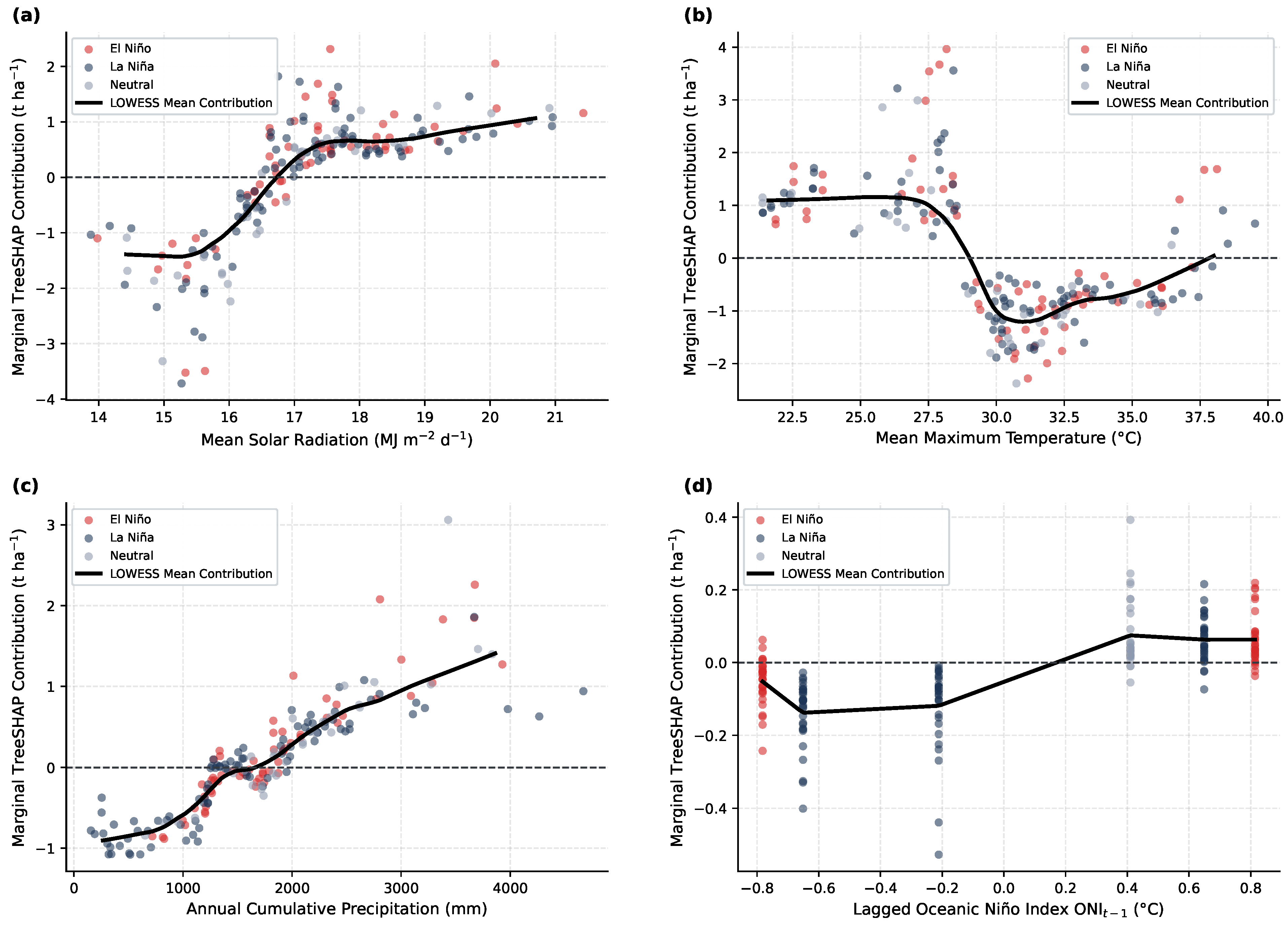
verifying additive reconstruction within absolute tolerance. Lagged yield is omitted from this specification by design: because it carries each department’s productive level, it dominates the attributions and leaves little to attribute to climate, whereas the question here is how climate enters when productive history is unavailable. As a sensitivity analysis, the same held-out attributions are computed for the dynamic XGBoost specification that adds . For visual description only, LOWESS smoothers [40] (nominal span 0.38 across a 120-point grid between the 2nd and 98th predictor percentiles) are fitted to predictor–attribution pairs, averaging attributions that share a predictor value. Zero-attribution crossings are not estimated or interpreted: they depend on the fitted model, the smoothing span, and the predictor range, and they do not correspond to physiological thresholds or any mechanistic process.
3.6. Descriptive Resilience Indicators
The distinction between stability, resistance, and recovery follows the conceptual literature on agricultural and ecological resilience [41,42]. We use study-specific descriptive thresholds and ratios rather than treating them as validated measures from those sources. Department–years satisfying , , or °C are flagged. For each department i, let denote flagged years with valid positive yields across the contiguous three-year window . Departmental resistance () and recovery () are defined as the medians of the adjacent-year yield ratios:
supplemented by the two-year ratio . Multi-year detrended stability is computed from Theil–Sen residuals as
where and is the residual standard deviation. After min–max normalizing the rounded departmental summaries of , , and to , a descriptive composite score is calculated as .
3.7. Reproducibility
The workflow uses fixed analysis settings and a pseudorandom seed of 42. Input data integrity is verified before and after execution via SHA-256 checksums, and automated checks verify zero-window Euclidean equivalence (), recovery of a synthetic temporal shift, and strict out-of-time cohort alignment. Analysis settings, predictions, and validation results are retained to support reproducibility.
4. Results and Discussion
The results distinguish whole-trajectory departmental profiles from annual yield-state mobility. Climate prediction, model explanation, and event-window ratios complement this characterization.
4.1. Scale-vs.-Shape Typology
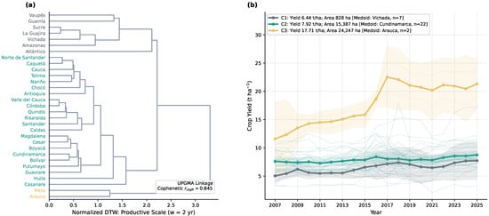
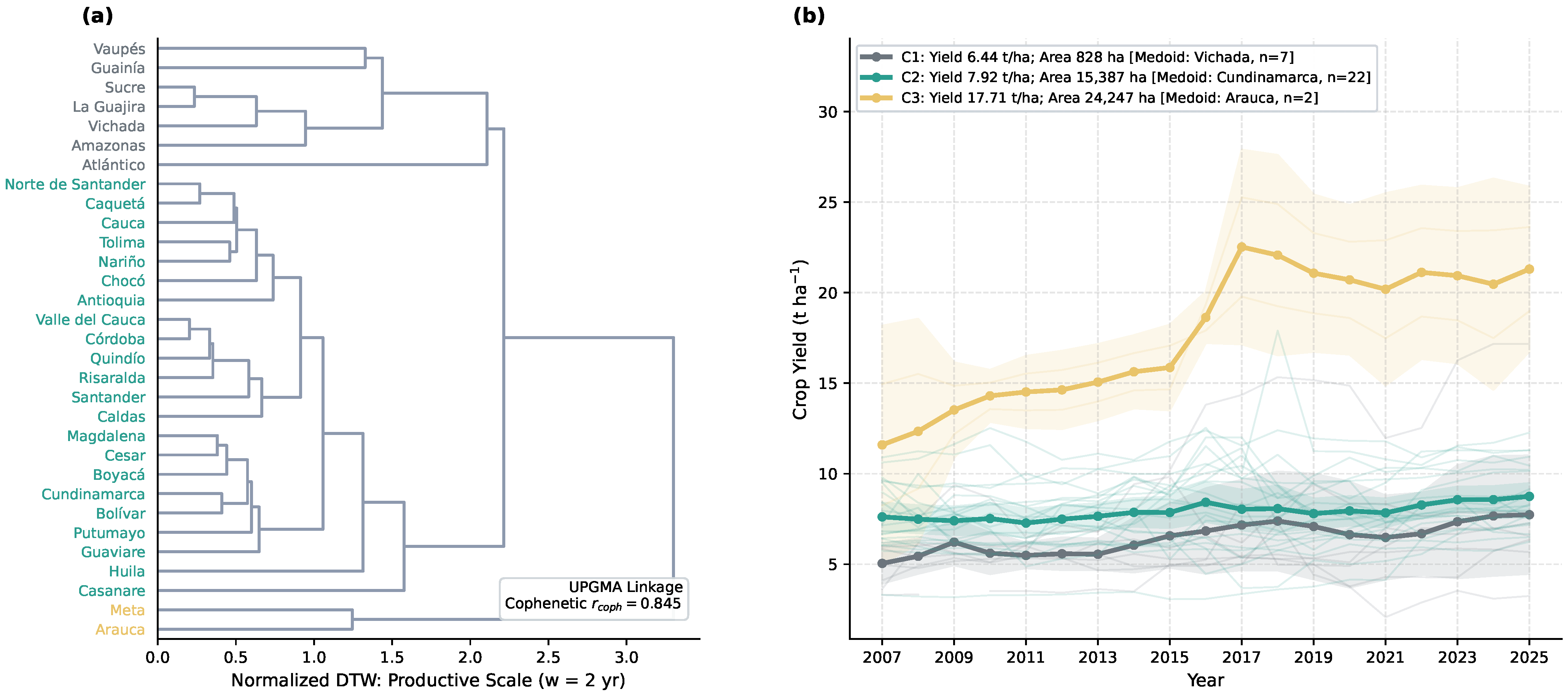
Across all 465 departmental pairs, trajectory distances use 18 or 19 shared observed years. The three-group PAM production-scale typology combines differences in yield and harvested area (Table 1; Figure 2). The group mean of departmental yields (Table 1 reports medians) ranges from in , seven departments with small harvested areas, to in , the Arauca–Meta pair; the remaining 22 departments form . The Arauca–Meta pair also has the highest mean Sen slope (), the largest mean area, and the lowest mean detrended residual CV. These are summaries of the variables defining the clusters, rather than independent validation of three regimes.
Table 1.
Three-group PAM production-scale typology (, ). (a) Distributions of departmental means; for the range spans its two departments. (b) Effect sizes and for all variables. Yield and area define the clusters, so no p values are reported for them; p values for the five climate variables are exploratory, with Holm adjustment across the five in parentheses.
Figure 2.
Bivariate production-scale DTW analysis (). (a) Auxiliary UPGMA dendrogram, with terminal labels colored by PAM group. (b) Annual group mean yields, individual trajectories, and descriptive standard-error bands.
Differences in yield and area between groups are large by construction ( for mean yield and for lagged area) and do not validate the clusters. The climate comparisons are exploratory: maximum temperature differs between groups at unadjusted (Kruskal–Wallis ; ANOVA ; ) but not after Holm adjustment (), and the other climate means differ little (; unadjusted ). These exploratory comparisons do not rule out associations within departments or at finer temporal scales.
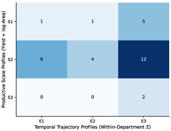
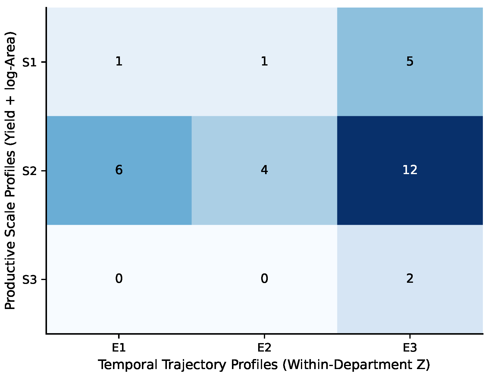
The three-group scale and shape assignments have little agreement (; Figure 3). However, the limited separation of the shape solutions prevents interpreting this disagreement as evidence for a second set of well-defined temporal regimes.
Figure 3.
Cross-tabulation of department counts between production-scale clusters (rows, labeled – in the figure for clusters –) and trajectory-shape clusters (columns, –). These row labels are distinct from annual Markov states. Cell shading is proportional to the number of departments, with darker cells indicating more departments.
4.2. Temporal Alignment and Cluster Stability
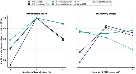
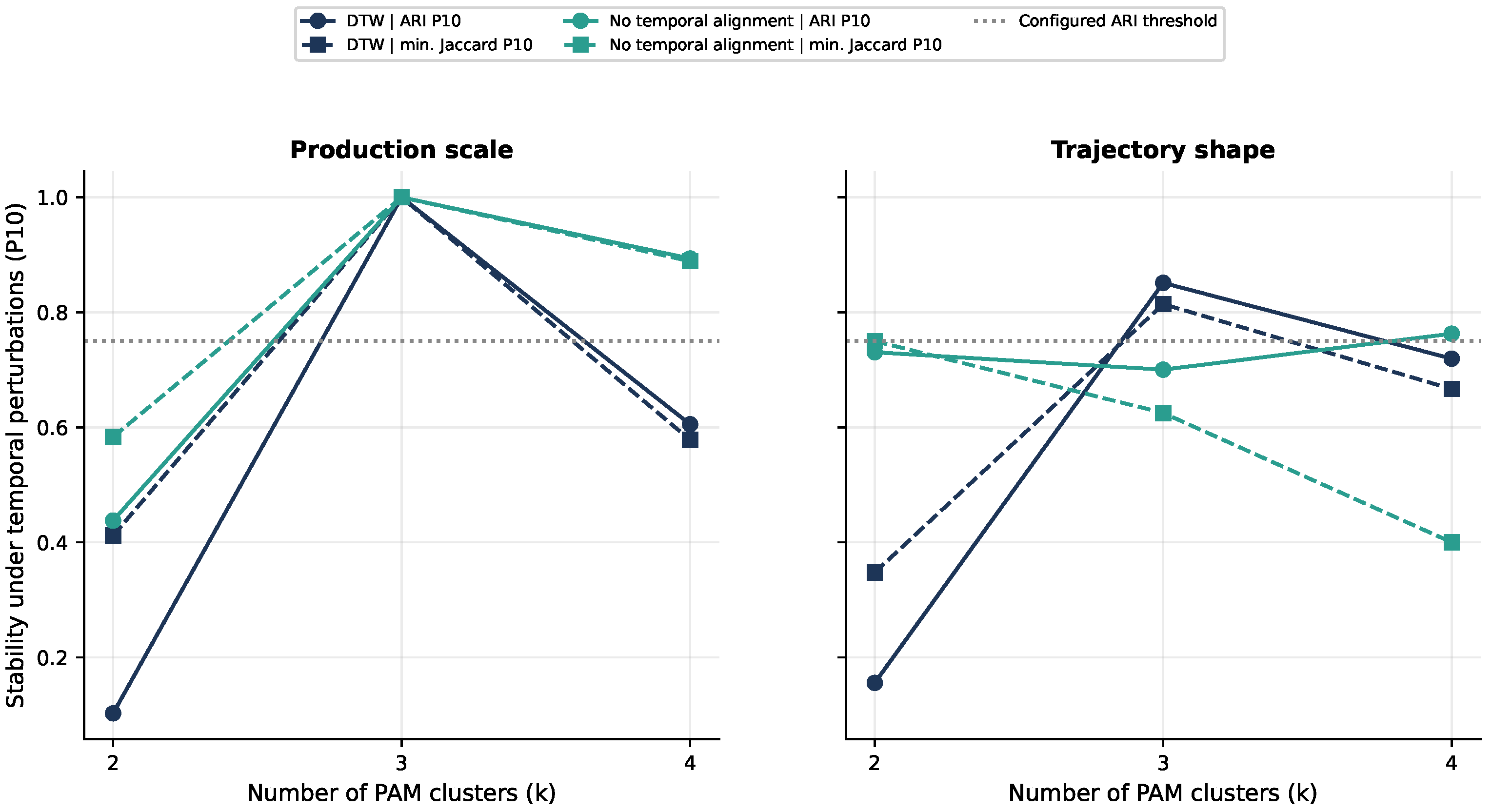
For the three-group scale solution, DTW and synchronous RMS recover the same full-period partition and both reach ARI P10 and minimum-group Jaccard P10 of 1.000 (Table 2). Mean perturbation ARI is 1.000 for DTW and 0.972 for synchronous RMS. Thus DTW preserves this partition across all 37 removals, while the synchronous solution changes in a minority of removals; equality at P10 alone masks this difference. These diagnostics support robustness of the three-group solution under both distances, rather than a general superiority of DTW. The static reference based only on departmental means reproduces this partition exactly (ARI with both distances), with mean ARI and ARI P10 across the same removals. The solution therefore reflects persistent differences in productive level, and its stability does not show added value from modeling trajectories or temporal alignment.
Table 2.
PAM sensitivity across 37 year-removal perturbations. (a) Distances and geometries; minimum Jaccard P10 is , and common-year ARI uses the 18 years observed by all departments. (b) Production-scale partition with under other DTW windows (equal weights) and yield weights (log-area receives the remainder; ); ARI vs. reference compares with the retained partition, and silhouettes are computed within each weighted distance, so they are not directly comparable across rows.
As a sensitivity analysis, the four-group DTW scale partition falls below the ARI and Jaccard thresholds (0.605 and 0.578), whereas the synchronous partition satisfies the operational criteria (0.894 and 0.889). The Arauca–Meta pair remains separate in both four-group solutions, but other departments are reassigned between distances. Four-group profiles are therefore not used for the main results. Other production-scale DTW candidates also satisfy the criteria, including PAM with and (silhouette 0.274 and 0.291) and two-group average and complete linkage (silhouette 0.551), which only separates Arauca and Meta from the remaining departments; these results do not establish an optimal number of groups. Varying the DTW window from 0 to 4 years leaves the three-group partition unchanged (ARI with the reference; silhouette 0.478–0.493), whereas the four-group solution meets the criteria only for and (not tabulated; Table 2b lists ). The relative weight of yield and log-area matters much more. With yield weights of 0, 0.25, 0.75, and 1, the three-group partition agrees with the reference at ARI 0.301, 0.301, 0.128, and 0.099, respectively, and fails the criteria at a yield weight of 0.75. Arauca and Meta remain a separate pair whenever yield receives at least half of the weight, but the composition of the other groups changes. The retained typology therefore describes the joint scale of yield and harvested area under equal weighting rather than a classification that holds across weightings. No evaluated shape partition satisfies all criteria: separation is below the silhouette threshold even when some stability measures are relatively high (Table 2a; Figure 4).
Figure 4.
PAM sensitivity under DTW () and synchronous RMS () for , across production scale (left) and trajectory shape (right), using 37 deterministic year-removal perturbations.
4.3. Similarity Network and Departmental Trends
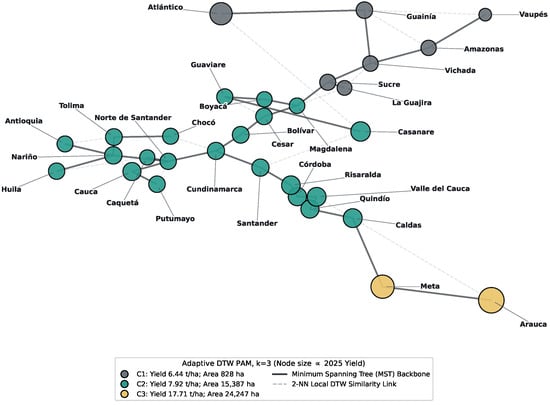
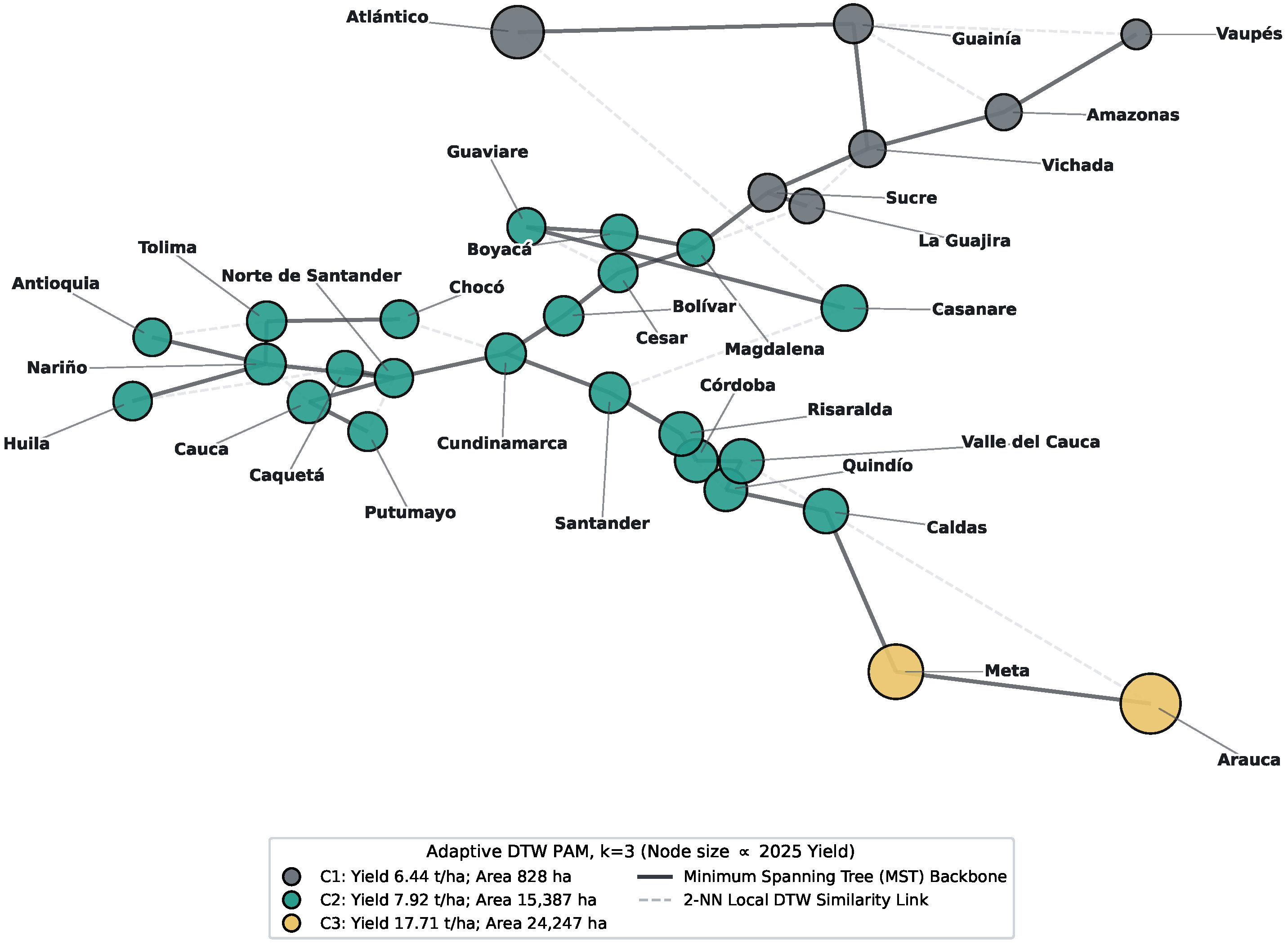
In the MST ∪ 2-NN similarity graph, Cundinamarca has the highest shortest-path betweenness (0.6460, degree 4), followed by Cesar (0.4276, degree 4) and Santander (0.4161, degree 3; Figure 5). These centralities describe positions in the selected similarity graph, without establishing physical connections, trade flows, or spatial spillovers.
Figure 5.
Departmental DTW similarity network (MST ∪ 2-NN). Colors indicate PAM production-scale groups; node size is proportional to observed yield in 2025.
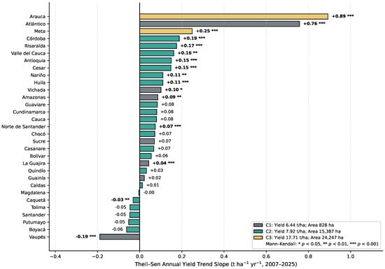
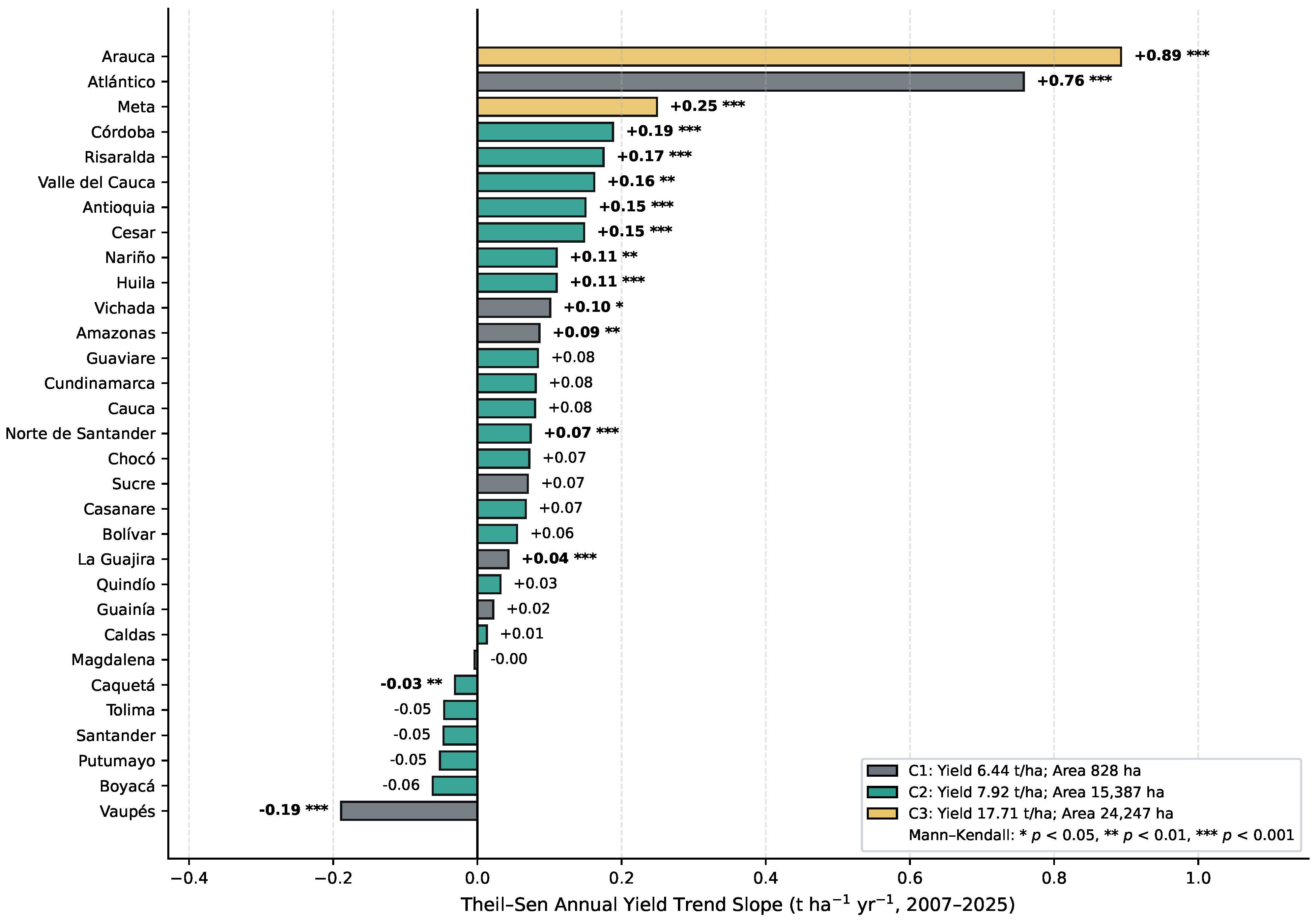
Ordinary Mann–Kendall tests detect 14 positive and two negative yield trends before multiplicity adjustment. After Holm adjustment, 12 positive and two negative trends remain (Table 3; Figure 6). Arauca and Atlántico have the largest positive Sen slopes ( and ). Caquetá and Vaupés have negative adjusted trends. Risaralda combines yield growth () with decreasing harvested area (). None of these trends identifies its agronomic or institutional cause, and the ordinary tests do not adjust for serial dependence.
Table 3.
Departments with Holm-adjusted yield trends (). Sen slopes are in t ha−1 yr−1. Significance is exploratory because the ordinary test does not correct serial dependence.
Figure 6.
Departmental Sen yield slopes colored by PAM group. Asterisks indicate unadjusted Mann–Kendall ; Table 3 lists Holm-adjusted trends.
4.4. Yield-State Persistence and Conditional Markov Quantities
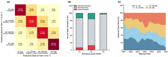
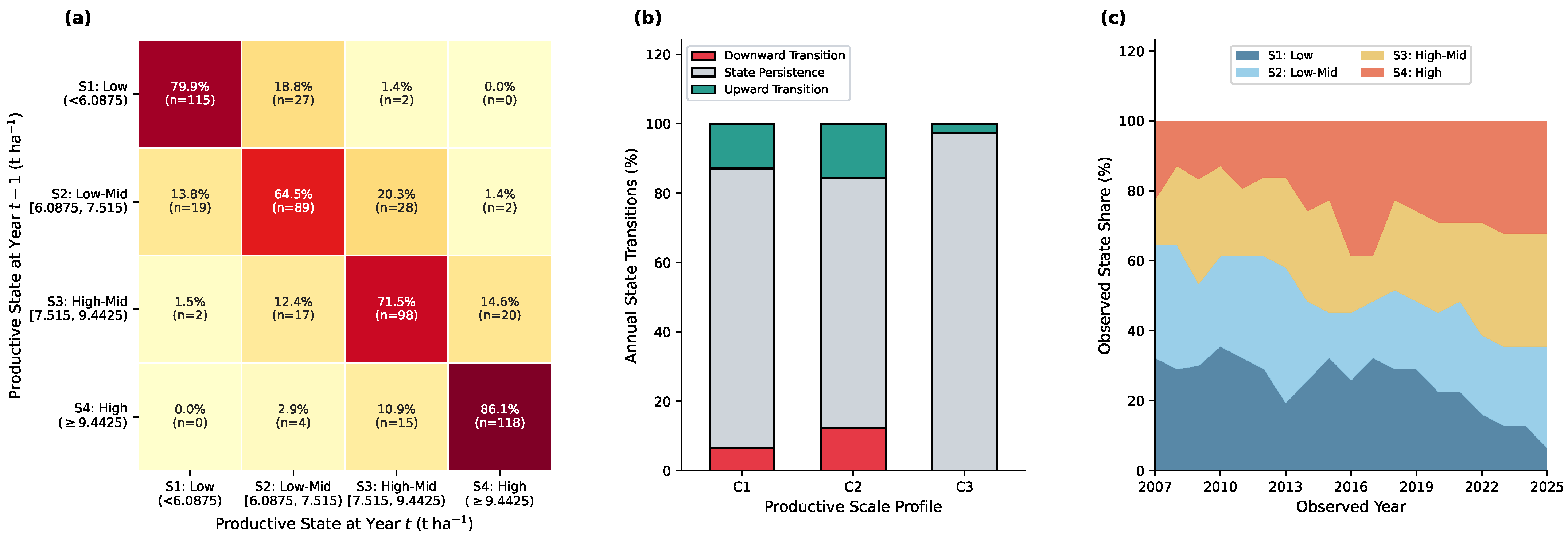
Pooled quartile boundaries are , , and . Across 556 consecutive annual transitions, 420 remain in the same state (), 79 move upward (), and 57 move downward (). Retention is in and in (Table 4; Figure 7). No single-year jump between the extreme states is observed; zero observed counts do not establish that such jumps are impossible.
Table 4.
Annual yield-state transitions. (a) Observed counts and row-normalized MLE probabilities: each cell reports (row percentage), N is the outgoing-transition total, and boundaries are in t ha−1 at the full precision displayed. (b) Observed retention compared with 10,000 permutations of years within departments; rows are origin states and rows are trajectory clusters. (c) Asymptotic and simulation-calibrated p values under first-order chains with a common matrix (Null A) or department-specific shrunk matrices (Null B). (d) Sensitivity of pooled long-run quantities and retention to the resampling design and to re-estimating the quartile boundaries; the passage time is the mean first passage time.
Figure 7.
Markov summaries: (a) pooled MLE transition matrix; (b) observed retention and upward/downward mobility by trajectory group; (c) observed annual state shares. Yield states and trajectory groups are different classifications.
Observed retention exceeds the within-department null overall ( vs. ; ) and in every origin state and cluster (Table 4b). Stable departmental state frequencies therefore account for a large share of retention, but not all of it: the null alone reaches in and in . Because permutation removes all temporal order, the excess may reflect within-department trends and step changes as well as year-to-year persistence.
Transitions also differ across groups. The heterogeneity statistic is (df ; permutation ) among clusters and (df ; ) among departments, with differences among departments within (; df ; ) and (; df ; ); the contrast within is not estimable because Meta remains in a single state. Departmental retention ranges from in Guaviare to in Caldas, Casanare, La Guajira, and Meta. Of the 27 departments visiting more than one state, 19 exceed their own null at unadjusted , and 12 of the 31 departments do so after Holm adjustment. The pooled matrix is therefore an average across heterogeneous departments rather than evidence of a common dynamic process.
The empirical transition graph is irreducible and aperiodic, with a spectral gap of 0.1273. Comparing subperiods up to 2015 and after 2015 gives () and (), and calibration does not change this conclusion (Table 4c). However, the split at the 2018 source boundary rejects homogeneity (; df ; calibrated ), with retention rising from to . The data cannot separate a real change from a change in reporting. Three further checks address this boundary. First, the panel reproduces Agronet’s published values for the domestic-consumption subcategory in all 589 department–years and matches the sums of the corresponding municipal records within 1% for 334 of 341 department–years in 2007–2017 and for all 217 in 2019–2025, but for none of the 31 departments in 2018. The 2018 values published by Agronet therefore do not come from the same release as the Ministerio’s open municipal base. Second, a regression with department fixed effects and department-specific linear trends shows no significant level shift at 2019 (log yield , SE , ; log area , ), and none of the 14 candidate breaks between 2010 and 2023 is significant for either variable, although the 2019 break has the second-largest absolute t statistic for log yield, after 2018. Third, excluding the transitions into 2018 and 2019 does not remove the change in transitions: homogeneity is still rejected (; df ; asymptotic ), with retention before and after. The number of municipalities reporting plantain changes little (771 in 2018 and 784 in 2019). Because neither version of the 2018 values can be verified, the Markov analysis was repeated with two alternative panels, re-estimating the quartile boundaries in each: replacing the 31 values for 2018 with yields computed from the Ministerio’s municipal records, which changes the 2018 state of 14 departments, and treating 2018 as missing. Retention is and , against in the reference panel; the within-department null gives and ( in both); the stationary share of is and against ; and the mean first passage time from to is and years against . The descriptive Markov summaries therefore do not depend on which 2018 values are used. The homogeneity test at the 2018 boundary does: with the municipal values it is no longer rejected at the 0.05 level (; df ; asymptotic ; retention before and after), whereas it is rejected with the reference values and when 2018 is excluded. The evidence for a change in transitions after 2018 is therefore sensitive to the 2018 values and remains uncertain. Calibration matters for sparse counts: 44 of the 64 second-lag cells contain fewer than five transitions, and the statistic averages under Null A against 26 nominal degrees of freedom.
The one-lag assumption is not established. Retention is when the state at equals the state at and otherwise, and the second-lag statistic rejects Null A (; df ; ). Under department-specific chains, the result depends on the shrinkage setting ( for and for ), so this dependence cannot be separated from departmental differences with about 18 transitions per department. A Bayesian information criterion comparison based on the pooled likelihood ratio still favors the first-order model by because of the 26 added parameters. Duration shows the same pattern: the probability of leaving a state falls from after one year to after four or more years, with no exits in 35 such transitions from (; df ; Null A ; Null B and ). The first-order pooled chain is therefore a descriptive summary, not a validated data-generating model.
Under the pooled MLE matrix, stationary shares are 16.91%, 21.68%, 28.81%, and 32.60%. Dirichlet smoothing () changes them by at most 0.94 percentage points. Long-run uncertainty remains wide: the two-way bootstrap interval for is 10.3–67.3%, and the mean first passage time from to is 24.60 years (interval 15.7–68.1). These are quantities conditional on the pooled transition model, not observed convergence times or expectations for any particular department. The interval widths are not driven by the resampling design alone (Table 4d). With moving blocks of two, three, and five years, the interval for is –, –, and –, and the upper limit of the -to- passage time falls from to , , and years. Re-estimating the boundaries gives – and – years, with 95% ranges of –, –, and – for the three boundaries. Resampling only departments or only years gives narrower intervals because the other source of variation is held fixed. Retention remains between and across the two-way and blocked variants, so long-run quantities remain weakly determined under every design.
4.5. Incremental Climate Prediction and Model Explanation
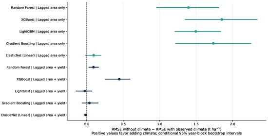
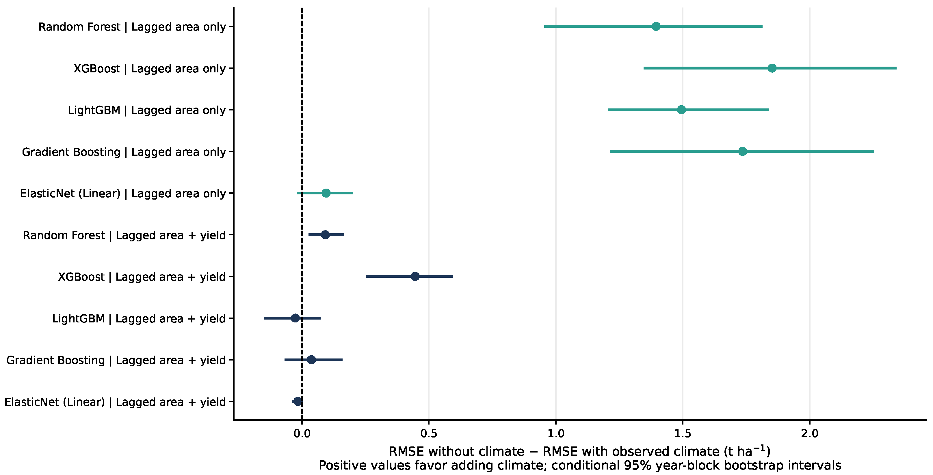
On the 186 held-out observations, adding climate to lagged area lowers pooled RMSE in all five algorithms (Table 5; Figure 8). Reductions in the four tree ensembles range from to ; ElasticNet improves by . Although all four tree models show lower annual MAE in each test year, none of the ten paired comparisons is statistically significant after Holm adjustment (). These reductions are therefore descriptive. Because the tests use six annual differences, the smallest attainable two-sided Wilcoxon p value is , or after Holm adjustment across ten comparisons, so significance at the 0.05 level was not attainable. The bootstrap intervals address a different estimand, the pooled RMSE gain, and their year-block version also rests on six test years.
Table 5.
Paired climate comparisons (2020–2025; ). RMSE and ΔRMSE are in t ha−1; positive gain favors climate. (a) Brackets give conditional 95% year-block bootstrap intervals for the pooled RMSE gain; Holm-adjusted p values refer to annual MAE differences, a different estimand. (b) Conditional 95% intervals for the same pooled RMSE gain, resampling departments or departments and years crossed. (c) Pooled RMSE gains (t ha−1) when the climate vector is replaced by permuted years within departments, departmental training means, or coordinates alone.
Figure 8.
Pooled RMSE gains from adding observed climate under area-only and area-plus-yield baselines, with conditional 95% year-block bootstrap intervals.
With lagged yield included, climate lowers pooled RMSE in three models: by 10.2% for Random Forest, 32.7% for XGBoost, and 4.0% for Gradient Boosting, whereas the error increases for LightGBM and ElasticNet. The conditional year-block intervals exclude zero for Random Forest and XGBoost (gains) and for ElasticNet (loss). These intervals depend on the resampling unit (Table 5b). With lagged area alone, the four tree models still exclude zero under department and crossed resampling. With lagged yield, department resampling still excludes zero for Random Forest and XGBoost and for the ElasticNet loss, but crossed department–year resampling excludes zero only for XGBoost.
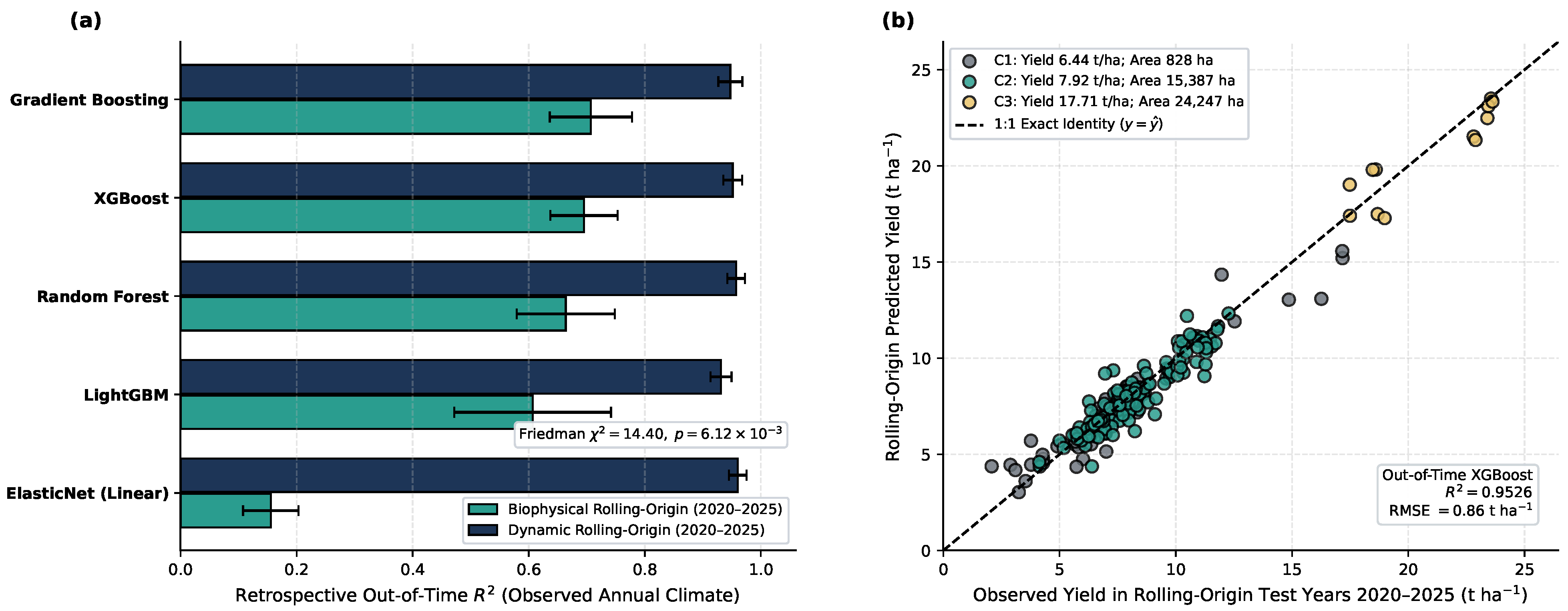
Table 5c indicates that the large gains without lagged yield come from fixed location rather than annual climate. With climate years permuted within departments, the four tree models gain – t ha−1 on average, similar to the observed –, and training climate means or coordinates alone give larger gains (–). With lagged yield, observed climate does not outperform all 20 permutations for any model; at least 3 of the 20 permutations perform as well in every case. Climate variables therefore act mainly as identifiers of the reference points in these retrospective comparisons, and the annual climate signal is small at best. These differences vary by algorithm and are not statistically significant after Holm adjustment (Table 5). In addition (Figure 9), persistence has the lowest pooled RMSE (), below the best climate-augmented model (). This comparison concerns retrospective prediction in known departments, not causal climate effects or ex ante forecasting. Pooled performance also combines between-department differences and within-department changes.
Figure 9.
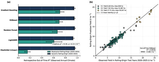
Separate rolling-origin benchmark: (a) mean annual under biophysical and dynamic specifications; (b) pooled observed vs. predicted yields for dynamic XGBoost. Error bars in (a) show the standard deviation of across the six test years, and the Friedman statistic compares annual MAE across the five models. Feature ordering in the dynamic benchmark differs from the paired comparisons in Table 5; the fitted stochastic models need not be identical.
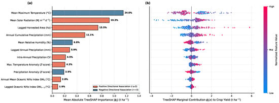
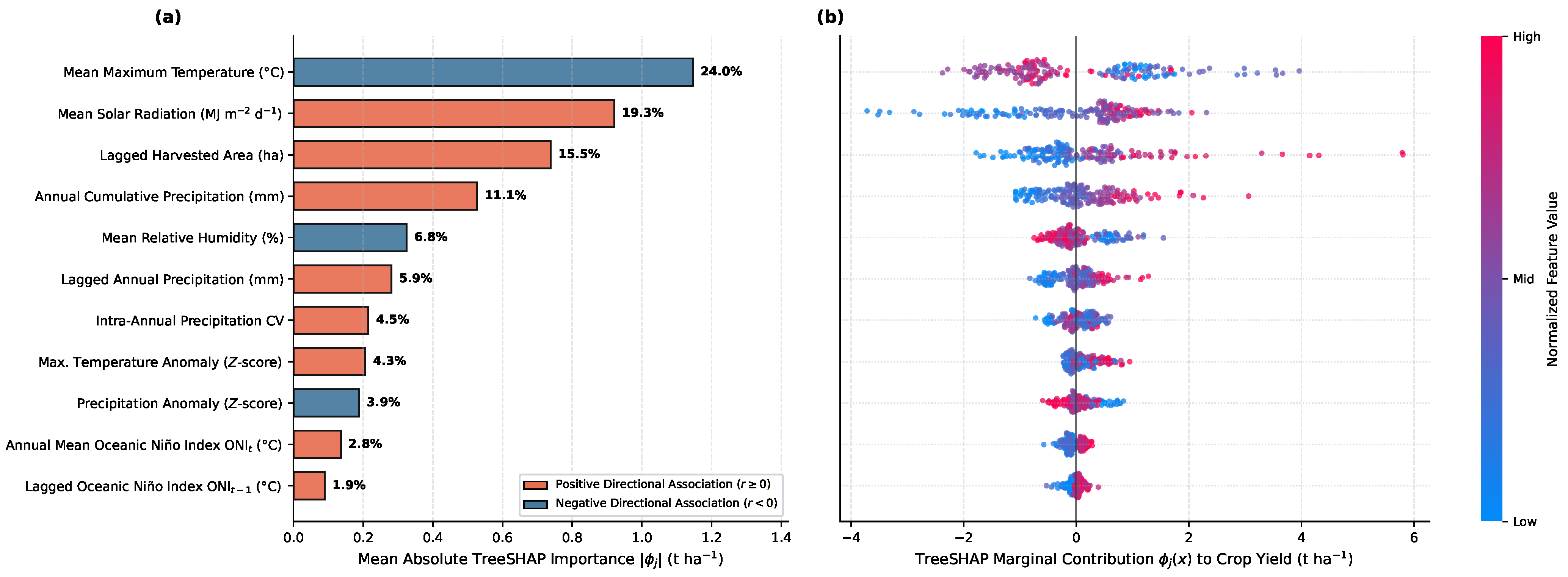
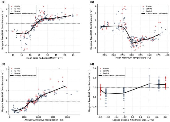
In the held-out biophysical XGBoost explanations, maximum temperature (24.00%), radiation (19.29%), and lagged area (15.46%) account for of total mean absolute attribution (Table 6; Figure 10). Predictor–attribution correlations for radiation and maximum temperature are and , and the LOWESS curves are shown only to describe the fitted model (Figure 11). These are model-specific associations. Annual precipitation has a variance inflation factor of 7.73, and the pooled explanations combine spatial and temporal variation. Because radiation and maximum temperature vary mainly between reference points, their attributions also reflect differences between locations. When lagged yield is included, it accounts for of total mean absolute attribution, the climate variables together fall from to , and radiation and maximum temperature fall to and . Differences between departments explain of the variance in the lagged-yield attributions. The biophysical attributions therefore describe a model without productive history and should not be read as the drivers of the best predictions.
Table 6.
Out-of-time TreeSHAP summary for biophysical XGBoost (). Share is the percentage of total mean , and is the correlation between each predictor and its attribution.
Figure 10.
Out-of-time TreeSHAP attributions for the biophysical XGBoost specification: (a) mean absolute importance and (b) instance-level attribution distributions.
Figure 11.
LOWESS curves of held-out TreeSHAP attributions for (a) radiation, (b) maximum temperature, (c) annual precipitation, and (d) lagged ONI. Points are coloured by the ENSO phase of year t. Curves are descriptive summaries of the fitted model; no zero-attribution crossings are estimated.
4.6. Descriptive Shock Response and Study Limitations
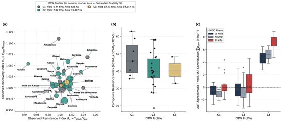
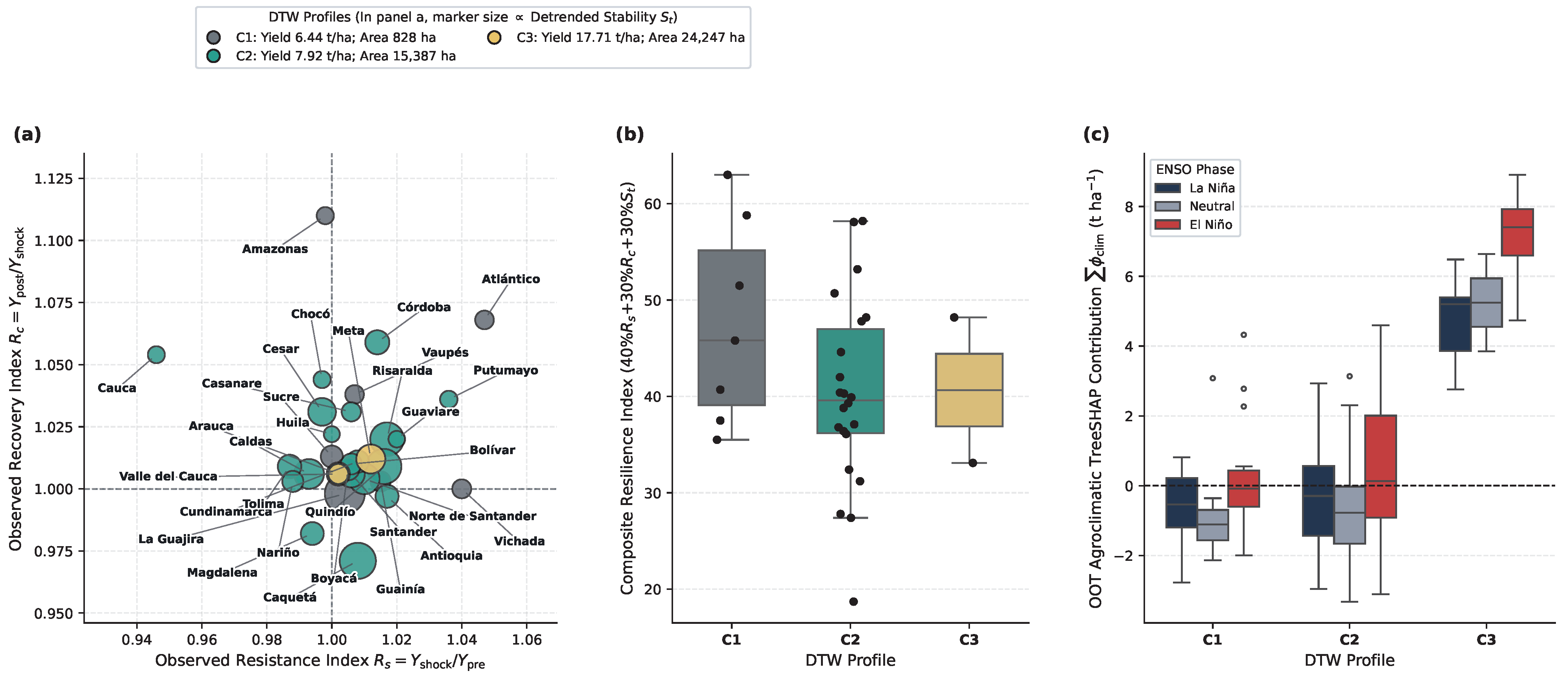
Between 7 and 12 valid three-year anomaly windows occur per department. La Guajira has the highest detrended stability (), reflecting small residual dispersion around its estimated trend. Atlántico has the highest composite score (), with , , and (Figure 12). Adjacent-year ratios can reflect an underlying growth trend and overlapping anomalies, so they do not isolate resistance or recovery caused by a particular climatic event. The composite ranking also depends on the chosen weights.
Figure 12.
Descriptive shock-response and attribution synthesis: (a) resistance and recovery ratios, with marker size proportional to detrended stability; (b) composite scores by DTW group; (c) net held-out climatic TreeSHAP attributions by group and ENSO phase.
The interpretation is limited by departmental aggregation, single-point climate proxies, and only six out-of-time test years. Climate is not weighted by crop location and annual summaries do not resolve sensitive growth stages. Annual summaries match the resolution of the yield records, which aggregate continuous harvests from plantings of different ages, but they cannot represent conditions during flowering or bunch filling. The reference points are also uncertain proxies: NASA POWER and CHIRPS precipitation differ by more than 25% in mean annual total at 14 of the 31 points, their correlation across years is 0.50 or lower at 20 points (median ), and their departmental means correlate at (Table A1). Caldas and Risaralda, and Quindío and Valle del Cauca, fall in the same NASA POWER grid cells and therefore share identical climate series. In large departments such as Meta and Arauca, a single reference coordinate may miss microclimatic variation across the actual growing areas, and this spatial mismatch could distort the TreeSHAP rankings in Table 6. Over the 2020–2025 evaluation years, differences among the reference points account for of the variance in annual radiation and of that in maximum temperature, so the prominence of these predictors may largely reflect contrasts between fixed locations rather than climatic responses within departments. Sparse Markov cells, limited temporal replication, the change of source label after 2018 and the 2018 values, which differ between Agronet and the municipal records and could not be verified, and unresolved second-lag and duration dependence constrain inference, while pooling departments averages over transitions that differ among departments. Because Markov states use nationally pooled quartiles, departments with persistently high or low yields are structurally confined to upper or lower states, so retention reflects fixed differences in productivity as well as inter-annual persistence: Caldas, Casanare, La Guajira, and Meta remain in a single state throughout, and 15 of the 31 departments visit at most two states. As a sensitivity check, randomly permuting the years within each department (10,000 permutations), which preserves its state composition but removes temporal order, still yields mean retention of overall (95% range 51.98–58.27%), in , and in , compared with the observed , , and . The observed retention should therefore not be read as inter-annual persistence alone, and the excess above these permutation values may also include within-department trends. Ordinary trend tests do not adjust for serial dependence. The panel covers plantain for domestic consumption and excludes export plantain, reported in six departments and mostly in Antioquia (66.9% of the cumulative harvested area of export plantain), so the results do not describe the export sector. Finally, records contain no direct measures of cultivars, irrigation, fertilization, or pest control: neither the profiles nor the model attributions establish technological adoption or causal mechanisms. The weaker separation of normalized shape solutions further limits claims about distinct temporal regimes.
5. Conclusions and Future Work
The departmental records reveal productive heterogeneity and persistent annual yield states. Three-group scale partitions are robust under both DTW and synchronous distance, while DTW maintains the reference partition across all tested year removals. This partition is reproduced by departmental means alone, so it describes persistent differences in productive level rather than distinct temporal trajectories. The four-group DTW solution fails the stability criteria and is reported only as a sensitivity analysis. The partition is insensitive to the DTW window but changes when yield and area are weighted unequally. The high-yield Arauca–Meta profile does not establish a distinct technological regime, and normalized shape solutions do not support a firm classification of departments by temporal evolution alone.
Of the observed annual transitions, 75.54% remain within the same yield quartile. This retention exceeds the 55.06% expected from each department’s state frequencies alone, but transitions differ across departments, so the pooled chain summarizes an average rather than a common dynamic process. Calibrated tests also reject a common first-order chain for second-lag and duration dependence, so one lag is not established as sufficient. The pooled Markov summaries are robust to replacing or omitting the inconsistent 2018 values, whereas the rejection of temporal homogeneity at the 2018 source boundary is not. Adding climate lowered pooled RMSE relative to lagged area and in several models with lagged yield, but location alone reproduces most of these reductions. The differences were not statistically significant after Holm adjustment, and no climate-augmented model outperformed the persistence baseline in pooled RMSE.
With only six evaluation years, statistical power is limited and the annual tests could not reach significance, so these results neither establish nor rule out a climate contribution. These findings concern retrospective prediction at departmental scale; they do not imply that climate is agronomically unimportant. TreeSHAP, event-window ratios, and long-run Markov quantities retain their conditional interpretations.
Future work should examine longer or finer-scale panels, crop-location-weighted sub-seasonal weather, and direct management covariates. Independent temporal evaluation could test whether the exploratory profiles persist and whether climate information improves prediction beyond simple productive-history baselines.
Author Contributions
Conceptualization, R.G.; methodology, R.G.; validation, J.P.; formal analysis, R.G.; investigation, J.P.; resources, A.D.; data curation, A.D.; writing—original draft preparation, R.G.; visualization, A.D.; supervision, J.P.; project administration, J.P. All authors have read and agreed to the published version of the manuscript.
Funding
This research received no external funding.
Data Availability Statement
The agricultural data source is Agronet’s departmental statistics [19]. The study data and computational implementation are publicly available at https://github.com/devraxielh/Plantain-trajectories-colombia (accessed on 8 November 2026).
Conflicts of Interest
The authors declare no conflict of interest.
Appendix A. Climate Reference Points
Table A1.
Reference points used to retrieve NASA POWER data: the municipal seat (DIVIPOLA) of the municipality with the largest cumulative production of domestic-consumption plantain in 2007–2025, with its share of departmental production. Mean annual precipitation from NASA POWER and CHIRPS v2.0 at the same point (2007–2025) and their correlation across years are also shown. Each department is represented by a single point, not weighted by crop location.
References
- Zartha Sossa, J.W.; Gutiérrez Posada, N.; Zuluaga Monsalve, A.M.; Botero Montoya, L.H.; Gutiérrez Cano, L.F.; González Candia, J.; Gómez Salazar, J.O.; Orozco Mendoza, G.L.; Escobar Mora, N.J. Sustainable Innovation Management Model (MGI) for Plantain Agroindustrial Chain. Sustainability 2025, 17, 1716. [Google Scholar] [CrossRef] [Scilit]
- Parra-Londono, S.; Tigreros, J.A.; Montoya-Correa, C.A. Colombian Crop Resilience: Evaluating National Yield Stability for Fruit and Vegetable Systems. Agriculture 2024, 14, 1546. [Google Scholar] [CrossRef] [Scilit]
- Sakoe, H.; Chiba, S. Dynamic programming algorithm optimization for spoken word recognition. IEEE Trans. Acoust. Speech Signal Process. 1978, 26, 43–49. [Google Scholar] [CrossRef] [Scilit]
- NASA POWER. Monthly and Annual API (Application Programming Interface). Available online: https://power.larc.nasa.gov/docs/services/api/temporal/monthly/ (accessed on 22 October 2026).
- NOAA Climate Prediction Center. Cold and Warm Episodes by Season (ERSSTv6). Available online: https://www.cpc.ncep.noaa.gov/products/analysis_monitoring/enso/oni/v6/ (accessed on 23 October 2026).
- Blasch, G.; Li, Z.; Taylor, J.A. Multi-temporal yield pattern analysis method for deriving yield zones in crop production systems. Precis. Agric. 2020, 21, 1263–1290. [Google Scholar] [CrossRef] [Scilit]
- de Souza, E.G.; Khosla, R.; Sudduth, K.A.; Johann, J.A.; Bazzi, C.L. Spatial and Temporal Variability in Yield Maps Can Localize Field Management—A Case Study with Corn and Soybean. Agronomy 2025, 15, 1179. [Google Scholar] [CrossRef] [Scilit]
- Scudiero, E.; Teatini, P.; Manoli, G.; Braga, F.; Skaggs, T.H.; Morari, F. Workflow to Establish Time-Specific Zones in Precision Agriculture by Spatiotemporal Integration of Plant and Soil Sensing Data. Agronomy 2018, 8, 253. [Google Scholar] [CrossRef] [Scilit]
- Rodas-Vásquez, A.; Castillo-Rodriguez, C.M.; Bermúdez-Edo, M.; Molina-Cabrera, A.; Chavarro-Porras, J.C.; Meneses-Escobar, C.A. Nutrient recommendation model for plantain (Musa AAB) cultivation based on the analysis of soil variables in the Department of Risaralda, Colombia. J. Saudi Soc. Agric. Sci. 2026, 25, 6. [Google Scholar] [CrossRef] [Scilit]
- Javed, A.; Lee, B.S.; Rizzo, D.M. A benchmark study on time series clustering. Mach. Learn. Appl. 2020, 1, 100001. [Google Scholar] [CrossRef] [Scilit]
- Holder, C.; Middlehurst, M.; Bagnall, A. A review and evaluation of elastic distance functions for time series clustering. Knowl. Inf. Syst. 2024, 66, 765–809. [Google Scholar] [CrossRef] [Scilit]
- Li, H.Y.; Lawarence, J.A.; Mason, P.J.; Ghail, R.C. Fast Dynamic Time Warping and Hierarchical Clustering with Multispectral and Synthetic Aperture Radar Temporal Analysis for Unsupervised Winter Food Crop Mapping. Agriculture 2025, 15, 82. [Google Scholar] [CrossRef] [Scilit]
- Huzsvai, L.; Kovács, E.; Tuba, G.; Juhász, C.; Jug, D.; Zsembeli, J. Discrete-Time Markov Chain Method for Predicting Probability of Crop Yield Variability. Earth 2025, 6, 142. [Google Scholar] [CrossRef] [Scilit]
- Varma, V.; Bebber, D.P. Climate change impacts on banana yields around the world. Nat. Clim. Change 2019, 9, 752–757. [Google Scholar] [CrossRef] [Scilit] [PubMed]
- Huber, F.; Yushchenko, A.; Stratmann, B.; Steinhage, V. Extreme Gradient Boosting for yield estimation compared with deep learning approaches. Comput. Electron. Agric. 2022, 202, 107346. [Google Scholar] [CrossRef] [Scilit]
- Lundberg, S.M.; Erion, G.; Chen, H.; DeGrave, A.; Prutkin, J.M.; Nair, B.; Katz, R.; Himmelfarb, J.; Bansal, N.; Lee, S.I. From local explanations to global understanding with explainable AI for trees. Nat. Mach. Intell. 2020, 2, 56–67. [Google Scholar] [CrossRef] [Scilit] [PubMed]
- Ministerio de Agricultura y Desarrollo Rural. Evaluaciones Agropecuarias Municipales EVA. Datos Abiertos Colombia. Available online: https://www.datos.gov.co/Agricultura-y-Desarrollo-Rural/Evaluaciones-Agropecuarias-Municipales-EVA/2pnw-mmge (accessed on 7 November 2026).
- Unidad de Planificación Rural Agropecuaria. Evaluaciones Agropecuarias Municipales—EVA. 2019–2025. Base Agrícola. Datos Abiertos Colombia. Available online: https://www.datos.gov.co/Agricultura-y-Desarrollo-Rural/Evaluaciones-Agropecuarias-Municipales-EVA-2019-20/uejq-wxrr (accessed on 7 November 2026).
- Unidad de Planificación Rural Agropecuaria. Área, Producción y Rendimiento Departamental. AgroNET. Available online: https://agronet.gov.co/estadisticas/agricola#departamental (accessed on 22 October 2026).
- Funk, C.; Peterson, P.; Landsfeld, M.; Pedreros, D.; Verdin, J.; Shukla, S.; Husak, G.; Rowland, J.; Harrison, L.; Hoell, A.; et al. The climate hazards infrared precipitation with stations—A new environmental record for monitoring extremes. Sci. Data 2015, 2, 150066. [Google Scholar] [CrossRef] [Scilit] [PubMed]
- Kaufman, L.; Rousseeuw, P.J. Partitioning Around Medoids (Program PAM). In Finding Groups in Data: An Introduction to Cluster Analysis; John Wiley & Sons: New York, NY, USA, 1990; pp. 68–125. [Google Scholar] [CrossRef] [Scilit]
- Schubert, E.; Rousseeuw, P.J. Fast and eager k-medoids clustering: O(k) runtime improvement of the PAM, CLARA, and CLARANS algorithms. Inf. Syst. 2021, 101, 101804. [Google Scholar] [CrossRef] [Scilit]
- Hubert, L.; Arabie, P. Comparing partitions. J. Classif. 1985, 2, 193–218. [Google Scholar] [CrossRef] [Scilit]
- Jaccard, P. The distribution of the flora in the alpine zone. New Phytol. 1912, 11, 37–50. [Google Scholar] [CrossRef] [Scilit]
- Rousseeuw, P.J. Silhouettes: A graphical aid to the interpretation and validation of cluster analysis. J. Comput. Appl. Math. 1987, 20, 53–65. [Google Scholar] [CrossRef] [Scilit]
- Mann, H.B. Nonparametric Tests Against Trend. Econometrica 1945, 13, 245–259. [Google Scholar] [CrossRef] [Scilit]
- Kendall, M.G. Rank Correlation Methods; Charles Griffin: London, UK, 1948. [Google Scholar]
- Theil, H. A Rank-Invariant Method of Linear and Polynomial Regression Analysis. In Henri Theil’s Contributions to Economics and Econometrics; Raj, B., Koerts, J., Eds.; Springer: Dodrecht, The Netherlands, 1992; pp. 345–381. [Google Scholar] [CrossRef] [Scilit]
- Sen, P.K. Estimates of the Regression Coefficient Based on Kendall’s Tau. J. Am. Stat. Assoc. 1968, 63, 1379–1389. [Google Scholar] [CrossRef]
- Holm, S. A simple sequentially rejective multiple test procedure. Scand. J. Stat. 1979, 6, 65–70. Available online: https://www.jstor.org/stable/4615733 (accessed on 8 November 2026).
- Kruskal, W.H.; Wallis, W.A. Use of Ranks in One-Criterion Variance Analysis. J. Am. Stat. Assoc. 1952, 47, 583–621. [Google Scholar] [CrossRef]
- Anderson, T.W.; Goodman, L.A. Statistical inference about Markov chains. Ann. Math. Stat. 1957, 28, 89–110. [Google Scholar] [CrossRef] [Scilit]
- Owen, A.B. The pigeonhole bootstrap. Ann. Appl. Stat. 2007, 1, 386–411. [Google Scholar] [CrossRef] [Scilit]
- Cerqueira, V.; Torgo, L.; Mozetič, I. Evaluating time series forecasting models: An empirical study on performance estimation methods. Mach. Learn. 2020, 109, 1997–2028. [Google Scholar] [CrossRef] [Scilit]
- Breiman, L. Random Forests. Mach. Learn. 2001, 45, 5–32. [Google Scholar] [CrossRef] [Scilit]
- Chen, T.; Guestrin, C. XGBoost: A scalable tree boosting system. In Proceedings of the 22nd ACM SIGKDD International Conference on Knowledge Discovery and Data Mining; ACM: New York, NY, USA, 2016; pp. 785–794. [Google Scholar] [CrossRef] [Scilit]
- Ke, G.; Meng, Q.; Finley, T.; Wang, T.; Chen, W.; Ma, W.; Ye, Q.; Liu, T.Y. LightGBM: A Highly Efficient Gradient Boosting Decision Tree. In Proceedings of the Advances in Neural Information Processing Systems; Guyon, I., Luxburg, U.V., Bengio, S., Wallach, H., Fergus, R., Vishwanathan, S., Garnett, R., Eds.; Curran Associates, Inc.: Red Hook, NY, USA, 2017; Volume 30, Available online: https://proceedings.neurips.cc/paper_files/paper/2017/file/6449f44a102fde848669bdd9eb6b76fa-Paper.pdf (accessed on 8 November 2026).
- Friedman, J.H. Greedy function approximation: A gradient boosting machine. Ann. Stat. 2001, 29, 1189–1232. [Google Scholar] [CrossRef] [Scilit]
- Zou, H.; Hastie, T. Regularization and Variable Selection Via the Elastic Net. J. R. Stat. Soc. Ser. B Stat. Methodol. 2005, 67, 301–320. [Google Scholar] [CrossRef] [Scilit]
- Cleveland, W.S. Robust Locally Weighted Regression and Smoothing Scatterplots. J. Am. Stat. Assoc. 1979, 74, 829–836. [Google Scholar] [CrossRef]
- Urruty, N.; Tailliez-Lefebvre, D.; Huyghe, C. Stability, robustness, vulnerability and resilience of agricultural systems. A review. Agron. Sustain. Dev. 2016, 36, 15. [Google Scholar] [CrossRef] [Scilit]
- Ingrisch, J.; Bahn, M. Towards a comparable quantification of resilience. Trends Ecol. Evol. 2018, 33, 251–259. [Google Scholar] [CrossRef] [Scilit] [PubMed]

Disclaimer/Publisher’s Note: The statements, opinions and data contained in all publications are solely those of the individual author(s) and contributor(s) and not of MDPI and/or the editor(s). MDPI and/or the editor(s) disclaim responsibility for any injury to people or property resulting from any ideas, methods, instructions or products referred to in the content. |
© 2026 by the authors. Licensee MDPI, Basel, Switzerland. This article is an open access article distributed under the terms and conditions of the Creative Commons Attribution (CC BY) license.