


Abstract
The flow demand of multi-branch pipeline systems in air-suction seeders directly affects airflow stability at seed metering devices and fan capacity matching. To clarify the quantitative relationship between pipeline structural parameters and main pipe flow demand, and to avoid fan overcapacity and increased energy consumption caused by empirical estimation or single-branch extrapolation, the pneumatic system of an air-suction precision hill-drop rice seeder was investigated using mechanistic analysis, numerical simulation, and experimental validation. The effects of main pipe inner diameter and length, header inner diameter, branch pipe inner diameter and length, branch pipe spacing, and inlet flow rate of branch pipe 1 were examined. Results showed that these factors mainly altered branch pipe flow distribution by changing header pressure. Flow turning, jet mixing, and local resistance losses induced by successive confluence at tee junctions, together with frictional losses, governed the pressure-gradient variation along the header. A main pipe flow prediction model was established using dimensional analysis and interpolation. Predicted and experimental values agreed well (R2 > 0.99), and prediction errors were within ±10% over the investigated parameter range. The model effectively characterized main pipe flow demand under different pipeline configurations and operating conditions, providing technical support for low-energy pneumatic-system design and fan capacity matching in air-suction seeders.
1. Introduction
Pneumatic seeding technology has the advantages of high seeding accuracy, high operating speed, and strong adaptability to different seeds, and is an important means of achieving precision crop planting. It has been widely applied to the precision seeding of major staple crops such as rice, maize, and wheat [1,2,3]. The pneumatic system is a key functional unit for maintaining the stable operation of an air-suction seeder. Through continuous air supply, it provides the airflow conditions required by the seed metering device for seed suction and seed carrying, and directly affects the stability of seed adsorption, transport, and delivery processes, thereby affecting seeding quality [3,4,5]. Therefore, reasonable configuration of the pneumatic system and maintenance of stable negative pressure and airflow conditions are important foundations for achieving precision seeding [6,7,8].
As field seeding equipment develops toward higher operating speeds and multi-row configurations, multiple seed metering units impose higher requirements on the synchronous air supply capability of the pneumatic system. To meet the air supply demand of multi-row synchronous seeding, existing air-suction seeders generally adopt a structure consisting of a fan and multi-branch pipelines, in which airflow is distributed sequentially through the main pipe, header, and branch pipes to achieve synchronous multi-row operation [9,10,11]. However, in a multi-branch pneumatic system, during the transport of airflow from a single air source to multiple operating ends, the airflow is jointly affected by factors such as pipeline geometry, flow redistribution, and local energy losses, resulting in obvious differences in airflow conditions at different locations [12,13,14]. This complex flow transmission process makes it difficult to accurately calculate the actual air supply demand of the system, thereby affecting fan matching and selection. Insufficient fan capacity can easily lead to inadequate air supply, reduced seed suction stability, and an increased miss-seeding rate, whereas excessive fan capacity can cause excessive losses and reduce the energy efficiency of the whole machine. Therefore, accurately predicting the air supply demand of a multi-branch pneumatic system and achieving precise fan matching are key to improving the operating quality and efficiency of air-suction seeders.
At present, fan selection for pneumatic systems is mainly based on theoretical calculations under idealized operating conditions or extrapolation from experimental results obtained for a single seed-metering device. Under steady incompressible flow conditions without leakage, the main pipe flow rate equals the sum of the actual flow rates of all branch pipes. However, during actual seeder operation, pipeline structural parameters and local resistance affect the pressure distribution within the header, resulting in non-uniform flow distribution and flow interactions among branch pipes [15,16,17,18,19]. Therefore, the main pipe flow demand cannot be reliably estimated by simply multiplying the flow rate measured for a single seed metering device operating independently by the number of branch pipes. It is necessary to establish a main pipe flow prediction method that considers pipeline structural parameters to provide reference data for fan selection.
In recent years, researchers have conducted systematic studies on the air supply characteristics, negative pressure distribution, and airflow losses of negative pressure pneumatic systems in air-suction seeders. Zhao et al. analyzed the effects of suction and seed-cleaning negative pressures on maize seed adsorption, cleaning, and metering performance [4]. Huang et al. combined numerical simulation and experiments to develop a model for predicting the operating negative pressure of a seed metering device based on the three-axis dimensions of rice seeds [5]. Li et al. used computational fluid dynamics (CFD) to investigate the effects of airflow distribution device structure on negative pressure loss and branch airflow uniformity in an air-suction rapeseed seeder [7]. Shu Caixia et al. examined the effects of the number of parallel seed metering devices, fan power, and fan speed on the negative pressure in the seed metering device air chamber of a rapeseed seeder, and developed a model for predicting its operating negative pressure [20]. In addition, Wang et al. developed a model for predicting the suction force on ellipsoidal seeds [21], and subsequent research established a boundary model for the effective adsorption region of quasi-spherical particles [22]. Zha et al. investigated the effects of branched air chamber structure on negative pressure uniformity in a rice seed metering device [23]. In terms of research objects and prediction targets, existing studies have mainly focused on seed metering devices, air chambers, or local air supply components, examining operating negative pressure, seed adsorption characteristics, and local airflow distribution. The main pipe flow demand of a complete multi-branch pipeline system under specific structural and operating conditions has not yet been directly quantified. Because actual branch flow rates are affected by pipeline layout and resistance distribution, the branch flow rate measured with a single seed metering device operating independently may not represent its actual flow rate when connected to a multi-branch system. Therefore, the main pipe flow rate of a complete multi-branch pipeline system still needs to be quantitatively predicted based on the pipeline structural parameters and operating conditions.
Dimensional analysis is an effective approach for addressing airflow interaction problems involving multiple parameters. Based on the principle of dimensional homogeneity, it can establish dimensionless relationships between multiple factors and target parameters [24,25]. In recent years, it has been widely applied to theoretical modeling and agricultural machinery parameter design in agricultural engineering [24,25,26,27,28,29,30,31,32,33]. Sawada et al. established a nonlinear relationship between seed properties, soil conditions, seeding velocity, and seed penetration depth, and applied it to the design of the seed shooting pipeline in a pneumatic rice direct seeder [26]. Li et al. developed a suction force model for spherical particles based on the Π theorem, considering particle size, negative pressure, suction hole diameter, and the distance between the particle and the suction hole [27]. For agricultural machinery performance prediction, Chen et al. combined dimensional analysis and regression to develop a model for predicting droplet size during rotary cup atomization, with prediction errors within ±15% in the test dataset [32]. Labad et al. developed a model for predicting tractor fuel consumption during tillage, considering tillage depth, working width, travel speed, and soil parameters [33]. Meanwhile, Qin et al. investigated the overall pressure loss in a negative pressure converging pipeline of an air-suction seeder and its relationship with pipeline parameters [25]. They also characterized airflow distribution in a positive pressure branching pipeline and established a model for predicting outlet branch pipe velocity [34]. These studies revealed the effects of structural parameters on airflow characteristics in terms of pipeline resistance and branch airflow distribution, providing a basis for pipeline design and optimization. However, the respective research subjects and prediction targets were the overall pressure loss in a negative pressure converging pipeline and the outlet branch pipe velocity in a positive pressure branching pipeline; they did not directly quantify the main pipe flow demand of a negative pressure multi-branch pipeline in an air-suction seeder under specific structural and operating conditions. Therefore, numerical simulations and experimental data should be combined to establish a functional relationship between dimensionless parameters and main pipe flow rate, thereby predicting main pipe flow demand under different pipeline configurations and operating conditions and providing data for fan selection and determination of its operating parameter range.
In summary, this study focuses on the multi-branch pneumatic system of an air-suction precision hill-drop rice seeder. Dimensional analysis, numerical simulation, and experimental validation are used to investigate the effects of structural and operating parameters, including main pipe inner diameter, main pipe length, header inner diameter, branch pipe inner diameter, branch pipe length, branch pipe spacing, and branch pipe inlet velocity, on airflow transport characteristics in a system with 10 branch pipes in a fixed layout. The response of main pipe flow demand to pipeline structural parameters is examined, and a prediction model based on dimensionless parameters is established. The main contributions are as follows. (1) The mechanism by which airflow interactions between the branch pipes and the header affect main pipe flow is revealed, and a main pipe flow prediction model with a physical basis and engineering applicability is developed, providing a theoretical tool for the quantitative design of pneumatic systems in air-suction seeders. (2) A method for predicting main pipe flow by measuring the inlet velocity in a single branch pipe is proposed, providing a reference for multi-branch pipeline design and fan parameter matching. The results provide a theoretical basis and methodological guidance for quantitatively predicting main pipe flow in multi-branch pneumatic pipelines of air-suction seeders and offer reference values and application potential for the forward design of pneumatic systems for precision seeding equipment.
2. Materials and Methods
2.1. Materials
The multi-branch pipeline system of the air-suction precision hill-drop rice seeder is shown in Figure 1a,b, and mainly consists of a fan (maximum flow rate: 330 m3·h−1; maximum vacuum pressure: −37 kPa), a main pipe, a header, branch pipes, and corrugated hoses. According to the actual pipeline layout of the seeder, a multi-branch pipeline test bench at full scale was constructed. As shown in Figure 1c, the test bench mainly consists of a fan (power: 2.2 kW; maximum flow rate: 318 m3·h−1; maximum vacuum pressure: −33 kPa), a frequency converter (power: 2.2 kW; input: single phase 220 V; output: 380 V), a Pitot tube, an air velocity, pressure, and flow meter (air velocity measurement range: 0–60 m·s−1; pressure measurement range: ±10 kPa; accuracy: 1 Pa), and a multi-branch pipeline system (PVC, the same material as that used for the pipelines in the pneumatic system of the seeder). The main pipe was located at the middle of the header, and the branch pipes were symmetrically arranged at equal intervals along both sides of the header axis, with the main pipe as the center. During the experiment, airflow entered the header through the branch pipes, underwent successive confluence in the header, and was then transported to the fan through the main pipe, thereby completing the airflow transport process.
Figure 1.
Full-scale model test bench for the multi-branch pipeline system of an air-suction seeder.
2.2. Flow Mechanism Analysis of Airflow in Pipelines
This study employed a combination of theoretical analysis, numerical simulation, dimensional analysis, and full-scale model tests to investigate the airflow characteristics and main pipe flow demand of the multi-branch pipeline system of an air-suction seeder. First, theoretical analysis was conducted to determine the main structural and operating parameters affecting airflow within the multi-branch pipeline system and the main pipe flow demand. Second, CFD numerical simulation was used to analyze, from the perspective of the local flow field, the variations in velocity, pressure, and flow state within the pipelines during multi-branch airflow confluence, and to reveal the mechanisms by which different structural parameters affect airflow confluence. On this basis, dimensional analysis was combined with full-scale model test data to construct and validate the main pipe flow prediction model.
The tee is a key structure in a multi-branch pipeline system for enabling the airflow from the branch pipes to converge into the header and for changing the flow direction, and it is also an important functional unit of the multi-branch pipeline system. For a multi-branch pipeline system [25,35], ambient air is first drawn into each branch pipe and transported along the branch pipe to the tee region where the branch pipe intersects the header. Subsequently, the airflow from each branch pipe successively converges into the header at the tees and is transported along the header toward the main pipe, ultimately forming a flow process in which the airflow from multiple branches progressively converges into the main pipe, as shown in Figure 2.
Figure 2.
Airflow trend in the multi-branch pipeline system. Note: The red arrows indicate the airflow direction in the branch pipes, the blue arrows indicate the flow direction of the converging airflow in the header, and the orange arrows indicate the airflow direction in the main pipe. The green text denotes the reference cross sections of the header, and the black arrows represent the axes of the Cartesian coordinate system with point O as the origin.
Therefore, the airflow characteristics within a single tee were first analyzed in this study, as shown in Figure 3a. Assuming that the airflow in the branch pipe is in a steady flow state, the physical properties of the airflow remain unchanged, and the flow parameters are uniformly distributed over each cross section, the airflow in the branch pipe can be approximately regarded as one-dimensional steady flow of a real fluid. Based on the energy conservation relationship for one-dimensional steady flow of a real fluid, the Bernoulli equation was established between the branch pipe boundary and the header boundary, as shown in Equation (1):
where Pi and Po are the static pressures at the branch pipe boundary and header boundary, respectively, Pa; Vi and Vo are the airflow velocities at the branch pipe boundary and header boundary, respectively, m·s−1; ρi and ρo are the airflow densities at the branch pipe boundary and header boundary, respectively, kg·m−3; κ is the energy loss of the airflow during confluence from the branch pipe boundary to the header boundary; τ is the frictional resistance coefficient of the airflow flowing through the tee; is the average airflow velocity in this pipe section, m·s−1; ς is the local resistance coefficient of the airflow flowing through the tee; is the average airflow density, kg·m−3; l is the branch pipe length, mm; and d is the branch pipe inner diameter, mm.
Figure 3.
Airflow confluence trend in the tee. (a) Airflow confluence mechanism in the tee; (b) Airflow deflection trend after a high-speed jet enters the tee. Note: 1. Header, 2. Control volume, 3. Header boundary, 4. Branch pipe, 5. Branch pipe boundary.
According to Equation (1), the pressure difference between the header boundary and the branch pipe boundary is the fluid dynamic mechanism that drives airflow through the branch pipe. The magnitude of κ depends on the branch pipe length, branch pipe inner diameter, and the average airflow velocity within the pipeline. After the airflow from the branch pipe enters the header, it converges with the airflow from the upstream section of the header. The combined airflow then continues to be transported downstream along the header and finally exits through the downstream cross section of the header. As indicated by Equation (1), the pressure difference between the header and the branch pipe is the fluid dynamic mechanism that drives the branch pipe airflow into the header. Therefore, a confluence control volume was defined at the junction between the header and the branch pipe of the tee, as shown in Figure 3. Within the control volume, only the driving effect of the pressure difference on the airflow was considered, while the resistance loss caused by friction was neglected. Accordingly, the airflow pressure at the left boundary of the control volume was greater than that at the right boundary. According to the axial momentum conservation theorem [35], the axial momentum conservation equation for the confluence control volume can be expressed as follows:
where Po-1 and Po+1 are the pressures of the airflow entering the control volume from the left boundary and leaving from the right boundary, respectively, Pa; Vo-1 and Vo+1 are the airflow velocities when entering the control volume from the left boundary and leaving from the right boundary, respectively, m·s−1; Ao-1 and Ao+1 are the cross-sectional areas of the left and right boundaries of the control volume, respectively, m2; Vox and Voy are the axial and normal velocity components, respectively, of the airflow when it enters the control volume from the branch pipe and changes direction, m·s−1; and Ai is the cross-sectional area of the branch pipe, m2.
The first four integrals in Equation (4) were assumed to be represented by their average values. During airflow confluence, because the header inner diameter is larger than the branch pipe inner diameter, the branch pipe airflow does not decelerate immediately after crossing the header boundary. Instead, its inertia carries it as a jet perpendicularly across the entire control volume, where the airflow velocity is relatively low and uniformly distributed. The high-velocity jet is deflected by the pressure difference within the header only at a distance of several pipe diameters from the header boundary. Therefore, given the actual ratio of the header inner diameter to the branch pipe inner diameter in the existing multi-branch pipeline system, the jet inevitably impinges on the windward wall of the header, causing local resistance losses. At this stage, no axial airflow component passes through the control volume toward the downstream section of the header. Assuming that airflow within the control volume continues downstream under the condition Vo−1 = Vo+1 would contradict the physical fact of continuous airflow through the multi-branch pipeline system. Therefore, a portion of the airflow entering the control volume must be redirected axially, increasing the total airflow leaving through the right boundary and satisfying the physical condition of the axial momentum equation, namely Vo+1 > Vo−1, as shown in Figure 3b. Because of the uncertainty associated with the transport of this axially redirected airflow, the fifth integral in Equation (2) was also determined experimentally.
In summary, the airflow characteristics within the multi-branch pipeline system are jointly affected by factors including branch pipe inner diameter, branch pipe length, header inner diameter, and branch pipe inlet flow velocity. At the same time, the airflow velocity in each branch pipe depends not only on the local structural parameters, but is also constrained by the pressure distribution within the header and the overall geometric configuration of the pipeline system. Because multiple confluence tees are continuously arranged along the header, significant interactions exist among the local confluence processes, making it difficult to isolate a single tee and accurately quantify its airflow confluence characteristics and energy losses. Therefore, it is necessary to consider the multi-branch pipeline as an integrated system from a macroscopic perspective and systematically investigate its airflow confluence behavior, pressure loss characteristics, and variation in main pipe flow, thereby providing a theoretical basis for the subsequent establishment of the main pipe flow prediction model.
2.3. Numerical Simulation
2.3.1. Experimental Factors
Based on the preceding analysis, the continuous airflow confluence process within the multi-branch pipeline system is jointly affected by the geometric configurations of successive connected tee junctions and their associated pipe sections. The branch pipe inner diameter and branch pipe length directly affect the airflow velocity and frictional resistance within the branch pipes. The branch pipe spacing determines the flow development distance between adjacent confluence positions [25,36,37] and further affects the interaction of local flow fields during successive airflow confluence. The header inner diameter determines the transport cross section and velocity distribution of the airflow after confluence, whereas the main pipe inner diameter and main pipe length affect the flow resistance and transport capacity during the final discharge of the converged airflow. Therefore, the branch pipe inner diameter d, branch pipe length l, branch pipe spacing δ, header inner diameter γ, main pipe inner diameter D, and main pipe length Δ were selected as the experimental factors characterizing the structural features of the multi-branch pipeline system.
2.3.2. Numerical Simulation Method
To reveal the evolution characteristics of airflow within the multi-branch pipeline system under continuous confluence conditions, numerical simulation was employed to analyze the internal flow field of the pipeline. Considering that the airflow Mach number under seed metering operating conditions was relatively low (<0.3) and that the temperature variation during airflow through the pipeline was limited (<0.1 °C), the airflow in the pipeline was treated as an incompressible fluid, and the ambient temperature was set to 25 °C. Meanwhile, considering that the experimental pipelines were rigidly fixed to the frame and that structural deformation and airflow-induced vibration were relatively weak compared with the internal flow effects, the pipe walls were defined as rigid boundaries in the simulation model, without considering pipe wall deformation or fluid/structure interaction. Based on the above assumptions and the theory of fluid mechanics, the mass continuity equation for the fluid within the pipeline can be expressed as follows:
where ρ is the airflow density, kg·m−3; t is time, s; and u, v, and w are the airflow velocity components in the x, y, and z directions, respectively, m·s−1.
The momentum conservation equation can be expressed as follows:
where p is the pressure acting on the infinitesimal airflow control volume, Pa; τxx, τxy, τxz, τyy, τyz, τxz, and τzz are the components of the viscous stress τ exerted by gas molecules on the surface of the infinitesimal airflow element, Pa; ρfx, ρfy, and ρfz are the generalized source terms in the momentum conservation equations, which are defined as ρfx = Fx + sx, ρfy = Fy + sy, and ρfz = Fz + sz, respectively. For an incompressible fluid with constant density and constant viscosity, sx, sy, and sz are all equal to 0. Fx, Fy, and Fz are the body forces per unit volume acting on the infinitesimal airflow control volume. When gravity is the only body force considered, and the z-axis is vertically upward, Fz = −ρg, N·m−3, and μ is the molecular viscosity coefficient of the airflow, i.e., the dynamic viscosity, Pa·s.
According to Equations (3) and (4), ρ and μ are also important factors affecting fluid flow within the pipeline.
2.3.3. Establishment of the Simulation Model
The simplified model in the .x_t format was imported into Fluent module of ANSYS 2021, and the mesh was generated using the Meshing module. Local mesh refinement was applied to the junctions between the header and branch pipes, and inflation layers were established near the walls. The inflation layers were generated using a smooth transition method, with a transition ratio of 0.272, a maximum of five layers, and a growth rate of 1.2 in the wall-normal direction. The global mesh size was treated as a variable, and the dimensionless wall distance, y+, was set to 1. The mesh was then imported into Fluent, and air was selected as the working fluid. The inlets of all branch pipes were set as velocity inlets, and the main pipe outlet was set as a pressure outlet. The Realizable k-ε turbulence model was selected [36,37], and pressure-velocity coupling was handled using the SIMPLE algorithm. A second-order upwind scheme was used for equation discretization. The convergence residual for each iteration variable was set to 10−4, and the maximum number of iterations was 1000. A pressure-based solver was used for steady-state calculations. For different operating conditions, the inlet velocities of the branch pipes were specified based on preliminary single-factor tests, ranging from 1.00 to 12.52 m/s; the pressure at the main pipe outlet ranged from 160 to 1750 Pa.
To assess the effect of mesh resolution on the computational results, a grid independence study was conducted. With the geometry, boundary conditions, turbulence model, and solver settings held constant, the mesh size was successively reduced to generate five computational meshes containing approximately 4.0 × 10⁶, 6.0 × 10⁶, 9.0 × 10⁶, 1.35 × 10⁷, and 2.0 × 10⁷ cells. The total flow rate and the flow rate in each branch pipe were used as evaluation parameters, and the converged results obtained with the different meshes were compared. Considering both computational accuracy and cost, a global mesh size of 0.002 m was selected for subsequent calculations, together with the corresponding local refinement and near-wall mesh strategies. Across the tested levels of header inner diameter, the number of mesh cells ranged from 6,148,394 to 16,218,511. For branch pipe spacing, branch pipe inner diameter, and branch pipe length, the corresponding ranges were 7,725,650–10,322,424, 7,990,436–10,174,653, and 8,576,011–9,711,346 cells, respectively. For main pipe inner diameter and main pipe length, the ranges were 9,158,718–9,419,420 and 9,079,812–9,250,259 cells, respectively. The pipeline geometric model is shown in Figure 4.
Figure 4.
Multi-branch pipeline geometry model.
2.3.4. Experimental Design
Based on the preceding analysis, the branch pipe flow velocity v, branch pipe inner diameter d, branch pipe length l, branch pipe spacing δ, header inner diameter γ, main pipe length Δ, and main pipe inner diameter D were selected as experimental factors, and the main pipe flow velocity V was selected as the evaluation indicator for characterizing the specific airflow operating conditions of the pipeline system. Meanwhile, considering that the airflow state in the branch pipes does not independently depend on the geometric variable d and the operating flow velocity v, their combined parameter, namely the inlet flow rate of the branch pipe Q, was selected as an experimental factor. The influence of the end length L on both sides of the header on the internal airflow characteristics was neglected [36], and the Q value of branch pipe 1 located farthest from the main pipe was selected as the basis for evaluating the overall flow input of the confluence pipeline system under different factors.
By measuring the inlet flow rate of the end branch pipe under stable seeding conditions of the air-suction precision hill-drop rice seeder, the intermediate level of Q was determined as 0.0027 m3·s−1, with 0.0009 m3·s−1 selected as the variation interval of the factor level. According to the outer diameter of the negative pressure chamber port of the air-suction precision seed metering device [34], the intermediate level of d was determined as 0.034 m, and its variation interval was determined based on the dimensions of commercial PVC pipes. According to the cross-sectional length of the branch pipe in the seeder, the intermediate level of l was set as 0.15 m, with a variation interval of 0.025 m. The intermediate level of γ was set as 0.057 m, and its variation interval was determined based on the dimensions of commercial PVC pipes. According to the agronomic standards for rice cultivation, the intermediate level of δ was determined as 0.25 m, with 0.025 m selected as the variation interval of the factor level. The intermediate level of Δ was set as 0.2 m, with 0.025 m selected as the variation interval of the factor level. The intermediate level of D was set as 0.0426 m, and its variation interval was determined based on the dimensions of commercial PVC pipes. Therefore, the single-factor experimental scheme is shown in Table 1.
Table 1.
Experimental factors and levels.
2.3.5. Evaluation Indices for Numerical Simulation
To analyze the influence of variations in each experimental factor on the airflow behavior in the multi-branch pipeline, the dimensionless parameters Φjy and Φj were used as evaluation indices for the consistency of the Pin and Pout values among the branch pipes in the simulation experiments. Their calculation formulas are as follows:
where j is the serial number of each branch pipe, i.e., j 1–10; the “-” denotes the average total pressure at the inlet and outlet boundaries of the branch pipes; Pin is the total pressure at the branch pipe inlet boundary (as indicated by the green dashed line in Figure 3a); Pout is the total pressure at the centerline of the header (as indicated by the blue arrows in Figure 2); according to the inlet condition settings of the simulation experiments, the Pin values of the branch pipes in the equation are equal; therefore, the Pin value is determined by the airflow velocity vi at the branch pipe inlet boundary.
2.4. Bench Test
2.4.1. Dimensional Analysis Method
Combining the single-factor experimental design and the Π theorem [24,25,26,27], nine experimental variables, namely ρ, L, μ, Q, d, δ, γ, D, and V, were obtained. Taking the mass dimension M, length dimension L, and time dimension T as the basic dimensions, with the remaining dimensions regarded as derived dimensions, the dimensions of all experimental factors were determined, as shown in Table 2.
Table 2.
Experimental factors and their dimensional matrix coefficients and relational matrix coefficients.
Throughout the entire experimental process, the values of ρ, μ, and L remained constant. Therefore, ρ, μ, and L were selected as the reference physical quantities, and the dimensional matrix coefficients based on the reference quantities were further obtained, as shown in Table 3.
Table 3.
Dimensional matrix coefficients based on reference physical quantities.
According to Table 3, eight Π equations were derived as follows:
Taking the Π1 term containing V as the dependent variable, it can be further expressed as follows:
2.4.2. Experimental Design for the Π Equation
Before the experiment, the room temperature was maintained constant at 25 °C by adjusting the air conditioner. Accordingly, ρ and μ were determined as 1.17 kg·m−3 and 1.84 × 10⁻⁵ Pa·s, respectively, and L was set to 0.1 m.
(1) Design of and
This component equation mainly investigates the effect of the variation in the independent variable Π2 on the dependent variable Π1. Since the values of ρ, μ, and L are constant, the values of Π3, Π4, Π5, Π6, Π7, and Π8 (denoted as , , , , , and , respectively, in the experimental design; the same notation is used hereafter) should be fixed. The baseline value of Q was set as 0.0009 m3·s−1 and increased to 0.0045 m3·s−1 with an increment of 0.0009 m3·s−1.
Design of : Since Π3 = d/L and L is constant, d was set to 0.034 m; therefore, = 0.34.
Design of : Since Π4 = l/L and L is constant, L was set to 0.15 m; therefore, = 1.5.
Design of : Since Π5 = δ/L and L is constant, δ was set to 0.25 m; therefore, = 2.5. To verify the validity of the component equation, one of , , , , , and should be assigned another constant value. Therefore, δ was set to 0.3m, and = 3.
Design of : Since Π6 = γ/L and L is constant, γ was set to 0.057 m; therefore, = 0.57.
Design of : Since Π7 = Δ/L and L is constant, Δ was set to 0.2 m; therefore, = 2.
Design of : Since Π8 = D/L and L is constant, D was set to 0.0426 m; therefore, = 0.426.
(2) Design of and
This component equation mainly investigates the effect of the variation in the independent variable Π3 on the dependent variable Π1. Therefore, the remaining Π terms were treated as constants. In combination with the standard inner diameter parameters of commercial PVC pipes, the values of d were determined as 0.0194 m, 0.0272 m, 0.0340 m, 0.0426 m, and 0.0452 m, respectively.
Design of : Since the values of ρ, μ, and L are fixed, varies with Q. When Q was set to 0.0027 m3·s−1, was determined to be 1715.38.
The design processes of , , , , and were the same as those described in (1), and the details are presented in Table 4.
Table 4.
Design of Component Equations.
(3) Design of and
This component equation mainly investigates the effect of the variation in the independent variable Π4 on the dependent variable Π1. Therefore, the baseline value of l was set to 0.100 m and increased to 0.200 m in increments of 0.025 m.
The design processes of , , , , , and were the same as those described in (1) and (2), and the details are presented in Table 4.
(4) Design of and
This component equation mainly investigates the effect of the variation in the independent variable Π5 on the dependent variable Π1. Therefore, the baseline value of δ was set to 0.200 m and increased to 0.300 m in increments of 0.025 m.
Design of : Since the values of ρ, μ, and L are fixed, Q was taken as 0.0009 m3·s−1; therefore, = 571.79. To verify the validity of the component equation, one of , , , , and should be assigned another constant value. Therefore, Q was set to 0.0045 m3·s−1 mm, and = 2858.97.
Design of : Since Π5 = δ/L and L is constant, δ was set to 0.250 m; therefore, = 2.5.
The design processes of the other Π terms were the same as those described in (1) and (2), as detailed in Table 4.
(5) Design of and
This component equation mainly investigates the effect of the variation in the independent variable Π6 on the dependent variable Π1. In combination with the standard inner diameter parameters of commercial PVC pipes, the values of γ were determined as 0.0426 m, 0.0536 m, 0.0570 m, 0.0678 m, and 0.0814 m, respectively.
The design processes of the other Π terms were the same as those described in (1) and (2), as detailed in Table 4.
(6) Design of and
This component equation mainly investigates the effect of the variation in the independent variable Π7 on the dependent variable Π1. Therefore, the baseline value of Δ was set to 0.150 m and increased to 0.250 m in increments of 0.025 m.
The design processes of the other Π terms were the same as those described in (1) and (2), as detailed in Table 4.
(7) Design of and
This component equation mainly investigates the effect of the variation in the independent variable Π8 on the dependent variable Π1. In combination with the standard inner diameter parameters of commercial PVC pipes, the values of D were determined as 0.0340 m, 0.0360 m, 0.0426 m, 0.0536 m, and 0.0570 m, respectively.
The design processes of the other Π terms were the same as those described in (1) and (2).
The bench tests were conducted under the conditions listed in Table 4. The test apparatus and its main performance parameters are described in Section 2.1. The bench setup and the multi-branch pipelines used in the tests are shown in Figure 5.
Figure 5.
Bench setup and multi-branch pipelines used in the tests.
2.4.3. Model Fitting and Combination
For each dimensionless parameter Πi (i = 2, …, 8), the measured response Π1 was fitted separately as a fourth-order polynomial of Πi, with the other dimensionless parameters held at their prescribed levels. The fitted component Ci was expressed as:
where Ai is the vector of fitted coefficients. The overall response was modeled by assuming that the effects represented by the seven fitted components could be combined multiplicatively. The product was normalized by the response at the common reference condition to account for its repeated inclusion in the component relationships. The resulting model was expressed as:
Here, , , , , , , and are the dimensionless parameters at the common reference condition, and f( ) is the corresponding value of Π1.
2.4.4. Model Validation Protocol
The empirical formula for quantitative prediction of the main pipe flow rate derived from the Π relationship, i.e., Equation (13), was subjected to three validity tests to determine its applicable parameter range [27,35]. In the first validation, the main pipe flow rates calculated using the empirical formula were compared with the corresponding measured values at the original test points. In the second validation, the fixed test conditions used in establishing each component equation were varied, and the component equations corresponding to Π2–Π8 were independently validated one by one. In the third validation, additional parameter values that were within the existing test parameter range but different from the original test points were selected and substituted into Equation (13), and the accuracy of the calculated results was evaluated by comparison with the measured main pipe flow rates. At each validation stage, the relative error between the predicted and measured main pipe flow rates was used as the evaluation criterion for the prediction accuracy of the model.
3. Results
3.1. Simulation Experimental Results and Analysis
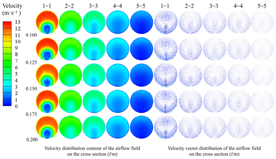
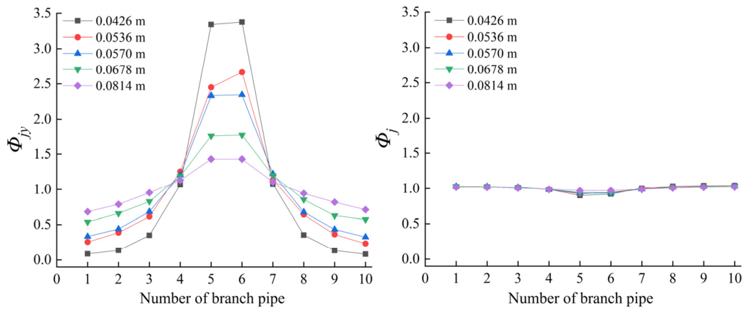
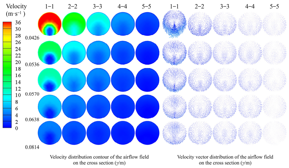
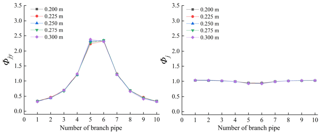
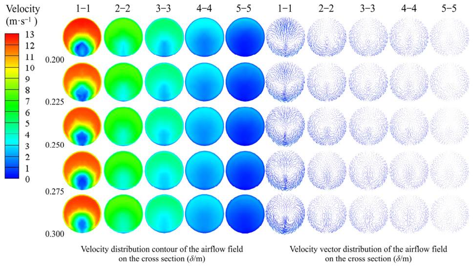
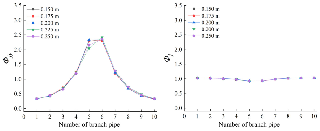
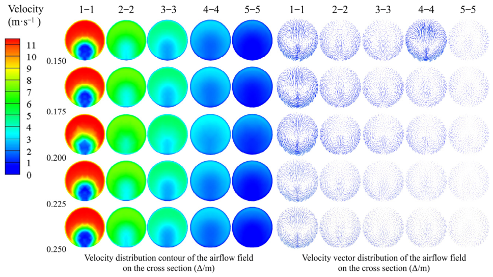
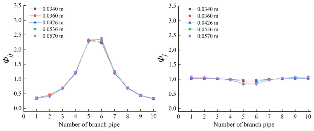
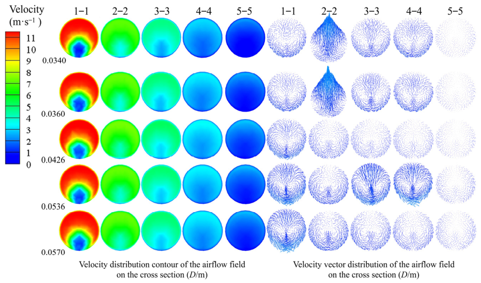
The simulation results are shown in Figure 6, Figure 7, Figure 8, Figure 9, Figure 10, Figure 11, Figure 12, Figure 13, Figure 14, Figure 15, Figure 16, Figure 17, Figure 18, Figure 19, Figure 20, Figure 21, Figure 22, Figure 23, Figure 24, Figure 25, Figure 26, Figure 27, Figure 28, Figure 29, Figure 30, Figure 31, Figure 32 and Figure 33. Figure 6, Figure 10, Figure 14, Figure 18, Figure 22, Figure 26 and Figure 30 show the variation curves of the airflow velocity along the central axis of the branch pipes under different factor levels, and Figure 7, Figure 11, Figure 15, Figure 19, Figure 23, Figure 27 and Figure 31 show the Φjy and Φj values of the airflow at the inlet and outlet boundaries of each branch pipe in the multi-branch pipeline. Figure 8, Figure 12, Figure 16, Figure 20, Figure 24, Figure 28 and Figure 32 show the variation curves of the velocity and pressure difference along the central axis of the header (the reference coordinate system is shown in Figure 2). Figure 9, Figure 13, Figure 17, Figure 21, Figure 25, Figure 29 and Figure 33 show the velocity contours at the header cross sections. On this basis, the influence of each factor on the airflow behavior of the multi-branch pipeline system was analyzed at the microscopic scale.
3.1.1. Inlet Flow Rate of Branch Pipe 1
The effect of the inlet flow rate of branch pipe 1 (Q) on the internal flow field of the pipeline system is shown in Figure 6, Figure 7, Figure 8 and Figure 9. As shown in Figure 6, the airflow velocity in each branch pipe gradually increases and then decreases rapidly along the Y axis, exhibiting an approximately symmetrical distribution about the coordinate origin O (Figure 2). Branch pipes 5 and 6, which are close to the main pipe, have higher initial airflow velocities and larger velocity reductions in the tee junction region, whereas branch pipes 1 and 10, which are farther from the main pipe, show the opposite pattern.
Figure 6.
Variation trend of axial velocity in the branch pipe—Inlet flow rate of branch pipe 1.
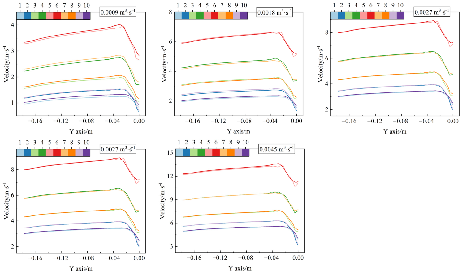
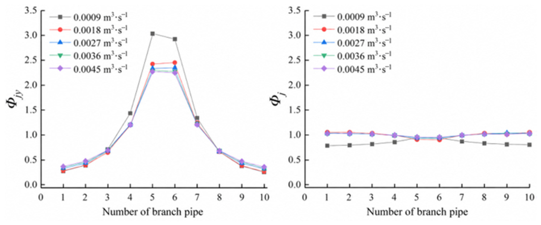
According to Equations (1) and (2) and the variations in Φjy and Φj shown in Figure 7, the static pressure difference between the branch pipes and the header generated during fan operation is the main driving force for airflow through the branch pipes. The pressure distribution within the header results in a distribution of Φjy that is higher in the middle and lower at both ends along the branch pipe sequence. As airflow travels toward the header along the Y axis, the airflow velocity in the branch pipes increases approximately linearly, indicating relatively weak flow disturbances and losses mainly attributable to frictional resistance along the branch pipes. Upon entering the tee junction region, the airflow undergoes an approximately 90° change in direction, accompanied by a sudden expansion of the flow cross section and mixing with the airflow in the header. These effects markedly increase local resistance losses, causing the airflow velocity to decrease rapidly along the Y axis. As Q increases, the airflow velocities in all branch pipes increase overall, and inertial effects become stronger, while the spatial distribution pattern determined by the pipeline geometry remains essentially unchanged. Therefore, the variation trends of Φj under different Q levels are highly consistent, in agreement with the axial momentum conservation equation in Equation (2).
Figure 7.
The Φjy and Φj values of the airflow at the inlet and outlet boundaries of each branch pipe in the multi-branch pipeline—Inlet flow rate of branch pipe 1.
The pressure and velocity variations along the header centerline reflect the cumulative effects of successive confluence at the tees. As shown in Figure 8, airflow from the branch pipes successively enters the header from both ends toward point O, progressively increasing the header flow rate and axial airflow velocity, while the pressure difference exhibits an approximately symmetrical stepwise variation. Pressure changes are relatively gradual between adjacent tees but pronounced at the tee junctions, indicating that the header pressure distribution is jointly determined by frictional resistance losses along the header and local confluence losses. As Q increases, the airflow input from the branch pipes increases, intensifying pressure variations and velocity fluctuations in the tee regions. Near the main pipe, the larger accumulated flow rate within the header strengthens the interaction between subsequent branch pipe jets and the header airflow, resulting in more pronounced local pressure gradients and velocity fluctuations.
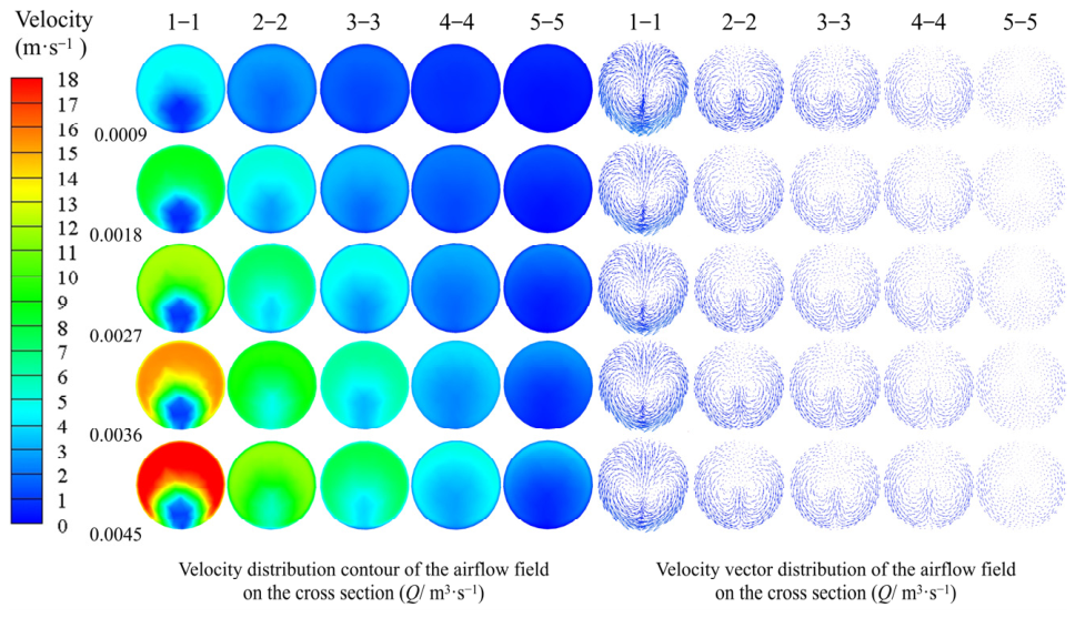
Figure 9 shows that, from cross Section 5-5 (Refer to 1-1 to 5-5 in Figure 2, and the same below), far from the main pipe, to cross Section 1-1, close to the main pipe, the average velocity and velocity gradient across the cross sections progressively increase, while the velocity distribution becomes markedly nonuniform and distinct vortices emerge. At the distant cross sections, fewer upstream branch pipes contribute to confluence, resulting in a smaller accumulated flow rate and allowing jet disturbances to decay relatively rapidly downstream. As airflow travels toward the main pipe, branch pipe jets along the Y axis successively enter the header. The limited flow development distance between adjacent branch pipes prevents the secondary flow generated by the preceding confluence from dissipating completely, causing disturbances to accumulate. Meanwhile, the increasing accumulated flow rate strengthens energy exchange between the main airflow and the incoming jets, increasing radial velocity gradients, local vortices, and energy dissipation. Therefore, confluence at successive tees exhibits pronounced cumulative effects and interactions along the flow direction, increasing flow field nonuniformity and local resistance losses near the main pipe.
Figure 8.
Variation trends of pressure gradient and velocity along the central axis of the header—Inlet flow rate of branch pipe 1.
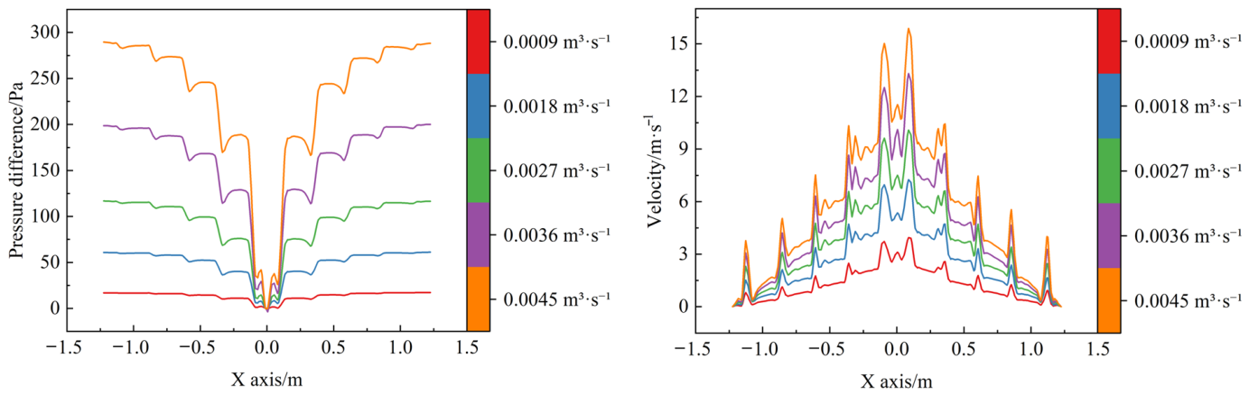
Figure 9.
Velocity contour at the header cross section—Inlet flow rate of branch pipe 1.
3.1.2. Branch Pipe Inner Diameter
The effect of the branch pipe inner diameter (d) on the internal flow field of the multi-branch pipeline system is shown in Figure 10, Figure 11, Figure 12 and Figure 13. As shown in Figure 10 and Figure 11, with increasing d, the initial airflow velocity in branch pipe 1 gradually decreases, while the distribution of Φjy changes from an approximately horizontal profile to a pattern with higher values in the middle and lower values at both ends. Branch pipes 5 and 6, close to the main pipe, exhibit the most pronounced increases in airflow velocity. At a constant Q, a smaller d increases the inlet airflow velocity and frictional resistance within the branch pipes, reducing the sensitivity of branch pipe flow rates to local pressure differences within the header and promoting a more uniform flow distribution. Conversely, increasing d reduces branch pipe resistance and strengthens the regulating effect of the header pressure distribution on branch pipe suction flow rates. The central branch pipes receive larger flow rates because of the stronger suction near the main pipe, thereby increasing velocity differences among the branch pipes (Figure 12). Upon entering the tee junction region, the axial airflow velocity in the branch pipes decreases markedly under all d conditions, with greater reductions at smaller d. This occurs because the concentrated high-velocity jets formed in smaller branch pipes undergo cross-sectional expansion and flow direction deflection upon entering the header, producing substantial local resistance losses. After confluence, Φj approaches 1 under different d conditions, indicating that the combined effects of confluence mixing and the header pressure field markedly reduce velocity differences among the branch pipe airflows after they enter the header.
Figure 10.
Variation trend of axial velocity in the branch pipe—Branch pipe inner diameter.
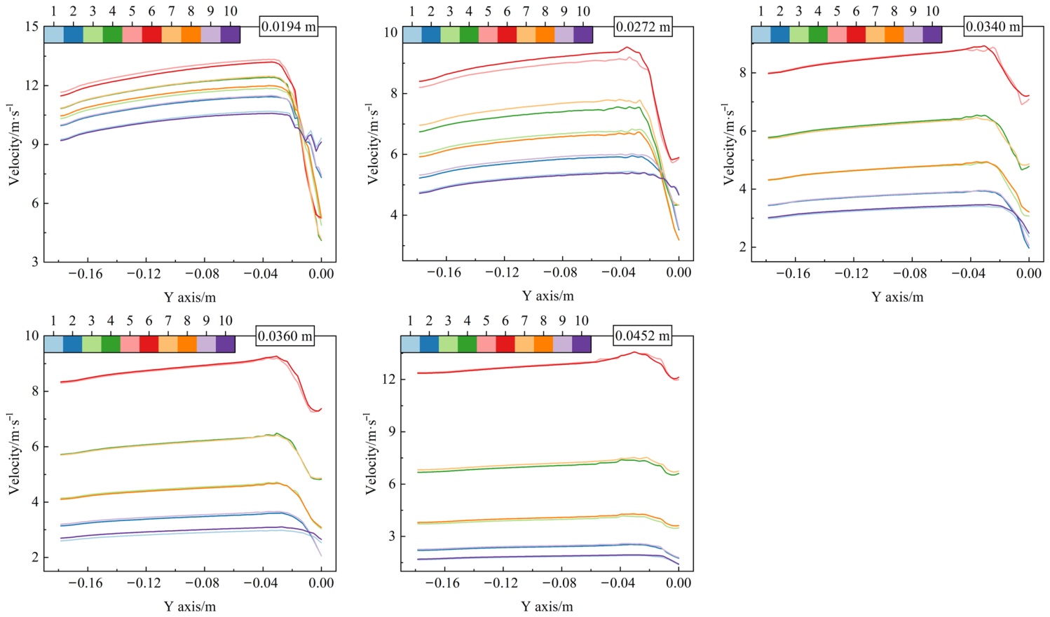
Figure 11.
The Φjy and Φj values of the airflow at the inlet and outlet boundaries of each branch pipe in the multi-branch pipeline—Branch pipe inner diameter.
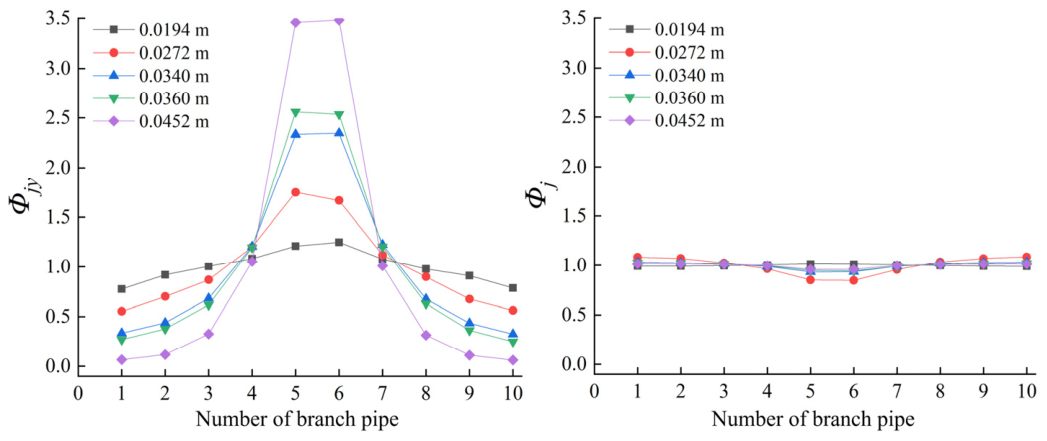
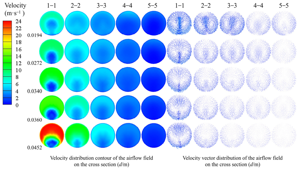
Figure 13 shows the effect of variation in d on the evolution of the flow field across the header cross sections. From cross Section 5-5, far from the main pipe, to cross Section 1-1, close to the main pipe, velocity distribution nonuniformity and vortex intensity generally increase, with cross Section 1-1 exhibiting the most pronounced velocity gradients and vortex structures. This occurs because successive inflows from the branch pipes progressively increase the header flow rate, while the limited flow development distance between adjacent branch pipes allows subsequent jets to disturb vortices generated by the preceding confluence before they fully dissipate. Therefore, under different d conditions, the continuous inflow of branch pipe jets produces a certain degree of secondary flow within the header cross sections.
Figure 12.
Variation trends of pressure gradient and velocity along the central axis of the header—Branch pipe inner diameter.
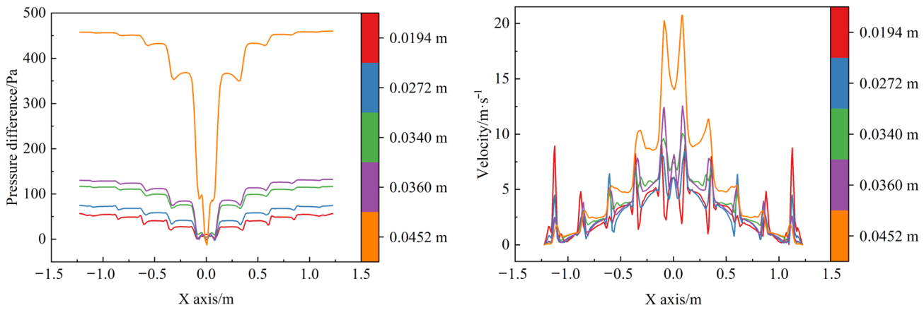
Figure 13.
Velocity contour at the header cross section—Branch pipe inner diameter.
3.1.3. Branch Pipe Length
The effect of the branch pipe length (l) on the internal flow field of the multi-branch pipeline system is shown in Figure 14, Figure 15, Figure 16 and Figure 17. As l increases, the initial airflow velocities in all branch pipes decrease slightly overall, while Φjy retains an approximately symmetrical distribution with higher values in the middle and lower values at both ends, and Φj remains close to 1. Increasing the branch pipe length increases frictional resistance along the flow path. However, because all branch pipe lengths change simultaneously, the relative effects of the header pressure field and tee geometry on flow distribution remain essentially unchanged. The airflow undergoes similar processes of flow deflection, confluence, and momentum exchange after entering the tees. Therefore, the variation patterns of Φjy and Φj remain essentially consistent under different l conditions.
As shown in Figure 16, the header pressure curves under different l conditions are clearly separated in the region far from point O but gradually converge toward point O, whereas the axial velocity distributions along the header are nearly identical. Changes in branch pipe length primarily alter frictional resistance within the branch pipes, directly affecting the flow rates entering from the distant branch pipes. As successive confluence proceeds toward the main pipe, the local header pressure becomes increasingly governed by the overall confluence state and the suction effect of the main pipe, weakening the influence of branch pipe length. Meanwhile, the pattern of axial momentum accumulation during successive confluence remains essentially unchanged, resulting in consistent axial velocity distributions along the header (Equation (2)).
Figure 17 shows that the velocity contours and vector distributions across the header cross sections are generally similar under different l conditions, with velocity and secondary flow intensity progressively increasing from cross Section 5-5 to cross Section 1-1. Because variations in l do not alter the confluence direction, tee geometry, or relative positions of the cross sections, the airflow paths after entry into the header remain essentially unchanged. Therefore, branch pipe length primarily affects frictional resistance within the straight sections of the branch pipes and has a limited influence on the overall flow field structure formed by successive confluence within the header.
Figure 14.
Variation trend of axial velocity in the branch pipe—Branch pipe length.
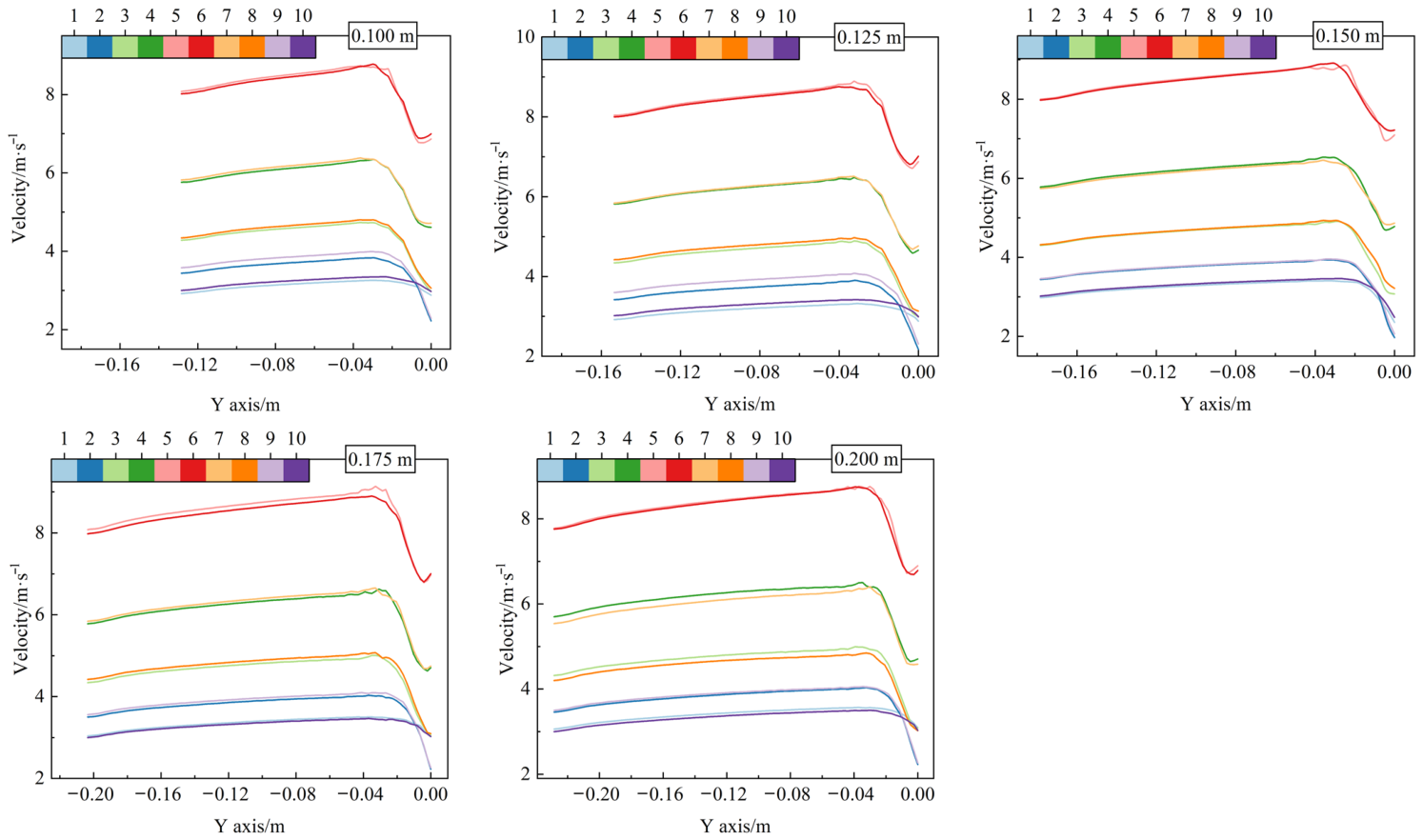
Figure 15.
The Φjy and Φj values of the airflow at the inlet and outlet boundaries of each branch pipe in the multi-branch pipeline—Branch pipe length.
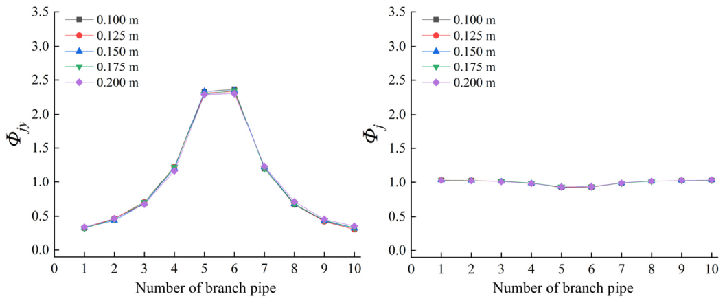
Figure 16.
Variation trends of pressure gradient and velocity along the central axis of the header— Branch pipe length.
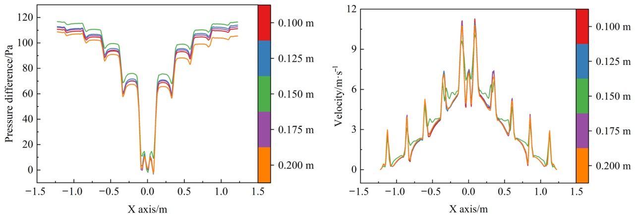
Figure 17.
Velocity contour at the header cross section—Branch pipe length.
3.1.4. Header Inner Diameter
The effect of the header inner diameter (γ) on the internal flow field of the multi-branch pipeline system is shown in Figure 18, Figure 19, Figure 20 and Figure 21. As shown in Figure 18 and Figure 19, with decreasing γ, the inlet airflow velocities of all branch pipes increase overall, and the velocity differences among branch pipes at different positions become more pronounced. Accordingly, Φjy exhibits a distinct symmetrical distribution with higher values in the middle and lower values at both ends. As γ increases, the inlet airflow velocities of the branch pipes decrease, and the Φjy curves gradually become flatter, indicating that the airflow distribution among the branch pipes tends to become more uniform. Meanwhile, under different γ conditions, Φj fluctuates only slightly around 1, indicating a high degree of consistency in the relative velocity variation after the airflow enters the tee junction region. The main reason is that, when the header inner diameter is relatively small, the cross-sectional area of the header decreases. As airflow from the branch pipes successively enters the header, the axial flow rate within the header rapidly accumulates toward the main pipe, resulting in markedly greater velocity and pressure variations in the region close to the main pipe and thereby increasing the pressure difference between the near and distant branch pipes. With increasing γ, the flow cross-sectional area of the header increases, reducing the axial velocity corresponding to the same converging flow rate and making the pressure distribution along the header more uniform. Consequently, the suction conditions experienced by branch pipes at different positions become more consistent, thereby improving the uniformity of flow distribution among the branch pipes.
Figure 18.
Variation trend of axial velocity in the branch pipe—Header inner diameter.
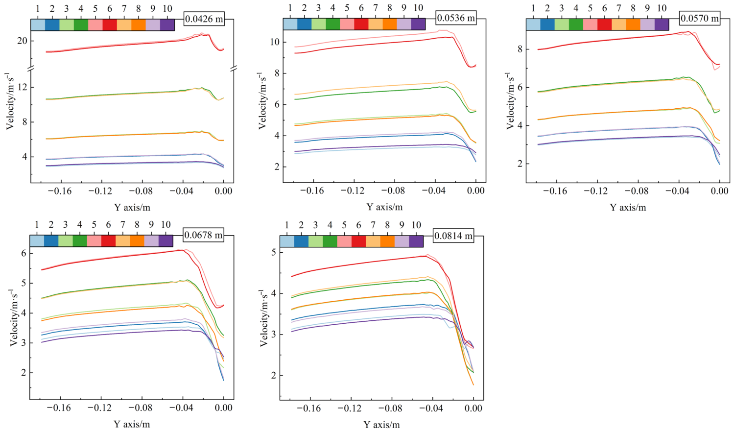
Figure 19.
The Φjy and Φj values of the airflow at the inlet and outlet boundaries of each branch pipe in the multi-branch pipeline—Header inner diameter.
As shown in Figure 20, decreasing γ markedly increases the magnitude of pressure variations along the X axis on both sides of the header. Distinct stepwise pressure changes and velocity peaks occur at the tee junctions, particularly near point O. This is because successive branch pipe inflows progressively increase the header flow rate toward the main pipe, while the smaller flow cross-sectional area increases the axial velocity and concentrates local disturbances. Increasing γ reduces the axial flow rate per unit cross-sectional area and provides more space for flow adjustment between adjacent tees, thereby reducing local velocity and pressure gradients, smoothing the curves, and narrowing the differences among junctions.
Figure 21 shows that, at smaller γ, velocity distribution nonuniformity and secondary flow intensity increase markedly from cross Section 5-5 to cross Section 1-1, where extensive high- and low-velocity regions and pronounced vortices occur. A smaller γ increases the ratio of the branch pipe inner diameter to the header inner diameter, causing the jets to occupy a larger proportion of the header cross section. Meanwhile, the nonuniform flow field generated by the preceding confluence is disturbed by subsequent jets before it fully recovers, causing velocity distortion and secondary flow to accumulate along the header. Increasing γ reduces the relative jet size and provides more space for flow development, weakening disturbance accumulation and secondary flow. Consequently, the uniformity of the velocity distribution across the header cross sections, the pressure distribution along the header, and the flow distribution among the branch pipes is improved.
Figure 20.
Variation trends of pressure gradient and velocity along the central axis of the header— Header inner diameter.
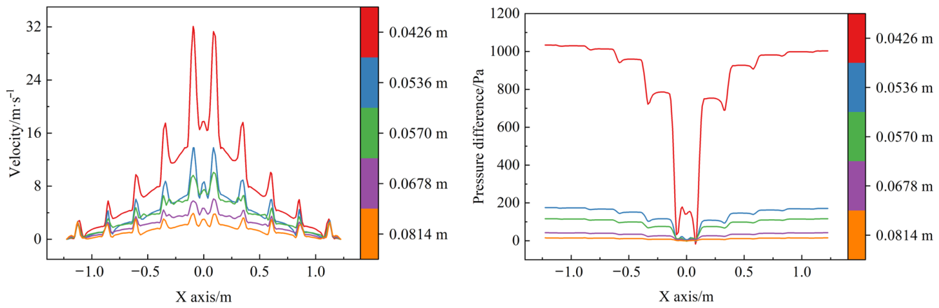
Figure 21.
Velocity contour at the header cross section—Header inner diameter.
3.1.5. Branch Pipe Spacing
The effect of the branch pipe spacing (δ) on the internal flow field of the multi-branch pipeline system is shown in Figure 22, Figure 23, Figure 24 and Figure 25. As shown in Figure 22 and Figure 23, the overall distribution patterns of the axial airflow velocity in each branch pipe and Φjy are essentially consistent, both exhibiting an approximately symmetrical pattern about point O, with higher values in the middle and lower values at both ends. As δ increases, the initial airflow velocities in the branch pipes close to the main pipe increase slightly, whereas those in the distant branch pipes change only marginally. Meanwhile, Φj fluctuates only slightly around 1 at all levels, indicating that the relative velocity distribution of the branch pipe airflow after confluence at the tees is only weakly affected by the branch pipe spacing.
Figure 22.
Variation trend of axial velocity in the branch pipe—Branch pipe spacing.
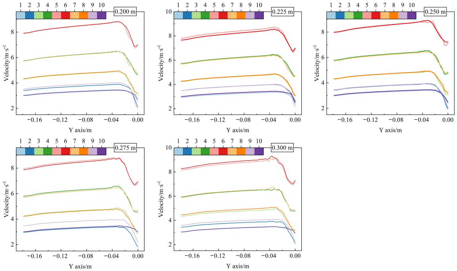
Figure 23.
The Φjy and Φj values of the airflow at the inlet and outlet boundaries of each branch pipe in the multi-branch pipeline—Branch pipe spacing.
As shown in Figure 24, the overall shapes of the pressure and velocity curves in the header are similar under different δ conditions, although the amplitudes of the local fluctuations at the tee junctions differ. When δ is relatively small, the distance between adjacent tees is shorter, and the velocity distortion and local pressure disturbance generated by the preceding confluence have not fully recovered before the airflow enters the subsequent confluence region. Consequently, flow disturbances among multiple tees are more likely to accumulate, resulting in more concentrated fluctuations in airflow pressure and velocity. As δ increases, the straight pipe sections between adjacent tees become longer, providing the airflow with a longer redevelopment distance and thereby alleviating the local disturbances to some extent.
Figure 25 shows that, under different δ conditions, velocity distribution nonuniformity and secondary flow intensity across the header cross sections generally increase from cross Section 5-5 to cross Section 1-1. Cross Section 1-1, close to the main pipe, consistently exhibits distinct high and low velocity regions and vortex structures. Increasing δ extends the flow development distance between adjacent tees, allowing the velocity distortion caused by the preceding confluence to recover partially before the airflow enters the next tee, thereby reducing the accumulation of local nonuniformity. Near the main pipe, however, the accumulated header flow rate is relatively large, and subsequent confluence still causes pronounced flow deflection, with secondary flow persisting. Therefore, branch pipe spacing primarily affects the propagation and recovery of disturbances caused by successive confluence, while the basic flow pattern of progressive convergence from both ends of the system toward the main pipe remains unchanged.
Figure 24.
Variation trends of pressure gradient and velocity along the central axis of the header—Branch pipe spacing.
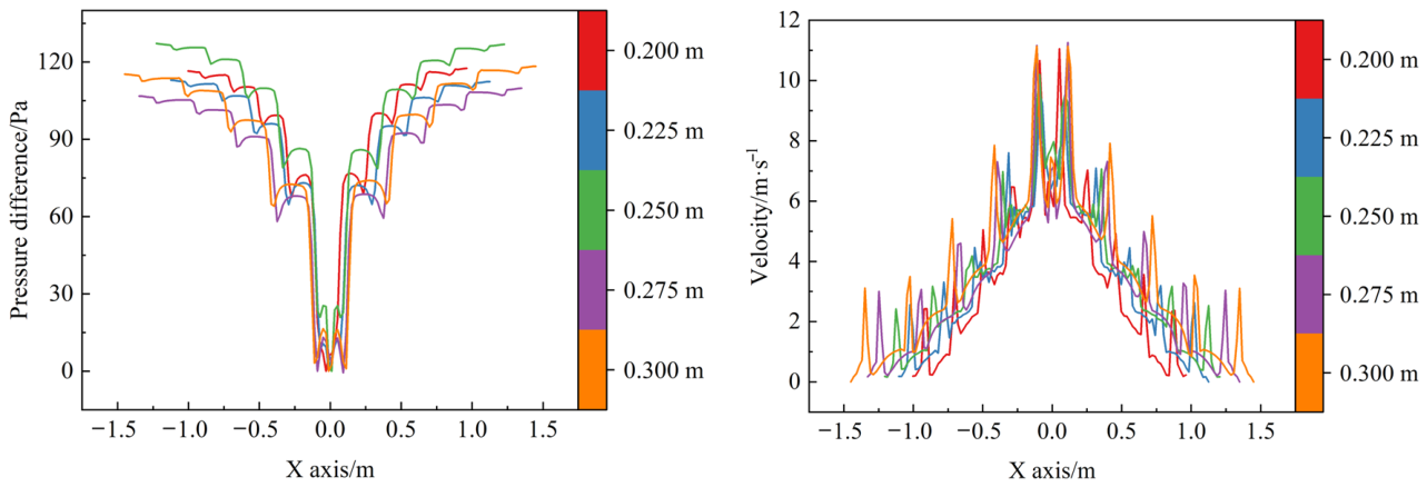
Figure 25.
Velocity contour at the header cross section—Branch pipe spacing.
3.1.6. Main Pipe Length
The effect of the main pipe length (Δ) on the internal flow field of the multi-branch pipeline system is shown in Figure 26, Figure 27, Figure 28 and Figure 29. As shown in Figure 26 and Figure 27, the overall distribution patterns of the airflow velocity along the Y axis in each branch pipe and Φjy are essentially consistent, both exhibiting an approximately symmetrical pattern about point O, with higher values in the middle and lower values at both ends. As Δ increases, the initial airflow velocities in the branch pipes close to the main pipe vary to a certain extent, whereas those in the distant branch pipes show relatively small changes. Meanwhile, Φj fluctuates only slightly around 1 at all levels, indicating that changes in the main pipe length have only a weak effect on the relative velocity distribution of the branch pipe airflow after confluence at the tees.
Figure 26.
Variation trend of axial velocity in the branch pipe—Main pipe length.
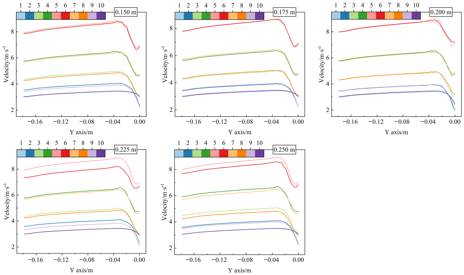
Figure 27.
The Φjy and Φj values of the airflow at the inlet and outlet boundaries of each branch pipe in the multi-branch pipeline—Main pipe length.
As shown in Figure 28, the overall shapes of the header pressure and velocity curves are relatively consistent under different Δ conditions. Increasing Δ extends the transport path of the converged airflow before it enters the fan, altering frictional resistance within the main pipe and consequently adjusting the overall pressure level in the header. However, the main pipe is located downstream of all branch pipe confluences, so changes in its length impose a common resistance condition on all branch pipes without altering the tee arrangement or progressive confluence pattern. The axial velocity variation along the header therefore remains essentially unchanged.
Figure 29 shows that the velocity distribution patterns across the header cross sections are generally consistent under different Δ conditions. Velocity nonuniformity and secondary flow intensity progressively increase from cross Section 5-5 to cross Section 1-1, whereas increasing Δ generally reduces secondary flow intensity across the cross sections. Because the main pipe length does not alter the branch pipe jet direction or tee junction angle, the high and low velocity regions and their locations remain essentially unchanged. The approximately perpendicular inflow from the branch pipes and the progressive accumulation of flow along the header sustain pronounced velocity nonuniformity and local swirling flow near the main pipe. Therefore, main pipe length has a limited influence on the header velocity distribution pattern and the relative flow distribution among the branch pipes.
Figure 28.
Variation trends of pressure gradient and velocity along the central axis of the header— Main pipe length.
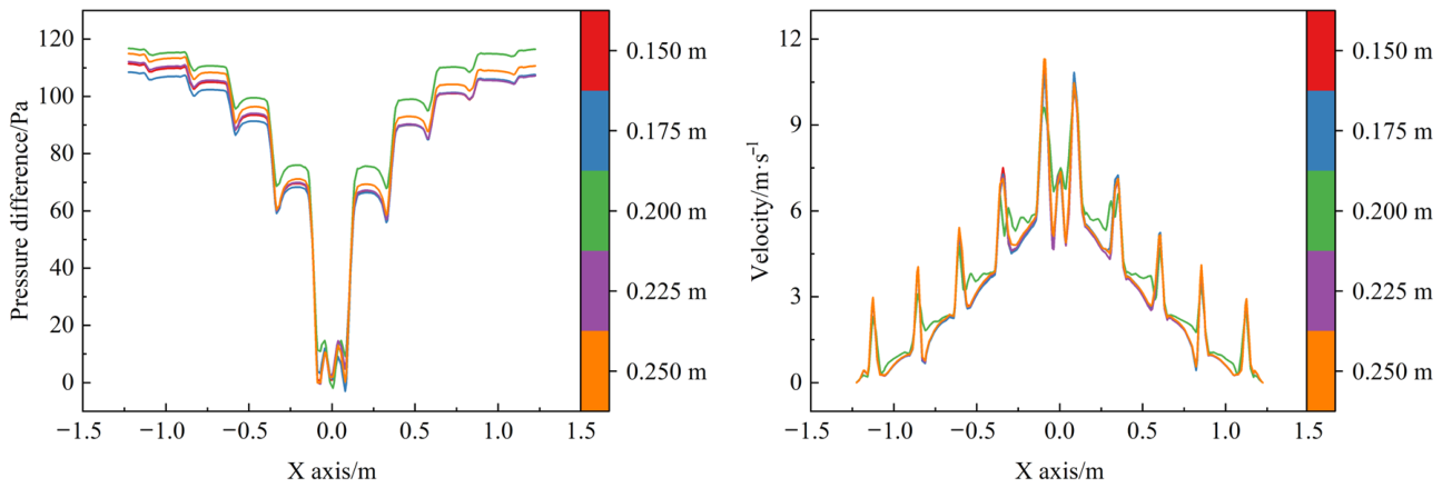
Figure 29.
Velocity contour at the header cross section—Main pipe length.
3.1.7. Main Pipe Inner Diameter
The effect of the main pipe inner diameter (D) on the internal flow field of the multi-branch pipeline system is shown in Figure 30, Figure 31, Figure 32 and Figure 33. As shown in Figure 30 and Figure 31, Φjy exhibits an approximately symmetrical distribution about point O, with higher values in the middle and lower values at both ends, under different D conditions. As D increases, the initial airflow velocities in the branch pipes show only minor changes overall, indicating that the main pipe inner diameter has a limited influence on the flow distribution pattern among the branch pipes. Under all operating conditions, Φj generally fluctuates around 1. In branch pipes 5 and 6, close to the main pipe, Φj decreases slightly with increasing D, whereas changes in the distant branch pipes are relatively small. This is because changes in D alter the flow cross-sectional area through which the converging airflow from both sides enters the main pipe, with the influence concentrated near point O. Increasing D enlarges the main pipe inlet area, causing corresponding adjustments in the velocity of the converged airflow and the local pressure distribution. Consequently, branch pipes 5 and 6, closest to the main pipe, are more strongly affected, while the influence on the distant branch pipes progressively weakens with increasing distance.
Figure 30.
Variation trend of axial velocity in the branch pipe—Main pipe inner diameter.
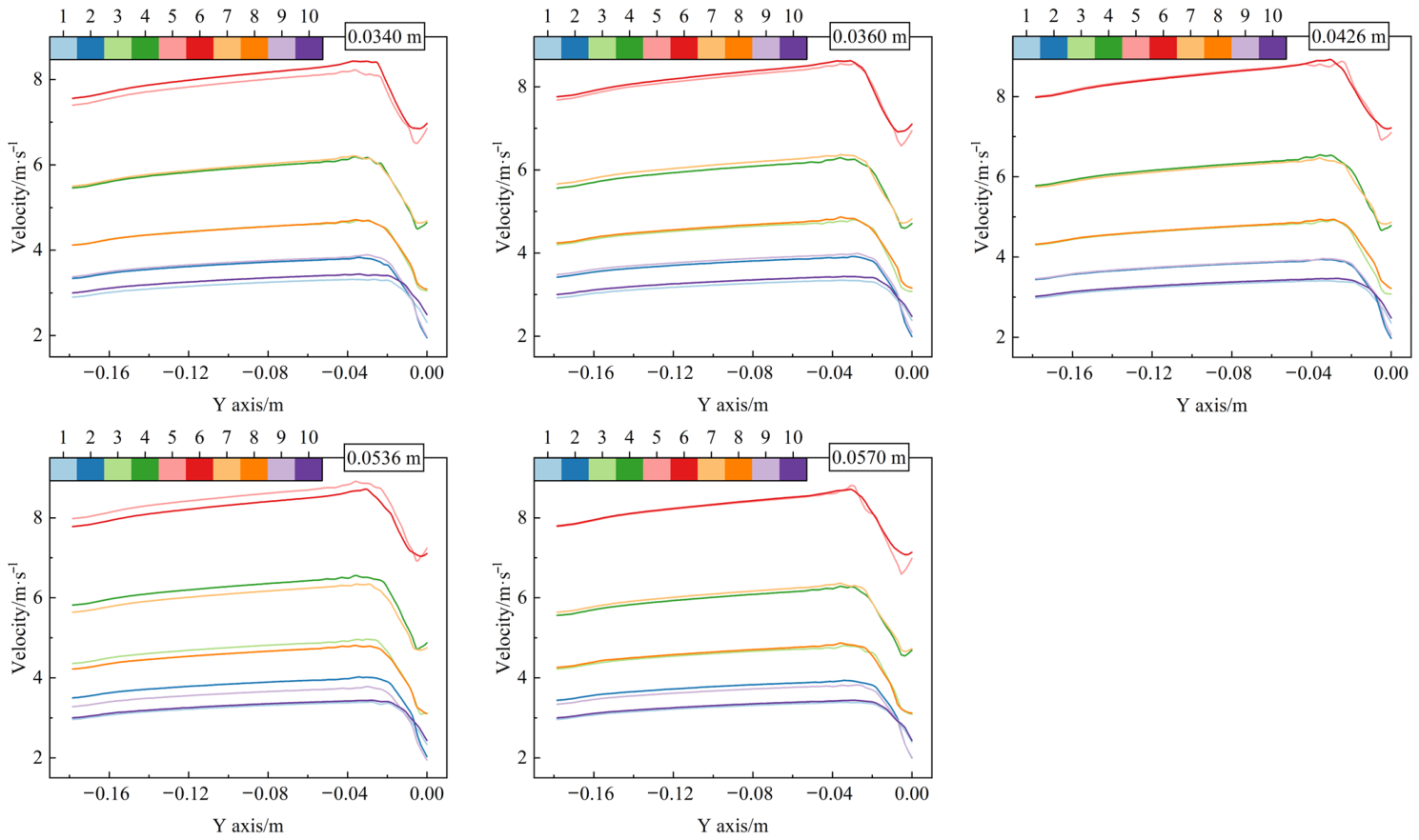
Figure 31.
The Φjy and Φj values of the airflow at the inlet and outlet boundaries of each branch pipe in the multi-branch pipeline—Main pipe inner diameter.
As shown in Figure 32, as D increases, the pressure difference along the X axis of the header decreases markedly overall. Meanwhile, similar stepwise pressure changes and local velocity peaks are still observed at the tee junctions, indicating that changes in the main pipe inner diameter do not significantly alter the velocity distribution pattern formed by successive confluence within the header. This is because the main pipe serves as the common outlet passage after the airflow from both sides of the header has progressively converged. Increasing D significantly enlarges the outlet flow cross-sectional area and reduces the flow resistance as the converged airflow enters the main pipe. Therefore, the pressure difference within the header required to maintain a similar confluence state decreases accordingly.
Figure 33 shows that, under different D conditions, velocity nonuniformity within the header generally increases progressively from cross Section 5-5 to cross Section 1-1. The flow field at cross Section 5-5 is relatively uniform, whereas the cross sections near the main pipe exhibit more distinct high- and low-velocity regions and secondary flow. This mainly results from the accumulation of flow through successive confluences along the header. The closer a cross section is to point O, the more upstream branch pipes contribute airflow and the greater the flow rate through that cross section. Meanwhile, flow deflection induced by successive tees propagates downstream, further increasing flow nonuniformity in the cross sections near the main pipe. The main pipe inner diameter primarily alters the boundary condition at point O, where the header airflow turns into the main pipe, with its influence concentrated near the main pipe. Secondary flow formation at each cross section remains primarily governed by the perpendicular junctions between the branch pipes and the header, the successive tee arrangement, and the confluence positions along the flow path. Therefore, changing D modifies the pattern and intensity of secondary flow in the cross sections near the main pipe but does not alter the overall trend of progressively increasing flow nonuniformity from cross Section 5-5 to cross Section 1-1.
Figure 32.
Variation trends of pressure gradient and velocity along the central axis of the header— Main pipe inner diameter.
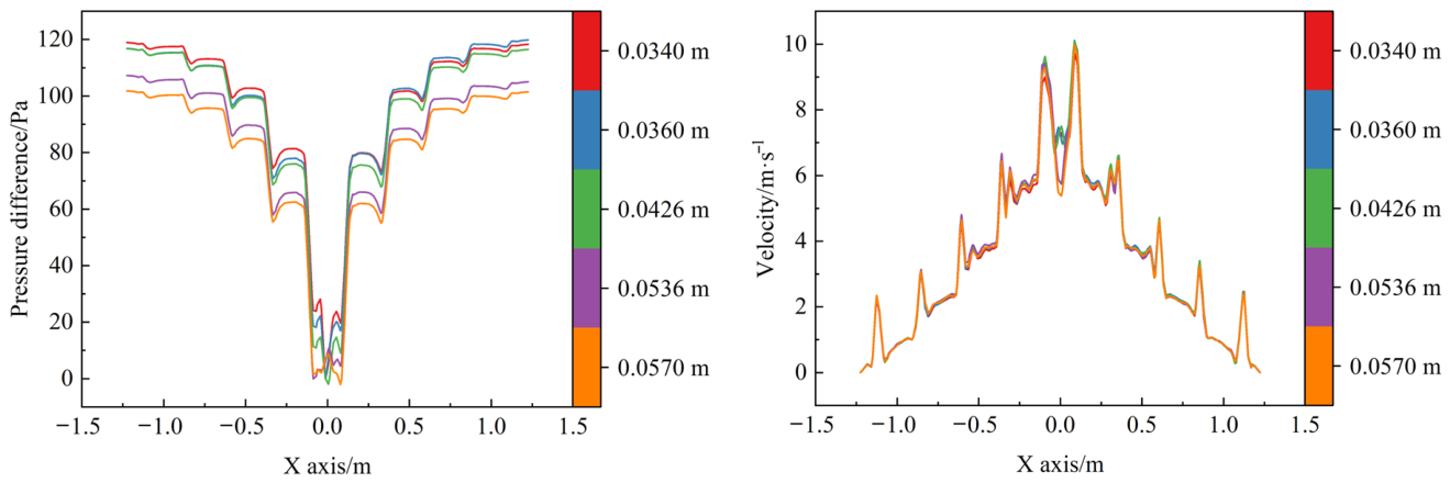
Figure 33.
Velocity contour at the header cross section—Main pipe inner diameter.
In summary, Q, d, and γ have relatively significant effects on the flow distribution among the branch pipes and on the pressure and velocity variations within the header, whereas l, δ, Δ, and D mainly alter the local flow field by regulating local resistance or downstream flow conditions. Overall, the flow rate in each branch pipe is constrained by the pressure distribution within the header, exhibiting an approximately symmetrical distribution along the branch pipe sequence, with higher values in the region close to the main pipe and lower values at the distant ends. After the fan begins operating, as airflow from the branch pipes successively enters the header, the flow rate within the header progressively accumulates toward the main pipe. The closer the flow is to the main pipe, the more pronounced the flow field nonuniformity and the cumulative coupling effect of successive confluence become. Therefore, relying solely on microscopic flow field parameters, such as local pressure and velocity within the branch pipes or header, makes it difficult to establish a direct and unified quantitative relationship between the pipeline structure and the main pipe flow demand. Accordingly, it is necessary to investigate the system from a macroscopic perspective and establish a relationship model incorporating the above experimental factors and the main pipe flow rate, thereby enabling accurate prediction of the main pipe flow demand under different pipeline structures and operating conditions and providing a theoretical basis for subsequent fan capacity matching and selection.
3.2. Bench Test Results and Analysis
3.2.1. Fitting of Bench Test Results to the Π Equation
Table 5 presents the bench test results for the component relationships between Π1 and each of the dimensionless parameters Π2 to Π8. The fourth-order polynomial fits described in Section 2.4.3 yielded a coefficient of determination of R2 = 0.99. The fitted coefficient vectors A2 to A8 are given in Equation (10).
Table 5.
Bench test results.
At the common reference condition, the value of Π1 obtained from the bench test data in Table 5 was 176,453.804, as given in Equation (11).
Combined with Equation (5), substituting the physical quantities contained in the Π1 term into Equations (9) and (11) yields:
Furthermore, the empirical formula for quantitatively predicting the main pipe flow rate was obtained as follows:
where q is the main pipe flow rate, and the Πi terms corresponding to each component equation are detailed in Table 5.
3.2.2. Validation of the Main Pipe Flow Demand Prediction Model
The validation results are presented in three stages, following the procedure described in Section 2.4.3.
(1) Prediction accuracy of the empirical formula for main pipe flow rate
The experimental factors and their corresponding test point parameters were converted into the respective dimensionless parameters Π2–Π8 and substituted separately into Equation (13) to obtain the corresponding predicted q values. The results calculated using Equation (13) were compared with the measured main pipe flow rates, as shown in Figure 10. As shown in Table 6, the absolute values of the relative errors between the predicted and measured main pipe flow rates at all test points were less than 0.5%, indicating that the established empirical model has high prediction accuracy within the range of the modeling test points.
Table 6.
Results of the first validation test.
(2) Validation of component equation validity and applicable parameter range
To further verify the validity of each component equation under different fixed test conditions, the component equations corresponding to Π2–Π8 in Equation (13) were examined separately. When validating a given dimensionless component Πi, the remaining test factors were kept unchanged, and tests were conducted again using fixed test values different from those adopted when establishing the corresponding component fitting equation. First, under the two sets of fixed test conditions, the remaining dimensionless parameters other than the component to be validated were substituted into their respective component equations, and the corresponding common product terms were calculated according to the product combination relationship in Equation (9), thereby obtaining the normalized reference terms corresponding to the component to be validated under different fixed conditions. Subsequently, the Πi values obtained from the validation tests were substituted into the corresponding component fitting equation, and the normalized component values under the two fixed test conditions were calculated separately, followed by a comparison of their relative deviations.
In the above equation, according to Equation (8) and Table 5, the following can be obtained:
where i = 2, 3, 4, 5, 6, 7, and 8; ai are given by the following determinants:
Following the above method, Π2, Π3, Π4, , , , , , and were sequentially substituted into Equation (14) for validation, and the results are presented in Table 7. The results of the second validation indicate that when 571.79 ≤ Π2 ≤ 2858.97, 0.194 ≤ Π3 ≤ 0.452, 1 ≤ Π4 ≤ 2, 2 ≤ Π5 ≤ 3, 0.426 ≤ Π6 ≤ 0.814, 1.5 ≤ Π7 ≤ 2.5, and 0.34 ≤ Π8 ≤ 0.57, the relative deviation of the equation is less than 10%, satisfying the requirements of general engineering applications.
Table 7.
Results of the second validation test.
(3) Validation of component equation validity and applicable parameter range
To further verify the reliability of the parameter range determined by the second validity test, several independent combinations of structural parameters and operating conditions, different from the test points used for model development and the second validation, were selected for additional validation tests. The corresponding Q, d, l, δ, γ, Δ, and D for each independent validation condition were converted into the respective dimensionless parameters and substituted into Equation (10). Equation (13) was then used to calculate the predicted main pipe flow rate, which was compared with the actual main pipe flow rate measured in the bench test. The results are presented in Table 8.
Table 8.
Results of the third validation test.
Based on the results of the second and third validity tests, it was finally determined that when the parameters were within the ranges of 571.79 ≤ Π2 ≤ 2858.97, 0.194 ≤ Π3 ≤ 0.452, 1 ≤ Π4 ≤ 2, 2 ≤ Π5 ≤ 3, 0.426 ≤ Π6 ≤ 0.814, 1.5 ≤ Π7 ≤ 2.5, and 0.34 ≤ Π8 ≤ 0.57, the relative error between the main pipe flow rate predicted by Equation (13) and the measured value was less than 10%. This indicates that the established empirical formula can be used for the quantitative prediction of main pipe flow demand under different multi-branch pipeline structures and operating conditions.
Based on the results of the three validity tests and Equation (5), the final applicable parameter range of Equation (13) was determined as 0.0009 m3·s−1 ≤ Q ≤ 0.0045 m3·s−1, 0.0194 m ≤ d ≤ 0.0452 m, 0.1 m ≤ l ≤ 0.2 m, 0.2 m ≤ δ ≤ 0.3 m, 0.0426 m ≤ γ ≤ 0.0814 m, 0.15 m ≤ Δ ≤ 0.25 m, and 0.034 m ≤ D ≤ 0.057 m. This parameter range covers existing specialized seeders for crops such as rice, maize, and rapeseed [20,34,38]. Within this range, the relative error between the predicted and measured main pipe flow rates can be controlled within ±10%, indicating that the model can accurately predict the main pipe flow demand under different pipeline structures and operating conditions and can provide a quantitative basis for subsequent fan flow capacity matching and selection.
Based on the results of the three validity tests of Equation (13), further simplification yields the following empirical formula for quantitative prediction of the main pipe flow rate in the multi-branch pipeline system:
where ξ ∈ (Q d l δ γ Δ D). When ξ is the set element Q, k is the product of the functions corresponding to the remaining geometric elements in the set, with the values of these geometric elements taken as the initial dimensions of the pipeline; in this case, the recommended value of k ranges from 0.99 to 1. When ξ is any geometric element in the set other than Q, k is the product of the functions corresponding to the remaining elements in the set, with the values of these geometric elements taken as the initial dimensions of the pipeline; in this case, k can be determined as 21,969.584–21,987.452 based on the actual test results.
4. Discussion
This study addressed the difficulty of accurately determining the main pipe flow demand in a multi-branch pipeline operating under negative pressure in an air-suction seeder by examining successive confluence, changes in the local flow field, and the overall flow response of the system. The simulation results showed that the inlet flow rate of branch pipe 1, the branch pipe inner diameter, and the header inner diameter had more pronounced effects on the pressure and velocity distributions within the header. The branch pipe length, branch pipe spacing, main pipe length, and main pipe inner diameter mainly affected the local flow field by altering flow resistance, the distance available for flow development, or downstream flow conditions. As airflow from successive branch pipes entered the header, the flow rate in the header progressively increased toward the main pipe. Velocity distortion and pressure disturbances generated at adjacent tees affected the downstream flow field, leading to greater velocity nonuniformity and more pronounced secondary flow near the main pipe. Under steady-state conditions with negligible density variation and no leakage, the main pipe flow rate equals the sum of the actual branch pipe flow rates. Because the flow rate of a seed metering device operating independently may differ from its flow rate when connected to the header, estimates of main pipe flow demand need to account for the actual operating conditions of the branch pipes in the confluence system.
Previous studies have informed the design of pneumatic systems for seeders by examining pipeline resistance, airflow distribution, and operating parameters. In ref. [25], a model was developed to predict the overall pressure loss in a multi-branch confluence pipeline. The prediction error was below 10% within the reported range of applicability, and the applicable main pipe inner diameters fell within two separate intervals. For the fixed layout with 10 branch pipes examined in this study, the proposed model covers a wider range of branch pipe inner diameters and a single continuous interval of main pipe inner diameters. The study in [35] mainly investigated the total inlet flow rate, the inner diameter of the outlet branch pipes, the length of the closed end section of the header, and the positions of the outlet branch pipes. Under the reported conditions, the relative deviations in predicted velocities for outlet branch pipes 1, 2, and 3 were below 10%. The present study also considered the branch pipe length, the header inner diameter, and the length and inner diameter of the main pipe, allowing the effects of geometric parameters at different locations in the pipeline on the main pipe flow rate to be examined. The study in [38] optimized the air distributor structure and the geometry of the connecting section in a positive pressure precision maize seeder. Comparative tests showed that the optimized air distribution device reduced the pressure loss from over 30% with a conventional design to less than 10%, with a coefficient of variation in pressure across the seeding rows of less than 4%. That study aimed to reduce pressure loss and improve the uniformity of air delivery across seeding rows, whereas the present study quantifies the relationship between pipeline geometry, the inlet flow rate of branch pipe 1, and the main pipe flow rate under negative pressure confluence conditions. The study in [20] primarily examined the seed metering disc speed, the number of seed metering devices, and the rated power and operating speed of the fan. The relative errors obtained in validation ranged from −8.23% to 6.62% for the fan selection model and from −6.12% to 8.25% for the negative pressure prediction model. The study in [39] established a relationship between the total flow rate on the negative pressure side, the fan speed, and the size of the air vent on the positive pressure side. These two studies focused on operating parameters and the dimensions of specific components. The present study considered a broader set of geometric parameters for the branch pipes, header, and main pipe and incorporated six geometric parameters and the inlet flow rate of branch pipe 1 into a single empirical equation. Compared with conventional calculations for multi-branch pipelines, the calibrated equation provides a direct estimate of the main pipe flow rate from these inputs without solving for the flow rate and pressure loss in each branch under each operating condition. The predicted main pipe flow rate provides reference data for fan selection, which also requires the system pressure demand at the target flow rate and the pressure–flow characteristics of candidate fans.
The model was calibrated and tested under steady-state bench conditions for a fixed layout with 10 branch pipes. The ranges of the dimensionless parameters examined for this layout were 571.79 ≤ Π2 ≤ 2858.97, 0.194 ≤ Π3 ≤ 0.452, 1 ≤ Π4 ≤ 2, 2 ≤ Π5 ≤ 3, 0.426 ≤ Π6 ≤ 0.814, 1.5 ≤ Π7 ≤ 2.5, and 0.34 ≤ Π8 ≤ 0.57 (i.e., 0.0009 m3·s−1 ≤ Q ≤ 0.0045 m3·s−1, 0.0194 m ≤ d ≤ 0.0452 m, 0.1 m ≤ l ≤ 0.2 m, 0.2 m ≤ δ ≤ 0.3 m, 0.0426 m ≤ γ ≤ 0.0814 m, 0.15 m ≤ Δ ≤ 0.25 m, and 0.034 m ≤ D ≤ 0.057 m). The relative errors at the original calibration points were below 0.5%, and the absolute relative prediction errors for the five additional bench test conditions ranged from 0.9% to 3.2%. Because each additional condition differed from the baseline in only one factor, this error range describes the prediction performance under those tested conditions. For systems with the same branch count and layout and with parameters within the investigated ranges, the existing equation can be used for preliminary estimates without repeating CFD simulations for each condition. Additional bench tests are needed to quantify prediction errors when several factors vary simultaneously. Changes in the number or arrangement of branch pipes require separate evaluation. For a new layout, CFD can be used to examine changes in the flow field, and predictions from the original equation can be compared with bench measurements for the new layout before recalibration to quantify extrapolation errors. The effects of field disturbances, such as fluctuations in fan speed, hose deformation, and machine vibration, on model performance remain to be verified.
5. Conclusions
This study addressed the prediction of main pipe flow rate in a multi-branch confluence pipeline operating under negative pressure in an air-suction precision hill-drop rice seeder. The effects of pipeline geometry and the inlet flow rate of branch pipe 1 on airflow confluence were examined. An empirical model was developed for a fixed layout with 10 branch pipes, and its prediction accuracy was evaluated through full-scale bench tests. The main conclusions are as follows.
(1) Under the conditions examined, the inlet flow rate of branch pipe 1, the branch pipe inner diameter, and the header inner diameter had more pronounced effects on the pressure and velocity distributions within the header. The branch pipe length, branch pipe spacing, main pipe length, and main pipe inner diameter mainly affected the local flow field by altering flow resistance, the distance available for flow development, or downstream flow conditions. As airflow from successive branch pipes entered the header, the flow rate progressively increased toward the main pipe. Velocity distortion and pressure disturbances generated at adjacent tees affected the downstream flow field, resulting in greater velocity nonuniformity and more pronounced secondary flow near the main pipe.
(2) The empirical model developed using dimensional analysis directly estimates the main pipe flow rate from the inlet flow rate of branch pipe 1 and six geometric parameters of the pipeline. The parameter ranges were 0.0009 m3·s−1 ≤ Q ≤ 0.0045 m3·s−1, 0.0194 m ≤ d ≤ 0.0452 m, 0.1 m ≤ l ≤ 0.2 m, 0.2 m ≤ δ ≤ 0.3 m, 0.0426 m ≤ γ ≤ 0.0814 m, 0.15 m ≤ Δ ≤ 0.25 m, and 0.034 m ≤ D ≤ 0.057 m. Across the three validation stages, the relative errors in the predicted main pipe flow rate were within ±10% under the conditions tested. For the fixed layout with 10 branch pipes, the absolute relative prediction errors ranged from 0.9% to 3.2% across five steady-state bench test conditions excluded from model fitting, each differing from the baseline in only one factor. The predicted flow rates provide reference data for pipeline design and fan flow capacity matching for this layout. Further validation is required to assess prediction accuracy when multiple factors vary simultaneously or when the number or arrangement of branch pipes changes.
Author Contributions
Conceptualization, W.Q. and Y.Z.; methodology, J.W.; software, J.W.; validation, X.D., J.F., and W.Y.; formal analysis, K.W.; investigation, S.H.; resources, Y.Z.; data curation, Z.H.; writing—original draft preparation, J.W.; writing—review and editing, W.Q., J.W., and Y.Z.; project administration, Y.Z.; funding acquisition, W.Q. and Y.Z. All authors have read and agreed to the published version of the manuscript.
Funding
This research was funded by Opening Fund of State Key Laboratory of Agricultural Equipment Technology, grant number SKL-2025-003, and the Key Area Research and Development Program of Guangdong, grant number 2023B0202130001.
Data Availability Statement
Data are contained within the article.
Conflicts of Interest
The authors declare no conflicts of interest.
References
- Xing, H.; Cao, X.; Zhong, P.; Wan, Y.; Lin, J.; Zang, Y.; Zhang, G. DEM-CFD coupling simulation and optimisation of rice seed particles seeding a hill in double cavity pneumatic seed metering device. Comput. Electron. Agric. 2024, 224, 109075. [Google Scholar] [CrossRef] [Scilit]
- Wang, Z.; Chen, Y.; Adilet, S.; Wei, N.; Zhou, J.; Zhang, D.; Jiang, Y.; Fan, Y.; Zhang, W.; Chen, J. Design and Optimization of a Combined Seed Cleaning Mechanism for an Air-Suction Seed Metering Device for Small-Seed Crops with Multi-Seed Hill. Sustainability 2026, 18, 4274. [Google Scholar] [CrossRef] [Scilit]
- Wang, W.; Song, L.; An, X.; Quan, L.; Xie, D.; Chen, Y.; Li, Z.; Wu, Z.; Chen, L. Optimizing seed filling performance of the double-filling air suction maize and soybean seed metering device based on DEM-CFD coupling method. Comput. Electron. Agric. 2025, 237, 110586. [Google Scholar] [CrossRef] [Scilit]
- Zhao, P.; Song, Q.; Bi, Y.; Dong, J.; Fu, Z.; Huang, Y.; Zheng, Y. Interaction mechanisms of seed suction and cleaning negative pressure of an air-suction seed metering device for maize breeding plots. Biosyst. Eng. 2026, 262, 104368. [Google Scholar] [CrossRef] [Scilit]
- Huang, Z.; Jiang, Y.; Qin, W.; He, S.; Qian, C.; Wang, Z.; Zang, Y. Establishment and validation of a negative pressure prediction model for rice air-suction seed-metering device. Biosyst. Eng. 2025, 253, 104126. [Google Scholar] [CrossRef] [Scilit]
- He, K.; Chen, J.; Pan, F.; Wang, B.; Ji, C. Adaptive negative-pressure control system for electric-driven seeding blowers based on a DILPSO-fuzzy PID controller. Comput. Electron. Agric. 2025, 239, 110833. [Google Scholar] [CrossRef] [Scilit]
- Li, Z.; Ren, D.; Huang, J.; Wu, J.; Duan, D.; Zhang, T.; Chen, Y. Analysis of the seed filling performance influenced by maize seed shape, posture, and suction force. Biosyst. Eng. 2025, 256, 104186. [Google Scholar] [CrossRef] [Scilit]
- Li, B.; Wang, X.; Liu, Z.; Li, Y.; Liu, P.; Yang, F.; Liu, J. Multi-algorithm fusion based control strategy for electrically-driven wind pressure regulation in pneumatic precision seeders. Comput. Electron. Agric. 2026, 240, 111173. [Google Scholar] [CrossRef] [Scilit]
- MONOSEM. MONOSEM Check NG Plus/ NG PLUS E. Available online: https://www.monosem.com/precision-planters/single-seed-planter/pneumatic-planter/ng-plus-ng-plus-e/ (accessed on 29 September 2026).
- Kverneland Group. Optima R. Available online: https://ien.kverneland.com/seeders/pneumatic-precision-drills/optima-r (accessed on 29 September 2026).
- MASCHIO GASPARDO Group. Mounted Pneumatic Precision Planter with Fixed Frame. Available online: https://www.maschiogaspardo.com/en_row/mtr.html (accessed on 29 September 2026).
- Li, Z.; Zhang, H.; Xie, R.; Gu, X.; Du, J.; Chen, Y. Evaluation on the performance of airflow distribution device of pneumatic seeder for rapeseed through CFD simulations. Agriculture 2022, 12, 1781. [Google Scholar] [CrossRef] [Scilit]
- Zhang, W.; Li, A.; Gao, R.; Yang, C.; Gao, X.; Du, F. Flow performance evaluation and structural optimization of the dividing manifold systems using multi-attribute decision analysis. J. Build. Eng. 2024, 85, 108652. [Google Scholar] [CrossRef] [Scilit]
- Minocha, N.; Joshi, J.B. 3D CFD simulation of turbulent flow distribution and pressure drop in a dividing manifold system using OpenFOAM. Int. J. Heat Mass Transf. 2020, 151, 119420. [Google Scholar] [CrossRef] [Scilit]
- Kodali, C.; Idem, S. Modeling Flow and Pressure Distributions in Multi-Branch Light-Commercial Duct Systems. Sci. Technol. Built Environ. 2021, 27, 240–252. [Google Scholar] [CrossRef] [Scilit]
- Kogekar, G.; Kee, R.J. Model-Based Performance for Gas Distribution from Perforated Manifolds and Spargers. Chem. Eng. Process. Process Intensif. 2019, 140, 127–135. [Google Scholar] [CrossRef] [Scilit]
- Wu, P.; Cai, Z. Flow Field Characteristics and Multi-Objective Optimization of a Rectangular Gas Distributor. Proc. Inst. Mech. Eng. Part E J. Process Mech. Eng. 2026. onlinefirst. [Google Scholar] [CrossRef] [Scilit]
- Mayanja, I.K.; Donis-González, I.R. Design and Optimization of an Air Distributor for an Almond Stockpile Heated and Ambient Air Dryer (SHAD)-Part 1. Biosyst. Eng. 2023, 235, 180–188. [Google Scholar] [CrossRef] [Scilit]
- Zhang, W.; Deng, X.; Li, A.; Du, F.; Yang, C.; Gao, R.; Yin, H.; Zhang, Z. Flow Characteristics and Structural Optimization of Uniform Air Supply Duct Systems in Subway Stations for Improving Airflow Uniformity. Build. Environ. 2026, 288, 114003. [Google Scholar] [CrossRef] [Scilit]
- Shu, C.; Wei, Y.; Liao, Y.; Lei, X.; Li, Z.; Wang, D.; Liao, Q. Influence of air blower parameters of pneumatic seed-metering system for rapeseed on negative pressure characteristics and air blower selection. Trans. Chin. Soc. Agric. Eng. 2016, 32, 26–33. [Google Scholar]
- Wang, Y.; Su, W.; Lai, Q.; Lin, Y.; Gao, X. Simulation and measurement of the suction force on ellipsoidal seeds in an air-suction seed-metering device. Biosyst. Eng. 2023, 232, 97–113. [Google Scholar] [CrossRef] [Scilit]
- Wang, Z.; Su, W.; Lai, Q.; Li, J.; Gao, X. Boundary modelling of the effective suction domain of an air-suction seed-metering device for quasi-spherical seeds. Biosyst. Eng. 2024, 238, 212–226. [Google Scholar] [CrossRef] [Scilit]
- Zha, X.; Chen, L.; Chen, D.; He, Y.; Yang, R. Design and testing of a branched air-chamber type pneumatic seed metering device for rice. Agriculture 2024, 14, 1934. [Google Scholar] [CrossRef] [Scilit]
- Gao, G. Dimensional Analysis: Theories and Applications; Science Press: Beijing, China, 2021. [Google Scholar]
- Qin, W.; Wang, Z.; Wang, Y.; Qian, C.; He, S.; Zhang, M.; Zang, Y. Analysis and experiments of the air pressure loss in multi-branch convergence pipe of air suction seeder. Trans. Chin. Soc. Agric. Eng. 2023, 39, 1–14. [Google Scholar]
- Sawada, Y.; Ito, S.; Endo, I.; Hanai, H.; Horibe, K. Development of pneumatic direct seeding system for submerged paddy field (Part 1)—Basic study on the development of seeding system. J. Jpn. Soc. Agric. Mach. 1996, 58, 69–76. [Google Scholar]
- Li, J.; Lai, Q.; Su, W.; Xie, Y.; Zhang, Z. Research on the influence of the suction force on spherical particles in suction flow. Powder Technol. 2021, 393, 824–836. [Google Scholar] [CrossRef] [Scilit]
- Ghasemi, J.; Moradi, M.; Karparvarfard, S.H.; Golmakani, M.T.; Mousavi Khaneghah, A. Thin layer drying kinetics of lemon verbena leaves: A quality assessment and mathematical modeling. Qual. Assur. Saf. Crops Foods 2021, 13, 59–72. [Google Scholar] [CrossRef] [Scilit]
- Ogunnigbo, C.O.; Adetan, D.A.; Morakinyo, T.A. A study on the mathematical model for predicting the peel removal efficiency of a cassava peeler. Res. Agric. Eng. 2022, 68, 18–26. [Google Scholar] [CrossRef] [Scilit]
- Tupkar, A.; Suhane, R. Establishment of mathematical model to predict the dehulling efficiency in miniature pulse splitter machine energized by human powered flywheel motor using dimensional analysis. Mater. Today Proc. 2022, 65, 3567–3572. [Google Scholar] [CrossRef] [Scilit]
- Zare, D.; Nourmohamadi-Moghadami, A.; Panigrahi, S.S.; Karim, A.; Singh, C.B. Dimensionless modeling of fine material distribution in an experimental silo during central spout loading. J. Stored Prod. Res. 2023, 100, 102063. [Google Scholar] [CrossRef] [Scilit]
- Chen, J.; Hu, W.; Dong, X.; Lin, J.; Gao, Z.; Qiu, B. Prediction of droplet size and spreading parameter by rotary cup atomisation using dimensional analysis. Biosyst. Eng. 2025, 253, 104132. [Google Scholar] [CrossRef] [Scilit]
- Labad, R.; Mohammedi, Z.; Tayeb, R.H.; Taibi, S.; Shinde, G.U.; Feddal, M.A. Dimensional analysis based prediction model for fuel consumption in the Deutz Agrotrac tractor. Agric. Sci. Dig. 2026, 46, 383–389. [Google Scholar]
- Qin, W.; Wang, Z.; Zhang, M.; He, S.; Wang, X.; Jiang, Y.; Huang, Z.; Zang, Y. Airflow distribution law of multi-branch pipe of pneumatic rice direct seeder based on dimensional analysis. Int. J. Agric. Biol. Eng. 2023, 16, 111–127. [Google Scholar] [CrossRef] [Scilit]
- Xing, H.; Wang, Z.; Luo, X.; Zang, Y.; He, S.; Xu, P.; Liu, S. Design and experimental analysis of rice pneumatic seeder with adjustable seeding rate. Int. J. Agric. Biol. Eng. 2021, 14, 113–122. [Google Scholar] [CrossRef] [Scilit]
- Song, P.; Yang, L. Research and design on flow characteristics of single-phase multi-branch parallel pipeline. Pet. Refin. Eng. 2020, 50, 42–47. [Google Scholar]
- Qin, L.; Zhou, F.; Yang, J.; Wu, R.; Lu, L. Numerical Research on Flow Distribution and Pressure Loss of Multi-Branch Pipeline Based on Confluence and Distribution. J. South China Univ. Technol. (Nat. Sci. Ed.) 2021, 49, 109–119. [Google Scholar]
- Yin, X.; Yang, L.; Zhang, D.; Cui, T.; Han, D.; Zhang, T.; Yu, Y. Design and experiment of balance and low-loss air allotter in air pressure maize precision planter. Trans. Chin. Soc. Agric. Eng. 2016, 32, 9–17. [Google Scholar]
- Liao, Q.; Yang, S.; Liao, Y.; Cong, J.; Wang, L. Modeling for performance and parameters of pneumatic seed-metering of precision planter for rapeseed. Trans. Chin. Soc. Agric. Eng. 2013, 29, 9–15. [Google Scholar]
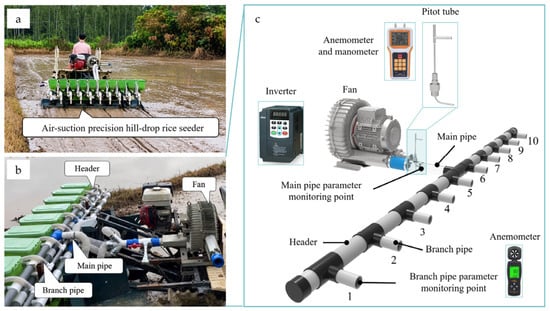
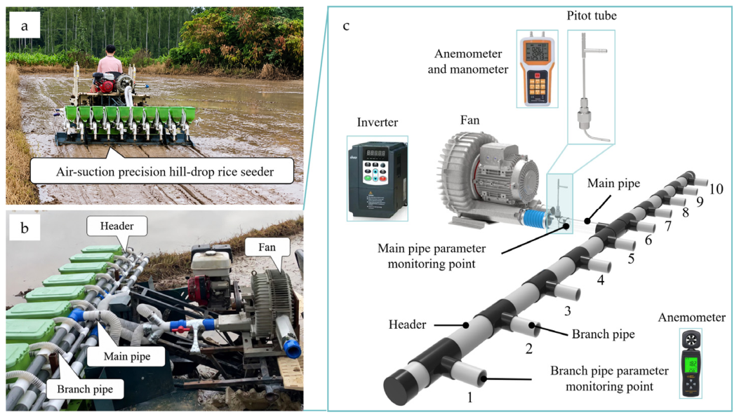
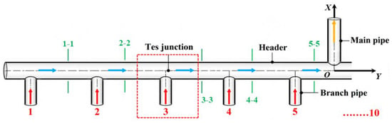
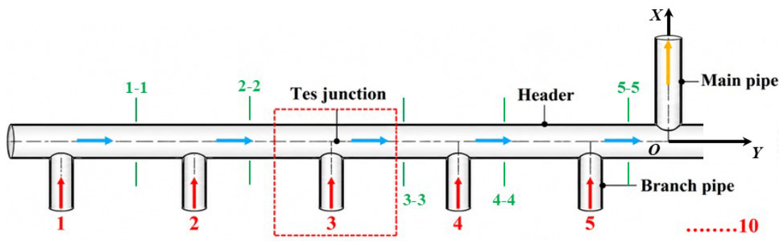
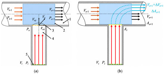
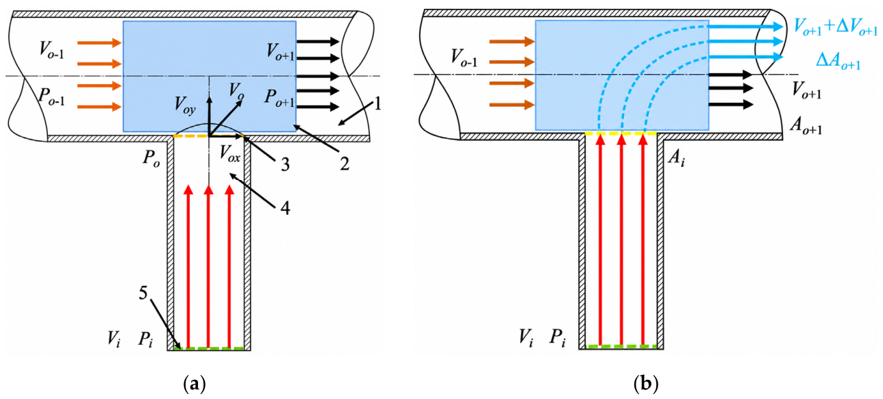
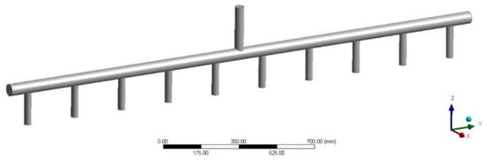
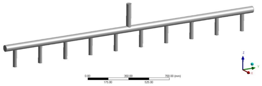
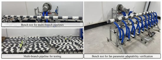
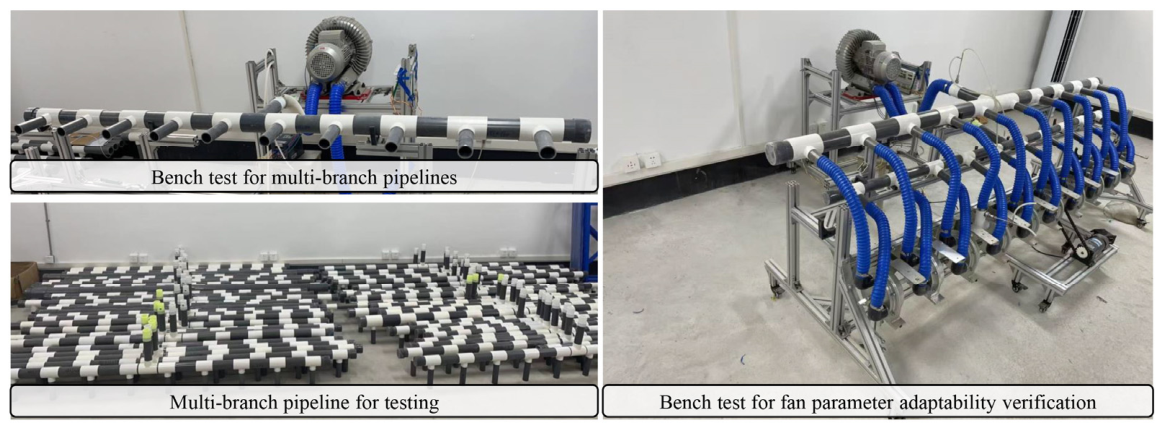

Disclaimer/Publisher’s Note: The statements, opinions and data contained in all publications are solely those of the individual author(s) and contributor(s) and not of MDPI and/or the editor(s). MDPI and/or the editor(s) disclaim responsibility for any injury to people or property resulting from any ideas, methods, instructions or products referred to in the content. |
© 2026 by the authors. Licensee MDPI, Basel, Switzerland. This article is an open access article distributed under the terms and conditions of the Creative Commons Attribution (CC BY) license.