


Abstract
Pineapple is an economically important tropical fruit crop that contributes substantially to agricultural production, international trade, and rural livelihoods in tropical regions. Pineapple can be planted throughout the year under favorable climatic conditions, resulting in strong phenological asynchrony among fields and reducing the effectiveness of conventional fixed-window classification. To address this challenge, this study proposes a phenology-guided dynamic temporal window approach for pineapple mapping using Sentinel-2 time-series observations. A continuous normalized difference vegetation index (NDVI) time series was reconstructed to identify the start of the growing season (SOS) for individual fields, which was then used as a temporal reference to define a key phenological window 12–14 months after the SOS, corresponding to the inflorescence emergence and flowering stages. Nine multispectral bands and seven vegetation indices within this window were summarized and used to train a random forest classifier. Experiments in Xuwen County, China, showed that the proposed method achieved an overall accuracy of 91.67% and a Kappa coefficient of 0.8329, with pineapple producer’s accuracy, user’s accuracy, and F1-score of 90.44%, 92.04%, and 91.23%, respectively. Compared with a conventional fixed-window approach, overall accuracy increased from 85.83% to 91.67%, demonstrating the benefit of phenological alignment. Shortwave-infrared bands and moisture-related indices contributed most strongly to classification. Regional application produced a pineapple distribution map broadly consistent with known planting patterns. These results demonstrate that aligning asynchronously planted fields to comparable phenological stages can improve spectral feature consistency and support accurate regional pineapple mapping.
1. Introduction
Pineapple (Ananas comosus) is one of the most economically important tropical fruit crops worldwide and plays an important role in both domestic food markets and international agricultural trade. According to the Food and Agriculture Organization (FAO), pineapple is the second most exported tropical fruit after banana [1]. It is widely cultivated across tropical and subtropical regions, with major production concentrated in countries such as Costa Rica, the Philippines, Brazil, Thailand and China [2]. The continued expansion of pineapple production and consumption has increased the demand for timely and accurate information on its planting area and spatial distribution, which is essential for agricultural management, production estimation and industry planning. Conventional crop acreage surveys are labor-intensive and inefficient for large-area monitoring [3]. Satellite remote sensing provides a more efficient approach for large-scale crop mapping, making it well-suited for monitoring pineapple planting areas [4,5].
Early studies on pineapple mapping primarily relied on single-date optical imagery, in which pineapple was distinguished from other land-cover or crop types based mainly on spectral and spatial differences at a specific observation time. For example, Tan [6] used Landsat satellite imagery and the Spectral Angle Mapper (SAM) method to identify pineapple plantations in Xuwen County, Zhanjiang, Guangdong Province. Panboonyuen et al. [7] designed a mixed-scale convolutional feedforward network and developed a Vision Transformer-based semantic segmentation model for medium-resolution imagery. Using Landsat satellite imagery, they distinguished rubber trees, pineapples, and maize in Nan Province, Thailand. However, single-date imagery captures crop characteristics only at a specific observation time and may therefore provide limited information on crop development over the growing cycle.
Phenological features provide valuable information for crop identification by capturing differences in crop growth trajectories that may not be evident from single-date imagery. Previous studies have demonstrated that integrating phenological information from multi-temporal observations can substantially improve the classification of crops [8,9,10]. For instance, Chen et al. [11] used Sentinel-2 time-series observations, together with harmonic regression and random forest classification, to map multiple tropical crops, including pineapple, at 10 m resolution in eastern Thailand, demonstrating the potential of temporal growth patterns for tropical crop discrimination. Aduvukha et al. [12] integrated multi-temporal Sentinel-2 spectral bands, vegetation indices, and phenological features with Sentinel-1 backscatter data and used a random forest model to map the cropping patterns of multiple crops, including pineapple. Dense remote-sensing time series can further characterize crop growth trajectories and derive phenological metrics such as the start and end of the growing season (SOS and EOS), making phenology an increasingly important component of crop mapping [13,14,15,16]. Previous studies have demonstrated the clear advantages of phenology-based crop identification in complex agricultural landscapes with high spatial heterogeneity, highlighting its considerable potential for pineapple mapping. However, existing approaches generally rely on fixed observation periods, time-series features, or conventional phenological metrics, without explicitly accounting for the phenological asynchrony caused by differences in pineapple planting dates.
Unlike many annual crops such as rice, maize and soybean, pineapple is cultivated year-round in tropical regions because of favorable climatic conditions. Consequently, pineapple fields within the same region may simultaneously occur at different phenological stages, including establishment, leaf development, flowering and fruit development [17]. These stages are accompanied by pronounced changes in canopy appearance: leaves exhibit mixed pale-purple and light-green tones during early growth, a distinctive magenta-to-green gradient develops during flowering, and leaf yellowing becomes evident at later stages. Such phenological variability results in substantial intra-class spectral differences among pineapple fields observed at the same calendar date. Consequently, conventional approaches based on fixed temporal windows or temporally unaligned observations may fail to capture comparable phenological characteristics across fields [18,19], highlighting the need for a phenology-aligned dynamic temporal window for pineapple identification.
To address these challenges, this study proposes a phenology-guided dynamic temporal window approach for pineapple mapping. The approach focuses on the inflorescence emergence and flowering stages, during which pineapple exhibits distinctive canopy color characteristics, and dynamically aligns fields with different planting dates to comparable phenological stages. Specifically, Sentinel-2 time-series imagery was used to construct NDVI trajectories and identify the start of the growing season (SOS) for individual fields. The key phenological window was then determined relative to SOS based on pineapple growth characteristics, and multispectral features within this window were extracted for random forest classification. Unlike Huang et al. [8], who used RF-DTW to align soybean time series and evaluated their approach across multiple sites and years, this study defines an SOS-referenced window for pineapple and demonstrates the proposed approach to be more effective for mapping in tropical regions, as evaluated in Xuwen County, Guangdong Province, one of China’s major pineapple-producing regions.
2. Materials
2.1. Study Area
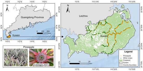
Xuwen County (20°13′ N–20°43′ N, 109°52′ E–110°35′ E), Zhanjiang City, Guangdong Province, China was selected as the study area (Figure 1). Located at the southern tip of mainland China, Xuwen County covers an area of 1987.9 square kilometers. In 2024, the pineapple cultivation area was 21,829.87 ha, with a yield of 792,198 metric tons and a production value of RMB 5.43 billion, making it the largest pineapple-producing region in China [20]. Xuwen County lies in the transition zone between tropical and subtropical climates and is strongly influenced by the monsoon climate. The region has a mean annual temperature of approximately 23.3 °C, an annual accumulated temperature above 10 °C of about 8652.2 °C, and approximately 2000 h of sunshine per year. Mean annual precipitation is approximately 1383 mm, with hot and rainy summers and warm winters. These favorable hydrothermal and radiation conditions provide sufficient energy and moisture for year-round pineapple growth, photosynthesis, and carbohydrate accumulation.
Figure 1.
Geographical location of the study area (the pineapple flowering image was sourced from Catasges [21]).
2.2. Sentinel-2 Time-Series Dataset
This study obtained Sentinel-2 multispectral instrument Level-2A (L2A) spectral reflectance data from the Google Earth Engine (GEE) platform (https://earthengine.google.com/, accessed on 25 June 2026), using the COPERNICUS/S2_SR_HARMONIZED image collection. The Sentinel-2 constellation comprises Sentinel-2A and Sentinel-2B, both operating in sun-synchronous orbits with a revisit interval of 10 days for a single satellite and approximately 5 days when combined. The multispectral instrument provides 13 spectral bands at spatial resolutions of 10 m for the visible and near-infrared bands, 20 m for the red-edge and shortwave-infrared bands, and 60 m for bands primarily used for atmospheric correction. With a swath width of 290 km, Sentinel-2 provides frequent observations over large areas. To ensure full coverage of the pineapple growth cycle, Sentinel-2 imagery acquired from January 2023 to December 2025 was collected, and scenes with cloud cover below 20% were retained, resulting in 42 valid scenes. The 20 m red-edge and SWIR bands were resampled to 10 m using the nearest-neighbor method before vegetation index calculation to ensure a consistent spatial resolution across all spectral features. The spectral characteristics and spatial resolutions of the Sentinel-2 multispectral bands, together with their relevant information for this study, are summarized in Table 1.
Table 1.
Sentinel-2 multispectral instrument spectral bands and their key information.
2.3. Sample Data
The pineapple and non-pineapple samples used in this study were collected through field surveys conducted in Xuwen County in July 2024 and supplemented by visual interpretation of high-resolution Google Earth imagery. A total of 1547 samples were selected, including 650 pineapple samples and 897 non-pineapple samples (Figure 1). Each sample point represented a distinct agricultural field, with only one sample point selected per field. The pineapple samples covered fields at multiple growth stages, thereby capturing the phenological variability associated with different planting times. The non-pineapple class included sugarcane, banana, pitaya, eucalyptus, and other locally common crop types. To minimize mixed-pixel effects, sample locations were placed as close as possible to the centers of individual fields. After quality screening, 400 SOS-valid samples from each class were randomly selected to form a balanced set of 800 samples in each experimental run, which was then divided by stratified random sampling into 560 training samples and 240 held-out test samples (70:30). The same sampling and splitting procedure was used for the dynamic-window and fixed-window experiments.
3. Methods
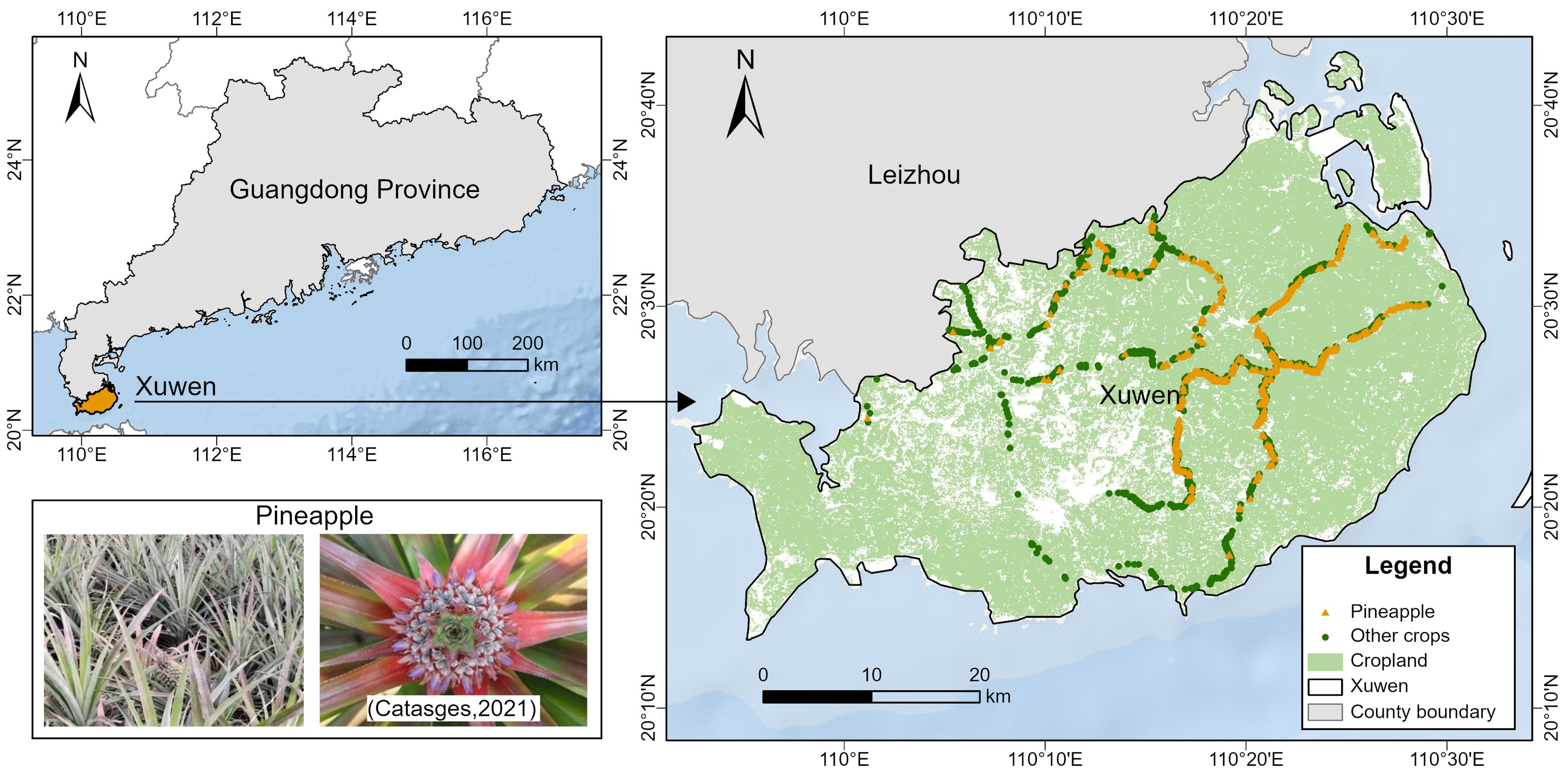
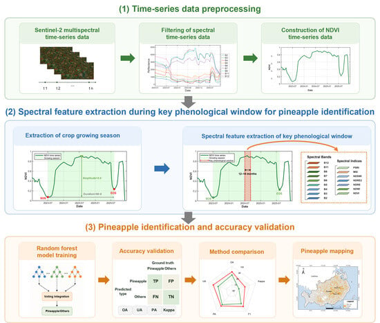
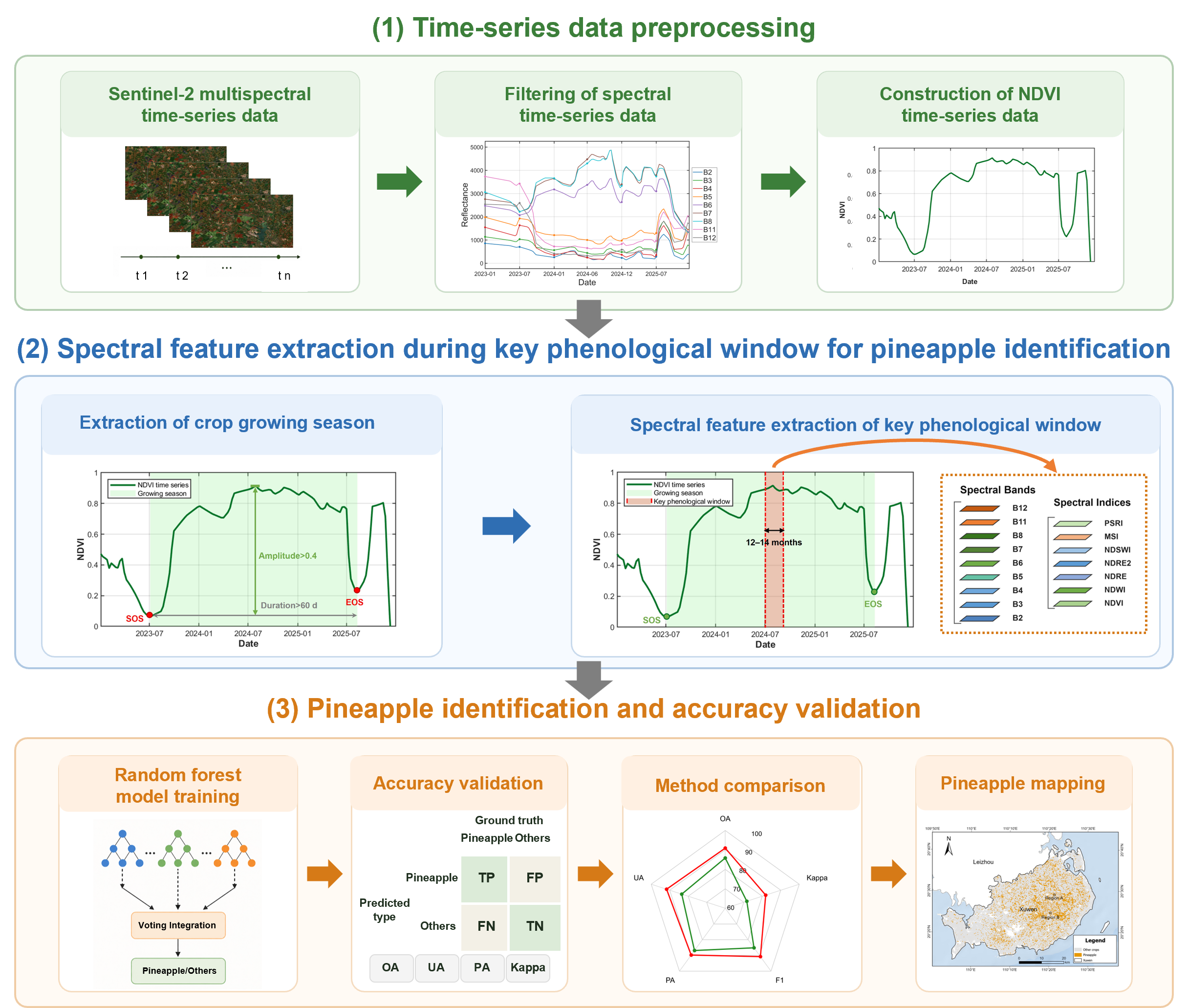
The overall methodological framework consisted of three main steps (Figure 2). First, Sentinel-2 multispectral time-series data were preprocessed to remove unreliable observations and reconstruct continuous spectral trajectories, from which NDVI time series were generated. Second, crop growing seasons were identified from the NDVI trajectories, and a phenology-guided key temporal window was dynamically determined for each sample. Multispectral bands and spectral indices within this window were then extracted to construct the feature set for pineapple identification. Third, a random forest classifier was trained using the extracted features, followed by accuracy assessment and comparison with a conventional fixed-window approach. Finally, the validated model was applied to map the spatial distribution of pineapple plantations across the study area.
Figure 2.
Methodological framework.
3.1. Time-Series Data Preprocessing
First, pixel-level cloud masking was applied to the Sentinel-2 L2A imagery using the cloud probability band and the Scene Classification Layer (SCL). Pixels with cloud probabilities below 5% were retained, while those classified as cloud shadows or cirrus in the SCL were excluded. The resulting cloud-filtered imagery was then used to extract spectral time-series data.
To further reduce anomalous fluctuations in the time series caused by residual clouds and shadows, an outlier detection procedure was applied to improve data quality. For each observation, a three-point local temporal window was constructed, with the mean of the preceding and subsequent observations used as the reference value for the central observation. The deviation between the observed and reference values was then calculated to identify anomalously low observations. Specifically, an observation was considered an outlier when its value decreased by more than 0.20 relative to the reference value and the adjacent observations were acquired within 14 days, or when the decrease exceeded 0.40 within a 21-day interval. Identified outliers were replaced with the corresponding reference values to reduce abrupt fluctuations caused by residual cloud and shadow contamination. Subsequently, missing observations were filled using linear interpolation to ensure the continuity of the time series. The reconstructed time series were then smoothed using the Savitzky–Golay (S-G) filter [22] to reduce residual noise while preserving the temporal variation in spectral signals. A second-order polynomial with a five-observation moving window was used for local fitting. Finally, the smoothed time series were resampled to a regular 8-day interval using linear interpolation, providing temporally consistent observations for subsequent phenological analysis.
3.2. Extraction of Crop Growing Season
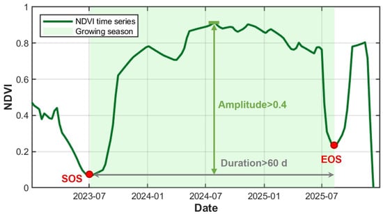
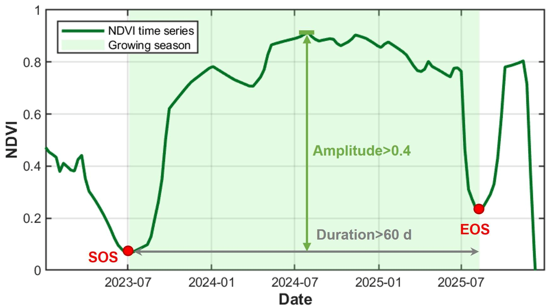
Based on the preprocessed spectral time series, the normalized difference vegetation index (NDVI) was calculated to characterize crop phenological dynamics. During a typical crop growth cycle, NDVI generally increases with canopy development, reaches a maximum, and subsequently declines toward crop maturity or harvest [23]. In this study, a modified threshold-based segmentation method was applied to the NDVI time series to identify individual crop growing seasons (Figure 3). First, all local minima with NDVI values below 0.3 were identified as potential boundaries of the growing season, which represent periods of low vegetation cover or exposed soil. Adjacent local minima were then used to define candidate temporal segments. Each segment was evaluated according to its duration and NDVI amplitude and was considered to represent a complete growing season when the interval between the two local minima exceeded 60 days and the NDVI amplitude was greater than 0.4. The dates corresponding to the two boundaries were subsequently recorded as the start of season (SOS) and end of season (EOS), respectively.
Figure 3.
Extraction of crop growing season based on NDVI time series.
3.3. Spectral Feature Extraction of Key Phenological Window
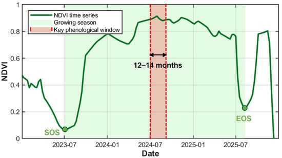
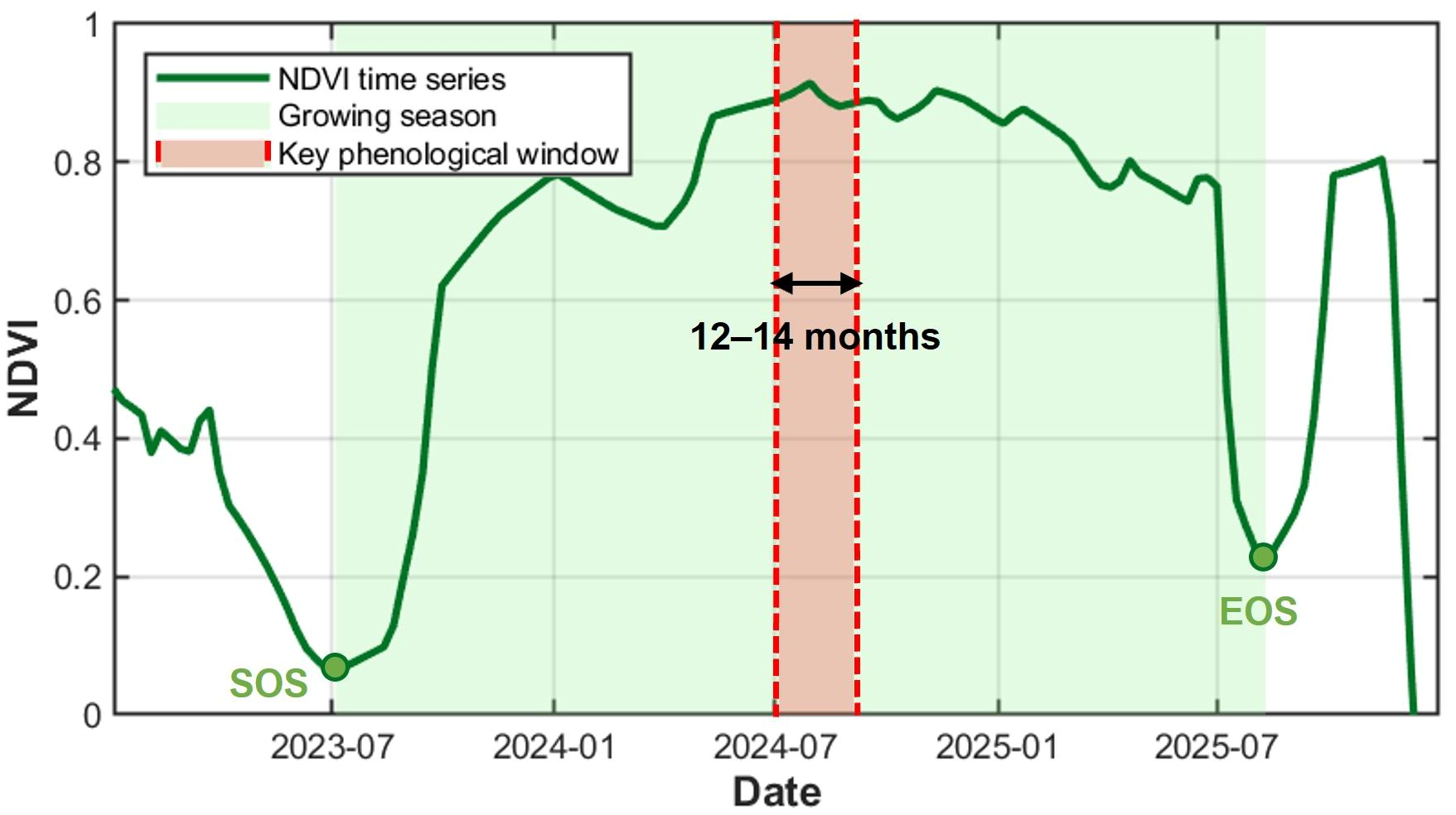
Based on the extracted growing seasons, SOS was used as the temporal reference point, and the period from 12 to 14 months after SOS was defined as the key phenological window for pineapple identification (Figure 4). Spectral reflectance bands and vegetation indices within this window were extracted (Table 2). For each feature, all observations within the window were ranked, and only values between the 25th and 75th percentiles were retained to reduce the influence of extreme observations. The mean of the retained values was then calculated and used as the corresponding input feature for random forest classification.
Figure 4.
Definition of key phenological window for pineapple identification.
Table 2.
Spectral reflectance and vegetation indices.
The spectral information from nine Sentinel-2 bands (B2, B3, B4, B5, B6, B7, B8, B11, and B12) was used for pineapple identification. The visible bands primarily capture variations in vegetation pigments, while the red-edge bands are sensitive to chlorophyll content and vegetation development. The near-infrared band reflects canopy structure and vegetation vigor, whereas the shortwave-infrared bands provide information related to vegetation and soil moisture. Together, these bands provide complementary spectral information that represents the pineapple canopy characteristics more comprehensively for subsequent classification.
Based on the original spectral bands, seven vegetation indices were further derived to characterize crop growth conditions and physiological properties. Among them, the NDVI, one of the most widely used vegetation indices, is effective for characterizing vegetation vigor, fractional cover, and biomass dynamics [24]. The Normalized Difference Red Edge Index (NDRE) exploits the sensitivity of red-edge reflectance to chlorophyll content and is widely used to characterize vegetation chlorophyll status and canopy vigor, particularly under relatively dense vegetation conditions [25]. The Normalized Difference Red Edge Index 2 (NDRE2), which combines near-infrared and red-edge information, provides enhanced sensitivity to high-biomass vegetation and can improve spectral discrimination among crop types [26].
The Normalized Difference Water Index (NDWI) was used to characterize variations in vegetation canopy water content and is sensitive to crop water status [27]. The Normalized Difference Shortwave Infrared Index (NDSWI), which incorporates shortwave-infrared information, reflects differences in vegetation and soil moisture and can help distinguish vegetation under different growth conditions [28]. The Moisture Stress Index (MSI), derived from the ratio of near-infrared to shortwave-infrared reflectance, is sensitive to changes in vegetation water stress and crop moisture status [29]. The Plant Senescence Reflectance Index (PSRI) combines visible and red-edge reflectance to capture changes in leaf pigment composition and is therefore useful for characterizing vegetation senescence and physiological conditions [30].
3.4. Pineapple Identification
This study used a random forest model for pineapple identification. Random forest is a typical ensemble learning method that constructs multiple decision trees by applying Bagging (Bootstrap Aggregating) to the training samples. During model training, TreeBagger uses bootstrap sampling with replacement to construct training samples for each decision tree. At each node split, it randomly selects a subset of features from which the optimal split is determined, thereby enhancing the diversity among decision trees and improving the model’s generalization ability. Finally, the sample class is determined through a majority voting mechanism to make classification decisions [31]. Furthermore, this study employs the Out-of-Bag (OOB) method combined with Permutation Importance to evaluate feature importance. This method measures a feature’s contribution to classification results by randomly permuting the value of a specific feature in the out-of-bag sample and comparing the change in the model’s prediction error before and after the permutation; the greater the increase in error, the higher the importance of that feature [32].
The random forest classifier was implemented in MATLAB R2024a using the TreeBagger function. The number of trees was set to 300, and the minimum leaf size was set to 5; other TreeBagger parameters retained their default values. A fixed random seed (rng(20260828)) was used. To assess model stability and reduce the influence of random data partitioning, the classification procedure was repeated 100 times. Classification performance and feature importance scores were recorded for each run and subsequently summarized across all repetitions.
3.5. Accuracy Validation
To evaluate the classification performance of the model, a confusion matrix and its derived metrics were used for accuracy assessment, including overall accuracy (OA), user’s accuracy (UA), producer’s accuracy (PA), F1-score, and the Kappa coefficient. UA measures the reliability of the predicted class, whereas PA reflects the ability of the model to correctly identify samples belonging to a given class. OA represents the proportion of correctly classified samples among all validation samples. The F1-score, calculated as the harmonic mean of precision and recall, provides a balanced measure of classification performance, particularly when class distributions are uneven. The Kappa coefficient was further used to quantify the agreement between predicted and reference labels while accounting for agreement expected by chance.
3.6. Comparative Experiment
To evaluate the effectiveness of the proposed dynamic temporal window approach, a conventional pineapple classification method based on a fixed temporal window was designed as a comparative experiment. Under the same random forest configuration, pineapple and non-pineapple samples were classified using Sentinel-2 multispectral features extracted from a fixed observation period. Specifically, Sentinel-2 images acquired between January 2024 and December 2025 were selected and processed using cloud masking, after which a median composite was generated for the study area. The same nine spectral bands (B2, B3, B4, B5, B6, B7, B8, B11, and B12) and seven spectral indices (NDVI, NDWI, NDRE, NDRE2, NDSWI, MSI, and PSRI) were extracted, resulting in a 16-dimensional feature set. Classification performance was evaluated using OA, UA, PA, F1-score, and the Kappa coefficient.
4. Results
4.1. NDVI Temporal Patterns of Typical Crops
Figure 5 and Figure 6 present the NDVI time series of pineapple and other typical crops in the study area.
Figure 5.
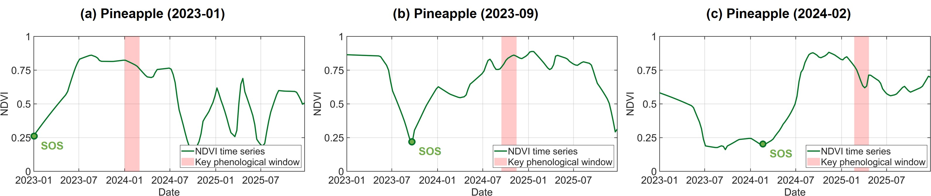
NDVI time series of pineapple fields with different planting dates. The extracted phenological windows are shown in the figures: (a) Pineapple (SOS: 2023-01), (b) Pineapple (SOS: 2023-09), (c) Pineapple (SOS: 2024-02).
Figure 6.
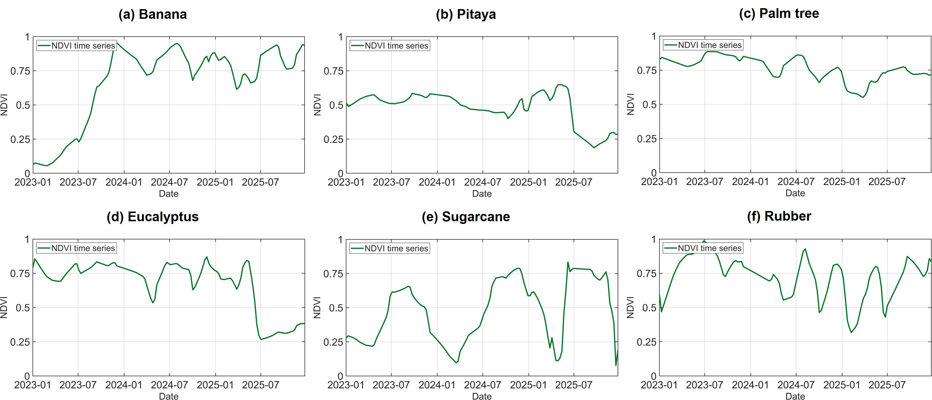
NDVI time series of other typical crops in the study area. (a) Banana, (b) Pitaya, (c) Palm tree, (d) Eucalyptus, (e) Sugarcane, (f) Rubber.
Figure 5 shows the NDVI time series of pineapple fields with different planting dates. The three pineapple samples exhibited pronounced differences in the timing of NDVI increase, peak greenness, and subsequent decline, indicating substantial temporal variability among fields. Pineapple generally has a growth cycle longer than 18 months, spanning vegetative growth, floral differentiation, flowering, fruit development, and maturation. Consequently, its growing season often extends across calendar years and is considerably longer than that of typical annual crops. In Figure 5, the green circles indicate the low-NDVI points identified as the approximate planting or establishment dates of individual pineapple fields. Although these dates differed markedly among the three samples, each field subsequently exhibited a sustained increase in NDVI followed by a relatively long period of high vegetation cover. The red bars represent the dynamic phenological windows defined at 12–14 months after planting. Because these windows shift according to the planting date of each field, they occur at different calendar dates but correspond to comparable stages of pineapple development. This phenological alignment reduces the temporal mismatch caused by asynchronous planting and enables spectral features to be extracted from a more consistent growth stage across pineapple fields.
Figure 6 presents the NDVI time series of representative non-pineapple crops in the study area, including banana, pitaya, palm tree, eucalyptus, sugarcane, and rubber. Distinct temporal patterns were observed among crop types. Sugarcane showed pronounced cyclical dynamics, with NDVI increasing rapidly during vegetative growth and declining sharply after maturity or harvest. Banana generally maintained relatively high NDVI values after canopy establishment, but exhibited repeated short-term fluctuations, reflecting its prolonged and less clearly defined growth cycle. Pitaya showed comparatively small seasonal variations and remained at a moderate NDVI level for most of the observation period. In contrast, palm tree and eucalyptus maintained relatively high NDVI values during some periods but also exhibited marked declines associated with changes in canopy condition. Rubber displayed strong seasonal fluctuations, characterized by alternating periods of high and low NDVI, consistent with recurrent leaf shedding and canopy recovery.
Despite these contrasting temporal patterns, partial similarities were observed between pineapple and several other crop types during specific growth stages. In particular, banana and pineapple both maintained relatively high vegetation cover over extended periods, resulting in overlapping NDVI ranges during much of their growth cycles. These temporal overlaps indicate that NDVI trajectories alone may not always provide sufficient separability between pineapple and other crops, further supporting the use of phenologically aligned multispectral features for pineapple identification.
4.2. Spectral Separability Within the Dynamic Phenological Window
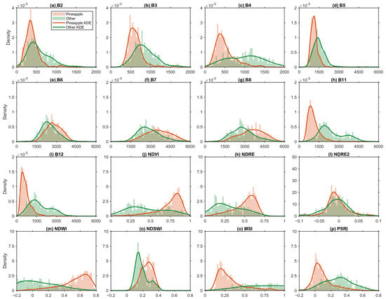
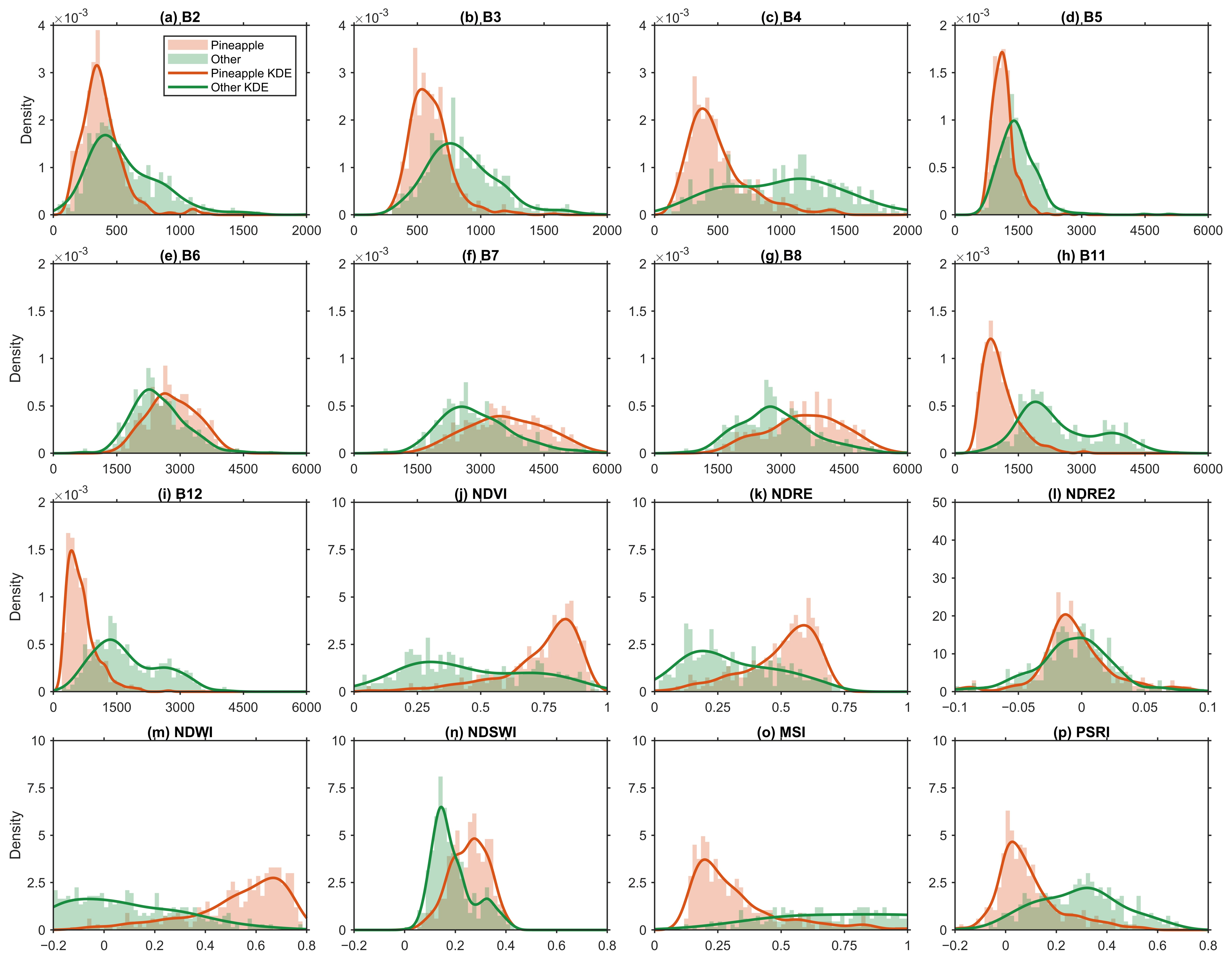
Figure 7 shows the distributions of the spectral features extracted within the dynamic phenological window for pineapple and non-pineapple samples. The histograms represent the frequency distributions of individual features, while the kernel density estimation (KDE) curves illustrate their overall distribution patterns. Clear differences between pineapple and non-pineapple samples were observed for several spectral bands and vegetation indices, indicating that the phenologically aligned window effectively captured discriminative spectral characteristics of pineapple.
Figure 7.
Distributions of spectral features extracted within the dynamic phenological window for pineapple and non-pineapple samples: (a) B2, (b) B3, (c) B4, (d) B5, (e) B6, (f) B7, (g) B8, (h) B11, (i) B12, (j) NDVI, (k) NDRE, (l) NDRE2, (m) NDWI, (n) NDSWI, (o) MSI, (p) PSRI.
Among the original spectral bands, B11 and B12 exhibited the most pronounced separation between the two classes, with pineapple samples generally showing substantially lower reflectance than non-pineapple samples. B4 and B5 also showed noticeable differences, whereas greater distributional overlap was observed for B2, B3, B6, B7, and B8, indicating relatively weaker individual separability. Among the vegetation indices, NDVI, NDRE, NDWI, MSI, and PSRI showed clear differences between pineapple and non-pineapple samples. In particular, pineapple samples were generally characterized by higher NDVI, NDRE, and NDWI values and lower MSI and PSRI values. By contrast, NDRE2 exhibited substantial overlap between the two classes, suggesting limited discriminatory ability when used independently. NDSWI showed intermediate separability.
Overall, the results demonstrate that the dynamic phenological window enhances the spectral contrast between pineapple and other crops, particularly in the shortwave-infrared bands and vegetation indices related to canopy greenness, moisture status, and senescence. The complementary information provided by these features forms a strong basis for subsequent random forest classification.
4.3. Classification Accuracy Assessment
Table 3 presents the mean confusion matrix and associated accuracy metrics for the proposed method.
Table 3.
Confusion matrix and classification accuracy of the proposed method.
The model achieved an OA of 91.67% and a Kappa coefficient of 0.8329, indicating strong agreement between the predicted and reference classes. For pineapple, the PA, UA, and F1-score were 90.44%, 92.04%, and 91.23%, respectively. For other crops, the corresponding values were 92.80%, 91.34%, and 92.07%. These results demonstrate that the proposed model effectively distinguished pineapple from other crops with high and balanced classification accuracy. The high performance further suggests that the multispectral features extracted within the key phenological window captured discriminative characteristics of pineapple, providing a reliable basis for subsequent regional-scale pineapple mapping.
4.4. Feature Importance Analysis
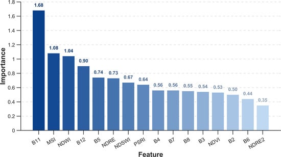
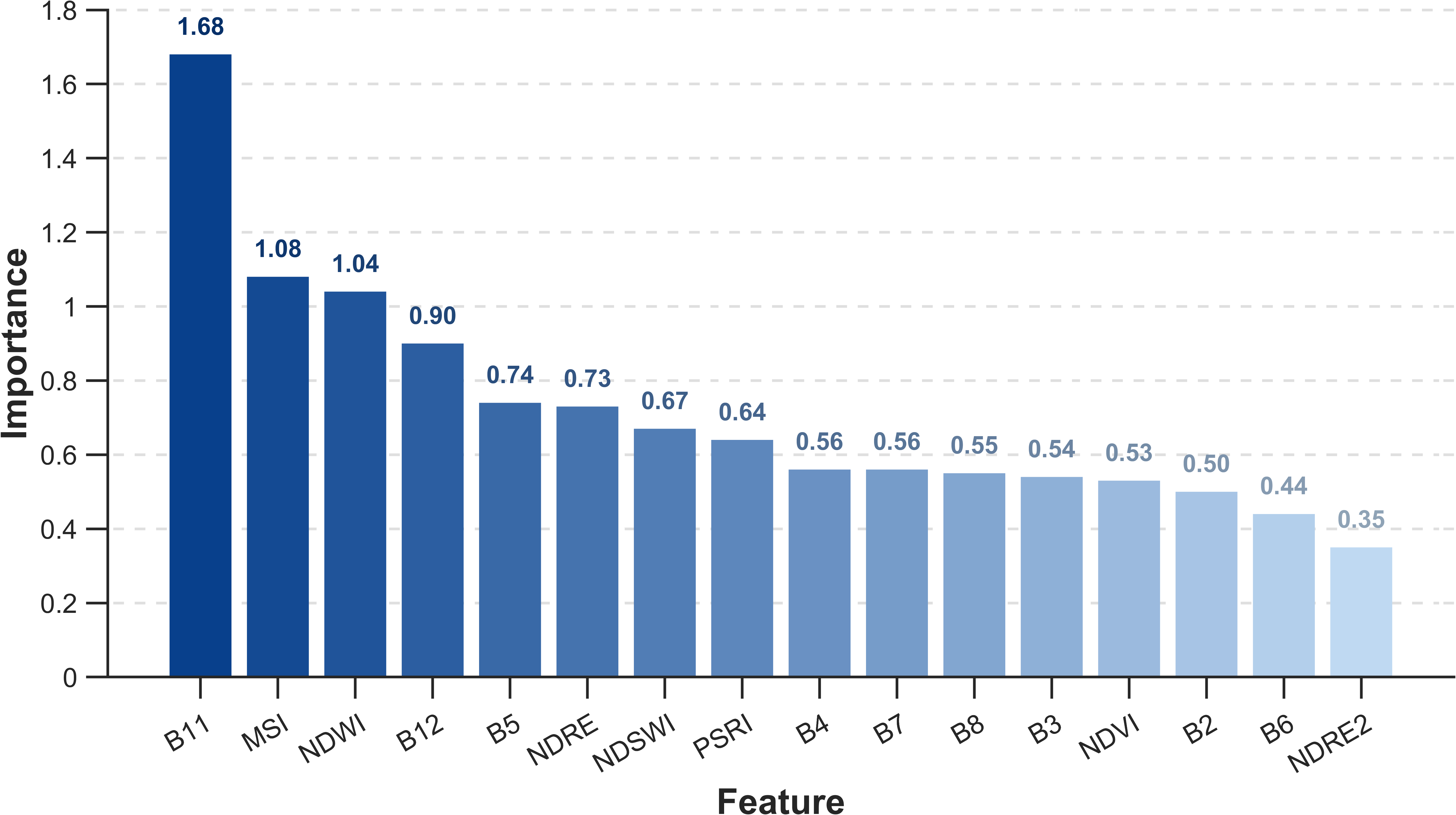
The importance of the 16 input features in pineapple classification is shown in Figure 8. Overall, feature importance exhibited a clear ranking, indicating substantial differences in the contributions of individual spectral features to classification. Among all features, the shortwave-infrared band B11 showed the highest mean importance score (1.68), markedly exceeding the other variables. MSI and NDWI ranked second and third, with importance scores of 1.08 and 1.04, respectively, followed by B12 (0.90), B5 (0.74), NDRE (0.73), and NDSWI (0.67).
Figure 8.
Ranking of feature importance.
Notably, B11 (1539–1682 nm) and B12 (2078–2320 nm) are both located in the SWIR region and are sensitive to variations in vegetation water content. Their relatively high importance, together with the high rankings of the water-related indices MSI and NDWI, indicates that moisture-related spectral information played a major role in distinguishing pineapple from other crops. The red-edge band B5 (698–713 nm) and NDRE also showed relatively high importance, suggesting that spectral responses associated with chlorophyll status and canopy development provided complementary information for pineapple discrimination. In contrast, B6 and NDRE2 showed the lowest importance scores, indicating comparatively limited contributions to the classification model. During pineapple flowering, changes in leaf color may cause pronounced variations in red band B4 reflectance, thereby enhancing spectral separability from other green vegetation.
Overall, during floral bud development, pineapple leaves gradually develop reddish coloration from the basal region, accompanied by changes in leaf water status. These physiological changes may enhance the sensitivity of SWIR bands and moisture-related indices, making them particularly informative for pineapple discrimination. Accordingly, SWIR bands and their derived moisture indices constituted the core feature set for pineapple classification, while red-edge features provided complementary information related to chlorophyll status and canopy development. Together, these spectral characteristics enhanced the separability between pineapple and other crops.
4.5. Pineapple Mapping
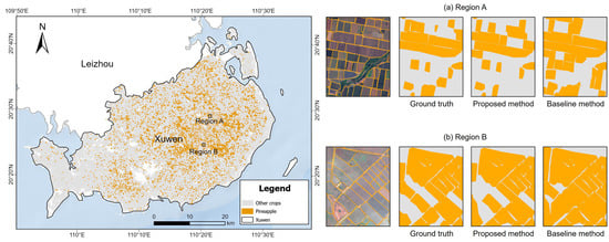
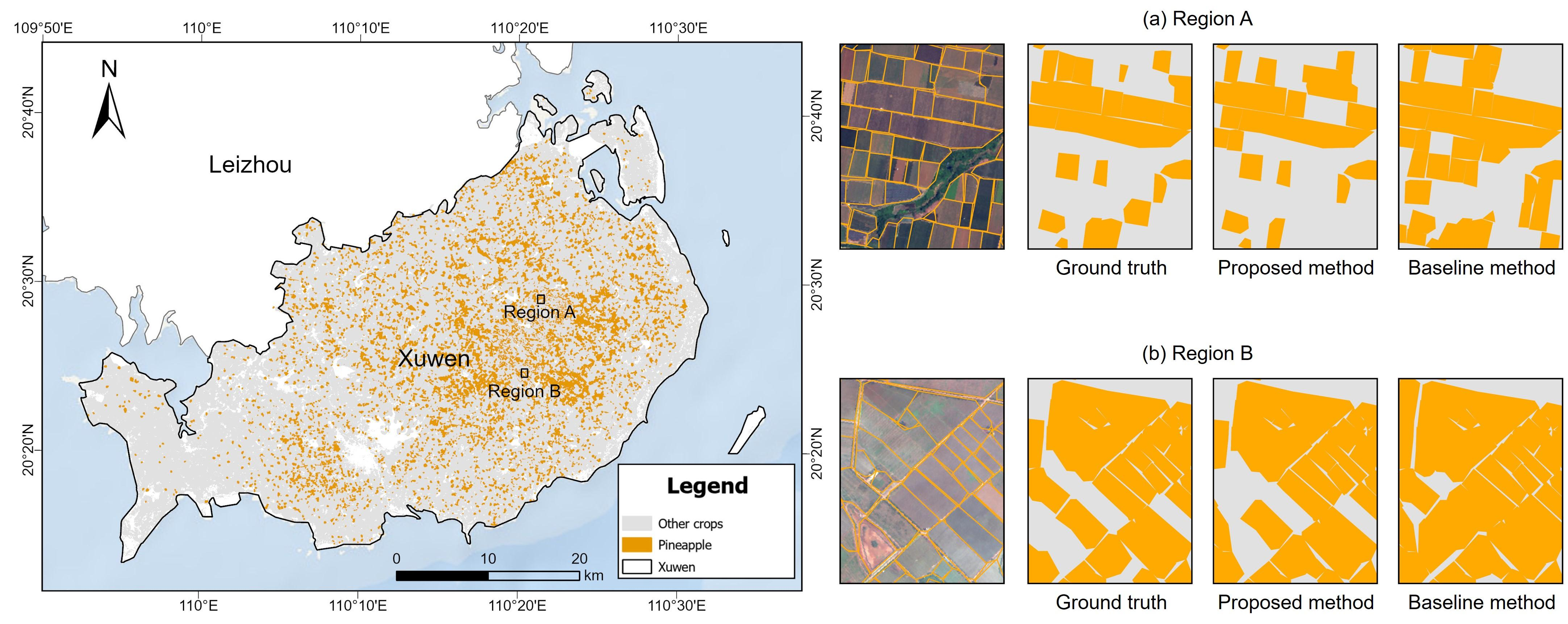
The trained random forest model was applied to Sentinel-2 imagery across Xuwen County to generate the pineapple plantations. Pre-existing agricultural parcel boundaries were used as the basic spatial units for pineapple classification and mapping. The mapping results (Figure 9) showed that pineapple plantations were mainly concentrated in Qujie Town in central Xuwen, Longtang Town in the southeast, and Nanshan Town and surrounding agricultural farm areas in the central-western part of the county. These plantations generally exhibited spatially clustered distributions, whereas relatively fewer pineapple fields were identified in the southwestern part of the study area. Overall, the mapped distribution was broadly consistent with the known agricultural planting pattern of Xuwen County.
Figure 9.
Pineapple mapping in Xuwen County (from left to right: ground truth, proposed method, baseline method).
Based on the classification results, the total pineapple planting area was estimated to be approximately 17,693.614 ha. According to the 2024 Statistical Communiqué on the National Economic and Social Development of Xuwen County, the officially reported pineapple planting area was 21,829.8667 ha. The remote-sensing estimate accounted for 81.05% of the reported area, corresponding to a relative error of 18.95% and indicating an overall underestimation of pineapple planting area [20]. The discrepancy between the two estimates may arise from several sources. First, agricultural statistics and remote-sensing-based estimates differ in their data sources and statistical definitions. Second, the spatial resolution of Sentinel-2 and mixed-pixel effects may result in the omission of small, fragmented, or mixed-cropping pineapple fields. Third, residual cloud contamination, time-series reconstruction, and classification errors may also contribute to underestimation. Despite these differences, the mapped spatial pattern was broadly consistent with the regional distribution of pineapple cultivation, indicating the potential of the proposed method for regional-scale pineapple mapping.
4.6. Performance of Comparative Experiment
The classification performance of the conventional approach based on a fixed temporal window is presented in Table 4.
Table 4.
Confusion matrix and classification accuracy of the comparative method.
The model achieved an overall accuracy of 85.83% and a Kappa coefficient of 0.7167, indicating that multispectral information from a fixed temporal window can provide reasonably good performance for pineapple identification. For the pineapple class, the PA, UA, and F1-score were 84.68%, 87.50%, and 86.07%, respectively. Compared with these results, the proposed dynamic phenological window approach achieved consistently higher accuracy across all evaluation metrics, demonstrating its advantage over the conventional fixed-window method for pineapple classification.
5. Discussion
5.1. Phenological Alignment Improves Pineapple Identification
Pineapple can be planted throughout the year, causing substantial phenological differences among fields observed on the same calendar date. This asynchrony leads to temporal and spectral variability within the pineapple class, thereby reducing the effectiveness of fixed-window observations for classification. The proposed approach addresses this problem by using the start of season as a temporal reference and dynamically locating the key phenological window at 12–14 months after crop establishment. In this way, pineapple fields planted at different dates can be aligned to comparable developmental stages before spectral features are extracted. The effectiveness of this strategy was supported by the comparative experiment. The proposed method achieved an overall accuracy of 91.67% and a Kappa coefficient of 0.8329, compared with 85.83% and 0.7167, respectively, for the conventional fixed-window method. For pineapple specifically, PA increased from 86.87% to 90.44%, UA from 83.50% to 92.04%, and F1-score from 85.15% to 91.23%. These improvements indicate that phenological alignment reduces the temporal mismatch among fields and enables more representative spectral characteristics to be extracted for pineapple identification in tropical agricultural regions.
5.2. Spectral Characteristics Within the Key Phenological Window
The spectral distribution and feature-importance analyses further revealed that the discriminatory information within the dynamic phenological window was not evenly distributed among spectral variables. The SWIR band B11 showed the highest feature importance, followed by MSI and NDWI. These results indicate that spectral information related to vegetation water status played a particularly important role in separating pineapple from other crops. Red-edge information provided additional discriminatory information. B5 and NDRE ranked relatively high in feature importance, suggesting that spectral responses associated with chlorophyll status and canopy development complemented the moisture-sensitive SWIR features. During the floral bud development and flowering stages, pineapple undergoes pronounced changes in leaf color and physiological condition. Such changes can alter both pigment-related and moisture-related spectral responses. More broadly, recent research on large-scale spatiotemporal forecasting has reported that a mismatch between spatial complexity and temporal context can be associated with greater prediction uncertainty, while accounting for temporal heterogeneity may help mitigate cumulative errors [33]. Therefore, concentrating feature extraction within this phenologically comparable stage increases the likelihood of capturing pineapple-specific spectral characteristics, whereas observations acquired outside this period may contain less distinctive or more variable signals.
5.3. Regional Applicability of the Proposed Method
The proposed approach was further applied at the field level across Xuwen County to generate a regional pineapple distribution map. The mapped pineapple plantations were mainly concentrated in the central, southeastern, and central-western parts of the county, broadly corresponding to the major pineapple-producing areas. The spatially clustered distribution detected by the model was consistent with the known agricultural planting pattern of the study area, demonstrating the potential of the approach for operational pineapple mapping.
The total mapped pineapple area was approximately 17,693.614 ha, compared with the officially reported area of 21,829.8667 ha in 2024. This corresponds to a relative error of 18.95%, with the remote-sensing estimate showing an overall underestimation. Several factors may contribute to this discrepancy. Agricultural statistics and remote-sensing estimates are based on different data sources and statistical definitions, while the spatial resolution of Sentinel-2 may limit the detection of small, fragmented, or mixed-cropping fields. Residual cloud contamination, time-series reconstruction, and classification errors may further contribute to omissions. Nevertheless, the overall spatial agreement and relatively high sample-based classification accuracy indicate that the proposed approach has potential for regional-scale pineapple inventory and monitoring.
5.4. Limitations and Future Work
Several limitations should be considered. First, this study relied primarily on optical Sentinel-2 observations. Frequent cloud cover in tropical regions can reduce the temporal continuity of optical observations, and although outlier removal, interpolation, and S-G filtering were used to reconstruct the time series, these procedures may introduce uncertainty or smooth some original spectral information [34]. Future studies could integrate Sentinel-1 SAR observations with Sentinel-2 data to improve temporal completeness and provide complementary structural information under cloudy conditions [35]. Disease or other environmental stresses may cause abnormal NDVI declines, potentially leading to misidentification of phenological transitions and errors in SOS detection.
Second, the present approach focused on a single key phenological window. Although this window effectively captured distinctive pineapple characteristics, the complete pineapple growth cycle contains multiple developmental stages with different physiological and spectral properties. Future studies could extend the current framework to multiple phenological windows, thereby integrating complementary information from vegetative development, floral differentiation, flowering, fruit development, and maturation. Meteorological variables and accumulated temperature could also be incorporated to improve the physiological basis and transferability of phenological alignment [36]. Although the phenological alignment framework may be adapted to other crops by using crop-specific SOS as a temporal anchor, the 12–14-month window defined in this study is specific to pineapple and should not be directly applied to other crops without recalibrating the temporal relationship between SOS and the target developmental stage.
Third, the samples used in this study were primarily collected from one major pineapple-producing region and within a limited temporal period. Differences in cultivar, planting practices, climate, and management may alter pineapple phenology and spectral responses in other regions. Consequently, the robustness of the 12–14-month window requires further evaluation across multiple years and geographic regions. Expanding field samples and incorporating multi-year observations will therefore be important for assessing model transferability. More advanced time-series models, including deep-learning approaches, could also be explored to capture more complex temporal patterns and further improve regional generalization [18].
6. Conclusions
This study developed a phenology-guided dynamic temporal window approach for pineapple mapping using Sentinel-2 time-series observations. By identifying crop establishment from NDVI trajectories and extracting multispectral features within a key window 12–14 months after the start of the growing season, the method aligned pineapple fields with different planting dates to comparable phenological stages. The resulting random forest model achieved an overall accuracy of 91.67%, a Kappa coefficient of 0.8329, and pineapple PA, UA, and F1-score values of 90.44%, 92.04%, and 91.23%, respectively, outperforming the conventional fixed-window approach.
SWIR bands and moisture-related indices, particularly B11, MSI, NDWI, and B12, provided the strongest discriminatory information, while red-edge features supplied complementary information related to vegetation physiological status. Regional application in Xuwen County further demonstrated the feasibility of the approach for pineapple mapping. Overall, phenological alignment provides an effective means of reducing temporal variability caused by year-round pineapple planting and improving the consistency of spectral feature extraction. The framework provides a useful basis for large-area pineapple monitoring and could be further strengthened through multi-source remote sensing, multi-stage phenological characterization, and cross-regional validation.
Author Contributions
Conceptualization, J.L., H.L. and Y.Y.; methodology, J.L., H.L. and Y.Y.; validation, J.L., H.L. and Y.Y.; formal analysis, J.L. and H.L.; investigation, J.L., H.L., Y.D. and Q.H.; data curation, Q.H. and B.Q.; writing—original draft preparation, J.L., H.L. and Y.Y.; writing—review and editing, Y.Y., Z.W., Y.D. and J.W.; visualization, J.L., H.L. and X.Y.; supervision, Y.Y.; project administration, Y.Y.; funding acquisition, Y.Y. and B.Q. All authors have read and agreed to the published version of the manuscript.
Funding
This research was funded by Guangdong Basic and Applied Basic Research Foundation (Grant Nos. 2026A1515010868, 2024A1515011854, and 2024B1212080004), the Science and Technology Projects in Guangzhou (Grant 2025A04J4061 and Grant 2025A04J4227), the National Natural Science Foundation of China (Grant 42501491), the National Natural Science Foundation of China (L2424330) and the Science and Technology Program of Guangzhou (2025A03J3171).
Data Availability Statement
The data presented in this study are available from the corresponding author upon reasonable request.
Conflicts of Interest
The authors declare no conflicts of interest.
Abbreviations
The following abbreviations are used in this manuscript:
| GEE | Google Earth Engine |
| MSI | Moisture Stress Index |
| NDRE | Normalized Difference Red Edge Index |
| NDRE2 | Normalized Difference Red Edge Index 2 |
| NDVI | Normalized Difference Vegetation Index |
| NDWI | Normalized Difference Water Index |
| NDSWI | Normalized Difference Shortwave Infrared Index |
| OOB | Out-of-Bag |
| OA | Overall Accuracy |
| PA | Producer’s Accuracy |
| PSRI | Plant Senescence Reflectance Index |
| RF | Random Forest |
| SAR | Synthetic Aperture Radar |
| SCL | Scene Classification Layer |
| S-G | Savitzky–Golay |
| SOS | Start of Season |
| EOS | End of Season |
| UA | User’s Accuracy |
| KDE | Kernel Density Estimation |
References
- Food and Agriculture Organization of the United Nations. Major Tropical Fruits Market Review 2022; FAO: Rome, Italy, 2023. [Google Scholar]
- Sanewski, G.M.; Bartholomew, D.P.; Paull, R.E. The Pineapple: Botany, Production and Uses, 2nd ed.; CABI: Wallingford, UK, 2018. [Google Scholar]
- Atzberger, C. Advances in remote sensing of agriculture: Context description, existing operational monitoring systems and major information needs. Remote Sens. 2013, 5, 949–981. [Google Scholar] [CrossRef] [Scilit]
- Weiss, M.; Jacob, F.; Duveiller, G. Remote sensing for agricultural applications: A meta-review. Remote Sens. Environ. 2020, 236, 111402. [Google Scholar] [CrossRef] [Scilit]
- Abubakar, G.A.; Wang, K.; Koko, A.F.; Husseini, M.I.; Shuka, K.A.M.; Deng, J.S.; Gan, M.Y. Mapping maize cropland and land cover in semi-arid region in Northern Nigeria using machine learning and Google Earth Engine. Remote Sens. 2023, 15, 2835. [Google Scholar] [CrossRef] [Scilit]
- Tan, S.S. Study on Key Techniques of Remote Sensing Estimation of Pineapple Area and Yield in Xuwen County. Master’s Thesis, Guangdong Ocean University, Zhanjiang, China, 2022. [Google Scholar]
- Panboonyuen, T.; Charoenphon, C.; Satirapod, C. MeViT: A medium-resolution vision transformer for semantic segmentation on Landsat satellite imagery for agriculture in Thailand. Remote Sens. 2023, 15, 5124. [Google Scholar] [CrossRef] [Scilit]
- Huang, X.; Vrieling, A.; Dou, Y.; Belgiu, M.; Nelson, A. A robust method for mapping soybean by phenological aligning of Sentinel-2 time series. ISPRS J. Photogramm. Remote Sens. 2024, 218, 1–18. [Google Scholar] [CrossRef] [Scilit]
- Maleki, S.; Baghdadi, N.; Bazzi, H.; Dantas, C.F.; Ienco, D.; Nasrallah, Y.; Najem, S. Machine learning-based summer crops mapping using Sentinel-1 and Sentinel-2 images. Remote Sens. 2024, 16, 4548. [Google Scholar] [CrossRef] [Scilit]
- Htitiou, A.; Boudhar, A.; Lebrini, Y.; Hadria, R.; Lionboui, H.; Benabdelouahab, T. A comparative analysis of different phenological information retrieved from Sentinel-2 time series images to improve crop classification: A machine learning approach. Geocarto Int. 2022, 37, 1426–1449. [Google Scholar] [CrossRef] [Scilit]
- Chen, G.; Hammelman, C.; Anantsuksomsri, S.; Tontisirin, N.; Todd, A.R.; Hicks, W.W.; Robinson, H.M.; Calloway, M.G.; Bell, G.M.; Kinsey, J.E. Fine-scale (10 m) dynamics of smallholder farming through COVID-19 in Eastern Thailand. Remote Sens. 2024, 16, 1035. [Google Scholar] [CrossRef] [Scilit]
- Aduvukha, G.R.; Abdel-Rahman, E.M.; Sichangi, A.W.; Makokha, G.O.; Landmann, T.; Mudereri, B.T.; Tonnang, H.E.Z.; Dubois, T. Cropping pattern mapping in an agro-natural heterogeneous landscape using Sentinel-2 and Sentinel-1 satellite datasets. Agriculture 2021, 11, 530. [Google Scholar] [CrossRef] [Scilit]
- Yang, Y.P.; Zou, J.J.; Huang, Y.; Wu, Z.F.; Fang, T.; Xue, J.; Wang, D.K.; Wang, Y.B.; Wang, J.N.; Yang, X.K.; et al. Investigating the earliest identifiable timing of sugarcane at early season based on optical and SAR time-series data. Remote Sens. 2025, 17, 2773. [Google Scholar] [CrossRef] [Scilit]
- Wang, J.; Xiao, X.; Liu, L.; Wu, X.; Qin, Y.; Steiner, J.L.; Dong, J. Mapping sugarcane plantation dynamics in Guangxi, China, by time series Sentinel-1, Sentinel-2 and Landsat images. Remote Sens. Environ. 2020, 247, 111951. [Google Scholar] [CrossRef] [Scilit]
- Zhang, H.Y.; Zhang, Y.; Tong, F.H.; Li, M.Z. A novel winter wheat yield prediction framework using fused spatial-temporal-spectral (STS) information from Sentinel-2 and Landsat 8 via improved Pix2Pix network. Comput. Electron. Agric. 2025, 231, 109982. [Google Scholar] [CrossRef] [Scilit]
- Li, Y.M.; Liu, X.N.; Liu, M.L.; Wu, L.; Zhu, L.H.; Huang, Z.; Xue, X.J.; Tian, L.W. Historical dynamic mapping of eucalyptus plantations in Guangxi during 1990–2019 based on sliding-time-window change detection using dense Landsat time-series data. Remote Sens. 2024, 16, 744. [Google Scholar] [CrossRef] [Scilit]
- Zhang, H.N.; Sun, W.S.; Sun, G.M.; Liu, S.H.; Li, Y.H.; Wu, Q.S.; Wei, Y.Z. Phenological growth stages of pineapple (Ananas comosus) according to the extended Biologische Bundesantalt, Bundessortenamt and Chemische Industrie scale. Ann. Appl. Biol. 2016, 169, 311–318. [Google Scholar] [CrossRef] [Scilit]
- Zhong, L.H.; Hu, L.N.; Zhou, H. Deep learning based multi-temporal crop classification. Remote Sens. Environ. 2019, 221, 430–443. [Google Scholar] [CrossRef] [Scilit]
- Pelletier, C.; Webb, G.I.; Petitjean, F. Temporal convolutional neural network for the classification of satellite image time series. Remote Sens. 2019, 11, 523. [Google Scholar] [CrossRef] [Scilit]
- Xuwen County Bureau of Statistics. 2024 Statistical Bulletin on National Economic and Social Development of Xuwen County; Xuwen County Bureau of Statistics: Zhanjiang, China, 2025.
- Chinese Academy of Tropical Agricultural Sciences Guangzhou Experimental Station. Pineapple Varieties. Available online: https://www.catasges.cn/contents/2872/215466.html (accessed on 5 July 2026).
- Savitzky, A.; Golay, M. Smoothing and differentiation of data by simplified least squares procedures. Anal. Chem. 1964, 36, 1627–1639. [Google Scholar] [CrossRef] [Scilit]
- Zhang, X.Y.; Friedl, M.A.; Schaaf, C.B.; Strahler, A.H.; Hodges, J.C.F.; Gao, F.; Reed, B.C.; Huete, A. Monitoring vegetation phenology using MODIS. Remote Sens. Environ. 2003, 84, 471–475. [Google Scholar] [CrossRef] [Scilit]
- Rouse, J.W., Jr.; Haas, R.H.; Schell, J.A.; Deering, D.W. Monitoring vegetation systems in the Great Plains with ERTS. In Proceedings of the 3rd ERTS-1 Symposium; NASA Goddard Space Flight Center: Washington, DC, USA, 1973; Volume 1, pp. 309–317. [Google Scholar]
- Gitelson, A.A.; Merzlyak, M.N. Remote sensing of chlorophyll concentration in higher plant leaves. Adv. Space Res. 1998, 22, 689–692. [Google Scholar] [CrossRef] [Scilit]
- Barnes, E.; Clarke, T.; Richards, S.; Colaizzi, P.; Haberland, J.; Kostrzewski, M.; Waller, P.; Choi, C.; Riley, E.; Thompson, T. Coincident detection of crop water stress, nitrogen status and canopy density using ground based multispectral data. In Proceedings of the 5th International Conference on Precision Agriculture, Bloomington, MN, USA, 16–19 July 2000. [Google Scholar]
- Gao, B.-C. NDWI—A normalized difference water index for remote sensing of vegetation liquid water from space. Remote Sens. Environ. 1996, 58, 257–266. [Google Scholar] [CrossRef] [Scilit]
- Hardisky, M.A.; Klemas, V.; Smart, R.M. The influence of soil salinity, growth form, and leaf moisture on the spectral radiance of Spartina alterniflora canopies. Photogramm. Eng. Remote Sens. 1983, 49, 77–83. [Google Scholar]
- Hunt, E.R., Jr.; Rock, B.N. Detection of changes in leaf water content using near- and middle-infrared reflectances. Remote Sens. Environ. 1989, 30, 43–54. [Google Scholar] [CrossRef] [Scilit]
- Merzlyak, M.N.; Gitelson, A.A.; Chivkunova, O.B.; Rakitin, V.Y. Non-destructive optical detection of pigment changes during leaf senescence and fruit ripening. Physiol. Plant. 1999, 106, 135–141. [Google Scholar] [CrossRef] [Scilit]
- Breiman, L. Random forests. Mach. Learn. 2001, 45, 5–32. [Google Scholar] [CrossRef] [Scilit]
- Strobl, C.; Boulesteix, A.L.; Zeileis, A.; Hothorn, T. Bias in random forest variable importance measures: Illustrations, sources and a solution. BMC Bioinform. 2007, 8, 25. [Google Scholar] [CrossRef] [Scilit] [PubMed]
- Chen, J.; Pan, S.; Fan, Y.; Ye, H.; Xu, H.; Xu, W. Dimensional balance improves large scale spatiotemporal prediction performance. Neural Netw. 2026, 205, 109434. [Google Scholar] [CrossRef] [Scilit] [PubMed]
- Zhu, Z.; Woodcock, C.E. Object-based cloud and cloud shadow detection in Landsat imagery. Remote Sens. Environ. 2012, 118, 83–94. [Google Scholar] [CrossRef] [Scilit]
- Veloso, A.; Mermoz, S.; Bouvet, A.; Le Toan, T.; Planells, M.; Dejoux, J.F.; Ceschia, E. Understanding the temporal behavior of crops using Sentinel-1 and Sentinel-2-like data for agricultural applications. Remote Sens. Environ. 2017, 199, 415–426. [Google Scholar] [CrossRef] [Scilit]
- d’Andrimont, R.; Taymans, M.; Lemoine, G.; Ceglar, A.; Yordanov, M.; van der Velde, M. Detecting flowering phenology in oil seed rape parcels with Sentinel-1 and -2 time series. Remote Sens. Environ. 2020, 239, 111660. [Google Scholar] [CrossRef] [Scilit] [PubMed]

Disclaimer/Publisher’s Note: The statements, opinions and data contained in all publications are solely those of the individual author(s) and contributor(s) and not of MDPI and/or the editor(s). MDPI and/or the editor(s) disclaim responsibility for any injury to people or property resulting from any ideas, methods, instructions or products referred to in the content. |
© 2026 by the authors. Licensee MDPI, Basel, Switzerland. This article is an open access article distributed under the terms and conditions of the Creative Commons Attribution (CC BY) license.