


Abstract
Mechanized harvesting of bulk tea in unstructured hilly tea gardens requires accurate dynamic profiling of irregular canopies at a constant cutting depth to avoid harvesting coarse and old leaves, missing tender shoots, and reducing yield and quality. This task is complicated by high-frequency vibrations from crawler travel; perception disturbances caused by impacts with hard, thick branches; and actuator saturation and control chattering when abrupt chassis-posture changes occur under motor torque constraints. To address these challenges, this study proposes a cooperative control architecture that integrates spatiotemporal perception reconstruction with adaptive anti-windup control. First, a global inverse-kinematics mapping model that fuses an inertial measurement unit (IMU) with an absolute encoder is developed. The model decouples chassis motion from local terrain measurements and establishes a unified spatial reference for constant-depth actuator profiling. Second, a spatiotemporal perception reconstruction mechanism is designed for composite multifrequency noise. In the amplitude domain, a robust outlier-rejection kernel adaptively suppresses non-Gaussian transient pulses; in the temporal domain, environmental background-noise estimation and abrupt-change activation dynamically adjust the filtering bandwidth and reduce phase lag in absolute elevation reconstruction during terrain steps. Finally, a nonsingular fast terminal sliding-mode control (NFTSMC) law incorporating active feedforward and anti-windup compensation is developed to address the servo motor torque limit. The law uses chassis pitch angular velocity for feedforward compensation and combines a continuous boundary layer with an auxiliary dynamic system to correct the error manifold, thereby reducing integral windup and high-frequency servo chattering caused by torque saturation. Comparative simulations show that, under extreme multifrequency composite conditions, the global root-mean-square (RMS) tracking error is 41.1% and 35.8% lower than those of Kalman filter-proportional-integral-derivative control (KF-PID) and standard moving-horizon-estimation sliding-mode control (SMHE-SMC), respectively. Field evaluations across 30 measurement areas showed that under the Challenging Scenario (combined slope, speed, and density variations), the proposed architecture maintained mean missed-plucking and loss rates of 0.46% and 0.43%, respectively. ANOVA confirmed a significant main effect of the control strategy on the missed-plucking rate (p < 0.001, ). Additionally, a structured component-wise ablation study was conducted to evaluate the specific contributions of the core modules. The results indicated that the omission of mechanisms such as inverse-kinematics mapping or anti-windup dynamics notably degraded the overall tracking accuracy by inducing uncompensated spatial drift and saturation-induced errors. These results indicate the potential of the proposed architecture for closed-loop profiling control in intelligent agricultural machinery.
1. Introduction
Tea is a widely consumed cash crop, yet its production is increasingly constrained by rising labor costs and workforce shortages [1]. Mechanized and intelligent harvesting of bulk tea has therefore become a practical requirement for industry development [2,3]. Self-propelled tea-plucking machines, such as the 4CJ-1200, can improve harvesting efficiency in tea gardens [4]. However, tea canopies commonly exhibit irregular arcuate undulations, whereas harvestable tender shoots are relatively short. The cutter must therefore maintain a nearly constant cutting depth relative to the canopy surface [5]. Otherwise, a high proportion of coarse and old leaves may be harvested and tender shoots may be missed, reducing yield and quality. In unstructured hilly and mountainous tea gardens, crawler-type machines are also exposed to coupled multifrequency disturbances, including abrupt chassis-posture changes [6], mechanical vibrations, and non-Gaussian transient impacts. These disturbances impose stringent requirements on perception reconstruction and low-level servo accuracy [7].
At the perception-reconstruction level, most agricultural machinery profiling systems rely on a single sensing modality and therefore have limited ability to handle coupled multifrequency noise in tea gardens [8]. Vision-based noncontact methods are susceptible to variations in natural illumination, whereas near-field ultrasonic ranging [9] is affected by high-frequency colored noise generated by crawler travel and engine resonance [10]. Contact-based mechanisms can additionally produce high-amplitude, broadband non-Gaussian pulses when crossing broken ridges or striking hard, thick branches [11]. Linear filters based on a Gaussian white-noise assumption can consequently produce biased estimates and false profiling commands when processing sparse impulsive disturbances [12]. Although conventional spatial smoothing can remove some outliers, it often introduces substantial temporal phase lag during abrupt terrain changes [13]. A spatiotemporal reconstruction method that rejects high-amplitude non-Gaussian pulses while preserving a rapid temporal response is therefore required for tea-garden profiling.
At the servo-execution level, accurate tracking by the large-inertia nonlinear cutter-lifting mechanism remains challenging [14]. Linear feedback controllers, including proportional-integral-derivative (PID) control, rely primarily on error correction and can exhibit response lag when the chassis pitch changes abruptly, increasing the risk of canopy damage [15,16,17]. Conventional sliding-mode control provides disturbance rejection, but its convergence rate decreases near equilibrium [18]. Moreover, the discontinuous switching term can induce high-frequency chattering in digital control systems. This chattering accelerates wear of key mechanical components and, under severe terrain steps and motor torque limits, can promote actuator saturation, integral windup, and tracking overshoot [19,20].
To address non-Gaussian interference in heterogeneous perception and saturation-induced chattering in torque-limited, large-inertia actuators, this study proposes an adaptive profiling architecture that combines spatiotemporal perception reconstruction with two-layer feedforward–feedback cooperative control. Beyond combining established filtering and control methods, the specific methodological developments tailored to bulk tea harvesting are summarized below:
- (1)
- A global spatial inverse-kinematics mapping model is established to decouple chassis posture from relative contact-plate observations. In hilly tea gardens, crawler pitching and vertical heave distort local deflection measurements. By projecting IMU posture, actuator stroke, and sensing-plate deflection into a common global frame, this formulation separates chassis motion from canopy undulations and incorporates the desired cutting-depth offset into the absolute reference.
- (2)
- An adaptive robust moving horizon estimation (ARMHE) scheme, integrating Huber, Variational Bayesian (VB), Strong Tracking Filter (STF), and MHE algorithms, is formulated to resolve the conflict between branch-impact rejection and terrain-step tracking in tea canopies. Specifically, a cascaded residual-passing rule and a softened dead-zone gain law are introduced: window-based Huber M-estimation first removes non-Gaussian spikes from woody branches before calculating the innovation energy, which prevents false triggering of the STF bandwidth when updating the reference trajectory across broken ridges.
- (3)
- A feedforward–feedback control law is synthesized for the torque-limited, large-inertia cutter-lifting mechanism. Because rapid chassis pitching on slopes can saturate the ±10 N⋅m motor and induce overshoot into coarse lower leaves, an anti-windup auxiliary state driven by the torque-saturation residual is embedded directly into the fractional-order NFTSMC error variable, working with dead-zone pitch-rate feedforward to maintain bounded tracking under actuator limits.
2. Materials and Methods
2.1. Self-Propelled Bulk Tea-Plucking Machine and Profiling Platform
To support operation in hilly tea gardens, a crawler-type bulk tea-plucking machine was developed. The machine comprises four principal modules: a self-propelled range-extended crawler chassis, an adaptive tea-canopy height-profiling mechanism, a reciprocating plucking mechanism, and a tea-leaf-conveying and collection mechanism. The overall configuration is shown in Figure 1.
Figure 1.
Tea-plucking machine with adaptive profiling mechanism: 1, adaptive tea-canopy height-profiling mechanism; 2, reciprocating plucking mechanism; 3, leaf collection mechanism; 4, self-propelled range-extended crawler chassis; 5, absolute encoder; 6, sensing plate.
An operating module is mounted above the chassis and contains a reciprocating cutter and a screw auger. A pneumatic conveying system comprising a fan and an air duct transports the cut tea shoots to a collection box. The front of the machine carries an adaptive canopy-height-profiling mechanism comprising a contact-sensing plate and a ball-screw-lifting module. This mechanism provides terrain adaptation and constant-depth plucking. During operation, the lifting module supports the cutter assembly, and changes in load inertia and gravitational potential energy constrain the drive torque available to the controller.
To measure posture changes caused by undulating terrain, the machine uses an inertial measurement unit (IMU) and an absolute rotary encoder as a heterogeneous perception module. The IMU measures chassis vertical acceleration and pitch angular velocity for feedforward compensation, whereas the encoder measures the deflection angle of the sensing plate relative to the canopy surface. These sensors provide real-time measurements for discrete implementation of the control algorithms. The principal parameters of the heterogeneous perception system and plucking actuator are listed in Table 1.
Table 1.
Core parameters of the heterogeneous perception system and plucking actuator.
2.2. Kinematic Modeling of the Adaptive Profiling Mechanism
During operation in unstructured hilly tea gardens, crawler-type tea-plucking machines are exposed to terrain undulations, step-like broken ridges, and high-frequency mechanical vibrations. Adaptive constant-depth plucking therefore requires a kinematic transfer model. To describe the spatial relationship among the chassis, cutter, and canopy, the static horizontal plane of the tea garden is defined as the global elevation reference and the current crawler-chassis posture as the local sensing reference, as shown in Figure 2. The principal state variables are defined as follows. hc(t) is the absolute elevation of the chassis in the global coordinate system; θp(t) is the real-time pitch angle of the chassis in the longitudinal plane; hs(t) is the absolute linear mechanical stroke of the cutter mechanism driven by the ball screw relative to the machine body; xr(t) is the absolute elevation of the tea canopy surface; θe(t) is the relative rotational deflection angle of the sensing plate measured by the absolute encoder; and Ls is the effective rigid-arm length from the sensing-plate pivot to its contact tip.
Figure 2.
Kinematic mapping model of the tea-plucking machine profiling mechanism.
Because the actuator is mounted on a mobile chassis, global tracking error cannot be determined from local sensor data alone. A spatial inverse-kinematics mapping model is therefore required for the heterogeneous measurements. Prior to operation, the machine is held stationary on a level surface for 30 s to calibrate the IMU gyroscope bias bω, accelerometer bias baz, and unloaded encoder zero-angle θ0 (calibrated as π/4 rad in this study). During movement, the raw body-frame accelerations are projected into the global vertical axis with gravity correction as (g = 9.81 m/s2). First, the chassis elevation and posture are reconstructed from az(t) and the bias-corrected pitch angular velocity ωy(t) using damped complementary integration:
where vc(t) denotes the dynamic vertical velocity, vm(t) is the forward travel speed, is the steady slope elevation baseline, and is the gravity-referenced tilt angle. The damping coefficients (set to ξv = 0.15 s−1, ξh = 0.08 s−1, and ξθ = 0.50 s−1) suppress low-frequency integration drift while ensuring that θp(t) converges to θacc(t) rather than zero on a steady slope (ωy(t) = 0) and that hc(t) preserves sustained elevation changes. From the mounting geometry (Figure 2), the sensing-plate pivot is attached to the cutter frame at a longitudinal lead distance Ld (0.25 m) ahead of the cutter blade, and the sensing arm (Ls = 0.14 m) pitches together with the chassis. Projecting the chassis posture, cutter stroke, and sensing-arm deflection onto the global vertical axis yields the raw observation equation for absolute canopy elevation:
yobs(t) = hc(t) + hs(t)⋅cosθp(t) + Ld⋅sinθp(t) + Ls⋅sin(θe(t) − θ0 + θp(t))
To account for the longitudinal distance Ld between the sensing plate and the cutter at different travel speeds vm(t), the spatial lead time τd(t) = Ld/vm(t) is compensated in discrete implementation (Ts = 5 ms) using a first-in-first-out (FIFO) shift register of length Nd = round(Ld/(vm(t)Ts)), which aligns the reconstructed canopy elevation with the cutter arrival instant.
The spatial mapping must next be converted into a tracking target that satisfies the agronomic requirement. Constant-depth plucking requires positioning the cutter at a desired cutting depth of d0 = 30 mm below the canopy surface within an acceptable steady-state tracking error band of Δerr = 10 mm, thereby harvesting complete shoots while avoiding the underlying old-leaf layer. The absolute elevation of the cutter, Htool(t), is expressed as follows:
Htool(t) = hc(t) + hs(t)⋅cosθp(t)
Incorporating the cutting-depth offset d0 into the reconstructed canopy surface elevation xr(t) yields the target cutter elevation xr(t) − d0. Accordingly, the global dynamic-profiling error e(t) is defined as:
e(t) = (xr(t) − d0) − Htool(t)
In Equations (5) and (6), the actuator stroke is defined relative to a geometric datum for hs(t); the desired vertical cutting depth d0 is subtracted once at the reference through xr(t) − d0 in Equation (6). As d0 is constant, it introduces no additional time-derivative terms. The control objective is therefore to design a feedforward–feedback cooperative law utotal that limits tracking error under actuator constraints and supports nominal sliding-phase convergence when the chassis pitch angle θp(t) varies under multifrequency vibration and impact disturbances. The error variable e(t) must satisfy the following condition:
where Δerr denotes the allowable steady-state error band specified by agronomic requirements. This formulation defines the required attenuation of coupling between chassis-posture disturbances and the end-effector trajectory and provides the basis for the subsequent sliding-mode controller design.
2.3. Spatiotemporal Perception Reconstruction
During hilly tea-garden operation, the heterogeneous perception system is affected by two distinct classes of disturbance. Crawler motion and engine operation transmit colored Gaussian background noise to the machine body, whereas the contact sensing mechanism generates high-amplitude, broadband non-Gaussian pulses when it crosses broken ridges or strikes hard, thick branches. These multifrequency disturbances are coupled across the spatial and temporal domains. Linear filters based on a Gaussian white-noise assumption can yield biased state estimates during impulsive events, whereas conventional spatial smoothing often introduces temporal phase lag while removing outliers. To address both effects, a variable-bandwidth moving horizon estimator (MHE) integrating Variational Bayesian (VB) and Strong Tracking Filter (STF) mechanisms is developed. A robust amplitude-domain kernel downweights non-Gaussian pulses within the temporal window, while environmental-noise estimation and innovation energy are used to adapt the temporal filtering bandwidth. In this proposed spatiotemporal architecture, the spatial component is addressed by the prior global kinematic mapping (decoupling physical chassis posture), while the temporal component operates on the sequential data to separate transient amplitude anomalies from dynamic temporal phase lags, as illustrated in Figure 3.
Figure 3.
Framework of the heterogeneous perception reconstruction algorithm enhanced by variable-bandwidth robust MHE and VB-STF. The solid block arrows indicate the primary direction of sequential data flow across the architectural layers, from physical sensing to reference trajectory output. The thin solid arrows represent the specific routing of state variables, signals, and dynamic feedback parameters within the sub-modules.
2.3.1. Huber-Based Amplitude-Domain Outlier Suppression
The first stage applies a moving-horizon strategy to historical observations at the current time step k to suppress intermittent high-amplitude impacts. A sliding window of length W is defined (set to W = 40 in this study), and the observation sequence at time step k is denoted by Yk = {yobs(k − W + 1), …, yobs(k)}. Rather than solving a computationally intensive full state-transition optimization, this stage is formulated as a moving-window robust M-estimator of the local elevation level, while temporal state propagation is handled recursively in Stage 3. To reduce the sensitivity of least-squares estimation to non-Gaussian outliers, the following objective is constructed using the Huber penalty:
where ρhuber(r) denotes the Huber loss function, defined as follows:
where Δhuber is the threshold separating background noise from non-Gaussian impulsive disturbances. For residuals within the threshold, the loss increases quadratically and retains Gaussian-like behavior. When a branch impact produces a residual above the threshold, the loss changes to linear growth and downweights the outlier. Solving Equation (8) via five iterations of iteratively reweighted least squares (IRLS) yields the smooth robust baseline estimate xhuber(k).
2.3.2. VB-Based Adaptive Noise Estimation
Because crawler-surface roughness varies during tea-garden operation, the variance of the background measurement noise is time-varying. The second stage therefore applies VB inference to estimate the noise characteristics online and avoid distortion associated with a fixed covariance matrix.
First, the median absolute deviation (MAD) is calculated within the sliding window about the Huber mean to obtain an equivalent robust variance that is insensitive to impulsive contamination:
An inverse-gamma distribution is used as the conjugate prior for the normal-distribution variance. A forgetting factor ρvb (0.9 in this study) recursively updates the posterior shape parameter aR and scale parameter bR (initialized at aR(0) = 3.0 and bR(0) = 5.0 × 10⁻⁵ m2):
aR(k) = ρvb⋅aR(k − 1) + 0.5
To maintain a bounded expectation, the constraint aR > 1 is imposed. The posterior variance of the current measurement noise, , can then be estimated online and used as an adaptive reference for bandwidth adjustment.
2.3.3. STF-Based Variable-Bandwidth Tracking
After the robust local level and noise variance have been obtained, the third stage reduces phase lag during profiling. Given the innovation einn(k) = xhuber(k) − xr(k − 1), the short-term innovation energy is updated via exponential smoothing as (with λe = 0.9 and Eshort(0) = 2.5 × 10⁻⁵ m2). STF computes the ratio between Eshort(k) and the background-noise variance to form the abrupt-change index γstf(k):
With τstf = 5.0, the active gain cap αcap is 0.08 for γstf ≤ τstf and 0.24 (=3.0 × 0.08) otherwise. The dead-zone width is Δeff = 2σvb in the former case and max(σvb, 10−4 m) in the latter, where σvb = √max(, 10−6 m2). The effective gain is αeff = clip{cσ αcap/[1 + (|einn|/Δeff)2], 0.001, αcap}, where clip(z,l,u) = max [l,min(z,u)] and cσ = 1 for σvb ≤ 0.01 m, or max[0.1,(0.01 m)/σvb] otherwise. The reference is updated as follows:
xr(k) = xr(k − 1) + αeff⋅einn(k)
Overall, the enhanced adaptive robust moving horizon estimation (ARMHE) algorithm uses the Huber kernel to suppress impulsive disturbances, VB inference to estimate background noise, and STF with a dynamic dead zone to balance filtering smoothness against tracking responsiveness. The algorithm therefore provides a low-lag spatiotemporal reference trajectory for subsequent actuator control.
2.4. Feedforward Anti-Windup NFTSMC for Trajectory Tracking
After the canopy-elevation reference has been reconstructed, the low-level controller must drive the lifting mechanism along this trajectory. The cutter-lifting module supports the reciprocating cutter and therefore has substantial load inertia. When the chassis traverses undulating terrain and its pitch changes, the actuator must respond rapidly. However, the drive motor has a fixed torque limit of ±10 N·m, as listed in Table 1. Large reference changes, such as terrain steps, can cause error-only feedback commands to saturate at this limit and produce integral windup. The discontinuous sign function used in conventional sliding-mode control can also induce high-frequency chattering in the mechanical transmission. Given the ball-screw lead Ph = 0.01 m and motor torque limit umax = 10.0 N⋅mable 1), the actuator dynamics linking the applied motor torque uout(t) to the cutter stroke hs(t) and global cutter elevation , where J = 0.02 kg⋅m is the equivalent inertia reflected to the vertical axis, Bv is the viscous damping, G0 ≈ 0.87 N⋅m is the nominal static gravitational load, and dext(t) denotes external disturbances. To address these constraints, a feedforward–feedback cooperative adaptive anti-windup nonsingular fast terminal sliding-mode controller (NFTSMC) is developed, as shown in Figure 4. The controller uses a tracking differentiator (TD) to extract chassis pitch angular velocity for feedforward compensation of posture-induced displacement, a first-order anti-windup auxiliary state for actuator saturation, and continuous smoothing mappings to suppress chattering.
Figure 4.
Framework of the feedforward-feedback cooperative adaptive anti-windup NFTSMC. The block arrows illustrate the external propagation of the spatiotemporal reference signals and actual actuator states into the error correction node. The internal directional arrows denote the signal flow within the NFTSMC and feedforward logic blocks, specifically highlighting how the anti-windup auxiliary state dynamically compensates the raw tracking error to generate the final bounded actuation torque under physical limitations.
2.4.1. Dynamic Feedforward and TD Noise Suppression Cooperative Mechanism
Error-only feedback commonly produces phase lag during abrupt chassis-posture changes. An active feedforward channel based on pitch angular velocity ωy(t) is therefore introduced. Because raw IMU measurements contain high-frequency quantization noise, direct feedforward can excite rapid motor-current fluctuations and heating. A continuous second-order tracking differentiator is used to smooth the measured angular velocity:
where rtd is the adjustment factor that determines tracking speed, and x1 is the smoothed pitch angular velocity, and x2 represents the tracking derivative of x1, corresponding to the pitch angular acceleration of the chassis. A nonlinear feedforward law with dead-zone threshold Δband is then defined as follows:
where rtd = 100.0, Δband = 0.002 rad/s, Kff = 2.0, Loffset = 0.4 m is the effective longitudinal lever arm, and J = 0.02 kg⋅m. Subtracting sgn(x1)Δband ensures a continuous torque transition from zero across the dead-zone boundary.
2.4.2. Anti-Windup NFTSMC Manifold Design
To prevent integral windup when the requested control exceeds the actuator limit, a first-order auxiliary dynamic system is introduced. The auxiliary variable ξ(t) modifies the original tracking error. The corrected composite error ec(t) is defined as follows:
ec(t) = e(t) − ξ(t) = (xr(t) − d0) − Htool(t) − ξ(t)
To avoid the slow asymptotic convergence of conventional sliding modes near equilibrium and eliminate potential singularities, the following fractional-order nonsingular fast terminal sliding surface is defined:
where β = 0.5, p = 5, and q = 3 (p/q = 5/3 ∈ (1,2)); in discrete implementation (Ts = 0.005 s), is filtered via a first-order low-pass filter (αlpf = 0.75) and is approximated by the smooth function with εe = 0.01 m/s to avoid zero-crossing chattering.
2.4.3. Adaptive Gravity Compensation and Chattering Suppression
The total feedback law ufb comprises the equivalent-control term ueq, robust switching term usw, and steady-state adaptive term uadapt. An auxiliary torque ucomp = Kcξ (Kc = 2.0) is also included in ufb. The equivalent-control term is derived from the nominal plant dynamics:
where αsmc = 2.5 s−1. The discontinuous switching term in conventional sliding-mode control can induce mechanical chattering. A linear saturation boundary-layer function is therefore used in place of the hard switching function sgn(s):
where Φboundary is the boundary-layer thickness, and Kt > 0 s the robust switching gain designed to upper-bound the system uncertainties and disturbances. This continuous mapping smooths high-frequency changes in the control command.
Steady-state gravity adaptation is required because the cutter assembly (including the auger and air duct) imposes an asymmetric gravitational load during upward and downward movements, which can produce a static error near the origin when a continuous boundary layer is used. Furthermore, since collected leaves are pneumatically conveyed to a chassis-mounted collection box, the lifting mechanism’s mass remains dynamically constant during operation. A piecewise integral adaptation law is therefore defined. It is activated when the tracking error enters a small steady-state neighborhood (ec(t) < ε0):
where γ > 0 is the adaptive integral gain for steady-state error accumulation, and ulimit is the designed upper bound of the compensation torque to prevent windup. This adaptation estimates the equilibrium torque required to balance gravity and friction without high-gain feedback. It consequently reduces steady-state error while limiting oscillation.
2.4.4. Actuator Saturation Constraints and Closed-Loop Anti-Windup Synthesis
Combining the feedforward and feedback channels gives the theoretical command uraw = uff + ufb. Because the drive motor is limited by the maximum torque ±umax, the applied command uout(t) is saturated, producing the residual Δu(t):
Δu(t) = uout(t) − uraw(t)
For a large step input, Δu(t) becomes nonzero and drives the anti-windup state ξ(t) according to the following dynamics:
where Kξ > 0 is the damping gain and b0 is the residual-injection coefficient. When the command reaches the actuator limit, ξ(t) accumulates and corrects the composite error ec(t), preventing excessive controller-state accumulation. After the command leaves the saturation region, ξ(t) decays exponentially to zero and the system returns smoothly to standard sliding-mode operation. This auxiliary feedback reduces the risk of command divergence and closed-loop oscillation under severe actuator saturation.
Figure 5 illustrates the relation ec = e − ξ during actuator saturation. The gray plane ec = 0 denotes equality of the raw tracking error and auxiliary state, rather than zero physical tracking error. The trajectory illustrates the compensation mechanism and does not itself establish global convergence.
Figure 5.
3D spatial evolution mechanism of the anti-windup NFTSMC manifold and closed-loop state trajectory. The gray plane represents the corrected-error plane (ec = 0), where the auxiliary state dynamically compensates the raw tracking error e(t) to suppress actuator saturation. The solid red curve tracking across the manifold represents the actual 3D state trajectory during closed-loop operation, while the black curve at the base indicates its 2D planar projection onto the raw error vs. anti-windup state axes.
2.4.5. Stability and Nominal Sliding-Phase Convergence Analysis
To analyze the stability and finite-time convergence of the system under actuator saturation and composite disturbances, a Lyapunov-based approach is employed.
Assumption 1.
On each smooth interval, the reference derivatives and lumped torque d(t), defined below, are bounded, with |d(t)| ≤ D. This bound includes reference motion, external disturbance, compensation terms, and auxiliary-state acceleration.
Assumption 2.
The requested torque and residual Δu are bounded, and Δu is piecewise continuously differentiable with bounded derivative. Bounded motor output alone does not ensure bounded Δu. Equation (25) then gives = − + ; bounded Δu ensures bounded ξ and for Kξ > 0, and bounded additionally bounds on these intervals.
Proof.
A composite Lyapunov candidate function incorporating the fractional-order sliding manifold s(t) and the anti-windup state ξ(t) is defined as:
Differentiating V(t) with respect to time yields:
Substituting the derivative of the second-order nonsingular sliding surface and the auxiliary dynamic system (Equation (25)), the expression becomes:
From Equation (18), = . Substitution of the plant dynamics and uraw = uff + ueq + usw + uadapt + Kcξ gives = (Λ/J)[−K(t)sat(s/Φboundary) + d(t)], where Λ = [] and d = − + + G0 − dext − uff − uadapt − Kcξ − Δu − . Thus b0 = 1/J does not cancel Δu, because Equation (25) defines rather than . Outside the boundary layer, K(t) > D yields ≤ −η(t)|s|, with η(t) = Λ[K(t) − D]/J ≥ 0:
Applying Young’s inequality to the cross-term yields:
Equation (30) gives conditional dissipation outside the boundary layer when its negative terms dominate the residual-excitation term. Since Λ → 0 as → 0, a uniform positive reaching margin cannot be inferred from K > D alone. At = 0 with |s| > Φboundary, = 0 instantaneously, but sgn(s) ≤ −(K − D)/J < 0; this zero-velocity state is therefore not invariant under the stated assumptions. These estimates do not establish global UUB or a uniform reaching-time bound. On the ideal sliding manifold s = 0, = −sgn(ec), giving the nominal sliding-phase settling time:
Given 1 < p/q < 2, the fraction q/p is strictly less than 1, making the exponent 1 − q/p > 0. Equation (31) applies to the ideal sliding phase only; the implemented boundary layer, filtering, smoothing and sampling yield practical convergence to a neighborhood rather than exact finite-time settling.
As shown in Figure 6, reference steps between t = 5 s and 6 s produce transient increases in V(t). The lower panel shows the non-positive dissipation component = −η(t)|s| − (Kξ/2)ξ2. It excludes the residual-excitation term /(2Kξ) in Equation (30), so its sign does not establish that the full Lyapunov derivative is non-positive during saturation.□
Figure 6.
Lyapunov-candidate response to step excitation. (Top): V(t). (Bottom): the non-positive dissipation component , excluding the residual-excitation term in Equation (30); the ordinate label V′(t) refers to this component, not the full derivative.
2.5. Simulation and Field Evaluation
To evaluate the proposed architecture under unstructured tea-garden conditions and assess the contributions of the Huber spatial kernel, VB-STF variable-bandwidth mechanism, nonsingular terminal sliding-mode attractor, TD posture feedforward, and anti-windup dynamics, a comparative simulation framework was established.
2.5.1. Comparative Algorithmsand Simulation Conditions
Three representative control architectures were selected as benchmarks for comparison with A4, the proposed ARMHE-NFTSMC architecture. A4 combines a VB-STF-enhanced variable-bandwidth robust MHE with feedforward–feedback cooperative adaptive anti-windup NFTSMC. The comparison groups were configured as follows.
- (1)
- A1 (KF-PID, linear benchmark) combines a standard KF with PID control.
- (2)
- A2 (AEKF-FPID, adaptive linear benchmark) combines an adaptive extended Kalman filter (AEKF) with fuzzy PID control.
- (3)
- A3 (SMHE-SMC, conventional sliding-mode benchmark) combines a standard MHE with SMC using hard sign-function switching.
To isolate and quantify the individual contributions of the proposed architecture, a structured component-wise ablation framework was additionally implemented. Six specific ablation variants were derived from the complete model (ARMHE-NFTSMC, denoted as CM) by independently removing inverse-kinematics mapping (CM-w/o-IK), the robust Huber penalty kernel (CM-w/o-Huber), the VB-STF adaptive bandwidth mechanism (CM-w/o-VBSTF), the pitch-rate feedforward channel (CM-w/o-FF), the continuous boundary layer (CM-w/o-BL), and the anti-windup auxiliary dynamics (CM-w/o-AW).
To assess steady-state accuracy and transient disturbance rejection, four simulation scenarios were established to emulate the multifrequency, nonlinear, and non-Gaussian boundary conditions inherent to bulk tea harvesting (Table 2 and Figure 7). In all simulations (Ts = 0.005 s, 200 Hz), the plant parameters were set to J = 0.02 kg ⋅ m, G0 = 0.87 N ⋅ m, Loffset = 0.4 m, and umax = 10.0 N ⋅ mable 1). The coupled noise comprised zero-mean Gaussian measurement noise (σg = 0.005 m), 1−10 Hz multi-sine chassis vibration, and sparse non-Gaussian pulses in S3/S4 (amplitude 0.14 m). All controllers were tuned under Scenario S2 by minimizing the integral of time-weighted absolute error (ITAE) subject to the ±10.0 N ⋅ m torque limit. For ARMHE-NFTSMC, the perception settings are given in Section 2.3 and Table A2; the controller parameters were p = 5, q = 3, β = 0.5, αsmc = 2.5 s−1, Kt = 4.0 N⋅m, Φboundary = 0.02, αlpf = 0.75, εe = 0.01 m/s, Kξ = 5.0 s−1, b0 = 50.0 kg−1⋅m−1, Kc = 2.0 N, rtd = 100.0, Δband = 0.002 rad/s, Kff = 2.0, γ = 0.2 N, ε0 = 0.005 m, ulimit = 2.0 N⋅m. To account for stochastic variability in the random disturbances, each scenario was evaluated over 20 independent runs. Table 3, Table 4 and Table 5 report arithmetic means of run-level metrics across 20 independent runs; Var denotes within-run temporal variance. For the metrics in Table 3 and Table 4, the between-run sample standard deviation did not exceed 5% of the corresponding mean.
Table 2.
Simulation scenarios.
Figure 7.
Time-domain curves of physical excitations and coupled noises under four typical simulation conditions. (S1) Steady-state cruising scenario; (S2) Transient abrupt slope scenario; (S3) Non-Gaussian impact disturbance scenario; (S4) Multi-frequency composite extreme scenario.
Table 3.
Elevation-reconstruction error statistics for the perception algorithms. Values are means across 20 independent runs.
Table 4.
Cutter-profiling tracking errors under different control architectures. Values are means across 20 independent runs.
Table 5.
Performance degradation in component-wise ablation studies under extreme composite conditions (S4). Values are means across 20 independent runs.
2.5.2. Evaluation Metrics
To quantitatively evaluate the overall performance of the proposed architecture, this study selected five evaluation metrics. These include three statistical metrics for assessing the trajectory-tracking accuracy of the control algorithms, namely Root Mean Square (RMS), Maximum Absolute Deviation (MAX), and Variance (Var). Additionally, two agronomic metrics are used to evaluate field harvesting performance: the loss rate (R1) and the missed-plucking rate (R2). For the statistical metrics, let vk denote the core evaluation variable of the system at discrete time step k. The specific mathematical definitions and physical meanings of each metric are defined as follows:
- (1)
- RMS quantifies the overall dispersion of the evaluated variable about its equilibrium value throughout an operating cycle and therefore represents aggregate control accuracy. Its discrete form is defined as follows:where N is the total number of discrete samples. For trajectory tracking, a smaller RMS indicates greater constant-depth profiling accuracy. For sliding-mode analysis, it indicates tighter concentration of the state around the sliding surface.
- (2)
- MAX captures the largest departure from equilibrium during transient excitations, including steep terrain steps and rigid impacts from hard, thick branches:
MAX characterizes transient overshoot suppression and the robust transient response of NFTSMC under extreme saturation-inducing conditions. A smaller value indicates stronger rejection of abrupt disturbances and a lower risk of canopy damage caused by chassis pitching.
- (3)
- Var quantifies the magnitude and dispersion of fluctuations over the complete operating cycle. It is calculated as follows:where μ denotes the cycle mean. A smaller variance indicates smoother control behavior.
- (4)
- R1 quantifies the proportion of cut tea material that is not recovered by the leaf collection system.where R1 is the loss rate, W2 is the mass of uncollected harvestable shoots and individual leaves within the measurement area in grams, and W1 is the mass of fresh leaves collected within the same area in grams.
- (5)
- R2 quantifies the proportion of harvestable shoots left uncut on the canopy because of chassis motion or profiling lag.where R2 is the missed-plucking rate and W3 is the mass of uncut fresh shoots within the measurement area in grams.
3. Results
3.1. Global Kinematic Mapping and Spatiotemporal Perception Reconstruction
The integration of global inverse-kinematics mapping with the ARMHE algorithm effectively isolates non-Gaussian impulses and prevents the corruption of the canopy-elevation reference in unstructured environments. To quantitatively evaluate this multisource heterogeneous perception capability, the proposed architecture was compared with conventional Gaussian-based filters, using the error statistics detailed in Table 3 and the effective adaptive weight (αeff) responses in Figure 8.
Figure 8.
Time-domain responses of canopy-elevation reconstruction and adaptive gain for each algorithm under different conditions: (S1) Steady-state cruising scenario; (S2) Transient abrupt slope scenario; (S3) Non-Gaussian impact disturbance scenario; (S4) Multi-frequency composite extreme scenario.
During steady-state cruising (S1), the innovation is dominated by broadband background noise from crawler motion and engine operation. As shown in Figure 8(S1), VB noise estimation and the softened dead zone constrain αeff to a low baseline range, thereby limiting the transmission of high-frequency vibration into the state estimate. Table 3 shows that the ARMHE reduces elevation-reconstruction RMS by approximately 49.0% and 58.9% relative to KF-PID and AEKF-FPID, respectively. Its variance is also about 11.1% lower than that of the SMHE without adaptive gain, demonstrating improved suppression of steady-state background noise.
Contact between the sensing plate and hard, thick branches produce pronounced non-Gaussian pulses during operation (S3). In Figure 8(S3), the observation residual departs sharply from the nominal distribution at each impact, and filters with static covariance adaptation produce large estimation errors. The ARMHE instead uses the Huber spatial penalty to downweight extreme residuals and the STF mechanism to transiently reduce αeff, limiting the effect of abnormal innovations. This strategy reduces MAX by approximately 69.0% and 72.9% relative to KF-PID and AEKF-FPID, respectively, and by 54.6% relative to the SMHE. The results demonstrate effective rejection of collision-induced errors in the profiling reference.
A low fixed-gain filter produces substantial phase lag during a terrain step (S2) or when long-wave undulations are combined with random impacts (S4). As shown in Figure 8(S2,S4), STF increases the nominal bandwidth when short-term innovation energy exceeds the background-noise threshold, thereby accelerating tracking of genuine state changes. Under S2, the ARMHE reduces dynamic-tracking RMS by approximately 59.8% relative to the KF benchmark. Under S4, it reduces trajectory-reconstruction RMS by about 45.8% relative to AEKF. The ARMHE therefore balances rapid state tracking with attenuation of multisource spatiotemporal noise. Together, these results show that spatiotemporal reconstruction suppresses impulsive disturbances while retaining rapid tracking of the mapped canopy reference.
3.2. Feedforward Anti-Windup Control and Phase-Plane Response
The integration of pitch-rate feedforward with continuous boundary-layer smoothing improves tracking stability and actuator response under multifrequency disturbances. These performance gains are quantitatively evaluated using the error phase-plane trajectories (e-) in Figure 9 and the sliding-variable statistics in Figure 10. These analyses specifically examine whether pitch-rate feedforward, continuous boundary-layer smoothing, and anti-windup dynamics reduce lag, saturation-induced divergence, and chattering.
Figure 9.
Error phase-plane trajectories of the control architectures under multifrequency disturbances: (S1) Steady-state cruising scenario; (S2) Transient abrupt slope scenario; (S3) Non-Gaussian impact disturbance scenario; (S4) Multi-frequency composite extreme scenario.
Figure 10.
Sliding-variable and tracking-performance metrics for the control strategies.
Under steady-state cruising (S1), the system is excited by high-frequency road and machine-body vibrations. As shown in Figure 9(S1), hard sign-function switching in SMHE-SMC produces a dense band around the origin, corresponding to rapid changes in the servo command. ARMHE-NFTSMC uses a continuous saturation boundary layer and confines the phase trajectory to a smaller neighborhood. The sliding-variable variance is therefore approximately 98.3% lower than that of SMHE-SMC. This reduction indicates that continuous mapping smooths high-frequency control fluctuations and may reduce fatigue in the electromechanical transmission.
During abrupt slope changes (S2) and non-Gaussian impacts (S3), phase-trajectory area and the convergence rate indicate transient response. In Figure 9(S2,S3), KF-PID and AEKF-FPID show larger deviations and longer settling times. With pitch-rate feedforward and the NFTSMC manifold, ARMHE-NFTSMC reduces sliding-variable MAX by approximately 83.1% relative to conventional SMC under S2. Under S3, its RMS and MAX decrease by about 93.0% and 93.7%, respectively. These trajectories show recovery toward the steady-state error band after the transient, consistent with practical convergence.
Under the composite extreme condition S4, long-period terrain undulations are superimposed on random impulses. The large-inertia actuator can saturate and exhibit windup-related oscillations, as observed for several benchmark controllers in Figure 9(S4). The anti-windup auxiliary dynamics in ARMHE-NFTSMC correct the composite error manifold and confine the state to the attraction region. Its sliding-variable RMS remains approximately 92.5% lower than that of conventional SMC. The phase-plane results therefore support the effectiveness of the anti-windup architecture under motor torque constraints and composite terrain disturbances. Thus, the phase-plane evidence links the cooperative feedforward and anti-windup mechanisms to improved stability under the imposed motor torque limit.
3.3. Quantitative Closed-Loop Tracking Under Composite Disturbances
The cooperative control architecture balances trajectory tracking with actuator smoothness under severe multifrequency composite disturbances. This robust performance is demonstrated by the cutter-stroke responses in Figure 11 and the error statistics in Table 4.
Figure 11.
Time-domain responses of cutter stroke under different control algorithms and disturbance conditions: (S1) Steady-state cruising scenario; (S2) Transient abrupt slope scenario; (S3) Non-Gaussian impact disturbance scenario; (S4) Multi-frequency composite extreme scenario.
The proposed strategy maintains tracking accuracy by attenuating the transmission of high-frequency colored vibrations generated during constant-speed steady-state cruising (S1). The cutter stroke under KF-PID exhibits persistent high-frequency oscillation, whereas ARMHE-NFTSMC converges within a narrower band. Table 4 shows that its tracking RMS is approximately 56.5% and 24.0% lower than those of KF-PID and SMHE-SMC, respectively. The result indicates that the proposed strategy maintains tracking accuracy while limiting the transmission of background vibration to the actuator.
During terrain steps (S2) and non-Gaussian impacts (S3), error-driven feedback exhibits phase lag and overshoot. For the chassis-pitch step in S2, pitch-rate feedforward in ARMHE-NFTSMC limits trajectory deviation and reduces MAX by approximately 75.8% and 28.8% relative to AEKF-FPID and SMHE-SMC, respectively. During hard-branch impacts in S3, the benchmark controllers show large positioning errors in Figure 11(S3). The robustness of the nonsingular fractional-order manifold suppresses the transient peak, reducing MAX by approximately 73.4% relative to KF-PID. These results demonstrate improved rejection of abrupt temporal disturbances.
The two-layer anti-windup architecture prevents structural divergence and mitigates integral windup under the composite extreme condition (S4). The combination of long-wave terrain variations and high-frequency impacts readily drives benchmark controllers into torque saturation and induces integral windup. In Figure 11(S4), ARMHE-NFTSMC continues to track the long-wave reference without structural divergence. Its RMS is approximately 41.1% and 35.8% lower than those of KF-PID and SMHE-SMC, respectively, while its MAX is about 49.5% lower than that of AEKF-FPID. These results support the ability of the two-layer anti-windup architecture to balance actuator responsiveness against servo torque constraints.
Beyond time-domain tracking precision, the ARMHE-NFTSMC architecture reduces error energy across both low-frequency mechanical resonance bands and high-frequency electromechanical chattering domains. This frequency-domain behavior is further examined using a Power Spectral Density (PSD) analysis of the tracking error under composite extreme conditions (Figure 12). The raw composite disturbance exhibits explicit resonance peaks within the 1–13 Hz mechanical vibration band and sustained high-frequency noise. With the implementation of the ARMHE-NFTSMC architecture, the tracking error energy in the 1–13 Hz low-frequency band is attenuated, reducing the impact of mechanical resonance. Furthermore, in the high-frequency region, the error spectrum exhibits a continuous roll-off characteristic without energy aggregation, indicating the suppression of electromechanical chattering. These frequency-domain results are consistent with the observed time-domain tracking stability.
Figure 12.
Power spectral density of the tracking error under the composite extreme condition.
3.4. Component-Wise Ablation Analysis
A structured component-wise ablation isolates and validates the individual contribution of each proposed module in maintaining profiling accuracy under complex disturbances. The evaluation was conducted under the multifrequency composite scenario (S4) to concurrently trigger spatial, temporal, and actuator saturation failure modes, thereby quantifying the specific performance degradation caused by the removal of each component (Table 5).
Establishing an absolute spatial reference and robustly rejecting non-Gaussian outliers are critical for preventing steady-state estimation drift and false profiling triggers. Bypassing inverse-kinematics mapping severs the decoupling between chassis posture and local observations, resulting in a severe 0.4 m steady-state drift and a 738.2% degradation in the root-mean-square (RMS) tracking error (Table 5, Figure 13a). Similarly, omitting the robust Huber kernel impairs the robust amplitude-domain filtering of rigid branch impacts, leading to abnormal elevation spikes and a 28.4% increase in RMS error (Figure 13b).
Figure 13.
Ablation analysis of spatial perception mechanisms: (a) steady-state drift without inverse-kinematics mapping under S1; (b) false-triggering without Huber penalty under S3.
Dynamic bandwidth adaptation and active posture anticipation are essential to overcome the inherent phase lag and mechanical inertia during abrupt terrain transitions. At the perception level, relying on a static filtering bandwidth without VB-STF adaptation produces a pronounced phase lag during slope changes, worsening the tracking RMS by 65.6% (Table 5, Figure 14a). At the execution level, depending solely on error-driven feedback without pitch-rate feedforward causes transient actuator overshoot when the chassis pitches up, degrading the tracking precision by 21.8% (Figure 14b).
Figure 14.
Ablation analysis of temporal dynamic response during terrain steps: (a) perception phase lag without VB-STF under S2; (b) execution overshoot without pitch-rate feedforward under S4.
Saturation-aware feedback mechanisms and continuous control mappings are important for maintaining stable closed-loop behavior and limiting high-frequency actuation under strict motor torque limits. Without the anti-windup auxiliary dynamics, uncompensated saturation residuals induce severe integral windup, which drives prolonged trajectory oscillations and a 34.9% RMS degradation (Table 5, Figure 15b). Additionally, substituting the continuous boundary layer with a discontinuous hard signum function (CM-w/o-BL) yields a marginal numerical reduction in the RMS tracking error (−0.4%). This slight decrease occurs because the discontinuous hard switching (sgn (s)) theoretically provides infinite local gain at s = 0, forcing the state tightly onto the sliding surface via extreme limit-cycle oscillations. However, its primary demonstrated benefit is chattering suppression rather than tracking accuracy. To directly assess this chattering penalty, the total variation (TV) of the control torque—a metric representing the sum of absolute differences between consecutive control inputs—was evaluated during the representative steady-state sliding phase (13.25 s–13.55 s). The absence of the boundary layer drastically increased the control TV from 5.36 N·m to 138.05 N·m (an increase of 2475.5%). This quantitative metric confirms that the continuous boundary layer effectively prevents the violent high-frequency electromechanical chattering visualized in Figure 15a, thereby protecting the actuator from premature wear.
Figure 15.
Actuator stability analysis under extreme constraints: (a) high-frequency chattering without continuous boundary layer under S1; (b) integral windup divergence without auxiliary dynamics under S4.
3.5. Field Validation and Harvesting Performance
3.5.1. Physical Configuration and Environmental Conditions
Field deployment was used to assess the operational feasibility of ARMHE-NFTSMC on the main controller of a 4CZ-100 remote-controlled, self-propelled bulk tea-plucking machine (manufactured by Jiangxi Shanyi Intelligent Equipment Co., Ltd., Yingtan, China.). To evaluate field performance, field tests were fully completed between May and August 2026 at the Tea Research Institute of Qinghua Town in Wuyuan County, Shangrao, Jiangxi Province.
To overcome the large load inertia and terrain constraints inherent in hilly tea gardens, the adaptive plucking platform relies on a highly integrated electromechanical and perception hardware configuration. As shown in Figure 16, the chassis uses an independent dual-motor drive and differential steering and is powered by a 7 kW range-extender gasoline engine at 3600 r/min and a 48 V, 35 Ah lithium iron phosphate battery. A 0.75 kW permanent-magnet brushless motor drives the cutter-lifting and canopy-profiling mechanism. The heterogeneous perception module comprises an HDS6A high-precision attitude sensor (Heilongjiang Huida Technology Development Co., Ltd., Harbin, China) and a rotary magnetic absolute encoder (Weihai Idencoder Electronic Technology Co., Ltd., Weihai, China) for plate deflection. The test site had typical gently sloping hilly terrain. The Wuyuan local population had a shoot density of 1858 shoots/m2 and an average shoot length of 3.0 cm, with additional agronomic parameters listed in Table 6. This configuration reproduced the large load inertia, motor torque limits, and multifrequency vibration encountered in field operation. To quantitatively evaluate performance, field tests were structured into two scenarios: a Base Scenario (gentle slope, 0.4 m/s travel speed, 1858 shoots/m2) and a Challenging Scenario (5°–8° moderate slope, 0.8 m/s travel speed, 1350 shoots/m2). To avoid ambiguity between physical harvesting and in-loop replay, two distinct validation protocols were conducted: (i) full-scale physical closed-loop harvesting trials (Section 3.5.3 and Table 7), in which KF-PID, SMHE-SMC, and ARMHE-NFTSMC were each executed directly on the vehicle-mounted controller to physically drive the 0.75 kW lifting motor and reciprocate the cutter across 30 tea-row plots; and (ii) log-driven Processor-in-the-Loop (PIL, MATLAB/Simulink, R2022a MathWorks, Inc., Natick, MA, USA) benchmarking (Section 3.5.2, Figure 17, and Table 8), in which authentic raw IMU and encoder logs recorded during physical harvesting (Figure 17a) were replayed into the onboard processor to evaluate internal tracking trajectories (Figure 17b) and execution timing under identical disturbance sequences, since a physical tea canopy cannot be repeatedly cut from the same initial state.
Figure 16.
Field operation of the tea-plucking machine during adaptive plucking tests.
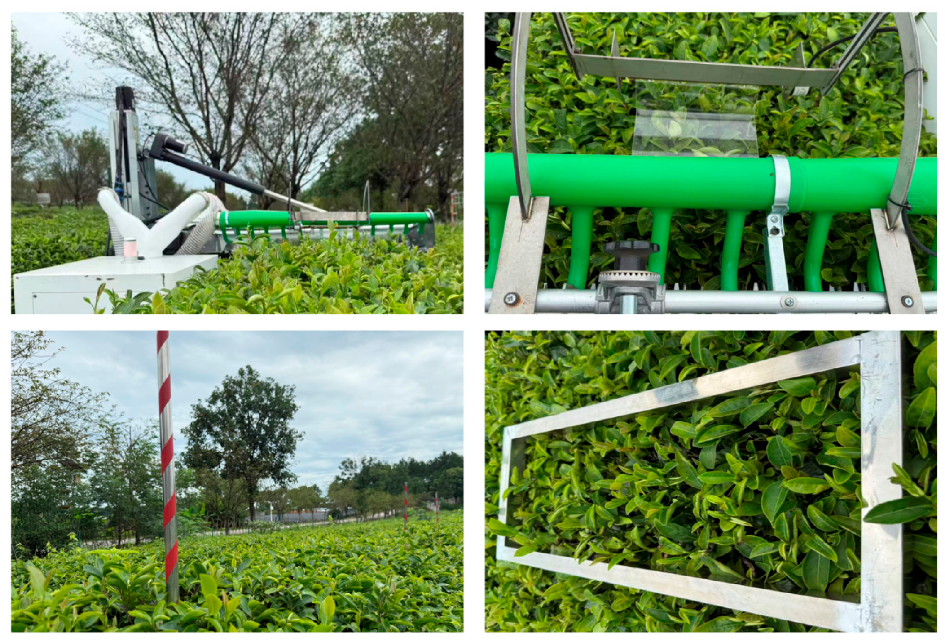
Figure 17.
Field operational performance and closed-loop validation of the adaptive profiling architecture: (a) raw heterogeneous perception signals collected by on-machine sensors during field operations; (b) closed-loop tracking responses and error dynamics generated via Processor-in-the-Loop validation using the actual on-machine sensor logs.
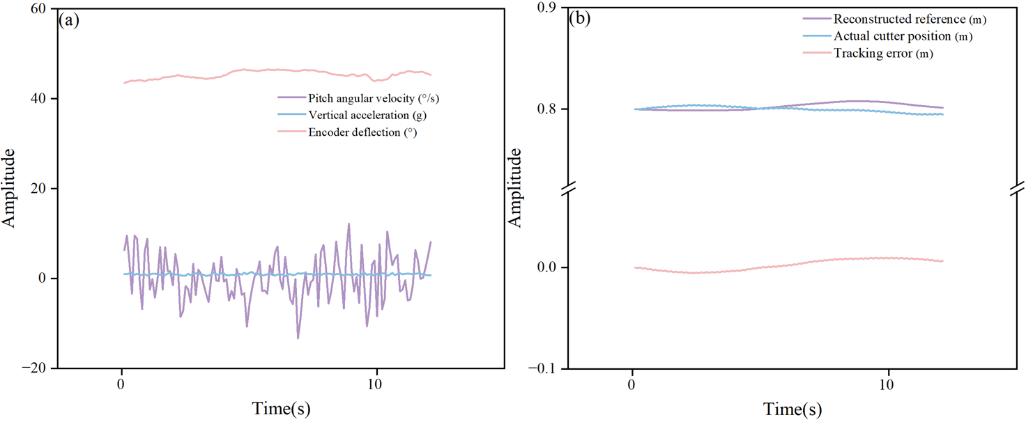
Table 6.
Field-test conditions and tea-garden agronomic parameters.
Table 7.
Descriptive under variable operating conditions (N = 5 per algorithm per scenario).
3.5.2. Algorithm Computational Overhead and Timing Feasibility
Multisource filtering and nonsingular sliding-mode control inherently increase computational demand. To assess timing feasibility on the actual vehicle-mounted controller, Processor-in-the-Loop tests were conducted for the three control architectures using a vehicle-mounted controller over 2000 independent control steps on the vehicle-mounted main controller (STM32 microcontroller (STMicroelectronics, Geneva, Switzerland), 32-bit ARM Cortex-M7 core at 400 MHz with double-precision FPU and 1 MB RAM, communicating with the HDS6A IMU and servo drive via 500 kbps CAN bus). Using the hardware DWT cycle counter, the per-step timing measurement encompasses raw sensor frame parsing, inverse-kinematics mapping (Equations (1)–(4)), FIFO delay alignment, 40-sample Huber IRLS optimization and VB-STF gain update (Equations (8)–(14)), and TD-based feedforward and anti-windup NFTSMC law computation (Equations (15)–(25)), excluding external CAN bus transmission waiting time. Despite the additional computational complexity introduced by VB noise adaptation and Huber-window optimization, the proposed ARMHE-NFTSMC architecture remained below the nominal control-period requirement. The baseline KF-PID algorithm required an average execution time of 0.18 ms. For the proposed ARMHE-NFTSMC, the average execution time was 0.88 ms. Under composite disturbance conditions, its worst-case latency was recorded at 2.34 ms, with a timing jitter of 0.22 ms (Table 8). This maximum single-step execution time remains well below the 5.0 ms control period at 200 Hz, supporting computational feasibility for real-time deployment.
3.5.3. Field Agronomic Performance and Harvesting Performance
To evaluate the agronomic efficacy of the profiling control architectures, a field validation framework was implemented as a compound-scenario comparison across two distinct operating conditions: a Base Scenario (gentle slope, 0.4 m/s travel speed, 1858 shoots/m2) and a Challenging Scenario (moderate slope, 0.8 m/s travel speed, 1350 shoots/m2). To prevent spatial confounding effects, a completely randomized design (CRD) within each scenario was utilized for the field layout. For each scenario, the three control algorithms were evaluated across five 5 m measurement areas (N = 5 per algorithm per scenario, yielding 30 samples overall), spatially separated by a 2 m non-measurement buffer zone to allow chassis and actuator states to stabilize before each measurement phase. Because the allocation of the three control algorithms across the homogeneous plots and their execution order were completely randomized, one-way ANOVA (SPSS, 26.0, IBM Corp., Armonk, NY, USA) was applied separately to each scenario using Yij = μ + Ci + εij, with measurement area as the experimental unit and no block term. The masses of cut fresh leaves (W1), uncollected leaves (W2), and uncut fresh shoots (W3) were recorded to calculate the loss rate (R1) and missed-plucking rate (R2). The descriptive and inferential statistics are summarized in Table 7, and the comprehensive raw data for all 30 measurement areas are provided. Actual cutting depth was independently checked after harvesting at 10 equidistant points per plot using a reference leveling frame and a steel rule, as the vertical height difference between the unplucked canopy top plane and the cut surface. This measurement was separate from the encoder/IMU feedback and PIL reconstruction.
Table 8.
Execution time statistics of the control algorithms based on vehicle-mounted controller Processor-in-the-Loop validation.
One-way analysis of variance (ANOVA) followed by Tukey’s HSD post hoc test revealed a statistically significant main effect of the control architecture on both the loss rate and the missed-plucking rate. For the loss rate, significant effects were observed under the Base Scenario (F(2,12) = 44.19, p < 0.001, ) and the Challenging Scenario (F(2,12) = 123.45, p < 0.001, ). Similarly, for the missed-plucking rate, significant effects were found under the Base Scenario (F(2,12) = 109.12, p < 0.001, ) and the Challenging Scenario (F(2,12) = 208.35, p < 0.001, ).
Under the Base Scenario, the KF-PID algorithm exhibited a mean loss rate of 0.70% and a mean missed-plucking rate of 0.99%. Because error-driven integral regulation is susceptible to chassis-pitch disturbances, it produced a measurable response lag in the cutter actuator. The SMHE-SMC algorithm improved nonlinear tracking, reducing the mean missed-plucking rate to 0.57%; however, hard sign-function switching induced high-frequency electromechanical chattering at the cutter, yielding a mean loss rate of 0.44%. In contrast, the ARMHE-NFTSMC reduced disturbance transmission to the end-effector, resulting in the lowest mean loss rate (0.15%) and missed-plucking rate (0.20%).
The performance divergence among the algorithms was magnified under the Challenging Scenario. Given that slope, travel speed, and shoot density varied simultaneously between the two scenarios, the observed performance differences represent the cumulative effect of these concurrent variables. Under these compounded disturbances, the KF-PID algorithm showed degraded tracking (mean R2 = 2.52%, mean R1 = 1.84%), as uncompensated phase lag and actuator overshoot caused cutter oscillations. The SMHE-SMC algorithm also experienced deterioration (mean R2 = 1.52%, mean R1 = 1.30%) due to actuator torque saturation exacerbating windup-related oscillations. Conversely, by utilizing pitch-rate feedforward to anticipate spatial displacement and anti-windup auxiliary dynamics to compensate for actuator saturation, the proposed ARMHE-NFTSMC restricted the mean missed-plucking rate to 0.46% and the mean loss rate to 0.43%. The observed effect sizes () indicate that the proposed architecture reduces missed plucking and collection loss under the tested field conditions.
4. Discussion
4.1. Global Mapping and Spatiotemporal Perception in Unstructured Terrain
The first two findings are linked: inverse-kinematics mapping establishes a global canopy-elevation reference by separating chassis posture from local canopy observations, and the ARMHE preserves this reference under impulsive and time-varying noise. Noncontact modalities, such as LiDAR and RGB-D cameras, have been applied to map crop height, density, and 3D pose in agricultural scenarios like grain harvesting [21,22] and orchard navigation [23,24,25]. However, in unstructured hilly tea gardens, a fixed 2D LiDAR [26] or vision system can be affected by the vibrations of the crawler chassis, which may introduce deviations in localized point clouds. Similarly, current ultrasonic profiling schemes can experience acoustic scattering and often rely on linear Gaussian filters, such as recursive average filtering [27]. These linear filters may yield temporal phase lag and biased reference trajectories when processing non-Gaussian transient impulses generated by rigid branch impacts [28]. The proposed architecture addresses this by decoupling the chassis inertial posture from local terrain observations via a global inverse-kinematics mapping model, which reduces the influence of chassis pitching on the elevation reference. Compared to methods relying primarily on spatial-domain geometric fitting (e.g., RANSAC) [26], the robust ARMHE processes noise spatiotemporally. The Huber penalty is utilized to suppress high-amplitude non-Gaussian outliers, while the VB-STF adjusts the temporal bandwidth. In the impact-disturbance simulation, this combination reduced the maximum absolute deviation by 69.0% relative to KF while maintaining the dynamic response.
4.2. Feedforward Anti-Windup Control and Tracking Improvement
Precision profiling is constrained by the interaction between large mechanical inertia and actuator torque limits (±10 N·m). Linear controllers, such as incremental PID, can experience integral windup during abrupt posture changes, requiring stabilization periods (e.g., 1.6–2.2 s) to re-level the header [27,29]. Alternatively, applying unmodified SMC under hardware constraints may induce high-frequency electromechanical chattering [30]. During actuator saturation, this chattering can lead the closed-loop tracking curves to diverge from the target manifold [31,32]. The proposed ARMHE-NFTSMC is designed to mitigate this divergence. By utilizing a fractional-order nonsingular fast terminal sliding surface with a continuous boundary layer, high-frequency command oscillations are smoothed. Additionally, the integrated anti-windup auxiliary dynamics feed the saturation residual back into the error manifold. This approach limits controller-state accumulation during terrain steps, with conditional dissipation and ideal sliding-phase convergence analyzed in Section 2.4.5, thereby reducing the tracking divergence observed in conventional PID and standard SMC architectures. The 41.1% reduction in tracking RMS relative to KF-PID under S4 is therefore interpreted as the combined effect of faster posture compensation, saturation-state correction, and continuous command smoothing, rather than as the contribution of a single module.
4.3. Field Performance, Validation Limits, and Future Work
At the agronomic level, lower mean missed-plucking and collection loss rates were observed with ARMHE-NFTSMC under the tested conditions. However, because R1 and R2 only quantify harvesting completeness and collection efficiency rather than direct leaf-quality attributes (such as the intact shoot rate, shoot length uniformity, or old-leaf impurity ratio), the current field conclusions are strictly limited to reducing missed cutting and leaf loss under the tested slope (≤8∘) and speed (0.4−0.8 m/s) conditions. Several limitations remain to be addressed in future work:
- (1)
- Multi-degree-of-freedom flexible cutters for irregular canopies: Rigid contact plates and linear reciprocating cutters present geometric limitations on naturally grown, curved canopies. Future work will investigate multi-degree-of-freedom flexible cutters to overcome the geometric constraints of current mechanisms.
- (2)
- Multimodal spatiotemporal fusion for comprehensive perception: Integrating near-field contact feedback with lightweight 3D LiDAR or UAV-based multispectral point clouds [33,34,35,36] could help construct a more comprehensive global canopy geometry. This multimodal spatiotemporal fusion will potentially expand the operational applicability of intelligent harvesting machinery.
- (3)
- Extended environmental validation: While actual field evaluations across two scenarios demonstrated statistically significant improvements, future work will focus on expanding long-term multi-site validation across diverse terrains and tea varieties to further verify the system’s global adaptability.
- (4)
- Single-factor and factorial field evaluations: In the current field evaluations, the Base and Challenging scenarios were evaluated as a compound-scenario comparison, characterized by simultaneous variations in slope, travel speed, and shoot density. Consequently, the specific contribution of each individual factor to the observed performance variance was not isolated. Future research will employ single-factor and factorial experimental designs to quantitatively decouple the respective influences of travel speed, terrain slope, and canopy density on profiling precision.
5. Conclusions
This study shows that dynamic profiling in hilly tea gardens benefits from coordinating global kinematic mapping, spatiotemporal perception reconstruction, and saturation-aware control. Global kinematic mapping decouples chassis-posture changes from local canopy observations and provides a common reference for constant-depth profiling. Spatiotemporal reconstruction combines robust amplitude-domain outlier suppression with adaptive temporal bandwidth to reject impulsive disturbances without sacrificing rapid tracking. This perception layer therefore stabilizes the canopy-elevation reference under mixed vibration, impact, and terrain-change disturbances. At the actuator level, pitch-rate feedforward, continuous boundary-layer control, and anti-windup dynamics jointly mitigate lag, chattering, and saturation-induced error accumulation. Their coordinated action improves closed-loop profiling under composite disturbances while respecting the motor torque constraint. Furthermore, the structured component-wise ablation analyses isolated the effects of the core modules, confirming their respective roles in mitigating spatial observation drift, reducing temporal phase lag, and maintaining actuator state stability under structural limits. Field harvesting trials across 30 plots showed that, within the tested conditions of gentle-to-moderate slopes (≤8∘), travel speeds of 0.4−0.8 m/s, and shoot densities of 1350−1858 shoots/m2, the proposed architecture achieved lower missed-plucking (0.20−0.46%) and collection loss (0.15−0.43%) rates than the KF-PID and SMHE-SMC benchmarks. Combined with onboard Processor-in-the-Loop timing verification (worst-case latency of 2.34 ms within a 5.0 ms cycle), these results confirm the computational and operational feasibility of the control scheme for bulk tea profiling, while direct evaluations of shoot integrity and multi-site adaptability remain for future investigation.
Author Contributions
Conceptualization, L.W. and H.L.; methodology, H.L. and C.Y.; software, Y.W. and C.D.; validation, Y.W. and C.Y.; formal analysis, Y.W. and C.D.; investigation, H.L. and C.Y.; resources, L.W., S.S. and C.Y.; data curation, H.L. and Y.W.; writing—original draft preparation, H.L.; writing—review and editing, L.W.; visualization, Y.W. and C.D.; supervision, C.Y.; project administration, S.S. and C.Y.; funding acquisition, L.W., S.S. and C.Y. All authors have read and agreed to the published version of the manuscript.
Funding
This work was partially supported by Jiangxi Province Agricultural Machinery Equipment R&D, Manufacturing, and Promotion-Application Integration Pilot Project (YCTY202408), Basic Research and Talent Cultivation Project of Jiangxi Academy of Agricultural Sciences (JXSNKYJCRC202450), and Jiangxi Collaborative Innovation Project for Modern Agricultural Scientific Research (JXXTCX202603).
Institutional Review Board Statement
Not applicable.
Data Availability Statement
Data are available at https://github.com/li-have/teamachines (accessed on 5 September 2026).
Acknowledgments
Thanks to Fu Hao and Zheng Lianyou for their assistance during the research process. The authors did not use AI-assisted technologies for experimental design, article structure, or data analysis; DeepSeek-V2 was used only for grammar checking and readability improvement. After using this tool, the authors reviewed and edited the content as needed and take full responsibility for the content of the article.
Conflicts of Interest
The authors declare no conflicts of interest.
Abbreviations
The following abbreviations are used in this manuscript:
| AEKF | Adaptive Extended Kalman Filter |
| ANOVA | Analysis of Variance |
| ARMHE | Adaptive Robust Moving Horizon Estimation |
| AW | Anti-Windup |
| BL | Boundary Layer |
| CM | Complete Model |
| FF | Feedforward |
| FPID | Fuzzy Proportional-Integral-Derivative |
| HSD | Honestly Significant Difference |
| IK | Inverse Kinematics |
| IMU | Inertial Measurement Unit |
| KF | Kalman Filter |
| LiDAR | Light Detection and Ranging |
| MAD | Median Absolute Deviation |
| MAX | Maximum Absolute Deviation |
| MHE | Moving Horizon Estimation |
| NFTSMC | Nonsingular Fast Terminal Sliding Mode Control |
| PID | Proportional-Integral-Derivative |
| PIL | Processor-in-the-Loop |
| PSD | Power Spectral Density |
| RANSAC | Random Sample Consensus |
| RGB-D | Red, Green, Blue, and Depth |
| RMS | Root Mean Square |
| SMC | Sliding Mode Control |
| SMHE | Standard Moving Horizon Estimation |
| STF | Strong Tracking Filter |
| TD | Tracking Differentiator |
| TV | Total Variation |
| UAV | Unmanned Aerial Vehicle |
| UUB | Uniform Ultimate Boundedness |
| Var | Variance |
| VB | Variational Bayesian |
Appendix A
Table A1.
Comprehensive raw data of field plucking performance across 30 measurement areas under different operating scenarios.
Table A2.
Physical, perception, and controller parameters.
| Algorithm A1. Per-sample implementation outline |
| 1. Correct sensor biases, update the kinematic mapping, and apply FIFO alignment (Equations (1)–(4)). 2. Update the observation window and perform five Huber IRLS iterations (Equations (8) and (9)). 3. Update the robust variance, VB posterior, STF index and clipped tracking gain; update xr (Equations (10)–(14)). 4. Apply d0 once, calculate e and ec = e − ξ, and form the sliding variable (Equations (6), (18) and (19)). 5. Update the TD, feedforward, feedback and bounded adaptive compensation; include ucomp = Kcξ. 6. Saturate uraw, calculate Δu = uout − uraw, and update ξk+1 = ξk + Ts(−Kξξk + b0Δuk). |
References
- Li, Y.; Wu, S.; He, L.; Tong, J.; Zhao, R.; Jia, J.; Chen, J.; Wu, C. Development and field evaluation of a robotic harvesting system for plucking high-quality tea. Comput. Electron. Agric. 2023, 206, 107659. [Google Scholar] [CrossRef] [Scilit]
- Abhiram, G. The evolution of tea harvesting: A comprehensive review of machinery and technological advancements. J. Biosyst. Eng. 2024, 49, 346–367. [Google Scholar] [CrossRef] [Scilit]
- Wang, Q.; Meng, Z.; Wen, C.; Qin, W.; Wang, F.; Zhang, A.; Zhao, C.; Yin, Y. Grain combine harvester header profiling control system development and testing. Comput. Electron. Agric. 2024, 223, 109082. [Google Scholar] [CrossRef] [Scilit]
- Han, Y.; Xiao, H.R.; Song, Z.Y.; Chen, Q.M.; Ding, W.Q.; Mei, S. Design and experiments of 4CJ-1200 self-propelled tea plucking machine. Int. J. Agric. Biol. Eng. 2021, 14, 75–84. [Google Scholar] [CrossRef] [Scilit]
- He, Y.; Zhou, J.; Sun, J.; Jia, H.; Gemechu, T.T. Traveling control method adapted to different paddy ground conditions with feedforward compensation for crawler combine harvester based on online tracking error prediction. Comput. Electron. Agric. 2024, 220, 108853. [Google Scholar] [CrossRef] [Scilit]
- He, Y.; Zhou, J.; Sun, J.; Jia, H.; Liang, Z.; Awuah, E. An adaptive control system for path tracking of crawler combine harvester based on paddy ground conditions identification. Comput. Electron. Agric. 2023, 210, 107948. [Google Scholar] [CrossRef] [Scilit]
- Han, Y.; Song, Z. Tea canopy detection algorithm based on multi-sensor data fusion. Smart Agric. Technol. 2025, 12, 101497. [Google Scholar] [CrossRef] [Scilit]
- Bai, Y.; Zhang, B.; Xu, N.; Zhou, J.; Shi, J.; Diao, Z. Vision-based navigation and guidance for agricultural autonomous vehicles and robots: A review. Comput. Electron. Agric. 2023, 205, 107584. [Google Scholar] [CrossRef] [Scilit]
- Yi, X.; Zheng, Z.; Wu, P.; Gadekallu, T.; Fang, K. Multi-scale tea bud grading detection in complex tea garden scenes based on a GenAI training framework. Comput. Electron. Agric. 2025, 239, 111032. [Google Scholar] [CrossRef] [Scilit]
- Zhang, X.; Huang, Y.; Wang, P.; Liang, L.; Cheng, Y.; Liu, P.; Sun, L. Vibration characteristics of a terrain-adaptive agricultural chassis for hilly and mountainous terrain. Biosyst. Eng. 2026, 261, 104338. [Google Scholar] [CrossRef] [Scilit]
- Barač, Ž.; Radočaj, D.; Plaščak, I.; Jurišić, M.; Zimmer, D. Prediction of noise levels according to some exploitation parameters of an agricultural tractor: A machine learning approach. AgriEngineering 2024, 6, 995–1007. [Google Scholar] [CrossRef] [Scilit]
- Khodarahmi, M.; Maihami, V. A review on Kalman filter models. Arch. Comput. Methods Eng. 2023, 30, 727–747. [Google Scholar] [CrossRef] [Scilit]
- Zhang, Z.; Kayacan, E.; Thompson, B.; Chowdhary, G. High precision control and deep learning-based corn stand counting algorithms for agricultural robot. Auton. Robot 2020, 44, 1289–1302. [Google Scholar] [CrossRef] [Scilit]
- Deng, W.; Yao, J. Extended-state-observer-based adaptive control of electro-hydraulic servomechanisms without velocity measurement. IEEE/ASME Trans. Mechatron. 2019, 25, 1151–1161. [Google Scholar] [CrossRef] [Scilit]
- Somefun, O.A.; Akingbade, K.; Dahunsi, F. The dilemma of PID tuning. Annu. Rev. Control 2021, 52, 65–74. [Google Scholar] [CrossRef] [Scilit]
- Mohindru, P. Review on PID, fuzzy and hybrid fuzzy PID controllers for controlling non-linear dynamic behaviour of chemical plants. Artif. Intell. Rev. 2024, 57, 97. [Google Scholar] [CrossRef] [Scilit]
- Han, Y.; Xiao, H.R.; Song, Z.Y.; Ding, W.Q. Design and evaluation of tea-plucking machine for improving quality of tea. Appl. Eng. Agric. 2019, 35, 979–986. [Google Scholar] [CrossRef] [Scilit]
- Utkin, V.; Poznyak, A.; Orlov, Y.; Polyakov, A. Conventional and high order sliding mode control. J. Frankl. Inst. 2020, 357, 10244–10261. [Google Scholar] [CrossRef] [Scilit]
- Shao, K.; Zheng, J.; Wang, H.; Xu, F.; Liang, B. Recursive sliding mode control with adaptive disturbance observer for a linear motor positioner. Mech. Syst. Signal Process. 2021, 146, 107014. [Google Scholar] [CrossRef] [Scilit]
- Zou, M.; Fang, P.; Hou, Y.; Peng, H. Investigation on multiple-frequency synchronization experiment of vibration system with dual-rotor actuation. Mech. Syst. Signal Process. 2022, 164, 108261. [Google Scholar] [CrossRef] [Scilit]
- Blanquart, J.E.; Sirignano, E.; Lenaerts, B.; Saeys, W. Online crop height and density estimation in grain fields using LiDAR. Biosyst. Eng. 2020, 198, 1–14. [Google Scholar] [CrossRef] [Scilit]
- Lee, J.; Ohata, M.; Itoh, H.; Morimoto, E. LiDAR–camera fusion for 3D fruit counting and density mapping in horizontal trellis orchards. J. Robot. Mechatron. 2026, 38, 449–459. [Google Scholar] [CrossRef] [Scilit]
- Eizentals, P.; Oka, K. 3D pose estimation of green pepper fruit for automated harvesting. Comput. Electron. Agric. 2016, 128, 127–140. [Google Scholar] [CrossRef] [Scilit]
- Liu, T.; Kang, H.; Chen, C. ORB-Livox: A real-time dynamic system for fruit detection and localization. Comput. Electron. Agric. 2023, 209, 107834. [Google Scholar] [CrossRef] [Scilit]
- Mahmud, M.S.; Zahid, A.; He, L.; Choi, D.; Krawczyk, G.; Zhu, H.; Heinemann, P. Development of a LiDAR-guided section-based tree canopy density measurement system for precision spray applications. Comput. Electron. Agric. 2021, 182, 106053. [Google Scholar] [CrossRef] [Scilit]
- Huan, X.; Wu, M.; Bian, X.; Jia, J.; Kang, C.; Wu, C.; Zhao, R.; Chen, J. Design and experiment of ordinary tea profiling harvesting device based on light detection and ranging perception. Agriculture 2024, 14, 1147. [Google Scholar] [CrossRef] [Scilit]
- Zhang, D.; Zhang, R.; Chen, L.; Zhang, L.; Yi, T.; Feng, Q. Adaptive tracking and cutting control system for tea canopy: Design and experimental evaluation. Agriculture 2025, 15, 557. [Google Scholar] [CrossRef] [Scilit]
- Wang, D.; Struik, P.C.; Liang, L.; Liu, X. Enhancing crop growth forecasting by incorporating estimated uncertainties for time-series hyperspectral data and crop model GECROS simulations into ensemble Kalman filter. Comput. Electron. Agric. 2025, 239, 111057. [Google Scholar] [CrossRef] [Scilit]
- Huang, X.; Wang, Z.; Wang, X.; Shi, Y.; Huang, X.; Wang, B.; Lin, L.; Wang, Y. Adaptive fuzzy coordinated control of orchard mowing robots using cutter torque-feedforward–SMC and chassis ICOA–Smith–RBF–PID strategies. Comput. Electron. Agric. 2026, 243, 111320. [Google Scholar] [CrossRef] [Scilit]
- Shao, K.; Zheng, J.; Huang, K.; Wang, H.; Man, Z.; Fu, M. Finite-time control of a linear motor positioner using adaptive recursive terminal sliding mode. IEEE Trans. Ind. Electron. 2019, 67, 6659–6668. [Google Scholar] [CrossRef] [Scilit]
- Luckert, F.; Dempewolf, K.H.; Mertens, A. Control of a dual-stage positioning system consisting of two permanent magnet linear motors for high-precision applications. In Proceedings of the 2023 14th International Symposium on Linear Drives for Industry Applications (LDIA); IEEE: Piscataway, NJ, USA, 2023; pp. 1–5. [Google Scholar]
- Zou, M.; Wang, Y.; Zhu, W.; Wang, Y.; Xie, D.; Kong, C.; Tang, S. Counter-rotating synchronization theory and experiment of tri-rotor actuated with dual-frequency considering adaptive global sliding mode control strategy. Mech. Syst. Signal Process. 2025, 223, 111820. [Google Scholar] [CrossRef] [Scilit]
- Gené-Mola, J.; Gregorio, E.; Cheein, F.A.; Guevara, J.; Llorens, J.; Sanz-Cortiella, R.; Escolà, A.; Rosell-Polo, J.R. Fruit detection, yield prediction and canopy geometric characterization using LiDAR with forced air flow. Comput. Electron. Agric. 2020, 168, 105121. [Google Scholar] [CrossRef] [Scilit]
- Maimaitijiang, M.; Sagan, V.; Sidike, P.; Hartling, S.; Esposito, F.; Fritschi, F.B. Soybean yield prediction from UAV using multimodal data fusion and deep learning. Remote Sens. Environ. 2020, 237, 111599. [Google Scholar] [CrossRef] [Scilit]
- de Sá Leitão, D.A.H.; Sharma, A.K.; Singh, A.; Sharma, L.K. Yield and plant height predictions of irrigated maize through unmanned aerial vehicle in North Florida. Comput. Electron. Agric. 2023, 215, 108374. [Google Scholar] [CrossRef] [Scilit]
- Nidamanuri, R.R.; Jayakumari, R.; Ramiya, A.M.; Astor, T.; Wachendorf, M.; Buerkert, A. High-resolution multispectral imagery and LiDAR point cloud fusion for the discrimination and biophysical characterisation of vegetable crops at different levels of nitrogen. Biosyst. Eng. 2022, 222, 177–195. [Google Scholar] [CrossRef] [Scilit]
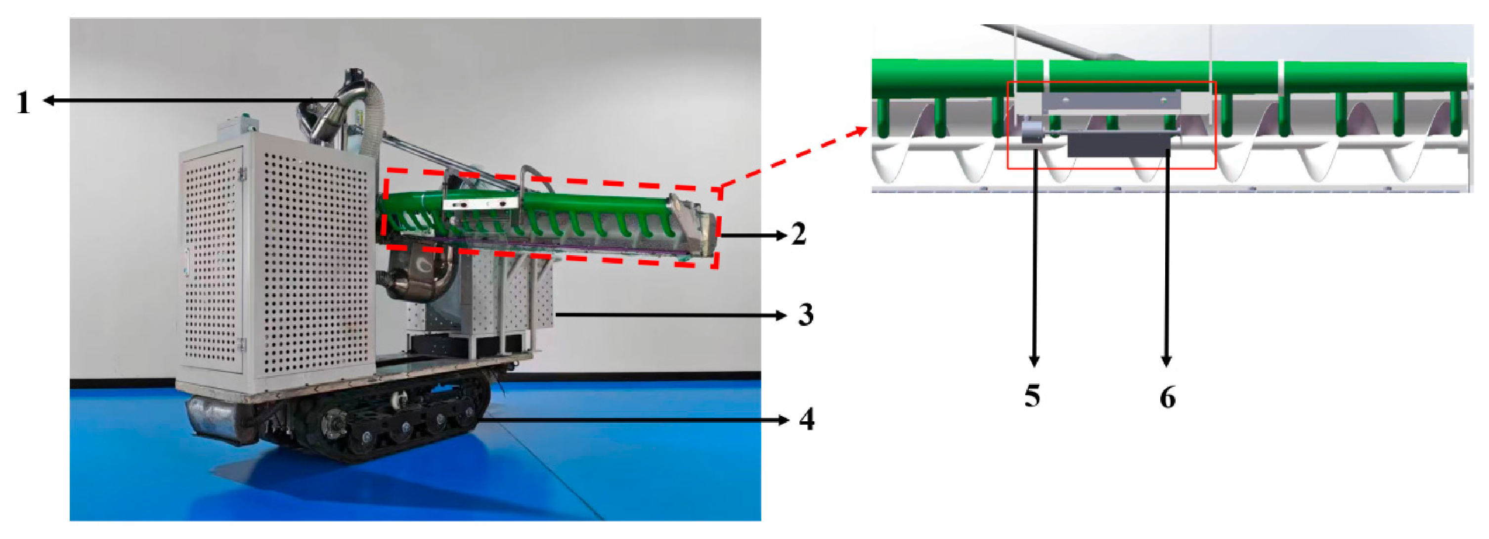
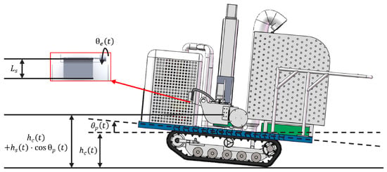
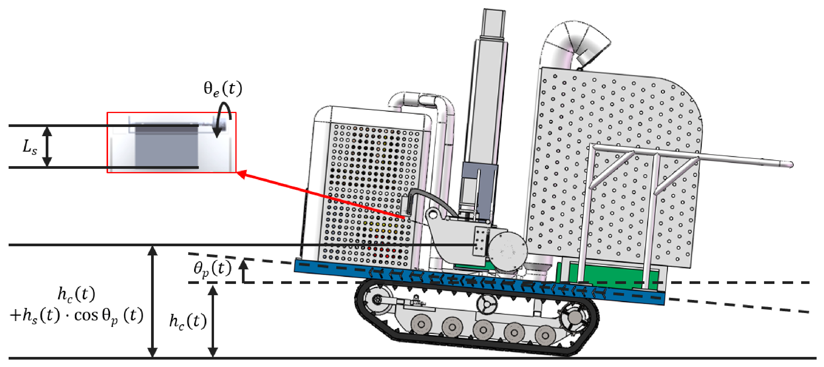
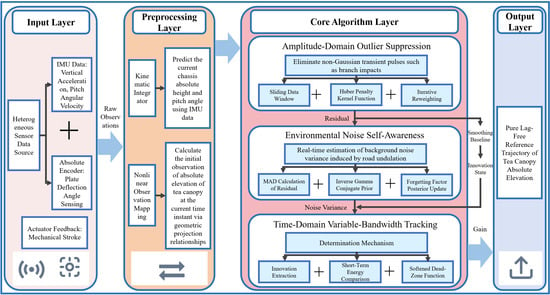
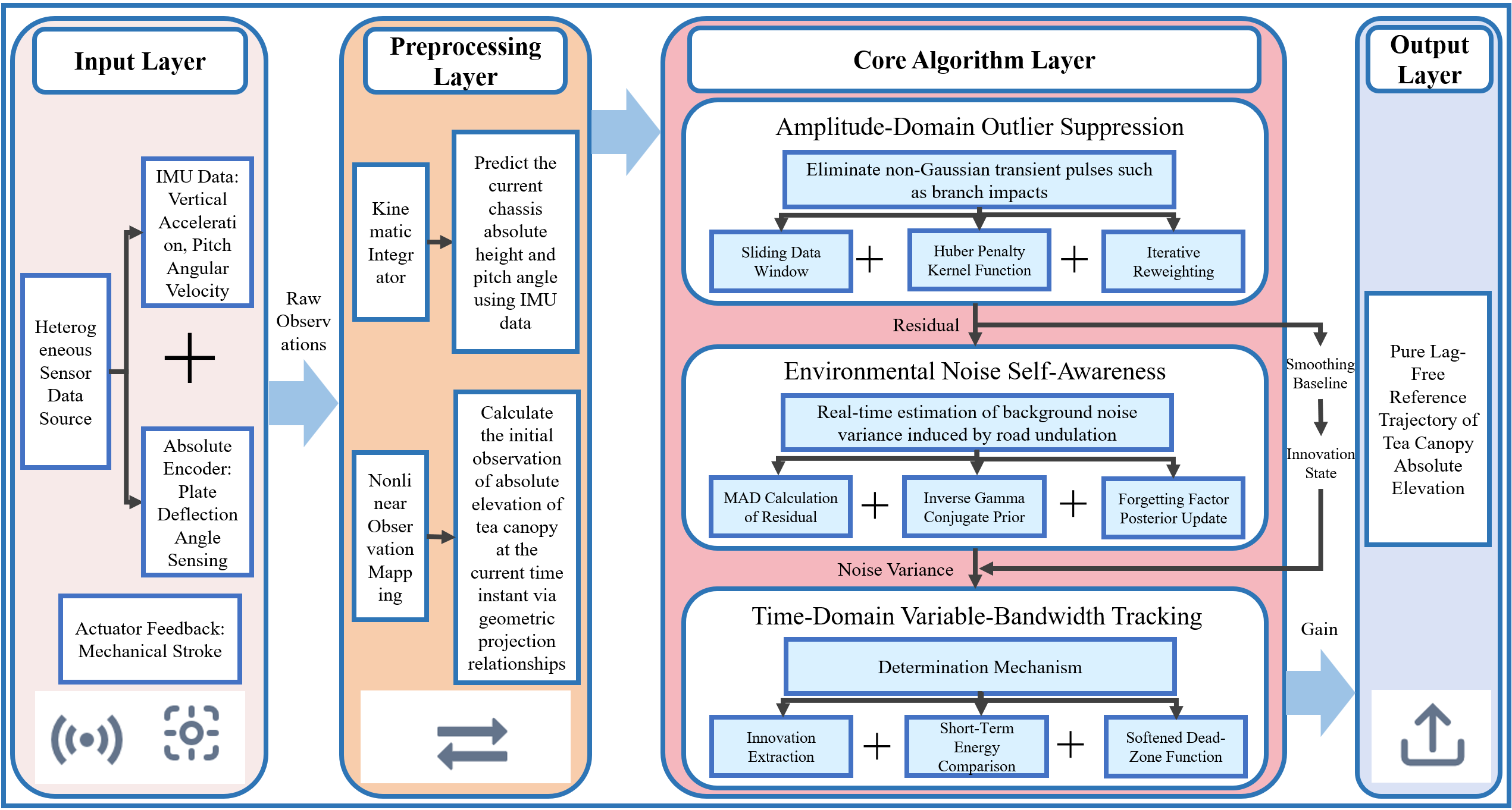
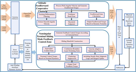
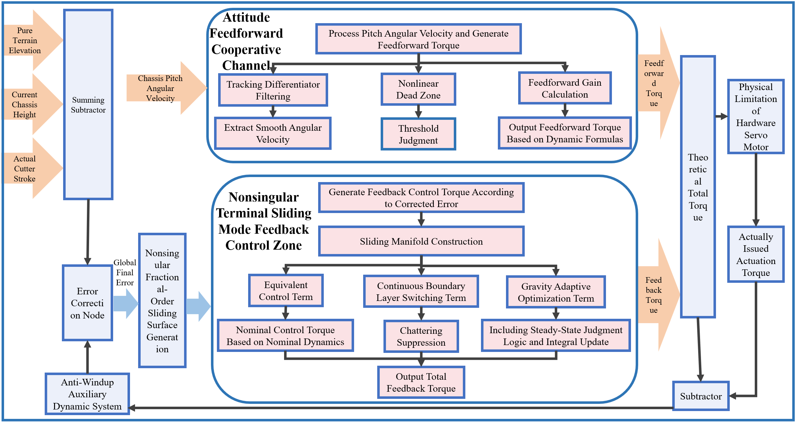
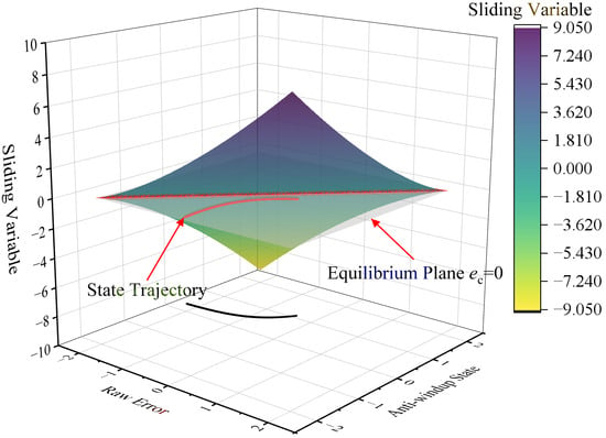
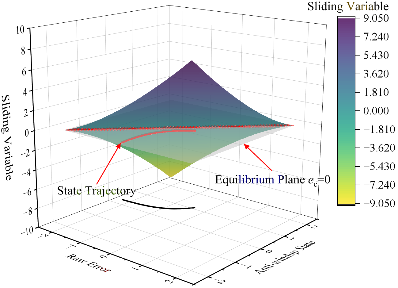
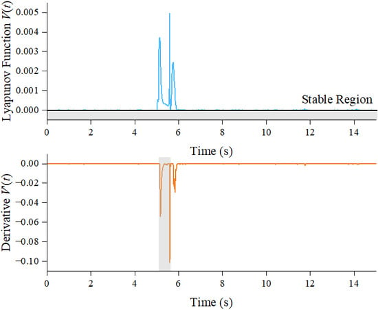
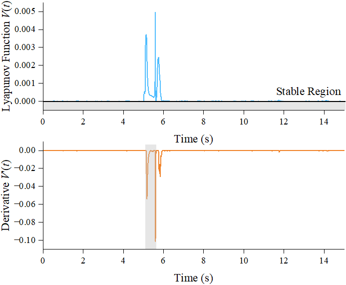
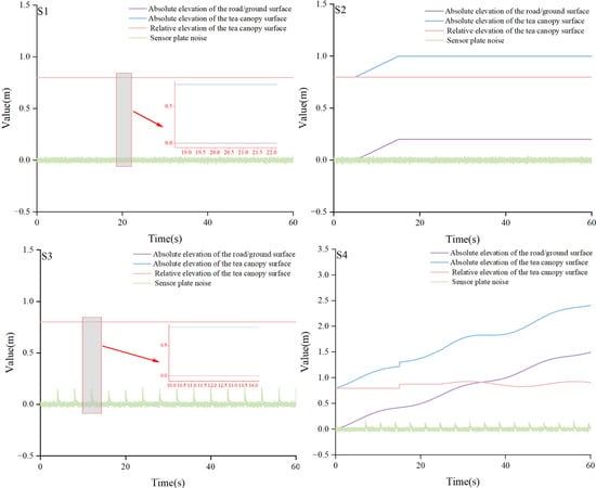
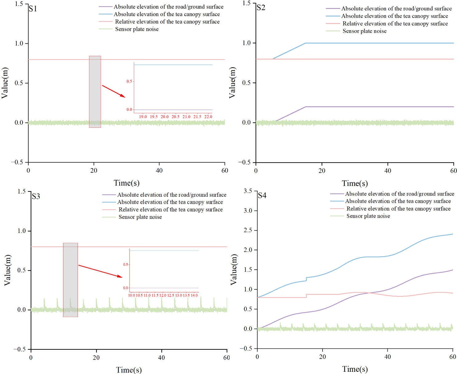
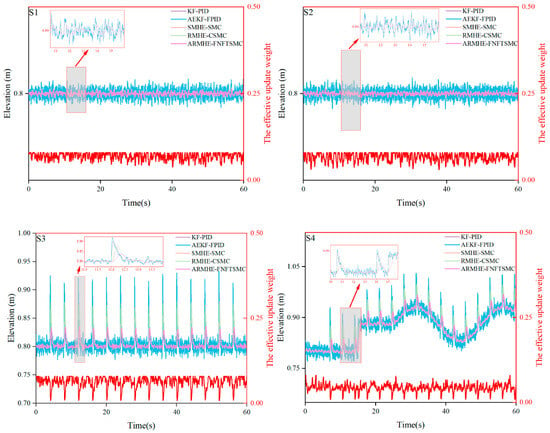
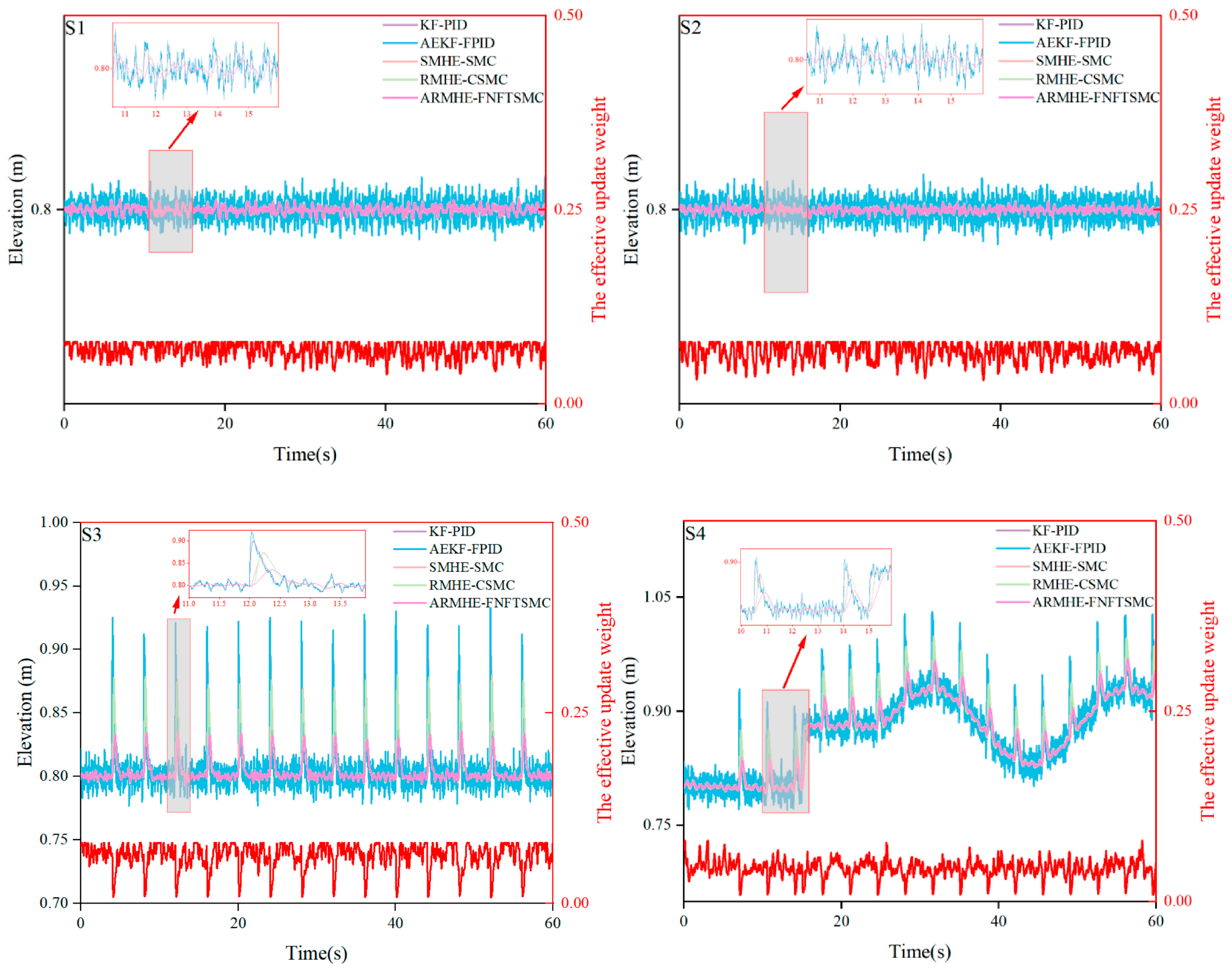
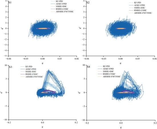
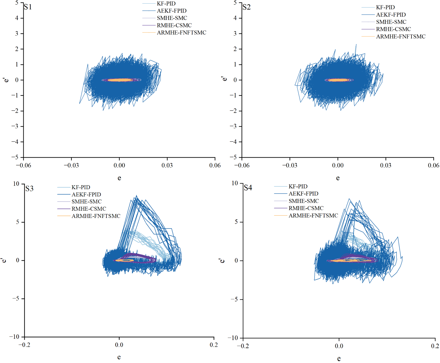
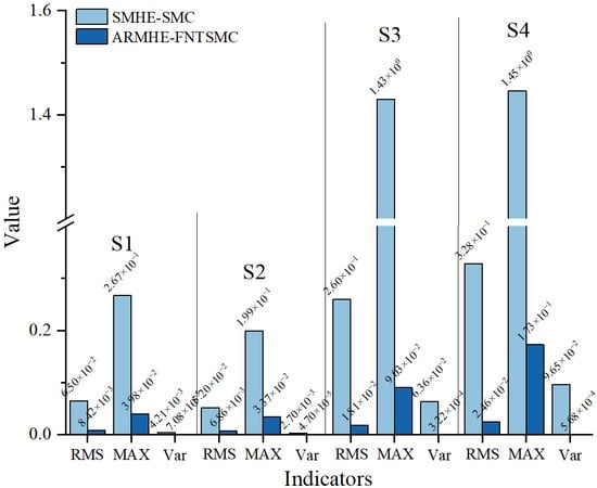
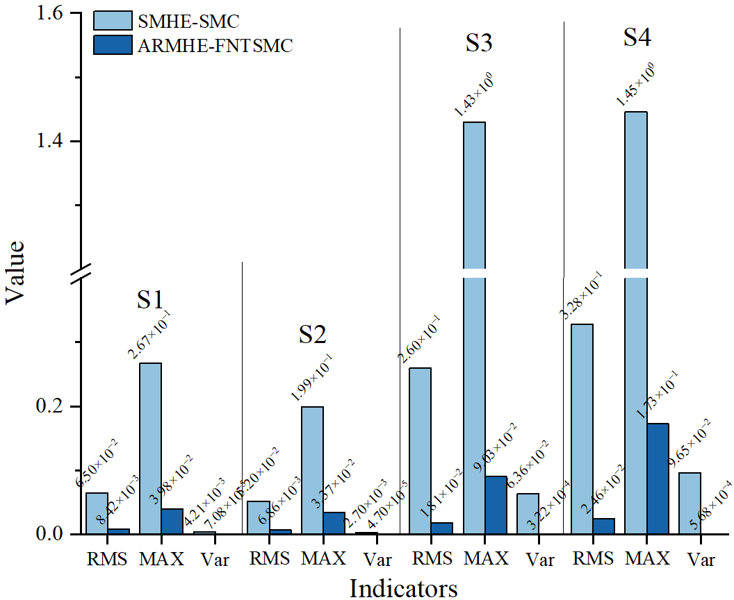
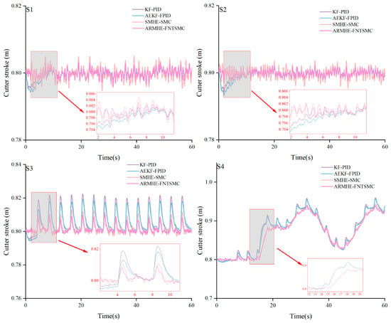
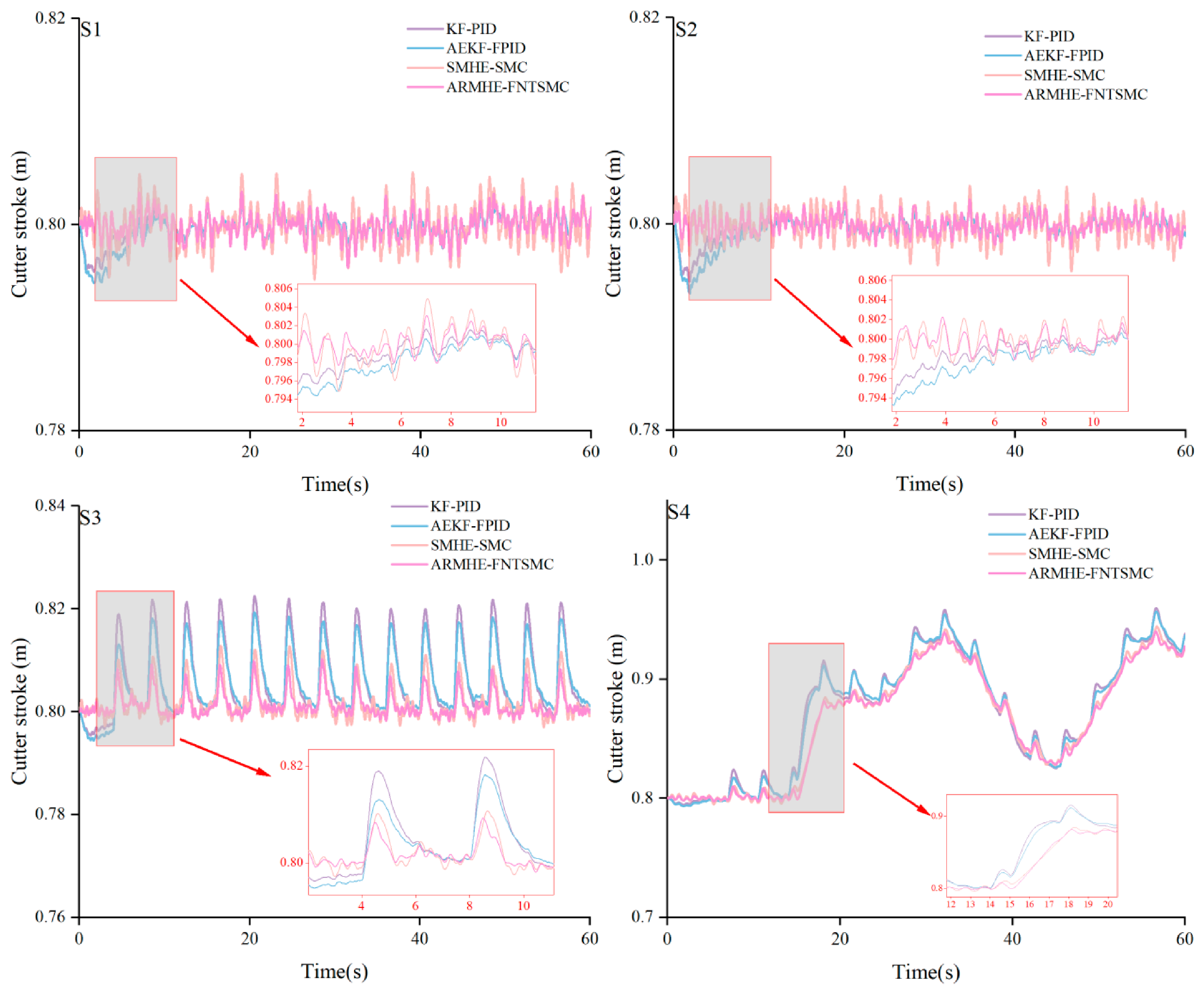
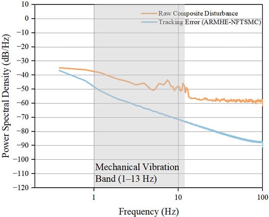
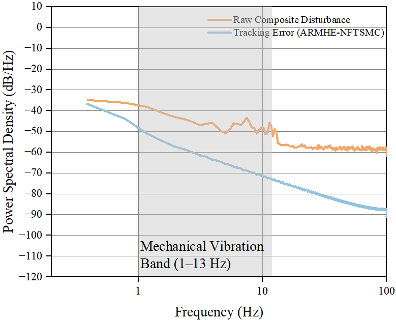
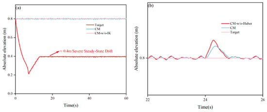
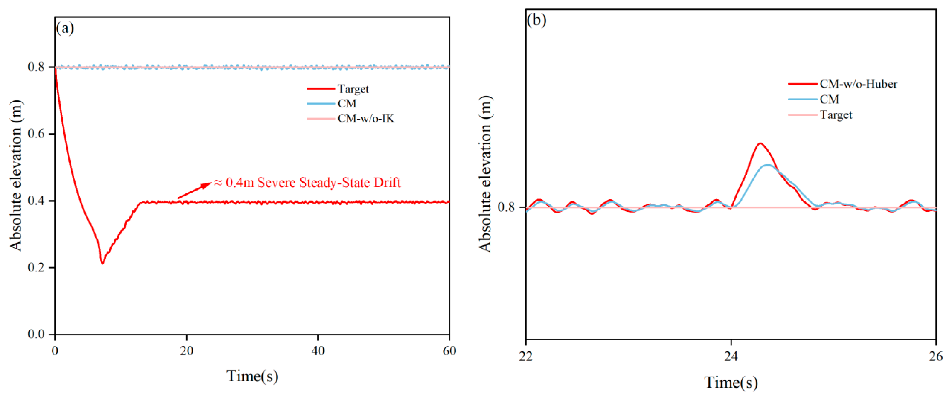
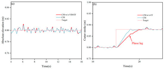
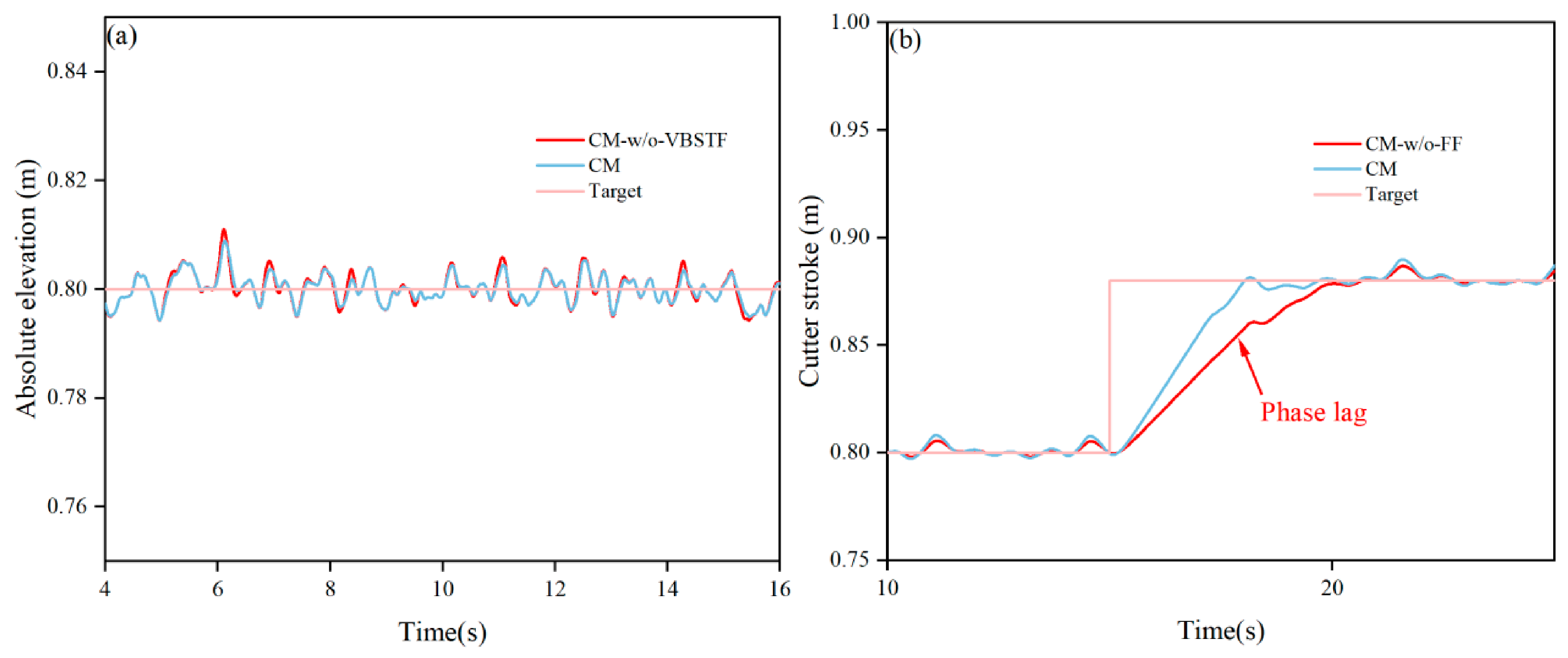
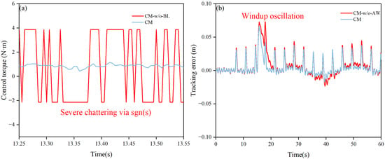
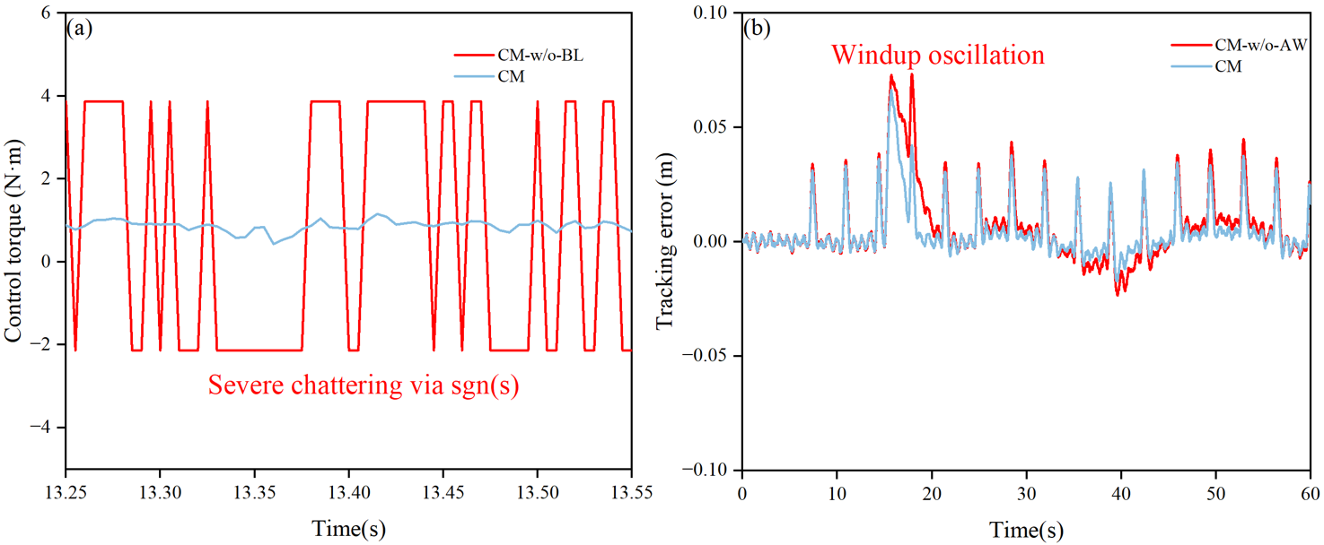

Disclaimer/Publisher’s Note: The statements, opinions and data contained in all publications are solely those of the individual author(s) and contributor(s) and not of MDPI and/or the editor(s). MDPI and/or the editor(s) disclaim responsibility for any injury to people or property resulting from any ideas, methods, instructions or products referred to in the content. |
© 2026 by the authors. Licensee MDPI, Basel, Switzerland. This article is an open access article distributed under the terms and conditions of the Creative Commons Attribution (CC BY) license.