


Abstract
Korea produces comparatively less summer-cultivated paprika from August to September due to unfavorable environmental circumstances, particularly high temperatures that begin in late June. As a result of this, managing a greenhouse climate well during the hot season is essential to boosting paprika production and ensuring its sustainability in relation to agricultural expansion. This study aims to analyze the efficient use of environmental characters and to minimize prediction errors with the help of data collected from an advanced environmental controlled system installed in a greenhouse, along with frequently used machine learning techniques, as a sustainable method to adopt. Artificial intelligence (AI)-based sustainable methods were used for evaluating the cumulative paprika fruit count (Pn.f) based on the greenhouse environmental data using multiple linear regression (MLR), support vector machine (SVM), ensemble tree bagging (ET Bagged), and Random Forest (RF). The twenty-one potential indicators/input parameters, comprised of relative humidity, humidity deficit and temperature-related variables, were utilized. A number of statistical tests, including R-square (R2), root mean square error (RMSE), and mean absolute error (MAE), were employed to further bolster the performance efficiency of the computed prediction models. To determine the precise impact of the input parameters, parametric and sensitivity tests were also carried out. The findings show that the suggested models meet all the accuracy-related acceptance criteria. SVM and RF, however, perform better than MLR and ET Bagged. The models’ robustness and dependability are asserted not only by simple correlation but also by the physical and logical relationships between the sensitive elements and the dependent variable. The significance of our work lies in the use of SVM and RF models for the efficient handling of environmental factors, and the findings also advise greenhouse growers on how to modify these climatic variables for greenhouses.
1. Introduction
Agriculture is one of the primary economic sectors in developing countries, where a significant section of the population depends on it for subsistence. It significantly improves people’s quality of life and lowers poverty, according to [1,2]. The agricultural industry will therefore unavoidably grow as technology develops. Due to the exponential rise in the human population, as noted by [3,4], there is an increasing need for food as the twenty-first century progresses. Grown entirely in greenhouses, paprika (Capsicum annuum L.) is Korea’s top export among fresh fruit and vegetables and meets the country’s growing food demand. It is a very productive and profitable product. In 2021, paprika exports totaled 27.4 thousand tons and 82 million dollars [5]. However, Korea has recently seen a decline in paprika production. Paprika production was 109 tons per ha in 2022, a 3% decline from 2021, while the cultivated area was 705 ha, a 2% decrease [5]. According to [6], the recent summer rainfall and exceptionally high temperatures are the reasons behind the decline in paprika production. Summertime agricultural cultivation is often threatened by heat waves, prolonged monsoons, typhoons, and droughts. The Korea Meteorological Administration (KMA) reports that for the previous five years, the rainy season extended from roughly the end of June to the end of July (26–31 weeks of the year). Nonetheless, August saw more rainfall than the rainy season during 2022–2024.
Paprika production is strongly influenced by temperature and other greenhouse environmental conditions. The optimal 24 h mean temperature for paprika is reported to be 19–21 °C, while temperatures exceeding 24 °C can increase stem growth and respiration and contribute to flower and fruit drop [7,8]. High temperatures also reduce the photosynthetic efficiency and the transfer of assimilates to developing fruits, potentially resulting in reduced fruit weight, firmness, and quality [9,10]. Furthermore, elevated nighttime temperatures and insufficient light during flower bud differentiation may impair flower development, pollination, and fertilization [11]. In Korea, greenhouse temperatures reached approximately 35 °C during 2020–2022, exceeding the recommended range and potentially contributing to reduced fruit set and productivity [12,13,14]. Various strategies, including diffuse glass, fogging, root-zone cooling, shading screens, and appropriate cultivar selection, have been investigated to mitigate heat stress and improve paprika production [15,16]. However, effective environmental management requires identifying the factors most strongly associated with fruit production. Therefore, process-based and machine learning models can provide complementary approaches for evaluating environmental–production relationships and identifying important predictors to support improved greenhouse management.
Process-based models require detailed observations and accurate parameterization, making them sensitive to input-data limitations and costly to develop and calibrate [17,18,19]. In contrast, statistical and machine learning models rely primarily on reliable agricultural datasets to identify relationships between environmental factors and crop production [20]. Although conventional regression models have been used to assess climate–yield relationships [21], their predictive performance may be limited by differences in crop types, locations, and seasonal conditions [22,23]. Integrating statistical methods with machine learning approaches may therefore improve predictive capability and help identify important environmental predictors of agricultural production.
Machine learning (ML), a branch of artificial intelligence (AI), uses algorithms to learn patterns from data and generate predictions without explicit programming for every task [24]. In agriculture, ML can analyze complex, nonlinear relationships among environmental factors and crop production, supporting applications such as yield prediction, soil fertility assessment, and rainfall–productivity analysis [25,26]. Various ML techniques, including support vector machines (SVMs), Bayesian networks (BNs), artificial neural networks (ANNs), and Random Forests (RFs), have been applied to agricultural data to improve predictive performance and identify relationships between environmental variables and crop outcomes [19,27,28].
The abundant literature available on paprika growth prediction using environmental and energy data is based on smart farm research by applying machine learning models [29,30,31]. However, there have been limited studies conducted on the prediction of paprika fruit yield, especially on fruit numbers, using regression and machine learning models. In this study, fruit numbers were measured on the basis of the monitored paprika branch as the number of the total harvested fruit in the preceding week and the new fruit sets in the next week (cumulative fruit count). This approach may be more reliable than the whole greenhouse area fruit number prediction at a single time point. The reason for this is that the branch-level prediction might give a more suitable and robust adoption of environmental drivers for accurate fruit production. The other findings lie in the use of multi-season data and the interpretation of comprehensive pictures of the environmental variables, especially inside greenhouses, which the literature lacks.
The machine learning algorithms SVM, ET Bagged, RF, and MLR were used to predict paprika fruit numbers from environmental parameters related to relative humidity, humidity deficit, temperature, and radiation. The objectives were to identify reliable models and key predictors, assess their relative contributions using sensitivity analysis (SA), and evaluate model responses through parametric study (PS).
2. Materials and Methods
2.1. Greenhouse Information and Cultivation Environment
This study was conducted at the commercial farm “Artfarm Agricultural Cooperative Company, Jeonnam, Korea” for 5 years, from 2020 to 2024. The physical features of the Venlo type glasshouses were the following: size (13,000 m2), height (6.5 m) and covering material (low-iron diffuse glass). Each glasshouse had two-layered screens (energy and Al coated shading/insulation screen) and airflow fans installed. In each instance, an advanced environmental control system (Ridder Synopta, build 5.4.8 Version, Ridder Growing Solutions B.V., Maasdijk, The Netherlands) was used to manage the glasshouse environment. It automatically recorded solar radiation and temperature data. In a hydroponic system with coir substrates (double layered growing bag, L × W × H: 100 × 15 × 10 cm, Daeyoung GS, Daegu, Republic of Korea), the planting density was comparable at 6.6–7.0 stem/m2. Irrigation management was set to 100 mL per 100~120 joule by dripper method. Table 1 shows the paprika cultivation information of the investigated greenhouse for 4 years.
Table 1.
Farming information was collected from the studied farms in Kangjin-gun, Jeonnam, South Korea, across four growing seasons from 2020 to 2024.
2.2. Data Collection
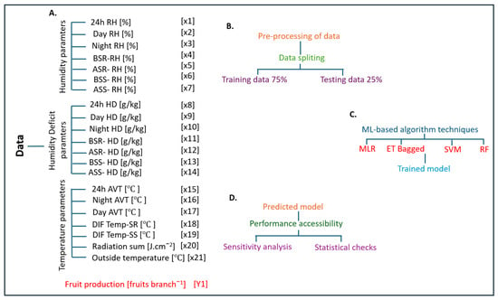
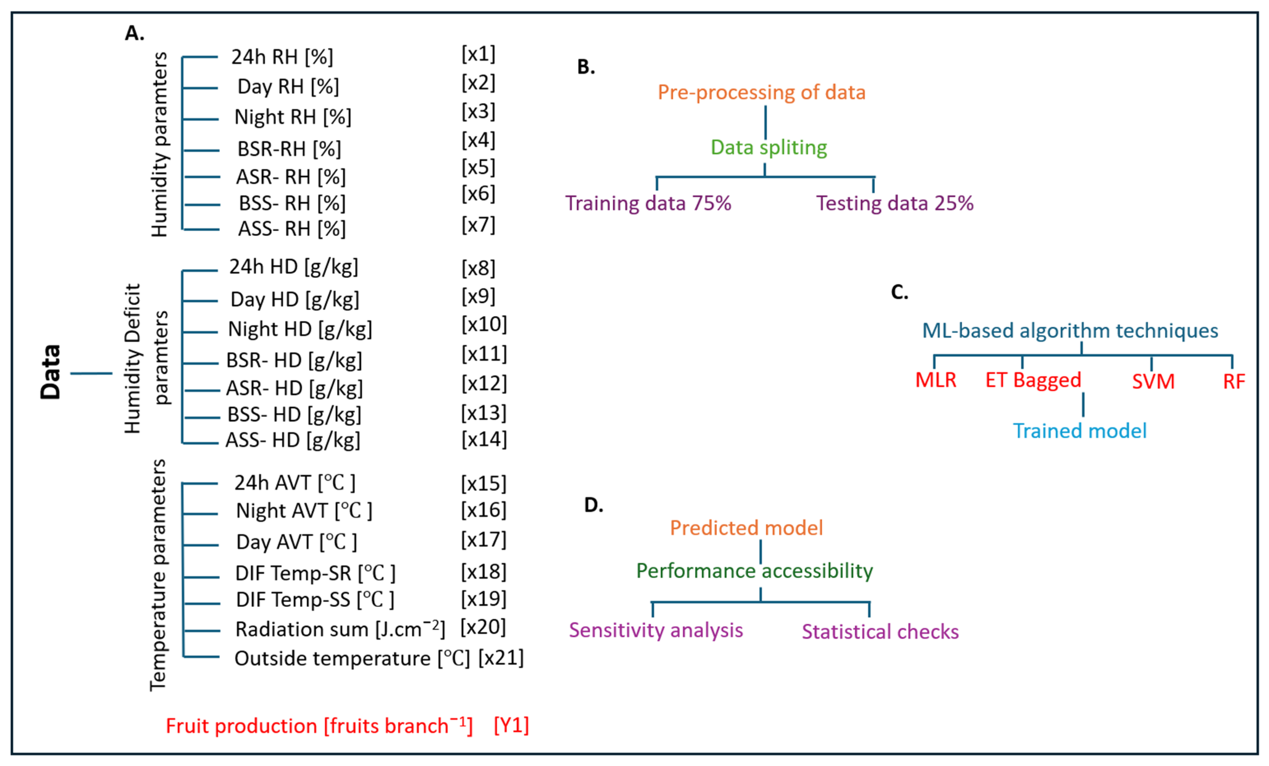
Twenty-one distinct factors were utilized in this research to evaluate paprika fruit production in Korea. The variables were divided into three groups: humidity factors in percentage [24 h RH, Day RH, Night RH, BSR-RH (before sunrise RH), ASR-RH (after sunrise RH), BSS-RH (before sunset RH), ASS-RH (after sunset RH)], humidity deficit factors in gram per kilogram [(24 HD, Day HD, Night HD, BSR-HD (before sunrise HD), ASR-HD (after sunrise HD), BSS-HD (before sunset HD), ASS-HD (after sunset HD)], and temperature variables in Celsius [(24 h AVT, Night AVT, Day AVT, DIF Temp-SR (sunrise), DIF Temp-SS (sunset), radiation sum, outside temperature)] (Figure 1A). The dependent variable was fruit production in numbers per square meter. All parameters were acquired on a weekly basis for four years.
Figure 1.
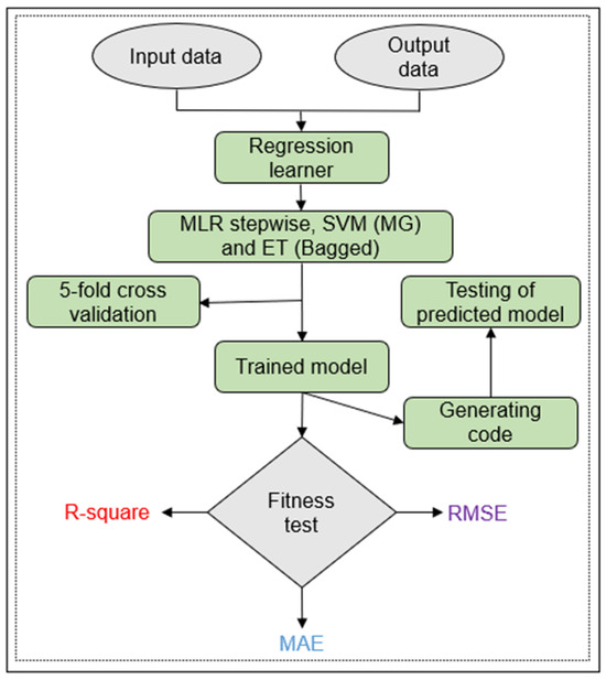
(A) Summary of the variables used in the prediction of paprika fruit production [Pn.f]. (B–D) Stepwise depictions of artificial intelligence approaches for development of prediction models.
Figure 1B–D depict the framework for creating a prediction model based on artificial intelligence utilizing several algorithms. Data collection is the first step in the process, after which it is pre-processed by selecting the affecting variables and removing randomness. The dataset is then split into two parts: 75% for training points and 25% for testing points. In order to generate a prediction model, the dataset is then dispersed and processed utilizing artificial intelligence-based computational techniques. Finally, a variety of statistical methods are employed to evaluate the model’s validity and ascertain its reliability. In this study, the total 4 year datasets of above-mentioned variables were used to develop AI-based models. Out of the 180 datasets, one hundred and thirty-five datasets from the first 3 years were used to train the model, while the remaining 47 datasets from the last year was used for testing purposes.
2.3. Data Range
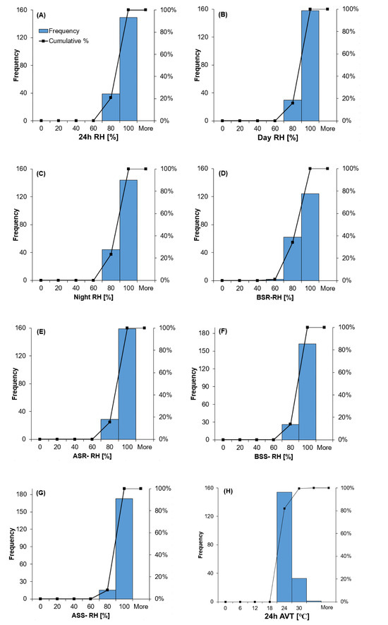
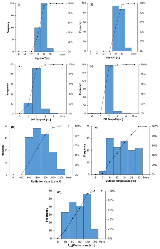
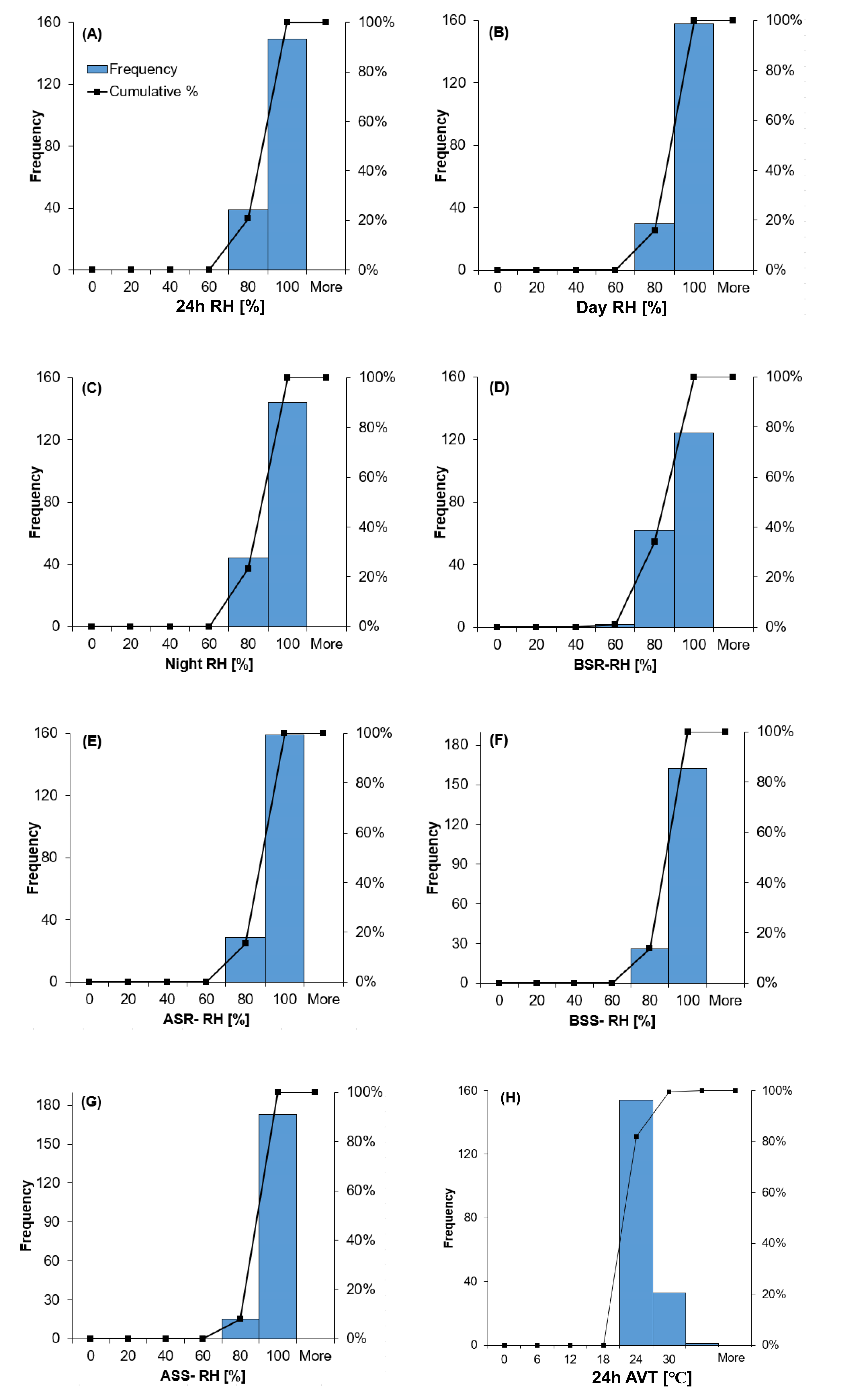
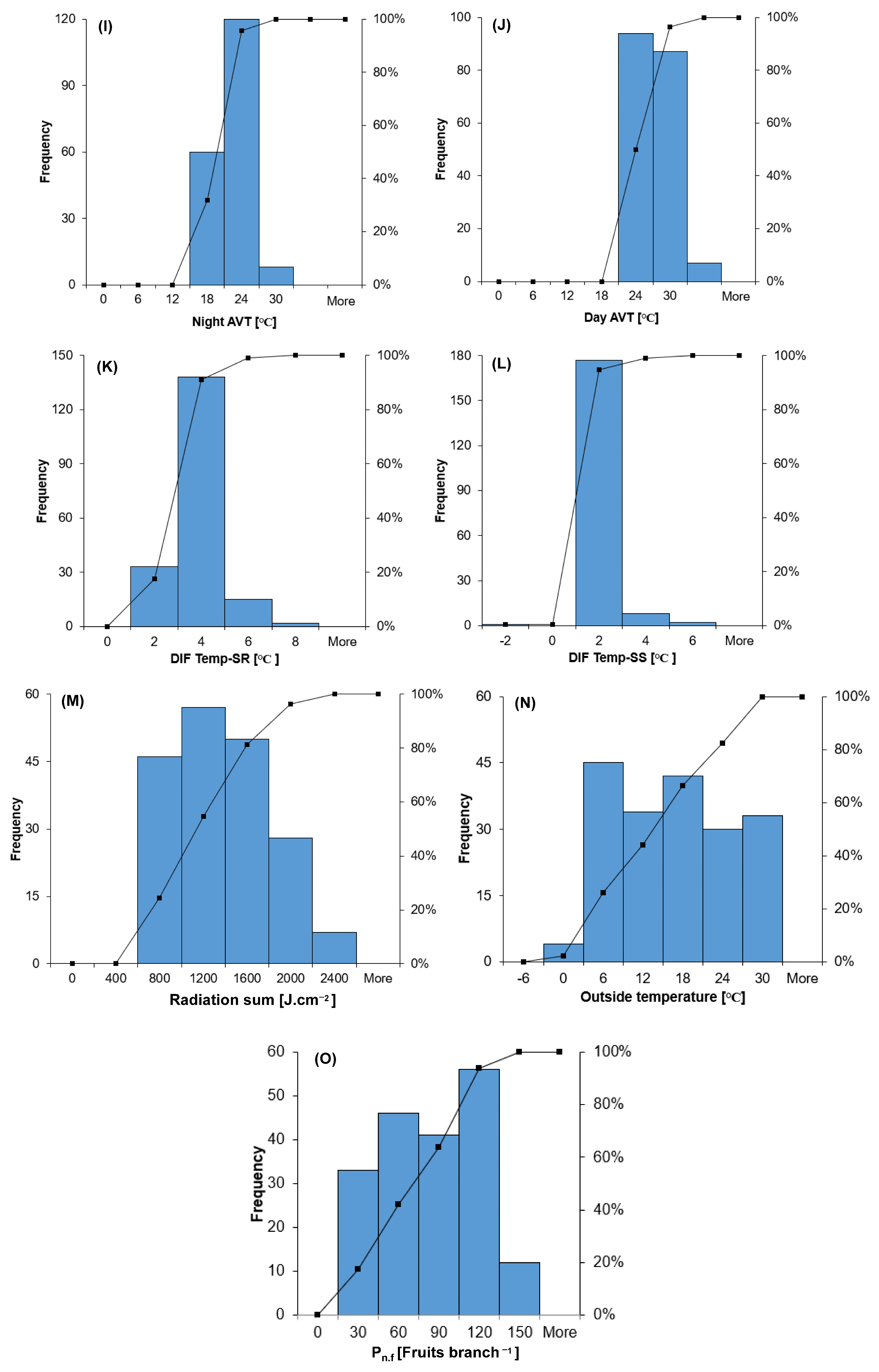
A histogram representing the frequency distribution for 4 years of data for each parameter is displayed in Figure 2 and Figure S1. The 24 h RH was determined to be 68.95–99.97%; the Day RH was noted between 66.45 and 100%; the Night RH ranged from 61.14 to 99.95%; the BSR RH ranged from 56.42 to 100%; the ASR RH ranged from 72.42 to 100%; the BSS RH was between 61.38 and 100% and the range of data points for ASS RH was between 70.15 and 95.37%. However, the data for relative humidity parameters, e.g., 24 h HD, Day HD, Night HD, BSR-HD, ASR-HD, BSS-HD, ASS-HD, were in the ranges of 0–7.19 g per kilogram, 0–10.40 g per kilogram, 0–4.99 g per kilogram, 0–5.94 g per kilogram, 0–4.70 g per kilogram, 0–11.26 g per kilogram, and 0–4.11 g per kilogram. Moreover, the temperature parameters, e.g., 24 h AVT, Night AVT, Day AVT, DIF Temp-SR, DIF Temp-SS, radiation sum, and outside temperature, ranged from 18.5 to 30.88 degrees centigrade, 16.37 to 27.51 degrees centigrade, 20.04 to 33.47 degrees centigrade, 0.74 to 6.17 degrees centigrade, −2.05 to 5.52 degrees centigrade, 417.64 to 23.06 joule per square centimeter, and −2.64 to 29.47 degrees centigrade. The paprika fruit production was recorded between 0.64 and 121.17 in numbers per square meter.
Figure 2.
Frequency histograms showing the observed distributions of 15 environmental predictors and one response variable (Pn.f). The predictors include relative humidity (RH; A–G), temperature-related variables (H–L), radiation sum (M), and outside temperature (N) while responsible variable consists of comulative fruit production (Pn.f) (O). Each histogram represents the frequency distribution of the collected observations within the measured range of the corresponding variables.
2.4. Pre-Processing of Data
Forecasting is the process of making predictions about the future, often using data from the past and present. Forecasting is not a new idea because data analysts frequently need to predict a variable from a group of predictors. Numerous studies have been conducted on crop growth predictions, many of which concentrate on Korea [27,28,31,32]. Numerous studies have demonstrated a robust correlation between climatic factors and paprika growth [31,32]. Nonetheless, the main objective of a successful forecast is to lower the forecasting error. Additionally, the errors obtained from projected models have been shown to be lower because machine learning techniques were used instead of econometric models.
Thus, based on weekly data collected over 4 years, the 21 predictors (relative humidity, humidity deficit, and temperature-related) were selected in this study to anticipate the cumulative fruit count (Pn.f). During weekly observation, the number of fruits harvested during the preceding week and the number of newly set fruits observed on the same branches were recorded and summed to obtain the weekly cumulative fruit count. A lead-time forecasting approach was adopted to predict subsequent paprika fruit production using weekly greenhouse environmental data. Environmental measurements recorded in a given week were matched with cumulative fruit-count observations obtained approximately 12 weeks later. This forecasting interval was determined based on observations from the present experiment, in which fruit set was first observed approximately 12 weeks after transplanting, falling in the range previously described for the 1st harvest as 11–14 weeks, depending on paprika variety [33]. Accordingly, the 12-week interval was used as an experimental basis for aligning environmental measurements with subsequent fruit production, rather than being considered a universally optimal forecasting horizon. The aligned dataset was subsequently used to develop and evaluate the regression models.
Table 2 and Table 3 display the basic statistical justifications of the environmental variables used in the prediction model’s training and testing stages, respectively. It is advised that the suggested stochastic relationships be used to assess and forecast the paprika output for the input data ranges indicated in Table 2 and Table 3.
Table 2.
Statistics of predictors (input parameters) and output data for training of Pn.f model.
Table 3.
Statistics of predictors (input parameters) and output data for testing of Pn.f model.
The Pearson correlation method is used to assess the level of reliance between the variables taken into consideration for modeling, according to [34]. R values, which range from −1 to +1, are used to assess the correlation strength. Positive and negative signs, respectively, show a trend toward growth or decline. A 0 in a Pearson correlation matrix denotes the absence of a relationship between the two variables. In contrast, a significant association is indicated by values close to 1. The following formula can be used to calculate the Pearson correlation coefficient mathematically:
where and are the mean values of the two variables, O and P, respectively. Based on the training dataset, the Pearson correlation matrix for Pn.f as the output factor/dependent variable and the environmental factors as the independent variables was obtained and is shown in Table S1.
2.5. Performance Evaluation
Equations (1)–(3) show that the model selection procedure in this work took into account statistical tests including RMSE, MAE, and R or R2 [35]. The best prediction models are said to have high R2 values that are near to 1 and low RMSE, MAPE, and MAE values [36].
MAE, or mean absolute error, is calculated as follows:
R2, or the coefficient of determination, is calculated as follows:
where
- = observed paprika fruit production for observation i,
- = predicted paprika fruit production for observation i,
- = mean of the observed fruit production values, and
- n = number of observations.
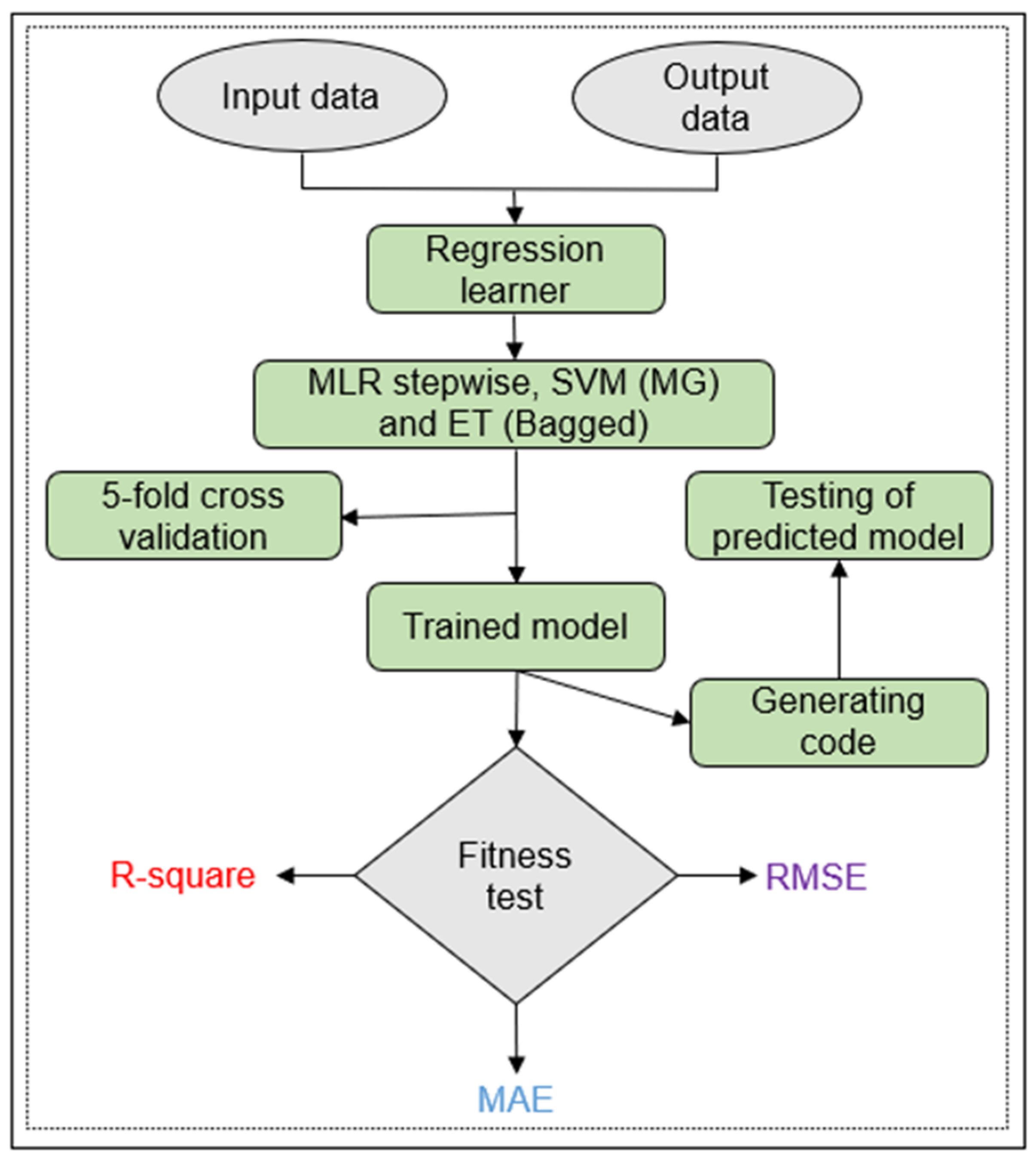
To evaluate model performance, the trained models developed in MATLAB Regression Learner were exported to the MATLAB workspace, and the generated code was used to predict paprika fruit numbers from the test dataset. These models were evaluated using MATLAB R2018, as shown in Figure 3. The RF model was implemented separately in Python 3.13, and its corresponding script is provided in the Supplementary file (Figure S2).
Figure 3.
Stepwise depiction of assessing the multiple linear regression (MLR), the linear support vector machine (SVM), and the ensemble tree bagging (ET Bagged) models.
2.6. Sensitivity Analysis (SA) and Parametric Study (PS) of Wp Prediction Model
To further evaluate the robustness and dependability of prediction models, parametric studies (PSs) and sensitivity analysis (SA) are employed. While parametric analysis shows how likely it is that the suggested prediction models will support or contradict physical occurrences, sensitivity analysis shows how significant independent variables are prioritized. Equation (4), which indicates that sensitivity values range from 0 to 1, was used in this study’s sensitivity analysis [36,37,38,39]. As stated in [39], values near 1 signify a strong sensitivity of the independent parameter, whereas values near zero imply that the parameter has minimal impact on the output parameter.
where characterizes the projected response attained from the Pn.f model and denotes the input parameters (environmental predictors). In addition, parametric analysis was used to determine whether the physical performance of the prediction model confirmed the physical process or simply showed a correlation [40,41,42].
2.7. Development of a Prediction Model
2.7.1. Multiple Linear Regression Model
For a parameter that depends on many input values, multiple linear regression analysis (MLR) is essentially utilized to provide a simple mathematical linear expression. The explanation of multiple linear regression analysis is found in Equation (5).
When , are the input variable, Y is the dependent parameter (output value), a is the constant found from the intercept, and , are the appropriate coefficients. The accuracy of the output value predicted by MLR is assessed by comparing it to the target value. Several statistical tests are used to assess the MLR model’s performance in order to confirm its ability to generalize. The procedure to analyze the MLR model with MATLAB version 2018 is depicted in Figure 3. A 3-year dataset was used to examine the MLR, and a 1-year testing dataset was used to assess it. The training model from Regression Learner was first exported to the MATLAB workspace in order to test the predicted model. The process was then finished by comparing the testing input dataset with the trained model, which was created using automatically generated code.
2.7.2. Support Vector Regression
Support vector regression (SVR) was used to forecast constant paprika fruit production from greenhouse environmental factors. A Gaussian kernel was used to model potentially nonlinear associations between the input factors and the response variable. The SVR model evaluates a regression function by maintaining model flatness against deviations exceeding the specified epsilon-insensitive loss threshold. The Medium Gaussian SVM model was selected in MATLAB Regression Learner, with a reported kernel scale of 4.8, automatic box constraint and epsilon settings, and predictor standardization enabled (Figure 3).
The general regression function is represented by Equation (6).
- where x represents environmental measurements,
- (x) represents their transformed features,
- calculates a weighted combination of those features, and
- b adjusts the final prediction by adding a constant.
MATLAB processed the data and created a predicted model based on Figure 3.
2.7.3. Tree Ensemble Methods: Bagging
One of the main problems with the decision tree model is the substantial degree of outcome variance. If the data is divided into training and testing datasets, fitting a decision tree to different datasets may produce different results each time. Several ensemble strategies are used to reduce disparities in the data, but only the bagging strategy is used in this work.
Bagging is the practice of employing the bootstrap method to repeatedly generate B sets of unique bootstrapped training data from a single training dataset. After building a unique decision tree from the B training datasets, the next step in the bagging process is to average the sets of observations to reduce variances and increase prediction accuracy. Using a bootstrapping dataset, each tree in bagging is built separately from the others. In contrast, the boosting strategy grows the trees one after the other. The trees produced with the boosting strategy are largely dependent on earlier trees. The output of the ensemble model is expressed in the following Equation (7):
where b is the number of repetitive times from 1 to B and λ is the shrinkage parameter, with a typical value set at between 0.01 and 0.001.
f∧(x) = ∑b = 1Bλfb∧(x)
2.7.4. Random Forest
Random Forest regression (RF) is an ensemble learning method that assembles the predictions of multiple decision trees to evaluate a continuous response variable. In this study, RF was used to predict paprika fruit production Pn.f from greenhouse environmental variables. Each regression tree was trained using a bootstrap sample of the training dataset, while an arbitrarily selected subset of predictor variables was measured at each split. This process introduces disparity among the trees and helps decrease the dependency on any single tree. The final prediction is obtained by averaging the numerical predictions produced by all trees in the forest.
The Random Forest regression prediction is obtained by averaging the predictions of all regression trees, as expressed in Equation (8).
where
- ŷ(x) = predicted paprika fruit production,
- x = vector of greenhouse environmental input variables,
- B = total number of regression trees, b = index of an individual tree, from 1 to B, and
- fb (x) = prediction generated by the b-th regression tree.
3. Results and Discussion
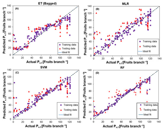
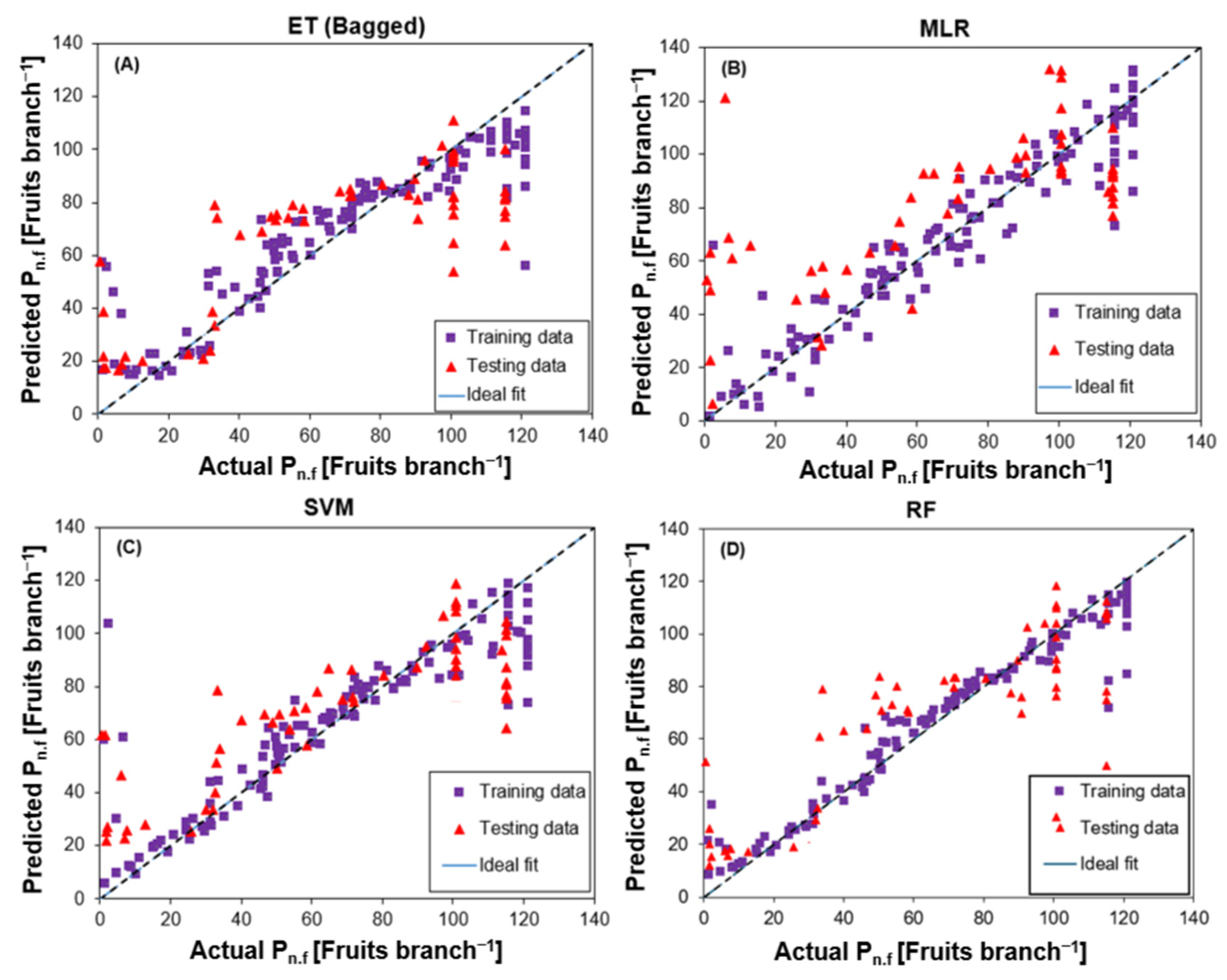
Based on the environmental indicators mentioned above, the results of the ET (Bagged), MLR, SVM, and RF models for the prediction of Pn.f production versus the training and testing datasets are shown in Figure 4. Nearly 1:1 (perfect fit) predicted responses are seen in all the models with improved generalizability. Table 4 lists the optimal tuning parameter values for RF, SVM, and ET (Bagged). The ET (Bagged) and SVM models were trained in MATLAB using Regression Learner, and due to Regression Learner’s built-in function, the parameters were automatically adjusted. However, when Regression Learner is trained, the other hyperparameters are automatically turned off. The 5-fold cross-validation was used to address the complicated training dataset and reduce the prediction efficiency error. This approach optimizes model complexity to minimize estimation or classification errors on unobserved data, according to [43]. By recognizing the trade-off between bias and variance, this strategy can also be used to avoid overfitting and selection bias [44]. However, using the GridSearchCV algorithm for the RF model, the parameters were adjusted in Python. To assess each model’s performance, Table 5 presents a summary of the statistical check values. When comparing the RF model to other prediction models, the SVM model scores lowest in terms of higher rank, while the RF model yields the best results when using the training data. In contrast to the other estimated models, SVM and RF performed the best in terms of R2 and lowest error while testing the trained model, with MLR placing fourth. Refs. [45,46] state that all the statistical check values support the current study’s prediction models’ acceptance criteria (RMSE and MAE values should be sufficiently low, and the R2 value is closer to 1).
Figure 4.
Performance evaluation of prediction models based on training and testing data: (A) ET (Bagged) model; (B) MLR model; (C) SVM model; and (D) RF model.
Table 4.
Best parameters used for selection of ET (Bagged), RF and SVM models.
Table 5.
Performance comparison of the models.
However, SVM achieved the highest testing (R2) value (0.677), while RF exhibited the lowest RMSE (22.08) and MAE (16.89). These findings demonstrate that the model performance differed across the evaluation metrics, with SVM performing best in terms of testing (R2), while RF performed best in terms of testing RMSE and MAE. However, R2 values represent the coefficient of determination and should not be interpreted directly as percentages of prediction accuracy. The RF model showed a decrease in R2 from 0.950 during training to 0.668 during testing, indicating reduced predictive efficiency on the unseen season and likely overfitting. Other limitations are interseasonal disparity in greenhouse environmental conditions and fruit production, or a combination of both factors. The partial sample size relative to the 21 forecasters may also have affected the model generalizability. Although RF outperformed MLR across all the testing metrics, further research using additional growing seasons and reduced-variable models is needed to assess the robustness of these predictions and govern whether the model complexity can be reduced without losing performance.
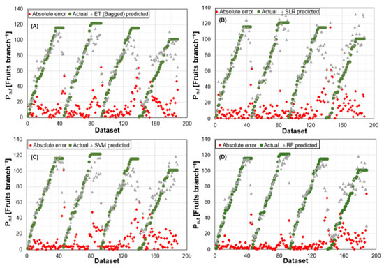
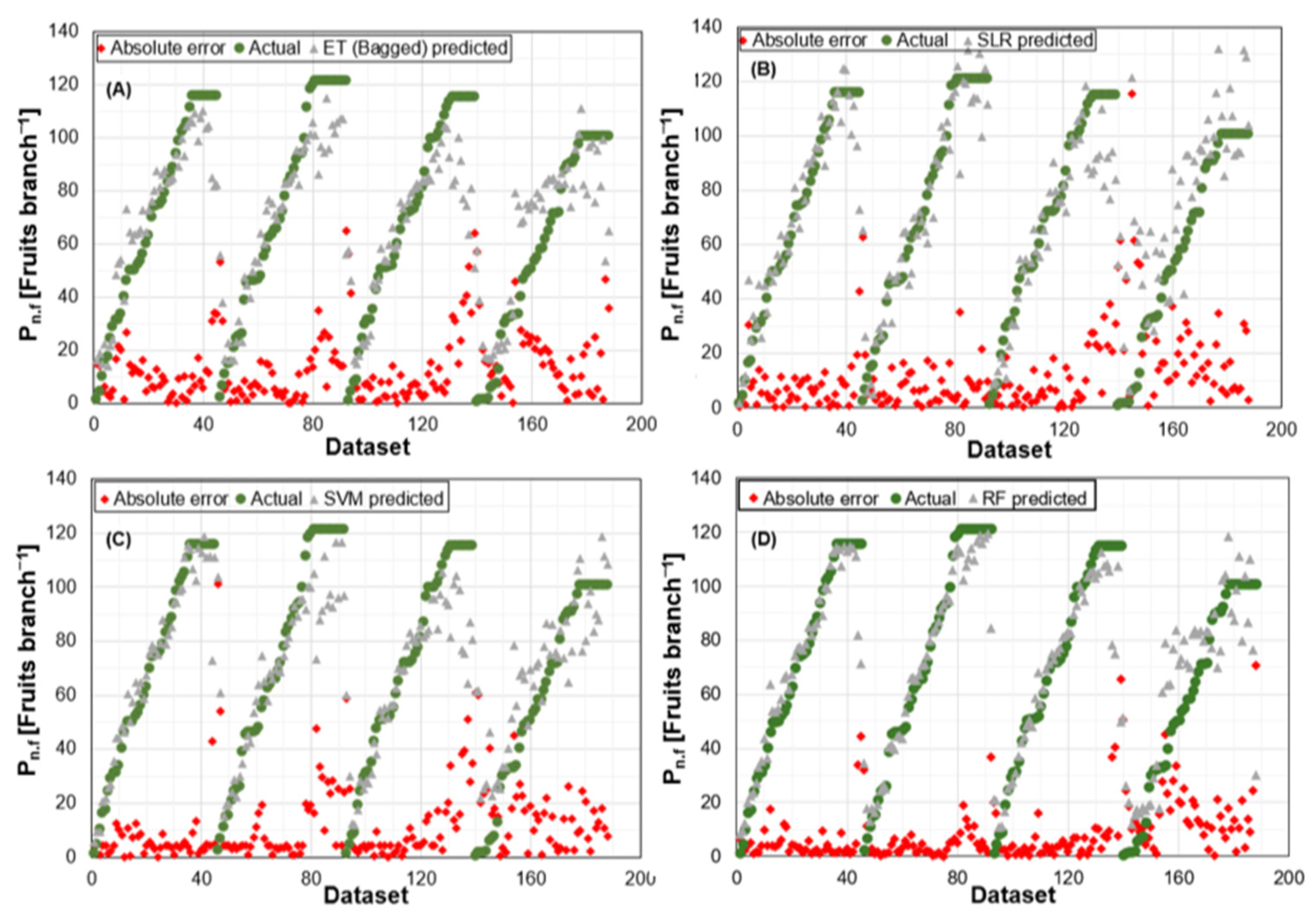
The ET (Bagged) model has an R2 of 0.843 for the trained model and also passes statistical tests. The SVM and RF models work well with a fraction of the training data, even though their R2 was higher than those of other predicted models [43]. However, ET (Bagged) is a tree-based ensemble model that uses sampling with replacement to create several trees from the training data in an effort to lower prediction variance and hence improve the model’s generalizability [47]. RF, on the other hand, is a particular kind of bagging ensemble in which the number of predictors selected as split candidates in each iteration is determined by a random value for each tree [48]. This makes RF superior to bagging since Random Forest de-correlates the trees. Moreover, RF computes error rates using observations (out-of-bag observations) that are not part of the bootstrapped samples [49,50]. Similarly, it is claimed that SVM outperforms multiple linear regression in terms of consistency and performance. Furthermore, the model performance differences between Random Forest and SVM are not substantial [51]. Unlike conventional linear regression models, Random Forest decision trees and support vectors are capable of handling non-linear connections. In addition, when overfitting is avoided, non-parametric Random Forest and SVM outperform linear regression. In comparison to Random Forest and SVM, MLR scored worse on the validation set, suggesting that the calibration model exhibited some overfitting and was not as effective as Random Forest [52]. The kind of dataset, such as discrete or continuous, affects these models’ accuracy and performance [53]. In summary, a previous study [43] found that the SVM and RF algorithms are most appropriate for creating the best model, given the size and particular type of dataset utilized in this study. Despite the small size of the dataset, the acquisition of crucial input parameters may improve the effectiveness of the SVM and RF models in the current study. Figure 5A–D compare the observed and predicted paprika Pn.f for the four models. The mean absolute errors were 13.61, 12.65, 11.85, and 8.86 fruits m−2 for ET (Bagged), MLR, SVM, and RF, respectively. RF showed the lowest prediction error, followed by SVM, MLR, and ET (Bagged).
Figure 5.
Plots of absolute errors for the prediction models against actual and forecasted data: (A) ET (Bagged); (B) MLR; (C) SVM; and (D) RF.
Figure S3 shows all four models’ simulated and real responses to the training and testing datasets. The fact that the actual and predicted reactions overlapped shows a strong connection and coherence between the two. In this case, MLR and ET (Bagged) are typically less accurate, and their test findings differ greatly from the actual dataset. However, the responses from the SVM and RF models confirm their superiority and are close enough.
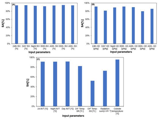
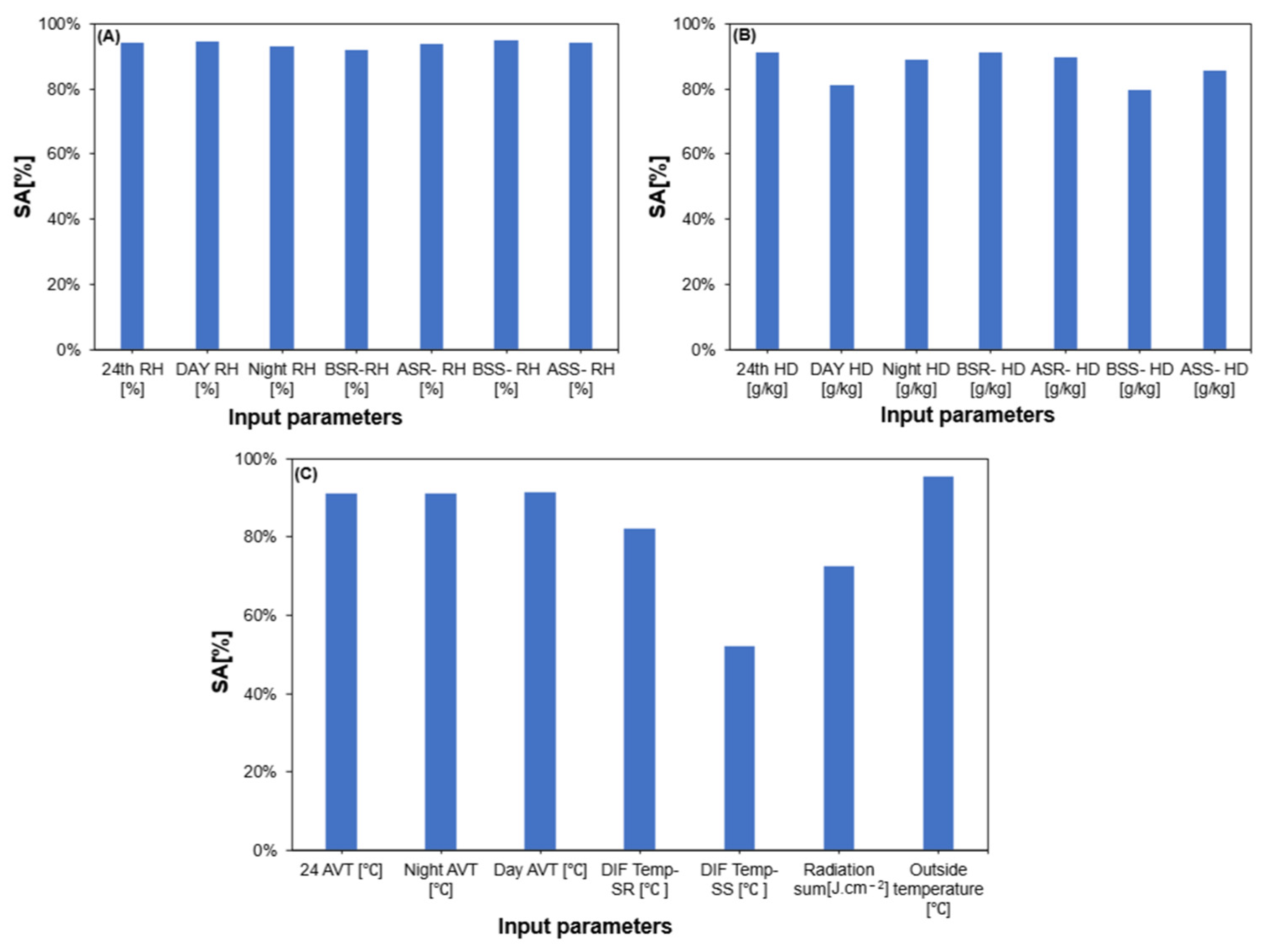
Figure 6 shows the results of a sensitivity analysis conducted on the SVM model. To keep this study as short as possible, the sensitivity analysis against ET (Bagged), RF, and MLR was excluded. Although the sensitivity analysis indicated relatively high values for several environmental predictors, these results should be interpreted with caution because of the strong interdependence among the input variables. As presented in Table S1, Night RH and BSR-RH showed a strong positive correlation (r = 0.961), while 24 h average temperature and daytime average temperature were also strongly correlated (r = 0.970). Similarly, Day RH and Day HD exhibited a strong negative correlation (r = −0.872). These relationships suggest that the environmental predictors contain overlapping information. Consequently, the reported sensitivity rankings reflect numerical associations between the individual predictors and the model-predicted response, rather than their independent contributions to paprika fruit production. The rankings therefore provide descriptive information about the modeled relationships but should not be interpreted as evidence of separate causal effects.
Figure 6.
Role of input parameters in SVM-based Pn.f model: (A) relative humidity related parameters; (B) humidity deficit related parameters; (C) Temperature related parameters.
The sensitivity analysis was used to quantify the numerical association between each environmental predictor and the model-predicted paprika fruit production. The terms in Equation (4) represent the observed environmental input values and the corresponding model-predicted responses across the available observations. The resulting sensitivity values were used for descriptive comparison among the environmental predictors rather than for quantifying their independent contributions to the predicted response.
It is important to note that several environmental variables, particularly relative humidity, humidity deficit, and temperature, are strongly interrelated. Therefore, the sensitivity values may reflect overlapping information among the predictors and should not be interpreted as evidence of independent causal effects. The Pearson correlation matrix (Table S1) was considered when interpreting these relationships.
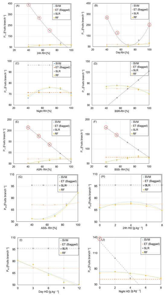
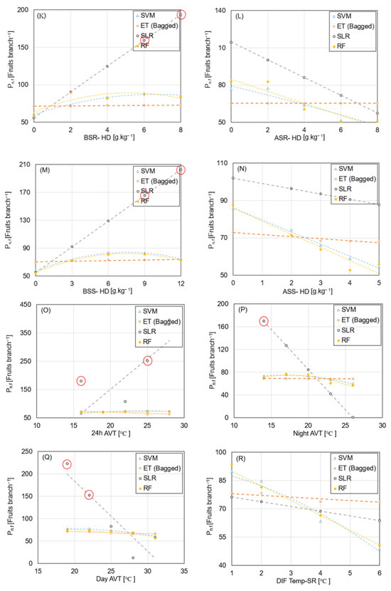
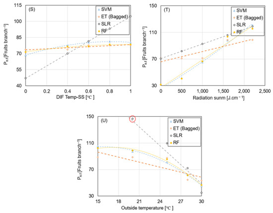
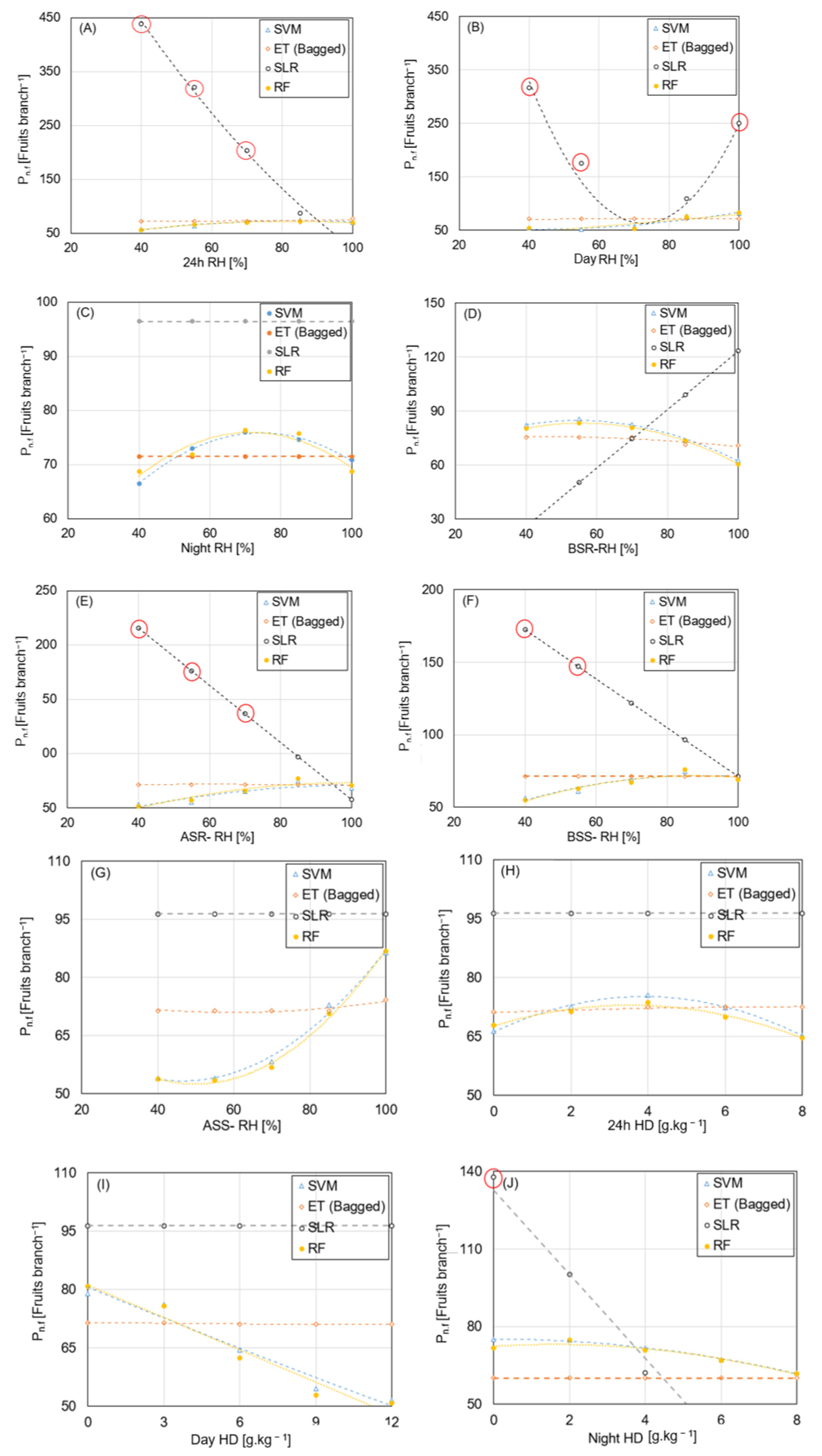
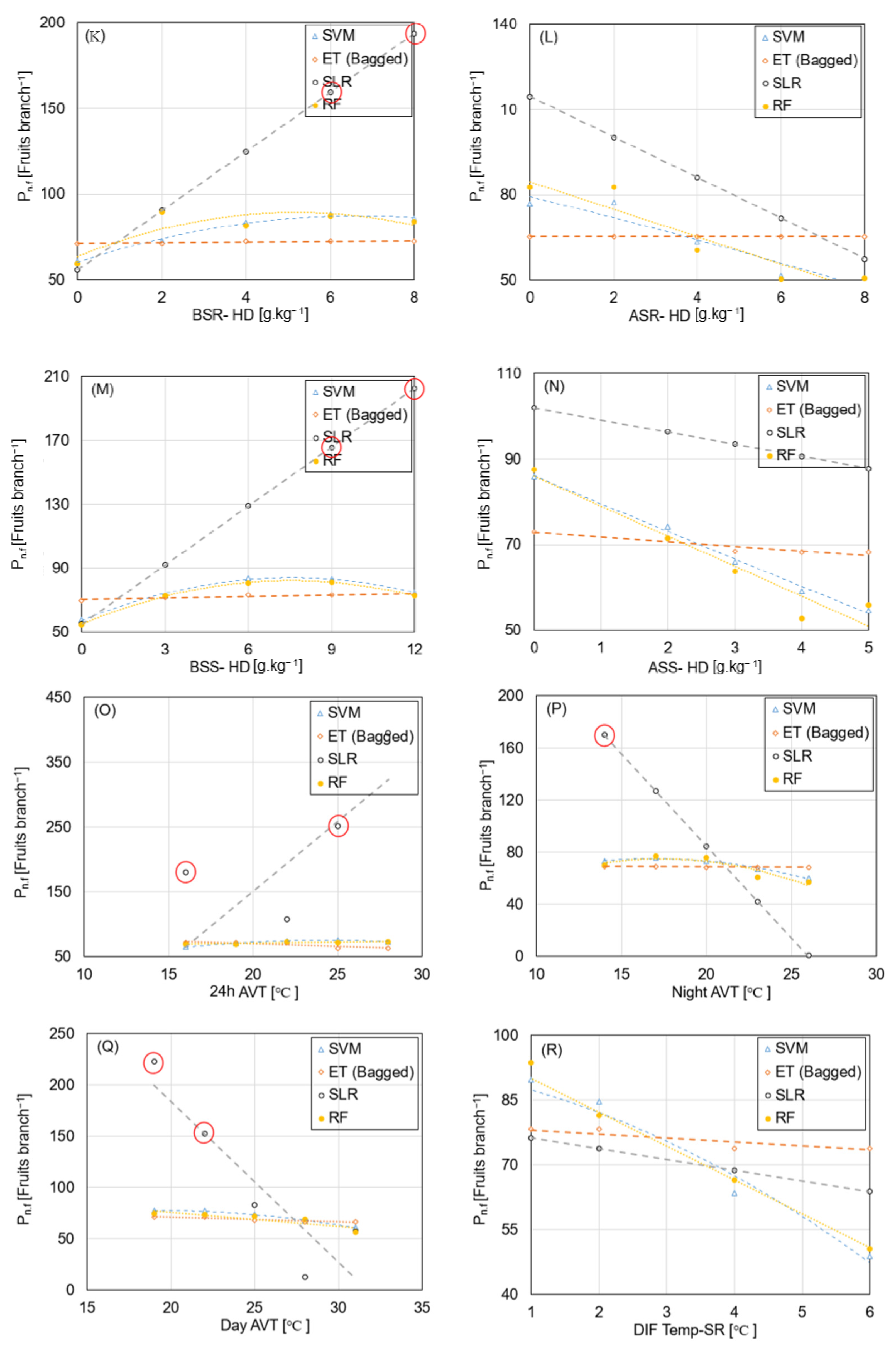
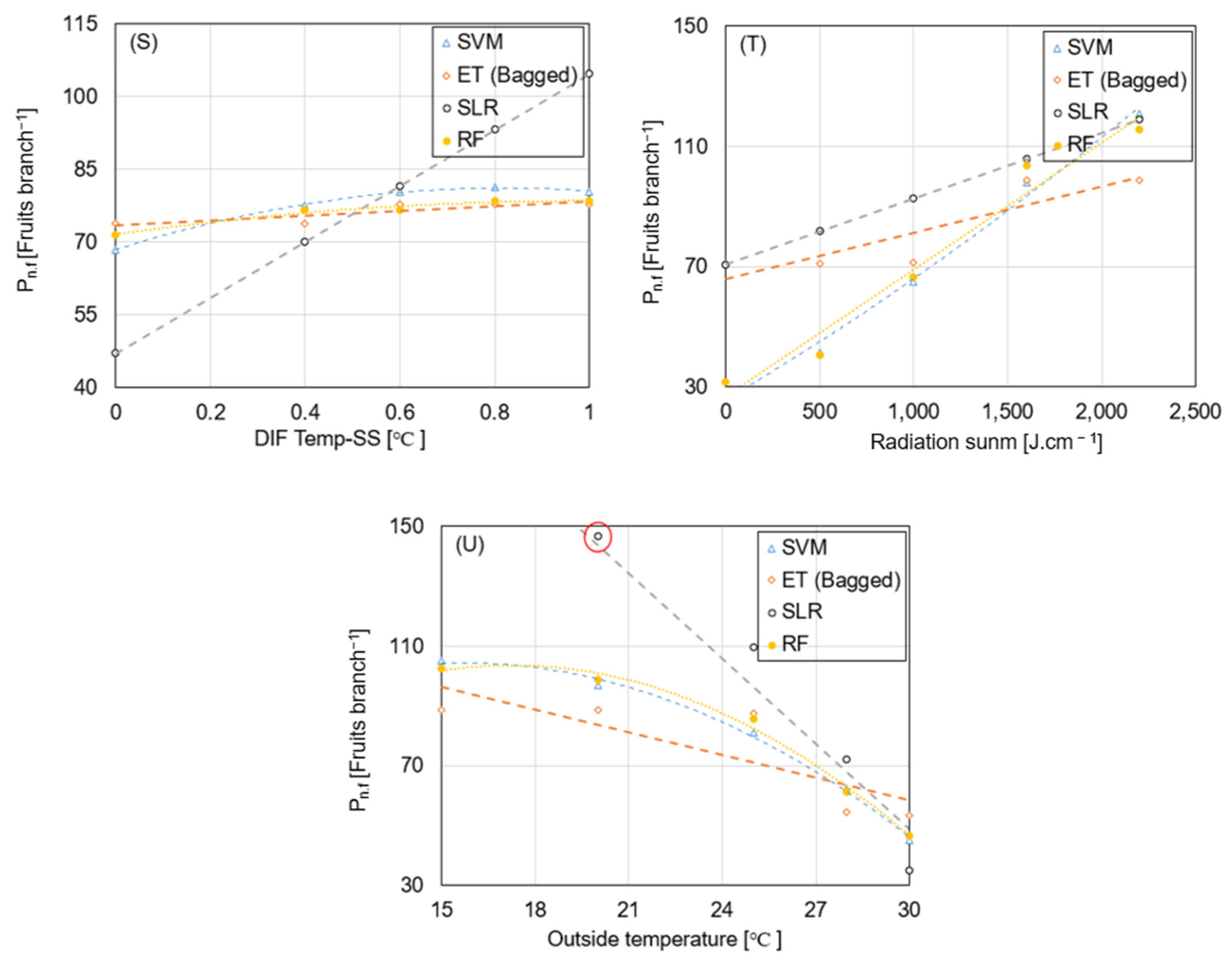
Figure 7A–U presents the results of the parametric analysis performed using the ET (Bagged), MLR, SVM, and RF models. In this analysis, one environmental predictor was varied while the remaining predictors were held at their respective mean values, and the resulting changes in the predicted paprika fruit production [Pn.f] were examined. The plots therefore illustrate how the model predictions respond to changes in individual predictors under the specified conditions. However, because greenhouse environmental variables are interrelated, particularly relative humidity (RH), humidity deficit (HD), and temperature, the combinations created by varying one variable independently may not always represent conditions that occur in a real greenhouse. Furthermore, the curves indicate model-derived responses rather than empirically measured responses under controlled environmental conditions. Accordingly, the apparent peaks and turning points should be interpreted as predicted response patterns, not as experimentally produced optimum conditions.
Figure 7.
One-at-a-time (OAT) parametric sensitivity analysis of predicted paprika fruit production (Pn.f) using Random Forest (RF), support vector machine (SVM), ensemble trees (ETs; Bagged), and multiple linear regression (MLR) models. Each panel (A–U) represents one of the 21 environmental predictors: relative humidity (RH; A–G), humidity deficit (HD; H–N), temperature-related variables (O–S), radiation sum (T), and outside temperature (U). Red circles indicate predictions outside the observed cumulative fruit-count range, Pn.f. This occurred due to the lower accuracy in the prediction of Pn.f by SLR. SLR did not outperform RF, SVM, and ET (Bagged).
The RH-related sensitivity plots (Figure 7A–G) indicate that predicted paprika fruit production generally increased over portions of the evaluated RH ranges, with a change in the predicted response occurring around the 60–80% RH range. This pattern suggests that the RH-related variables were influential in the model predictions under the conditions examined. However, the indicated range should not be interpreted as a universal optimum for paprika production, particularly because the analysis varied each RH-related predictor independently of the other environmental variables. Relative humidity can influence transpiration, plant water relations, and reproductive processes, but its effects depend on temperature and other greenhouse conditions. Previous studies have reported relationships between greenhouse humidity, plant growth, sap flow, and crop performance [54,55,56,57]. Nevertheless, excessively high humidity can interfere with pollen release and reproductive development and may favor disease development when condensation occurs [58,59,60]. Thus, the model-derived patterns should be considered alongside the actual RH values and fruit counts observed in this study as well as the physiological context reported in the literature. Predictions outside the observed environmental or fruit-count ranges should be treated cautiously because they are not directly supported by the experimental observations.
The HD-related plots (Figure 7H–N) also show variation in the predicted fruit production across the evaluated HD values, with a potentially favorable response pattern appearing within approximately 2–7 g kg−1 in the model-based analysis. This range should be regarded as an exploratory model-derived indication rather than a confirmed optimum. HD is related to atmospheric evaporative demand and is influenced by temperature and RH; therefore, its relationship with crop performance cannot be interpreted independently of these variables. Related research on greenhouse crops has shown that vapor pressure deficit (VPD) can affect transpiration, water transport, mineral distribution, and fruit development, and that both very low and very high VPD conditions may be unfavorable [61,62,63,64,65,66]. However, VPD and HD are not identical measures, and the values reported for VPD cannot be directly treated as equivalent to the HD values used in the present study. The physiological implications of the predicted HD response should therefore be interpreted with reference to the environmental conditions actually observed in the greenhouse. Further experiments are required to determine whether the model-suggested range consistently supports improved paprika fruit production.
The temperature-related plots indicate that the predicted fruit production varied with 24 h average temperature, night temperature, and daytime temperature (Figure 7O–Q). The model predictions suggested comparatively favorable responses within the evaluated ranges of approximately 15–25 °C for 24 h average temperature, 15–20 °C for night temperature, and 20–25 °C for daytime temperature. These ranges describe patterns observed in the model-generated curves and should not be considered experimentally established temperature optima. Previous research has reported associations between paprika production and temperature, including reduced production under excessively high daytime and nighttime temperatures [6,32,67]. High air and root-zone temperatures may also impair root activity and plant growth [68,69,70,71]. These findings provide the physiological context for interpreting the model predictions, but they do not independently validate the precise temperature ranges identified by the OAT analysis. In addition, the DIF-related plots (Figure 7R,S) suggest changes in predicted fruit production across the evaluated temperature-difference variables. These responses indicate model sensitivity to the selected DIF predictors; however, they do not establish that lower DIF values directly increase fruit number. The interpretation of these patterns requires consideration of the observed DIF ranges and the relationships among temperature, crop development, and other environmental variables.
The radiation-related plot (Figure 7T) indicates that the predicted paprika fruit production increased over part of the evaluated radiation-sum range before the response changed. This pattern is consistent with the established role of solar radiation in photosynthesis and crop biomass accumulation. Previous studies have associated insufficient solar radiation with reduced crop productivity, including paprika production [6,72]. Nevertheless, the apparent turning point in the model-created curve should not be interpreted as a confirmed radiation optimum. Its importance depends on whether the matching radiation values and predicted fruit counts fall within the ranges denoted by the observed data. Similarly, the outside-temperature response (Figure 7U) should be interpreted as a model-derived relationship rather than evidence of an independent causal effect, because outside temperature may be associated with other greenhouse environmental conditions.
Limitations and Future Prospects
The following problems should be resolved in the future to increase the accuracy and certainty of the expected model. First, a wider selection of variables, such as planting season, breeding lines (varieties), plant height, fruit weight and fruit set, etc., are needed to improve the model’s robustness. Correct and sufficient data for these predictors is also crucial for the projected model to have higher accuracy and certainty.
Second, the ET (Bagged) model performed inefficiently due to the current study’s smaller and random dataset. Both the accuracy of the model and the disparity between the sensitivity and parametric analysis results can be reconciled with the use of big, high-quality datasets. Similarly, higher-quality datasets and invariance in their data ranges can further enhance the accuracy of RF and SVM.
Third, despite preserving the chronological order of the data and evaluating the model performance on an independent growing season, the regression models did not explicitly capture the full temporal dynamics of paprika fruit development. Cumulative fruit production may be affected by environmental conditions over the preceding several weeks, which may not be fully represented by a fixed 12-week forecasting horizon. Future research should therefore investigate different forecasting horizons and incorporate environmental measurements from multiple preceding weeks to determine whether accounting for these temporal relationships can improve prediction performance. However, the time-lagged approach usually requires a large sample size (almost 15–20 year datasets) for better forecasting.
4. Conclusions and Recommendations
This study compared the predictive performance of multiple linear regression (MLR), support vector machine (SVM), ensemble tree bagging (ET Bagged), and Random Forest (RF) models for estimating paprika fruit production (Pn.f) from greenhouse environmental data. On the independent test dataset, SVM achieved the highest coefficient of determination (R2 = 0.677), while RF produced the lowest root mean square error (RMSE = 22.08) and mean absolute error (MAE = 16.89). These findings suggest that SVM and RF provided comparatively favorable predictive performance under the conditions evaluated. However, the difference between the training and testing performance, particularly for RF, highlights the need for validation using additional growing seasons to determine the models’ generalizability.
The sensitivity analysis highlighted several relative humidity (RH), humidity deficit (HD), and temperature-related predictors, including Day RH, BSS-RH, 24 h RH, ASS-RH, ASR-RH, Night RH, BSR-RH, 24 h HD, Night HD, BSR-HD, BSS-HD, 24 h AVT, Night AVT, Day AVT, DIF Temp-SS, radiation sum, and outside temperature. These variables showed notable influences on the model predictions under the sensitivity-analysis procedure. However, the rankings represent model sensitivity to changes in the selected inputs rather than independent causal effects on paprika fruit production. Since RH, HD, and temperature are interrelated, the results should be interpreted cautiously, particularly where changes in one predictor while holding others constant may represent environmental conditions that are uncommon in an actual greenhouse. Accordingly, the predicted response patterns and turning points should be considered exploratory indications rather than experimentally established optimum conditions. Further validation under controlled greenhouse conditions is required to determine whether the suggested environmental ranges improve fruit production.
Supplementary Materials
The following supporting information can be downloaded at: https://www.mdpi.com/article/10.3390/agriculture16212407/s1.
Author Contributions
I.Y.: Conceptualization, investigation, methodology, writing—original draft. G.K.: Investigation, methodology, writing—review and editing. B.L.: Conceptualization, data curation, project administration, supervision. All authors have read and agreed to the published version of the manuscript.
Funding
This work was supported by the Institute of Information & Communications Technology Planning & Evaluation (IITP)-Innovative Human Resource Development for Local Intellectualization program grant funded by the Korean government (MSIT) (IITP-2025-RS-2020-II201489).
Institutional Review Board Statement
Not applicable.
Data Availability Statement
Descriptive metrics of the dataset are provided in the article and the Supplementary Materials.
Conflicts of Interest
Author Gyuha Kim was employed by the company Artfarm Agricultural Company. The remaining authors declare that the research was conducted in the absence of any commercial or financial relationships that could be construed as a potential conflict of interest.
Abbreviations
| Pn.f | Paprika cumulative fruit count |
| MLR | Multiple linear regression |
| SVM | Support vector machine |
| ET Bagged | Ensemble tree bagging |
| RF | Random Forest |
| 24 h RH | 24 h relative humidity |
| Day RH | Day time relative humidity |
| Night RH | Nighttime relative humidity |
| BSR-RH | Relative humidity before sunrise |
| ASR-RH | Relative humidity after sunrise |
| BSS-RH | Relative humidity before sunset |
| ASS-RH | Relative humidity after sunset |
| 24 h HD | 24 h humidity deficit |
| Day HD | Day time humidity deficit |
| Night HD | Nighttime humidity deficit |
| BSR-HD | Humidity deficit before sunrise |
| ASR-HD | Humidity deficit after sunrise |
| BSS-HD | Humidity deficit before sunset |
| ASS-HD | Humidity deficit after sunset |
| 24 h AVT | 24 h average temperature |
| Night AVT | Night average temperature |
| Day AVT | Day time average temperature |
| DIF Temp-SR | Difference in temperature relative to sunrise |
| DIF Temp-SS | Difference in temperature relative to sunset |
| SA | Sensitivity analysis |
| PA | Parametric analysis |
References
- Hayat, U.; Ali, S.; Mateen, A.; Bilal, H. The Role of Agriculture in Poverty Alleviation: Empirical Evidence from Pakistan. Sarhad J. Agric. 2019, 35, 1309–13015. [Google Scholar] [CrossRef] [Scilit]
- Valdes, A. Food Security for Developing Countries; Routledge: Abingdon-on-Thames, UK, 2019. [Google Scholar]
- Ghavate, S.; Joshi, H. Smart Farming Using IoT and Machine Learning with Image Processing. Int. J. Curr. Eng. Technol. 2021, 8, 15–19. [Google Scholar] [CrossRef] [Scilit]
- Yu, J.; Wu, J. The Sustainability of Agricultural Development in China: The Agriculture–Environment Nexus. Sustainability 2018, 10, 1776. [Google Scholar] [CrossRef] [Scilit]
- KATI. Paprika. 2023. Available online: https://www.kati.net/product/basisInfo.do?lcdCode=MD147 (accessed on 8 June 2023).
- Kim, M.; Lee, Y.B.; Choi, K.Y. Effects of Greenhouse Temperatures and Solar Irradiance Levels on the Monthly Production of Summer-Cultivated Paprika. Hortic. Sci. Technol. 2024, 42, 339–349. [Google Scholar] [CrossRef] [Scilit]
- Bakker, J.C.; van Uffelen, J.A.M. The Effects of Diurnal Temperature Regimes on Growth and Yield of Glasshouse Sweet Pepper. Neth. J. Agric. Sci. 1988, 36, 201–208. [Google Scholar] [CrossRef] [Scilit]
- Rural Development Administration (RDA). Sweet Pepper. Agricultural Technology Guide 124; RDA: Jeonju-si, Republic of Korea, 2020.
- Bakker, J.C. The Effects of Temperature on Flowering, Fruit Set and Fruit Development of Glasshouse Sweet Pepper (Capsicum annuum L.). J. Hortic. Sci. 1989, 64, 313–320. [Google Scholar] [CrossRef] [Scilit]
- Dat, J.; Vandenabeele, S.; Vranová, E.; Van Montagu, M.; Inzé, D.; Van Breusegem, F. Dual Action of the Active Oxygen Species during Plant Stress Responses. Cell. Mol. Life Sci. 2000, 57, 779–795. [Google Scholar] [CrossRef] [Scilit] [PubMed]
- Lim, C.S. Effect of Low Night Temperature on Reproductive Organ Development in Relation to Pollen Viability of Bell Pepper. J. Life Sci. 2009, 19, 581–586. [Google Scholar] [CrossRef] [Scilit]
- Korea Meteorological Administration (KMA). Open MET Data Portal. 2023. Available online: https://data.kma.go.kr/climate/RankState/selectRankStatisticsDivisionList.do?pgmNo=179 (accessed on 22 July 2023).
- Adams, S.R.; Cockshull, K.E.; Cave, C.R.J. Effect of Temperature on the Growth and Development of Tomato Fruits. Ann. Bot. 2001, 88, 869–877. [Google Scholar] [CrossRef] [Scilit]
- Lee, J.W.; Kim, H.C.; Jeong, P.H.; Ku, Y.G.; Bae, J.H. Effects of Supplemental Lighting of High-Pressure Sodium and Lighting Emitting Plasma on Growth and Productivity of Paprika during the Low-Radiation Period of Winter Season. Korean J. Hortic. Sci. Technol. 2014, 32, 346–352. [Google Scholar] [CrossRef] [Scilit]
- Kim, E.J.; Lee, B.S.; Jeon, Y.H.; Ju, S.H.; Go, Y.; Park, J.S.; Lee, J.W.; Yang, H.J.; Na, H.Y. Comparison of Photosynthetic Efficiency and Growth Characteristics of Paprika in Semi-Closed versus Conventional Greenhouses. Hortic. Environ. Biotechnol. 2023, 64, 977–985. [Google Scholar] [CrossRef] [Scilit]
- Kim, Y.H.; Yang, H.C.; Yang, S.H.; Kim, D.H.; Jang, D.C. Comparison of Growth and Fruiting Characteristics between Cultivars for the Selection of Appropriate Domestic Cultivars when Cultivating Paprika in High-Temperature Periods. Korean J. Hortic. Sci. Technol. 2023, 41, 674–685. [Google Scholar] [CrossRef] [Scilit]
- Liu, H.; Xiong, W.; Mottaleb, K.A.; Krupnik, T.J.; Burgueño, J.; Pequeno, D.N.; Wu, W. Contrasting Contributions of Five Factors to Wheat Yield Growth in China by Process-Based and Statistical Models. Eur. J. Agron. 2021, 130, 126370. [Google Scholar] [CrossRef] [Scilit]
- Wallach, D.; Martre, P.; Liu, B.; Asseng, S.; Ewert, F.; Thorburn, P.J.; van Ittersum, M.; Aggarwal, P.K.; Wang, M.; Basso, B. Multimodel Ensembles Improve Predictions of Crop–Environment–Management Interactions. Glob. Change Biol. 2018, 24, 5072–5083. [Google Scholar] [CrossRef] [Scilit] [PubMed]
- Ahmed, M.U.; Hussain, I. Prediction of Wheat Production Using Machine Learning Algorithms in Northern Areas of Pakistan. Telecommun. Policy 2022, 46, 102370. [Google Scholar] [CrossRef] [Scilit]
- Paccioretti, P.; Bruno, C.; Gianinni Kurina, F.; Córdoba, M.; Bullock, D.S.; Balzarini, M. Statistical Models of Yield in On-Farm Precision Experimentation. Agron. J. 2021, 113, 4916–4929. [Google Scholar] [CrossRef] [Scilit]
- Filippi, P.; Jones, E.J.; Wimalathunge, N.S.; Somarathna, P.S.N.; Pozza, L.E.; Ugbaje, S.U.; Jephcott, T.G.; Paterson, S.E.; Whelan, B.M.; Bishop, T.F.A. An Approach to Forecast Grain Crop Yield Using Multi-Layered, Multi-Farm Datasets and Machine Learning. Precis. Agric. 2019, 20, 1015–1029. [Google Scholar] [CrossRef] [Scilit]
- Drummond, S.T.; Sudduth, K.A.; Joshi, A.; Birrell, S.J.; Kitchen, N.R. Statistical and Neural Methods for Site-Specific Yield Prediction. Trans. ASAE 2003, 46, 5. [Google Scholar] [CrossRef] [Scilit]
- Lobell, D.B.; Burke, M.B. On the Use of Statistical Models to Predict Crop Yield Responses to Climate Change. Agric. For. Meteorol. 2010, 150, 1443–1452. [Google Scholar] [CrossRef] [Scilit]
- Kononenko, I. Machine Learning for Medical Diagnosis: History, State of the Art and Perspective. Artif. Intell. Med. 2001, 23, 89–109. [Google Scholar] [CrossRef] [Scilit] [PubMed]
- Olden, J.D.; Lawler, J.J.; Poff, N.L. Machine Learning Methods without Tears: A Primer for Ecologists. Q. Rev. Biol. 2008, 83, 171–193. [Google Scholar] [CrossRef] [Scilit] [PubMed]
- Ganesh, P.; Vasu, H.V.; Vinod, D. Forecast of Rainfall Quantity and Its Variation Using Environmental Features. In Proceedings of the 2019 Innovations in Power and Advanced Computing Technologies (i-PACT), Vellore, India, 22–23 March 2019; pp. 1–8. [Google Scholar]
- Sujatha, R.; Isakki, P. A Study on Crop Yield Forecasting Using Classification Techniques. In Proceedings of the 2016 International Conference on Computing Technologies and Intelligent Data Engineering (ICCTIDE’16), Kovilpatti, India, 7–9 January 2016; pp. 1–4. [Google Scholar]
- Bhuyar, V. Comparative Analysis of Classification Techniques on Soil Data to Predict Fertility Rate for Aurangabad District. Int. J. Emerg. Trends Technol. Comput. Sci. 2014, 3, 200–203. [Google Scholar]
- Jung, G.; Lee, M.H.; Yoe, H. A Study on the Prediction of Horticultural Paprika Crop Growth in Artificial Intelligence Infrastructure. In Proceedings of the 2025 International Conference on Artificial Intelligence in Information and Communication (ICAIIC), Fukuoka, Japan, 18–21 February 2025; pp. 1074–1079. [Google Scholar]
- Venkatesan, S.; Lim, J.; Shin, C.; Cho, Y. A Comparative Study on Machine Learning Models for Paprika Growth Prediction Model with Temperature Changes. J. Korean Inst. Commun. Inf. Sci. 2021, 46, 2393–2402. [Google Scholar] [CrossRef] [Scilit]
- Jung, G.H.; Seo, H.; Lee, M.H. A Data-Driven Machine Learning Study on Environmental Factors Affecting Paprika Growth across Developmental Stages. In Proceedings of the 2026 International Conference on Artificial Intelligence in Information and Communication (ICAIIC), Tokyo, Japan, 24–27 February 2026; pp. 1129–1135. [Google Scholar]
- Nam, D.S.; Moon, T.; Lee, J.W.; Son, J.E. Estimating transpiration rates of hydroponically-grown paprika via an artificial neural network using aerial and root-zone environments and growth factors in greenhouses. Hortic. Environ. Biotechnol. 2019, 6, 913–923. [Google Scholar] [CrossRef] [Scilit]
- Joung, K.H.; Jin, H.J.; An, J.U.; Yoon, H.S.; Oh, S.S.; Lim, C.S.; Um, Y.C.; Kim, H.D.; Hong, K.P.; Park, S.M. Analysis of Growth Characteristics and Yield Pattern of ‘Cupra’ and ‘Fiesta’ Paprika for Yield Prediction. J. Bio-Environ. Control 2018, 27, 349–355. [Google Scholar] [CrossRef] [Scilit]
- Venkatesan, S.; Lim, J.; Shin, C.; Cho, Y. Machine Learning Models Using Paprika Leaf Growth Forecast Based on Environmental and Energy Data. Int. J. Smartcare Home 2021, 1, 35–44. [Google Scholar] [CrossRef] [Scilit]
- Nawaz, M.N.; Chow, S.H.; Disfani, M.M. Sampling Disturbance Effects on Deformation and Strength Properties of Coode Island Silt. Can. Geotech. J. 2026, 63, 1–20. [Google Scholar] [CrossRef] [Scilit]
- Wang, H.L.; Yin, Z.Y. High-Performance Prediction of Soil Compaction Parameters Using Multi-Expression Programming. Eng. Geol. 2020, 276, 105758. [Google Scholar] [CrossRef] [Scilit]
- Ardakani, A.; Kordnaeij, A. Soil Compaction Parameters Prediction Using GMDH-Type Neural Network and Genetic Algorithm. Eur. J. Environ. Civ. Eng. 2019, 23, 449–462. [Google Scholar] [CrossRef] [Scilit]
- Yaseen, I.; Yaqoob, A.; Hong, S.K.; Ryu, S.B.; Mun, H.S.; Kim, H.T. A sustainable approach for assessing wheat production in Pakistan using machine learning algorithms. Agronomy 2025, 15, 654. [Google Scholar] [CrossRef] [Scilit]
- Hanandeh, S. Evaluation of Circular Failure of Soil Slopes Using Classification and Predictive Gene Expression Programming Schemes. Front. Built Environ. 2022, 8, 858020. [Google Scholar] [CrossRef] [Scilit]
- Mousavi, S.M.; Alavi, A.H.; Gandomi, A.H.; Mollahasani, A. Nonlinear Genetic-Based Simulation of Soil Shear Strength Parameters. J. Earth Syst. Sci. 2011, 120, 1001–1022. [Google Scholar] [CrossRef] [Scilit]
- Azim, I.; Yang, J.; Javed, M.F.; Iqbal, M.F.; Mahmood, Z.; Wang, F.; Liu, Q. Prediction Model for Compressive Arch Action Capacity of RC Frame Structures under Column Removal Scenario Using Gene Expression Programming. Structures 2020, 25, 212–228. [Google Scholar] [CrossRef] [Scilit]
- Jalal, F.E.; Xu, Y.; Iqbal, M.; Jamhiri, B.; Javed, M.F. Predicting the Compaction Characteristics of Expansive Soils Using Two Genetic Programming-Based Algorithms. Transp. Geotech. 2021, 30, 100608. [Google Scholar] [CrossRef] [Scilit]
- Otchere, D.A.; Ganat, T.O.A.; Gholami, R.; Ridha, S. Application of Supervised Machine Learning Paradigms in the Prediction of Petroleum Reservoir Properties: Comparative Analysis of ANN and SVM Models. J. Pet. Sci. Eng. 2021, 200, 108182. [Google Scholar] [CrossRef] [Scilit]
- Azmi, E. Approximation and Optimization of Compute-Intensive Environmental Simulations through Machine Learning Methods. Ph.D. Thesis, Karlsruhe Institute of Technology (KIT), Karlsruhe, Germany, 2024. [Google Scholar]
- Iqbal, M.F.; Liu, Q.F.; Azim, I.; Zhu, X.; Yang, J.; Javed, M.F.; Rauf, M. Prediction of Mechanical Properties of Green Concrete Incorporating Waste Foundry Sand Based on Gene Expression Programming. J. Hazard. Mater. 2020, 384, 121322. [Google Scholar] [CrossRef] [Scilit] [PubMed]
- Nawaz, M.M.; Awan, T.A.; Jaffar, S.T.A.; Jafri, T.H.; Oh, T.M.; Hassan, W.; Azab, M. A Sustainable Approach for Estimating Soft Ground Soil Stiffness Modulus Using Artificial Intelligence. Environ. Earth Sci. 2023, 82, 579. [Google Scholar] [CrossRef] [Scilit]
- Breiman, L. Bagging Predictors. Mach. Learn. 1996, 24, 123–140. [Google Scholar] [CrossRef] [Scilit]
- Breiman, L. Random Forests. Mach. Learn. 2001, 45, 5–32. [Google Scholar] [CrossRef] [Scilit]
- Cutler, D.R.; Edwards, T.C., Jr.; Beard, K.H.; Cutler, A.; Hess, K.T.; Gibson, J. Random Forests for Classification in Ecology. Ecology 2007, 88, 2783–2792. [Google Scholar] [CrossRef] [Scilit] [PubMed]
- Shahhosseini, M.; Hu, G.; Archontoulis, S.V. Forecasting Corn Yield with Machine Learning Ensembles. Front. Plant Sci. 2020, 11, 1120. [Google Scholar] [CrossRef] [Scilit] [PubMed]
- Karimi, Y.; Prasher, S.O.; Kim, S. Application of Support Vector Machine Technology for the Estimation of Crop Biophysical Parameters Using Aerial Hyperspectral Observations. Can. Biosyst. Eng. 2008, 50, 13–20. [Google Scholar]
- Lee, H.; Wang, J.; Leblon, B. Using Linear Regression, Random Forests, and Support Vector Machine with Unmanned Aerial Vehicle Multispectral Images to Predict Canopy Nitrogen Weight in Corn. Remote Sens. 2020, 12, 2071. [Google Scholar] [CrossRef] [Scilit]
- Ren, J. ANN vs. SVM: Which One Performs Better in Classification of MCCs in Mammogram Imaging? Knowl.-Based Syst. 2012, 26, 144–153. [Google Scholar] [CrossRef] [Scilit]
- Rhee, H.C.; Seo, T.C.; Choi, G.L.; Roh, M.Y.; Cho, M.W. Effect of Air Humidity and Water Content of Medium on the Growth and Physiological Disorder of Paprika in Summer Hydroponics. J. Bio-Environ. Control 2010, 19, 305–310. [Google Scholar]
- Shin, J.H.; Son, J.E. Application of a Modified Irrigation Method Using Compensated Radiation Integral, Substrate Moisture Content, and Electrical Conductivity for Soilless Cultures of Paprika. Sci. Hortic. 2016, 198, 170–175. [Google Scholar] [CrossRef] [Scilit]
- Go, Y.; Ju, S.H.; Kim, E.J.; Kim, Y.J.; Jeon, Y.H.; Na, H. Comparative Analysis of the Environmental, Sap Flow, and Growth Characteristics of Paprika in Positive-Pressure and Non-Pressurized Semi-Closed Greenhouses. Hortic. Sci. Technol. 2025, 43, 756–768. [Google Scholar] [CrossRef] [Scilit]
- Rural Development Administration (RDA). Smart Greenhouse Environment Management Guidelines; RDA: Jeonju-si, Republic of Korea, 2018; pp. 26–35. Available online: https://www.rda.go.kr (accessed on 15 August 2026).
- Aronne, G.; Iovane, M.; Strumia, S. Temperature and Humidity Affect Pollen Viability and May Trigger Distyly Disruption in Threatened Species. Ann. Bot. 2020, 11, 77–82. [Google Scholar] [CrossRef] [PubMed]
- Iovane, M.; Cirillo, A.; Izzo, L.G.; Di Vaio, C.; Aronne, G. High Temperature and Humidity Affect Pollen Viability and Longevity in Olea europaea L. Agronomy 2022, 12, 1. [Google Scholar] [CrossRef] [Scilit]
- Lee, B.; Pham, M.D.; Shin, J.; Cui, M.; Lee, H.; Myung, J.; Chun, C. Photosynthetic Changes and Growth of Paprika Transplants as Affected by Root-Zone Cooling Methods under High Air Temperature Conditions after Transplanting. Hortic. Sci. Technol. 2022, 40, 672–688. [Google Scholar] [CrossRef] [Scilit]
- Gautier, H.; Guichard, S.; Tchamitchian, M. Modulation of Competition between Fruits and Leaves by Flower Pruning and Water Fogging, and Consequences on Tomato Leaf and Fruit Growth. Ann. Bot. 2001, 88, 645–652. [Google Scholar] [CrossRef] [Scilit]
- Shamshiri, R.R.; Jones, J.W.; Thorp, K.R.; Ahmad, D.; Man, H.C.; Taheri, S. Review of Optimum Temperature, Humidity, and Vapour Pressure Deficit for Microclimate Evaluation and Control in Greenhouse Cultivation of Tomato: A Review. Int. Agrophys. 2018, 32, 287–302. [Google Scholar] [CrossRef] [Scilit]
- Shamshiri, R.; Ismail, W.I.W.; Ahmad, D. Experimental Evaluation of Air Temperature, Relative Humidity and Vapor Pressure Deficit in Tropical Lowland Plant Production Environments. Adv. Environ. Biol. 2014, 8, 5–13. [Google Scholar]
- Xu, J.; Li, Y.; Wang, R.Z.; Liu, W.; Zhou, P. Experimental Performance of Evaporative Cooling Pad Systems in Greenhouses in Humid Subtropical Climates. Appl. Energy 2015, 138, 291–301. [Google Scholar] [CrossRef] [Scilit]
- Barker, J.C. Effects of Day and Night Humidity on Yield and Fruit Quality of Glasshouse Tomatoes (Lycopersicon esculentum Mill.). J. Hortic. Sci. 1990, 65, 323–331. [Google Scholar] [CrossRef] [Scilit]
- Janse, J.; Welles, G.W.H. Effects of Energy-Saving Measures on Keeping Quality of Tomato and Cucumber Fruits. Acta Hortic. 1984, 163, 261–270. [Google Scholar] [CrossRef] [Scilit]
- Han, S.H.; Mutahira, H.; Jang, H.S. Prediction of Sensor Data in a Greenhouse for Cultivation of Paprika Plants Using a Stacking Ensemble for Smart Farms. Appl. Sci. 2023, 13, 10464. [Google Scholar] [CrossRef] [Scilit]
- Ingram, D.L.; Webb, D.; Biggs, H. Response of Excised Illicium parviflorum Roots to Supra-Optimal Temperatures. Plant Soil 1986, 96, 69–76. [Google Scholar] [CrossRef] [Scilit]
- Ruter, J.M.; Ingram, D.L. 14C-Labeled Photosynthate Partitioning in Ilex crenata ‘Rotundifolia’ at Supraoptimal Root-Zone Temperature. J. Am. Soc. Hortic. Sci. 1990, 115, 1008–1013. [Google Scholar] [CrossRef] [Scilit]
- Mathers, H.M. Summary of Temperature Stress Issues in Nursery Containers and Current Methods of Protection. HortTechnology 2003, 13, 617–624. [Google Scholar] [CrossRef] [Scilit]
- Choi, K.; Ko, J.; Yoo, H.; Choi, E.; Rhee, H.; Lee, Y. Effect of Cooling Timing in the Root Zone on Substrate Temperature and Physiological Response of Sweet Pepper in Summer Cultivation. Korean J. Hortic. Sci. Technol. 2014, 32, 53–59. [Google Scholar] [CrossRef] [Scilit]
- Chen, C.; Baethgen, W.E.; Robertson, A. Contributions of Individual Variation in Temperature, Solar Radiation and Precipitation to Crop Yield in the North China Plain, 1961–2003. Clim. Change 2013, 116, 767–788. [Google Scholar] [CrossRef] [Scilit]

Disclaimer/Publisher’s Note: The statements, opinions and data contained in all publications are solely those of the individual author(s) and contributor(s) and not of MDPI and/or the editor(s). MDPI and/or the editor(s) disclaim responsibility for any injury to people or property resulting from any ideas, methods, instructions or products referred to in the content. |
© 2026 by the authors. Licensee MDPI, Basel, Switzerland. This article is an open access article distributed under the terms and conditions of the Creative Commons Attribution (CC BY) license.