


Abstract
Geographical indication (GI) certification is widely promoted as a market-based tool for rural sustainability. However, causal evidence on whether geographical indication products (GIPs) improve ecological well-being remains scarce. This study uses a balanced panel of 1487 Chinese counties from 2007 to 2022 and a two-way fixed-effects difference-in-differences design with a one-year lagged treatment to examine the effect of GIPs on the Ecological Quality Index (EQI). The result shows that GIPs raise EQI by 0.149 points, which corresponds to 0.31% of the mean and 1.19% of the standard deviation. The effect appears three years after certification and persists thereafter. In addition, mechanism tests identify pollution reduction as the main channel; lower industrial sulfur dioxide emissions and fewer green patent applications provide evidence consistent with the proposed mechanisms. The benefits concentrate in less-developed provinces and the central region. Furthermore, a spatial Durbin model based on county-boundary contiguity detects positive spillovers through spatial feedback, and the estimated total impact incorporating the spatial multiplier is more than five times the non-spatial estimate. GI policy may help reconcile rural development with ecological conservation, although its benefits are context-dependent, lagged, and spatially diffuse.
1. Introduction
Geographical indication products (GIPs) have spread worldwide as a way to improve market access and competitiveness. They are also seen as a potential driver of sustainable rural development [1,2]. GI certification ties product quality and reputation to local geography and regional characteristics. This tie gives producers strong reasons to steward local ecosystems. It also protects traditional farming practices and cultural heritage. China built its GI protection system in the late 1990s under the WTO Agreement on Trade-Related Aspects of Intellectual Property Rights. Its first goal was to promote specialty farm products and raise farm incomes. Twenty years later, China is among the world’s largest GI registrants, with more than 10,000 certified products across agricultural goods, foodstuffs, and traditional crafts. This expansion has accompanied a change in national development priorities: the ecological civilization framework places environmental quality alongside economic growth, rather than treating GDP growth as the sole objective. Whether GI certification also improves ecological conditions is therefore an empirical question with direct implications for rural policy.
The literature gives conflicting answers. Supporters of GI certification argue that linking a product’s reputation to the natural attributes of its origin gives producers a direct economic stake in ecosystem stewardship. European GIPs, including protected olive oils, have been associated with smaller environmental footprints and the conservation of traditional landscapes [3]. In China, Gannan navel oranges and Baise mangoes are often cited as examples of brand development alongside soil and water conservation. Critics warn that commercial success can instead encourage production intensification and environmental damage. Mexican tequila, for instance, has been linked to genetic erosion in blue agave [4]. The brand premium for Yangcheng Lake hairy crabs once encouraged high-density aquaculture and local eutrophication. The literature also points to a geographical divide: ecological outcomes reported in the global North are mostly positive, whereas those in the global South are mixed or negative [5].
This debate carries real weight. Ecological well-being is a global public good, measured here by a satellite-based EQI that combines vegetation cover, leaf area index, and gross primary productivity to capture ecosystem structure and function. Income growth alone cannot substitute for it. If GIPs degrade ecological conditions, promoting them as a sustainable development tool is misplaced. If GIPs instead improve ecological well-being, they offer a rare case in which a market-based institution aligns private profit with a public environmental good. It is worth mentioning that ecological quality describes the biophysical condition and functioning of ecosystems, whereas ecological well-being concerns how these ecosystems support human welfare. The two are connected because vegetation and ecosystem productivity underpin services on which people depend. Using ecological quality as a proxy for ecological well-being is conceptually coherent and reasonably justified.
Three gaps keep this debate unresolved. First, the causal mechanisms remain unclear. Existing studies report both positive and negative associations between certification and ecological outcomes, but few identify the processes through which certification affects those outcomes [3,6]. Second, heterogeneity remains poorly understood. Regional results diverge sharply, which suggests that the effects of GIPs depend on context, yet systematic evidence on the relevant conditions is still limited [7,8]. Third, methodological problems are common. Most evaluations rely on case studies or cross-sectional comparisons. These designs cannot separate certification from confounding factors such as pre-existing trends, concurrent policies, or selection into certification [9,10]. The magnitude and lag of any genuine effect of GIPs therefore remain open empirical questions.
We address these gaps by treating the staggered timing of GI certification across Chinese counties as a quasi-natural experiment. We construct a balanced county panel of 1487 counties for 2007–2022 and merge it with a high-resolution, multidimensional EQI derived from satellite remote sensing under the national specification HJ1172-2021. Our main design is a two-way fixed-effects difference-in-differences (DID) model. An event-study framework traces the dynamic path of the effect and assesses the parallel-trends assumption. We also use a Callaway-Sant’ Anna estimator to address potential bias from heterogeneous treatment effects in staggered designs. Because ecosystem quality responds slowly to changes in production practices, our preferred specification uses a one-year lagged treatment indicator, a choice motivated by both theory and the observed timing of the response.
The study makes three contributions. First, it offers what is, to our knowledge, the first nationwide causal evidence on the ecological well-being effects of GIPs using a county panel and high-resolution remote-sensing outcomes. It extends research on GI-related agricultural productivity to multidimensional ecological quality. We measure the “output side” of GI policy with a multidimensional ecological index. This avoids the spatial dilution of provincial aggregation and the cross-dimensional masking of single indicators. Second, the study opens the mechanism black box. It identifies industrial pollution reduction as the main channel and documents a new substitution effect between GI certification and green innovation. Third, it helps resolve the “geographical divide”. It shows that the ecological benefits of GIPs depend on development level and geographic context, which explains why earlier studies reached different conclusions. The rest of the paper is organized as follows. Section 2 builds the theoretical framework and hypotheses. Section 3 describes the research design, data, and variables. Section 4 reports the empirical results. Section 5 discusses the findings and policy implications, and Section 6 concludes.
2. Theoretical Analysis
2.1. Ecological Well-Being and the Institutional Logic of GIPs
Drawing on the property-rights theory of Coase [11] and the collective-action framework of Ostrom [12,13], we define ecological well-being as the contribution of ecosystem states and services to human welfare. It covers the capacity of ecosystems to sustain provisioning, regulating, supporting, and cultural services. Ecological well-being differs from narrow economic well-being in two ways. It has strong public-good attributes, and it cannot be replaced: income growth cannot compensate for the degradation of ecosystem foundations. In China, the concept is closely tied to the ecological civilization strategy and to the policy aimed at ecological product value realization, which jointly advance conservation and rural livelihoods [14,15].
We view GI certification as an institution that links product market value to the ecological conditions of a defined territory. The commercial reputation of GIPs rests on the natural and human-made attributes of a specific place [16]. Quality is thus spatially embedded rather than anonymous, which builds an alternative geography of food provisioning [17]. This place-branding logic creates a key behavioral channel. The GI premium depends on the lasting authenticity and quality of the local product. Producers therefore have an economic stake in maintaining, and even improving, the ecosystem that supports product quality. GIPs partly internalize the ecological externality that anonymous commodity markets ignore. Ecosystem stewardship becomes a private economic incentive [6].
A temporal dimension sets the ecological effects of GIPs apart from their economic counterparts. The price premium may appear soon after designation. Ecosystem quality, by contrast, moves slowly. Vegetation cover, water quality, and soil health all depend on biological and biogeochemical processes that need time to respond. The multidimensional EQI, which combines fractional vegetation cover, leaf area index, and gross primary productivity, reflects these cumulative responses. We therefore expect the ecological effect to appear only after a non-trivial lag.
2.2. Direct Ecological Effect
Drawing on the economics of information and collective reputation [18,19], we expect GI certification to exert a direct positive effect on county ecological well-being. GI certification embeds place-based reputation, which ties the market value of a product to the vegetation, water bodies, soil, and biodiversity of its origin. This linkage gives producers and local governments a direct economic stake in maintaining, rather than depleting, these ecological assets [6,20]. Because ecosystem quality responds slowly to changed management practices, the stewardship incentive embedded in certification accumulates over time, and measurable EQI gains therefore emerge only after a lag. Certification also establishes a common set of production rules and monitoring expectations around a geographically bounded product. Because the reputation is collective, environmental deterioration by individual producers can impose reputational costs on other producers and weaken the value of the entire GI, thereby encouraging peer monitoring and compliance with ecologically compatible practices [21]. These incentives can influence land-use intensity, input use, and local resource stewardship even in the absence of additional industrial restructuring or formal green technological innovation. Through the cumulative improvement of vegetation cover, leaf area index, and gross primary productivity, such place-based stewardship should translate into a higher EQI. This direct effect reflects the ecological consequences of certification-induced stewardship itself, whereas pollution reduction and green innovation represent additional channels through which GIPs may affect EQI.
H1.
(direct ecological effect): GIPs improve county-level ecological well-being, as measured by the Ecological Quality Index, with the effect materializing gradually after certification.
2.3. Alternative Channels: Green Innovation and Pollution-Reduction
Under the Porter hypothesis, well-designed standards can induce cleaner production [22,23]. GIPs may likewise improve ecological well-being by changing the structure and conduct of local production, especially by cutting industrial pollution. The cleaner-production channel works through two sub-mechanisms. The first is standards and compliance. GIPs require traceability, quality control, and embedded environmental standards [24]. These requirements raise the cost of dirty production and encourage cleaner technologies and processes [16,20]. The second is structural upgrading. Commercial success shifts local activity toward higher-value, higher-quality production. This lowers the relative weight of pollution-intensive industry and attracts environmentally conscious investment [25]. The channel predicts a clear empirical pattern. GIPs should reduce industrial pollutant emissions, and these reductions should then improve the ecosystem quality proxied by EQI.
The GI literature points to a further channel: green technological innovation. The revenue and quality orientation of GIPs may encourage research on green production technologies, raising patents and spreading cleaner methods [25]. We argue, however, that ecological improvement does not require such formal innovation. GIPs are intrinsically green: their production is embedded in, and bounded by, the natural conditions of the place of origin, and compliance with certification specifications commonly enforces low-input, tradition-based, ecologically compatible practices. Rather than relying on frontier green technology, producers can draw on accumulated local knowledge and terroir-specific practices that already safeguard vegetation, soil, and water. Certification may therefore substitute for, rather than stimulate, green technological innovation, while still generating ecological benefits. Formal GI governance does not automatically tighten environmental regulation, and GI-related innovation may target product quality rather than environmental protection. We therefore treat the direction of this channel as an empirical question alongside the pollution-reduction channel.
H2.
(pollution-reduction mechanism): GIPs reduce industrial pollution, thereby contributing to improved EQI.
2.4. Heterogeneous Effects: The Context-Dependence of GI Ecological Benefits
The literature’s “geographical divide” suggests that the ecological effects of GIPs are highly context-dependent. We derive hypotheses regarding the conditions under which GIPs yield larger ecological benefits.
The first moderator is development level. The logic follows the environmental Kuznets curve [26,27]. In less-developed regions, GIPs often offer an alternative to the conventional, pollution-intensive industrialization path. When counties choose between GI-led green agriculture and dirty manufacturing, certification can steer them onto a cleaner trajectory and produce large ecological gains [28,29]. In more-developed regions, GIPs are already embedded in diversified economies. The marginal ecological contribution of further certification is then smaller, and the scope for pollution reduction is limited [30].
H3.
(development-level heterogeneity): The ecological well-being effect of GIPs is stronger in less-developed counties and regions than in more-developed ones.
The second moderator is government regulation. The Pigouvian rationale holds that public intervention can correct externalities. GI governance relies on formal certification bodies and local government oversight, which may strengthen environmental enforcement [31,32]. Certification should translate into ecological improvement more readily where regulatory capacity and governance are strong, because standards are enforced and externalities are internalized [33]. In weakly regulated settings, by contrast, the commercial incentives from GI premia may be captured by intensive production with few environmental safeguards [20].
H4.
(regulatory heterogeneity): The ecological well-being effect of GIPs is stronger under higher government regulation intensity.
The third moderator is geographic context. New economic geography stresses how increasing returns and transport costs shape the spatial distribution of economic activity [34]. China differs sharply across regions in development stage, industrial structure, and ecological carrying capacity. We therefore expect the ecological effect of GIPs to vary across the eastern, central, and western regions. The central region combines a large agricultural base with an intermediate development level, so it should show the strongest effect, consistent with H3.
H5.
(geographic heterogeneity): The ecological well-being effect of GIPs is stronger in the central regions.
2.5. Spatial Spillover Effects: Short-Term Diffusion and Long-Term Accumulation
GIPs may also affect ecological well-being beyond the borders of the certified county. Two mechanisms support such spatial spillovers. The first is ecological connectivity. Neighboring counties share airsheds, watersheds, and ecological corridors. When certification cuts industrial SO2 and changes land management in one county, the associated gains in ambient air, water, and vegetation can diffuse to adjacent counties. The second is economic and institutional diffusion. Counties within the same prefecture share product markets, supply chains, extension services, and labor mobility. A certified county demonstrates the commercial value of place-based products, and neighboring producers may imitate its stewardship and quality practices. These forces generate a positive short-term spatial spillover in ecological well-being.
Spatial spillovers should strengthen over time. Ecological recovery is cumulative, and cleaner practices spread through successive rounds of neighboring counties. As GI certification clusters mature, market and institutional linkages also strengthen. The long-term spillover captures repeated rounds of spatial feedback and is therefore expected to exceed the short-term spillover. This expectation follows the same logic as the temporal lag documented above: cross-county effects may accumulate across space, much as local effects grow after certification. Figure 1 summarizes the theoretical framework.
Figure 1.
Theoretical framework linking GIPs to EQI.
H6.
(spatial spillover): GIPs generate positive spatial spillovers in ecological well-being to neighboring counties, and the long-term spatial spillover is larger than the short-term spillover.
3. Research Design
3.1. Study Area and Data
The analysis is based on a balanced panel of 1487 county-level administrative units in mainland China from 2007 to 2022. With 1487 counties included in the empirical analysis, the panel contains 23,792 county-year observations (16 × 1487). A unit enters the panel only when it has complete satellite EQI and non-missing controls for every year and a traceable administrative code. Beijing, Tianjin, Shanghai, Hong Kong, Macao, and Taiwan are excluded, as are units with missing data in any year and units established, abolished, or merged without a continuous series. Administrative changes are harmonized to a fixed official boundary: renamed or recoded units are mapped old-to-new, while split or merged units are aggregated to a stable area or removed, so each row refers to the same geography over time.
At the national scale in 2008, merely 42 counties possess the original GIP, equivalent to 2.82% of the total county sample. Figure 2 shows the locations of the sampled counties. The sample spans most of the national territory, from the northeast plains and the southeastern coast to the arid northwest and the Tibetan Plateau, with the South China Sea islands reported in the inset. Coverage is broad but uneven. Western regions remain represented, including 67 sampled units in Xinjiang, 34 in Qinghai, and 66 in Tibet. The relatively sparse markers in these regions should not be interpreted as evidence of extensive sample exclusion, because marker density also reflects differences in the geographical size of administrative units.
Figure 2.
Study area.
The county markers are densely packed in the North China Plain, the middle and lower Yangtze reaches, the Sichuan Basin, the southeastern coast, and the northeast plain. They become sparse across Xinjiang, Qinghai, Tibet, and western Inner Mongolia. This pattern closely follows the distribution of population and agricultural activity. It is also consistent with the southeast-northwest divide marked by the Hu Huanyong line, and it matches the concentration of GI certification in agriculturally active central and eastern counties. The broad geographic span provides rich cross-regional variation, whereas the uneven density indicates that counties should not be treated as isolated units. These two features motivate both the heterogeneity analysis across regions and development levels and the spatial Durbin analysis of cross-county spillovers reported later.
The data come from several authoritative sources. We manually collected GIP records from China’s national platform for green and high-quality agricultural products and the GIP protection system. Each certified product was matched to its county of origin using the certification unit and the product’s geographical scope. It should be noted that Geographical indication (GI) products in China fall into three categories: agricultural products registered under the Ministry of Agriculture and Rural Affairs, GI trademarks registered with the Trademark Office of the China National Intellectual Property Administration (CNIPA), and GI-protected products registered with CNIPA. This study focuses on the agricultural GI system established in 2008 by the Ministry of Agriculture, the predecessor of the Ministry of Agriculture and Rural Affairs, which was the last of the three protection systems to be introduced. The original EQI data is under the national specification for ecosystem quality assessment: FVC is taken from the fractional vegetation cover product hosted on the National Tibetan Plateau Data Center. LAI is obtained from the MODIS. GPP is obtained from NASA’s MOD17A2HGF, aggregated to annual gross primary productivity. We obtain county-level socioeconomic controls from official government reports and two statistical yearbooks (the China County Statistical Yearbook and the China Regional Economic Statistical Yearbook). Temperature and wind speed come from high-resolution gridded meteorological data.
3.2. Variables
3.2.1. Dependent Variable: EQI
The dependent variable is the county-level Ecological Quality Index (EQI). EQI is a comprehensive diagnostic of natural environmental pollution pressure and overall ecological quality. Grounded in ecological theory, it acts as an integrated “health check” of the ecosystem. According to the Technical specification for investigation and assessment of national ecological status—Ecosystem quality assessment (HJ 1172–2021) issued by the Ministry of Ecology and Environment, the index is computed as EQI = (1/3 × fractional vegetation cover + 1/3 × leaf area index + 1/3 × gross primary productivity) × 100. All three variables of its internal components were standardized; each component is normalized to the interval [0, 1] using x′ = [x − min(x)]/[max(x) − min(x)], where x denotes the value before normalization and min(x) and max(x) denote the corresponding lower and upper reference values. Fractional vegetation cover (FVC) is the proportion of ground area covered by the vertical projection of vegetation. It describes vegetation cover relevant to soil retention, habitat conditions, and local climate regulation. Leaf area index (LAI) is leaf area per unit ground area. It reflects canopy density and structure and varies with plant traits and the availability of light, water, and nutrients. Gross primary productivity (GPP) measures the total carbon fixed through photosynthesis. It captures primary production supporting biomass formation and food webs and is relevant to carbon cycling. All three components are incorporated into the composite EQI and thus enter the empirical analysis. We therefore interpret EQI as a partial measure of the ecological foundations of well-being.
Considering the original EQI is raster data, we use ArcGIS 10.8.2 software and county boundaries from the China Standard Administrative Division Dataset (map approval No. GS (2024) 0650). Then, we spatially process the existing EQI data and calculate county-level EQI values using a weighted aggregation procedure. We interpolate remote-sensing points by inverse-distance weighting into a 1 km × 1 km raster and then average over each county’s area. This county-level procedure avoids the spatial dilution of provincial aggregation and prevents cross-dimensional trade-offs from being hidden. Missing values are filled by inverse-distance weighting over valid neighboring pixels, and each component is averaged over the harmonized county boundary before entering EQI. Using a consistent annual scale, grid, and county aggregation across 2007–2022 ensures that cross-year differences reflect ecological conditions rather than processing changes.
We use the winsorized EQI (EQI_w) in the analysis to limit the influence of extremes, while retaining all observations. Values below the 1st percentile and above the 99th percentile are replaced with the respective cutoff values, 15.484 and 71.578. These thresholds are calculated over the pooled 2007–2022 panel rather than separately by year, ensuring a consistent treatment across years. To reduce the sensitivity of the linear model to distribution tails, continuous variables are winsorized on both sides. This treatment follows a conservative inference convention widely adopted in empirical literature. Thus we apply 1% winsorization as a precaution and use the unwinsorized EQI as a robustness check.
3.2.2. Core Explanatory Variable: GIP
The core explanatory variable is the county-level GI product certification indicator, constructed as a binary variable equal to one from the year of first GI certification onward, based on manually collected certification data matched to counties. In the preferred specification, we use the one-year lag (GIPt−1). Current-year EQI may not fully reflect the effects of certification recorded in the same year, because ecosystem indicators respond slowly through cumulative biological processes, and GI standards bind producers only after application, evaluation, registration, and announcement. Lagging the regressor may also remove contemporaneous reverse causality, since ecological conditions in year t cannot affect a certification decision made one or more years earlier. In robustness checks, we also use the contemporaneous indicator and its two-year lag.
For each GIP, we use the first certification date reported in the official documents to determine whether it enters the county’s cumulative count in a given year. Once certified, the product is included in that year and all subsequent years (defined as 1). Our sample covers the agricultural GI system introduced in 2008, so certificates issued before 2007 under other GI protection systems fall outside the scope of this study.
To address changes in administrative boundaries, we harmonize county identifiers and geographical coverage to a common reference geography using the China Standard Administrative Division Dataset (map approval No. GS (2024) 0650). County name changes and administrative upgrades are matched through historical administrative codes, while mergers, splits, and boundary adjustments are reconciled using historical correspondence records and spatial overlays. GIP records and EQI are assigned to the same harmonized county units, and observations that cannot be consistently matched are excluded.
3.2.3. Control Variables
To isolate the effect of GIP, we control for a set of county-level covariates: urbanization rate (URB), financial development measured as the dividing loans from financial institutions by GDP (FIN), government expenditure intensity (GOV), industrial structure measured by the proportion of GDP contributed by the secondary sector (IS), annual mean temperature (TEM), annual mean wind speed (WIND), and township count in logs (TOWN).
3.3. Empirical Strategy
3.3.1. Baseline Specification
To estimate the effect of GIPs on county-level EQI, we specify the two-way fixed-effects (TWFE) specification presented below:
where EQIit denotes the Ecological Quality Index of county i in year t; GIPi,t−1 is a dummy variable equal to one if county i had obtained GIPs by year t − 1 (the lagged treatment indicator); Xit is a vector of time-varying county-level controls; μi and λt are county and year fixed effects, respectively; and εit is the error term. The coefficient of interest, β, captures the average effect of GIPs on EQI in the year following designation and beyond.
We use a one-year lag for two reasons. First, ecosystem quality is slow-moving. The multidimensional EQI, which combines vegetation cover, leaf area index, and gross primary productivity, reflects cumulative responses that take time to appear (Section 2). Second, the lag reduces concerns about reverse causality because ecological conditions in year t cannot affect certification decisions made one or more years earlier. Standard errors are clustered by county throughout the analysis, with clustering by city and province used for conservative robustness checks.
3.3.2. Event-Study Specification
Because GI certification is staggered over time, we complement the pooled TWFE estimate with an event-study specification that traces the dynamic evolution of treatment effects relative to the year of first certification:
where Dkit are relative-time dummies indicating k years relative to first certification, with the year immediately before certification (k = −1) serving as the reference category. Never-certified counties serve as the control group. The event-study estimates serve two purposes: they provide visual evidence on the parallel-trends assumption (pre-treatment coefficients should be statistically indistinguishable from zero), and they trace the timing and persistence of the ecological response to certification.
3.3.3. Mechanism and Heterogeneity Analysis
To examine the mechanisms, we estimate the effect of (lagged) GIPs on a set of intermediate variables Mit, including industrial pollution, green innovation, agricultural inputs, carbon emissions, and air quality. A statistically significant effect in the direction predicted by theory provides evidence for the corresponding channel.
To examine heterogeneity, we split the sample along the relevant moderating dimensions (provincial development level, government regulation intensity, and the geographic region) and fit the baseline model separately to each subsample. We test the statistical significance of between-group coefficient differences using a z-test based on the two independent subsample estimates.
3.3.4. Endogeneity: Selection on Unobservables and Instrumental Variables
GI certification is not randomly assigned: counties that obtain certification may differ systematically from non-certified counties in ways correlated with both GI adoption and ecological quality. We address this potential endogeneity through three complementary approaches.
First, following Altonji et al. [35], we compute a selection ratio that compares the coefficient stability when moving from a specification without controls to one with the full control set. The procedure is as follows: Let σ1 denote the coefficient on the key explanatory variable in the regression with fixed effects but without control variables, and let σ2 denote the corresponding coefficient in the regression with fixed effects and the full set of control variables. The selection ratio is then calculated as Ratio = |σ1/(σ1 − σ2)|. According to conventional rules, if the ratio is typically greater than 4, unobservable factors would need to be implausibly strong relative to observables to explain away the estimated effect.
Second, following Oster [36], we estimate the coefficient stability parameter δ, which captures the degree of selection on unobservables relative to observables that would be required to drive the treatment effect to zero. Here, δ = 1 denotes equal selection strength. Rmax is the assumed maximum R2 attainable if all relevant observed and unobserved determinants were included. We set Rmax = min{1.3 × R2_controlled, 1}, where R2_controlled is the overall R2 from the model including all controls and county and year fixed effects. Values of δ > 1 suggest robustness relative to the equal-selection benchmark, conditional on the proportional-selection assumptions and the chosen Rmax.
Third, we use an instrumental-variable (IV) strategy. The instrument is a county’s cumulative number of representative intangible cultural heritage (ICH) projects. The ICH variable varies over time. It counts the cumulative national and provincial ICH items designated in each county by year t, drawing on the five national batches of 2006, 2008, 2011, 2014, and 2021 and on provincial designations. The relevance argument is straightforward. Counties with richer ICH, embodied in long-standing crafts, cuisines, and cultivation techniques, more easily meet the “geographical linkage” and “traditionality” requirements of GIP. The cumulative count changes within a county as new ICH items are designated, so the instrument is compatible with county fixed effects. For the exclusion restriction to hold, once controls and fixed effects are accounted for, cumulative ICH designation needs to affect current ecological quality only through GIP. ICH designation primarily recognizes existing cultural assets and practices; it partly entails tourism development, land-use conversion, changes in production techniques, or substantial local investment. Effects through these channels generally require complementary infrastructure, funding, policy support, or market responses. Consequently, designation alone may have a limited direct influence on county-level ecological quality, particularly where such complementary changes are absent. We estimate the model by two-stage least squares (2SLS) with county and year fixed effects and report first-stage diagnostics.
3.4. Descriptive Statistics
Table 1 reports descriptive statistics for the main variables. The sample contains 23,792 county-year observations across 1487 counties over 2007–2022. EQI has a mean of 48.32 (SD = 12.49) and ranges from 15.48 to 71.58, so ecological quality varies widely across counties. The contemporaneous GIP has a mean of 0.303: about 30.3% of county-year observations are treated. The one-year-lagged indicator (GIPt−1) has a mean of 0.286 and 22,305 observations. The cumulative count of certified GIPs averages 0.56 per county-year and reaches a maximum of 13, which reflects a skewed distribution of certification intensity.
Table 1.
Descriptive statistics of main variables.
Among the controls, the urbanization rate averages 48.1% (SD = 11.4%). Financial development, measured by the loan-to-GDP ratio, averages 0.62 (SD = 0.36), government expenditure intensity 0.34 (SD = 0.30), and the secondary industry share of GDP 39.1% (SD = 15.7%). Climate varies considerably. Annual mean temperature runs from −4.36 to 22.69 °C (mean = 12.19, SD = 6.35), and annual mean wind speed from 1.08 to 3.61 m/s (mean = 2.03, SD = 0.51). The log of township count averages 2.55 (SD = 0.46), or about 13 townships per county, with a range from 4 to 44. All variables show wide dispersion, which provides ample variation for identification.
Figure 3 presents the pairwise Pearson correlations among the key variables. The lagged GI indicator has a small but significant positive correlation with EQI (r = 0.04, p < 0.01). EQI correlates strongly and positively with temperature (r = 0.64, p < 0.01) and moderately with township count (r = 0.20). It correlates negatively with wind speed (r = −0.35) and government expenditure (r = −0.27). Several controls are moderately or strongly correlated with each other, notably government expenditure with industrial structure (r = −0.42) and temperature with government expenditure (r = −0.54). These correlations confirm the need for multivariate regression with proper controls rather than bivariate inference.
Figure 3.
Correlation matrix of key variables. * p < 0.1, *** p < 0.01.
4. Results
4.1. Temporal Trends
From a temporal perspective, the amount of GI certification exhibited sustained expansion and steady diffusion between 2007 and 2022 (Figure 4a,b). In 2007, all sampled counties recorded zero certifications under the agricultural GI system examined here. As the geographical indication protection system was progressively strengthened and supportive policies were expanded, certification coverage broadened continuously and development intensity rose. By 2022, counties across the eastern plains, central China, the southwest, and the northeast had accumulated a substantial number of certified products, whereas most counties on the Tibetan Plateau and in the arid northwest still recorded a value of zero. Since the maximum number of GIPs at the county level is only 13, few counties experience a more than sixfold change in this number, and such counties are predominantly located to the southeast of the Hu Huanyong Line (this measure captures the multiple change from the initial non-zero GIP year to 2022 rather than the annual growth rate). GI development thus shifted from isolated, exploratory initiatives concentrated in a limited number of locations toward broader and more systematic expansion.
Figure 4.
Spatiotemporal distribution and changes of GIPs and EQI. (a) Spatial distribution of GIP counts in 2007. (b) Spatial distribution of GIP counts in 2022. (c) Spatial changes of GIP counts from the first certification year to 2022. (d) Spatial distribution of EQI in 2007. (e) Spatial distribution of EQI in 2022. (f) Percentage change in EQI from 2007 to 2022. Both EQI and GIP are available at the county level. GIPs are measured as the number of certified products, whereas EQI is a calculated, dimensionless index. GIP counts range from 0 to 13, and EQI values range from 9.69 to 78.67. The legend in (c,f) shows the ratio of the 2022 value to the value in the first year with a non-zero observation.
Spatially, certified counties became increasingly concentrated across the humid regions of eastern China, central China, and parts of northeastern China, forming progressively contiguous clusters. This pattern suggests increasing spatial concentration, although the western plateau and the arid interior remained largely outside this expansion. The growth-rate map (Figure 4c) clarifies this process. The largest percentage increases occur along a northern arc spanning northern Xinjiang, the Gansu corridor, Inner Mongolia, and parts of the northeast, where certification began from a zero base. Early-developing eastern counties, in contrast, display lower percentage growth because of their higher initial base, and some western counties record no growth at all.
The lower panels report the corresponding pattern for ecological quality. EQI was already high (60–80) across the humid south, southeast, and southwest in 2007 (Figure 4d), and low (10–30) on the Tibetan Plateau, in the arid northwest, and across a northern belt, with intermediate values over the North China Plain. This gradient persisted through 2022 (Figure 4e), the high-EQI zone in the south and southeast consolidated, and the northern low-EQI belt showed modest improvement. The EQI change map (Figure 4f) reveals pronounced spatial differentiation: the strongest gains (above 11%, and locally above 26%) concentrate in the same northern ecological-restoration belt, modest gains of 1–10% cover the North China Plain and the northeast, whereas declines (below 0%) extend across large parts of the plateau, the arid west, and much of the humid south and southeast. GI certification and ecological quality therefore follow related but not identical spatial trajectories, reflecting persistent regional differences in agricultural resource endowments, ecological conditions, and the institutional and market environment underlying GI development.
Figure 5 organizes the temporal and spatial distribution of GI certification using the cumulative certification history implied by each county’s first-certification year. Panel (a) shows that the county-average EQI fluctuated near 48 over 2007–2022, while the cumulative share of counties that had received certification rose from 0% in 2007 to 56.9% in 2022. The two series exhibit descriptive co-movement, but this pattern is not interpreted as causal evidence. Panel (b) shows that certification spread at different times across provinces. Ningxia adopted early, with coverage approaching saturation by 2010. Hainan’s expansion began later but proceeded rapidly. Coverage in Tibet, Hebei, Yunnan, and Jilin remained relatively low for much of the period. Panel (c) reports substantial cross-provincial differences in cumulative coverage: Ningxia and Zhejiang reached 91%, Shandong and Hubei reached 79%, while Jilin, Tibet, Hebei, and Yunnan remained below one-third. Panel (d) shows the composition of the 20 largest prefecture-level city samples. Ganzi and Shigatse lead with 17 counties each, followed by Liangshan with 16 and Qiandongnan, Baoding, and Xingtai with 15 each; the certified and non-certified segments also reveal substantial within-city variation. Together, these patterns show that certification timing and location are non-random. They motivate county and year fixed effects, dynamic event-study checks, and heterogeneity analyses, while leaving the causal interpretation to the regression evidence that follows.
Figure 5.
Temporal and spatial distribution of GI certification, 2007–2022. (a) County-average EQI and cumulative GI-certification share; (b) spatiotemporal diffusion of GIPs across provinces; (c) provincial distribution of GI-certified counties; (d) top 20 prefecture-level cities by sample size and certification status.
4.2. Baseline Results
Table 2 reports baseline estimates of the effect of lagged GIPs on EQI. We add controls and fixed effects in stages to check the stability of the estimated coefficient.
Table 2.
Baseline estimates: effect of lagged GIPs on EQI.
Column (1) reports the raw association between lagged GIPs and EQI, with no controls or fixed effects. Although positive and highly significant (1.163, p < 0.001), this coefficient mainly reflects compositional differences between certified and non-certified counties. In column (2), county and year fixed effects absorb time-invariant county heterogeneity and common time shocks. The estimate decreases to 0.152, with p < 0.001. This finding suggests that cross-sectional differences alone cannot account for the positive association. Column (3) uses the full control set without fixed effects; its coefficient of 0.357 is significant at the 5% level (p = 0.014). Observable controls thus attenuate the cross-sectional association without eliminating it, but the largest reduction in magnitude comes from county and year fixed effects.
Our preferred specification in column (4) includes the full control set, two-way fixed effects, and county-clustered standard errors. The estimated coefficient on lagged GIPs is positive at 0.149 (standard error = 0.053, p = 0.005) and significant at the 1% level. Its close correspondence to the estimate in column (2) provides initial evidence that observable confounders do not drive the result. The Altonji and Oster tests in Section 4.6 examine this issue more formally.
The modest estimate is consistent with the slow pace of change in ecosystem quality. A change of GIPs from 0 to 1 is estimated to raise EQI by 0.149 points, equivalent to 0.31% of the EQI mean (48.32) and 1.19% of its standard deviation (12.49). The absolute increase is meaningful for an index that combines vegetation, productivity, and ecosystem structure.
4.3. Dynamic Effects: Event-Study Evidence
Table 3 and Figure 6 present the event-study estimates of the dynamic effect of GIPs on EQI, relative to the year before first certification, with 95% confidence intervals based on county-clustered standard errors. Three features stand out.
Table 3.
Event-study estimates: dynamic effects of GIPs on EQI.
Figure 6.
Event-study estimates of the effects of GIPs on EQI (95% CI).
First, the pre-treatment estimates do not display a clear, sustained pattern of divergence. The coefficients at t ≤ −4 and t−2 are small and statistically insignificant (0.047 and −0.023), whereas the coefficient at t−3 is positive and significant (0.147, p = 0.042). This isolated significant lead need not imply a systematic violation of parallel trends. Under staggered adoption, heterogeneous treatment effects and comparisons involving already-treated counties can affect TWFE event-study coefficients; testing several leads also creates opportunities for an individually significant estimate. Furthermore, the joint test of all three pre-treatment coefficients yields F(3, 1486) = 2.28 (p = 0.0781), failing to reject at the 5% level. We therefore consider that the pre-treatment coefficients show no clear differential trend and that the parallel-trends diagnostic is broadly satisfied.
Second, the estimates indicate that ecological improvements take time to emerge. The coefficients for the certification year and the following two years are −0.083, 0.013, and 0.087, respectively, all small and statistically insignificant. From the third year onward, the estimated effects are positive and statistically significant: 0.226 at t + 3 (p = 0.008), 0.298 at t + 4 (p = 0.001), and 0.251 at t ≥ 5 (p = 0.011). To assess whether the dynamic pattern depends on the TWFE estimator, we compare its event-study coefficients with the Callaway-Sant’ Anna dynamic group-time estimates [37]. The results show that the overall CS ATT(g,t) is 0.039 (SE = 0.027, p = 0.148), below the TWFE estimate and not statistically significant at conventional levels. Restricting the aggregation to t + 3 and later, when the event study indicates that the effect emerges, yields an ATT of 0.073 (SE = 0.035, p = 0.036), which is positive and statistically significant. The CS event-study estimates follow a similar pattern to TWFE: effects are near zero at t + 0 (−0.070) and t + 1 (−0.027), become positive from t + 3, and reach 0.150 at t + 5 (p = 0.07). The smaller overall ATT reflects equal averaging across all post-treatment years, including the early periods before the effect emerges. For the medium run (t + 3 onward), the positive and significant CS estimate supports the TWFE baseline finding.
Third, the positive effect persists over the remaining observation period, consistent with sustained ecosystem stewardship. Its emergence around three years after certification and subsequent persistence support a delayed-effect interpretation of the baseline GIP estimate. The timing fits the gradual adoption of standards, the maturation of green investments, and biological response lags in ecosystem indicators. We next use three placebo tests and a propensity-score-matched DID (PSM-DID) analysis to examine whether random variation or potential confounding could account for the findings.
4.4. Placebo Tests and Propensity-Score-Matched DID
To address selection on observables, we add propensity-score matching to the DID design. The treated group is defined as counties that obtained at least one GI certification at any point during 2007–2022, whereas the control group consists of counties never certified over the whole period. Using 2007 pre-treatment county characteristics (urbanization rate, financial development, government expenditure, industrial structure, temperature, wind speed, and township count), we estimate a logistic propensity score for certification and match each treated county to its nearest-neighbor control county, with replacement. Matching uses only predetermined 2007 covariates, excluding subsequent outcomes, certification timing, and other later variables. Eventual certification status defines group membership but is not a predictor in the propensity-score model. As 2007 precedes GI expansion, when virtually no counties were certified, it provides a common pre-treatment baseline and avoids conditioning on variables affected by certification. The matching produces 846 pairs covering 1235 unique counties. As Figure 7 shows, all absolute SMDs are below 0.10 with matching-frequency weights (maximum: 0.071), but four remain above 0.10 in the unique-county DID sample (maximum: 0.145). Propensity scores overlap broadly, especially under reuse weights, although common support is incomplete: one county in each baseline group lies outside the interval [0.256, 0.830].
Figure 7.
Covariate balance and propensity-score overlap before and after matching. (a) Covariate balance. (b–d) Propensity-score distributions before matching, after matching with control reuse weights, and in the unique-county DID sample, respectively. SMDs use a fixed pre-match pooled standard deviation. Dashed vertical lines in (b–d) mark the baseline common support interval.
We then re-estimate the two-way fixed-effects DID on the matched sample (18,525 county-year observations). As Table 4 shows, the PSM-DID coefficient is 0.130 (SE = 0.055, p = 0.018), positive and significant at 5%. It is slightly below the baseline (0.149) but lies within the baseline’s 95% confidence interval. The effect of GIPs is therefore not driven by observable pre-treatment differences between certified and non-certified counties.
Table 4.
PSM-DID estimates and covariate balance.
We use three complementary placebo designs. The strict temporal placebo retains counties that were actually certified but uses only observations before their actual first-certification year. For counties first certified in 2010 or later, a pseudo first-certification year is drawn uniformly from 2008 through the year before actual certification; the one-year-lagged placebo treatment is then estimated on the pre-treatment sample. Counties first certified in 2008 or 2009 are excluded because they do not provide a usable pre-treatment, post-placebo window. The spatial placebo randomly selects 846 counties and permutes the observed first-certification years across them, while the mixed placebo randomizes both the treated counties and pseudo first-certification years. For each design, we re-estimate the preferred specification for 500 successful iterations.
Figure 8 plots the coefficient distributions generated by the formal placebo chain. In the strict temporal placebo (Panel a), the mean is −0.008 (SD = 0.044), and the true baseline coefficient (0.149) exceeds all 500 placebo coefficients. In the spatial placebo (Panel b), the distribution is centered near zero (mean = 0.001, SD = 0.059), with one of 500 placebo coefficients at least as large as the baseline estimate. The mixed placebo (Panel c) gives a similar distribution (mean = 0.002, SD = 0.056), with two of 500 placebo coefficients at least as large as the baseline estimate. These empirical distributions are consistent with the baseline estimate lying in their upper tail, but they are interpreted as falsification checks rather than as standalone proof of causal identification.
Figure 8.
Placebo tests: coefficient distributions from 500 successful randomization iterations. (a) Strictly pre-treatment temporal placebo; (b) spatial placebo; (c) mixed placebo. The dashed red line marks the true baseline coefficient.
4.5. Robustness Checks
Table 5 reports an extensive battery of robustness checks, most using the lagged GIP specification with county and year fixed effects and the full control set (except where otherwise indicated).
Table 5.
Robustness checks (all use GIPt−1 unless otherwise noted).
The positive and significant effect survives a wide set of checks: (i) unwinsorized EQI (0.149, p = 0.005); (ii) an expanded eleven-covariate control set (0.135, p = 0.009); (iii) a two-year lag (0.167, p = 0.002); (iv) exclusion of the COVID-19 period 2020–2022 (0.181, p = 0.003); (v) city-level clustering (0.149, p = 0.029); (vi) two-way province-and-year clustering (0.149, p = 0.036); (vii) 5% rather than 1% winsorization (0.138, p = 0.007); and (viii) a sample restricted to ever-certified counties (0.119, p = 0.025).
The coefficient stays positive and significant across these specifications, with point estimates from 0.119 to 0.181. We use winsorized EQI to reduce the influence of extreme values without dropping observations. The similar estimates using raw EQI show that this choice does not drive the results. The alternative outcome measures, control sets, estimators, samples, and clustering levels also yield results consistent with the baseline estimates. The contemporaneous, non-lagged specification gives a smaller and insignificant coefficient (0.073, p = 0.193). This fits the slow-moving nature of ecosystem quality and the event-study finding that the effect appears only after a multi-year lag.
4.6. Endogeneity: Selection on Unobservables
We address endogeneity using three approaches. Table 6 reports the endogeneity tests. Panel A presents the Altonji sensitivity analysis. The lagged GIP coefficient is 0.1519754 with fixed effects only and 0.1489645 with the full control set. The selection ratio is 50.4751. Unobservable factors would therefore need to be more than 50 times stronger than the observable controls to drive the effect to zero. We already control for a broad set of county socioeconomic, industrial, and climatic variables, so this ratio is strong evidence against omitted-variable bias.
Table 6.
Endogeneity tests: Altonji sensitivity, Oster δ, and 2SLS test.
Panel B reports Oster’s coefficient-stability test. The Rmax equals 1.281 (1.3 × 0.985), which is capped at 1 following standard practice. Unlike conventional statistical confidence intervals, Oster sensitivity bounds reflect the implications of specified selection assumptions. When δ = 1, the bounds on the estimated GIP coefficient range from 0.1520 to 1.1628 and exclude zero, suggesting the independent variable may have at least some causal effect on the dependent variable. When β* = 0, δ equals 3.374, exceeding the conventional benchmark of 1. These results suggest that the estimated effect of GIPs on EQI is unlikely to be fully explained by unobserved factors under the maintained assumptions.
Panel C reports the instrumental-variable estimates, with each county’s cumulative ICH endowment used as the instrument. Both the IV and GIPs are measured through year t−1, so the cumulative ICH count and GI certification status share the same temporal cutoff and are used to explain ecological quality in year t. The first-stage estimate is positive, with strong statistical significance (0.2662, SE = 0.014). Counties with richer cumulative ICH are thus more likely to gain GI certification. The instrument clears all standard weak-identification tests. The Kleibergen-Paap rk LM test yields a statistic of 266.11 (p < 0.001), the Cragg-Donald Wald F is 1612.55, and the Kleibergen-Paap Wald rk F is 373.79, well exceeding the Stock-Yogo critical value corresponding to a maximal IV size of 10%. The 2SLS second-stage coefficient is 2.386 (SE = 0.223), positive and significant at 1%. The IV estimate exceeds the TWFE baseline (0.149). The IV estimate is approximately 16 times the TWFE baseline. This difference may partly reflect treatment-effect heterogeneity, as IV estimation isolates variation in certification associated with ICH designation. Under a valid exclusion restriction and the applicable monotonicity conditions, it may identify a larger local effect among counties whose certification responds to the instrument. However, this interpretation remains tentative: differences in estimation specifications and possible direct effects of ICH designation on ecological quality must also be considered. The larger IV estimate therefore warrants caution rather than being interpreted as evidence of a stronger causal effect. Thus the 2SLS approach may address endogeneity only to a limited extent. Together, the Altonji ratio, Oster δ, and IV estimates show that the results exhibit some degree of robustness under the stated assumptions.
4.7. Mechanism Identification
We examine several intermediate variables corresponding to the theoretical channels. Industrial pollution is measured by the logs of industrial sulfur dioxide emissions (lnSO2) and industrial wastewater discharges (lnWasteWater). Green technological innovation is measured by the logs of green patent applications (lnGreenPatApp) and grants (lnGreenPatGrant). We also examine log fertilizer use (lnFert), log carbon emissions (lnCO2), and log PM2.5 concentration (lnPM2.5). Table 7 reports the effects of lagged GIPs on the candidate mechanism variables, estimated with the baseline TWFE specification and county-clustered standard errors. We examine seven channels spanning industrial pollution, green innovation, agricultural inputs, environmental regulation, and broader environmental outcomes. Data availability varies across the proposed channel variables, so each mechanism regression is restricted to observations with available data for the relevant variables. Consequently, the analysis samples may differ across channels and from the baseline sample. Where missingness is extensive, linear interpolation could smooth over actual changes, while substituting observations from nearby years could misalign channel measures with certification timing; both approaches could introduce measurement error and bias the estimates. We therefore retain observations with available data rather than filling these gaps, at the cost of smaller samples and potentially more limited representativeness.
Table 7.
Mechanism Identification: effect of lagged GIPs on candidate channels.
The most robust result is that GIPs cut industrial sulfur dioxide emissions. The lnSO2 coefficient is −0.035 (p = 0.038), so certified counties see an approximate 3.5% decline relative to non-certified counties. The sample mean is 4.31 ten-thousand tons (43,100 tons) per year, which translates to a reduction of about 1500 tons of SO2 per year. Economically, GI links product value to local reputation, giving producers and governments an economic incentive to protect the production environment [16,21]. Producers may therefore have stronger reasons to seek pollution control, while local governments may favor cleaner industrial activity to protect a valuable regional brand. Agronomically, high SO2 concentrations can damage leaves and restrict plant growth, while acid deposition can harm ecosystems. Protecting crops and the quality of GI products may therefore strengthen demand for controls on nearby industrial pollution. Since fossil fuel combustion and industrial processes are major SO2 sources, these incentives may encourage cleaner fuels or emission controls. This interpretation is consistent with H2 and the proposed cleaner-production mechanism. Elevated SO2 damages leaves, reduces photosynthesis and LAI, and acid deposition lowers FVC and GPP; reducing industrial SO2 therefore relieves this stress and raises the vegetation-based components of EQI. Therefore, GI certification standards and the shift toward higher-value GI production lower the weight of pollution-intensive industry, and SO2, an industrial air pollutant tied closely to manufacturing, is the most responsive indicator.
A second result is that GI certification associates with fewer green patent applications. The lnGreenPatApp coefficient is −0.042 (p = 0.046). Green patent grants point in the same negative direction but are not significant (−0.023, p = 0.278). The negative association is consistent with substitution between certification and formal green-technology innovation. GI producers may rely more heavily on accumulated local knowledge, traditional cultivation techniques, and terroir-specific practices rather than frontier green technology. GI governance’s emphasis on compliance with quality standards may also divert effort from patentable green technologies. One possibility is that certification encourages improvements in existing practices, such as locally adapted soil or pest management, that benefit ecological conditions without producing patentable inventions. Another is that producers redirect limited financial and managerial resources from patent-oriented R&D toward certification, traceability, and compliance. The ecological consequences of this reallocation depend on whether these activities improve environmental performance. If they instead crowd out environmentally valuable R&D, lower patenting could represent an unintended cost to longer-term innovation. An alternative explanation is a change in industrial composition: a shift away from patent-intensive manufacturing toward GI-related agricultural or traditional production could reduce aggregate green patent applications without reducing innovation within individual firms. Changes in the timing of patent applications or firms’ propensity to patent could also contribute to the observed pattern. In particular, the simultaneous improvement in EQI does not establish that lower patenting reflects beneficial changes in traditional practices or spending. Distinguishing these channels would require evidence on production practices and firm-level R&D and compliance expenditures. This finding qualifies the common claim that certification promotes green innovation and calls for a distinction among different forms of environmentally beneficial production.
None of the other mechanism variables have a statistically significant estimate. The coefficient for industrial wastewater is negative but insignificant (−0.025, p = 0.286). Estimates for fertilizer use (0.002, p = 0.934), carbon emissions (−0.006, p = 0.456), and PM2.5 (0.001, p = 0.918) are also statistically indistinguishable from zero. The evidence therefore points to industrial SO2 reduction as a relatively narrow channel of ecological improvement, rather than improvements across a broad range of environmental outcomes. This pattern is consistent with certification shifting local industry away from polluting manufacturing, with changes in air pollution being the most immediate and measurable consequence.
The mechanism results support a more specific interpretation of H2: GIPs improve ecological well-being mainly through lower industrial SO2 emissions, alongside a shift away from formal green innovation. Wastewater and fertilizer remain theoretically plausible channels, but neither receives statistically significant support in the lagged specification.
4.8. Heterogeneity Analysis
Table 8 reports the subsample estimates and tests of between-group differences. The ecological effect is concentrated in less-developed provinces, where the coefficient is 0.245 (p < 0.01). In more-developed provinces, the estimate is −0.006 and statistically insignificant. The difference between the two groups is significant (z = 2.34, p = 0.019). This pattern is consistent with GIPs offering a less environmentally intensive development path in less-developed regions, while making a limited marginal contribution in more-developed ones. Although the negative estimate in more-developed provinces is insignificant, it may reflect pressures that counteract ecosystem stewardship. Producers seeking brand premiums may respond to certification by intensifying production and expanding agritourism. The resulting visitor traffic, land conversion, and input use could offset or even reverse stewardship incentives. In diversified, high-income regions, producers may also prioritize short-term commercial gains over long-term stewardship. Certification should therefore not be assumed to deliver ecological benefits uniformly across development contexts.
Table 8.
Heterogeneity analysis: subsample estimates and between-group differences.
Contrary to H4, the effect is positive and significant under both high and low regulation intensity (0.266, p < 0.01 and 0.124, p < 0.05). The high-regulation estimate is larger, but the between-group difference is not significant (Diff test: z = 1.26, p = 0.209). Certification can thus deliver ecological benefits even in weakly regulated settings, although stronger regulation may amplify them.
Regional analysis shows a strong concentration in the central region. Its coefficient is 0.384 (p < 0.001), whereas the non-central regions show a small and insignificant 0.052 (p > 0.10), and the between-group difference is significant (Diff test: z = 2.71, p = 0.007). The eastern region has a negative, insignificant coefficient (−0.008, p > 0.10), while non-eastern counties show a significant positive effect (0.213, p < 0.01; Diff test: z = −2.21, p = 0.027). The western region shows a small, insignificant positive effect (0.072, p > 0.10), and non-western counties a significant 0.160 (p < 0.01), with no significant between-group difference (Diff test: z = −0.48, p = 0.631). The pattern fits the intermediate-development character of the central region, where GI-led upgrading can replace a pollution-intensive trajectory. In the already-industrialized, tightly regulated east, the marginal contribution is limited. The Hu Huanyong line is widely treated in academia as a comprehensive divide in China’s natural ecology, historical culture, and regional development, and it shapes territorial planning, resource allocation, and regional policy. Its “dense southeast, sparse northwest” pattern offers a core framework for studying regional disparities, ecological conservation, and ethnic integration. Dividing the sample along the line yields a similar pattern. On the densely populated southeast side, the effect estimate is above zero and statistically significant (0.158, p < 0.05). The sparsely populated northwest side has a smaller, statistically insignificant coefficient (0.055, p > 0.10). The between-group difference is not significant (Diff test: z = 0.94, p = 0.346). The contrast in point estimates is consistent with China’s broader development divide. Denser agricultural production and more active GI markets in the southeast may help certification translate into ecological improvements. Harsher ecological conditions and sparser economic activity in the northwest may limit its response.
4.9. Spatial Spillover Effects
We test whether the ecological benefits extend beyond certified counties with a spatial Durbin model (SDM). The model adds the spatial lags of both the dependent variable (W × EQI) and the explanatory variables (W × X). The weights matrix W is a queen-contiguity matrix built from official county administrative boundaries. Two counties are neighbors when they share a border or boundary vertex. The matrix is row-normalized, with 4.79 neighbors per county on average. Island counties and a small number of sliver-gap cases are linked to their four nearest counties. The standard decomposition splits the total impact into a direct effect and a spatial spillover (indirect) effect. The direct effect is the average impact of local certification on local EQI. The spillover effect is the impact transmitted to neighbors. We also separate short-term from long-term effects. Short-term effects capture contemporaneous spatial transmission. Long-term effects add the full spatial feedback through (I − ρW)−1 and thus capture cumulative diffusion across successive rounds of neighbors.
The decomposition is presented in Table 9. The estimated spatial autoregressive parameter is 0.837 and differs from zero at a high level of statistical significance, indicating strong spatial dependence in county ecological quality. The coefficient on W × GIP is positive (0.069) and significant at the 10% level (t = 1.82), consistent with a positive association involving neighboring certification. Before spatial feedback, the local certification coefficient is 0.055 (p < 0.01), the neighboring-certification coefficient is 0.069 (p < 0.10), and their sum is 0.124 (p < 0.01). All long-term effects are larger and significant at the 1% level: the direct effect rises to 0.104, the spillover to 0.658, and the total to 0.762.
Table 9.
Spatial Durbin decomposition of the effects of GIPs on EQI.
The impacts incorporating spatial feedback exceed the estimates before feedback and reach statistical significance at the 1% threshold, suggesting broader spatial impacts of GIPs on EQI rather than necessarily suggesting cumulative effects over time. Stewardship practices, pollution reductions, and product-market linkages may transmit ecological benefits across counties, although these channels are not directly established by the estimates. Accounting for spatial feedback yields an estimated total impact of 0.762, more than five times the non-spatial baseline estimate of 0.149. These estimates are not directly comparable: the spatial total effect combines direct and indirect impacts, whereas the baseline coefficient does not explicitly separate them. In both the DID and group-time analyses, uncertified or not-yet-certified comparison counties may be exposed to neighboring certified counties. Positive spillovers to comparison counties could attenuate the estimated treatment contrast, while differences in spatial exposure between treated and comparison counties could affect estimates in either direction. Using group-time estimators addresses concerns associated with staggered treatment but does not, by itself, resolve this interference between counties. The baseline coefficient therefore cannot be interpreted unconditionally as an isolated direct certification effect, and its difference from the spatial total effect does not establish the extent of any underestimation. The positive spatial estimates are consistent with H6. The pattern remains when province-by-year fixed effects are added to absorb region-specific common shocks. The sum of the certification coefficients and the total impact including spatial feedback are then 0.136 and 0.574, respectively, and both are significant.
GIPs may therefore contribute to regional ecological governance. Its benefits may extend across county boundaries through shared airsheds and watersheds, as well as integrated regional markets. The positive estimated spillovers suggest potential benefits from coordinated GI promotion at the regional level rather than isolated county initiatives. This policy implication remains conditional on the spatial model’s specification and identification assumptions. We develop this implication in the policy discussion.
5. Discussion
5.1. Interpretation of Findings
Our results provide systematic causal evidence that GIPs produce measurable improvements in ecological well-being in China. These gains take time to emerge, operate through specific channels, and depend on local conditions.
First, the positive effect develops gradually. The preferred lagged estimate is 0.149, equivalent to 0.31% of the EQI mean and 1.19% of its standard deviation. The event study shows gains that emerge around three years after certification onward, with larger estimates in later periods. This timing is consistent with the time required to implement standards, for green investments to mature, and for ecosystem indicators to respond. Studies restricted to immediate effects may miss these delayed gains, which may explain the weak or null effects reported in some earlier cross-sectional work.
Second, industrial SO2 reduction is a possible channel, and certification is also associated with fewer green-patent applications. Certification is associated with significantly lower industrial SO2 but shows no statistically significant lagged association with wastewater, fertilizer, carbon emissions, or PM2.5. Displacement of pollution-intensive industry is one possible explanation, but the pollutant-specific pattern does not establish this process or rule out broader environmental changes. The decline in green-patent applications is a novel finding. GI producers may draw on traditional, place-specific knowledge instead of formal green technology. This substitution yields environmental benefits that conventional innovation metrics do not capture.
Third, the gains are concentrated in less-developed provinces and the central region, where GIPs offer an alternative to pollution-intensive industrialization. This finding relates to the “geographical divide” in the international literature [20]. Development stage and governance context may help explain this divide. The estimates do not directly establish whether certification redirects development away from pollution-intensive industry. The spatial model also suggests possible cross-county spillovers: certification in neighboring counties raises local EQI, with the total effect increasing from 0.124 in the short run to 0.762 in the long run. These spatial estimates depend on the model’s specification and identification assumptions. They suggest potential benefits from regionally coordinated promotion.
It is worth noting that county averages may mask differences across villages and plots, including gains offset by deterioration elsewhere. Well-managed perennial crops such as tea and fruit may support vegetation and habitats, although expansion can displace natural vegetation. For grains, ecological outcomes depend on rotations and water and fertilizer management, while livestock and aquaculture outcomes depend on stocking intensity and waste management. Aggregate EQI may miss these localized responses. These product-specific pathways remain hypotheses requiring certification records and plot-level environmental data for testing.
5.2. Comparison with the Literature
These results extend the GI-environment literature in several ways. Whereas existing related studies examine agricultural green productivity across 290 cities using DML and GWRF-SHAP [38], we study ecological quality across 1487 counties using staggered DID around first certification. This shifts attention from production efficiency to ecological conditions, their delayed responses, and potential cross-county spillovers under distinct identification assumptions. They also add large-sample causal evidence that matches the positive European and Chinese cases [31,38] and qualifies the pessimistic findings from the global South [6]. Beyond ecology, meta-analyses show that GI labels earn significant price premiums [39,40], and consumer studies document consistent willingness to pay for origin information [41]. These findings supply the demand-side foundation for the supply-side ecological incentives we identify. Our identification strategy combines staggered DID with two-way fixed effects, event-study validation, Altonji and Oster tests, IV estimation, and a Callaway-Sant’ Anna estimator. It addresses the selection and confounding problems that weaken case-study and cross-sectional evidence. The mechanism analysis also opens the “black box” left closed by prior work [31], identifying industrial SO2 reduction as the main channel and documenting a new innovation-substitution effect.
Agricultural certification can measurably improve a multidimensional ecological index. This finding contributes to research on ecological well-being and ecosystem services and provides policy-relevant evidence that market-based institutions can complement public investment in conservation [42]. These gains take time to emerge. Short-run evaluations of GI policy will therefore systematically underestimate its ecological benefits.
5.3. Policy Implications
The findings have implications for GI policy and agricultural transformation in China and elsewhere. The empirical findings themselves are modest and bounded: the baseline gain is 0.149 EQI points (0.31% of the mean), the effect emerges about three years after certification, the confirmed channel is industrial SO2 reduction, and the gains are regionally concentrated. The recommendations below are forward-looking policy implications drawn from these findings (Figure 9).
Figure 9.
Policy recommendations derived from empirical findings.
First, the substitution between GI certification and green innovation suggests a need to reconsider agricultural development strategy. Certification significantly reduces green-patent applications, but the decline does not represent an environmental setback. GIPs improve ecological well-being through green attributes embedded in traditional cultivation, terroir-specific practices, and place-based quality requirements, without necessarily relying on formal green-technology innovation. Fewer patent applications do not necessarily imply an environmental setback; the results leave open the possibility that certification encourages traditional, place-based practices. Policymakers should recognize certification as a distinct route to greener agriculture, one that complements green-technology innovation without requiring it.
Second, agricultural planning needs to accommodate the delay between designation and ecological improvement. Benefits emerge only about three years after certification and strengthen thereafter, so policymakers should not expect immediate ecological returns. GI certification should be treated as a long-term investment whose full ecological value develops over the medium run. Agricultural transformation strategies need to anticipate this delay, and evaluation frameworks should account for it explicitly. Short-term certification targets and annual ecological assessments will systematically undervalue GI programs.
Third, complementary measures are needed to extend certification’s environmental benefits beyond industrial SO2. Certification reduces this manufacturing-related air pollutant but has no statistically significant lagged effect on carbon emissions, wastewater, or PM2.5. The gains currently arise mainly from the displacement of pollution-intensive industry, with limited evidence of broader environmental upgrading. Incorporating carbon-footprint standards into certification could use the GI premium to encourage decarbonization. Wastewater-treatment and nutrient-management requirements could address water pollution in GI zones [43]. Production guidelines could also include practices relevant to PM2.5, such as residue management and low-emission machinery. These measures would broaden GI governance beyond a single pollutant and connect certification to a wider transition toward agricultural sustainability.
Fourth, regional differences require different policy priorities. Certification should be prioritized where traditional terroir and established agricultural supply chains already exist, where significant ecological gains are estimated (less-developed provinces and the central region), and where certification can be paired with quality control and environmental monitoring. In less-developed provinces and the central region, where ecological gains are largest, GI-led upgrading should be a principal alternative to pollution-intensive industrialization, supported by investment in quality control and market infrastructure [44]. Specifically, in central provinces with established agricultural production, GI support should prioritize cleaner processing and pollution-control investment, with funding tied to measured environmental improvements. In less-developed provinces, particularly where producers face financial or technical constraints, shared testing services and practical compliance assistance could help small producers meet certification and environmental requirements. Expansion also carries possible negative environmental consequences: without safeguards, the GI premium can drive input intensification, fertilizer and pesticide overuse, monoculture expansion, and tourism overload that degrade soil and water. These risks motivate the guardrails below. In the east, where estimated effects are negligible, policy should guard against the environmental pressures of commercial expansion by regulating production intensification, setting tourism carrying capacities, and enforcing ecological land-use zoning. Northwest of the Hu Huanyong line, ecological restoration should take priority before policymakers expect measurable returns from certification; the southeast can draw directly on its active GI markets. Certification has significant positive effects under both high and low regulatory intensity. Stronger environmental oversight may be a useful complement, but the between-group comparison does not establish that it amplifies these gains.
Fifth, the spatial results in Section 4.9 support GI promotion at the regional or provincial level. GI Certification benefits neighboring counties, with the estimated spillover rising from a short-term value of 0.069 to a long-term value of 0.658. Promotion should therefore extend beyond isolated county initiatives. Coordinating certification, quality standards, and ecological monitoring across counties can help internalize these positive externalities and increase the cumulative ecological return on investment.
5.4. Limitations
We examine how GIPs affect county-level EQI using a balanced panel of 1487 Chinese counties from 2007 to 2022. The staggered DID design is complemented by an event study, placebo tests, and selection-on-unobservables analysis to assess overall effects, mechanisms, heterogeneity, and spatial spillovers. Several limitations remain.
First, data availability determines our use of counties as the main units of analysis. County averages may conceal differences across villages and plots. Neighboring certified counties may also affect comparison counties. Our spatial checks remain exploratory; consistent boundary information for the full sample is needed to restrict comparisons to counties not adjacent to certified counties or control for the number, share, or proximity of certified neighbors. Until these checks are completed, the baseline coefficient may combine direct certification effects with spillovers. Finer-scale data and explicit exposure measures could help separate them.
Second, the mechanism analysis focuses mainly on industrial-pollution reduction and green-patent substitution. Other pathways remain possible. Certification may change farmers’ production decisions, firms’ technology adoption and input sourcing, or participation in cooperatives or producer organizations. It may also alter consumer demand and land use. Missing channel data restrict each regression to observations with available values, reducing sample size and potentially introducing selection bias. Bringing together household surveys, firm-level data, and organizational data could clarify these micro-level mechanisms.
Third, the analysis uses a two-way fixed-effects DID design. The joint pre-treatment test does not reject zero lead coefficients at the 5% level (p = 0.0781), but rejects at 10%. Together with one significant lead, this warrants caution about concluding that pre-trends do not differ. Placebos, sensitivity analyses, and IV estimation do not eliminate endogeneity. ICH was selected for its institutional connection to GIP, but direct effects through tourism or investment remain possible. We have yet to identify an instrument with a more convincing exclusion restriction. TWFE estimates may also be sensitive to treatment-effect heterogeneity across cohorts, motivating further checks with alternative identification designs.
Finally, the 2007–2022 panel covers a period of rapid GI expansion in China. Changing standards, technologies, and climatic conditions may alter these relationships. China’s institutional setting also limits cross-country generalization. Longer panels and comparative studies could assess how the findings vary over time and across governance systems.
6. Conclusions
We provide county-level estimates of the potential ecological effects of geographical indication products (GIPs) in China using a balanced panel of 1487 counties observed from 2007 to 2022. Ecological well-being is measured by a multidimensional satellite-based EQI, and the estimates come from a staggered DID design with a one-year lagged treatment. The preferred estimate is positive and statistically significant: a change from 0 to 1 raises EQI by 0.149 points, equivalent to 0.31% of the mean (48.32) and 1.19% of the standard deviation (12.49). The gains emerge about three years after certification and persist over the observed period, with effects concentrated in less-developed provinces and the central region. Industrial SO2 reduction is a possible pathway. The estimated decline is 3.5% of mean emissions, equivalent to roughly 1500 tons per year. GI certification is also associated with fewer green-patent applications, which could reflect changes in production practices, resource allocation, or industrial composition. The main conclusions are supported by the Altonji analysis, Oster test, IV estimation, and checks using alternative clustering, sample exclusions, and alternative outcomes. These checks remain subject to their respective assumptions and do not eliminate identification uncertainty. The Callaway-Sant’Anna estimates are positive and significant for t + 3 onward, whereas the overall estimate is statistically insignificant. The spatial Durbin analysis suggests possible spillovers to neighboring counties under its specification and identification assumptions. The long-term total effect is more than five times the non-spatial estimate, but the two estimates capture different impacts, so this contrast does not establish underestimation of the policy effect. Coordinated regional promotion remains a conditional policy implication.
The study makes three contributions. Conceptually, it develops and tests the idea of ecological well-being in the GI context, moving beyond the dominant economic framing and building in the temporal lag of ecosystem responses. Methodologically, it provides county-level evidence with high-resolution remote-sensing outcomes, dynamic identification, and multiple endogeneity tests. Empirically, it provides evidence consistent with industrial-pollution reduction as a possible pathway, examines alternative explanations for lower green patenting, and maps the development and geographic conditions under which ecological benefits may arise. Together, these results help reconcile the divergent findings in the international GI-environment literature.
Overall, GIPs can be an effective instrument for advancing ecological well-being in rural China when they are targeted to suitable contexts and paired with environmental governance. GIPs thus offer a potential route for market-based institutions to reconcile economic development with ecological conservation. Its benefits are both temporally lagged and spatially diffuse.
Author Contributions
Conceptualization, X.H. and F.C.; methodology, H.X., X.H., F.C. and M.Y.; writing—original draft preparation, H.X.; software, formal analysis, resources, H.X., X.H., F.C. and M.Y.; validation, investigation, writing—review and editing, supervision, H.X., X.H., M.Y. and F.C. All authors have read and agreed to the published version of the manuscript.
Funding
This research was funded by the National Office for Philosophy and Social Sciences (Grant No. 24FGLB094) and the Graduate Innovation Fund of the Jiangxi Provincial Department of Education (Grant No. YC2026-B123).
Institutional Review Board Statement
Not applicable.
Informed Consent Statement
Not applicable.
Data Availability Statement
The original contributions presented in this study are included in the article. Further inquiries can be directed to the corresponding author.
Conflicts of Interest
The authors declare that they have no conflicts of interest.
Abbreviations
The following abbreviations are used in this manuscript:
| GI | Geographical Indication |
| EQI | Ecological Quality Index |
| GIP | Geographical Indication Product |
References
- Arfini, F.; Cozzi, E.; Mancini, M.C.; Ferrer-Perez, H.; Gil, J.M. Are Geographical Indication Products Fostering Public Goods? Some Evidence from Europe. Sustainability 2019, 11, 272. [Google Scholar] [CrossRef] [Scilit]
- Li, C.; Gao, J.; Ge, L.; Hu, W.; Ban, Q. Do Geographical Indication Products Promote the Growth of the Agricultural Economy? An Empirical Study Based on Meta-Analysis. Sustainability 2023, 15, 14428. [Google Scholar] [CrossRef] [Scilit]
- Belletti, G.; Marescotti, A.; Sanz-Cañada, J.; Vakoufaris, H. Linking protection of geographical indications to the environment: Evidence from the European Union olive-oil sector. Land Use Policy 2015, 48, 94–106. [Google Scholar] [CrossRef] [Scilit]
- Colunga-GarcíaMarín, P.; Zizumbo-Villarreal, D. Tequila and Other Agave Spirits from West-Central Mexico: Current Germplasm Diversity, Conservation and Origin. Biodivers. Conserv. 2007, 16, 1653–1667. [Google Scholar] [CrossRef] [Scilit]
- Reinhardt, T.; Ambrogio, Y. Geographical Indications and Sustainable Viticulture: Empirical and Theoretical Perspectives. Sustainability 2023, 15, 16318. [Google Scholar] [CrossRef] [Scilit]
- Bowen, S.; Zapata, V.A. Geographical Indications, Terroir, and Socioeconomic and Ecological Sustainability: The Case of Tequila. J. Rural Stud. 2009, 25, 108–119. [Google Scholar] [CrossRef] [Scilit]
- Tashiro, A.; Uchiyama, Y.; Kohsaka, R. Impact of Geographical Indication Schemes on Traditional Knowledge in Changing Agricultural Landscapes: An Empirical Analysis from Japan. J. Rural Stud. 2019, 68, 46–53. [Google Scholar] [CrossRef] [Scilit]
- Vandecandelaere, E.; Samper, L.F.; Rey, A.; Daza, A.; Mejía, P.; Tartanac, F.; Vittori, M. The Geographical Indication Pathway to Sustainability: A Framework to Assess and Monitor the Contributions of Geographical Indications to Sustainability through a Participatory Process. Sustainability 2021, 13, 7535. [Google Scholar] [CrossRef] [Scilit]
- Hoang, G.; Le, H.T.T.; Nguyen, A.H.; Dao, Q.M.T. The Impact of Geographical Indications on Sustainable Rural Development: A Case Study of the Vietnamese Cao Phong Orange. Sustainability 2020, 12, 4711. [Google Scholar] [CrossRef] [Scilit]
- Yin, X.; Li, J.; Wu, J.; Cao, R.; Xin, S.; Liu, J. Impacts of Geographical Indications on Agricultural Growth and Farmers’ Income in Rural China. Agriculture 2024, 14, 113. [Google Scholar] [CrossRef] [Scilit]
- Coase, R.H. The Problem of Social Cost. J. Law Econ. 1960, 3, 1–44. [Google Scholar] [CrossRef] [Scilit]
- Ostrom, E. A General Framework for Analyzing Sustainability of Social-Ecological Systems. Science 2009, 325, 419–422. [Google Scholar] [CrossRef] [Scilit] [PubMed]
- Ostrom, E. Collective Action and the Evolution of Social Norms. J. Econ. Perspect. 2000, 14, 137–158. [Google Scholar] [CrossRef] [Scilit]
- Zheng, H.; Wu, T.; Ouyang, Z.; Polasky, S.; Ruckelshaus, M.H.; Wang, L. Gross Ecosystem Product (GEP): Quantifying Nature for Environmental and Economic Policy Innovation. Ambio 2023, 52, 1952–1967. [Google Scholar] [CrossRef] [Scilit] [PubMed]
- Ouyang, Z.; Song, C.; Zheng, H.; Polasky, S.; Xiao, Y.; Bateman, I.J.; Daily, G.C. Using Gross Ecosystem Product (GEP) to Value Nature in Decision Making. Proc. Natl. Acad. Sci. USA 2020, 117, 14593–14601. [Google Scholar] [CrossRef] [Scilit] [PubMed]
- Menapace, L.; Moschini, G. Quality Certification by Geographical Indications, Trademarks and Firm Reputation. Eur. Rev. Agric. Econ. 2012, 39, 539–566. [Google Scholar] [CrossRef] [Scilit]
- Parrott, N.; Wilson, N.; Murdoch, J. Spatializing Quality: Regional Protection and the Alternative Geography of Food. Eur. Urban Reg. Stud. 2002, 9, 241–261. [Google Scholar] [CrossRef] [Scilit]
- Akerlof, G.A. The Market for “Lemons”: Quality Uncertainty and the Market Mechanism. Q. J. Econ. 1970, 84, 488–500. [Google Scholar] [CrossRef] [Scilit]
- Shapiro, C. Premiums for High Quality Products as Returns to Reputations. Q. J. Econ. 1983, 98, 659–680. [Google Scholar] [CrossRef] [Scilit]
- Zattoni, M.M.; Cazella, A.A. Environmental Effects of Geographical Indications and Their Influential Factors: A Review of the Empirical Evidence. Curr. Res. Environ. Sustain. 2021, 3, 100096. [Google Scholar] [CrossRef] [Scilit]
- Winfree, J.A.; McCluskey, J.J. Collective Reputation and Quality. Am. J. Agric. Econ. 2005, 87, 206–213. [Google Scholar] [CrossRef] [Scilit]
- Porter, M.E.; van der Linde, C. Toward a New Conception of the Environment-Competitiveness Relationship. J. Econ. Perspect. 1995, 9, 97–118. [Google Scholar] [CrossRef] [Scilit]
- Ambec, S.; Cohen, M.A.; Elgie, S.; Lanoie, P. The Porter Hypothesis at 20: Can Environmental Regulation Enhance Innovation and Competitiveness? Rev. Environ. Econ. Policy 2013, 7, 2–22. [Google Scholar] [CrossRef] [Scilit]
- Turek Rahoveanu, M.M.; Rahoveanu, A.T.; Șerban, D.-G.; Cioromele, A.G.; Lungu, E.; Axintei, N.; Trifan, D.; Popescu, N. Agri-Environmental Measures and the Digital Transition in Arable Farming: A Case Study from Romania. Land 2026, 15, 434. [Google Scholar] [CrossRef] [Scilit]
- Grossman, G.M.; Krueger, A.B. Economic Growth and the Environment. Q. J. Econ. 1995, 110, 353–377. [Google Scholar] [CrossRef] [Scilit]
- Valdiglesias, J.; Florindez, A. Integrating Bai–Perron and Environmental Kuznets Curve to Assess China’s Greenhouse Gas (CO2e) Emission Dynamics. Sustainability 2025, 17, 11347. [Google Scholar] [CrossRef] [Scilit]
- Dinda, S. Environmental Kuznets Curve Hypothesis: A Survey. Ecol. Econ. 2004, 49, 431–455. [Google Scholar] [CrossRef] [Scilit]
- Oya, C.; Schaefer, F.; Skalidou, D. The Effectiveness of Agricultural Certification in Developing Countries: A Systematic Review. World Dev. 2018, 112, 282–312. [Google Scholar] [CrossRef] [Scilit]
- Stern, D.I. The Rise and Fall of the Environmental Kuznets Curve. World Dev. 2004, 32, 1419–1439. [Google Scholar] [CrossRef] [Scilit]
- Meemken, E.; Qaim, M. Organic Agriculture, Food Security, and the Environment. Annu. Rev. Resour. Econ. 2018, 10, 39–63. [Google Scholar] [CrossRef] [Scilit]
- Belletti, G.; Marescotti, A.; Touzard, J. Geographical Indications, Public Goods, and Sustainable Development: The Roles of Actors’ Strategies and Public Policies. World Dev. 2017, 98, 45–57. [Google Scholar] [CrossRef] [Scilit]
- Marie-Vivien, D.; Biénabe, E. The Multifaceted Role of the State in the Protection of Geographical Indications: A Worldwide Review. World Dev. 2017, 98, 1–11. [Google Scholar] [CrossRef] [Scilit]
- Paula, S.; Constanța, T.V.; Elena, S.; Mihai, M.M.; Elena, S.; Ciprian, M.D. Subsidies’ Impacts on Technical–Economic Indicators in Large Crop Farms. Agriculture 2023, 13, 1712. [Google Scholar] [CrossRef] [Scilit]
- Krugman, P. Increasing Returns and Economic Geography. J. Polit. Econ. 1991, 99, 483–499. [Google Scholar] [CrossRef] [Scilit] [PubMed]
- Altonji, J.G.; Elder, T.E.; Taber, C.R. Selection on Observed and Unobserved Variables: Assessing the Effectiveness of Catholic Schools. J. Polit. Econ. 2005, 113, 151–184. [Google Scholar] [CrossRef] [Scilit]
- Oster, E. Unobservable Selection and Coefficient Stability: Theory and Evidence. J. Bus. Econ. Stat. 2019, 37, 187–204. [Google Scholar] [CrossRef] [Scilit]
- Callaway, B.; Sant’Anna, P.H.C. Difference-in-Differences with Multiple Time Periods. J. Econom. 2021, 225, 200–230. [Google Scholar] [CrossRef] [Scilit]
- Chen, F.; Huang, X.; Xie, H.; Fang, H. Promoting Agricultural Green Productivity Through Geographical Indication Certification: Mechanisms and Spatial Heterogeneity. Agriculture 2026, 16, 2185. [Google Scholar] [CrossRef] [Scilit]
- Deselnicu, O.C.; Costanigro, M.; Souza-Monteiro, D.M.; McFadden, D.T. A Meta-Analysis of Geographical Indication Food Valuation Studies: What Drives the Premium for Origin-Based Labels? J. Agric. Resour. Econ. 2013, 38, 204–219. [Google Scholar] [CrossRef]
- Gao, Z.; Schroeder, T.C. Effects of Label Information on Consumer Willingness-to-Pay for Food Attributes. Am. J. Agric. Econ. 2009, 91, 795–809. [Google Scholar] [CrossRef] [Scilit]
- Loureiro, M.L.; Umberger, W.J. Estimating Consumer Willingness to Pay for Country-of-Origin Labeling. J. Agric. Resour. Econ. 2003, 28, 287–301. [Google Scholar] [CrossRef]
- Heyes, A.G.; Maxwell, J.W. Private vs. Public Regulation: Political Economy of the International Environment. J. Environ. Econ. Manag. 2004, 48, 978–996. [Google Scholar] [CrossRef] [Scilit]
- Stoicea, P.; Chiurciu, I.A.; Soare, E.; Iorga, A.M.; Dinu, T.A.; Tudor, V.C.; Gîdea, M.; David, L. Impact of Reducing Fertilizers and Pesticides on Sunflower Production in Romania versus EU Countries. Sustainability 2022, 14, 8334. [Google Scholar] [CrossRef] [Scilit]
- Simionescu, C.S.; Plenovici, C.P.; Augustin, C.L.; Rahoveanu, M.M.T.; Rahoveanu, A.T.; Zugravu, G.A. Fuzzy Quality Certification of Wheat. Agriculture 2022, 12, 1640. [Google Scholar] [CrossRef] [Scilit]
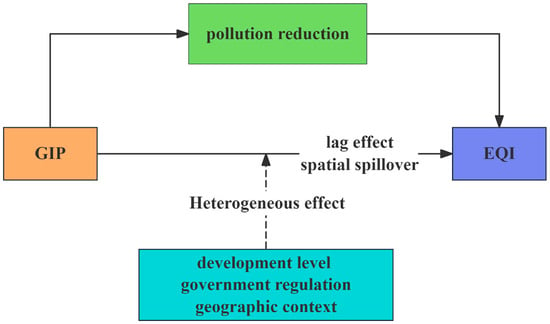
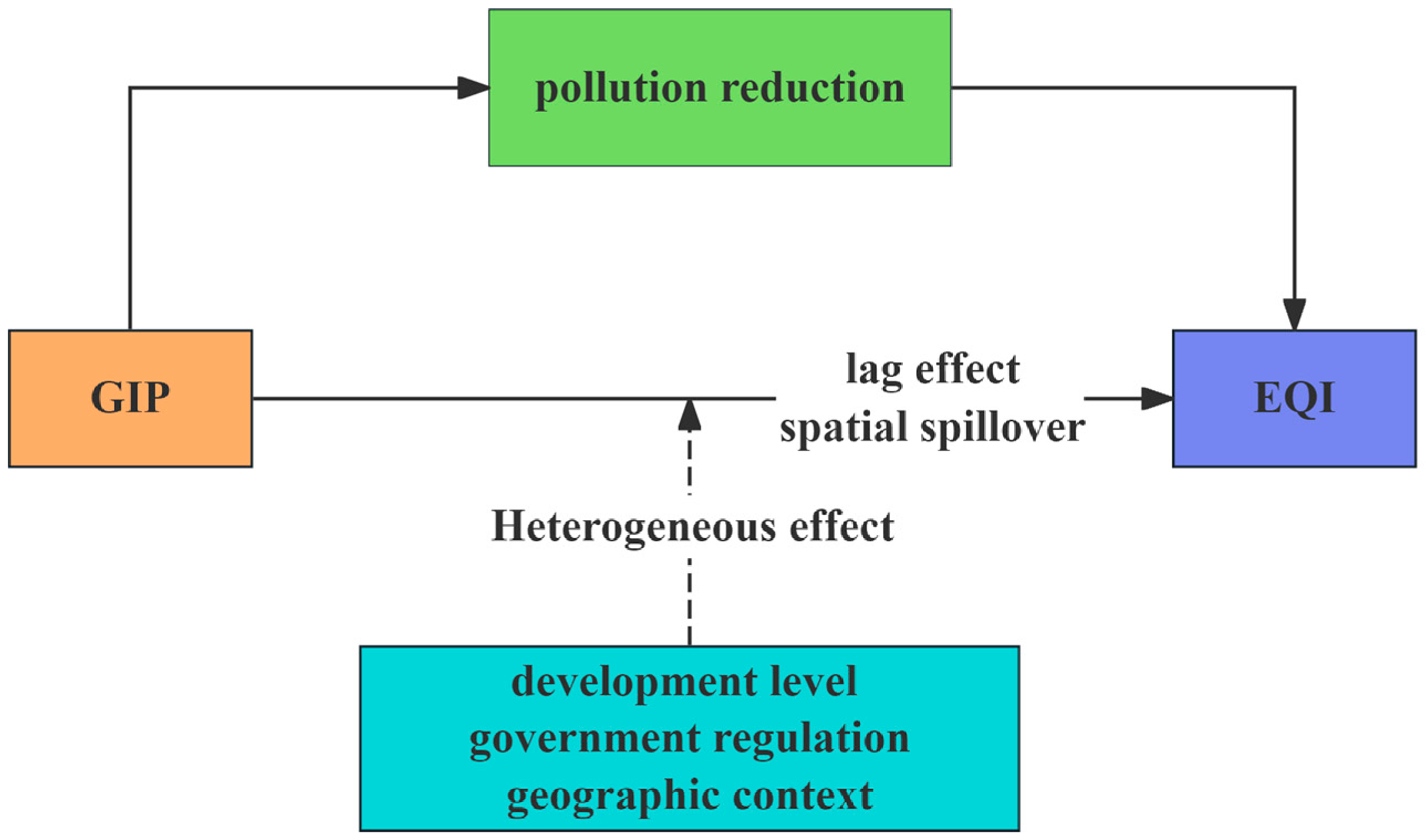
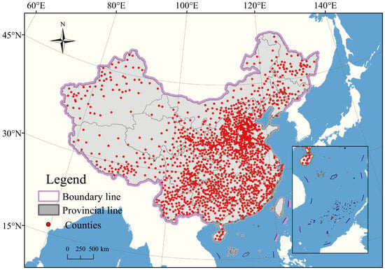
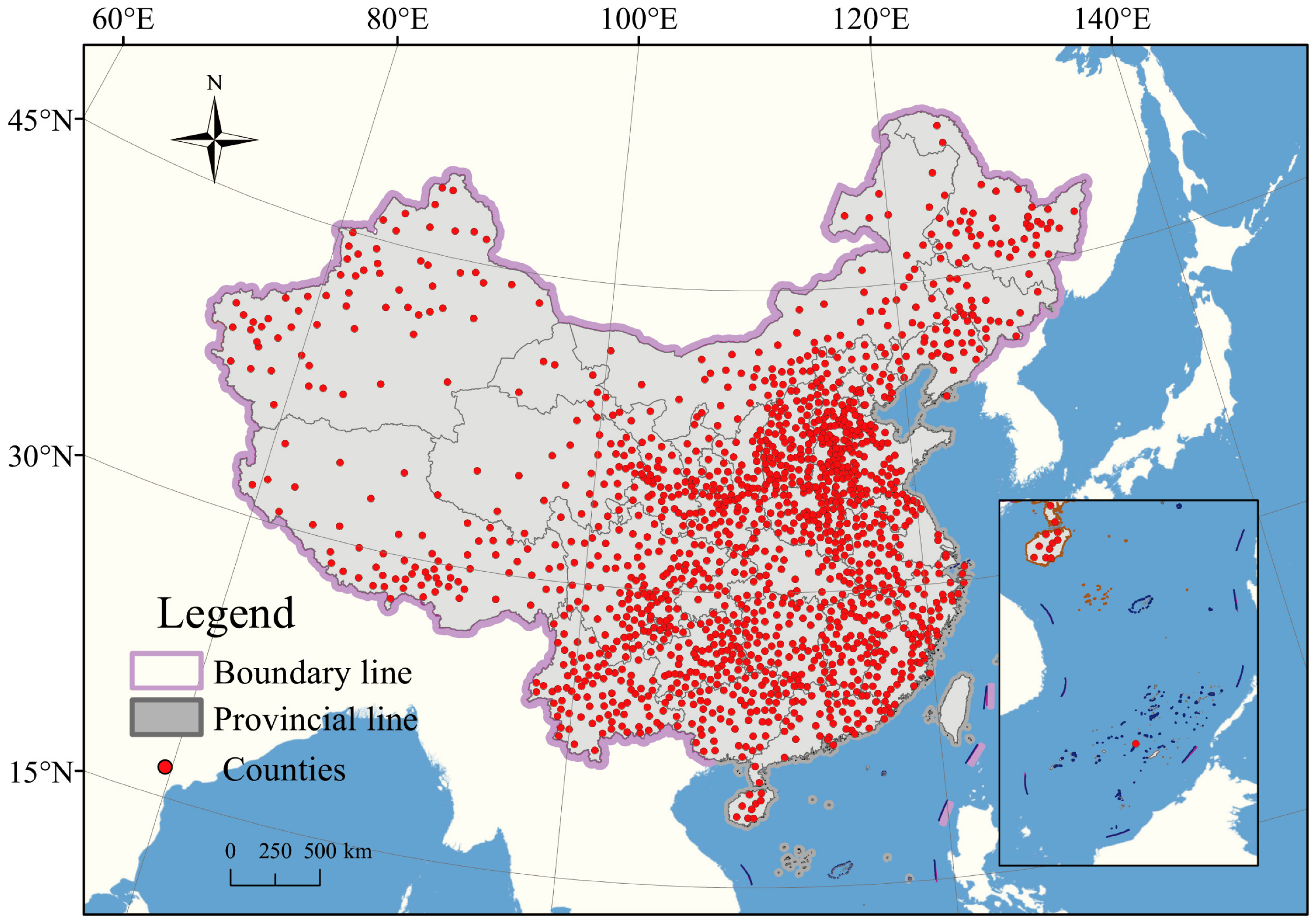
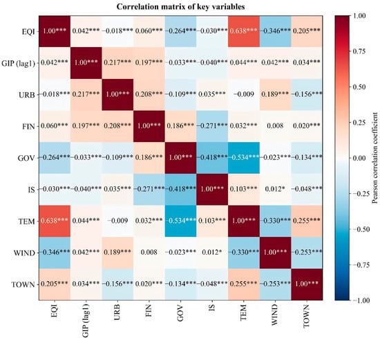
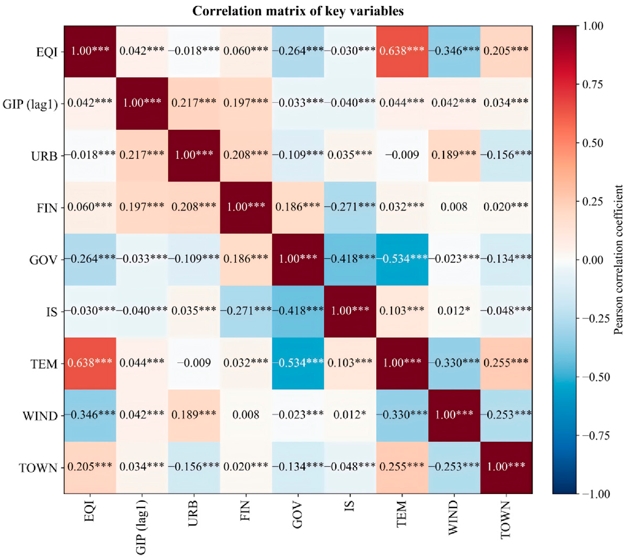
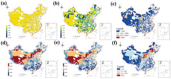
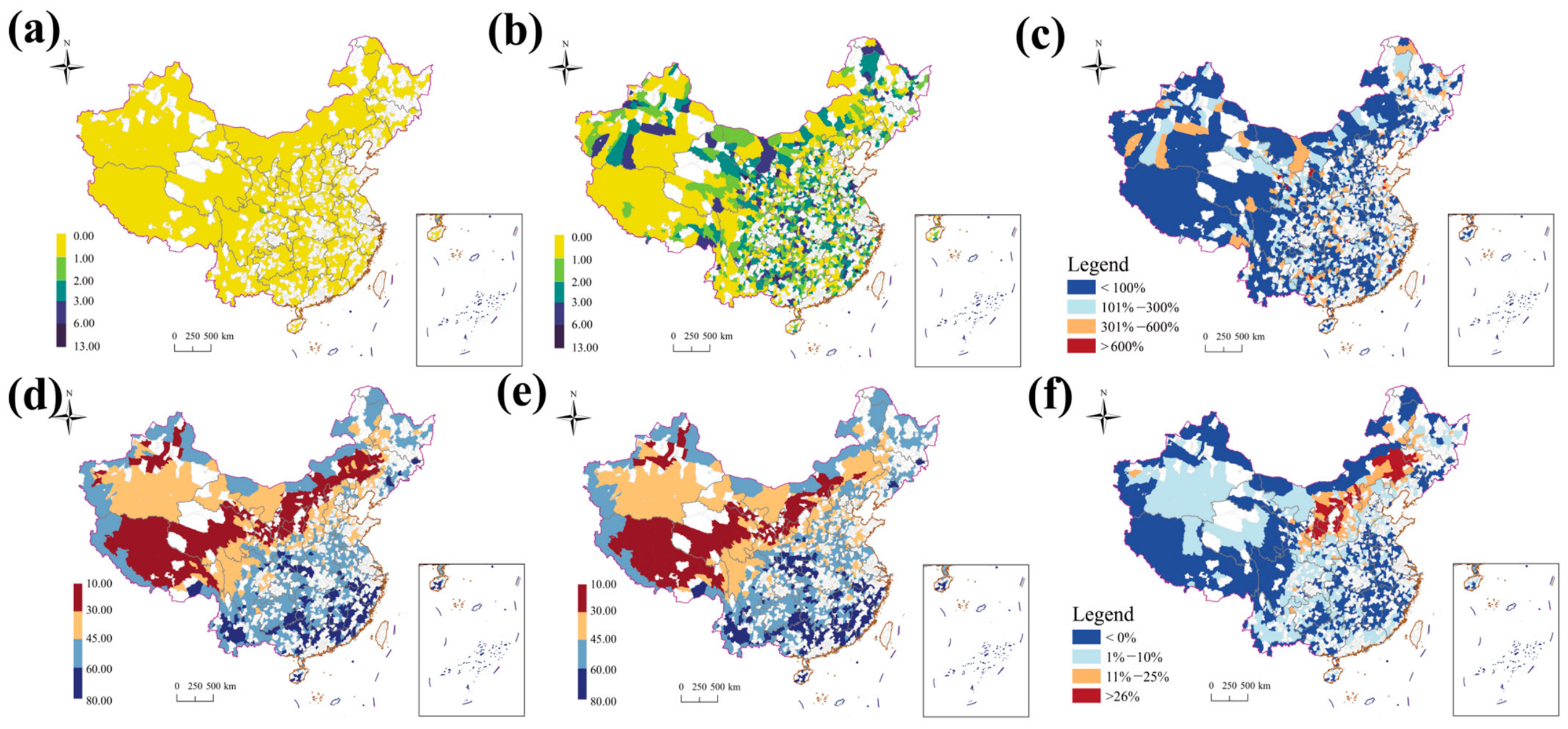
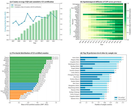
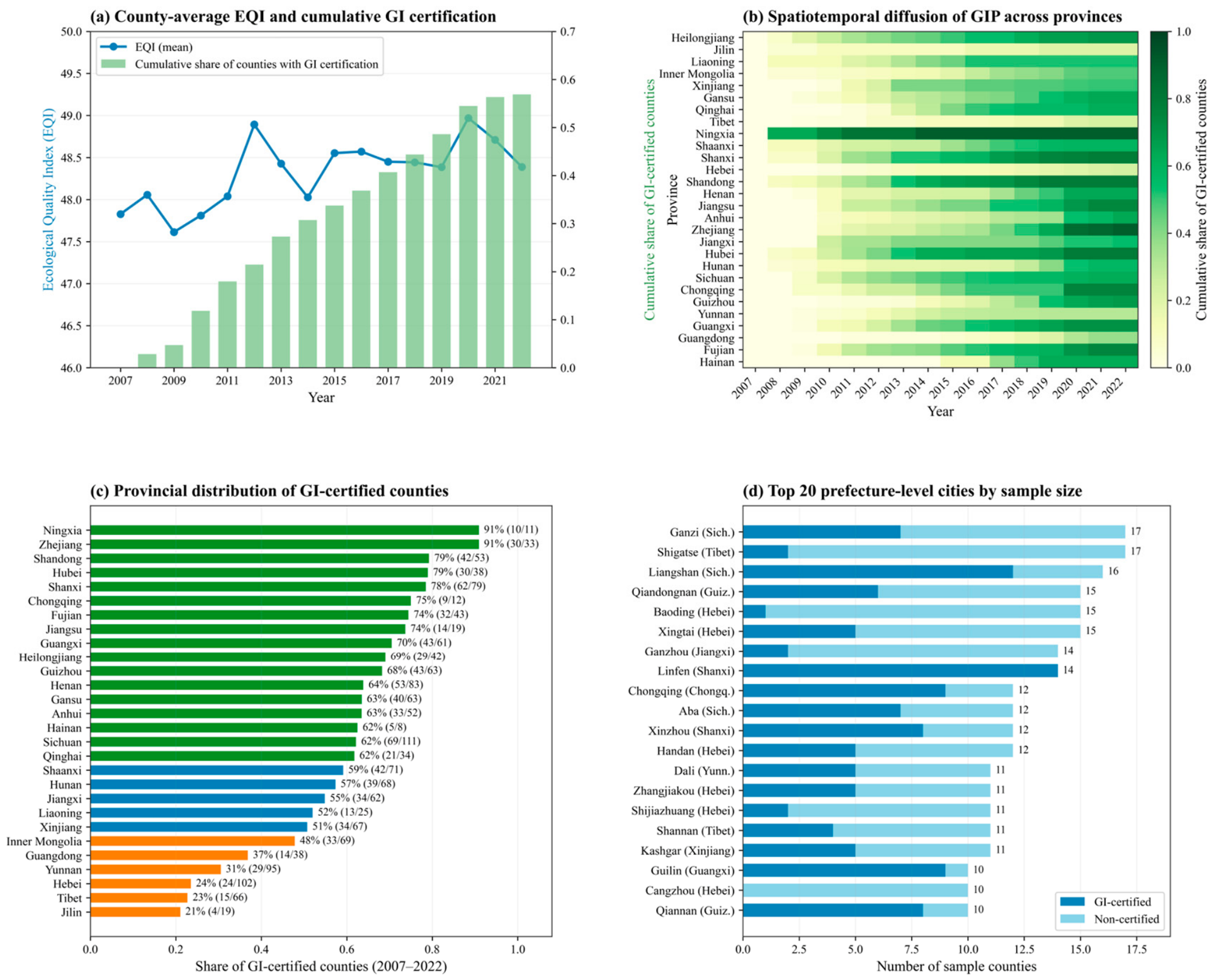
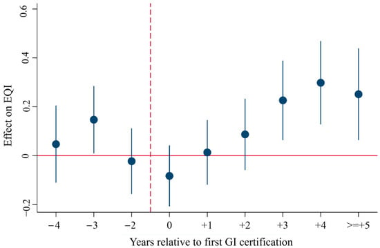
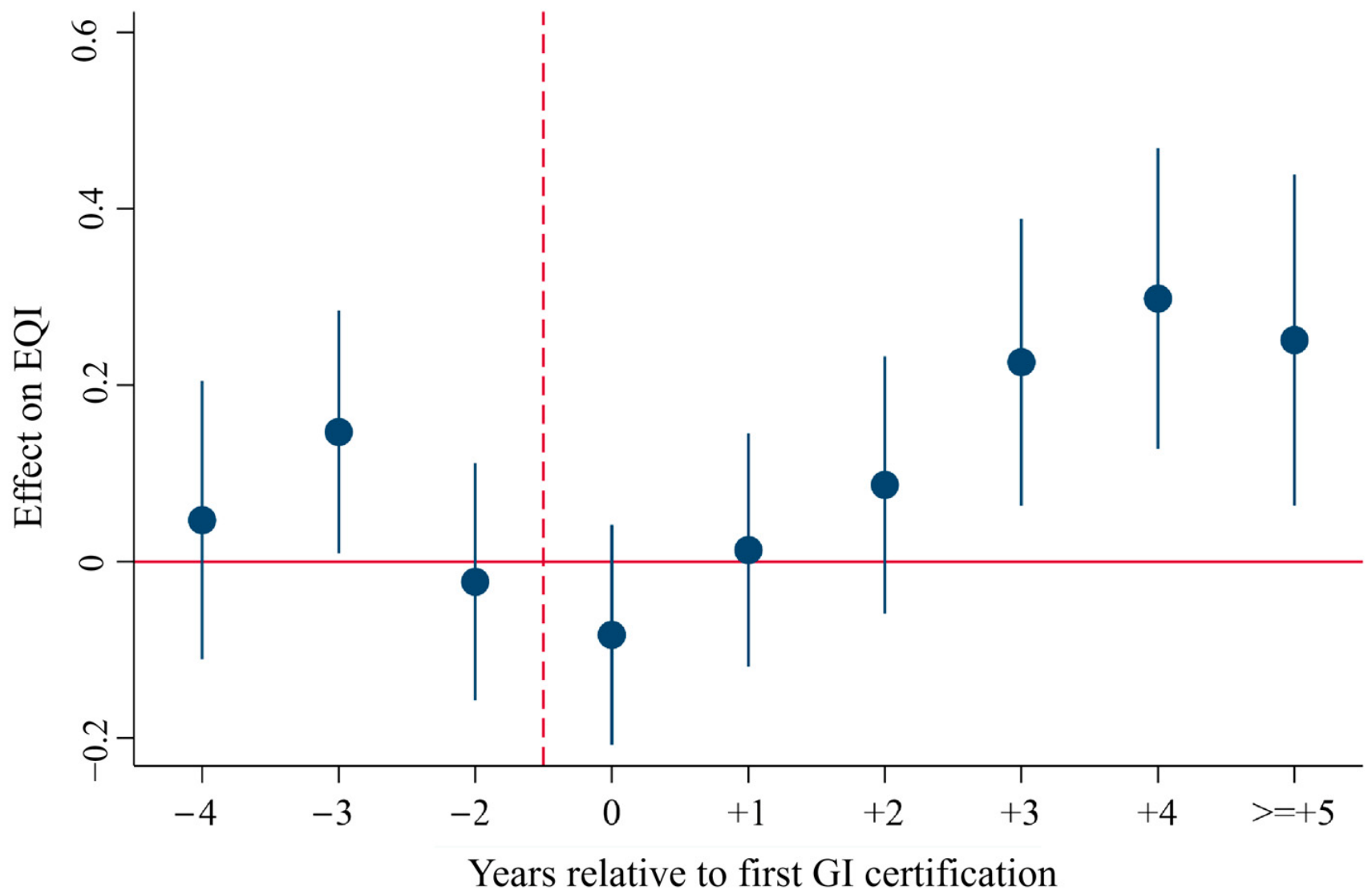
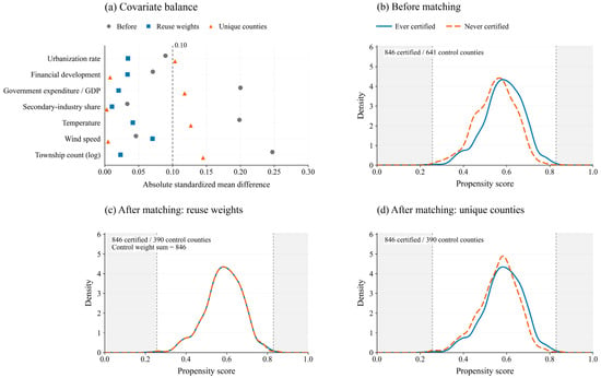
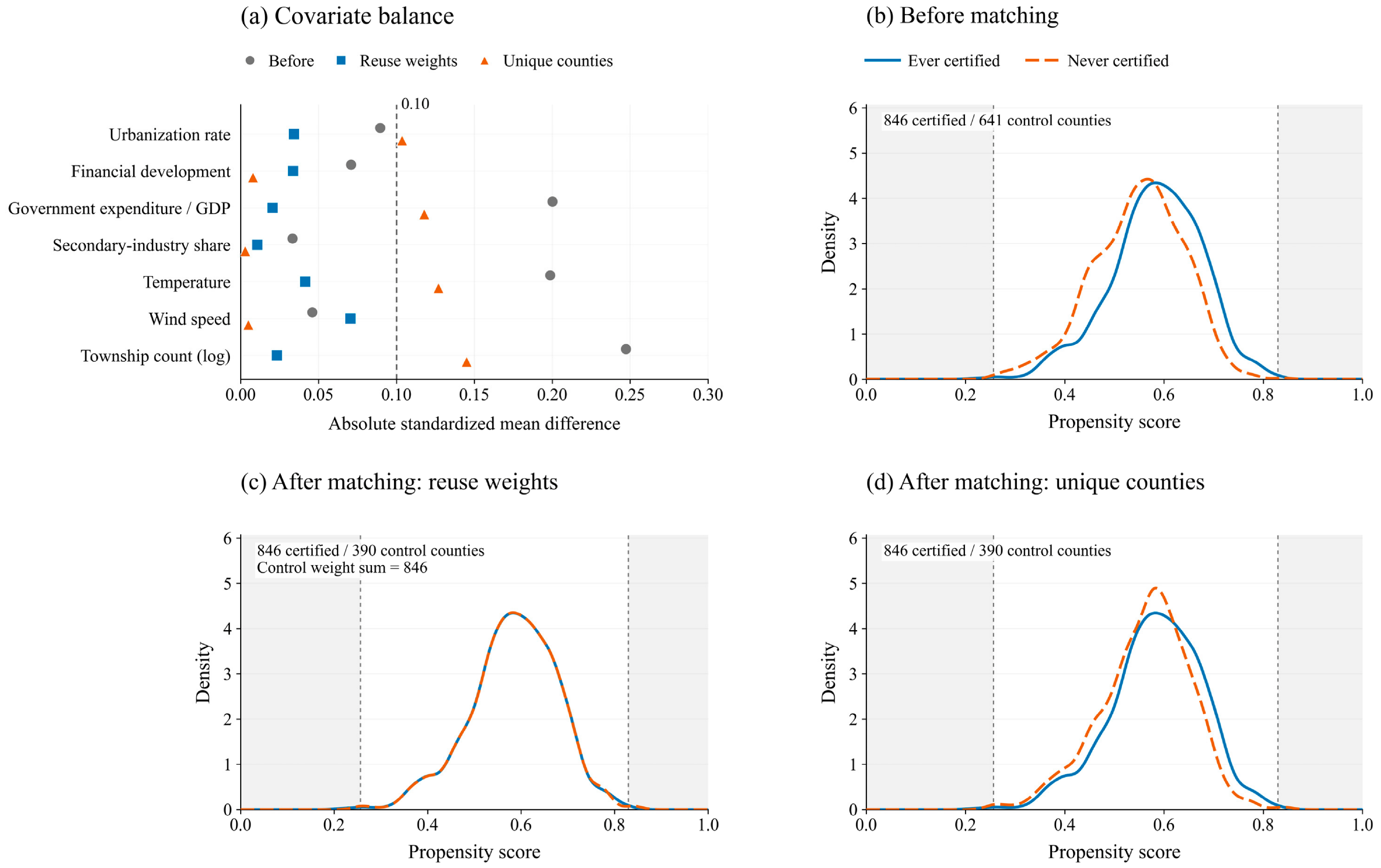
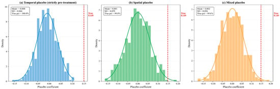
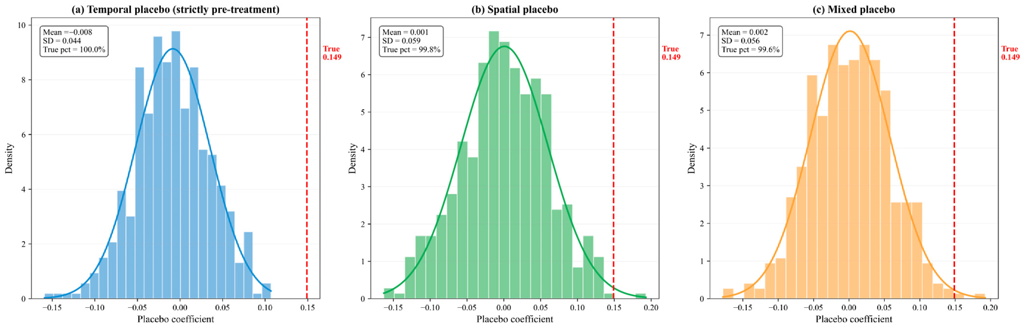
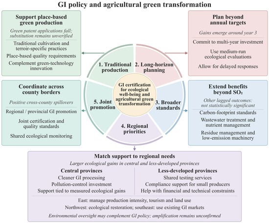
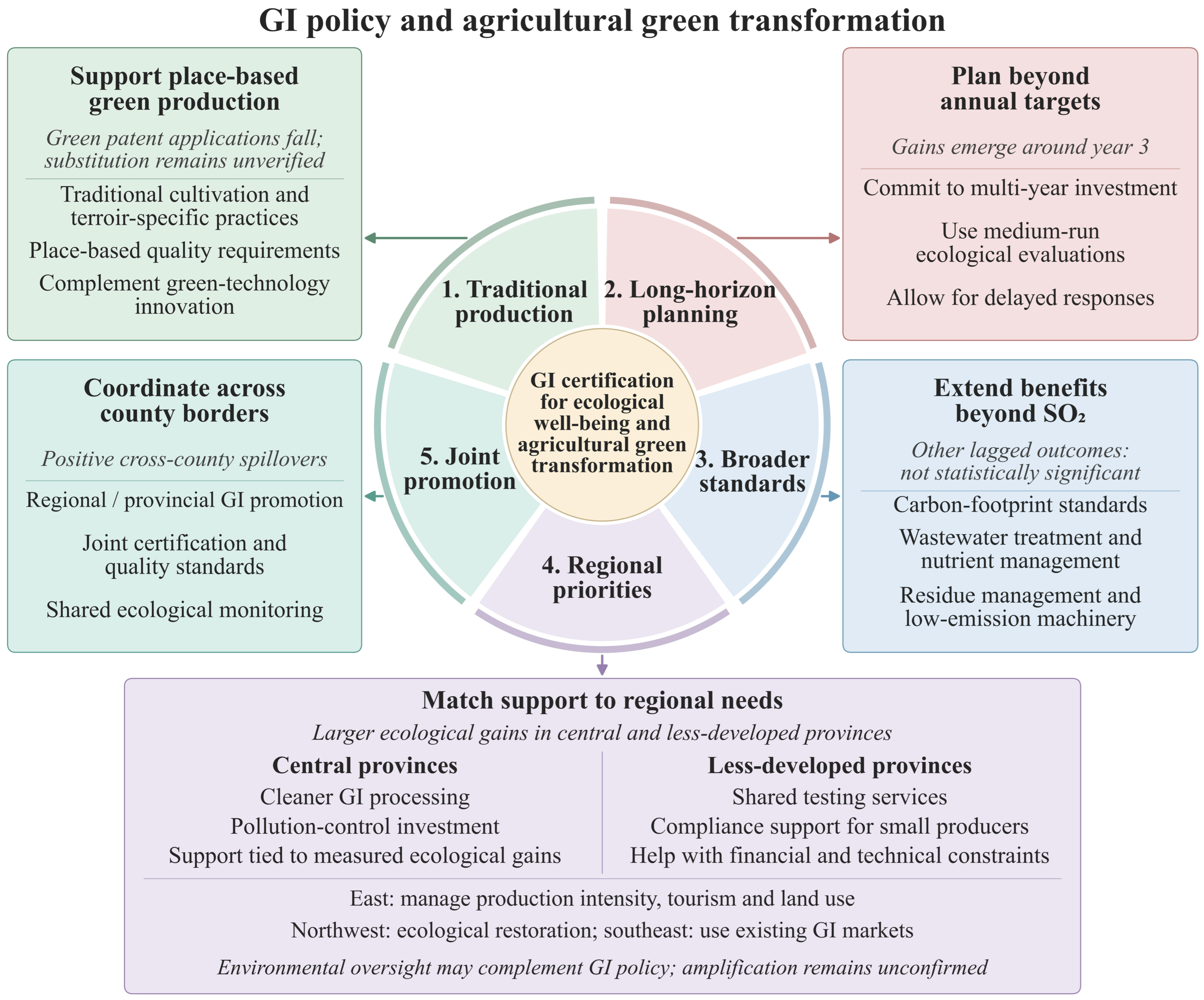

Disclaimer/Publisher’s Note: The statements, opinions and data contained in all publications are solely those of the individual author(s) and contributor(s) and not of MDPI and/or the editor(s). MDPI and/or the editor(s) disclaim responsibility for any injury to people or property resulting from any ideas, methods, instructions or products referred to in the content. |
© 2026 by the authors. Licensee MDPI, Basel, Switzerland. This article is an open access article distributed under the terms and conditions of the Creative Commons Attribution (CC BY) license.