


Abstract
Tea plant leaf nitrogen (N) status directly determines tea yield and quality, and hyperspectral remote sensing enables non-destructive monitoring of these N traits. However, targeted mining of N-sensitive hyperspectral features and interpreting their roles in monitoring models are crucial for achieving stable, year-round tea plant growth monitoring and precision management. To address this, this research proposed a method based on continuous wavelet transform and harmonic decomposition to extract N-sensitive hyperspectral features. Furthermore, interpretable machine learning was employed to elucidate the explicit contributions of these hyperspectral features, thereby establishing a year-round quantitative monitoring model for tea plant N nutrition. Canopy hyperspectral reflectance data (R) of tea plants was collected from 2022 to 2024 concurrently with measurements of leaf N accumulation (LNA). Wavelet features (WF) and harmonic components (HC) were extracted from the hyperspectral data using the continuous wavelet transform and harmonic decomposition, respectively. Multiple machine learning algorithms were employed to fuse multiple categories of sensitive features to establish quantitative monitoring models for LNA in tea plants, with SHapley Additive exPlanations (SHAP) analysis further applied to decode the decision-making mechanism by quantifying individual feature contributions. The results indicated that WF (r = 0.35–0.51) and HC (r = 0.48–0.78) exhibited higher sensitivity to LNA compared to R. Three-feature indices (R2 = 0.50–0.72) significantly improved the monitoring accuracy of leaf N status. The convolutional neural network exhibited consistently robust predictive performance for tea plant N accumulation (R2 = 0.70–0.80). SHAP interpretation further revealed that the core spectral features driving LNA maintained a consistent positive impact across all seasons, with MNDSI(C5, B8) in spring, MMTCI(C51, A2, B126) in summer (mean absolute SHAP = 2.653), and MDCNI(φ10, φ4, φ197) in autumn making dominant contributions. Meanwhile, model-based spatial mapping revealed spatiotemporal heterogeneity (CV = 17.16–31.07%) in N accumulation status across two representative tea plantations. This study establishes a technical framework to quantify the N nutrition status of tea plants, enabling precise, site-specific management and targeted nutrient diagnosis.
1. Introduction
The tea plant ranks among the most vital economic crops within global agriculture. Since tea is a leaf-harvested crop, the accumulation of nitrogen (N) in its leaves critically determines growth, nutritional quality, and ultimate economic value [1]. Consequently, quantifying leaf N levels non-invasively, dynamically and in real time is vital for precision management throughout the annual growth cycle.
Advancements in remote sensing technologies have significantly enhanced the capacity for rapid and quantitative monitoring of crop physiological status. Among these, canopy hyperspectral remote sensing, an important component of modern Earth observation, has gained widespread application due to its ability to capture fine-resolution spectral data related to plant physiology [2]. Traditional approaches primarily rely on raw reflectance (R) data and predefined hyperspectral indices. For instance, Corp et al. [3] assessed maize N uptake under different N levels and compared the performance of various spectral indices. Similarly, Chen et al. [4] developed the double-peak canopy N index (DCNI) for estimating N concentration in wheat and maize, and Li et al. [5] proposed the optimized triangular vegetation index for aboveground N uptake monitoring in winter wheat. However, the relationship between R and crop N levels is characterized by substantial complexity and nonlinearity, limiting the predictive power of models built solely on R. Furthermore, the predefined wavelengths of existing indices are typically optimized for other crops such as wheat and rice, rendering them inadequate for capturing the unique structural traits of perennial tea canopies [6]. This restricts their broader application for tea plant N monitoring. To address these limitations, spectral transformation techniques offer additional pathways for mining hidden physiological information. The continuous wavelet transform enables multi-scale decomposition of hyperspectral curves, enhancing subtle spectral variations associated with plant biochemical status, as demonstrated by Li et al. [7] in winter wheat N estimation models. Moreover, harmonic decomposition can extract stable components linked to plant structural and biochemical traits. Previous studies have shown its efficacy in enhancing anomaly detection in hyperspectral imagery [8] and achieving superior accuracy in potato growth and yield prediction models [9]. Nevertheless, despite the continuous wavelet transform being effective in enhancing subtle spectral variations, these techniques have primarily been utilized in isolation. Specifically, the integration of these multi-domain features at the modeling level through the construction of novel hyperspectral indices derived separately from wavelet and harmonic domains has not been fully explored for mitigating complex canopy interference in the multi-season monitoring of tea plants.
Quantitatively characterizing the relationships between tea plant N indicators and sensitive spectral features is essential for establishing robust monitoring models. With recent advances in artificial intelligence, machine learning approaches have shown strong potential for crop growth monitoring by integrating multi-source spectral information. Silva et al. [10] have demonstrated that random forest (RF) regression performs well in predicting crop N content using hyperspectral data. Nevertheless, conventional machine learning algorithms, including RF and linear models, often exhibit distinct limitations when applied to the season-dependent canopy of perennial tea plants [11]. Fundamentally, these conventional methods rely on shallow learning architectures that process features in a relatively isolated or sequential manner (e.g., the recursive orthogonal partitioning of RF). This shallow mechanism struggles to systematically capture the deep, high-order synergistic interactions required to decouple complex canopy structural variations from true biochemical N signals across different seasons. To overcome these limitations, deep learning offers a more robust framework capable of hierarchical feature abstraction. For example, Yu et al. [12] successfully applied deep learning regression models to estimate leaf N concentration in rapeseed. Despite this potential, the integration of advanced multi-domain hyperspectral feature mining with deep learning architectures remains largely unexplored for tea plant N monitoring. Existing deep learning models in agricultural remote sensing predominantly rely on R or single-domain empirical indices as inputs. Undertanding how to effectively design a deep learning framework to autonomously fuse multi-domain features represents a critical knowledge gap. Bridging this gap is essential to inherently capture the complex, non-linear synergies required for precise multi-season canopy monitoring. However, as deep learning models become increasingly complex to accommodate such multi-domain feature fusion, their inherent “black-box” nature becomes a critical concern. This opacity can obscure variable contributions and decision-making processes, increasing the risk that high accuracy reflects spurious site- or season-specific patterns rather than agronomically meaningful spectral mechanisms [13]. Explainable artificial intelligence methods, particularly SHapley Additive exPlanations (SHAP) analysis, have therefore become widely used to quantify feature contributions and reveal model decision processes. Zhong et al. [14] demonstrated that SHAP analysis can effectively quantify wavelength contributions and explain differences in CNN predictive performance between full-spectrum and feature-spectrum models for soil N estimation. More recently, Wu et al. [15] integrated SHAP analysis with an attention mechanism to dynamically characterize spectral feature importance while enhancing prediction accuracy and interpretability in agricultural spectral analysis. These findings indicate that SHAP analysis provides a useful framework for identifying influential spectral variables and improving the transparency of data-driven prediction models. However, in previous tea-related studies, it remains an unsolved issue how diverse spectral features dynamically drive N estimation models across different seasonal stages. Thus, using SHAP analysis to explicitly evaluate the season-specific contributions of multiple types of sensitive features extracted from hyperspectral data represents a valuable avenue for advancing robust tea plant N monitoring.
Given that the tea plant is a perennial crop, acquiring seasonal N data during different seasonal stages enables real-time assessment of nutrient dynamics and provides a scientific basis for optimizing fertilization strategies. Year-round monitoring also helps identify potential metabolic imbalances at an early stage, allowing timely adjustments to improve both yield and quality. Accordingly, the specific objectives of this study were to (1) identify hyperspectral signatures responsive to N accumulation in tea plants by leveraging the continuous wavelet transform and harmonic decomposition; (2) establish a deep learning model integrating diverse spectral indices to monitor N accumulation; (3) interpret the developed model using the SHAP method to evaluate the season-specific contributions of key spectral features to N estimation; (4) perform a spatiotemporal assessment of N dynamics within tea plants across different seasonal stages.
2. Materials and Methods
2.1. Experimental Design
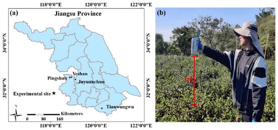
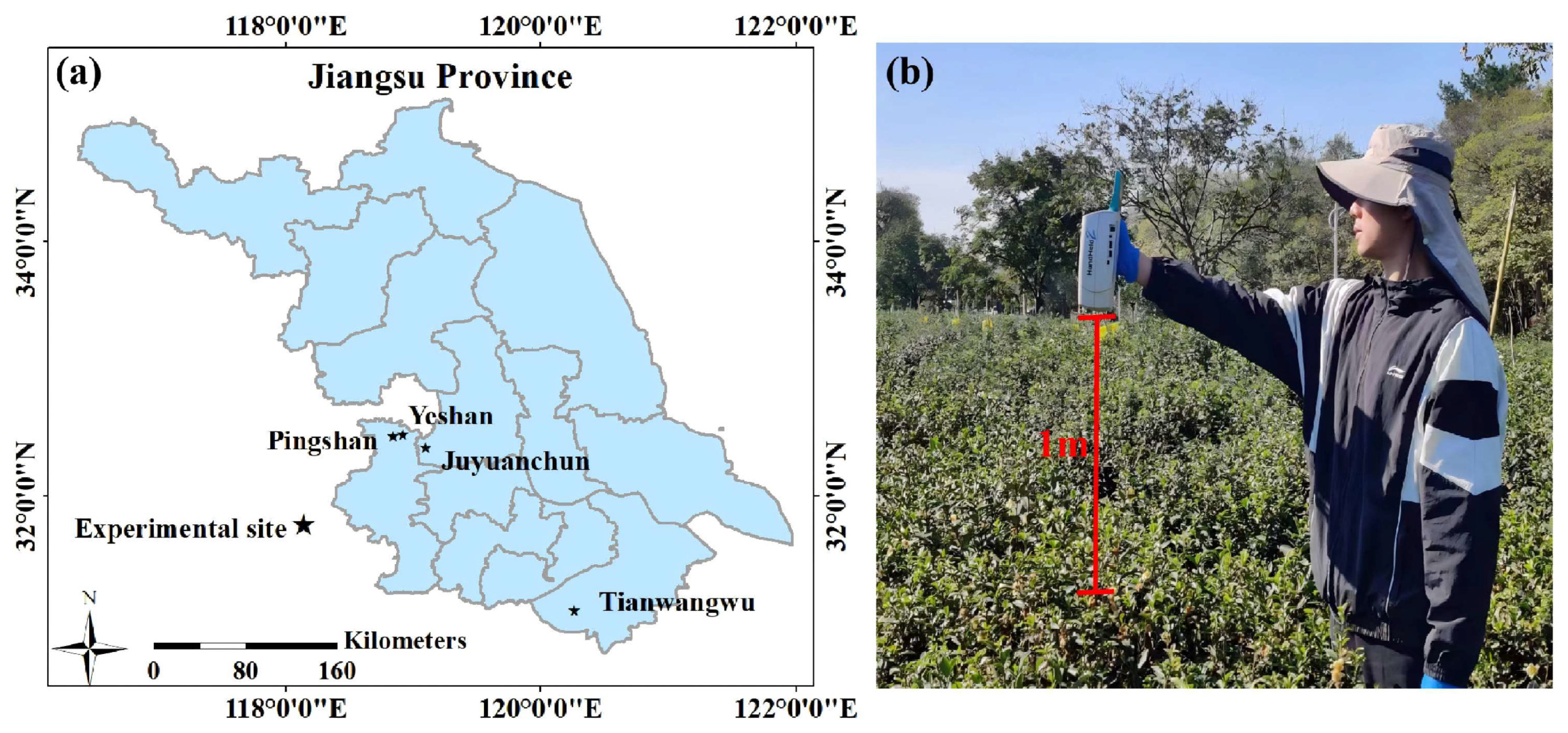
Field experiments were conducted from 2022 to 2024 across four tea gardens in Jiangsu Province, China (Figure 1a), to collect hyperspectral datasets and plant samples. The study area spans an agrometeorological and pedological gradient. Specifically, the Pingshan (32.45° N, 118.81° E) and Yeshan (32.51° N, 118.91° E) sites in Luhe District, Nanjing, together with the Juyuanchun (32.33° N, 119.05° E) site in Yizheng, Yangzhou, are located in the Jianghuai hilly region. These three sites are characterized by slightly acidic yellow-brown soils (pH 5.5 to 6.5) and a north subtropical monsoon climate (mean annual temperature: 15.1 to 16.0 °C; mean annual precipitation: 1000 to 1100 mm; frost-free period: 220 to 237 days). The fourth site, Tianwangwu (31.13° N, 120.28° E) in Wuzhong District, Suzhou, is situated within the Taihu Lake basin. This site features acidic red-yellow soils and a comparatively warmer, more humid microclimate (mean annual temperature: 16.4 to 17.2 °C; mean annual precipitation: >1100 mm; frost-free period: 251 days). Tea plants across all locations were 15 to 30 years old. N fertilization followed the guidelines of local agricultural extension agencies, with an annual application rate of approximately 300 kg N ha−1. To capture the spatial variability of canopy growth characteristics, a spatially balanced random sampling strategy was implemented across the plantation. While strict fixed intervals were not enforced, sampling points were allocated among every individual tea field to ensure comprehensive spatial representativeness (Table 1). In total, 22 measurement campaigns were conducted across the spring, summer, and autumn seasons of 2022 and 2024, yielding a comprehensive dataset of 430 samples (178 in spring, 160 in summer, and 92 in autumn). Detailed survey dates and specific sample sizes for each plantation are comprehensively summarized in Table 1 to demonstrate the adequate representation of target conditions. To rigorously evaluate the generalizability of the proposed models, datasets acquired from the Pingshan and Yeshan sites were designated for model calibration and internal validation, whereas the in situ measurements from the Juyuanchun and Tianwangwu sites were reserved exclusively as an independent test set. Ultimately, consolidating data across these diverse environmental conditions provided a robust foundation for evaluating the tea N monitoring models.
Figure 1.
The study sites and spectral data collection method.
Table 1.
Basic information on the field experiments in this study.
2.2. Hyperspectral Data Collection
Canopy spectral reflectance was measured using an ASD HandHeld 2 spectrometer (ASD Inc., Boulder, CO, USA; 325–1075 nm range, 1 nm interval). The sensor probe was mounted at a 1 m height in a nadir orientation relative to the tea canopy (Figure 1b). Given the instrument’s 25° field of view, the measurement footprint was fully contained within the 50 × 50 cm sampling frame. Simultaneously, the geographic coordinates of all sampling sites were documented using a K90 RTK-GNSS system (CHCNAV, Shanghai, China). To minimize variations caused by solar zenith angle changes, all field measurements were conducted between 11:00 and 14:00 local time under clear sky conditions with minimal wind disturbance. Standard white-panel calibrations bracketed each target measurement to maintain high reflectance precision. At each observation point, spectral data were collected in triplicate at the exact same position. During data preprocessing, the triplicate measurements were first averaged to derive a representative reflectance spectrum for each site. Because pronounced instrument-related noise was observed at both spectral margins, the averaged spectra were truncated to 400–890 nm. Finally, the retained spectra were smoothed using a Savitzky–Golay filter with a window length of 21 and a third-order polynomial.
2.3. Tea Plant N Status Measurement
Immediately after the hyperspectral measurements, leaf sampling was conducted within 50 × 50 cm quadrats co-located with the spectral acquisition points. Quadrats were positioned based on previous pruning boundaries to ensure that only current-year leaves were collected. Fresh leaf samples were first subjected to enzyme deactivation at 105 °C for 30 min, followed by oven-drying at 85 °C until a constant weight was reached. The total dry matter of the leaf samples was recorded. Subsequently, the dried samples were ground into fine powder and analyzed for leaf N content using a multi EA 5000 elemental analyzer (Analytik Jena, Jena, Germany). Leaf N accumulation (LNA) was calculated using the following formula:
LNA = leaf N content × leaf dry matter
2.4. Hyperspectral Feature Mining Methods
2.4.1. Harmonic Decomposition
Harmonic decomposition models a periodic sequence as the superposition of multiple sine and cosine waves. In this study, hyperspectral data with M bands were mathematically treated as a discrete periodic signal with a period of M. By applying harmonic decomposition, the hyperspectral signature is transformed into a series of harmonic components, thereby revealing intrinsic spectral patterns and relationships among bands. Let a spectral curve composed of M bands be represented as a vector R(k) = (r1, r2, …, rM), where rk denotes the spectral reflectance of the kth band (k = 1, 2, …, M).
The harmonic components (HC) derived from the mth-order harmonic decomposition are computed as
where m (m = 1, 2, 3, …) denotes the order of the harmonic decomposition and corresponds to an integer multiple of the fundamental frequency. A0/2 represents the mean spectral reflectance and Cmsin(2πmk/M + φm) is the mth-order HC. The parameters Am, Bm, Cm and φm represent the cosine amplitude, sine amplitude, harmonic amplitude and harmonic phase, respectively, of the mth-order harmonic. In this study, the harmonic decomposition was performed on the full spectral range comprising 490 bands. In this study, the harmonic decomposition was initially performed on the full effective spectral range comprising 490 bands (400–890 nm), treating it as a discrete periodic sequence of length 490. Because the resulting harmonic variables exhibit axial or central symmetry, the components beyond order 245 generate mathematically redundant information relative to the first half. Therefore, to eliminate redundancy while preserving all independent spectral features, only the first 245 harmonic orders were retained, resulting in exactly 245 distinct variables for each HC type (Am, Bm, Cm and φm) for subsequent index construction.
φm = tan−1(Am/Bm)
2.4.2. Continuous Wavelet Transform
The continuous wavelet transform offers multi-scale decomposition capabilities, enabling the precise capture of subtle spectral features associated with biochemical content. Moreover, the resulting wavelet features (WF) maintain a direct correspondence with the raw reflectance bands, thereby enhancing interpretability. Specifically, WF are extracted by convolving a scaled and translated mother wavelet function with the reflectance spectra. The transformation is defined by the following formula:
In the formulation, ψ(k) represents the mother wavelet function, with the Mexican hat (mexh) wavelet selected for this research. ψs,λ(k) denotes the scaled and translated mother wavelet function, where s is the scaling factor (specifically set to scales 3, 4, 5, and 6) and λ is the translation factor, expressed in units of wavelength. The resulting wavelet coefficient, denoted as wf(s, λ), quantifies the similarity between the mother wavelet function and the reflectance spectrum at a specific scale s and translation λ.
In this study, raw spectra (400–890 nm) were decomposed using the continuous wavelet transform to thoroughly explore latent information embedded in the hyperspectral data. Correlation analyses were conducted between the WF at different scales and the N accumulation value of tea leaves, and the scale exhibiting the strongest correlation was identified as the optimal scale. A key advantage of this approach lies in its robust time–frequency localization capability. By applying the mother wavelet function across a range of scales, raw spectral signals were decomposed into multi-scale components, enabling the fine separation and enhancement of subtle spectral absorption features associated with LNA. Since the transformation process covered the entire spectral range, the resulting WF preserved comprehensive spectral information, facilitating the extraction of the most sensitive features from a multi-scale perspective.
2.5. Constructing Novel Hyperspectral Indices for Tea Plant N Monitoring
Based on the acquired hyperspectral datasets, raw spectral bands within the 400–890 nm range with a high signal-to-noise ratio and minimal noise were selected for index construction. Using the exhaustive search method, six novel spectral indices were developed, including three two-feature indices—modified difference spectral index (MDSI), modified normalized difference spectral index (MNDSI), and modified ratio spectral index (MRSI)—and three three-feature indices—modified double-peak canopy N index (MDCNI), modified MERIS terrestrial chlorophyll index (MMTCI), and modified red-edge normalized difference index (MNDindex). The complete list of all indices and their corresponding formulas is provided in Table 2. Single-feature, two-feature, and three-feature indices were constructed using three types of hyperspectral data sources: R, WF, and HC. For each data source, the top 30 index combinations with the highest correlations with N accumulation were selected to generate four feature index datasets: the R feature index dataset (RFI), the WF feature index dataset (WFFI), the HC feature index dataset (HCFI), and a hybrid feature index dataset (HFI) integrating all three sources. Subsequently, predictive models were constructed and systematically evaluated based on these four feature index datasets.
Table 2.
Hyperspectral indices selected for this study.
2.6. Model Construction via Explainable Deep Learning Algorithms
To develop the predictive model aimed at quantifying N accumulation in tea plants, this study implemented two machine learning algorithms and one deep learning architecture. The machine learning algorithms included random forest (RF) and least absolute shrinkage and selection operator (LASSO), while the deep learning algorithm was a convolutional neural network (CNN). Regarding the RF model, the number of candidate variables considered at each split (mtry) was systematically optimized across a range from 1 to the total feature count, while the ensemble size (ntree) was evaluated at discrete intervals of 500, 1000, 1500, and 2000. For the LASSO model, the mixing parameter (α) underwent fine-tuning between 0 and 1 with a precise step size of 0.001, with the regularization penalty (λ) held constant at 0.1. In this study, a one-dimensional convolutional neural network (1D-CNN) integrated with residual connections was developed to estimate tea LNA from the calculated spectral index datasets. Because the inputs comprised discrete spectral indices rather than continuous wavebands, these indices were concatenated and reshaped into a 1D feature array (structured as batch size, channel, number of indices) to serve as the network input. This design allows the convolutional kernels to capture complex, nonlinear combinatorial interactions among different vegetation indices. The core feature extraction module comprises three sequential convolutional blocks with 64, 128, and 256 output channels, utilizing kernel sizes of 5, 5, and 3, respectively. To maintain the dimensional length of the feature array across convolutions, zero-padding was uniformly applied. Each block incorporates a single 1D convolutional layer, a batch normalization layer to stabilize training, and a LeakyReLU activation function (negative slope = 0.1). A max-pooling layer (kernel size = 2, stride = 2) was applied immediately after the first convolutional block to downsample the feature maps and filter redundant index information. To facilitate gradient propagation across the network, 1 × 1 convolutional projections were employed to establish residual connections between successive blocks, ensuring channel alignment for element-wise addition. The final feature representations were aggregated using a global average pooling layer, followed by a dropout layer (rate = 0.5) to mitigate overfitting, and a fully connected output layer mapping the extracted features to a single N accumulation value. Model training was optimized using the AdamW algorithm with an initial learning rate of 5 × 10⁻⁴ and a weight decay of 1 × 10⁻². The Smooth L1 Loss function was selected to robustly penalize prediction errors. The training process was executed with a batch size of 8 for a fixed duration of 120 epochs, utilizing a cosine-annealing learning rate scheduler (Tmax = 120) to smoothly decay the learning rate.
Model performance was evaluated using a 10-fold cross-validation scheme based on datasets from Pingshan and Yeshan. The model exhibiting the highest coefficient of determination (R2), along with the lowest root mean square error (RMSE) and relative error (RE), was selected as the optimal model for accurately monitoring N accumulation in tea leaves. To mitigate the inherent opacity of complex machine learning models, SHapley Additive exPlanations (SHAP) were implemented to quantitatively evaluate individual feature contributions and elucidate the underlying predictive mechanisms. Specifically, a shap.GradientExplainer was constructed to interpret the trained network. First, to establish the reference expectation for the GradientExplainer, a baseline background cohort was constructed. The background sample size was strictly defined as min(100, n) (where n is the total number of samples in the development dataset), resulting in 100, 100, and 72 background samples for the spring, summer, and autumn models, respectively. Independent test data from Juyuanchun and Tianwangwu were strictly excluded from this process. Subsequently, to ensure comprehensive structural interpretation and mitigate localized sampling bias, local feature attributions were calculated across the entire available development dataset (defined as min(200, n)), corresponding to 158, 140, and 72 explanation samples across the three seasons. Subsequently, to ensure comprehensive structural interpretation and mitigate localized sampling bias, local feature attributions were calculated across the entire available dataset rather than a specific subset. To ensure practical agronomic interpretability, the computed raw Shapley values were rescaled back to their original physical dimensions by multiplying them by the standard deviation of the target variable. Concurrently, the standardized feature inputs were transformed back to their real physical values via an inverse scaling procedure. Finally, the global feature importance rankings and their directional impacts on N accumulation were illustrated and evaluated using both SHAP summary dot plots and mean absolute SHAP value bar plots. In addition, the generalizability of the screened optimal model was externally evaluated using independent datasets collected from Juyuanchun and Tianwangwu. A higher R2, coupled with lower RMSE and RE values, indicates better independent validation performance of the model. All data analyses and model constructions were implemented using the Python programming language (version 3.12.0, Python Development Core Team, 2023). Furthermore, graphs and figures were generated using Origin software (version 2024,OriginLab Corporation, Northampton, MA, USA).
where Pi and Oi represent the predicted and actual values, respectively, and n represents the number of samples.
3. Results
3.1. Statistical Analysis of Tea Plant LNA
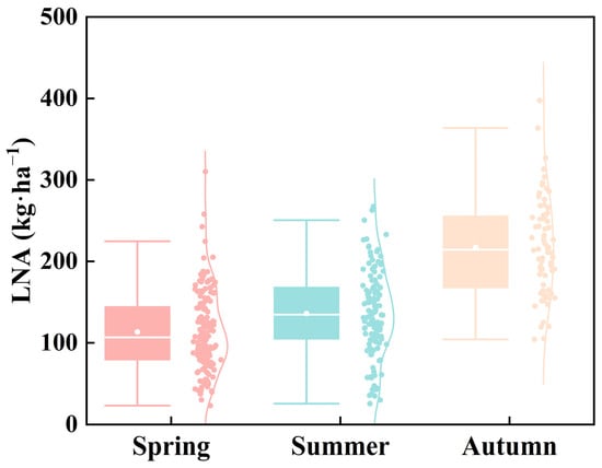
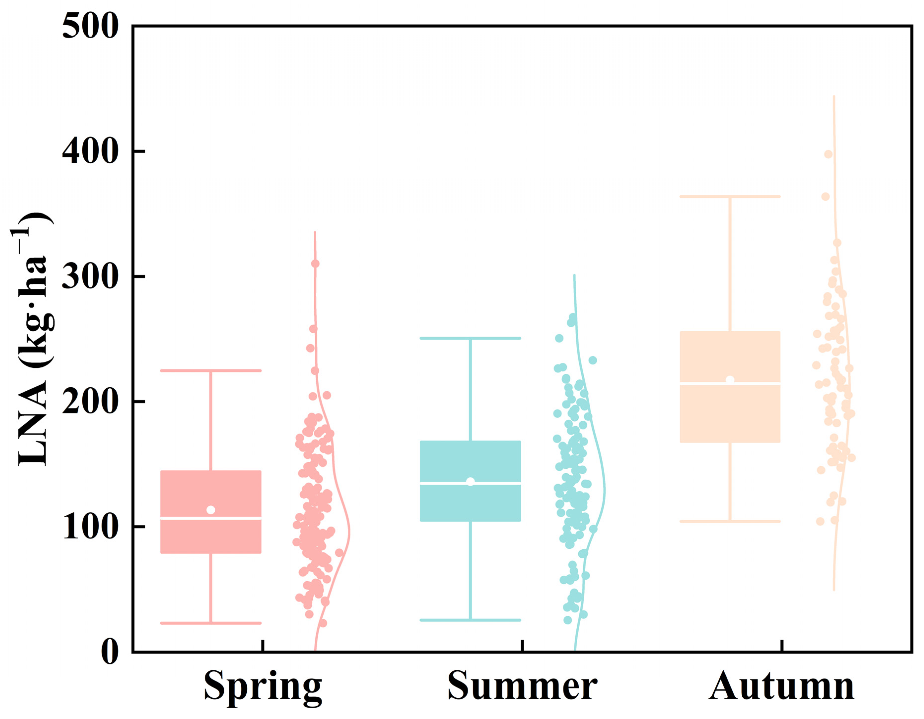
Seasonal dynamics in LNA were analyzed (Table 3, Figure 2), which showed clear descriptive seasonal differences. During spring, LNA varied from 23.27 to 310.32 kg·ha−1. In summer, the corresponding ranges slightly contracted, with LNA ranging from 25.62 to 267.40 kg·ha−1. By autumn, LNA reached its peak levels, with LNA ranging from 104.27 to 397.63 kg·ha−1, indicating substantial biomass accumulation by the end of the growing season.
Table 3.
Descriptive statistics of tea plant leaf LNA during different seasons.
Figure 2.
Tea plant leaf N accumulation (LNA) across three seasons.
3.2. Mining Sensitive Hyperspectral Features of LNA Using Continuous Wavelet Transform and Harmonic Decomposition
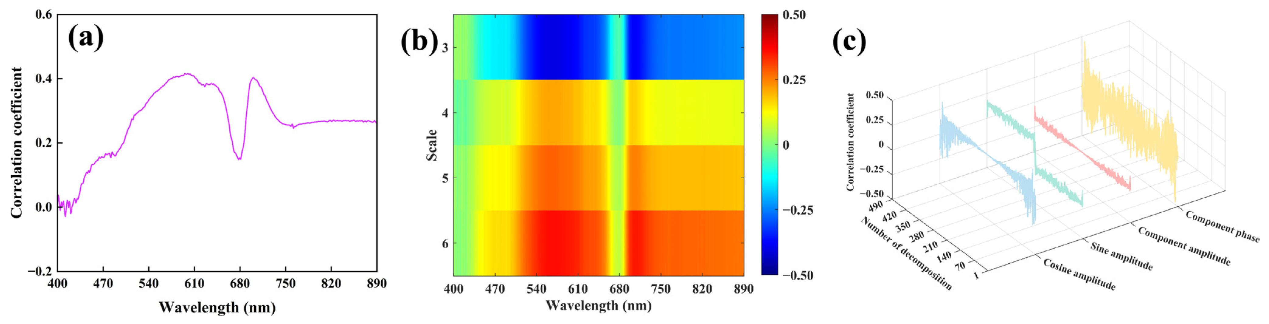
Correlation analyses between tea plant LNA and R across different seasons revealed sensitive wavelengths (Figure 3a). In spring, the strongest correlation for LNA occurred at 595 nm (r = 0.42). The continuous wavelet transform further extracted WF, which were then correlated with the N status (Figure 3b). These WFs showed pronounced scale-dependent variations, and the optimal features were identified based on their maximum correlation strengths with the N parameters. In spring, the WF at 566 nm (scale 6) exhibited the highest correlation with LNA (r = 0.41). Harmonic decomposition generated four types of HC (An, Bn, Cn, and φn), each displaying distinct correlation patterns with the N status (Figure 3c). Notably, φ8 showed a strong relationship with LNA, with a correlation coefficient of 0.76 in spring. The Supplementary Materials contain detailed results on the season-specific sensitive spectral features identified for summer and autumn (Figures S1 and S2).
Figure 3.
Correlation coefficients between leaf N accumulation (LNA) and raw spectral reflectance (R; (a)), wavelet features (WF; (b)), and harmonic components (HC; (c)) in spring.
3.3. Constructing the Spectral Indices Sensitive to Tea Plant LNA
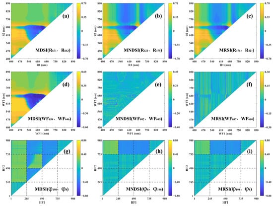
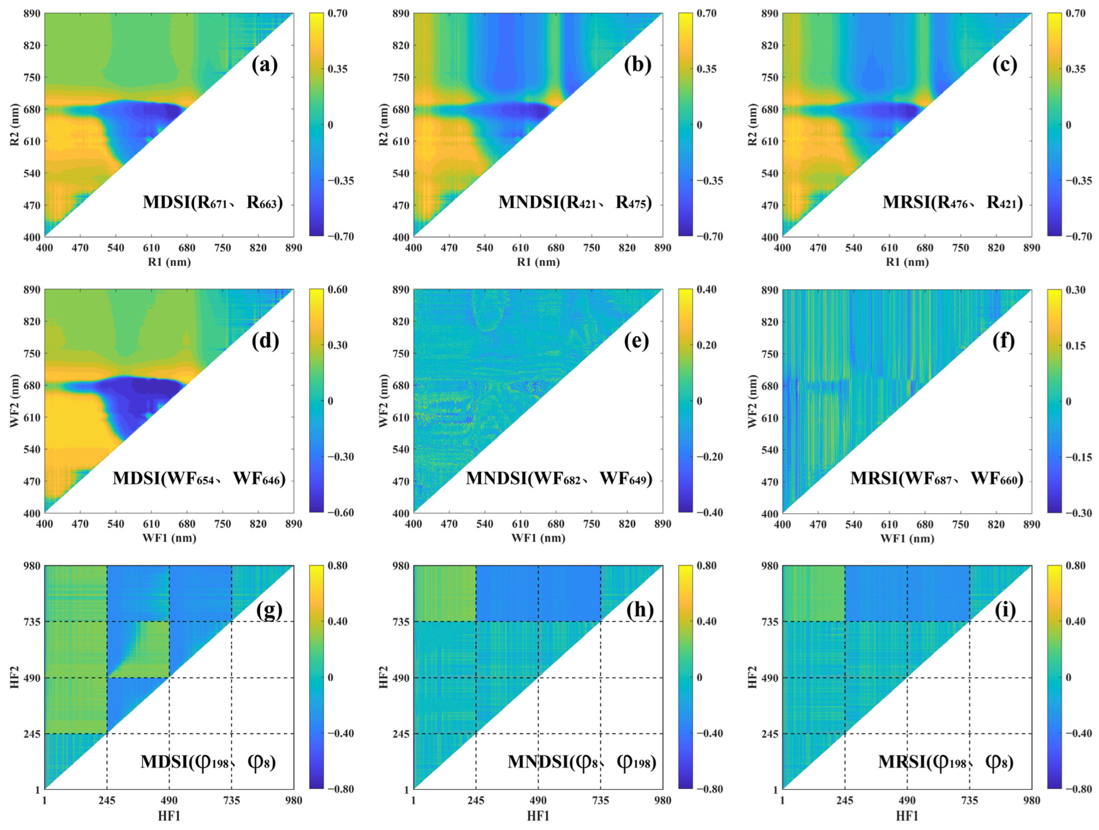
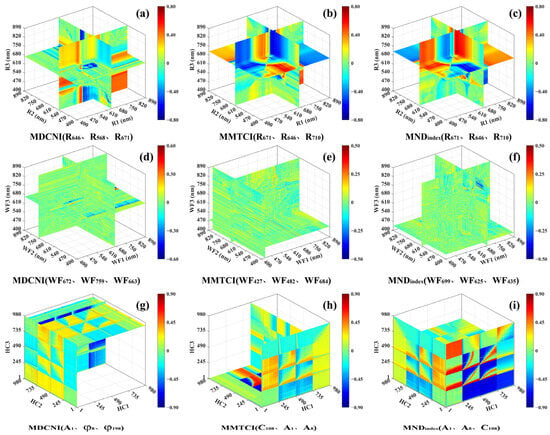
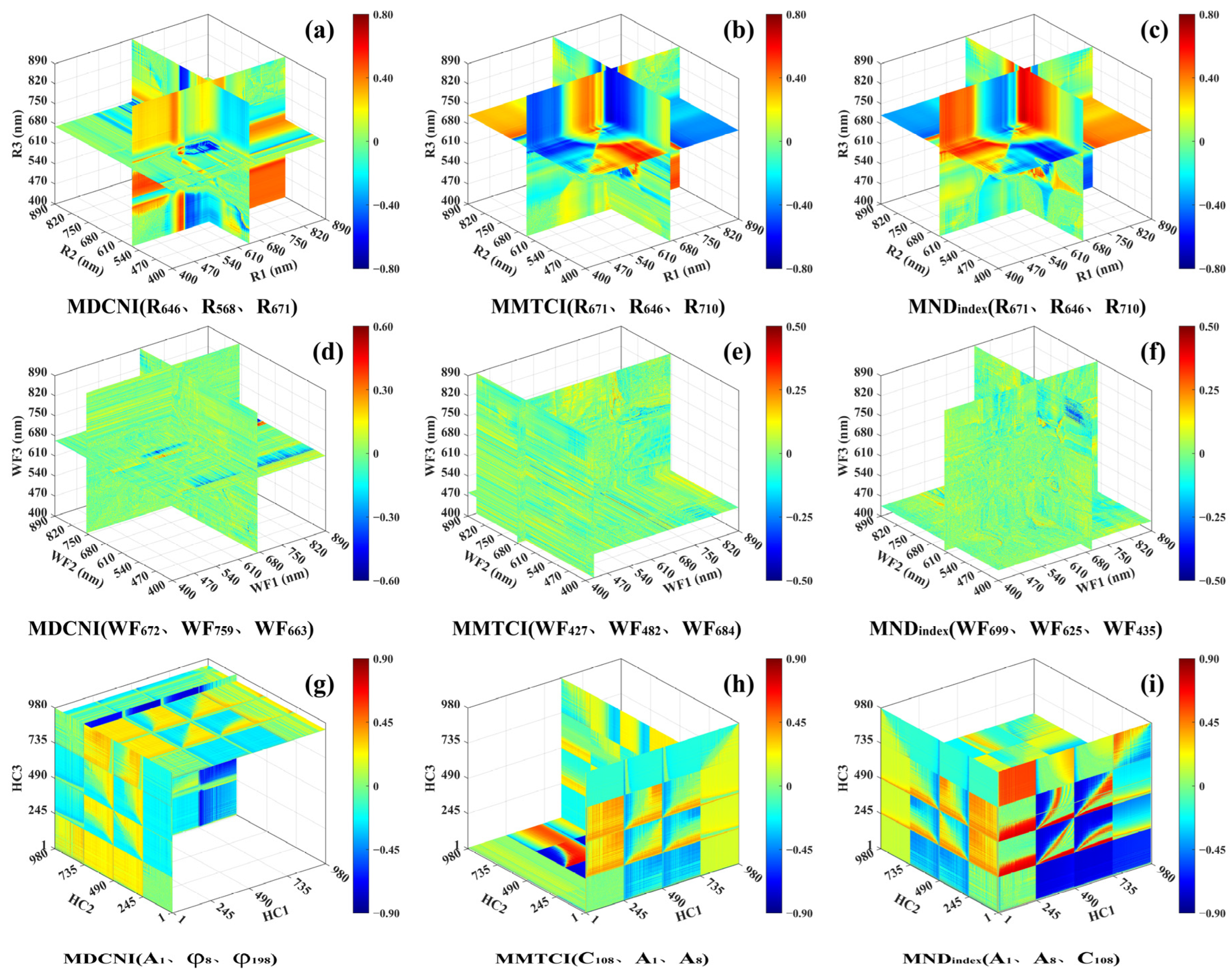
Two-feature and three-feature spectral indices were developed from different feature datasets, and the optimal indices were subsequently selected based on their correlation coefficients. As illustrated in Figure 4 and Figure 5, among the two-feature indices, the most strongly correlated R-based index for LNA was MDSI(R671, R663) (Figure 4 and Figure 5). For indices derived from WF, the highest correlation was observed for MDSI(WF654, WF646). Similarly, correlation analyses between the N status and HC-based indices identified MRSI(φ198, φ8) as the most sensitive for monitoring LNA. The most sensitive R-based three-feature index for LNA was MNDindex(R671, R646, R710), respectively. For WF-derived three-feature indices, the strongest correlation was found for MDCNI(WF672, WF759, WF663) with LNA. Likewise, HC-based three-feature indices revealed MNDindex(A1, A8, C108) as the most sensitive for LNA. These results correspond specifically to the spectral indices identified in spring, while analogous results for summer and autumn are provided in the Supplementary Materials (Figures S3–S6).
Figure 4.
The two–feature spectral indices (MDSI, MNDSI and MRSI) derived from R (a–c), WF (d–f), and HC (g–i) were used to monitor LNA in spring. Note: The values in parentheses in each panel are the selected sensitive feature indices.
Figure 5.
The three–feature spectral indices (MDCNI, MMTCI and MNDindex) derived from R (a–c), WF (d–f), and HC (g–i) were used to monitor LNA in spring. Note: The values in parentheses in each panel are the selected sensitive feature indices.
Based on the identified two-feature and three-feature sensitive indices, linear regression models between tea plant N status and these indices were established across different seasons (Table 4). The results demonstrate that indices derived from WF and HC achieved higher predictive accuracy compared to those based on R. In spring and summer, HC-based two-feature and three-feature sensitive indices yielded higher accuracy for LNA. During autumn, WF-based two-feature indices provided strong predictive accuracy across N indicators, whereas HC-based three-feature indices achieved the highest accuracy for LNA.
Table 4.
The 10-fold cross-validation results of simple linear regression models between optimal hyperspectral indices and tea plant N accumulation across different seasons.
3.4. Construction and Interpretability Analysis of the Machine Learning Model for Tea Plant LNA Monitoring
To systematically compare the performance of different machine learning algorithms in monitoring tea plant LNA, this study independently constructed and evaluated models using RF, LASSO, and CNN. The models were trained on feature index datasets derived from three individual data sources (RFI, WFFI, and HCFI), as well as on an HFI. As shown in Table 5, the feature index dataset constructed from R produced moderate predictive power, with determination coefficients ranging from 0.49 to 0.66. The datasets derived from WFFI performed slightly better, yielding R2 values between 0.50 and 0.64. In contrast, the feature index dataset based on HC showed a marked improvement, reaching coefficients of determination as high as 0.78. The HFI further enhanced prediction accuracy, with R2 increasing to approximately 0.67–0.80. Among the tested algorithms, CNN-based models consistently delivered the highest performance, attaining R2 values up to 0.80, whereas LASSO and RF models reached 0.73 and 0.74, respectively. A seasonal comparison indicated that LNA estimation achieved its best performance in summer. Overall, the model constructed using CNN and the HFI achieved the best performance.
Table 5.
The 10-fold cross-validation results of models for estimating leaf N accumulation (LNA) based on multiple types of spectral information using different algorithms in different seasons.
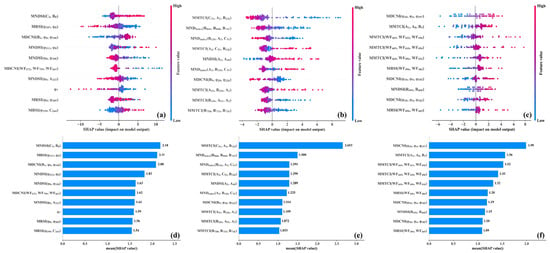
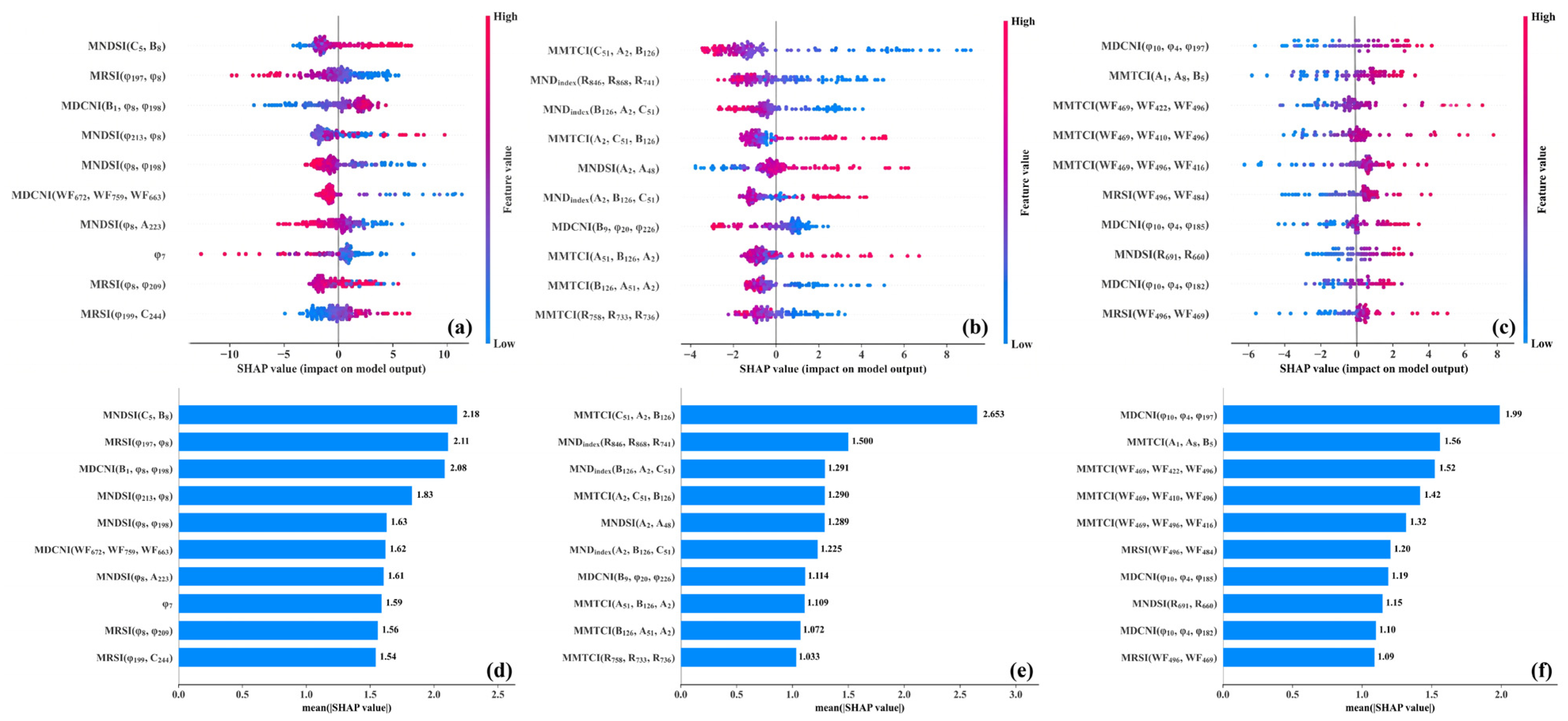
To quantify the relative contributions and the directions of the effects of input variables on LNA estimation, SHAP analysis was performed on the optimal model for each season (Figure 6). The results indicated that the top spectral features of LNA maintain a consistent positive effect across all seasons. In spring, MNDSI (e.g., MNDSI(C5, B8)) and MRSI rank highest, demonstrating distinct positive contributions. Summer LNA estimation relies primarily on MMTCI. Notably, MMTCI(C51, A2, B126) achieves the highest annual global importance (mean absolute SHAP = 2.653), and elevated values directly resulted in increased predictions. Finally, MDCNI (φ10, φ4, φ197) plays a dominant role in the autumn model, confirming its sustained positive impact on autumn LNA.
Figure 6.
Comprehensive feature importance analysis of LNA estimation models for spring, summer, and autumn. (a–c) SHAP beeswarm plots illustrating the distribution of the impacts of each feature on the model output; the color intensity reflects the feature value, with red indicating high values and blue indicating low values. (d–f) Feature importance ranking based on the mean absolute SHAP values for the respective seasons.
3.5. Assessment of Tea Plant N Status Using the LNA Monitoring Model at the Tea Plantation Scale
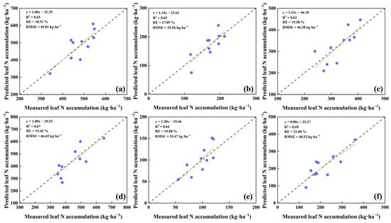
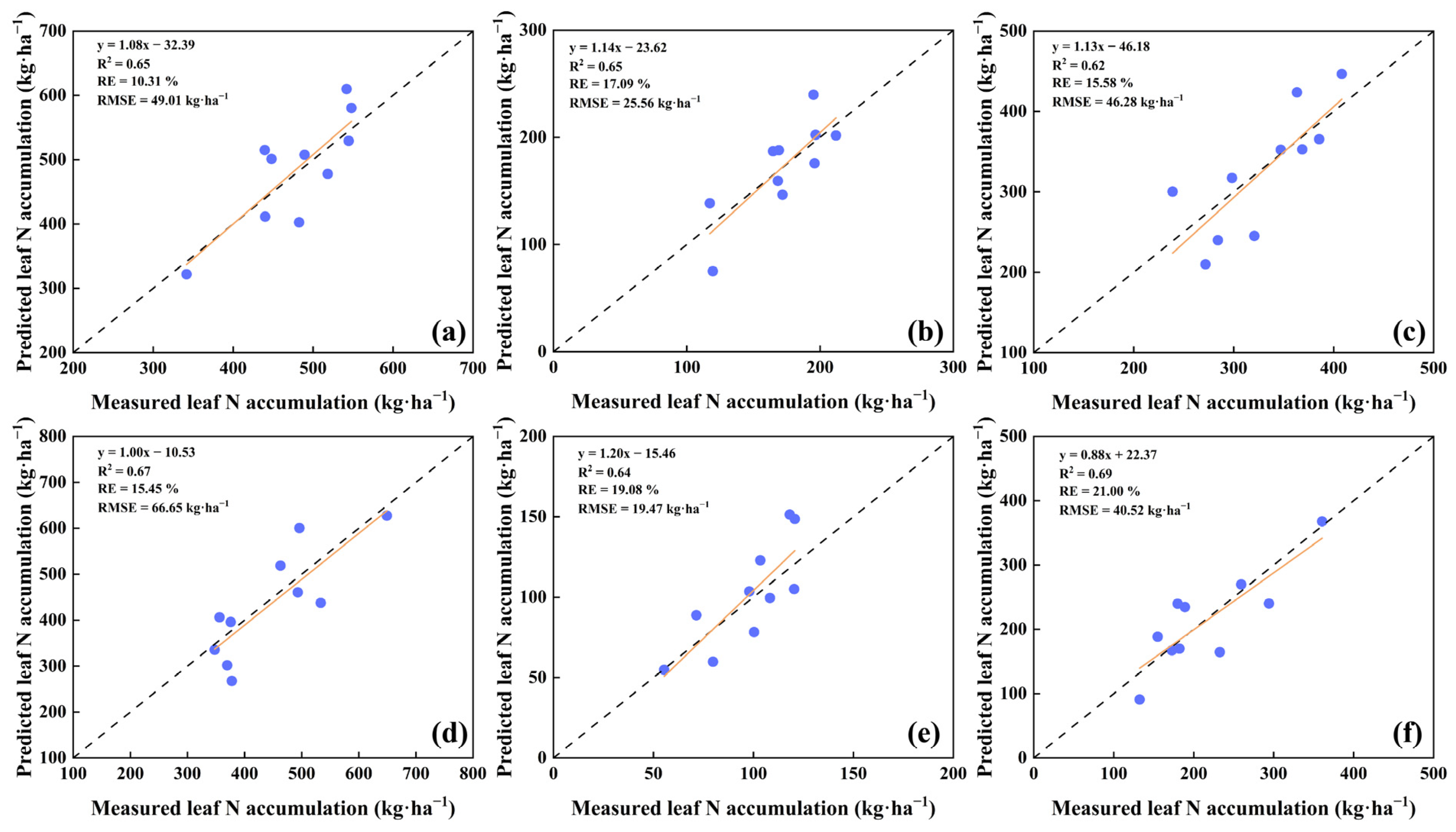
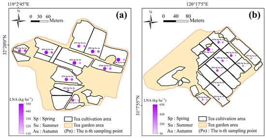
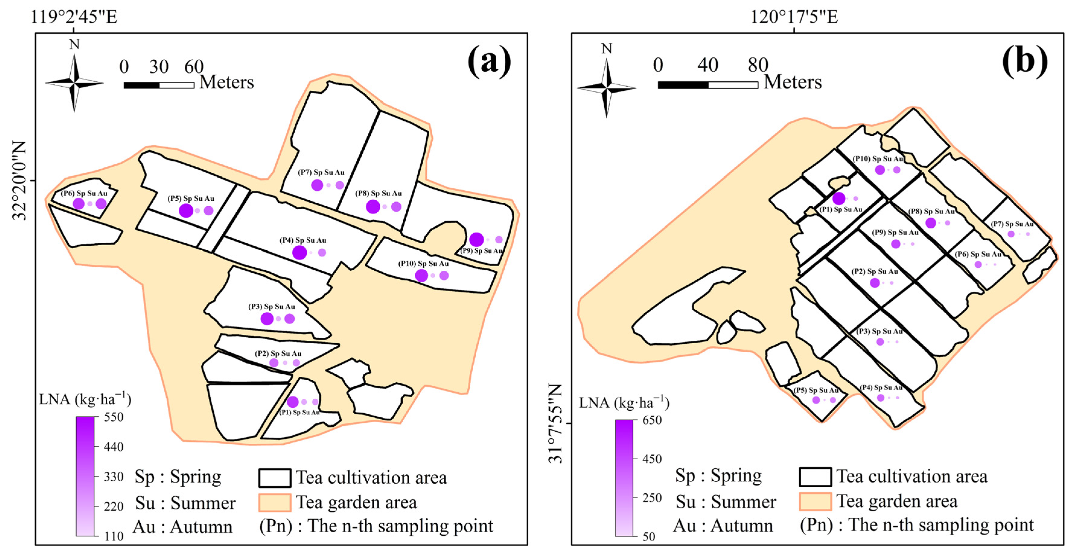
Using field-measured data from the Tianwangwu and Juyuanchun tea plantations, independent validation was conducted on the optimal predictive models selected for different seasons. Independent validation of each individual seasonal model demonstrated robust performance (Figure 7). Among these, the spring models achieved R2 values of 0.65 (RMSE = 49.01 kg·ha−1) for Juyuanchun and 0.67 (RMSE = 66.65 kg·ha−1) for Tianwangwu. The summer models yielded the lowest absolute errors, with RMSE dropping to 25.56 and 19.47 kg·ha−1, respectively. For the autumn models, Tianwangwu reached the highest R2 of 0.69, while Juyuanchun maintained a stable fit (R2 = 0.62, RMSE = 46.28 kg·ha−1). The linear regression equations between the measured and predicted LNA (Figure 7) showed slopes ranging from 0.88 to 1.20 across all independent validation sites. For the summer models, the slopes were 1.02 and 1.10. Furthermore, the relative errors ranged from 10.11% to 18.06% across different seasons. These metrics confirm the high reliability and transferability of these independent seasonal models for LNA estimation. Building upon this verified reliability, this study evaluated the spatiotemporal distribution of LNA across independently selected discrete test points in two tea plantations (Juyuanchun and Tianwangwu) using the developed LNA monitoring model. Figure 8 illustrates the spatial distribution and substantial statistical variability (as evaluated by CV) in LNA among these test points within each tea plantation. In Juyuanchun, LNA (closely associated with biomass) showed consistent seasonal dynamics, initially decreasing before increasing, with the highest annual levels in spring (LNA: 341.74–547.91 kg·ha−1). Spatial variability peaked in summer, with coefficients of variation of 17.65% for LNA. Similar seasonal trends were observed in Tianwangwu, where spring also exhibited the highest accumulation levels (LNA: 347.72–649.07 kg·ha−1), while spatial variability reached its maximum in autumn (CV = 31.07%). These results highlight the site-specific nature of tea plant N spatiotemporal dynamics and provide a theoretical foundation for zone-based management and precision nutrient regulation in tea cultivation.
Figure 7.
Independent validation results for predicting LNA in spring (a), summer (b), and autumn (c) in the Juyuanchun tea plantation; the independent validation results for predicting LNA in spring (d), summer (e), and autumn (f) in the Tianwangwu tea plantation.
Figure 8.
Maps of leaf N accumulation in Juyuanchun (a) and Tianwangwu (b) across spring, summer, and autumn.
4. Discussion
4.1. Mining Hyperspectral Features Sensitive to N Accumulation in Tea Plants
The high dimensionality of hyperspectral data provides rich biochemical information but also introduces redundant and physiologically irrelevant signals. Effective feature extraction is therefore essential for achieving accurate crop physiological assessments [21]. In this study, the continuous wavelet transform and harmonic decomposition were applied to extract spectral features prior to model construction. The results of feature extraction show that the most sensitive features for tea plant LNA varied across seasons, rather than being concentrated in a single stable spectral band. This pattern can be attributed to the fact that LNA combines leaf N concentration and biomass accumulation, with N affecting chlorophyll and photosynthetic protein pools, while biomass changes canopy scattering and leaf-layer structure, both of which exhibit seasonal variations [2]. In spring, the strongest R band was located at 595 nm, indicating sensitivity in the green-yellow region during rapid shoot expansion. In summer, sensitivity shifted to 721 nm in R, which is located in the red-edge domain where chlorophyll absorption transitions to NIR canopy scattering; red-edge indices have been shown to remain comparatively robust for canopy N monitoring across seasons [22]. In autumn, the sensitive spectral features moved to 403 nm, suggesting that short-wavelength visible information became more informative when mature tea canopies showed weaker red-edge dominance and stronger pigment-structure heterogeneity; recent hyperspectral work has reported an independent contribution of the blue spectral region to plant N assessment [23].
The continuous wavelet transform improved feature sensitivity because it retained local absorption and inflection geometry that R can dilute. The 566 nm, 739 nm, and 412 nm WF corresponded to the spring visible response, the summer red-edge response, and the autumn short-wave visible response, respectively, rather than arbitrary spectral positions. Preprocessing based on the continuous wavelet transform has been shown to strengthen N estimation by separating overlapping spectral information [7]. The results of this study further support this conclusion, because the strongest WF changed with season while remaining aligned with physiologically meaningful spectral regions. Harmonic decomposition separates R into phase components and amplitude components of different orders. The superiority of transformed features over R can be physiologically explained by the dual nature of LNA. Because LNA integrates leaf N concentration (a biochemical parameter) with canopy biomass (a structural parameter), mathematical transformations that can decouple these intertwined effects are highly advantageous. In this context, the continuous wavelet transform acts as an effective extractor of local biochemical absorption features, while harmonic decomposition serves as a robust descriptor of global canopy structural scattering. Harmonic decomposition separates R into phase components and amplitude components of different orders. Our results indicate that the phase component exhibits a higher sensitivity to tea plant LNA than to R and WF. For perennial tea plants, factors such as complex canopy structures and multiple leaf layers create pervasive background scattering that alters the entire canopy spectrum rather than just a narrow absorption band. Harmonic decomposition has recently been shown to extract structure-related N accumulation features by separating the dominant spectral energy from noise and structural interferences [9]. Of these, the phase component primarily captures the horizontal shift in the spectrum and is therefore highly sensitive to red-edge shifts induced by variations in chlorophyll degradation, N fluctuations, and canopy biomass [24]. Although HCs are not direct physical absorption features, they align closely with known physiological processes, indicating that different harmonic orders encode the biochemical and structural information embedded in hyperspectral data.
The constructed spectral indices further indicate that feature extraction improved not only feature sensitivity but also the physiological relevance of LNA-related spectral information. The stronger performance of optimized multi-feature indices is also consistent with Yang et al. [25], who showed that machine learning models fed with optimized spectral indices can improve crop N monitoring. The seasonal differences among the selected indices are agronomically meaningful rather than purely statistical. Spring-sensitive indices were mainly associated with rapidly expanding shoots and visible-region pigment responses, whereas summer indices emphasized red-edge and canopy vigor information. Red-edge indices have been reported to maintain relatively stable sensitivity to canopy N across seasons, which helps explain the summer shift toward red-edge-related index combinations [22]. In autumn, the superior performance of MDCNI(φ10, φ4, φ146) and MMTCI(WF469, WF422, WF496) suggests that harmonic- and wavelet-derived features captured accumulated canopy structure and heterogeneous leaf-layer effects more effectively than R. This interpretation is consistent with the nature of LNA as an integrated variable combining leaf N concentration and biomass accumulation, rather than a single biochemical trait [2]. Therefore, the season-specific indices identified in this study should be regarded as phenology-dependent spectral proxies, not interchangeable empirical formulas. Although the 400 to 890 nm spectral range employed in this study demonstrated robust capabilities in monitoring plant N by capturing pigment and structural responses as reliable biophysical proxies, exploring the shortwave infrared (SWIR) region presents a valuable opportunity for future refinement. The current visible and near-infrared (VNIR) domain effectively supports the high-accuracy estimations achieved in this research. However, incorporating the SWIR domain, which contains specific absorption overtones of N-bearing constituents such as proteins, would be highly beneficial for explicitly decoupling N signals from concurrent variations in leaf water and dry matter. Moving forward, integrating full-range hyperspectral data (350 to 2500 nm) with physically based radiative transfer models could further advance this methodology. Such an integration would facilitate the transition from empirical estimations to explicit biochemical retrievals, thereby continuously enhancing both the mechanistic interpretability and the overall robustness of the monitoring framework.
4.2. Machine-Learning-Based Modeling and Feature Interpretation for Monitoring LNA in Tea Plants
Differences in data sources and algorithmic structures can substantially influence model performance. Integrating multi-source sensitive features and spectral indices has therefore become an effective strategy to enhance predictive accuracy in crop biochemical monitoring [26]. In this study, the LNA monitoring model was evaluated using feature index datasets derived from individual data sources as well as HFI, in combination with three representative algorithms (RF, LASSO, and CNN). The results demonstrated that models constructed with HFI consistently outperformed those based on any single feature type. Compared with feature sets from individual sources, HFI integrates complementary hyperspectral information, thereby providing increased representational richness and enabling the LNA monitoring model to capture more complete spectral–physiological relationships. This finding aligns with previous work showing that combining multiple optimized spectral indices effectively reduces canopy structural interference and improves N monitoring accuracy (R2 = 0.82; [25]).
Among the traditional machine learning approaches, LASSO (R2 = 0.49–0.73) performed relatively well due to its L1 regularization mechanism, which mitigates multicollinearity while enabling sparse feature selection. However, its linear form limits its ability to represent some complex interactions among spectral indices [27]. RF demonstrated robustness to noise but exhibited distinct limitations in addressing the season-dependent nature of tea canopies. Because RF fundamentally relies on recursive orthogonal partitioning by splitting the data based on one individual feature index at a time, it struggles to systematically capture the deep, high-order synergistic interactions among the multi-domain features (i.e., RFI, WFFI, and HCFI). In perennial tea plants, where complex structural variations continuously confound biochemical N signals across seasons, the RF shallow learning mechanism often fails to fully decouple these interconnected physiological and structural dynamics. In contrast, the proposed CNN model overcomes these limitations through a deep, multi-source feature fusion architecture. Unlike existing crop monitoring models that directly feed R or single-domain empirical indices into shallow regressors, our strategy uniquely integrates multi-scale transformed features (WF and HC) with a tailored deep learning network. As designed in our methodology, the constructed multi-source feature index datasets (e.g., HFI) are flattened into one-dimensional sequences and processed through convolutional kernels of multiple sizes. This design allows the CNN to compute weighted combinations of multiple indices simultaneously, effectively forcing the deep integration of frequency-localized biochemical information (captured by WF) and canopy-structure-related periodic phase shifts (captured by HC). Through repeated convolution–pooling cycles, the model abstracts these cross-domain indices into high-order feature maps while actively filtering out redundant seasonal structural noise. This hierarchical feature fusion mechanism provides a clearer justification for adopting deep learning, as it effectively untangles the highly nonlinear relationships governing tea plant N accumulation better than conventional models across diverse seasonal stages [28,29,30]. Although the LNA monitoring model showed strong performance, further enhancements in spatiotemporal robustness are needed. Subsequent research will prioritize the assessment of model robustness under a wider array of growing conditions, tea cultivars, and management practices. Expanding training datasets with more representative canopy-level hyperspectral measurements will also help improve generalizability and support broader applications in precision tea cultivation.
Model interpretability is particularly important for hyperspectral N monitoring because high predictive accuracy alone does not demonstrate that a deep network has learned physiologically meaningful information. Recent agricultural XAI research has emphasized that black-box models may produce apparently strong predictions while potentially relying on unstable or context-specific correlations [13]. In spectral modeling, SHAP provides a practical way to decompose nonlinear model outputs into feature-level contributions, and recent studies have shown its value for explaining performance differences among full-spectrum, feature-spectrum, and attention-enhanced agricultural spectral models [14,15]. Therefore, the SHAP analysis in this study should be understood not only as a feature ranking procedure, but also as an interpretability check on whether the optimal LNA monitoring model relied on agronomically plausible spectral information. The SHAP results showed that the key variables driving LNA estimation maintained a consistently positive contribution across spring, summer, and autumn. In spring, MNDSI(C5, B8) and MRSI were dominant; in summer, MMTCI(C51, A2, B126) contributed most strongly; and in autumn, MDCNI(φ10, φ4, φ197) became the leading feature. These statistically dominant features correspond to spectral domains that previous empirical studies have closely linked to the biochemical modulation of chlorophyll and photosynthetic proteins by N enrichment [2,25]. This congruence indicates that the deep learning model relies on agronomically plausible spectral cues rather than spurious statistical artifacts. However, it should be noted that a positive SHAP value intrinsically quantifies a feature’s statistical contribution relative to a baseline prediction, rather than providing direct mechanistic evidence. Consequently, the SHAP interpretation primarily serves to validate the model’s decision-making logic from a statistical perspective. While these selected spectral features demonstrate high predictive value, inferring their explicit physiological roles or establishing causal relationships with N accumulation will require further empirical validation through direct biological diagnostics.
The seasonal shift in the highest-ranked SHAP features indicates that the model did not rely on a fixed spectral cue throughout the growth period, but rather changed its explanatory patterns in tandem with canopy development. During spring, model predictions were heavily driven by indices reflecting rapidly expanding leaves, whereas summer predictions shifted to rely predominantly on red-edge-related chlorophyll information. By autumn, harmonic phase features became increasingly important as they captured accumulated structural variations within the canopy over the growing season [31]. These temporal variations demonstrate that the HFI feature-fusion strategy effectively integrated complementary spectral information across distinct phenological stages, which explains its superior predictive performance to that of single-source feature sets [14]. However, because SHAP quantifies feature contributions based on statistical associations rather than causal relationships, feature importance may be redistributed among highly correlated hyperspectral variables. Consequently, the robustness and physiological relevance of these top-ranked features must be rigorously validated under controlled N fertilization gradients, across diverse tea cultivars, and in geographically independent plantations before they can be deployed as reliable diagnostic indicators for operational tea N management [32].
4.3. Application Prospects of the Tea Plant N Status Management Model Across Seasons
To achieve year-round monitoring of tea plant N status, this study evaluated the performance of the LNA monitoring model across spring, summer, and autumn. Owing to their perennial nature, tea plants experience distinct developmental phases and management regimes over the course of an annual growth period. Seasonal fluctuations in canopy characteristics (such as changes in leaf shape, tenderness, and greenness) can markedly influence R and consequently affect N estimation accuracy [33,34]. The LNA monitoring model demonstrated stable, reliable, moderate-to-good performance across all seasons (spring: R2 = 0.76; summer: R2 = 0.80; autumn: R2 = 0.70), indicating its considerable potential for continuous canopy monitoring and year-round field-level decision support. It is noteworthy that the predictive performance of the models exhibited seasonal variations (Figure 7), which are fundamentally driven by shifts in LNA distribution (Table 3) and physical canopy measurement conditions. The highest predictive stability was achieved in summer, facilitated by a relatively concentrated LNA distribution and a stable canopy structure that maximizes red-edge spectral efficacy. Conversely, the spring models faced the highest data variability (CV = 42.07%) driven by asynchronous shoot expansion, which introduces structural noise into spectral measurements and elevates prediction difficulty. In autumn, despite confronting the highest absolute LNA baseline (up to 397.63 kg·ha−1) due to biomass accumulation, the consistently low relative errors (RE < 16%) confirm that the models maintained robust proportional accuracy across extreme data spans.
Model application in the Juyuanchun and Tianwangwu plantations further revealed clear spatiotemporal heterogeneity in N accumulation. Juyuanchun showed the highest N levels in spring, while Tianwangwu exhibited pronounced spatial variability in autumn. These contrasting patterns highlight the need for a “one plantation, one strategy” nutrient management approach. Specifically, Juyuanchun would benefit from uniform spring fertilization to sustain its high biomass production, whereas Tianwangwu requires variable-rate fertilization in autumn (CV > 27%) to address substantial spatial heterogeneity. Unlike studies focusing on single time points [35], our multi-season mapping approach captures both temporal dynamics and spatial variation. This supports a fertilization strategy combining temporal targeting with spatial precision that mitigates nutrient waste and enhances resource use efficiency. The ability to dynamically map plantation-level N status also provides growers with timely and quantitative assessments of plant nutritional conditions, enabling more accurate evaluation of crop health, yield potential, and nutrient demand [36]. While validated using ground-based measurements, scaling this framework to Unmanned Aerial Vehicle (UAV) and satellite platforms is essential for large-scale operational monitoring. UAV hyperspectral imagery offers the opportunity to dynamically map continuous N status across entire plantations, advancing precision management. However, this transition introduces significant challenges, including mixed-pixel effects (e.g., soil and canopy shadows), Bidirectional Reflectance Distribution Function variations, and complex atmospheric attenuation. Furthermore, applying the WF and HC framework to multispectral satellites requires algorithmic adaptations due to their lower spectral resolutions. Consequently, future research will prioritize cross-platform calibration and validation.
5. Conclusions
This study demonstrated that WF and HC derived from the continuous wavelet transform and harmonic decomposition exhibit substantially higher sensitivity to tea plant N status than R. Based on these enhanced features, the two-feature and three-feature indices showed strong correlations with N parameters, demonstrating the effectiveness of data-driven hyperspectral index construction. The LNA estimation model developed with the CNN algorithm achieved consistently high predictive accuracy and showed moderate-to-good predictive performance across spring, summer, and autumn (R2 = 0.70–0.80), highlighting its strong temporal generalizability, supporting its potential for multi-season monitoring under the present conditions. SHAP analysis further indicated that the model relied on season-specific but physiologically plausible spectral cues, thereby strengthening the interpretability of the LNA monitoring model. Field validation in the Juyuanchun and Tianwangwu plantations revealed distinct plantation-specific spatiotemporal patterns in N accumulation, underscoring the value of the model in supporting customized nutrient management.
Supplementary Materials
The following supporting information can be downloaded at https://www.mdpi.com/article/10.3390/agriculture16212369/s1. Figure S1: Correlation coefficients between LNA and R (a), WF (b), and HC (c) in summer. Figure S2: Correlation coefficients between LNA and R (a), WF (b), and HC (c) in autumn. Figure S3: The two-feature spectral indices (MDSI, MNDSI and MRSI) derived from R (a–c), WF (d–f), and HC (g–i) were used to monitor LNA in summer. Note: The values in parentheses in each panel are the selected sensitive feature indices. Figure S4: The two-feature spectral indices (MDSI, MNDSI and MRSI) derived from R (a–c), WF (d–f), and HC (g–i) were used to monitor LNA in autumn. Note: The values in parentheses in each panel are the selected sensitive feature indices. Figure S5: The three-feature spectral indices (MDCNI, MMTCI and MNDindex) derived from R (a–c), WF (d–f), and HC (g–i) were used to monitor LNA in summer. Note: The values in parentheses in each panel are the selected sensitive feature indices. Figure S6: The three-feature spectral indices (MDCNI, MMTCI and MNDindex) derived from R (a–c), WF (d–f), and HC (g–i) were used to monitor LNA in autumn. Note: The values in parentheses in each panel are the selected sensitive feature indices.
Author Contributions
H.J. and J.J. contributed to conceptualization, methodology, investigation, validation, visualization, and writing—original draft. Y.L., S.Z., J.Y., H.G., Y.Y., X.Y., J.L., Q.S., Y.M., X.Z., W.F. and J.J. reviewed and edited the manuscript. Y.L., X.Y., J.L., Q.S., Y.M., X.Z., W.F. and J.J. were responsible for supervision. W.F. and J.J. were responsible for project administration and funding acquisition. All authors have read and agreed to the published version of the manuscript.
Funding
This research was funded by the China Agriculture Research System of MOF and MARA (CARS-18), Postdoctoral Fellowship Program of CPSF (GZC20240720), General Program of China Postdoctoral Science Foundation (2024M761440), Jiangsu Province Industry-University-Research Cooperation Project (BY20240370), Nanjing Digital Agriculture Science and Technology Achievement Integration Innovation and Demonstration Project (202510), Changzhou Agricultural Science and Technology Innovation Project (202506), Guizhou Provincial Science and Technology Plan Project (Qiankehe Foundation MS[2025]296), Qiannongkeyuan Outstanding Team ([2026]05), Guizhou Provincial Science and Technology Leading Talent Project (Qiankexie KJLYRC-[2026]033), Guizhou Provincial Key Core Technology Research for Mountain Agriculture (GZNYGJHX-2026011), Doctoral Fund Project of Guizhou Academy of Agricultural Sciences (202410) and Guizhou Province Tea Industry Technology System (GZCYCYJSTX-202606).
Data Availability Statement
The data that support the findings of this study are available from the authors upon reasonable request.
Conflicts of Interest
The authors declare no conflicts of interest.
Abbreviations
The following abbreviations are used in this manuscript:
| N | Nitrogen |
| R | Hyperspectral reflectance |
| LNA | Leaf nitrogen accumulation |
| WF | Wavelet features |
| HC | Harmonic components |
| CNN | Convolutional neural network |
| MDSI | Modified difference feature index |
| MNDSI | Modified normalized difference feature index |
| MRSI | Modified ratio feature index |
| MDCNI | Modified double-peak canopy N index |
| MMTCI | Modified MERIS terrestrial chlorophyll index |
| MNDindex | Modified red-edge normalized difference index |
| RF | Random forest |
| LASSO | Least absolute shrinkage and selection operator |
| RFI | Hyperspectral reflectance feature index dataset |
| WFFI | Wavelet features feature index dataset |
| HCFI | Harmonic components feature index dataset |
| HFI | The hybrid dataset combining RFI, WFFI, and HCFI |
| R2 | Coefficient of determination |
| RMSE | Root mean square error |
| RE | Relative error |
| SHAP | SHapley Additive exPlanations analysis |
References
- Mao, C.; He, J.; Wen, X.; Xiang, Y.; Feng, J.; Shu, Y. Correlation and pathway analysis of the carbon, nitrogen, and phosphorus in soil-microorganism-plant with main quality components of tea (Camellia sinensis). Phyton 2024, 93, 487–502. [Google Scholar] [CrossRef] [Scilit]
- Fu, Y.; Yang, G.; Pu, R.; Li, Z.; Li, H.; Xu, X.; Song, X.; Yang, X.; Zhao, C. An overview of crop nitrogen status assessment using hyperspectral remote sensing: Current status and perspectives. Eur. J. Agron. 2021, 124, 126241. [Google Scholar] [CrossRef] [Scilit]
- Corp, L.A.; Middleton, E.M.; Campbell, P.K.; Huemmrich, K.F.; Daughtry, C.S.; Russ, A.L.; Cheng, Y. Spectral indices to monitor nitrogen-driven carbon uptake in field corn. J. Appl. Remote Sens. 2010, 4, 043555. [Google Scholar] [CrossRef] [Scilit]
- Chen, P.; Haboudane, D.; Tremblay, N.; Wang, J.; Vigneault, P.; Li, B. New spectral indicator assessing the efficiency of crop nitrogen treatment in corn and wheat. Remote Sens. Environ. 2010, 114, 1987–1997. [Google Scholar] [CrossRef] [Scilit]
- Li, F.; Mistele, B.; Hu, Y.; Chen, X.; Schmidhalter, U. Comparing hyperspectral index optimization algorithms to estimate aerial N uptake using multi-temporal winter wheat datasets from contrasting climatic and geographic zones in China and Germany. Agric. For. Meteorol. 2013, 180, 44–57. [Google Scholar] [CrossRef] [Scilit]
- Yamashita, H.; Sonobe, R.; Hirono, Y.; Morita, A.; Ikka, T. Dissection of hyperspectral reflectance to estimate nitrogen and chlo-rophyll contents in tea leaves based on machine learning algorithms. Sci. Rep. 2020, 10, 17360. [Google Scholar] [CrossRef] [PubMed]
- Li, C.; Li, X.; Meng, X.; Xiao, Z.; Wu, X.; Wang, X.; Ren, L.; Li, Y.; Zhao, C.; Yang, C. Hyperspectral estimation of nitrogen content in wheat based on fractional difference and continuous wavelet transform. Agriculture 2023, 13, 1017. [Google Scholar] [CrossRef] [Scilit]
- Cheng, B.; Gao, Y. Hyperspectral anomaly detection via low-rank and sparse decomposition with cluster subspace accumulation. Sci. Rep. 2024, 14, 29530. [Google Scholar] [CrossRef] [Scilit] [PubMed]
- Liu, Y.; Feng, H.; Fan, Y.; Yue, J.; Chen, R.; Ma, Y.; Bian, M.; Yang, G. Improving potato above ground biomass estimation combining hyperspectral data and harmonic decomposition techniques. Comput. Electron. Agric. 2024, 218, 108699. [Google Scholar] [CrossRef] [Scilit]
- da Silva, B.C.; de Mello Prado, R.; Baio, F.H.R.; Campos, C.N.S.; Teodoro, L.P.R.; Teodoro, P.E.; Santana, D.C.; Fernandes, T.F.S.; da Silva Junior, C.A.; Loureiro, E.S. New approach for predicting nitrogen and pigments in maize from hyperspectral data and machine learning models. Remote Sens. Appl. Soc. Environ. 2024, 33, 101110. [Google Scholar] [CrossRef] [Scilit]
- He, J.; Song, Y.; Xie, D.; Liu, G. Integrating plant height into hyperspectral inversion models for estimating chlorophyll and total nitrogen in rice canopies. Agriculture 2026, 16, 656. [Google Scholar] [CrossRef] [Scilit]
- Yu, X.; Lu, H.; Liu, Q. Deep-learning-based regression model and hyperspectral imaging for rapid detection of nitrogen concentration in oilseed rape (Brassica napus L.) leaf. Chemom. Intell. Lab. Syst. 2018, 172, 188–193. [Google Scholar] [CrossRef] [Scilit]
- Hu, T.; Zhang, X.; Bohrer, G.; Liu, Y.; Zhou, Y.; Martin, J.; Li, Y.; Zhao, K. Crop yield prediction via explainable AI and interpretable machine learning: Dangers of black box models for evaluating climate change impacts on crop yield. Agric. For. Meteorol. 2023, 336, 109458. [Google Scholar] [CrossRef] [Scilit]
- Zhong, L.; Guo, X.; Ding, M.; Ye, Y.; Jiang, Y.; Zhu, Q.; Li, J. SHAP values accurately explain the difference in modeling accuracy of convolution neural network between soil full-spectrum and feature-spectrum. Comput. Electron. Agric. 2024, 217, 108627. [Google Scholar] [CrossRef] [Scilit]
- Wu, T.; Zhu, L.; Li, L.; Liu, L.; Bai, W.; Lin, L.; Yang, L. SHAPAttention: A novel approach to enhance model performance and interpretability in agricultural spectral data analysis. Comput. Electron. Agric. 2025, 236, 110445. [Google Scholar] [CrossRef] [Scilit]
- Tucker, C. Red and photographic infrared linear combinations for monitoring vegetation. Remote Sens. Environ. 1979, 8, 127–150. [Google Scholar] [CrossRef] [Scilit]
- Barnes, E.; Clarke, T.; Richards, S.; Colaizzi, P.; Haberland, J.; Kostrzewski, M.; Waller, P.; Choi, C.; Riley, E.; Thompson, T. Coincident detection of crop water stress, nitrogen status and canopy density using ground based multispectral data. In Proceedings of the Fifth International Conference on Precision Agriculture, Bloomington, MN, USA, 16–19 July 2000. [Google Scholar]
- Jordan, C. Derivation of leaf-area index from quality of light on the forest floor. Ecology 1969, 50, 663–666. [Google Scholar] [CrossRef] [Scilit]
- Dash, J.; Curran, P.J. The MERIS terrestrial chlorophyll index. Int. J. Remote Sens. 2004, 25, 5403–5413. [Google Scholar] [CrossRef] [Scilit]
- Sims, D.; Gamon, J. Relationships between leaf pigment content and spectral reflectance across a wide range of species, leaf structures and developmental stages. Remote Sens. Environ. 2002, 81, 337–354. [Google Scholar] [CrossRef] [Scilit]
- Moghimi, A.; Yang, C.; Marchetto, P.M. Ensemble feature selection for plant phenotyping: A journey from hyperspectral to multispectral imaging. IEEE Access 2018, 6, 56870–56884. [Google Scholar] [CrossRef] [Scilit]
- Patel, M.K.; Ryu, D.; Western, A.W.; Suter, H.; Young, I.M. Which multispectral indices robustly measure canopy nitrogen across seasons: Lessons from an irrigated pasture crop. Comput. Electron. Agric. 2021, 182, 106000. [Google Scholar] [CrossRef] [Scilit]
- Li, P.; Poblete, T.; Hornero, A.; Aryal, J.; Zarco-Tejada, P.J. Distinct contribution of the blue spectral region and far-red solar-induced fluorescence to needle nitrogen and phosphorus assessment in coniferous nutrient trials with hyperspectral imagery. Remote Sens. Environ. 2025, 328, 114915. [Google Scholar] [CrossRef] [Scilit]
- Shu, M.; Zhu, J.; Yang, X.; Gu, X.; Li, B.; Ma, Y. A spectral decomposition method for estimating the leaf nitrogen status of maize by UAV-based hyperspectral imaging. Comput. Electron. Agric. 2023, 212, 108100. [Google Scholar] [CrossRef] [Scilit]
- Yang, H.; Yin, H.; Li, F.; Hu, Y.; Yu, K. Machine learning models fed with optimized spectral indices to advance crop nitrogen monitoring. Field Crops Res. 2023, 293, 108844. [Google Scholar] [CrossRef] [Scilit]
- Ang, K.L.M.; Seng, J.K.P. Big data and machine learning with hyperspectral information in agriculture. IEEE Access 2021, 9, 36699–36718. [Google Scholar] [CrossRef] [Scilit]
- Tibshirani, R. Regression shrinkage and selection via the lasso. J. R. Stat. Soc. Ser. B 1996, 58, 267–288. [Google Scholar] [CrossRef] [Scilit]
- Hu, T.; Liu, Z.; Hu, R.; Tian, M.; Wang, Z.; Li, M.; Chen, G. Convolutional neural network-based estimation of nitrogen content in regenerating rice leaves. Agronomy 2024, 14, 1422. [Google Scholar] [CrossRef] [Scilit]
- Chen, B.; Li, Q.; Zhang, F.; Hu, Z. A multi-branch and multi-level feature extraction network model for near-infrared spectroscopy quantitative analysis. Infrared Phys. Technol. 2026, 153, 106264. [Google Scholar] [CrossRef] [Scilit]
- Pullanagari, R.; Dehghan-Shoar, M.; Yule, I.J.; Bhatia, N. Field spectroscopy of canopy nitrogen concentration in temperate grasslands using a convolutional neural network. Remote Sens. Environ. 2021, 257, 112353. [Google Scholar] [CrossRef] [Scilit]
- Jiang, J.; Ji, H.; Yan, Y.; Zhao, L.; Pan, R.; Liu, X.; Yin, J.; Duan, Y.; Ma, Y.; Zhu, X.; et al. Mining sensitive hyperspectral feature to non-destructively monitor biomass and nitrogen accumulation status of tea plant throughout the whole year. Comput. Electron. Agric. 2024, 225, 109358. [Google Scholar] [CrossRef] [Scilit]
- Lundberg, S.M.; Lee, S.-I. A Unified Approach to Interpreting Model Predictions. In Proceedings of the 31st International Conference on Neural Information Processing Systems, Long Beach, CA, USA; pp. 4768–4777.
- Batool, D.; Shahbaz, M.; Shahzad Asif, H.; Shaukat, K.; Alam, T.M.; Hameed, I.A.; Ramzan, Z.; Waheed, A.; Aljuaid, H.; Luo, S. A hybrid approach to tea crop yield prediction using simulation models and machine learning. Plants 2022, 11, 1925. [Google Scholar] [CrossRef] [Scilit] [PubMed]
- Meerdink, S.K.; Roberts, D.A.; King, J.Y.; Roth, K.L.; Dennison, P.E.; Amaral, C.H.; Hook, S.J. Linking seasonal foliar traits to VSWIR-TIR spectroscopy across California ecosystems. Remote Sens. Environ. 2016, 186, 322–338. [Google Scholar] [CrossRef] [Scilit]
- Jiang, J.; Ji, H.; Zhou, G.; Pan, R.; Zhao, L.; Duan, Z.; Liu, X.; Yin, J.; Duan, Y.; Ma, Y.C.; et al. Non-destructive monitoring of tea plant growth through UAV spectral imagery and meteorological data using machine learning and parameter optimization algorithms. Comput. Electron. Agric. 2025, 229, 109795. [Google Scholar] [CrossRef] [Scilit]
- Peng, J.; Ma, F.; Tian, D.; Quan, Q.; Chen, C.; Liao, J.; Zhou, Q.; Niu, S. Plant C:N ratio predicts community composition changes under N addition in an alpine meadow. J. Ecol. 2022, 111, 589–600. [Google Scholar] [CrossRef] [Scilit]

Disclaimer/Publisher’s Note: The statements, opinions and data contained in all publications are solely those of the individual author(s) and contributor(s) and not of MDPI and/or the editor(s). MDPI and/or the editor(s) disclaim responsibility for any injury to people or property resulting from any ideas, methods, instructions or products referred to in the content. |
© 2026 by the authors. Licensee MDPI, Basel, Switzerland. This article is an open access article distributed under the terms and conditions of the Creative Commons Attribution (CC BY) license.