


Abstract
Honeybees play vital roles in pollination, plant reproduction, agricultural productivity, and biodiversity. The Eastern honeybee, Apis cerana, is ecologically and economically important across South, Southeast, and East Asia. This study used an optimized Maximum Entropy (MaxEnt) model to assess current climatic suitability and potential future range dynamics of A. cerana across Asia, Europe, and Africa under SSP126, SSP245, and SSP585 scenarios for 2050 and 2070. The optimal model used the linear-quadratic-hinge (LQH) feature class with a regularization multiplier of 1 (RM = 1). Spatial cross-validation demonstrated strong and consistent performance, with mean AUC, TSS, and Continuous Boyce Index values of 0.852 ± 0.009, 0.617 ± 0.020, and 0.939 ± 0.013, respectively. Precipitation of the wettest month (Bio13) was the most influential predictor (~52%), followed by precipitation of the warmest quarter (Bio18) and mean diurnal range (Bio2). Current suitable habitats were concentrated mainly in South, Southeast, and East Asia. Future projections indicated a predominantly stable-to-expanding pattern of climatic suitability, with habitat gains generally increasing under stronger climate-forcing scenarios, particularly SSP585, while losses remained limited. Suitable habitats remained concentrated primarily across South and Southeast Asia, with additional suitable areas in parts of East Asia, Africa, and Australia. These projections represent potential climatic suitability rather than the realized distribution and provide a basis for monitoring potential expansions in climatically suitable habitat.
1. Introduction
Honeybees are essential components of terrestrial ecosystems, contributing substantially to pollination, plant reproduction, agricultural productivity, and the maintenance of global biodiversity [1,2]. Among the ecologically and economically important honeybee species in Asia, the Eastern honeybee, Apis cerana Fabricius 1793 (Hymenoptera: Apidae), is a widely distributed cavity-nesting species native to South, East, and Southeast Asia [3]. The species occurs across a broad range of climatic and environmental conditions, extending from tropical and subtropical regions to high-altitude mountainous landscapes, demonstrating remarkable ecological adaptability [3,4]. In particular, it has successfully established outside its native range in New Guinea, the Solomon Islands, and Australia due to its high adaptability [3]. Unlike the predominantly wild and open-nesting honeybees, which sympatrically inhabit many of the same regions, A. cerana frequently nests in enclosed cavities and human settlements, exhibiting a long history of traditional management and beekeeping throughout its native range [5,6].
The Eastern honeybee, A. cerana, serves as a critical pollinator of both wild flora and agricultural crops, supporting overall ecosystem functionality and food security [2,7]. Its capability to forage across diverse floral resources enables colonies to efficiently exploit seasonally available nectar and pollen, while specialized behavioral and physiological traits allow it to persist under variable environmental conditions [4]. Furthermore, A. cerana possesses distinct mechanisms contributing to ecological resilience, including defensive behaviors against predators, adaptation to local thermal extremes, and effective hygienic behaviors against parasites such as Varroa mites [3,8]. Consequently, A. cerana represents a key genetic resource for sustainable apiculture, particularly in regions where environmental stressors or climate extremes challenge introduced species like Apis mellifera [6].
Beyond its ecological role, A. cerana holds substantial socioeconomic value. It is widely managed by rural and small-scale beekeepers for honey, beeswax, and royal jelly, providing supplementary income and stabilizing local livelihoods [3,9]. Because the species is naturally adapted to regional Asian environments, A. cerana is particularly suited for low-input, locally adapted beekeeping systems [6]. Its pollination activity further enhances crop productivity, significantly increasing yields in fruits, vegetables, oilseeds, and other flowering agricultural crops [7].
Despite its ecological and economic importance, populations of A. cerana are increasingly threatened by environmental and anthropogenic pressures. Habitat loss, land conversion, agricultural intensification, pesticide exposure, climate change, and competition with introduced species jeopardize colony survival and long-term persistence [4,10,11]. In particular, climate change is increasingly influencing species distributions and modifying the ecological niches of key pollinators [12,13]. Additionally, shifts in temperature and precipitation regimes can alter floral phenology, reduce resource availability, and disrupt foraging activity [14,15]. Understanding the geographic distribution and environmental niche of A. cerana is therefore crucial for identifying suitable habitats, forecasting range shifts under climate change scenarios, and informing effective conservation management [4,16].
Species Distribution Models (SDMs) provide a robust framework for analyzing relationships between species occurrence records and environmental variables to predict potential habitat suitability [17,18,19]. SDMs have been successfully used to model the distributions of different honeybee species [20,21,22]. For A. cerana, SDM approaches can identify environmentally suitable areas, characterize spatial shifts and changes in habitat connectivity under environmental change, and provide baseline information to support conservation planning and apicultural management strategies [4]. Consequently, this study aims to evaluate potential spatial shifts and climatic suitability expansion in the distribution of A. cerana across regions of Asia, Europe, and Africa where potential terrestrial routes for expansion exist. A key novelty of this study lies in addressing the limited knowledge regarding optimal habitat suitability for A. cerana and its potential range shifts under projected climate scenarios for 2050 and 2070. In doing so, this research fills a critical geographic knowledge gap while providing broader insights into the long-term impacts of climate change on this ecologically and economically important pollinator.
2. Materials and Methods
2.1. Occurrence Data Filtering and Spatial Thinning
Occurrence records for A. cerana were retrieved from the Global Biodiversity Information Facility (GBIF) on August 2026 (https://doi.org/10.15468/dL.jj6gts, accessed on 16 August 2026). The download comprised 15,620 occurrence records obtained using the following filters: occurrence status restricted to “present,” scientific name restricted to A. cerana, basis of record restricted to human observations, and observation years limited to 2020–2026. This temporal restriction was applied to provide a contemporary representation of the species’ distribution, considering that A. cerana is managed in many regions and its distribution may be influenced by human-mediated activities. The use of recent records was intended to better reflect its current distribution and reduce potential discrepancies associated with older observations. The downloaded dataset included records from 22 datasets. Taxonomic information in the download was populated using the Catalogue of Life. To ensure data quality and geographic reliability, the occurrence records were cleaned using R (version 4.5.1). The original dataset contained 15,620 records. Column names and coordinate fields were standardized to ensure consistency. Coordinates were converted to numeric values, and records with missing latitude or longitude were removed, excluding 30 records and retaining 15,590 occurrences (99.81%). Exact duplicates, defined as records with identical longitude and latitude, were then removed, leaving 13,844 records (88.63%).
Coordinate quality was assessed using CoordinateCleaner, including checks for invalid and zero coordinates, equal latitude and longitude values, and marine locations. All 13,844 records passed these tests. The records were converted to spatial objects using WGS84 (EPSG:4326) and restricted to the modelling extent of 20° W–180° E longitude and 60° S–60° N latitude, with no additional records removed. Marine records were subsequently removed by intersecting occurrences with Natural Earth global land polygons. This excluded 1600 records, leaving 12,244 terrestrial occurrences (78.39%). Records occurring within Europe were then excluded using Natural Earth country boundaries, removing an additional six records and leaving 12,238 occurrences (78.35%).
To reduce spatial autocorrelation and uneven sampling intensity, spatial thinning was performed using spThin with a minimum distance of 50 km, one replicate, and a fixed random seed (123). This resulted in 870 final occurrence records (5.57% of the original dataset), which were used in subsequent analyses (Supplementary Materials File S1).
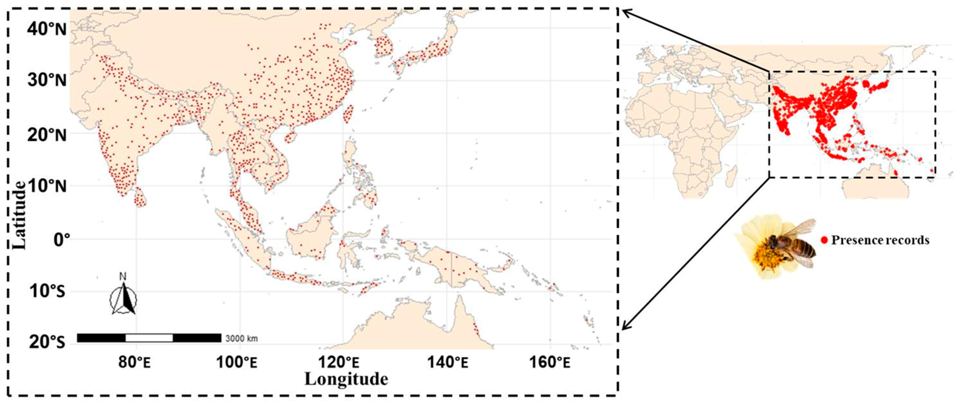
The cleaned and thinned occurrences were mapped using Natural Earth country boundaries within the defined study extent. An additional high-resolution map was produced using a buffered bounding box based on the geographic range of the final records (Figure 1).
Figure 1.
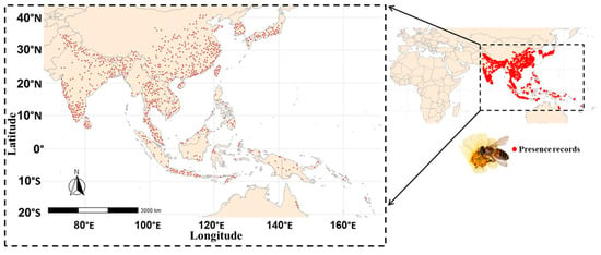
Spatial distribution of the 870 occurrence records of Apis cerana included in this study across its geographic range.
2.2. Environmental Data and Predictor Selection
All data processing, environmental data preparation, species distribution modeling, model evaluation, and visualization were conducted in R (version 4.5.1). Occurrence records obtained after the geographic cleaning and spatial-thinning procedure described above were used as the input dataset for ecological niche modeling. Environmental predictors were obtained from the WorldClim version 2.1 [23,24,25,26] bioclimatic dataset at a spatial resolution of 10 arc-minutes. All 19 standard bioclimatic variables (BioClim 1–19) were loaded as raster layers and cropped to the modelling extent of 20° W–180° E longitude and 60° S–60° N latitude.
The species’ accessible area (M region) was primarily defined using the boundaries of Asian countries obtained from Natural Earth. To ensure that occurrence records located outside these country boundaries were also encompassed within the accessible area, a 600-km buffer was applied around the occurrence localities (Supplementary Figure S1; File S2). Thus, the M region represents the Asian country boundaries expanded by a 600-km buffer around the available occurrence records, providing a spatially constrained calibration area for model development. To avoid geographic distortion during buffering, occurrence points and country polygons were projected to the World Cylindrical Equal Area projection. The buffered occurrences were then combined with the Asian polygons, transformed back to WGS84, validated, and intersected with Natural Earth global land polygons to retain terrestrial areas only. The resulting M region was used to crop and mask the bioclimatic rasters. Its spatial alignment with the occurrence records was visually inspected within the predefined modelling extent.
Environmental values for all 19 bioclimatic variables were extracted at the occurrence locations within the accessible area. Pearson correlations among the climatic variables were calculated and visualized as a heatmap to assess potential multicollinearity (Supplementary Figure S2; File S2).
Environmental predictors were filtered using the vifcor function with a correlation threshold of |r| = 0.7. This procedure reduced the 19 variables to seven predictors: Bio2, Bio3, Bio8, Bio13, Bio14, Bio18, and Bio19, representing mean diurnal range, isothermality, mean temperature of the wettest quarter, precipitation of the wettest month, precipitation of the driest month, precipitation of the warmest quarter, and precipitation of the coldest quarter, respectively.
A second Pearson correlation matrix was calculated for the seven selected variables to confirm that predictor redundancy had been substantially reduced (Supplementary Figure S3; File S2). The seven selected variables were retained in both the M-region raster stack and the full modelling-extent raster stack. The M-region layers were used for model calibration and background sampling, while the full-extent layers supported subsequent geographic projections.
2.3. Environmental Background Sampling and Spatial Block Cross-Validation
To characterize environmental conditions within the accessible area (M), 10,000 background points were randomly sampled from the selected environmental predictors, excluding cells with missing values. Geographic coordinates and corresponding environmental values were retained for subsequent modelling. A fixed random seed of 42 was used to ensure reproducibility.
To account for spatial autocorrelation and provide a more realistic model evaluation, spatially structured cross-validation was implemented. Environmental rasters, occurrence records, and background points were projected to Web Mercator so that distances and block dimensions could be defined in metres.
Spatial blocks were generated using cv_spatial with five-fold cross-validation and a 600-km block size. Fold allocation was optimized through random selection over 100 iterations. The resulting spatial partition divided occurrences into five geographically independent training and testing subsets. Testing folds contained 162–189 occurrence records, while training sets contained approximately 681–708 records per fold.
Occurrence fold assignments were retained for model calibration and evaluation. Background points were assigned to the same folds according to the spatial block in which they occurred. Thus, occurrence and background data followed the same spatial cross-validation structure.
This spatial blocking reduced the potential for overly optimistic model performance caused by spatially clustered training and testing records, providing a more robust assessment of predictive performance and geographic transferability.
2.4. Model Tuning and Selection
Model complexity and regularization were optimized using the ENMeval framework within the previously defined accessible area (M). Models were fitted using maxnet with the cleaned occurrence records and 10,000 background points. The previously generated five-fold spatial cross-validation partitions were supplied as user-defined groups for both occurrence and background data to account for spatial autocorrelation during model tuning. Three feature-class (FC) combinations—L, LQ, and LQH—and four regularization multipliers (RM: 0.5, 1, 2, and 3) were evaluated, resulting in 12 candidate models. Models were assessed using the mean validation Area Under the Curve (AUC) and the corrected Akaike Information Criterion (AICc). Models were ranked primarily using ΔAICc, with the lowest value indicating the preferred configuration. The optimal model used the LQH feature classes with RM = 1.0, achieving a mean validation AUC = 0.852 (Supplementary Table S1; File S3). Its substantially lower ΔAICc indicated a favourable balance between model fit and complexity.
2.5. Model Evaluation
The predictive performance of the selected model was evaluated using the same five-fold spatial cross-validation scheme. For each fold, the model was calibrated using occurrence and background records from four training folds and independently evaluated on the remaining testing fold. Models were fitted using the optimal LQH feature classes and regularization multiplier = 1, with predictions generated using the cloglog output transformation. Performance was assessed using AUC, True Skill Statistic (TSS), Continuous Boyce Index (CBI), specificity, sensitivity, and omission rate. AUC measured discrimination between occurrence and background locations, while TSS provided a threshold-dependent measure of discrimination. CBI assessed agreement between predicted suitability and observed occurrences. Sensitivity and specificity were calculated using the optimal classification threshold, and omission rate represented the proportion of testing occurrences predicted below this threshold.
For consistent comparison among spatial folds, sensitivity was interpolated across a common range of specificity values. All evaluation metrics were calculated separately for each of the five folds and summarized using their mean and standard error, providing an overall assessment of model predictive performance and spatial transferability.
Response curves were generated for each cross-validation model to examine the relationship between individual environmental predictors and predicted habitat suitability. For each predictor, values were varied across their observed environmental range while the remaining predictors were held at their mean values. Suitability was predicted using the cloglog transformation, allowing the response patterns of the seven selected bioclimatic variables to be compared across the five cross-validation models.
Variable importance was assessed using a permutation-based approach. The fitted optimal MaxEnt model was first used to calculate the baseline AUC, after which the values of each environmental variable were randomly permuted while all other variables remained unchanged. The model was then re-evaluated using the permuted data, and variable importance was calculated as the decrease in AUC relative to the baseline. Negative AUC changes were set to zero, and the resulting importance values were standardized to percentages by dividing each variable’s AUC decrease by the sum of all AUC decreases and multiplying by 100.
A jackknife analysis was conducted to assess the relative importance and unique contribution of the seven selected bioclimatic variables to the optimized maximum entropy model. Records with missing environmental values or presence–background classifications were excluded before analysis. The baseline AUC of the full model, using the cloglog transformation, was calculated as the reference for evaluating individual predictor contributions. For each environmental variable, two models were fitted using the optimal LQH feature classes and regularization multiplier = 1.0. First, a model using only the focal variable was fitted to assess its independent predictive information. Second, a model containing all selected variables except the focal variable was fitted. Variable importance was quantified as the decrease in AUC after removing the variable: AUC decrease = AUC of full model − AUC of model without the variable.
A larger AUC decrease indicated a greater contribution to overall model performance, whereas a smaller decrease indicated limited additional information beyond the other predictors. The analysis was repeated for Bio2, Bio3, Bio8, Bio13, Bio14, Bio18, and Bio19. Results included the AUC of models using each variable alone and the AUC of models excluding each variable. A jackknife bar plot was used to rank predictors according to their AUC decrease, providing a direct comparison of their relative importance in the optimized species distribution model.
Following model tuning and evaluation, the final maximum entropy model was fitted using all cleaned occurrence records and the complete set of background points sampled within the accessible area (M). The model used the seven selected bioclimatic predictors, the optimal LQH feature-class combination, and a regularization multiplier of 1.0. This optimized model was subsequently used to predict environmental suitability across the broader geographic modelling extent.
2.6. Current Habitat Suitability
The final optimized maximum entropy model was projected across the full modelling extent (20° W–180° E and 60° S–60° N) using the seven selected bioclimatic predictors. Predictions were generated using the cloglog transformation, producing continuous suitability values from 0 to 1. The resulting raster represented relative environmental suitability across the study area.
Two continuous suitability maps were produced: one showing the predicted suitability surface alone and another with the cleaned occurrence records overlaid to compare observed locations with areas of predicted high suitability.
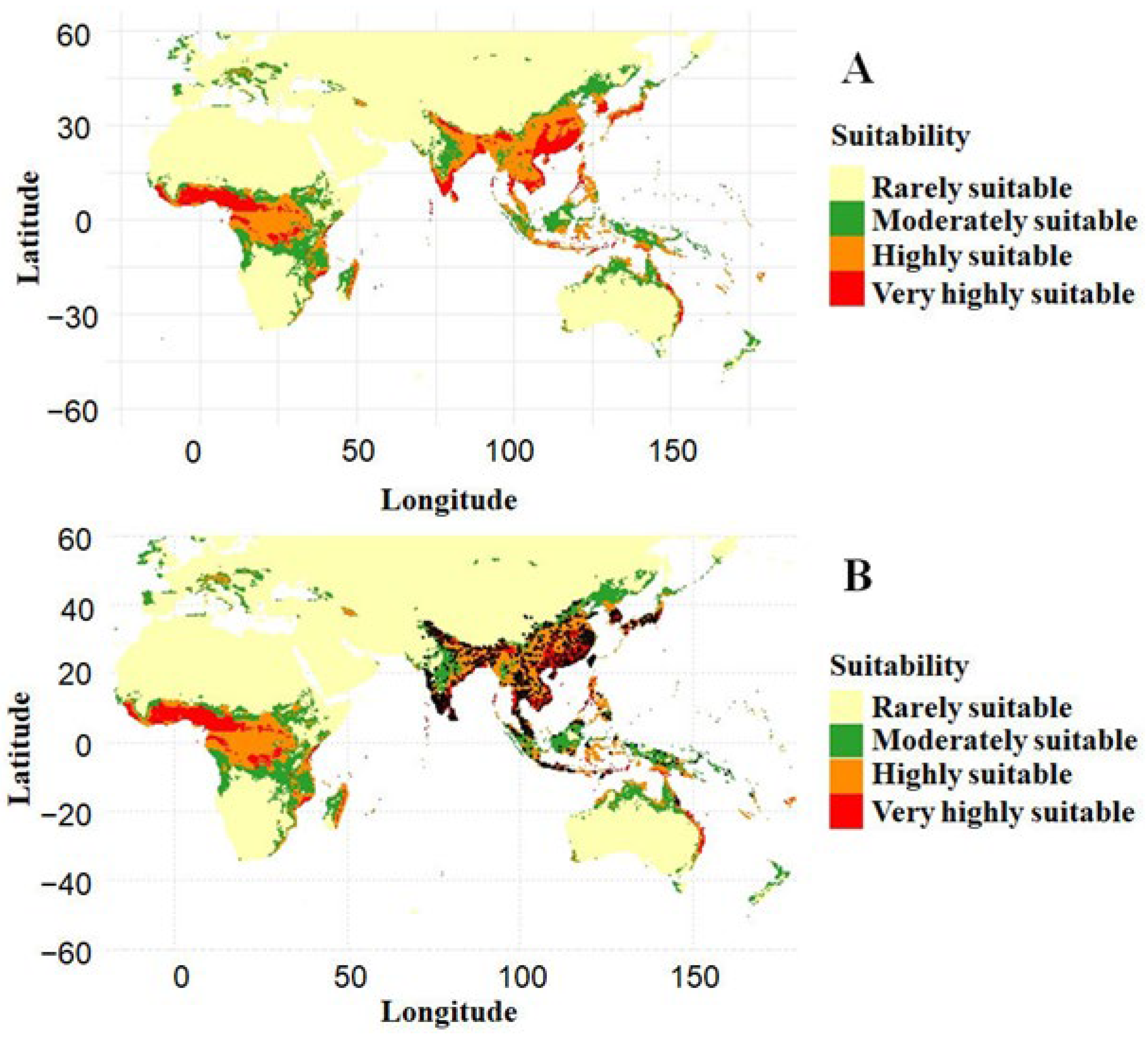
For spatial interpretation, continuous predictions were classified into four categories: 0.00–0.25 = rarely suitable, >0.25–0.50 = moderately suitable, >0.50–0.75 = highly suitable, and >0.75–1.00 = very highly suitable [27]. The geographic area of each category was calculated and expressed as a percentage of the total analysed area.
Finally, the classified raster was converted to a spatial data frame, and two categorized suitability maps were generated: one displaying the four suitability classes alone and another with occurrence records overlaid. These maps were used to visualize the spatial distribution of predicted suitability and its correspondence with observed occurrences.
2.7. Future Climate Scenarios
Future habitat suitability was projected for 2050 and 2070 using the optimized current-climate MaxEnt model (optimal_maxnet) and the same seven selected bioclimatic variables, ensuring that differences between current and future predictions reflected climatic changes rather than changes in model structure or predictors.
Projections covered 20° W–180° E longitude and 60° S–60° N latitude, encompassing Africa, Europe, and Asia. Future climate data were processed separately for each period, with the required BioClim layers automatically matched to the predictors used during model calibration. Habitat suitability was predicted using maxnet and the cloglog transformation, producing continuous values from 0 to 1.
Climate uncertainty was represented using three GCMs (IPSL-CM6A-LR, BCC-CSM2-MR, and MPI-ESM1-2-HR) under three SSPs (SSP126, SSP245, and SSP585). Thus, nine GCM–SSP projections were generated for each future period. For each SSP, predictions from the three GCMs were averaged to produce three SSP-specific ensemble maps. A grand ensemble was also generated by averaging all nine GCM–SSP projections, integrating uncertainty from both climate models and emission scenarios.
Continuous suitability predictions were visualized and classified into four categories, as described in the previous section. Maps were produced for individual GCM–SSP projections, SSP ensembles, and the grand ensemble for both 2050 and 2070.
The area occupied by each suitability class was calculated using raster cell areas from the cellSize function in terra, which accounts for geographic variation in cell size. Areas were summed for each class and expressed as a percentage of the total modelled area for every projection and ensemble.
2.8. Changes in Habitat Distribution
Spatial range shifts were assessed across the modelling extent (20° W–180° E, 60° S–60° N) using the optimized model and the selected bioclimatic predictors. Habitat suitability was projected for 2050 and 2070 using three GCMs (IPSL-CM6A-LR, BCC-CSM2-MR, and MPI-ESM1-2-HR) under three SSPs (SSP126, SSP245, and SSP585), resulting in nine GCM–SSP projections per period. Future BioClim predictors were matched to the model variables and cropped to the common extent. Continuous suitability (0–1) was predicted using the cloglog transformation. For each SSP, the three GCM predictions were averaged cell-by-cell to generate SSP-specific ensembles, and a grand ensemble was calculated from all nine projections.
Current, 2050, and 2070 suitability maps were converted to binary suitable/unsuitable maps using the mean five-fold spatial block cross-validation threshold of 0.385 (≥0.385 = suitable). The same threshold was applied across all periods to ensure comparability. Raster map algebra was used to classify changes into four categories: unsuitable (unsuitable in both periods), loss (suitable initially but unsuitable subsequently), gain (unsuitable initially but suitable subsequently), and stable (suitable in both periods).
Range shifts were evaluated for the current–2050, current–2070, and 2050–2070 periods across individual GCM–SSP projections, SSP ensembles, and the grand ensemble. The area of each category was calculated using terra::cellSize and expressed as a percentage of the total valid area. Range-shift maps were generated using ggplot2 with a consistent geographic extent and coordinate system to visualize habitat loss, gain, and persistence across climatic periods.
2.9. Multivariate Environmental Similarity Surface (MESS) Analysis
MESS analysis was performed using the terra and predicts packages to assess environmental similarity between future climatic conditions and those represented by current A. cerana occurrence records. Reference environmental values were extracted from the selected baseline environmental layers at occurrence locations. MESS surfaces were generated for 2050 and 2070 across three CMIP6 GCMs (IPSL-CM6A-LR, BCC-CSM2-MR, and MPI-ESM1-2-HR) and three SSPs (SSP126, SSP245, and SSP585), using the selected model predictors within the study area. For each SSP, the three GCM-specific MESS surfaces were averaged to generate an SSP ensemble, while an overall ensemble was calculated by averaging all nine GCM–SSP MESS surfaces. Novel-climate areas were quantified using binary MESS masks, with cell areas calculated using terra::cellSize, and expressed as a percentage of the total study area.
3. Results
3.1. Model Performance
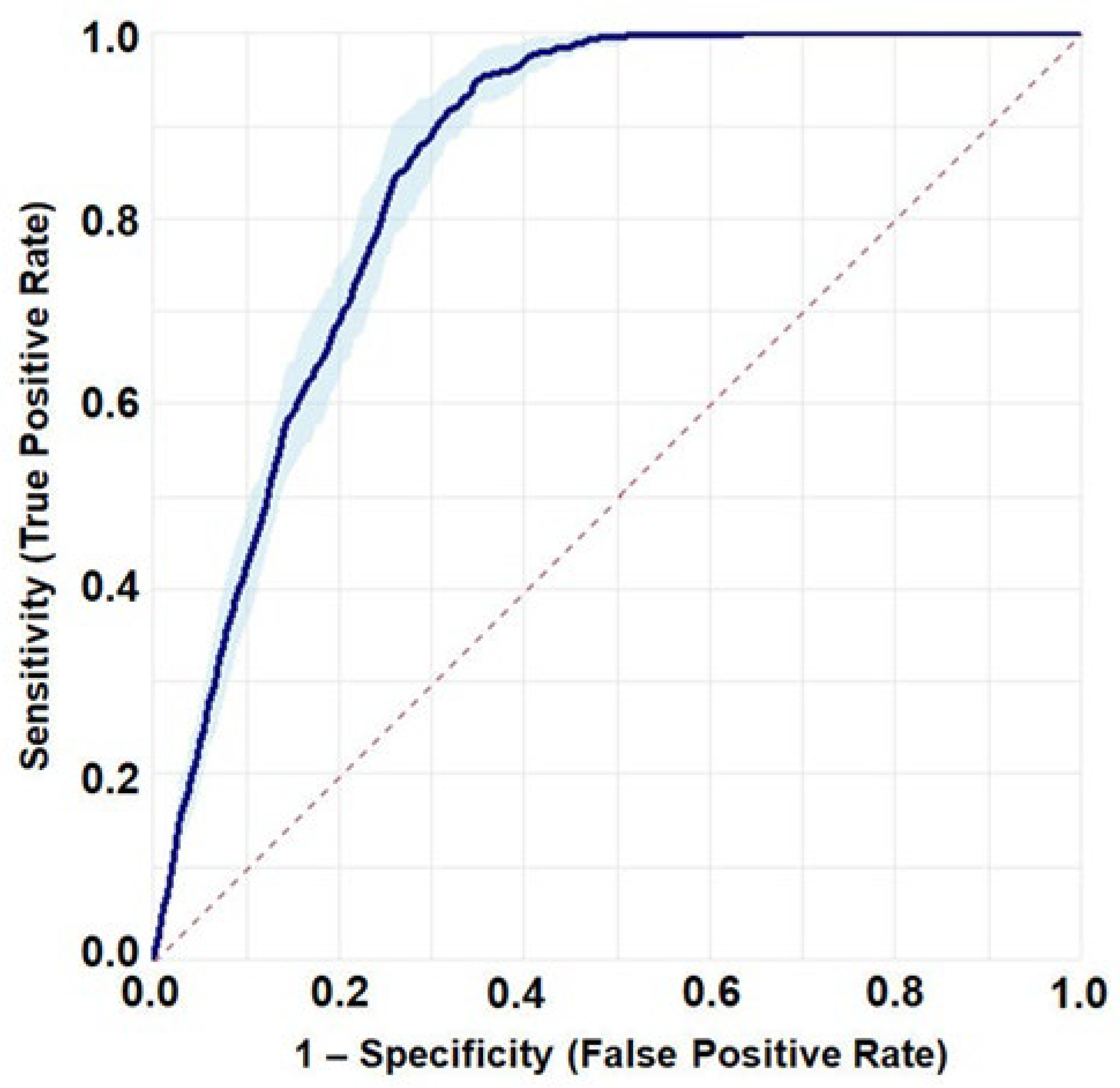
The optimized MaxEnt model (LQH, RM = 1) demonstrated strong predictive performance and consistency across the five spatial cross-validation folds. The mean AUC across the final five-fold spatial cross-validation was 0.852 ± 0.009 (Figure 2), indicating good discrimination between presence and background locations. The model also achieved a mean TSS of 0.617 ± 0.020, indicating good discriminatory performance across the spatial validation folds. The mean CBI was 0.939 ± 0.013, providing further evidence of strong model predictive performance and its ability to identify suitable habitats. At the mean optimal threshold of 0.385 ± 0.028, the model achieved a high mean sensitivity of 0.928 ± 0.013 and a specificity of 0.690 ± 0.018. The corresponding mean omission rate was 0.072 ± 0.013, indicating a relatively low proportion of observed presence locations incorrectly classified as unsuitable across the spatial validation folds. These results demonstrate that the optimized MaxEnt model provided reliable predictions of habitat suitability under spatially structured five-fold cross-validation.
Figure 2.
Receiver operating characteristic (ROC) curve illustrating the predictive performance of the optimized MaxEnt model under five-fold spatial cross-validation. The solid line represents the mean ROC curve across validation folds, the shaded area denotes the corresponding 95% confidence interval, and the dashed diagonal line indicates the performance expected under random discrimination.
3.2. Climatic Response Patterns
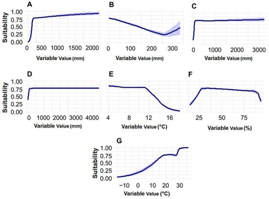
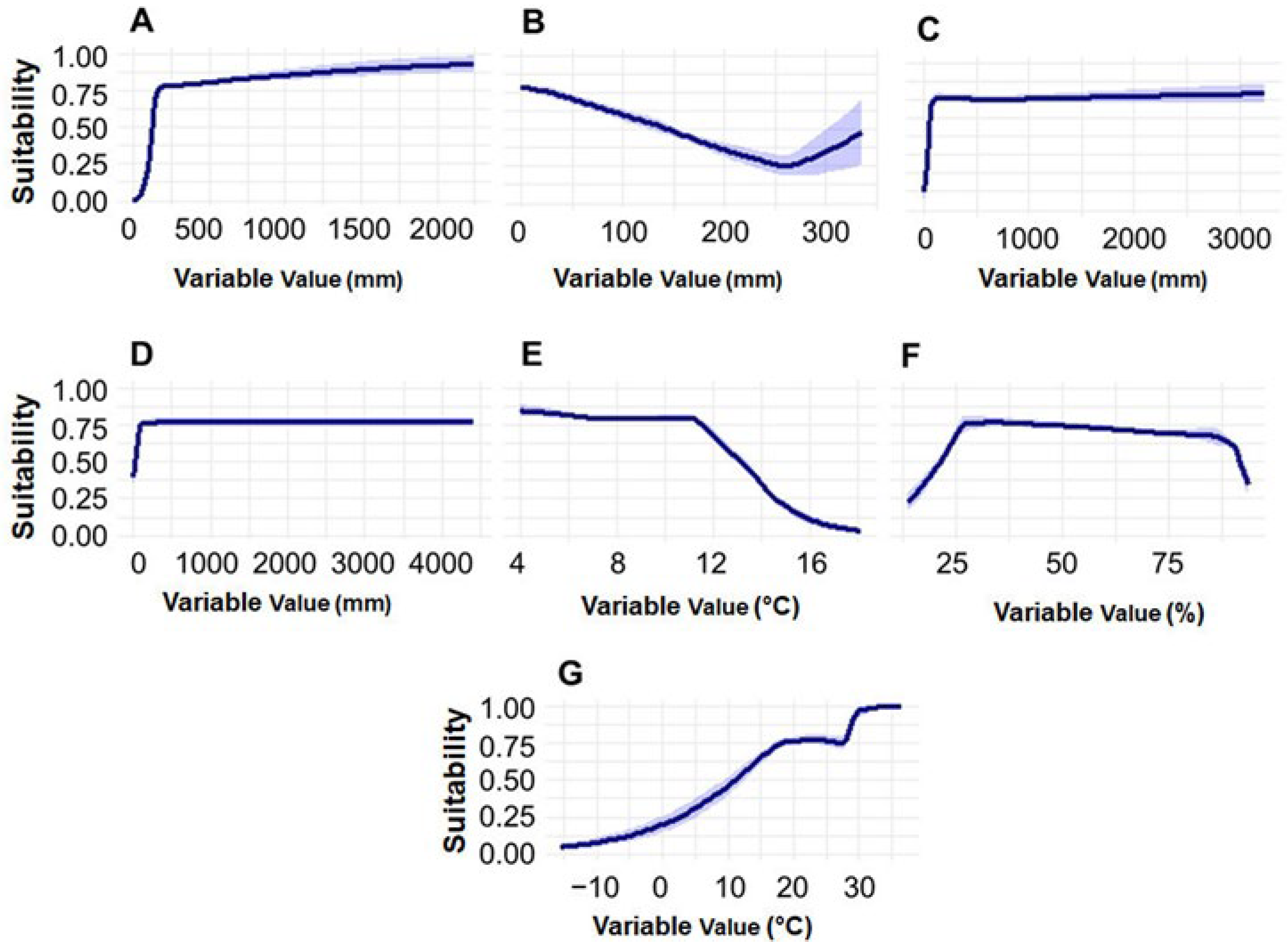
The response curves describing the relationship between the predicted habitat suitability for A. cerana and the selected bioclimatic variables are shown in Figure 3. Suitability increased sharply with increasing precipitation during the wettest month (Bio13), reaching a high plateau at approximately 200–300 mm and remaining consistently high at greater precipitation levels. A similar pattern was observed for precipitation during the warmest quarter (Bio18) and precipitation during the coldest quarter (Bio19), where habitat suitability increased rapidly at relatively low precipitation levels and subsequently remained high and stable. In contrast, the response to precipitation during the driest month (Bio14) showed a negative relationship across most of the observed range, with suitability declining as precipitation increased up to approximately 250 mm, followed by a slight increase at higher values.
Figure 3.
Response curves showing the relationship between predicted habitat suitability for Apis cerana and selected bioclimatic variables. Solid lines represent the mean response across cross-validation folds, while shaded bands indicate ±1 standard deviation among folds. (A) Precipitation of wettest month (Bio13); (B) Precipitation of driest month (Bio14); (C) Precipitation of warmest quarter (Bio18); (D) Precipitation of coldest quarter (Bio19); (E) Mean diurnal range (Bio2); (F) Isothermality (Bio3; BIO2/BIO7 × 100); and (G) Mean temperature of wettest quarter (Bio8).
Mean diurnal temperature range (Bio2) also exhibited a negative response, with high suitability at lower values (approximately 4–10 °C) and a marked decline as the diurnal range increased beyond approximately 11–12 °C. The response to isothermality (Bio3) indicated that suitability increased rapidly at lower values, reached an optimum at intermediate values (approximately 25–35), and gradually declined at higher values, with a pronounced decrease at the upper extreme. For mean temperature of the wettest quarter (Bio8), suitability generally increased with temperature, rising substantially from approximately 0 °C and reaching high suitability at around 20 °C, followed by a further increase at temperatures above approximately 30 °C.
The relatively narrow shaded bands across most response curves indicate consistent predictions among the cross-validation folds, although greater variability was observed at the extreme upper range of Bio14.
3.3. Importance of the Selected Environmental Predictors
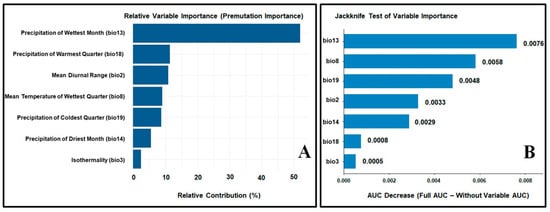
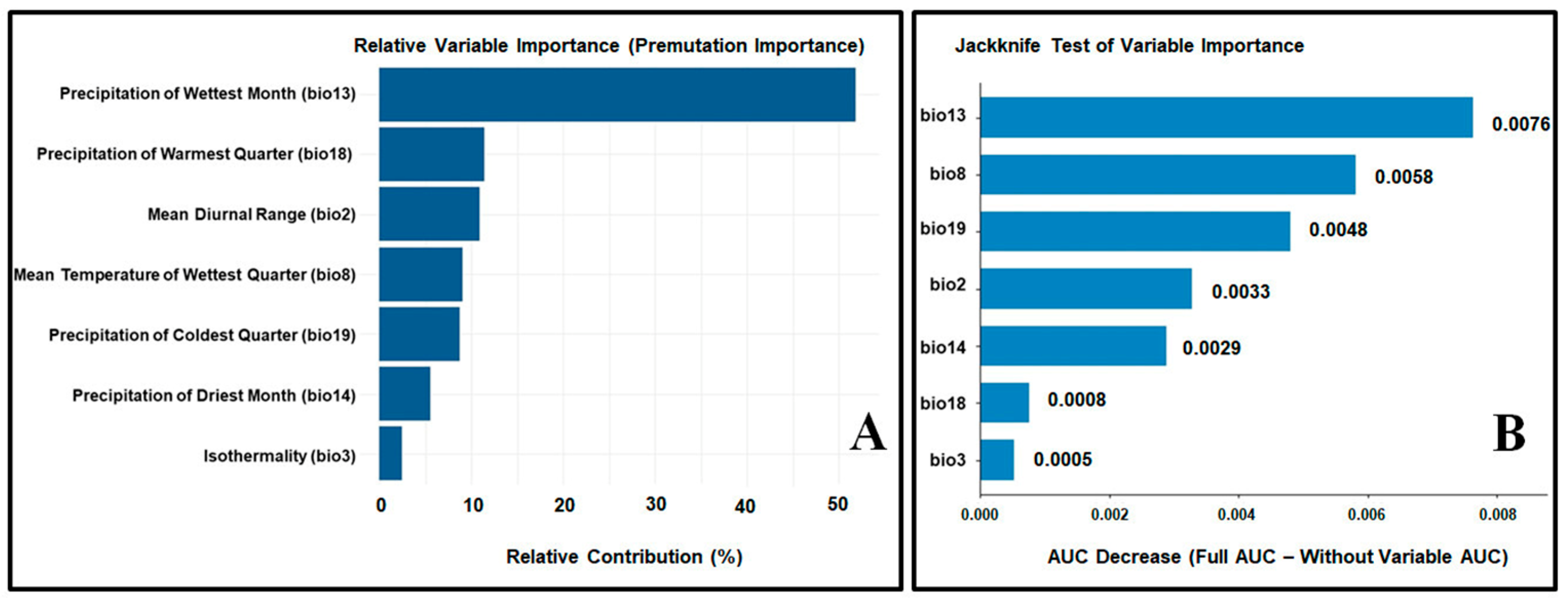
The relative importance of the selected environmental predictors in the optimized MaxEnt model for A. cerana is presented in Figure 4. The permutation importance analysis (Figure 4A) identified precipitation of the wettest month (Bio13) as the most influential predictor, contributing approximately 52% to the overall model performance. This was followed by precipitation of the warmest quarter (Bio18) and mean diurnal range (Bio2), each contributing approximately 11–12%. Mean temperature of the wettest quarter (Bio8) and precipitation of the coldest quarter (Bio19) showed moderate contributions of approximately 9%, whereas precipitation of the driest month (Bio14) and isothermality (Bio3) contributed comparatively less to model performance.
Figure 4.
Relative importance of the selected environmental predictors in the optimized MaxEnt model for Apis cerana. (A) Permutation importance, indicating the relative contribution of each variable to model performance. (B) Jackknife analysis of variable importance, showing the decrease in AUC when each variable is excluded from the model.
The jackknife analysis (Figure 4B), based on the decrease in AUC when individual variables were excluded, further confirmed the importance of precipitation of the wettest month (Bio13), which produced the largest reduction in model performance (AUC decrease = 0.0076). Mean temperature of the wettest quarter (Bio8) was the second most important variable (0.0058), followed by precipitation of the coldest quarter (Bio19; 0.0048) and mean diurnal range (Bio2; 0.0033). Precipitation of the driest month (Bio14; 0.0029) had a moderate influence, while precipitation of the warmest quarter (Bio18; 0.0008) and isothermality (Bio3; 0.0005) had relatively limited independent effects when excluded from the model.
These results indicate that precipitation-related variables, particularly precipitation of the wettest month, played a dominant role in determining the predicted habitat suitability of A. cerana, while temperature-related variables also contributed substantially to model performance.
3.4. Current Habitat Suitability Distribution
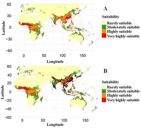
The optimized MaxEnt model predicted that 68.34% of the study area was rarely suitable for A. cerana, while 12.03%, 13.60%, and 6.04% were moderately, highly, and very highly suitable, respectively (Figure 5). Suitable habitats were concentrated mainly in tropical and subtropical regions of South and Southeast Asia, East Asia, and parts of Africa. Highly and very highly suitable areas occurred in distinct geographic clusters rather than being uniformly distributed across the species’ potential range. The map without occurrence records (Figure 5A) illustrates the overall suitability pattern, while the map with occurrence records (Figure 5B) shows that known occurrences were largely associated with predicted suitable areas, particularly those classified as moderately to very highly suitable. Overall, approximately 31.7% of the study area was classified as moderately to very highly suitable. Suitable areas outside the native range indicate potential establishment or invasion-risk zones rather than confirmed occurrences of A. cerana.
Figure 5.
Current habitat suitability for Apis cerana predicted by the optimized MaxEnt model. (A) Predicted habitat suitability without occurrence records overlaid, and (B) predicted habitat suitability with occurrence records (black dots) overlaid.
3.5. Future Projections 2050
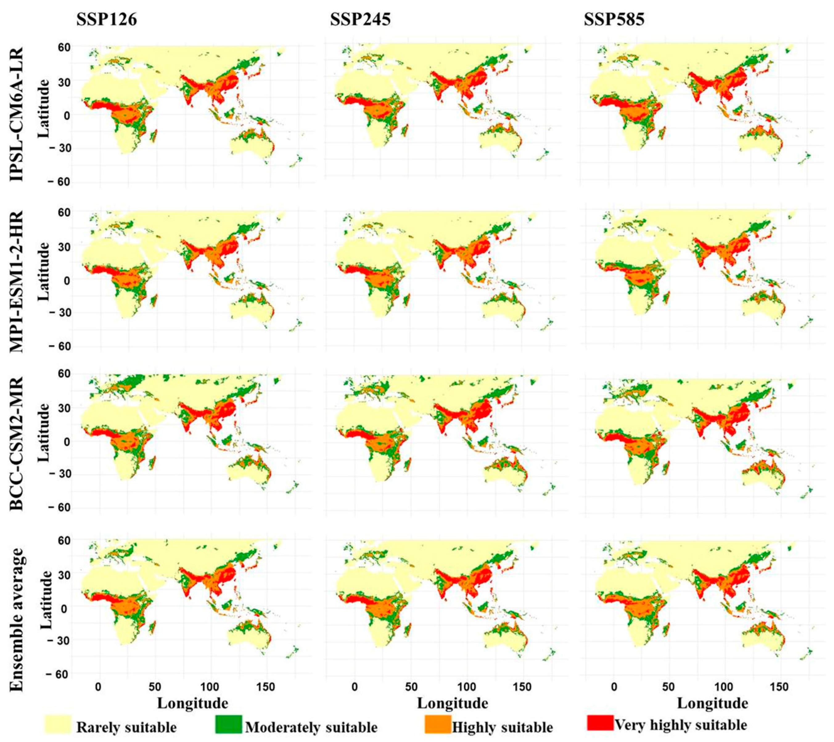
Habitat suitability projections for 2050 under three shared socioeconomic pathway (SSP) scenarios and three global climate models are shown in Figure 6. Across all projections, rarely suitable habitat occupied the largest proportion of the study area, and suitable areas remained concentrated primarily in South and Southeast Asia, with additional areas in East Asia, southern and eastern Africa, and Australia. Under SSP126, rarely suitable habitat ranged from 61.10% under BCC-CSM2-MR to 67.74% under MPI-ESM1-2-HR. Moderately suitable habitat accounted for 12.02–16.96%, highly suitable habitat for 13.14–13.28%, and very highly suitable habitat for 7.10–8.66%. The ensemble projection comprised 65.10% rarely suitable, 14.00% moderately suitable, 13.29% highly suitable, and 7.61% very highly suitable habitat.
Figure 6.
Predicted future habitat suitability of Apis cerana for the year 2050 under three shared socioeconomic pathway scenarios (SSP126, SSP245, and SSP585) across three climate models (IPSL-CM6A-LR, MPI-ESM1-2-HR, and BCC-CSM2-MR).
Under SSP245, rarely suitable habitat ranged from 61.74% to 67.95%, while moderately and highly suitable habitat accounted for 11.89–15.48% and 13.10–13.35%, respectively. Very highly suitable habitat reached 9.04% under IPSL-CM6A-LR and 9.43% under BCC-CSM2-MR, compared with 7.06% under MPI-ESM1-2-HR. The ensemble projection comprised 65.00% rarely suitable, 13.55% moderately suitable, 13.46% highly suitable, and 7.99% very highly suitable habitat. Under SSP585, rarely suitable habitat ranged from 60.49% under BCC-CSM2-MR to 66.33% under MPI-ESM1-2-HR. Moderately suitable habitat accounted for 11.78–15.66%, while highly suitable habitat ranged from 13.20% to 13.91%. Very highly suitable habitat reached 10.76% under IPSL-CM6A-LR and 10.47% under BCC-CSM2-MR, but only 6.82% under MPI-ESM1-2-HR. The ensemble projection comprised 63.68% rarely suitable, 13.39% moderately suitable, 14.77% highly suitable, and 8.17% very highly suitable habitat.
The ensemble projections indicate a gradual shift toward higher suitability classes under increasing emissions. The combined proportion of moderately, highly, and very highly suitable habitat increased from 34.90% under SSP126 to 35.00% under SSP245 and 36.32% under SSP585. This increase was particularly evident in the highly suitable class, which reached 14.77% under SSP585.
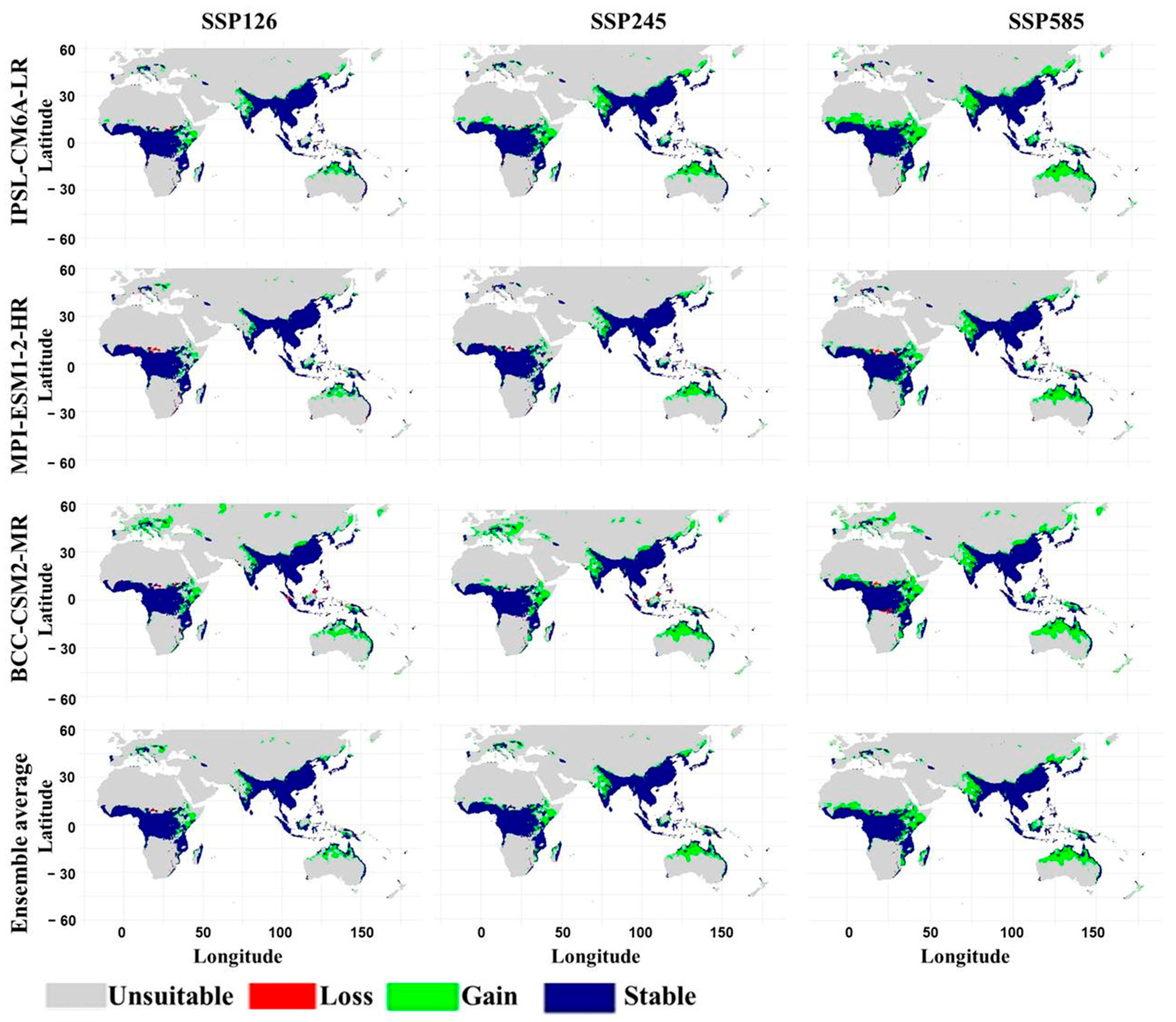
Projected changes in habitat suitability by 2050 relative to the current distribution are shown in Figure 7 (Supplementary Table S2; File S3). Unsuitable areas remained dominant across all model–scenario combinations, while stable habitat accounted for approximately 23% of the study area. Habitat gains generally exceeded losses, with gains increasing under higher-emission scenarios. Under SSP126, unsuitable habitat ranged from 70.22% under BCC-CSM2-MR to 74.15% under MPI-ESM1-2-HR, while stable habitat accounted for 22.61–22.90%. Habitat gain was highest under BCC-CSM2-MR (6.61%), followed by IPSL-CM6A-LR (3.97%) and MPI-ESM1-2-HR (2.68%). Habitat loss ranged from 0.26% under IPSL-CM6A-LR to 0.56% under BCC-CSM2-MR. The ensemble projection comprised 73.02% unsuitable, 22.96% stable, 3.82% gain, and 0.20% loss.
Figure 7.
Projected changes in the habitat suitability of Apis cerana by 2050 under three shared socioeconomic pathway scenarios (SSP126, SSP245, and SSP585) across three global climate models (IPSL-CM6A-LR, MPI-ESM1-2-HR, and BCC-CSM2-MR). Areas are classified as unsuitable, loss, gain, or stable, representing changes relative to the current predicted habitat suitability distribution.
Under SSP245, unsuitable habitat ranged from 69.64% under BCC-CSM2-MR to 74.07% under MPI-ESM1-2-HR, while stable habitat accounted for 22.60–22.88%. BCC-CSM2-MR projected the largest gain (7.19%), whereas MPI-ESM1-2-HR projected the smallest (2.76%). Habitat loss ranged from 0.29% under IPSL-CM6A-LR to 0.57% under BCC-CSM2-MR. The ensemble projection comprised 72.44% unsuitable, 22.98% stable, 4.39% gain, and 0.18% loss. Under SSP585, unsuitable habitat ranged from 68.81% under BCC-CSM2-MR to 72.48% under MPI-ESM1-2-HR, while stable habitat accounted for 22.48–22.92%. BCC-CSM2-MR projected the largest gain (8.03%) and loss (0.69%). IPSL-CM6A-LR projected 6.12% gain and 0.25% loss, whereas MPI-ESM1-2-HR projected 4.36% gain and 0.43% loss. The ensemble projection comprised 70.88% unsuitable, 22.96% stable, 5.96% gain, and 0.21% loss.
Spatially, stable habitat was concentrated mainly within the present suitable range, particularly across South, Southeast, and East Asia, with additional areas in the Australian region. Gains occurred primarily around existing suitable areas, whereas losses were more localized. The ensemble projections showed an increase in habitat gain from 3.82% under SSP126 to 4.39% under SSP245 and 5.96% under SSP585. These results suggest a potential expansion and redistribution of climatically suitable habitat by 2050, although the extent of change differed among climate models. BCC-CSM2-MR generally projected the largest gains, whereas MPI-ESM1-2-HR tended to predict the smallest gains and the largest proportion of unsuitable habitat.
3.6. Future Projections 2070
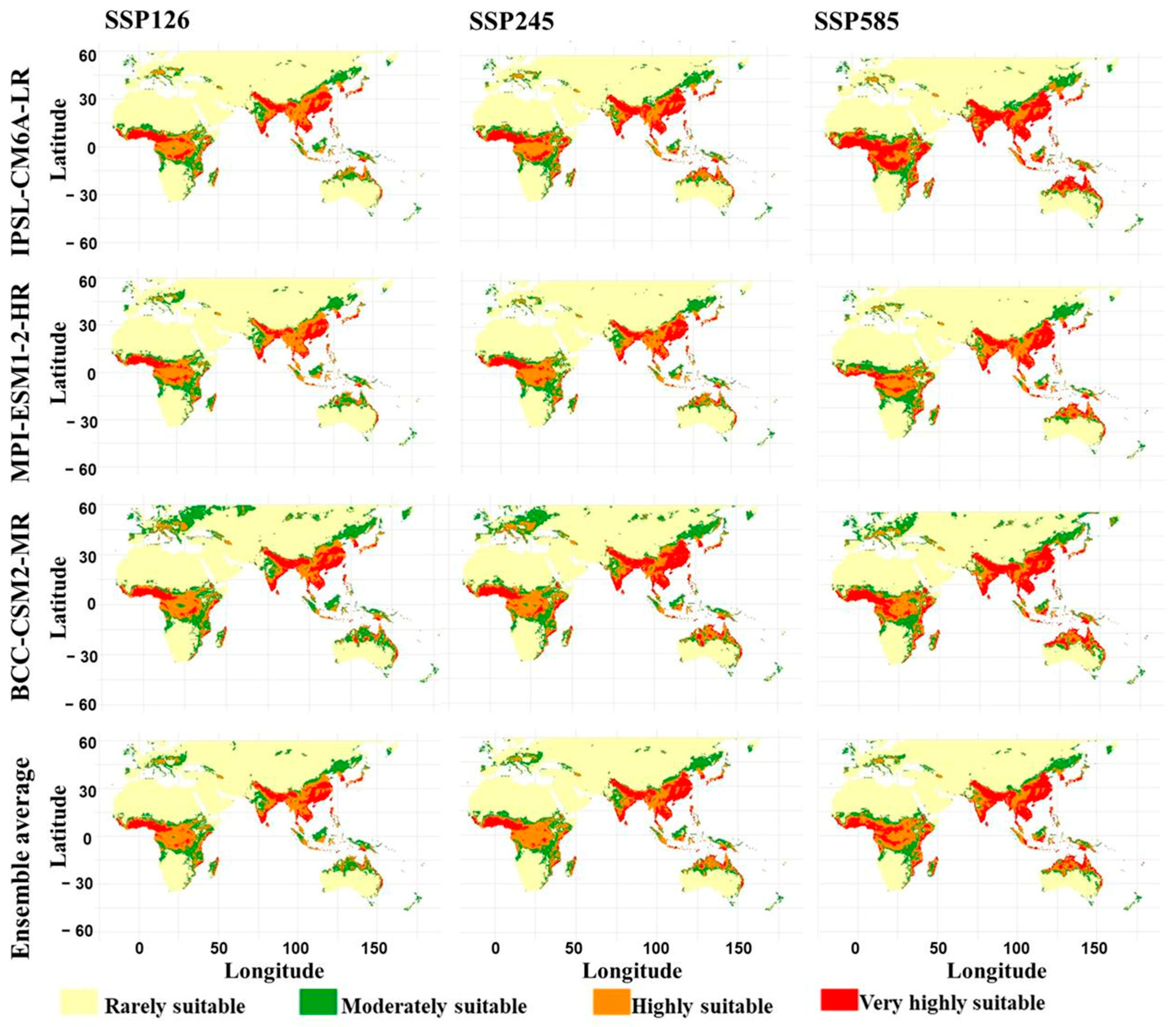
For 2070, suitable habitats were concentrated in South and Southeast Asia, southern China, Japan, and parts of the Indonesian–Australasian region (Figure 8), although their distribution varied among climate models and SSP scenarios. Under SSP585, IPSL-CM6A-LR and BCC-CSM2-MR projected an expansion of areas classified as highly and very highly suitable. Under SSP126, rarely suitable habitat ranged from 60.89% under BCC-CSM2-MR to 67.33% under MPI-ESM1-2-HR. Moderately suitable habitat accounted for 12.33–17.28%, highly suitable habitat for 12.99–13.34%, and very highly suitable habitat for 6.92–8.69%. The ensemble projection comprised 65.18% rarely suitable, 13.90% moderately suitable, 13.30% highly suitable, and 7.62% very highly suitable habitat.
Figure 8.
Predicted future habitat suitability of Apis cerana for the year 2070 under three shared so-cioeconomic pathway scenarios (SSP126, SSP245, and SSP585) across three climate models (IPSL-CM6A-LR, MPI-ESM1-2-HR, and BCC-CSM2-MR).
Under SSP245, rarely suitable habitat accounted for 60.45% under BCC-CSM2-MR, 64.02% under IPSL-CM6A-LR, and 66.88% under MPI-ESM1-2-HR. Moderately suitable habitat ranged from 11.76% to 15.06%, while highly suitable habitat accounted for 13.01–13.67%. Very highly suitable habitat reached 11.21% under IPSL-CM6A-LR and 10.81% under BCC-CSM2-MR. The ensemble projection comprised 63.82% rarely suitable, 13.05% moderately suitable, 13.77% highly suitable, and 9.36% very highly suitable habitat. Under SSP585, rarely suitable habitat declined to 60.93% under IPSL-CM6A-LR and 59.08% under BCC-CSM2-MR, compared with 64.87% under MPI-ESM1-2-HR. Very highly suitable habitat increased to 17.71% under IPSL-CM6A-LR and 14.24% under BCC-CSM2-MR, while MPI-ESM1-2-HR projected 9.87%. The ensemble projection comprised 61.58% rarely suitable, 11.80% moderately suitable, 13.69% highly suitable, and 12.93% very highly suitable habitat.
The ensemble projections indicate increasing suitability under higher-emission scenarios. The combined proportion of moderately, highly, and very highly suitable habitat increased from 34.82% under SSP126 to 36.18% under SSP245 and 38.42% under SSP585. The most pronounced change occurred in the very highly suitable class, which increased from 7.62% to 9.36% and 12.93%, respectively. The increase was particularly marked under IPSL-CM6A-LR, which projected 17.71% very highly suitable habitat under SSP585. Despite the persistence of extensive rarely suitable areas, these results suggest that higher-emission scenarios may increase the availability of climatically favorable habitat by 2070. The magnitude of this change remains dependent on the climate model and SSP scenario.
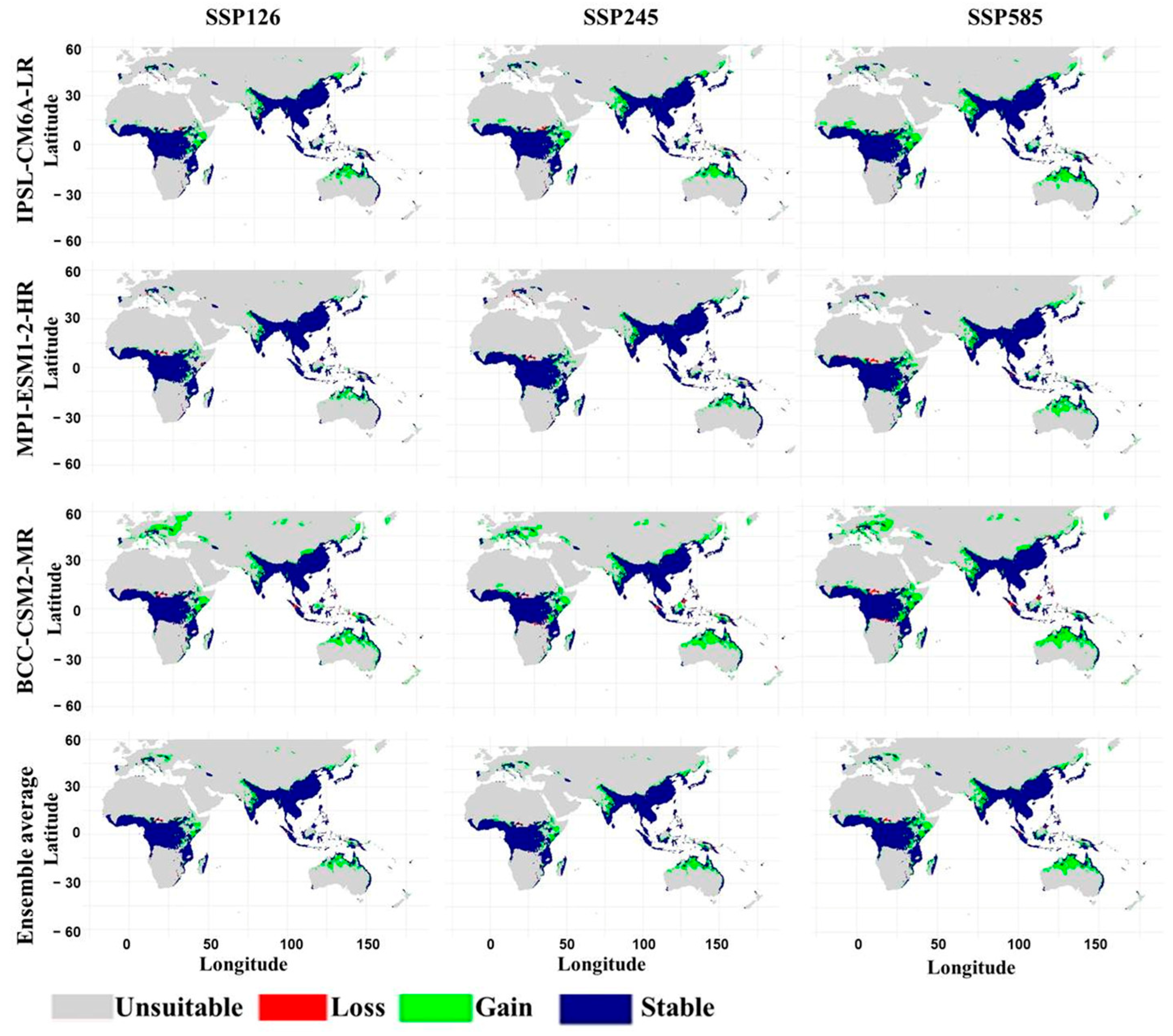
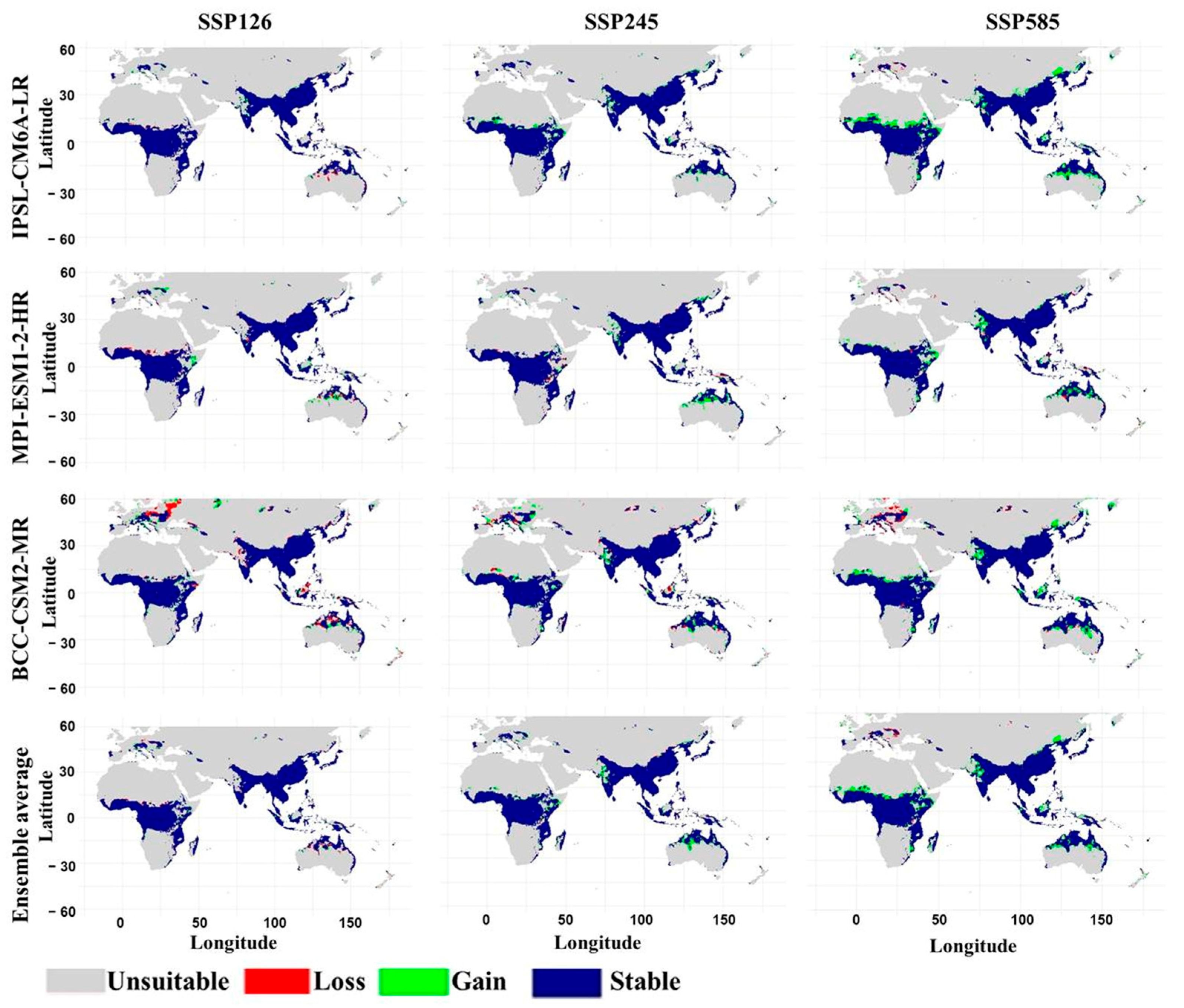
Projected habitat changes by 2070 relative to the current suitability distribution are presented in Figure 9 (Supplementary Table S3; File S3). Unsuitable habitat remained the dominant class, accounting for 70.79–73.91% under SSP126, 68.75–72.96% under SSP245, and 66.55–70.55% under SSP585. Stable habitat accounted for approximately 23% across all projections, whereas habitat gains increased with emissions and losses remained limited. Under SSP126, habitat gain ranged from 2.93% under MPI-ESM1-2-HR to 6.04% under BCC-CSM2-MR. Habitat loss ranged from 0.28% to 0.59%, while stable habitat accounted for 22.58–22.88%. The ensemble projection comprised 73.00% unsuitable, 3.83% gain, 0.21% loss, and 22.96% stable habitat.
Figure 9.
Projected changes in the habitat suitability of Apis cerana by 2070 under three shared socioeconomic pathway scenarios (SSP126, SSP245, and SSP585) across three global climate models (IPSL-CM6A-LR, MPI-ESM1-2-HR, and BCC-CSM2-MR). Areas are classified as unsuitable, loss, gain, or stable, representing changes relative to the current predicted habitat suitability distribution.
Under SSP245, habitat gain ranged from 3.87% under MPI-ESM1-2-HR to 8.09% under BCC-CSM2-MR, while habitat loss ranged from 0.25% to 0.45%. Stable habitat remained relatively consistent at 22.72–22.91%. The ensemble projection comprised 71.01% unsuitable, 5.82% gain, 0.17% loss, and 22.99% stable habitat. Under SSP585, unsuitable habitat ranged from 66.55% under BCC-CSM2-MR to 70.55% under MPI-ESM1-2-HR. Habitat gain reached 10.28% under BCC-CSM2-MR and 10.20% under IPSL-CM6A-LR, compared with 6.28% under MPI-ESM1-2-HR. Habitat loss ranged from 0.21% to 0.47%, while stable habitat remained close to 23%. The ensemble projection comprised 68.08% unsuitable, 8.76% gain, 0.13% loss, and 23.03% stable habitat.
The ensemble projections showed a progressive increase in habitat gain from 3.83% under SSP126 to 5.82% under SSP245 and 8.76% under SSP585. Over the same scenarios, unsuitable habitat declined from 73.00% to 68.08%, while habitat loss remained below 0.59% in all individual model projections. Stable habitat was concentrated mainly within the existing distribution of A. cerana, particularly in parts of South, Southeast, and East Asia, whereas gains occurred primarily along the margins of the current suitable range. These findings indicate a greater potential for habitat expansion than habitat loss by 2070, particularly under SSP585.
Figure 10 illustrates changes in habitat suitability between 2050 and 2070 under the three SSP scenarios and climate models (Supplementary Table S4; File S3). Unsuitable areas remained dominant, while stable habitat accounted for approximately 25–30% of the study area. Habitat gain generally increased with emissions, although the relative magnitudes of gain and loss varied among models. Under SSP126, unsuitable habitat ranged from 69.45% under BCC-CSM2-MR to 73.44% under MPI-ESM1-2-HR. Stable habitat accounted for 24.74–27.28%, while habitat gain ranged from 0.58% to 1.33% and habitat loss from 0.54% to 1.94%. The ensemble projection comprised 72.63% unsuitable, 26.21% stable, 0.58% gain, and 0.57% loss.
Figure 10.
Projected changes in the habitat suitability of Apis cerana between 2050 and 2070 under three shared socioeconomic pathway scenarios (SSP126, SSP245, and SSP585) across three climate models (IPSL-CM6A-LR, MPI-ESM1-2-HR, and BCC-CSM2-MR). Areas are classified as unsuitable, loss, gain, or stable, indicating changes relative to the predicted habitat suitability distribution in 2050.
Under SSP245, unsuitable habitat ranged from 68.12% under BCC-CSM2-MR to 72.82% under MPI-ESM1-2-HR, while stable habitat accounted for 25.09–28.72%. Habitat gain ranged from 1.58% to 2.09%, compared with 0.14–1.07% loss. The ensemble projection comprised 70.93% unsuitable, 27.13% stable, 1.69% gain, and 0.25% loss. Under SSP585, unsuitable habitat ranged from 66.00% under BCC-CSM2-MR to 70.45% under MPI-ESM1-2-HR, while stable habitat accounted for 26.51–29.54%. Habitat gain reached 4.39% under IPSL-CM6A-LR, 3.49% under BCC-CSM2-MR, and 2.47% under MPI-ESM1-2-HR. Habitat loss ranged from 0.27% to 0.96%. The ensemble projection comprised 67.87% unsuitable, 28.57% stable, 3.22% gain, and 0.34% loss.
Spatially, stable habitat remained concentrated in parts of South, Southeast, and East Asia. Habitat gains became more extensive under SSP245 and SSP585, whereas losses were generally more localized. The ensemble projections showed that habitat gain increased from 0.58% under SSP126 to 1.69% under SSP245 and 3.22% under SSP585. Ensemble habitat loss remained below 1% across all scenarios, although individual model projections showed greater variation under SSP126. Overall, the results indicate increasingly pronounced changes in the spatial distribution of climatically suitable habitat between 2050 and 2070 under higher-emission scenarios, with SSP585 showing the greatest projected gain and SSP126 the smallest change.
MESS analysis revealed substantial climatic novelty in the projected distribution of A. cerana. By 2050 (Supplementary Figure S4; File S2), negative MESS values covered 42.63%, 42.93%, and 42.86% of the study area under SSP126, SSP245, and SSP585, respectively, while the overall ensemble reached 43.45%. By 2070 (Supplementary Figure S5; File S2), climatic novelty increased from 42.59% under SSP126 to 43.54% under SSP245 and 45.40% under SSP585, with the overall ensemble reaching 45.04%. Novel conditions were concentrated mainly in southern Africa, the Indian subcontinent, East and Southeast Asia, and parts of northern Eurasia. The increasing proportion of negative MESS values under stronger emissions indicates greater climatic extrapolation risk, particularly under SSP585.
4. Discussion
The selection of the LQH feature class combination with a low regularization multiplier (RM = 1) as the optimal Maximum Entropy (MaxEnt) configuration suggests that a relatively flexible model structure was necessary to capture the complex, nonlinear ecological relationships governing the spatial distribution of A. cerana, while maintaining an appropriate balance between model fit and parsimony [28,29]. The higher ΔAICc values at larger regularization multipliers suggest that excessive penalization may have oversmoothed important environmental responses [30]. Consistent performance across spatially structured cross-validation further supports the model’s robustness and transferability across geographic areas [31,32].
The combined evaluation metrics indicate that the model achieved good discriminatory ability and maintained reliable predictive performance across the spatially independent validation folds [33,34]. In particular, the strong calibration and consistency indicated by CBI provide further support for the model’s ability to correctly rank environmentally suitable conditions using presence-only data [35]. The high sensitivity and correspondingly low omission rate demonstrate that the optimized model successfully captured the majority of known A. cerana occurrences, which is particularly important when developing habitat suitability maps intended to identify potentially suitable areas [36]. Although moderate specificity suggests some background areas were also classified as suitable, this is expected in presence-background modelling, as environmentally suitable areas may remain unoccupied or undocumented because of dispersal limitations, or biotic interactions [37]. Low variability among spatial folds indicates stable predictions and limited influence of spatial autocorrelation, supporting the model’s reliability for ecological interpretation and conservation planning [38].
The response curves indicate that A. cerana habitat suitability is shaped by complex interactions between seasonal moisture and thermal conditions. Positive responses to precipitation during the wettest month and the warmest and coldest quarters highlight the importance of adequate seasonal moisture for maintaining floral resources, foraging, and colony development [4,6], whereas the negative response to precipitation during the driest month suggests that dry-season rainfall may have a different ecological influence due to interactions with vegetation and microclimate. Thermal responses further indicate a preference for relatively stable daily temperatures, as suitability declined with increasing diurnal temperature range and varied with isothermality [4]. The positive association with mean temperature during the wettest quarter reflects the species’ adaptation to warm, humid conditions that favor brood development, reproduction, and foraging [6]. These patterns suggest that the climatic niche of A. cerana is primarily characterized by adequate seasonal moisture, warm conditions during wet periods, and moderate thermal variability.
The variable importance analyses further confirm that precipitation-related factors are the principal determinants of predicted habitat suitability, with precipitation during the wettest month emerging as the most influential predictor. This finding underscores the critical ecological role of peak seasonal moisture in maintaining vegetation productivity, floral resource availability, and colony nutrition [4,7]. The importance of precipitation during other seasonal periods indicates that habitat suitability is influenced not only by peak rainfall but also by the broader seasonal distribution of moisture. Temperature-related predictors, particularly mean temperature during the wettest quarter and mean diurnal temperature range, also contributed meaningfully to model performance, emphasizing the role of thermal conditions in regulating bee activity, development, and physiological functioning [4,6]. Jackknife analysis confirmed the importance of major precipitation and temperature predictors, while differences in variable contributions suggest overlapping environmental information. Overall, A. cerana distribution is primarily influenced by seasonal moisture availability and thermal stability, with changes in wet-season precipitation potentially altering climatically suitable habitats [4,7].
The habitat suitability model revealed pronounced spatial heterogeneity in the potential distribution of A. cerana, with favorable conditions concentrated mainly in tropical and subtropical regions of South, Southeast, and East Asia, broadly matching the species’ known biogeographic range and areas where it is widely used in apiculture [3,4]. The predicted distribution also agrees with the recent modeling study [4], which demonstrated that climatic conditions strongly influence the distribution of A. cerana in China. While [4] focused on China and assessed potential distribution under climate-change scenarios, the present study considers a broader geographic extent and therefore provides a wider assessment of the spatial distribution of climatically suitable habitats. Any differences between the suitability patterns identified here and those reported by [4] may be attributable to differences in geographic extent, occurrence data, environmental predictors, and modeling approaches. In particular, the broader spatial extent of the present analysis may capture climatic combinations occurring outside China that were not represented in the regional analysis of [4]. The concentration of highly suitable areas within specific geographic zones suggests that A. cerana depends on particular climatic combinations, including adequate seasonal moisture, warm conditions during wet periods, and relatively stable thermal environments. Although most of the study area showed low suitability, localized areas of moderate to very high suitability suggest that favorable habitats are geographically limited and concentrated in warm, humid environments that support colony development, activity, and floral resources [3,4]. The close correspondence between known occurrences and predicted suitable areas further supports the model’s ability to capture environmental conditions consistent with the realized distribution of A. cerana.
The identification of suitable habitats beyond the established range, including parts of Africa, indicates the presence of climatically favorable areas outside the species’ well-documented range. These predictions should not be considered evidence of established populations but rather areas that could potentially support A. cerana if dispersal, introduction, and other ecological requirements occur [3]. Such areas may therefore be important for assessing potential climatic suitability expansion, accidental introduction, and biological invasion. The suitability map therefore provides a spatial baseline that complements previous regional modeling studies and contributes broader ecological insight into the climatic conditions potentially supporting A. cerana, while highlighting that climatic suitability alone cannot fully explain the species’ realized distribution.
Future projections suggest that A. cerana will experience a moderate net expansion and spatial redistribution of climatically suitable habitat by 2050, particularly under higher-emission scenarios, while much of the current suitable range is expected to persist as stable habitat. Stable suitability remains concentrated across South, Southeast, and East Asia, where the species is widely used in apiculture, highlighting these regions as potential climatic refugia and conservation priorities [3,6], with additional persistence projected in parts of Australia. Increased representation of higher-suitability classes and newly suitable areas under stronger warming may reflect the species’ climatic plasticity and thermal tolerance [4], with newly suitable habitats generally occurring along the margins of the current distribution and potentially facilitating expansion toward cooler latitudes or higher elevations [3]. However, the relatively modest changes in total suitable area and the coexistence of localized gains and contractions indicate heterogeneous responses to climate change. Differences among GCMs introduce uncertainty in the magnitude and spatial configuration of projected changes, although the three-model ensemble across multiple SSPs provides greater confidence in the overall patterns [32]. Importantly, areas projected as suitable outside the established range, including parts of Africa and other regions, represent climatic potential rather than confirmed establishment, as future expansion may be constrained by dispersal limitations, habitat fragmentation, land-use and land-cover changes, interspecific competition, particularly with A. mellifera, and host–parasite dynamics [3,6,17,39]. Overall, climate change is projected to moderately increase the potential range of A. cerana by 2050, while its established tropical and subtropical range remains central to future monitoring and conservation management.
Projections for 2070 indicate a predominantly stable-to-expanding pattern in the potential climatic distribution of A. cerana, with the magnitude of change increasing under stronger greenhouse gas forcing, particularly SSP585. Suitable habitats remain concentrated across South, Southeast, and East Asia, including southern China and Japan, as well as parts of the Indonesian–Australasian region, where the species is widely used in apiculture, indicating strong macroclimatic persistence and the potential for long-term climatic refugia [4,6]. Compared with 2050, the projections suggest greater habitat gains and comparatively limited, localized losses, resulting in a gradual net expansion and spatial redistribution of suitable conditions rather than widespread contraction. Newly suitable areas are projected mainly along the margins of the current range, potentially facilitating expansion toward cooler latitudinal or elevational environments [3], while substantial portions of the broader landscape remain unsuitable, indicating spatially selective rather than uniform expansion. The greater availability of highly suitable thermal and moisture conditions under stronger warming may reflect considerable macroclimatic resilience of A. cerana, although responses remain spatially heterogeneous. Consistency in major stable areas across models increases confidence in the persistence of key climatic refugia, whereas differences in the extent and location of newly suitable areas highlight uncertainty in the magnitude and spatial configuration of future changes. Importantly, areas projected as suitable should be interpreted as potential climatic habitat rather than guaranteed future occupancy or colonization. Overall, the ensemble projections support a gradual increase and redistribution of climatically suitable habitat between 2050 and 2070, particularly under stronger climate forcing, while the persistence of major suitable areas indicates substantial macroclimatic resilience of A. cerana.
The presence of potential terrestrial pathways for the range expansion and dispersal of A. cerana within the study area may facilitate its direct spread into climatically suitable areas through swarming, the primary natural mechanism of colony reproduction. Additionally, anthropogenic activities, such as international trade, may facilitate the redistribution of A. cerana beyond its native range, as demonstrated by the detection of A. florea [40,41,42,43] and A. dorsata [44] beyond Asia. Therefore, regions projected to become increasingly suitable, especially major trade and transport hubs, may require continued surveillance and strengthened biosecurity to detect and intercept incoming swarms before establishment. In this context, the suitability patterns identified in this study can serve as a spatial basis for prioritizing surveillance efforts, particularly in areas where climatic suitability overlaps with major ports, airports, agricultural production areas, or other potential entry and establishment pathways. Proactive monitoring could include targeted inspection of incoming cargo and vessels, early detection of swarms, and rapid reporting and response in areas identified as climatically suitable. Such measures would be particularly important because early intervention may prevent establishment before populations become widespread and more difficult to eradicate. Thus, our projections should not only be interpreted as estimates of future habitat suitability but also as an early-warning framework for identifying areas where invasion risk may increase under changing climatic conditions.
The projected distribution also has implications for apiculture and pollination-service management. Areas becoming climatically suitable may provide opportunities for the expansion or establishment of Apis populations that could contribute to local pollination services, but these potential benefits should be considered alongside the risks associated with introducing or facilitating the spread of non-native populations. In regions where suitable conditions are projected to increase, beekeeping and agricultural stakeholders could use these predictions to anticipate changes in the availability and distribution of pollinators, identify areas where pollination services may become more feasible or reliable, and plan apiary placement and management accordingly. Conversely, where range expansion could involve non-native or potentially invasive populations, management strategies should emphasize prevention of unintended translocation and avoid practices that could facilitate further spread. Integrating climatic suitability with apicultural activity, crop distributions, and transport networks could therefore help distinguish areas where projected suitability may support pollination-service planning from those where enhanced biosecurity and invasive-species surveillance should take priority. Collectively, these applications demonstrate how climate-based distribution projections can support both proactive invasion-risk assessment and more informed, spatially targeted management of apiculture and pollination services.
The MESS results highlight an important limitation when interpreting future habitat suitability for A. cerana. Climatic novelty indicates that parts of the projected range may experience environmental conditions not adequately represented by the species’ current occurrence data. This is particularly relevant under stronger climate forcing, where greater climatic divergence may reduce the reliability of extrapolated suitability estimates. The MESS findings emphasize that projected range expansions should not be interpreted solely as evidence of future habitat suitability, but alongside the degree of environmental novelty and associated extrapolation uncertainty.
5. Conclusions
This study demonstrates that an optimized MaxEnt framework provides a robust basis for assessing the current climatic suitability and future range dynamics of A. cerana. The LQH feature class with a regularization multiplier of 1 achieved a balance between predictive performance, flexibility, and parsimony, with consistent performance across spatially structured cross-validation folds supporting model robustness and geographic transferability. Climatic suitability was driven primarily by precipitation, particularly precipitation during the wettest month, together with key thermal variables, indicating that A. cerana is strongly associated with warm, humid environments with adequate seasonal moisture and relatively stable thermal conditions. Current highly suitable habitats were concentrated across South, Southeast, and East Asia, consistent with the species’ known distribution, while additional climatically suitable areas represent potential rather than established populations. Future projections suggest potential changes in climatic suitability through 2050 and 2070, with the magnitude and spatial extent of projected changes varying among climate scenarios. Although projections indicate potential gains in climatically suitable areas, particularly under SSP585, these results should be interpreted cautiously due to the substantial climatic novelty identified by the MESS analysis. Importantly, these projections represent potential climatic suitability rather than confirmed future colonization or range expansion, which may be constrained or facilitated by ecological and anthropogenic factors not explicitly incorporated into the model. The exclusion of additional non-climatic factors, including dispersal limitations, land-use change, habitat fragmentation, biotic interactions, and human-mediated transport, represents a significant limitation of this study. These factors were not incorporated because spatially explicit datasets with consistent coverage across the entire study area under both current and future conditions were not readily available at a comparable spatial resolution. These findings provide a valuable baseline for climate-informed conservation and proactive monitoring of potential expansions in climatic suitability and associated invasion risks.
Supplementary Materials
The following supporting information can be downloaded at: https://www.mdpi.com/article/10.3390/agriculture16212337/s1, File S1: 870 records used in the study, File S2: Supplementary Figures, and File S3: Supplementary Tables.
Author Contributions
Conceptualization, A.A.A., M.I.I., M.K., H.F.A.-S. and S.A.A.; methodology, A.A.A., H.F.A.-S., M.I.I., M.K. and S.A.A.; validation, A.A.A., H.F.A.-S., M.I.I., M.K. and S.A.A.; formal analysis, H.F.A.-S., M.I.I., M.K. and S.A.A.; investigation, H.F.A.-S., M.I.I., M.K. and S.A.A.; data curation, H.F.A.-S. and S.A.A.; writing—original draft preparation, A.A.A., H.F.A.-S., M.I.I., M.K. and S.A.A.; writing—review and editing, A.A.A., H.F.A.-S., M.I.I., M.K. and S.A.A.; funding acquisition, A.A.A. All authors have read and agreed to the published version of the manuscript.
Funding
Princess Nourah bint Abdulrahman University Researchers Supporting Project (number PNURSP2026R37), Princess Nourah bint Abdulrahman University, Riyadh, Saudi Arabia.
Data Availability Statement
The data supporting the findings of this study are included within the article and its supplementary materials. Additional data are available from the corresponding author upon reasonable request.
Acknowledgments
The authors acknowledge the support from Princess Nourah bint Abdulrahman University Researchers Supporting Project (number PNURSP2026R37), Princess Nourah bint Abdulrahman University, Riyadh, Saudi Arabia.
Conflicts of Interest
The authors declare no conflicts of interest.
Abbreviations
The following abbreviations are used in this manuscript:
| MaxEnt | Maximum Entropy |
| SSP | Shared Socioeconomic Pathway |
| AUC | The Area Under the Curve |
| TSS | True Skill Statistic |
References
- Ollerton, J.; Winfree, R.; Tarrant, S. How many flowering plants are pollinated by animals? Oikos 2011, 120, 321–326. [Google Scholar] [CrossRef] [Scilit]
- Hung, K.L.J.; Kingston, J.M.; Albrecht, M.; Holway, D.A.; Kohn, J.R. The worldwide importance of honey bees as pollinators in natural habitats. Proc. R. Soc. B 2018, 285, 20172140. [Google Scholar] [CrossRef] [Scilit] [PubMed]
- Koetz, A.H. Ecology, behaviour and control of Apis cerana with a focus on relevance to the Australian incursion. Insects 2013, 4, 558–592. [Google Scholar] [CrossRef] [Scilit] [PubMed]
- Chen, Y.; Mao, X.; Zhao, Z.; Zhang, S. Predicting impact of climate change on Eastern honeybee (Apis cerana) distribution in China using Biomod2 ensemble model. Agriculture 2026, 16, 534. [Google Scholar] [CrossRef] [Scilit]
- Oldroyd, B.P.; Nanork, P. Conservation of Asian honey bees. Apidologie 2009, 40, 296–312. [Google Scholar] [CrossRef] [Scilit]
- Oldroyd, B.P.; Wongsiri, S. Asian Honey Bees: Biology, Conservation, and Human Interactions; Harvard University Press: Cambridge, MA, USA, 2009. [Google Scholar]
- Chouangthavy, B. Crop pollination by native honey bees (Apis cerana) at risk due to agricultural intensification. Arthropod-Plant Interact. 2025, 19, 89. [Google Scholar] [CrossRef] [Scilit]
- Lin, Z.; Page, P.; Li, L.; Qin, Y.; Zhang, Y.; Hu, F.; Neumann, P.; Zheng, H.; Dietemann, V. Go east for better honey bee health: Apis cerana is faster at hygienic behavior than A. mellifera. PLoS ONE 2016, 11, e0162647. [Google Scholar] [CrossRef] [Scilit] [PubMed]
- Partap, L.; Verma, L.R. Asian bees and beekeeping: Issues and initiatives. In Proceedings of the 4th Asian Apiculture Association International Conference 1998, Kathmandu, Nepal; Oxford & IBH Publishing Co. Pvt. Ltd.: Delhi, India, 1998; pp. 23–28. [Google Scholar]
- Xue, Y.; Zhao, W.; Meng, Q.; Yang, L.; Zhi, D.; Guo, Y.; Yue, D.; Tian, Y.; Dong, K. Combined toxic effects of lead and glyphosate on Apis cerana cerana. Insects 2024, 15, 644. [Google Scholar] [CrossRef] [Scilit] [PubMed]
- Manchikatla, S.; Amritha, V.S.; Anith, K.N.; Vijayasree, V.; Kumaranag, K.M. Current Perspectives on Bacterial and Viral Brood Diseases of Apis cerana indica in India: Prevalence, Diagnostics, and Management Strategies. Indian J. Microbiol. 2026, 66, 1135–1149. [Google Scholar] [CrossRef] [Scilit] [PubMed]
- Rafferty, N.E. Effects of global change on insect pollinators: Multiple drivers lead to novel communities. Curr. Opin. Insect Sci. 2017, 23, 22–27. [Google Scholar] [CrossRef] [Scilit] [PubMed]
- Gómez-Ruiz, E.P.; Lacher, T.E., Jr. Climate change, range shifts, and the disruption of a pollinator-plant complex. Sci. Rep. 2019, 9, 14048. [Google Scholar] [CrossRef] [Scilit] [PubMed]
- Lazar, J.; Prasad, S.; Barboni, D.; Das, L.; Kumaresan, V.; Anupama, K. Diversity matters: Diet of Apis cerana in southeast India includes one consistently occurring and several seasonally available floral sources. Palynology 2024, 48, 2255990. [Google Scholar] [CrossRef] [Scilit]
- Guo, L.; Zhang, Y.; Wang, J.; Yu, D.; Wu, M.; Guo, Y. Environmental temperature modulates olfactory reception in Apis cerana cerana (Hymenoptera: Apidae). Can. Entomol. 2025, 157, e10. [Google Scholar] [CrossRef] [Scilit]
- Tan, K.; Meixner, M.D.; Fuchs, S.; Zhang, X.; He, S.; Kandemir, I.; Sheppard, W.S.; Koeniger, N. Geographic distribution of the eastern honeybee, Apis cerana (Hymenoptera: Apidae), across ecological zones in China: Morphological and molecular analyses. Syst. Biodivers. 2006, 4, 473–482. [Google Scholar] [CrossRef] [Scilit]
- Elith, J.; Leathwick, J.R. Species distribution models: Ecological explanation and prediction across space and time. Annu. Rev. Ecol. Evol. Syst. 2009, 40, 677–697. [Google Scholar] [CrossRef] [Scilit]
- Sillero, N. What does ecological modelling model? A proposed classification of ecological niche models based on their underlying methods. Ecol. Modell. 2011, 222, 1343–1346. [Google Scholar] [CrossRef] [Scilit]
- Blair, M.E.; Le, M.D.; Xu, M. Species distribution modeling to inform transboundary species conservation and management under climate change: Promise and pitfalls. Front. Biogeogr. 2022, 14, e54662. [Google Scholar] [CrossRef] [Scilit]
- Abou-Shaara, H.F. Using maximum entropy algorithm to analyze changes in the distribution of the stingless bees, Tetragonisca angustula (Latreille, 1811), in response to future climatic conditions. J. Entomol. Res. Soc. 2024, 26, 281–295. [Google Scholar] [CrossRef] [Scilit]
- Khan, T.U.; Luan, X.; Nabi, G.; Raza, M.F.; Iqbal, A.; Khan, S.N.; Hu, H. Forecasting the impact of climate change on Apis dorsata (Fabricius, 1793) habitat and distribution in Pakistan. Insects 2025, 16, 289. [Google Scholar] [CrossRef] [Scilit] [PubMed]
- Nasser, M.; Abou-Shaara, H.; AlKhalaf, A.A.; AlAshaal, S.; Hosni, E. Modeling the potential range expansion of Hypotrigona gribodoi (stingless bees) in Africa: Assessing climate change impacts and habitat suitability using Maxent and GIS. Int. J. Trop. Insect Sci. 2025, 45, 1771–1781. [Google Scholar] [CrossRef] [Scilit]
- Fick, S.E.; Hijmans, R.J. WorldClim 2: New 1-km spatial resolution climate surfaces for global land areas. Int. J. Climatol. 2017, 37, 4302–4315. [Google Scholar] [CrossRef] [Scilit]
- Booth, T.H. Checking bioclimatic variables that combine temperature and precipitation data before their use in species distribution models. Austral Ecol. 2022, 47, 1506–1514. [Google Scholar] [CrossRef] [Scilit]
- Hosni, E.M.; Al-Khalaf, A.A.; Nasser, M.G.; Abou-Shaara, H.F.; Radwan, M.H. Modeling the potential global distribution of honeybee pest, Galleria mellonella under changing climate. Insects 2022, 13, 484. [Google Scholar] [CrossRef] [Scilit] [PubMed]
- Abou-Shaara, H.F.; Al-Khalaf, A.A. Climate-Driven Range Dynamics and Spatial Reorganization of the Oriental Hornet (Vespa orientalis) in the Western Palearctic Under Current and Future Scenarios. Diversity 2026, 18, 290. [Google Scholar] [CrossRef] [Scilit]
- Phillips, S.J.; Anderson, R.P.; Dudík, M.; Schapire, R.E.; Blair, M.E. Opening the black box: An open-source release of Maxent. Ecography 2017, 40, 887–893. [Google Scholar] [CrossRef] [Scilit]
- Warren, D.L.; Seifert, S.N. Ecological niche modeling in Maxent: The importance of model complexity and the performance of model selection criteria. Ecol. Appl. 2011, 21, 335–342. [Google Scholar] [CrossRef] [Scilit] [PubMed]
- Muscarella, R.; Galante, P.J.; Soley-Guardia, M.; Boria, R.A.; Kass, J.M.; Uriarte, M.; Anderson, R.P. ENMeval: An R package for conducting spatially independent evaluations and estimating optimal model complexity for Maxent ecological niche models. Methods Ecol. Evol. 2014, 5, 1198–1205. [Google Scholar] [CrossRef] [Scilit]
- Merow, C.; Smith, M.J.; Silander, J.A., Jr. A practical guide to MaxEnt for modeling species’ distributions: What it does, and why inputs and settings matter. Ecography 2013, 36, 1058–1069. [Google Scholar] [CrossRef] [Scilit]
- Roberts, D.R.; Bahn, V.; Ciuti, S.; Boyce, M.S.; Elith, J.; Guillera-Arroita, G.; Hauenstein, S.; Lahoz-Monfort, J.J.; Schröder, B.; Thuiller, W.; et al. Cross-validation strategies for data with temporal, spatial, hierarchical, or phylogenetic structure. Ecography 2017, 40, 913–929. [Google Scholar] [CrossRef] [Scilit]
- Koldasbayeva, D.; Zaytsev, A. Foundation for unbiased cross-validation of spatio-temporal models for species distribution modeling. Ecol. Inform. 2025, 92, 103521. [Google Scholar] [CrossRef] [Scilit]
- Fielding, A.H.; Bell, J.F. A review of methods for the assessment of prediction errors in conservation presence/absence models. Environ. Conserv. 1997, 24, 38–49. [Google Scholar] [CrossRef] [Scilit]
- Allouche, O.; Tsoar, A.; Kadmon, R. Assessing the accuracy of species distribution models: Prevalence, kappa and the true skill statistic (TSS). J. Appl. Ecol. 2006, 43, 1223–1232. [Google Scholar] [CrossRef] [Scilit]
- Hirzel, A.H.; Le Lay, G.; Helfer, V.; Randin, C.; Guisan, A. Evaluating the ability of habitat suitability models to predict species presences. Ecol. Model. 2006, 199, 142–152. [Google Scholar] [CrossRef] [Scilit]
- Liu, C.; White, M.; Newell, G. Selecting thresholds for the prediction of species occurrence with presence-only data. J. Biogeogr. 2013, 40, 778–789. [Google Scholar] [CrossRef] [Scilit]
- Phillips, S.J.; Anderson, R.P.; Schapire, R.E. Maximum entropy modeling of species geographic distributions. Ecol. Model. 2006, 190, 231–259. [Google Scholar] [CrossRef] [Scilit]
- Radosavljevic, A.; Anderson, R.P. Making better Maxent models of species distributions: Complexity, overfitting and evaluation. J. Biogeogr. 2014, 41, 629–643. [Google Scholar] [CrossRef] [Scilit]
- Abou-Shaara, H.F. Competition for resources: What factors lead honey bees to outcompete other insect competitors? Acta Oecol. 2025, 127, 104077. [Google Scholar] [CrossRef] [Scilit]
- Silva, D.P.; Castro, A.C.F.; Vilela, B.; Ong, X.R.; Thomas, J.C.; Alqarni, A.S.; Engel, M.S.; Ascher, J.S. Colonizing the east and the west: Distribution and niche properties of a dwarf Asian honey bee invading Africa, the Middle East, the Malay Peninsula, and Taiwan. Apidologie 2020, 51, 75–87. [Google Scholar] [CrossRef] [Scilit]
- Abou-Shaara, H.F.; Mahfouz, H.M.; Owayss, A.A. Species distribution modeling of potential invasion of dwarf honey bee, Apis florea Fab., to Africa and Europe after occurrence in Egypt in view of climatic changes. J. Plant Prot. Pathol. 2021, 12, 609–614. [Google Scholar] [CrossRef] [Scilit]
- Uzunov, A.; Koeniger, G.; Scheiner, R.; Galea, T.; Koeniger, N. Apis florea in Malta! A Short Visit or a Permanent Stay? Bee World 2025, 102, 30–35. [Google Scholar] [CrossRef] [Scilit]
- Smith-Pardo, A.H.; Kumar, S.; Fowler, G.A. United States port interceptions and predicted climate suitability of the red dwarf honeybee, Apis florea (Hymenoptera: Apidae), with notes on its identification. Apidologie 2021, 52, 915–932. [Google Scholar] [CrossRef] [Scilit]
- Ramirez, J.L.; Tembrock, L.R.; Zink, F.A.; Fife, A.; Gilligan, T.M.; Chen, Y.; Evans, J.D.; Mottern, J.; Smith-Pardo, A.H.; Ochoa, R. Interception of an Apis dorsata swarm with Tropilaelaps mercedesae and Kuzinia morsei mites on a cargo vessel inbound to the United States. Front. Insect Sci. 2026, 6, 1829350. [Google Scholar] [CrossRef] [Scilit] [PubMed]
Disclaimer/Publisher’s Note: The statements, opinions and data contained in all publications are solely those of the individual author(s) and contributor(s) and not of MDPI and/or the editor(s). MDPI and/or the editor(s) disclaim responsibility for any injury to people or property resulting from any ideas, methods, instructions or products referred to in the content. |
© 2026 by the authors. Licensee MDPI, Basel, Switzerland. This article is an open access article distributed under the terms and conditions of the Creative Commons Attribution (CC BY) license.