


Abstract
Accurate prediction of multiple environmental factors in laying hen houses is essential for maintaining optimal rearing conditions, yet the strong nonlinear coupling among temperature, relative humidity, CO2, and PM2.5 concentrations, combined with complex temporal dependencies, poses significant challenges for conventional forecasting models. To address these challenges, this study proposes a collaborative multi-environmental factor prediction framework that integrates adaptive Kalman filtering (AKF), a dynamic attention mechanism, and a convolutional neural network–long short-term memory (CNN-LSTM) architecture. The AKF preprocesses raw sensor data to suppress noise while preserving salient transient features; the attention mechanism adaptively weights time steps exhibiting rapid changes across environmental variables; and the CNN-LSTM model performs synchronized high-precision forecasting of all target factors. Experimental validation using real-world summer data from commercial layer hen houses demonstrates that the proposed model achieves superior predictive accuracy across all four environmental variables, effectively capturing both short-term fluctuations and long-term temporal dependencies. These findings indicate that the AKF-Attention-CNN-LSTM framework can serve as a reliable tool for precise environmental regulation, providing actionable forecasts to support automated climate control in laying hen production systems.
1. Introduction
Amid the rapid intensification of China’s livestock industry, the laying hen sector is transitioning toward large-scale, intelligent operations [1]. However, with operational scale expansion, deficiencies in environmental control technology have become increasingly evident. A laying hen house constitutes a complex dynamic system shaped by multiple interacting factors—including temperature, relative humidity, air velocity, noxious gases, and particulate matter—where environmental quality directly influences hen health and productive performance [2,3,4,5,6,7].
Empirical evidence indicates that suboptimal environmental conditions in laying hen houses not only reduce feed intake and egg production but also precipitate severe respiratory disorders, culminating in substantial economic losses [8,9,10,11]. Consequently, the precise forecasting of dynamic variations in multiple environmental parameters within laying hen houses—and the subsequent implementation of targeted environmental control strategies—is critical for maintaining and enhancing laying hen productivity.
Extensive research has demonstrated that environmental parameters in laying hen houses—including temperature, relative humidity, air velocity, and CO2 concentration—collectively influence laying hen productivity [12,13,14,15,16]. These parameters exhibit pronounced multifactorial coupling and spatiotemporal heterogeneity; the intricate interactions within this multidimensional system constitute a critical bottleneck that induces latency in conventional threshold-based control systems and compromises the precision of poultry management. In recent years, advances in machine learning have facilitated its increasing application to indoor environmental prediction in livestock housing. Utilizing a small-sample odor dataset, Liu et al. [17] systematically evaluated the predictive performance of three prominent machine learning algorithms—Extreme Gradient Boosting (XGBoost), Support Vector Regression (SVR), and Backpropagation Neural Networks (BPNN)—for odor forecasting. However, XGBoost demonstrates limited adaptability to non-stationary time series and exhibits poor generalization to patterns beyond the training data distribution.
Xie et al. [18] employed artificial neural networks to model the relationship between environmental conditions and egg-laying performance in laying hen houses, utilizing Backpropagation (BP), Radial Basis Function (RBF), and Generalized Regression Neural Networks (GRNN) to assess environmental quality. Li et al. [19] applied Empirical Mode Decomposition (EMD) to decompose time-series data into intrinsic mode functions (IMFs), which were subsequently processed by a Long Short-Term Memory network with attention mechanism (LSTM-Attention) to enhance multiscale feature representation; this EMD–deep learning integration has been shown to improve accuracy and stability in short-term temperature forecasting within poultry housing environments. Liu [20] developed a hybrid regression model coupling the Cuckoo Search (CS) algorithm with a BP neural network to analyze environmental–production relationships, demonstrating that the CS-BP framework achieves accelerated convergence and superior prediction accuracy. Jia et al. [21] leveraged Computational Fluid Dynamics (CFD) simulations to map thermal distributions in laying hen houses, delineating strategic sensor placement zones and deploying eXtreme Gradient Boosting (XGBoost) and Whale Optimization Algorithm-optimized Bidirectional Long Short-Term Memory (WOA-BiLSTM) networks to estimate temperatures in unmonitored regions with errors below 0.25 °C relative to empirical measurements. Ji et al. [22] proposed an LSTM–Kalman filtering hybrid methodology to overcome limitations of conventional neural networks in temporal forecasting: (1) Principal Component Analysis (PCA) identified key variables influencing egg production; (2) an LSTM network generated initial forecasts; and (3) Kalman filtering dynamically refined predictions. This framework exhibits robust generalization and offers a methodological reference for precision environmental regulation in poultry production systems.
The Kalman Filter (KF) is an efficient recursive algorithm capable of estimating the state variables of a dynamic system from incomplete or noisy measurements [23,24,25]. However, the standard KF formulation requires that the process noise covariance matrix Q and measurement noise covariance matrix R be precisely known and remain constant throughout operation. In practical poultry house environments, sensor noise characteristics often exhibit dynamic variations due to factors such as equipment aging and environmental interference, resulting in degraded filtering performance. The AKF incorporates an adaptive mechanism that employs residual statistics within a sliding window to estimate and update the noise covariance matrices in real-time. This capability enables the filter to adaptively adjust its parameters in response to system state variations and evolving noise characteristics, thereby preserving optimal filtering performance under complex and dynamic environmental conditions [26,27].
This study addresses the challenges inherent in poultry housing environments, where multiple environmental parameters—temperature, relative humidity, CO2 concentration, and PM2.5 concentration—exhibit strong coupling and pronounced nonlinear characteristics, while conventional prediction models struggle to capture both short- and long-term temporal dependencies alongside abrupt environmental variations. To overcome these limitations, we propose a novel multi-environmental-factor collaborative forecasting framework, termed AKF-Attention-CNN-LSTM. The methodology comprises three sequential stages: (1) adaptive denoising preprocessing of raw sensor data via AKF with a volatility-aware noise adjustment mechanism that dynamically optimizes the process noise covariance matrix; (2) feature enhancement of filtered sequences through a temporal-derivative-guided attention mechanism that adaptively assigns weights based on the rate of change in environmental factors to strengthen the representation of critical temporal features; and (3) construction of a hybrid CNN-LSTM architecture for concurrent high-precision forecasting of the four aforementioned environmental parameters. The proposed framework thereby delivers reliable decision support for precision environmental regulation in intelligent poultry farming systems. Based on the framework described above, we test the following hypothesis: integrating adaptive Kalman filtering, a volatility-driven attention mechanism, and a CNN–LSTM architecture enables the coupled, nonlinear, and multi-scale dynamics of temperature, relative humidity, CO2, and PM2.5 in a laying hen house to be predicted more accurately—and with better tracking of abrupt changes—than conventional sequential models. Section 4 and Section 5 are structured to confirm or refute this hypothesis.
2. Materials and Methods
2.1. Experimental Chicken House
The experimental site comprised a five-tier stacked, fully enclosed laying hen house situated at the Huangshan Deqingyuan Breeding Poultry Co., Ltd. (Huangshan, China). The structure measured 90 m (length) × 15 m (width) × 7.5 m (height). Internally, the facility featured five longitudinal rows separated by six aisles, with each row containing 40 cage groups. Each group consisted of three vertically stacked cages (70 cm × 60 cm × 50 cm), housing eight Hy-Line Brown hens per cage. At the time of data collection, approximately 48,000 Hy-Line Brown laying hens at 29 weeks of age were housed within the facility. Ventilation was maintained via evaporative cooling pads at the inlet (front) and mechanical exhaust systems at the outlet (rear). Standardized husbandry protocols were implemented, including overhead chain feeding systems, nipple drinker lines, automated manure removal via conveyor belts, and a centralized egg collection system. Egg-laying performance and environmental parameters were concurrently monitored at multiple spatially distributed locations to develop a quantitative evaluation framework characterizing the relationship between microenvironmental conditions and key production metrics.
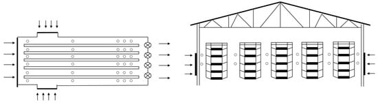
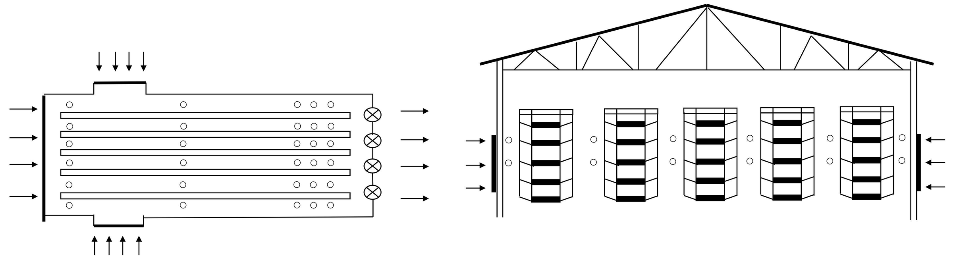
Ten monitoring points were established in each of the six aisles, yielding a total of 60 monitoring locations throughout the facility. Within each aisle, five points were positioned transversely across the width, with each transverse location comprising two vertically stacked sensors—one at the first tier and one at the second tier. The spatial configuration of all monitoring points is illustrated in Figure 1.
Figure 1.
Layout of Measurement Points. ○ indicates the monitoring points, → indicates the direction of the ventilation airflow, from the evaporative cooling pads at the inlet (north wall) to the exhaust fans at the outlet (south wall); ⊗ indicates the exhaust fans.
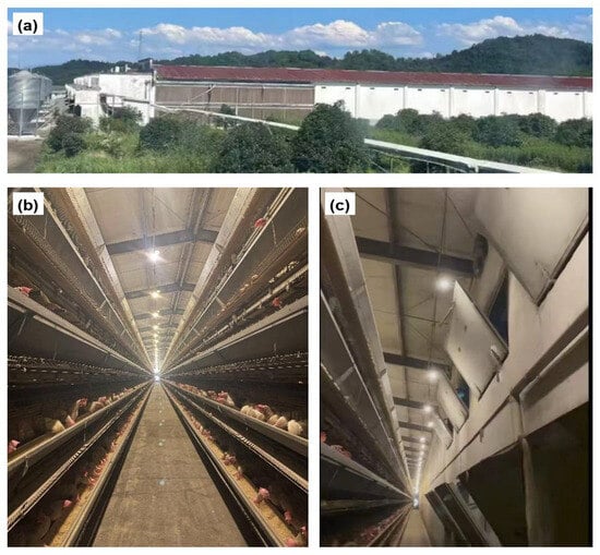
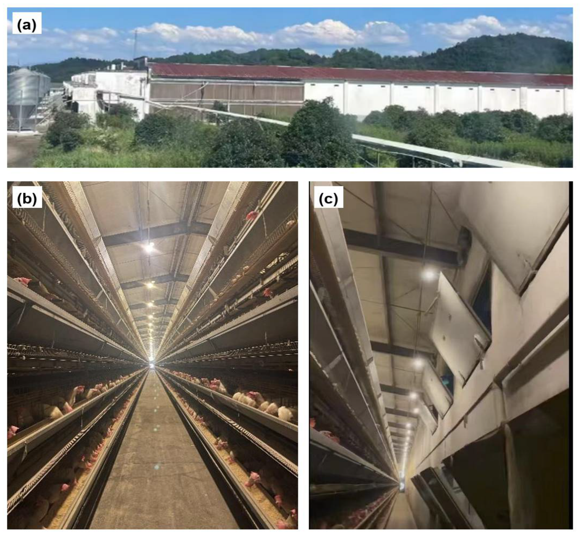
The overall appearance, internal structure, and ventilation openings of the laying hen house are illustrated in Figure 2a–c.
Figure 2.
Overall exterior view and the interior view of the laying hen house. (a) overall exterior view of the laying hen house; (b) internal structure of the laying hen house; (c) ventilation openings of the laying hen house.
The experimental laying hen house measures 90 m in length, 15 m in width, and 7.5 m in height, with a painted steel sheet roof oriented along a north–south axis. The facility employs a longitudinal ventilation system: the north wall functions as the air inlet equipped with evaporative cooling pads, while the south wall serves as the exhaust end housing the fans. The east and west walls are symmetrically configured with equal-area evaporative cooling pads and an identical number of ventilation windows and wind baffles. Internally, the house utilizes a five-tier, five-row stacked cage system without bedding, comprising five rows of double-sided cages with five tiers per side. Furthermore, the facility is equipped with comprehensive automated husbandry systems, including automatic feeding, nipple drinking, conveyor-belt manure removal, and egg collection.
2.2. Data Collection
Data collection was conducted during the summer season, spanning from 1 July to 8 September 2024. Environmental measurements were recorded at 30 min intervals during three daily periods (06:00–08:00, 12:00–14:00, and 18:00–20:00), with values averaged within each period to determine key environmental parameters. Missing values arising from sensor or communication failures were addressed via linear interpolation. These parameters included indoor temperature, relative humidity, and concentrations of critical gases within each poultry house section, as well as outdoor temperature and humidity.
This study employed the ST-BYX four-in-one sensor (Guangzhou Saitong Technology Co., Ltd., Guangzhou, China) to monitor temperature, relative humidity, and CO2 concentration, and the JXBS-3001-PM2.5 RS-485 air quality sensor (Shanghai Bidas IoT Technology Co., Ltd., Shanghai, China) to measure PM2.5 concentration. All sensors were factory-calibrated and integrated into an MCGS configuration monitoring system via the RS-485 communication protocol. The detailed technical specifications of the sensors are presented in Table 1.
Table 1.
Parameters of the sensor.
3. A Multi-Environmental Factor Prediction Model Based on AKF-Attention-CNN-LSTM
3.1. A Model Framework Based on AKF-Attention-CNN-LSTM
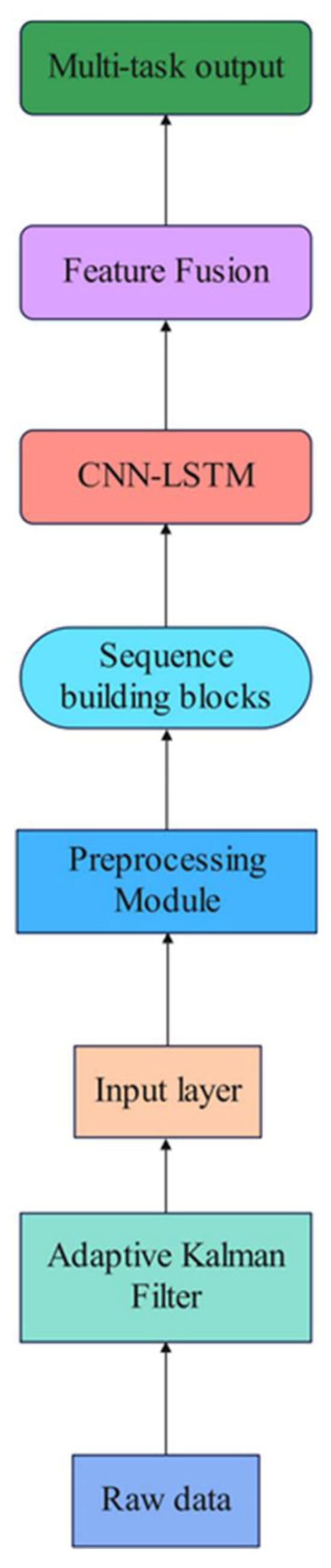
The overall framework of the proposed AKF-Attention-CNN-LSTM model is illustrated in Figure 3. It consists of four sequential stages: adaptive Kalman filtering of the raw sensor data, feature engineering, CNN-based local feature extraction, and LSTM-based temporal modelling followed by the attention mechanism and the output layer.
Figure 3.
Framework of an environmental prediction model for laying hen houses based on AKF-Attention-CNN-LSTM.
Adaptive Kalman Filtering (AKF): Distinct adaptive Kalman filters were configured for each of the four environmental parameters—temperature, relative humidity, carbon dioxide (CO2), and particulate matter (PM2.5). An adaptive noise adjustment mechanism, leveraging the volatility of recent observations, was implemented to dynamically optimize the process noise covariance matrix. A first-order random walk model was employed to simplify the state transition equations and minimize computational overhead.
Input Layer: This layer accepts the denoised time series outputs from the adaptive Kalman filtering stage.
Preprocessing Module: This module performs feature engineering on the Kalman-filtered time series, incorporating three key transformations: (1) first-order differencing to capture temporal trends, (2) moving average smoothing to attenuate short-term fluctuations, and (3) z-score normalization to standardize feature scales. All features undergo z-score normalization prior to network input to mitigate the influence of dimensional heterogeneity among environmental parameters on model convergence and training stability.
Sequence Construction and Dynamic Attention Module: Time-series samples were constructed using a 24 h sliding window to forecast temperature, relative humidity, carbon dioxide (CO2) concentration, and particulate matter (PM2.5) concentration at the subsequent time step. To enhance feature representation at critical temporal positions, a dynamic attention mechanism leveraging the rate of change in environmental parameters was developed. The implementation procedure comprises the following sequential operations:
- Compute the first-order differences in environmental parameter sequences within the sliding window to derive a sequence of change rate values;
- Apply absolute value transformation to the change rate sequence, followed by softmax normalization to generate an attention weight vector;
- Perform element-wise multiplication between the window data and attention weights to produce a weighted feature sequence, emphasizing temporal positions characterized by substantial environmental parameter variations.
CNN-LSTM Hybrid Architecture: The proposed architecture integrates four primary components: one-dimensional convolutional neural networks (1D-CNNs), bidirectional long short-term memory networks (BiLSTMs), unidirectional long short-term memory networks (UniLSTMs), and dropout regularization layers.
Convolutional Neural Network (CNN) Component: The CNN employs 1D convolutional layers with a kernel size of three and 32 filters, utilizing ‘same’ padding to preserve spatial dimensions and extract local temporal pattern features. The rectified linear unit (ReLU) activation function is applied to introduce nonlinearity and enhance the model’s representational capacity.
Bidirectional LSTM Component: The bidirectional LSTM layer is configured with 256 hidden units and operates in sequence-to-sequence mode to simultaneously capture forward and backward temporal dependencies within the input sequences.
Unidirectional LSTM Component: The unidirectional LSTM layer comprises 96 hidden units and utilizes sequence-to-one output mode to concentrate on feature representations at the terminal time step.
Dropout Regularization: A dropout layer with a dropout rate of 0.3 is implemented to randomly deactivate 30% of neurons during training, thereby mitigating overfitting and improving model generalization.
Feature Fusion Module: The feature fusion stage incorporates a sequential processing pipeline comprising a fully connected layer, batch normalization layer, dropout regularization, and a final fully connected layer for output generation.
Fully Connected Layer (128 Neurons): This layer integrates high-level features extracted from preceding layers and learns complex nonlinear mapping relationships between input representations and target outputs.
Batch Normalization Layer: This layer standardizes the inputs to subsequent layers by normalizing the activations, thereby accelerating training convergence and enhancing model stability during optimization.
ReLU Activation Function: The rectified linear unit (ReLU) activation function introduces nonlinearity into the network architecture, enabling the model to learn complex patterns and relationships within the data.
Dropout Layer (Dropout Rate = 0.3): This regularization layer randomly deactivates 30% of neurons during each training iteration to prevent overfitting and improve the model’s generalization capability.
Regression Layer: The output layer employs the mean squared error (MSE) loss function for regression tasks, quantifying the discrepancy between predicted and actual values to guide parameter optimization.
Multi-Task Learning Framework: The proposed architecture implements a multi-task learning approach where a single unified model simultaneously predicts multiple environmental parameters while leveraging shared feature representations across tasks, thereby improving overall predictive performance and computational efficiency.
3.2. Adaptive Kalman Filter
Environmental parameter sensors deployed in poultry housing systems are susceptible to noise interference from complex electromagnetic disturbances and power supply fluctuations generated by high-power ventilation equipment and automated feeding systems during operation. To address this challenge, this study implements an AKF algorithm for preprocessing raw sensor data of multiple environmental parameters. This approach effectively suppresses both system noise and environmental interference, minimizes random measurement errors, and facilitates temporal data fusion. The preprocessing pipeline comprises two sequential stages: (1) data quality assurance, wherein missing sensor readings resulting from collection anomalies are imputed using linear interpolation, and statistical outliers are identified and removed; and (2) adaptive filtering, wherein the AKF algorithm smooths the preprocessed time series by eliminating abrupt fluctuations and correcting measurement deviations, thereby ensuring data accuracy and validity for subsequent analysis.
Conventional Kalman filtering methodologies presuppose that the process noise covariance matrix (Q) and measurement noise covariance matrix (R) remain known and invariant throughout operation. However, in practical implementations, noise characteristics frequently exhibit temporal variations correlated with environmental dynamics, resulting in diminished filtering efficacy. Adaptive Kalman filtering addresses this limitation by incorporating a dynamic parameter adjustment mechanism that extends conventional Kalman filtering principles, enabling real-time adaptation of filter parameters in response to evolving system states and fluctuating noise properties. This enhancement introduces an adaptive update procedure integrated within the standard Kalman filtering framework:
Calculate the residuals:
Adaptively update the noise matrix and compute using a sliding window
Compute the Kalman gain and recalculate the Kalman gain Kk using the updated :
Status update:
Pk|k = (I − KkHk) Pk|k−1
Here, Zk is the actual observation, Hk is the observation matrix, xk is the prior state estimate, is the estimated measurement noise covariance, N is the sliding window size, and Pk is the posterior estimated covariance, which represents the degree of uncertainty regarding the “final result” and is used as the initial value for the next time step.
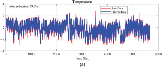
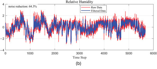
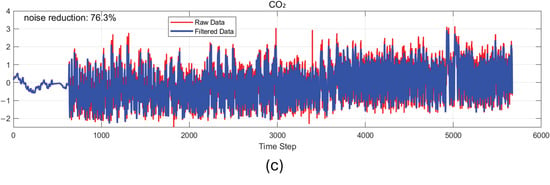
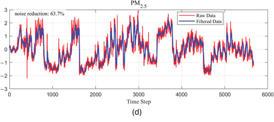
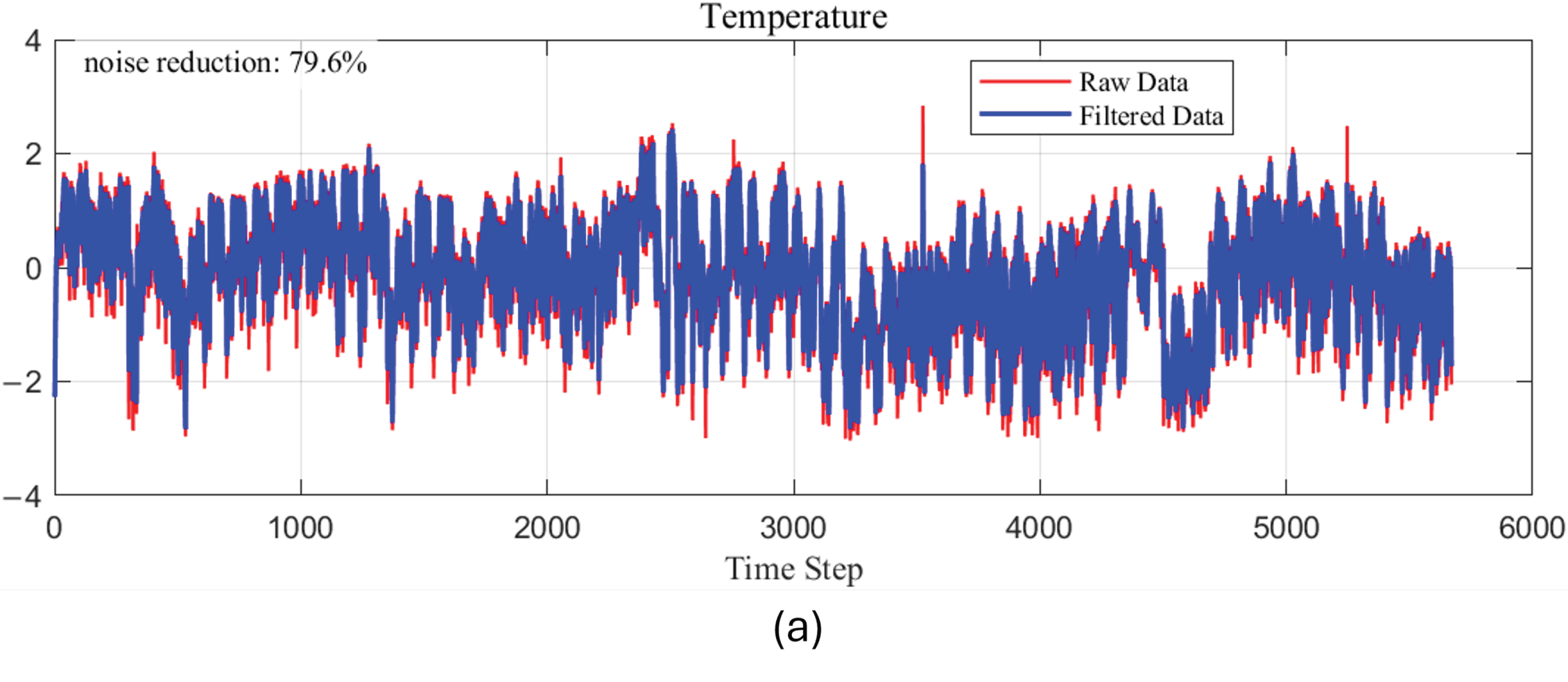
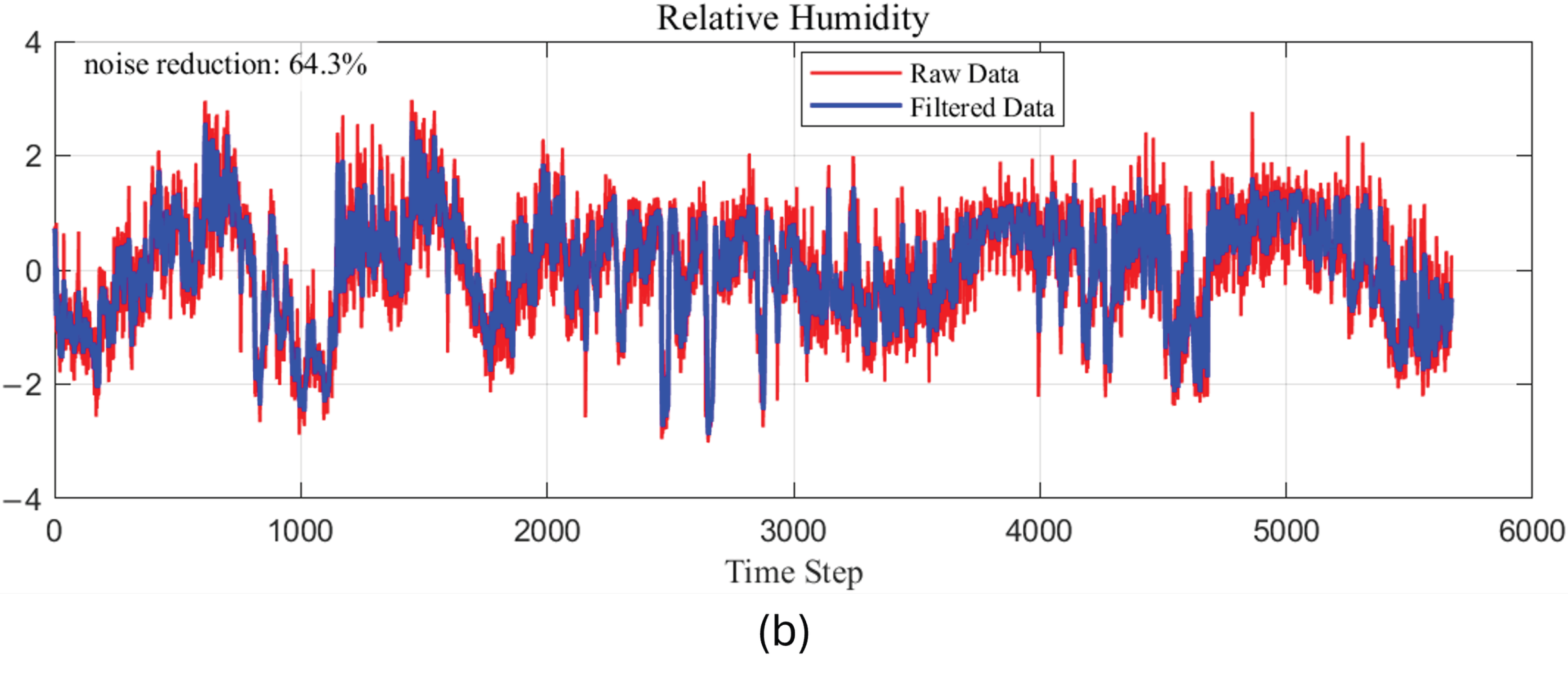
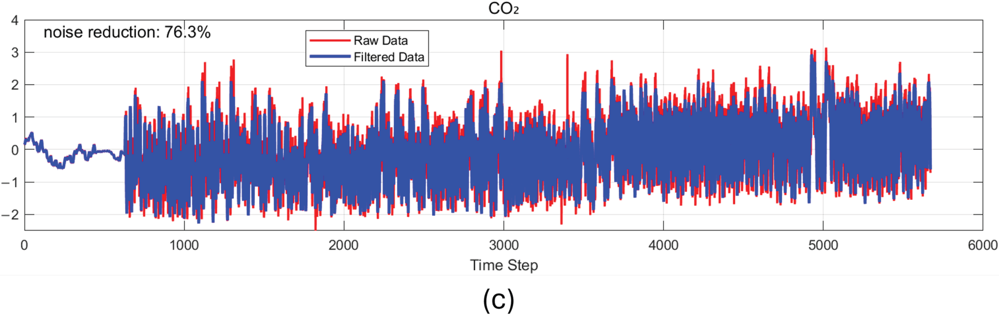
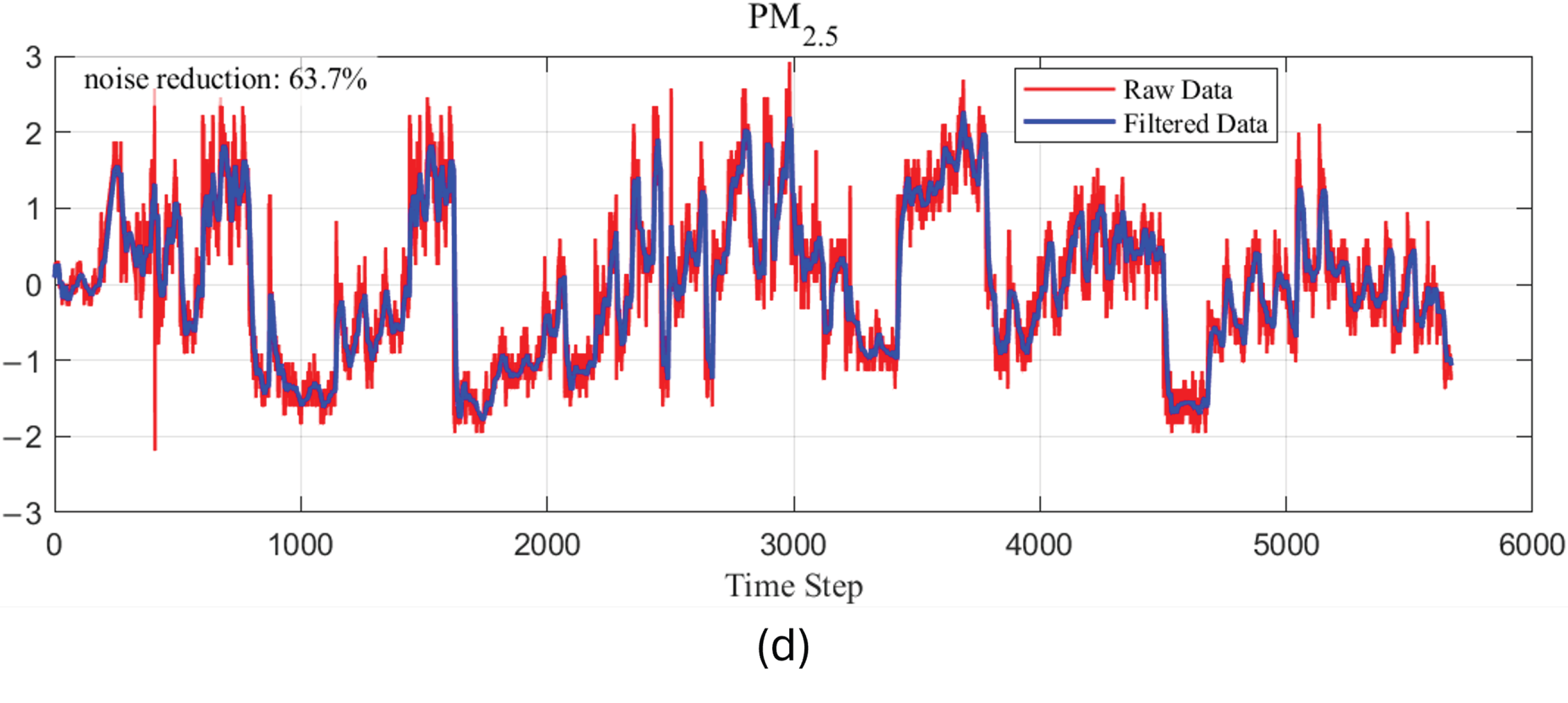
Figure 4 illustrates the environmental data processed using the adaptive Kalman filter (AKF) algorithm. The temperature data filtering achieved a noise suppression rate of 79.6%, effectively attenuating high-frequency measurement noise while preserving diurnal periodic variation characteristics. The standard deviations of temperature measurements decreased from 1.000 °C to 0.939 °C following filtering, with complete retention (100%) of abrupt changes. Relative humidity filtering yielded a noise reduction rate of 64.3%, with standard deviations decreasing from 1.000% to 0.895% and perfect retention (100%) of sudden variations. Carbon dioxide (CO2) concentration filtering demonstrated a noise reduction rate of 76.3%, with standard deviations declining from 1.000 ppm to 0.515 ppm while maintaining 100% retention of abrupt changes. Particulate matter (PM2.5) filtering achieved a noise reduction rate of 63.7%, with standard deviations decreasing from 1.000 μg/m3 to 0.925 μg/m3 and a 95.9% retention rate for sudden changes. These results demonstrate that the adaptive Kalman filter effectively mitigates measurement noise across diverse environmental parameters, reduces data fluctuations, enhances the signal-to-noise ratio, and improves data validity, thereby providing high-quality input data for subsequent deep learning modeling.
Figure 4.
(a) Comparison of Raw Temperature Data with Kalman Filter Results; (b) Comparison of Raw Relative Humidity Data and Kalman Filter Results; (c) Comparison of Raw CO2 Data and Kalman Filter Results; (d) Comparison of Raw PM2.5 Data and Kalman Filter Results.
3.3. Convolutional Neural Networks and Long Short-Term Memory Networks
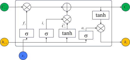
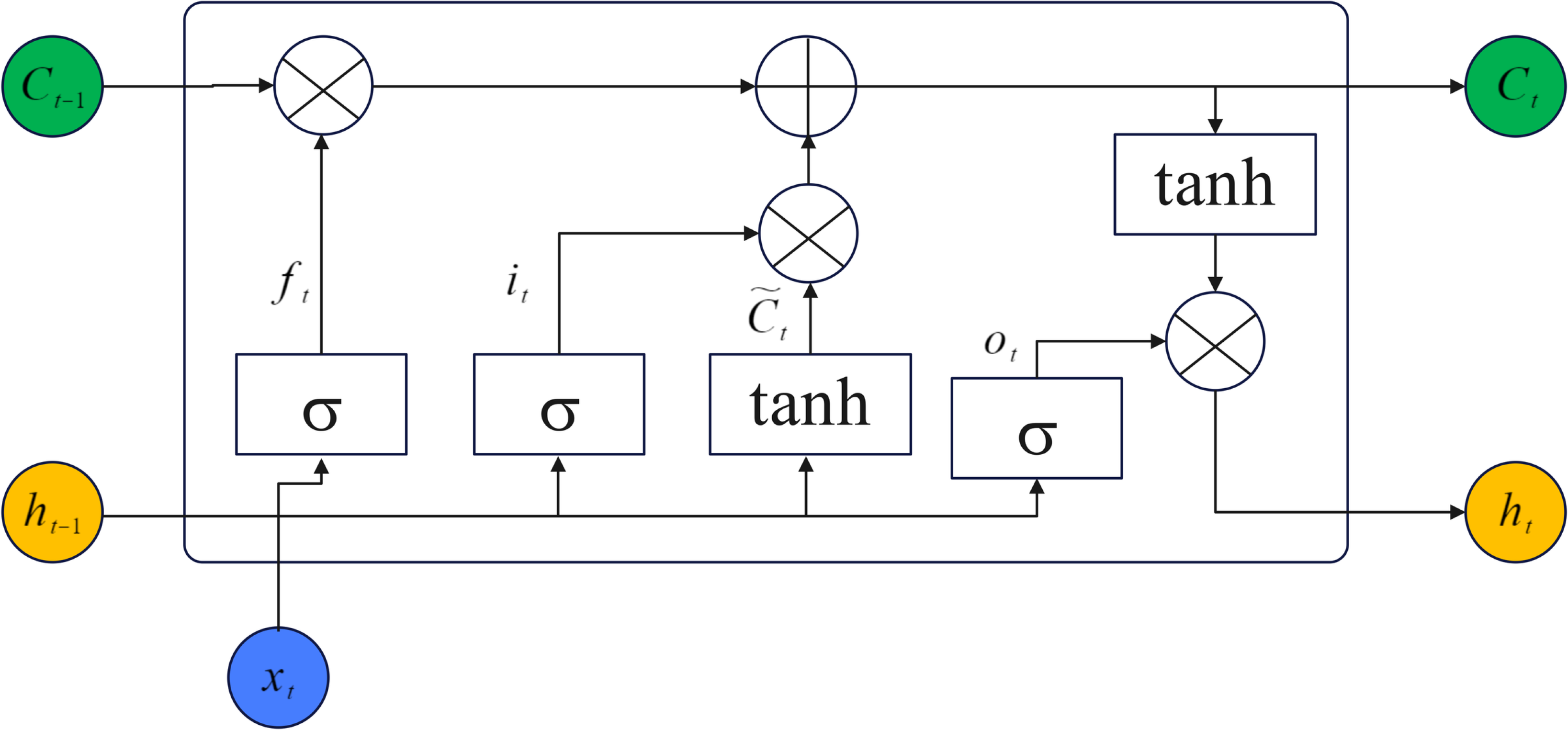
The Long Short-Term Memory (LSTM) network constitutes a specialized recurrent neural network (RNN) architecture engineered for modeling and forecasting sequential data. Its gating mechanism effectively resolves the long-term dependency problem inherent in conventional RNNs. Specifically, LSTM networks mitigate vanishing and exploding gradient phenomena prevalent in extended sequences, thereby enabling robust capture of contextual information across temporal spans. Complementarily, Convolutional Neural Networks (CNNs) extract short-term temporal patterns from localized windows through convolutional operations. The hybrid CNN-LSTM architecture introduced in this study first employs CNNs to discern local temporal features; these features are subsequently processed by a hierarchical configuration of bidirectional and unidirectional LSTM layers to capture multi-scale temporal dependencies. This integrated framework facilitates high-accuracy prediction of environmental parameters using exclusively historical time-series data. Figure 5 illustrates the LSTM cell architecture.
Figure 5.
Schematic diagram of an LSTM cell structure. σ A fully connected layer with an activation function; ⨂ denotes element-wise multiplication, and ⨁ denotes element-wise addition.
The Long Short-Term Memory (LSTM) network extends the recurrent neural network (RNN) architecture by incorporating a memory cell and three gating mechanisms that regulate information flow: the input gate, forget gate, and output gate. The forget gate determines the proportion of historical memory to retain, producing an output denoted as ft; the input gate governs the extent of new information to integrate, yielding an output it; and the output gate modulates the fraction of internal memory state to propagate as the current output, generating ot. The hyperbolic tangent (tanh) activation function introduces nonlinearity and compresses the numerical range to [−1, 1], thereby mitigating gradient explosion and enhancing training stability.
Compute the three gate signals based on the current input Xt and the previous hidden state ht−1
ft = σ (Wf∙[xt;ht−1] + bf)
it = σ (Wi∙[xt;ht−1] + bi)
ot = σ (Wo∙[xt;ht−1] + bo)
In particular, [xt;ht−1] denotes concatenating the input vector with the previous hidden state to form a long vector, where Wf, Wi, Wo are learnable weight matrices; and bf, bi and bo are bias terms.
Calculate the candidate cell state
tanh compresses the values into the range (−1, 1), serving as latent new memories.
Update cell state
ft⊙Ct−1 Selective forgetting of old memories, selectively writes new information.
Compute the current hidden state ht:
ht = ot⊙tanh (Ct)
This study employs time-series data refined by an adaptive Kalman filter as input to a hybrid CNN-LSTM architecture, establishing a framework for the collaborative forecasting of multiple environmental parameters in laying hen houses that integrates robustness to data quality with high predictive accuracy.
4. Results and Discussion
4.1. Parameter Settings
As shown in Table 2, the noise parameters for CO2 and PM2.5 are relatively large, indicating significant fluctuations in actual measurements; the parameters for temperature and relative humidity are relatively small, indicating relatively stable variations. The adaptive mechanism of AKF works as follows: when data fluctuates significantly, it automatically increases the process noise Q, causing the filter to place greater trust in the current observed values; when data is stable, it reduces Q, causing the filter to rely more on the predicted values. The range of the Kalman gain K is [0, 1]. When K→1, the filter places greater trust in the observed values (i.e., the observation noise R is small); when K→0, the filter places greater trust in the predicted values (i.e., the process noise Q is relatively small).
Table 2.
Noise Settings in AKF.
Table 3 presents the hyperparameter configuration for the hybrid CNN-LSTM architecture employed in this research. The Adam optimization algorithm was selected to facilitate adaptive learning rate adjustment. The training regimen comprised 80 epochs with a batch size of 64 samples per iteration. An initial learning rate of 0.001 was implemented, coupled with a stepwise decay strategy that reduced the learning rate by half every 20 epochs. To mitigate overfitting, early stopping was configured with a patience parameter of 8 epochs, terminating training upon failure to improve validation performance for eight consecutive epochs. Additionally, gradient clipping was activated with a threshold of 1.0 to constrain gradient magnitudes and prevent numerical instability. This comprehensive hyperparameter configuration ensures training stability while optimizing the trade-off between convergence velocity and model generalization capacity.
Table 3.
Hyperparameter Settings for CNN-LSTM.
4.2. Model Evaluation
4.2.1. Experimental Parameters
To ensure the reliability and reproducibility of experimental results, all model training and performance evaluations in this study were conducted under a unified experimental environment, as detailed in Table 4.
Table 4.
Experimental Environment Configuration.
4.2.2. Dataset
This research employed environmental monitoring data collected from a laying hen house. The dataset encompassed four key environmental parameters: temperature, relative humidity, CO2 concentration, and PM2.5 concentration. Feature engineering was implemented to construct an augmented dataset comprising raw measurements, first-order difference features, and moving average features.
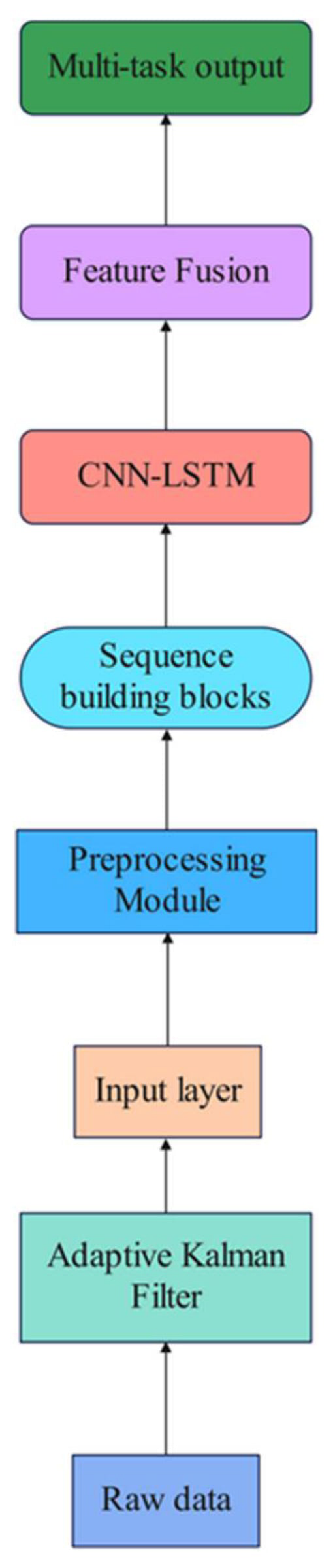
The proposed feature engineering framework, illustrated in Figure 6, encompasses four core modules: basic feature extraction, time-series derivative feature construction, smoothed trend feature generation, and dynamic attention weighting. Through multi-dimensional feature integration, this framework enhances the model’s capacity to capture nonlinear patterns in environmental parameters.
Figure 6.
Feature Engineering Framework Diagram.
- Basic Feature Extraction
Let the original time series be , where xt ∈ R2 represents the temperature observation at time t. First, extract the basic features:
Here, Tempt represents the normalized temperature value, which is standardized using the Z-score:
- 2.
- Construction of Time-Series Derivative Features
To capture instantaneous variations in environmental parameters, first-order difference features are introduced to quantify changes between consecutive time steps:
∆Tempt = Tempt − Tempt−1
This feature effectively identifies abrupt changes and trend reversals, thereby enhancing the model’s sensitivity to sharp fluctuations in environmental parameters.
- 3.
- Generation of Smoothed Trend Features
To mitigate measurement noise and extract long-term temporal trends, a causal moving average (CMA) is employed for signal smoothing:
where the window size w = 3 represents the average of the past three time steps.
- 4.
- First-Order Derivative Features
The instantaneous rate of change of environmental parameters is further computed to capture their acceleration characteristics:
This feature quantifies the acceleration or deceleration process of environmental parameters, providing the foundation for dynamic weight assignment in the attention mechanism.
- 5.
- Feature Enhancement and Concatenation
The aforementioned features are concatenated to construct an enhanced feature vector for subsequent model input.
Xaug = [Xbase, ∆X, XMA, X′]
The dataset was partitioned into training, validation, and test subsets using a 7:1.5:1.5 ratio and subsequently normalized via Z-score standardization. Carbon dioxide concentrations were subjected to logarithmic transformation to address scale disparities among variables. A 24 h sliding window approach was adopted to generate time-series samples for forecasting the four environmental parameters at subsequent time intervals. Model performance was rigorously assessed using three evaluation metrics: Root Mean Square Error (RMSE), Mean Absolute Error (MAE), and the Coefficient of Determination (R2).
Prior to sliding window generation, the dataset was chronologically partitioned into training, validation, and test sets in a 7:1.5:1.5 ratio. Each window was assigned exclusively to a single subset and was constrained not to span subset boundaries, thereby ensuring no temporal overlap or information leakage between the training and evaluation data.
4.2.3. Evaluation Criteria
This paper employs three evaluation metrics to comprehensively assess the model’s predictive performance: Root Mean Square Error (RMSE), which measures the degree of deviation between predicted and actual values and is more sensitive to large errors; Mean Absolute Error (MAE), which measures the average magnitude of prediction errors and provides an intuitive reflection of prediction accuracy; and the Coefficient of Determination (R2), which measures the model’s ability to explain data variability. The formulas for these three metrics are as follows:
Here, n is the total number of samples, yi is the true observed value of the i-th sample, is the model’s predicted value for the i-th sample, SSres is the sum of squared residuals (reflecting model error), and SStot is the total sum of squares (reflecting the total variance of the data). Smaller values of RMSE and MAE indicate higher prediction accuracy, while an R2 closer to 1 indicates better model fit.
4.3. Analysis of Results
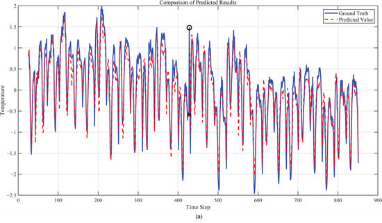
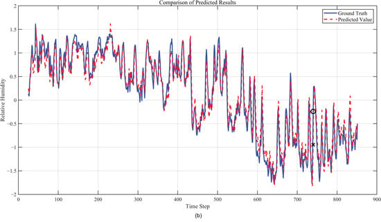
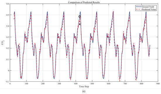
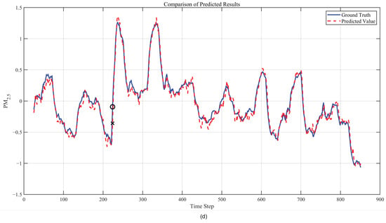
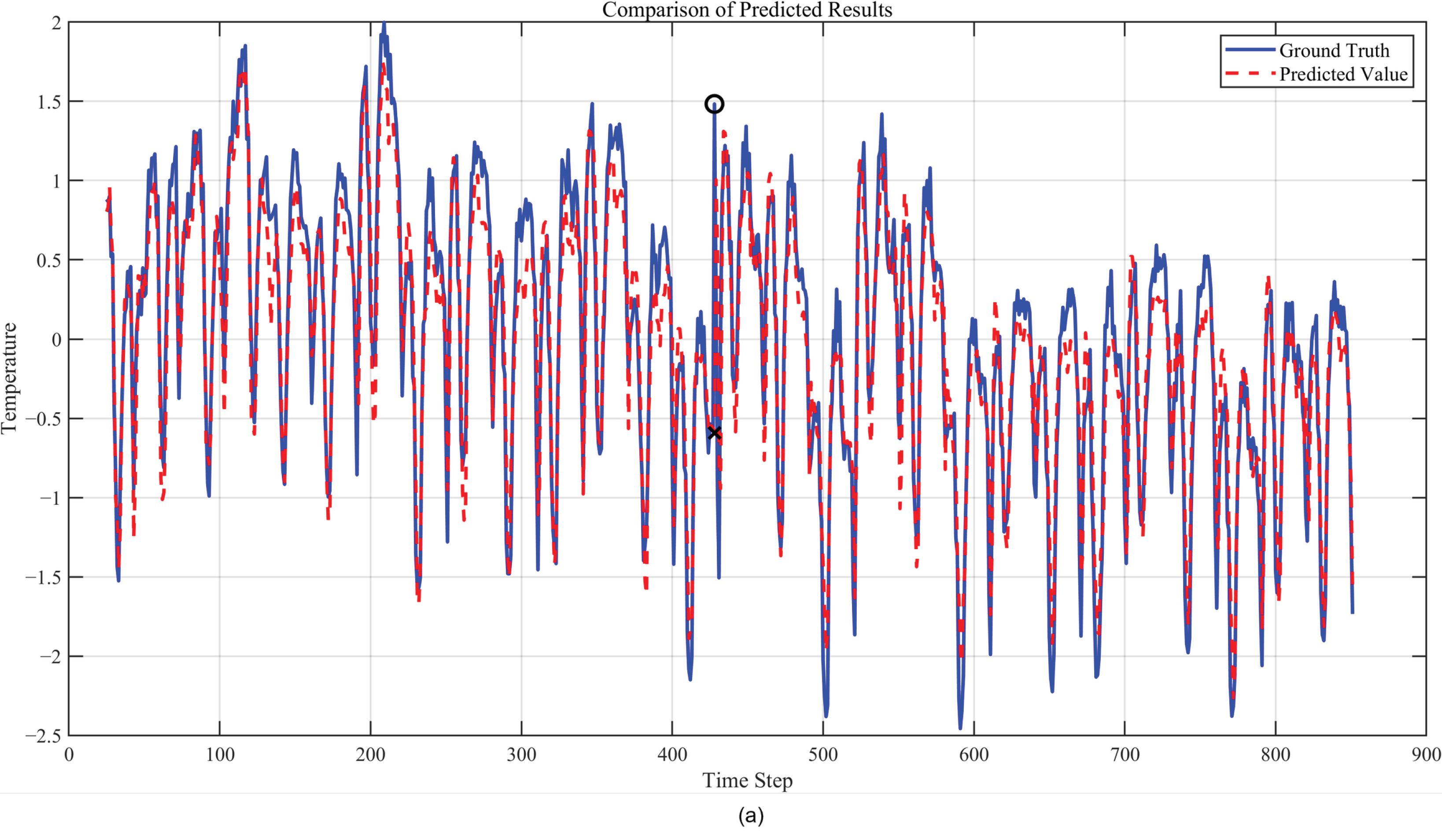
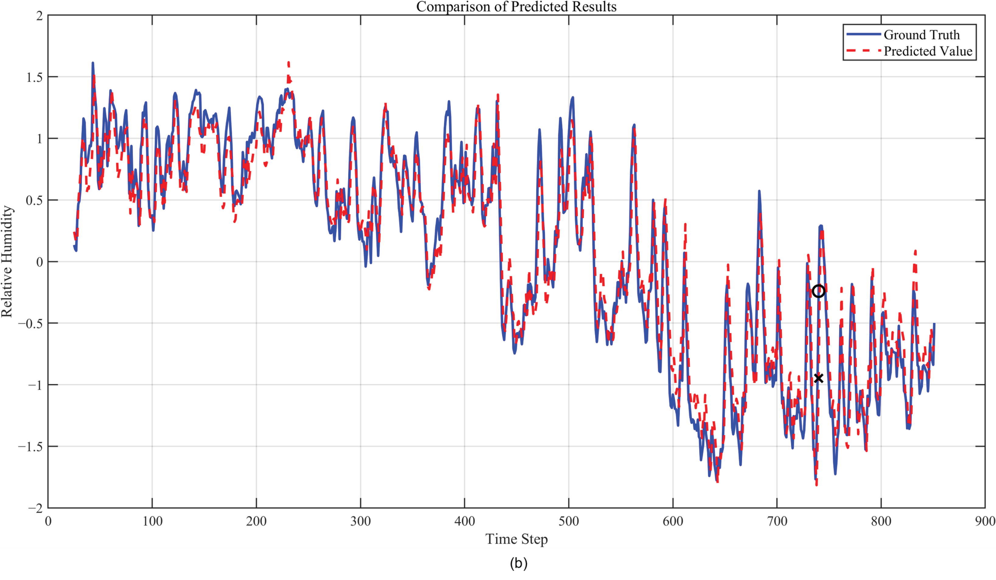
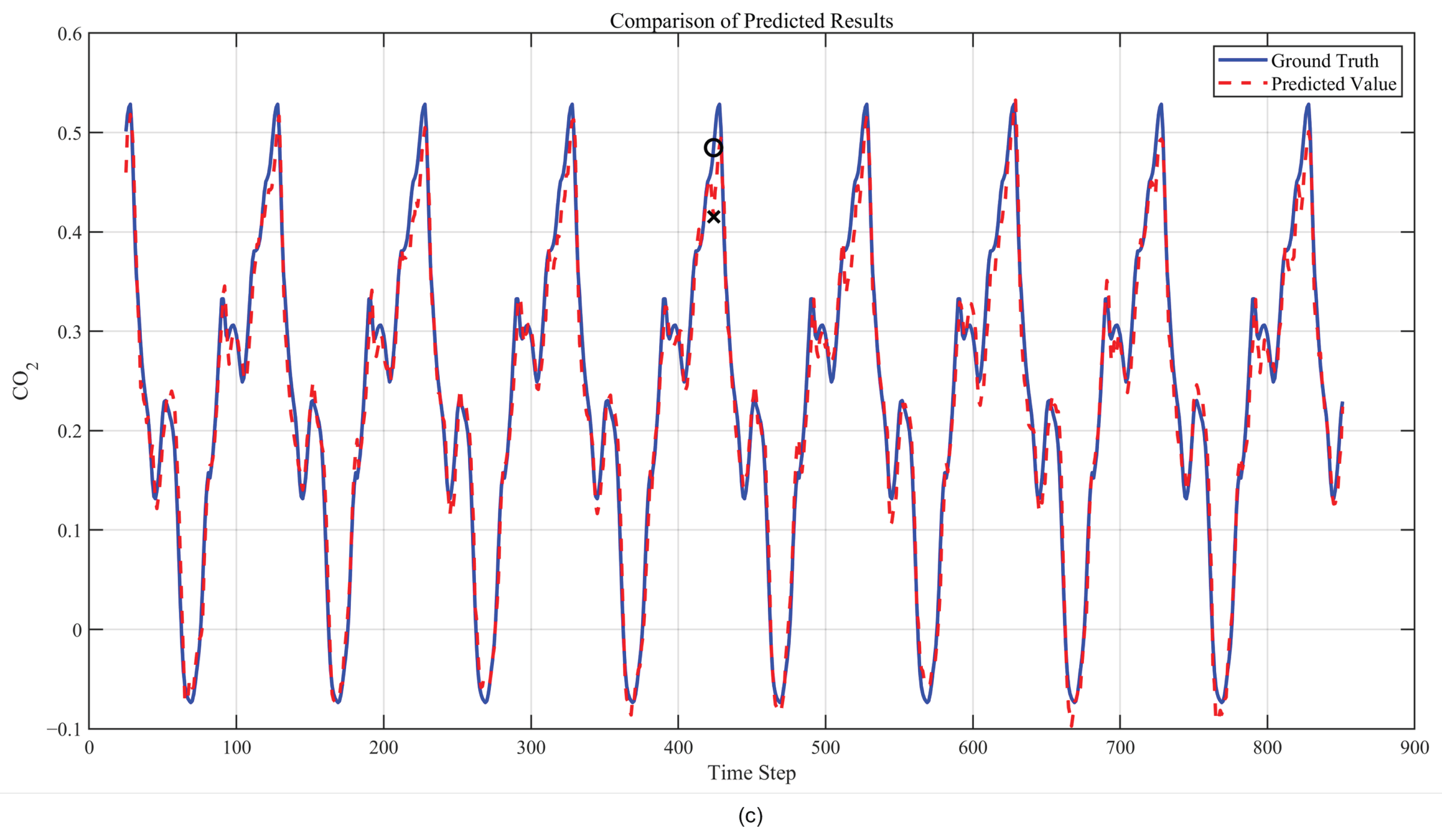
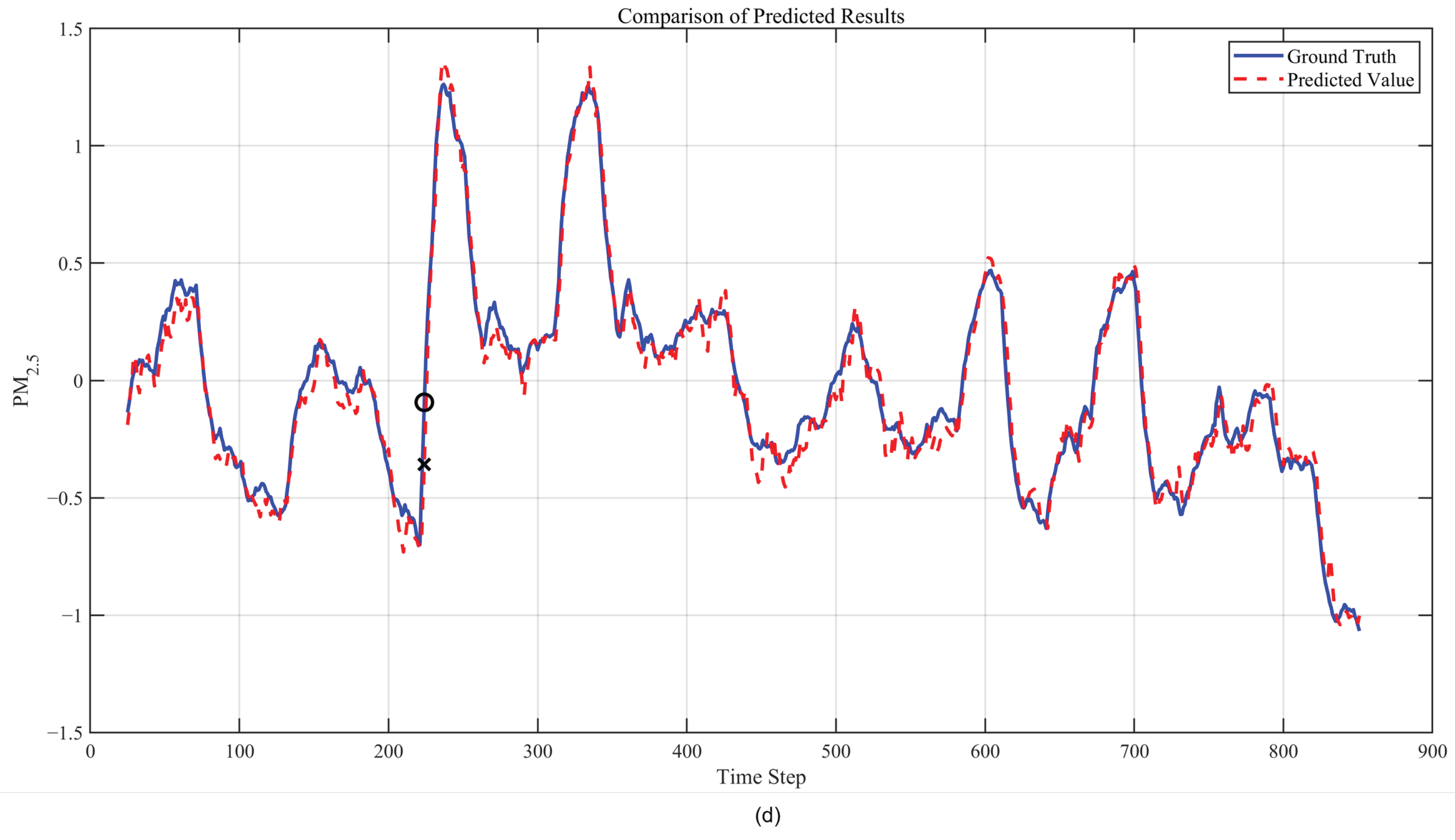
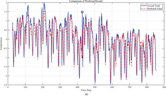
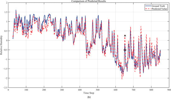
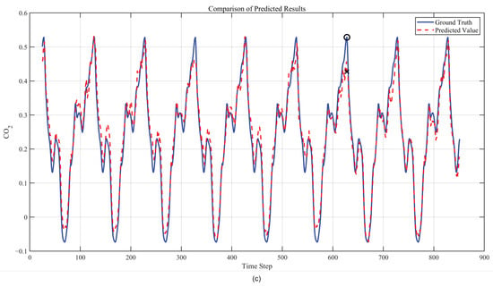
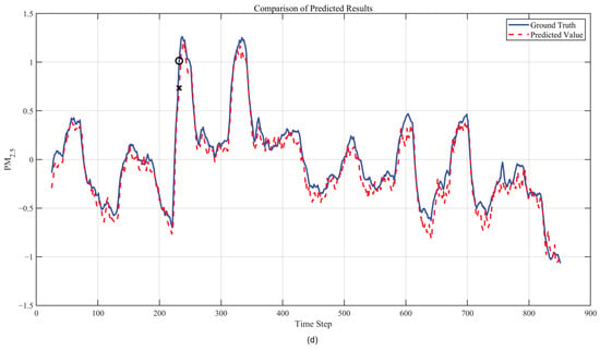
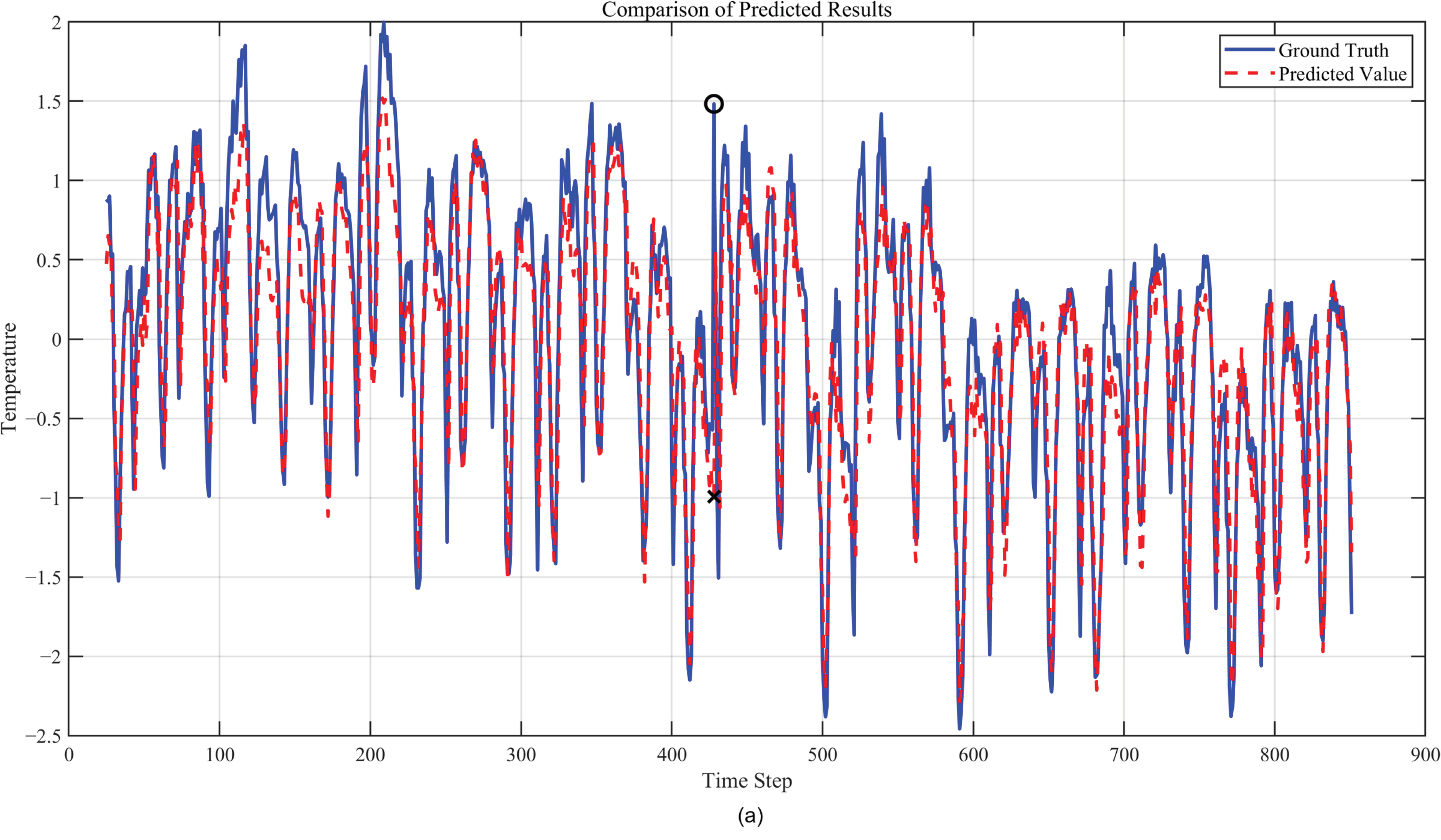
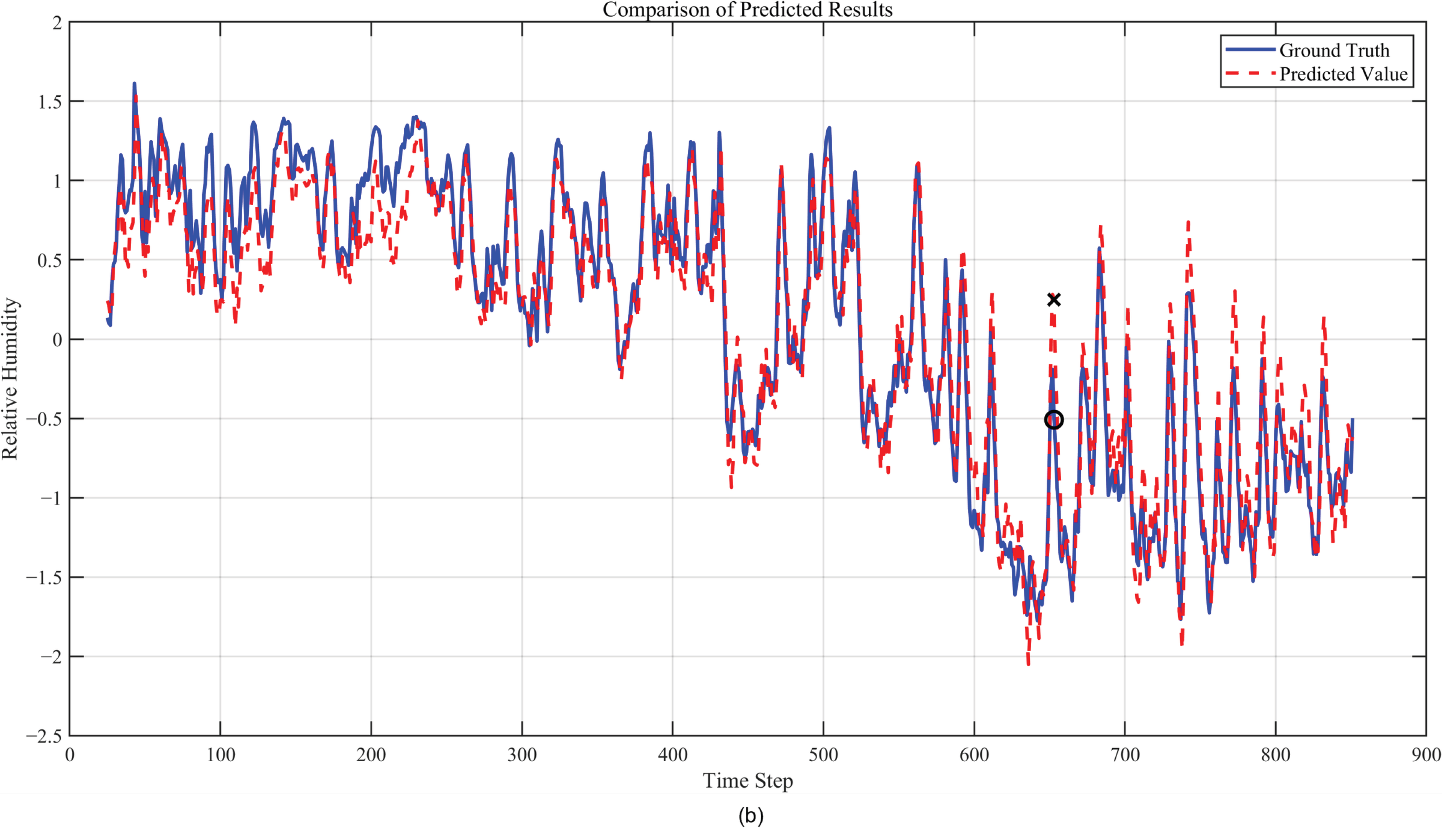
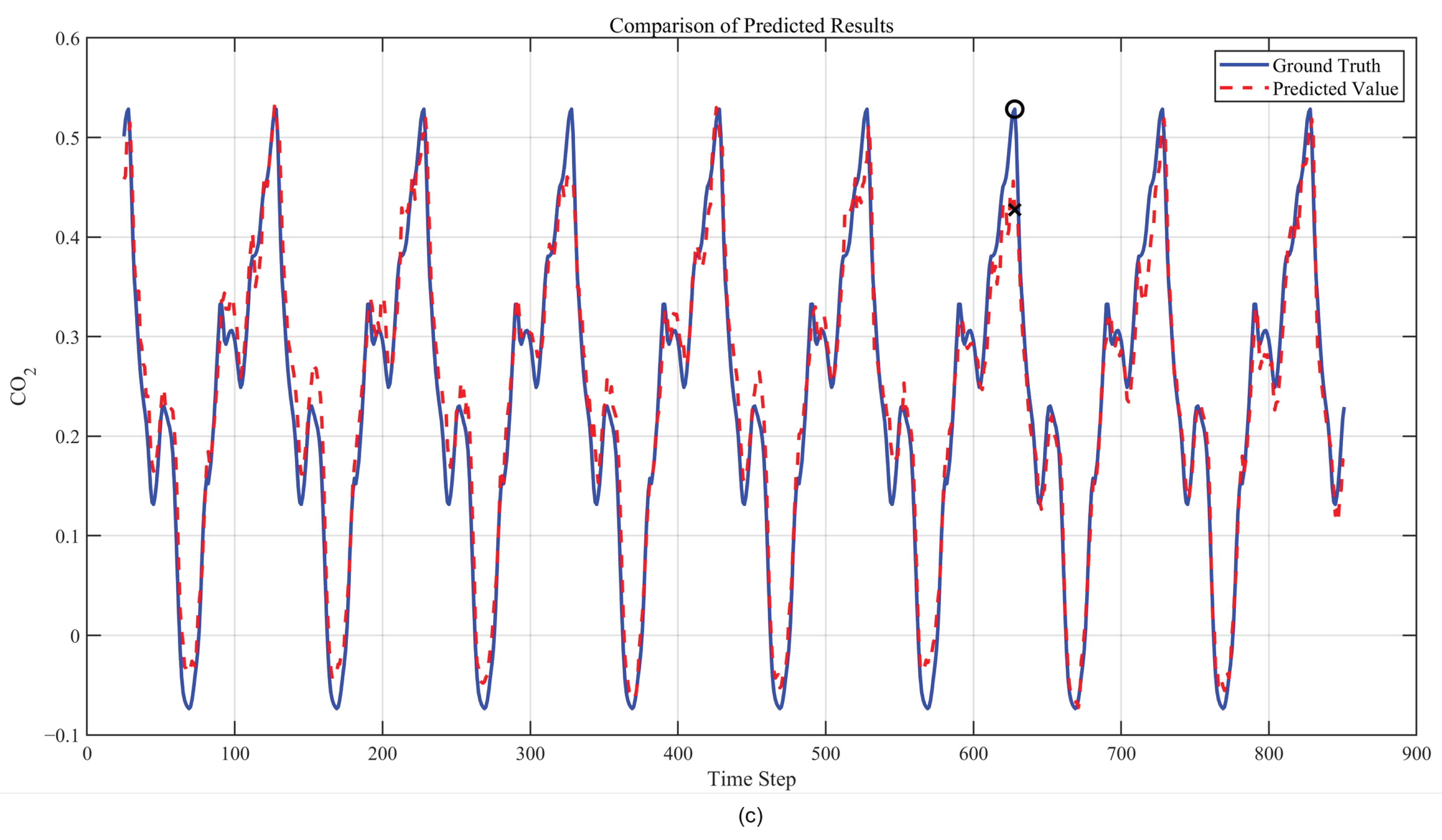
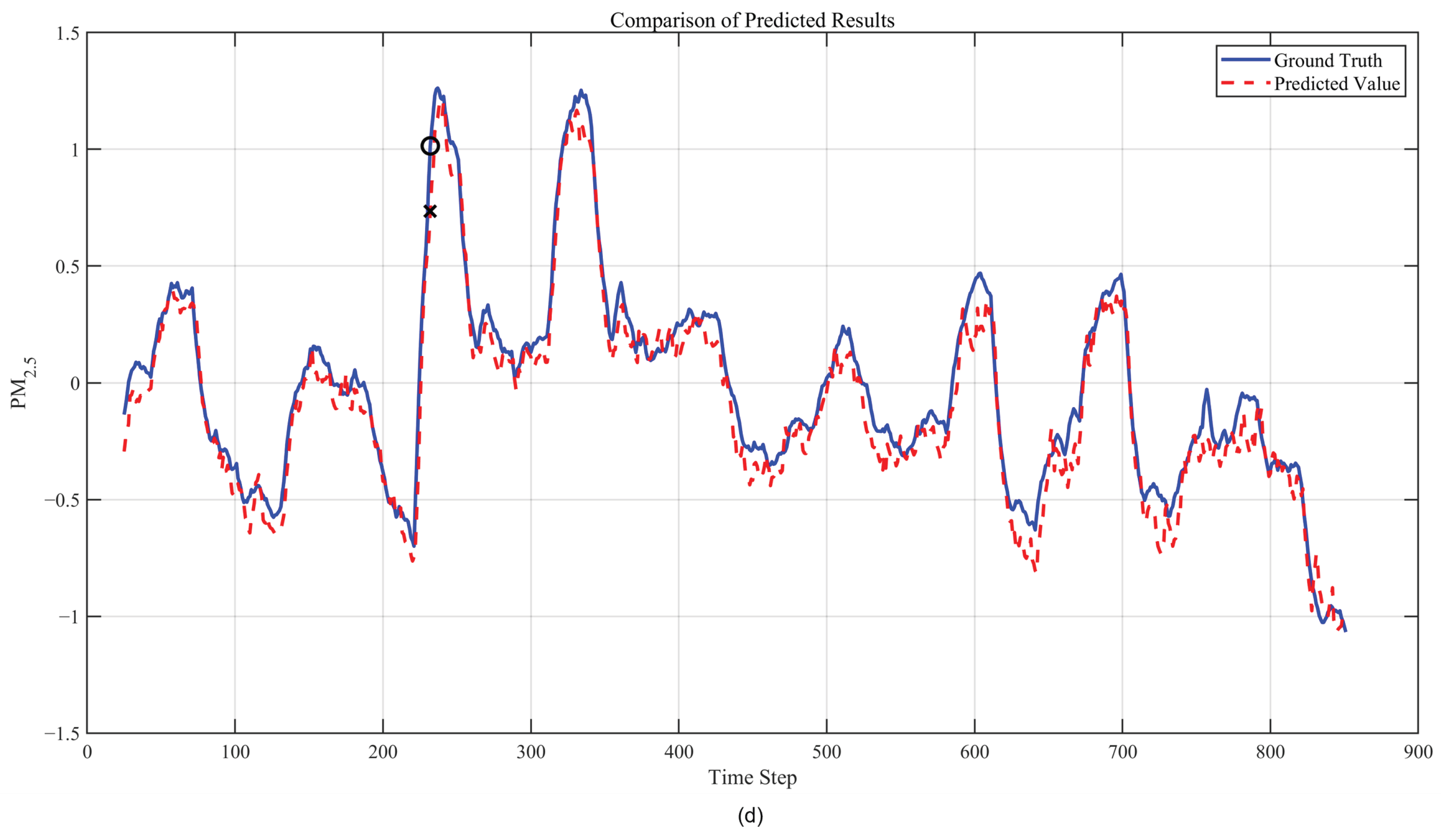
The experimental results are shown in Figure 7.
Figure 7.
Experimental Results: (a) Temperature Prediction Results; (b) Relative Humidity Prediction Results; (c) CO2 Prediction Results; (d) PM2.5 Prediction Results. ○ denotes the maximum error point of the measured values, and × denotes the maximum error point of the predicted values.
Table 5 presents the 5-day monitoring data for monitoring point 1-1-1, the first monitoring point on the upper level of the first passageway. A total of 70 days of data were collected between 1 July and 8 September. For each monitoring point, the measurements at each time interval represent averaged values obtained through interval sampling.
Table 5.
Measured Data from Monitoring Point 1-1-1.
Statistical analyses were performed on all monitored variables over the measurement period. Table 6 summarizes the diurnal (morning, noon, and evening) and monthly variations in these parameters. The mean indoor temperature was 29.8 ± 1.2 °C, which falls within the slightly warm thermal comfort range for laying hens during summer. A pronounced diurnal pattern was observed, with noon temperatures significantly exceeding those recorded in the early morning and evening. The mean relative humidity (RH) was 83.8 ± 6.5%, peaking in the early morning and reaching a minimum at midday; this trend aligns with the operational schedule of evaporative cooling and afternoon ventilation for dehumidification. The mean CO2 concentration was 983.8 ± 119.4 ppm, exhibiting both an evening peak and a progressive monthly increase from July to September, consistent with reduced ventilation rates and gradual CO2 accumulation as ambient temperatures decline. The mean PM2.5 concentration was 30.9 ± 1.8 μg/m3, displaying a relatively high coefficient of variation. PM2.5 levels peaked at midday and showed transient spikes during activities such as feeding and manure removal, indicative of non-stationary behavior. Correlation analysis revealed a strong positive association between temperature and PM2.5, a moderate positive association between temperature and CO2, and a negative association between temperature and RH. These findings confirm the coupled, nonlinear dynamic interactions among environmental factors within the barn.
Table 6.
Statistics on Daily and Monthly Variations.
Based on the comprehensive evaluation metrics, the AKF-Attention-CNN-LSTM model achieved high prediction accuracy across all environmental factors. The corresponding performance metrics for the four environmental factors are summarized in Table 7.
Table 7.
Experimental Results for Four Environmental Factors.
The R2 values for predicting CO2 and PM2.5 concentrations were both higher than 0.97, indicating that the model can explain over 97% of the temporal variation and possesses extremely strong time series fitting capabilities; the R2 values for temperature and relative humidity reached 0.8853 and 0.9519, respectively, demonstrating that the model also exhibits good predictive performance for environmental factors with high volatility. In terms of RMSE and MAE values, the error margins for CO2 and PM2.5 concentrations were controlled between 0.01 and 0.07, with relatively small absolute errors, meeting the practical requirements for prediction accuracy in the precise environmental control of layer houses.
In terms of dynamic tracking, the predicted curves for all parameters closely matched the actual values. The model maintained strong tracking capabilities even during sudden changes in environmental parameters: for example, when temperature showed a rapid downward trend around steps 200 and 550, the predicted curve followed synchronously without significant phase lag or overshoot; CO2 concentration experienced a sudden surge around step 600, and the model accurately captured the peak trend within 1–2 time steps; PM2.5 concentration exhibited a sharp negative pulse around step 230, and the predicted values precisely reproduced this transient characteristic. These results indicate that the model not only learns the steady-state variation patterns of environmental parameters but is also capable of effectively capturing non-stationary abrupt changes triggered by external disturbances, demonstrating its adaptability in real-world farming scenarios.
Moreover, accurately reproducing the aforementioned PM2.5 transient features has significant implications for livestock production. Indoor particulate matter concentrations (predominantly PM2.5) are governed primarily by facility management practices rather than external climatic factors alone. Specifically, ventilation cycling, fan operation, routine tasks (e.g., manure removal, egg collection, feeding, and lighting), cleaning protocols, and seasonal environmental control directly disrupt indoor airflow patterns and dust suspension dynamics, thereby inducing rapid PM2.5 fluctuations. Consequently, PM2.5 time series exhibit non-stationary behavior with frequent abrupt changes that are temporally coupled to management activities.
Therefore, accurate PM2.5 prediction cannot rely solely on smooth temporal extrapolation; models must capture transient pulses induced by operational events. The precise reconstruction of the negative pulse at step 230 in this study demonstrates that, under a one-step-ahead (1 h) framework, the proposed model effectively captures such abrupt, management-driven dynamics. This capability holds considerable engineering value. First, it provides a basis for optimizing the timing of management interventions (e.g., ventilation and manure removal) and for early warning of dust exposure risks. Second, it underscores the necessity of incorporating operational variables (e.g., ventilation status and activity schedules) into indoor environmental prediction models to improve forecasting accuracy for management-dependent parameters such as PM2.5.
In long-term time series forecasting, all environmental factors exhibit distinct periodic fluctuations, which are closely related to daily management operations in the chicken house. Relative humidity exhibits regular fluctuations approximately every 200 steps; the predicted curve is in phase with the actual value curve, with minimal amplitude error. CO2 and PM2.5 concentrations similarly display synchronized periodic peak-trough structures, indicating that the model has successfully encoded the closed-loop dynamic mechanism of operation-environment feedback in the chicken house. This validates the model’s effectiveness in modeling multiscale temporal dependencies.
To evaluate the performance of the proposed model relative to established baselines, comparative experiments were conducted using LSTM and BiLSTM on the test set. The results are summarized in Table 8.
Table 8.
Performance evaluation of different models.
As shown in Table 8, the proposed model significantly outperforms the unidirectional LSTM across all four environmental variables. Compared with the unidirectional LSTM, the proposed model reduces the average RMSE from 0.2122 to 0.1447 (31.8%) and the average MAE from 0.1688 to 0.1114 (34.0%), while increasing the average R2 from 0.8832 to 0.9488 (+6.57 percentage points). The unidirectional LSTM processes sequences exclusively in the forward temporal direction, precluding access to bidirectional contextual information. Moreover, without dedicated denoising or time-frequency feature extraction, it cannot adequately capture abrupt transitions and noise in environmental signals. In contrast, the proposed model integrates an AKF for signal denoising, an attention mechanism for adaptive weighting of critical time steps, and a CNN for local time-frequency feature extraction, thereby yielding consistent performance gains across all four variables.
Although the BiLSTM outperforms the unidirectional LSTM via bidirectional modeling, its overall performance remains inferior to that of the proposed model. Compared with the BiLSTM, the proposed model reduces the average RMSE and MAE by 22.6% and 23.7%, respectively, while increasing the average R2 by 3.76 percentage points. Notably, the performance gains of the proposed model exhibit a gradient pattern across different variables. The improvements are most pronounced for temperature—a variable subject to equipment control and high stochasticity—yielding a 27.3% reduction in RMSE and a 10.27 percentage point increase in R2. Conversely, for CO2, which exhibits the strongest periodicity, the improvements are relatively modest, with a 17.7% reduction in RMSE and a 0.92% increase in R2; nevertheless, its R2 reaches 0.9815, approaching the theoretical upper limit. This phenomenon indicates that while the bidirectional structure of the BiLSTM effectively captures the temporal dependencies of highly periodic variables, the additional gains of the proposed model primarily stem from the AKF-based filtering of non-stationary, highly transient signals and the CNN-based extraction of local features. These mechanisms effectively compensate for the inherent limitations of recurrent neural networks in processing such complex signals.
Overall, the multi-environmental factor prediction model based on AKF-Attention-CNN-LSTM demonstrates excellent performance in terms of absolute error, trend fitting capability, and sudden change tracking. It effectively models the nonlinear dynamic characteristics and long-term and short-term dependencies of environmental parameters in layer houses, making it suitable for real-time monitoring and feedforward control scenarios in layer house environments. This model provides reliable predictive support for the engineering implementation of intelligent environmental control systems.
To demonstrate the contribution of the proposed Attention mechanism to the model’s predictive performance, this study designed ablation experiments: while keeping the CNN-LSTM network architecture and hyperparameters completely consistent, the dynamic Attention module was removed to compare the differences in predictive performance between the full model and the ablated model across four environmental factors.
4.4. Ablation Experiment
Quantitative analysis of the ablation experiment results shows that the full model outperforms the ablated model on all evaluation metrics, as illustrated in Figure 8.
Figure 8.
Ablation experiment results: (a) Temperature prediction results from ablation study; (b) Relative humidity prediction results from ablation study; (c) CO2 prediction results from ablation study; (d) PM2.5 prediction results from ablation study. ○ denotes the maximum error point of the measured values, and × denotes the maximum error point of the predicted values.
Table 9 compares the ablation experiment results for the four environmental factors.
Table 9.
Ablation Experiment Results for Four Environmental Factors.
Temperature: R2 increased from 0.8363 to 0.8853 (a 5.9% improvement), and RMSE decreased from 0.3537 to 0.2962 (a 16.3% reduction); Relative humidity: R2 increased from 0.9324 to 0.9519 (a 2.1% increase), and MAE decreased from 0.1855 to 0.1560 (a 15.9% decrease); CO2 concentration: R2 increased from 0.9695 to 0.9815 (a 1.2% increase), and RMSE decreased from 0.0275 to 0.0214 (a 22.2% decrease); PM2.5 concentration: R2 increased from 0.9493 to 0.9766 (a 2.9% improvement), and MAE decreased from 0.0793 to 0.0520 (a 34.4% reduction). The improvements achieved by the Attention mechanism are particularly notable for variables such as CO2 concentration and PM2.5 concentration, which exhibit rapid dynamic changes and are significantly influenced by local events (such as ventilation activation and deactivation). This indicates that the mechanism effectively enhances the model’s ability to perceive and weight critical time steps.
Ablation experiments have conclusively demonstrated that, within the proposed AKF-Attention-CNN-LSTM architecture, the dynamic attention module is a key component for enhancing prediction accuracy and environmental adaptability, and is particularly indispensable when dealing with non-stationary and sudden environmental disturbances. This design significantly outperforms traditional time-series modeling methods that rely solely on LSTM capabilities, providing a reliable technical approach for high-precision short-term forecasting in layer houses.
5. Conclusions
This study addresses three critical technical challenges in multi-environmental-factor prediction within poultry housing systems: sensor data noise interference, nonlinear coupling effects among environmental parameters, and the inherent difficulty in modeling both short- and long-term temporal dependencies. To overcome these limitations, we propose a novel multi-environmental-factor collaborative forecasting framework based on the AKF-Attention-CNN-LSTM architecture. The proposed model leverages Convolutional Neural Networks (CNNs) to extract local temporal patterns, Long Short-Term Memory (LSTM) networks to capture multi-scale long-term dependencies, and an Attention mechanism to dynamically focus on critical transition points. This integrated approach achieves high-precision simultaneous forecasting of four key environmental parameters: temperature, relative humidity, CO2 concentration, and PM2.5 concentration. The principal conclusions are summarized as follows:
(1) The model demonstrates excellent overall performance, with prediction accuracy meeting practical requirements. Experimental results show that the proposed model achieves good predictive performance for all four environmental factors: temperature (R2 = 0.8853, RMSE = 0.2962), humidity (R2 = 0.9519, RMSE = 0.1947), CO2 (R2 = 0.9815, RMSE = 0.0214), and PM2.5 (R2 = 0.9766, RMSE = 0.0663). Compared to traditional time series forecasting methods, this model demonstrates significant improvements in forecasting accuracy, dynamic tracking capability, and robustness, particularly when dealing with complex scenarios such as sudden changes in environmental parameters and periodic disturbances.
(2) The combined AKF-Attention mechanism effectively enhances the model’s perception capabilities. Ablation experiments quantitatively validated the critical role of the Attention module: removing this module generally reduced the prediction performance of all factors (temperature R2 decreased by 5.9%, CO2 RMSE increased by 22.2%), and the maximum error under extreme conditions increased significantly. Concurrently, AKF preprocessing effectively suppressed sensor measurement noise, providing the model with high-quality inputs. The synergistic effect of these two components enables the model to dynamically focus on critical time steps where environmental parameters undergo drastic changes, significantly enhancing its ability to perceive and respond to non-stationary disturbances.
(3) Differentiated feature engineering and multi-scale fusion strategies improve modeling performance. This study designed differentiated preprocessing strategies tailored to the physical characteristics of different environmental factors: a logarithmic transformation was applied to CO2 concentration to improve data distribution and smooth noise, while the original time series was retained for PM2.5 concentration to fully capture pulse characteristics. This data-driven feature preprocessing effectively models the short-term transient responses of environmental parameters.
Although this study achieved promising experimental results, there is still room for improvement: (1) The current experiments are based on data from a single poultry house; future work should conduct generalization validation across multiple regions, seasons, and poultry breeds; (2) Multimodal data, such as weather forecasts and poultry behavior videos, could be further incorporated to enhance the model’s adaptability to complex disturbances;
From prediction to practical regulation. Beyond forecasting accuracy, the proposed framework establishes a closed-loop pathway from prediction to environmental control. Using the 24 h-ahead forecast trajectories of temperature, relative humidity, CO2, and PM2.5, the system compares each predicted value against the recommended comfort ranges for laying hens and generates early-warning and control signals through threshold rules and trend analysis. Specifically, a predicted temperature rise triggers the pre-activation of mechanical ventilation and evaporative cooling pads; an anticipated increase in relative humidity prompts ventilation-based dehumidification; a forecast rise in CO2 concentration increases the air-exchange rate; and a predicted PM2.5 peak initiates dust-removal and ventilation actions. This feed-forward strategy allows regulation to act before environmental extremes occur rather than reacting after thresholds are exceeded, thereby reducing thermal stress, respiratory risk, and production losses. For example, when the model predicts that the indoor temperature will exceed the upper comfort limit within the next 30 min, the ventilation system is pre-adjusted accordingly, keeping the environment within the appropriate range while avoiding abrupt, energy-intensive interventions.
In summary, the Adaptive Kalman Filter (AKF)-Attention-CNN-LSTM multi-environmental parameter collaborative prediction framework developed in this study offers a robust technical approach for the intelligent management of laying hen house environments. The model’s superior performance in predictive accuracy, adaptive responsiveness, and practical applicability demonstrates substantial theoretical contribution and practical relevance for advancing the digitalization and intelligent transformation of the livestock and poultry production sector.
Author Contributions
Conceptualization, S.Z. and M.X.; methodology, S.Z. and M.X.; software, S.Z. and M.X.; validation, S.Z., H.L. and M.X.; formal analysis, H.L.; investigation, S.Z. and M.X.; resources, H.L.; data curation, H.L. and M.X.; writing—original draft preparation, M.X.; writing—review and editing, S.Z. and H.L.; visualization, S.Z. and M.X.; supervision, H.L.; project administration, H.L. and M.X.; funding acquisition, H.L. and M.X. All authors have read and agreed to the published version of the manuscript.
Funding
This study was funded by the 2025 Anhui Provincial University Outstanding Young Teachers Cultivation Program, grant number YQYB2025101, the National Natural Science Foundation of China, grant number 31902205.
Institutional Review Board Statement
Ethical review and approval were waived for this study because the data collection was limited to environmental monitoring and did not involve direct handling or experimental procedures on the animals.
Data Availability Statement
The datasets presented in this article are not readily available because they are part of an ongoing research project and will be used for further model optimization and validation. Requests to access the datasets should be directed to the corresponding author.
Acknowledgments
The authors would like to express their gratitude to the teachers from the School of Electronic Information and the Academic Affairs Management Department of Hefei Institute of Technology for their assistance and guidance. Special thanks are extended to Li for his tremendous support and valuable guidance throughout this research. The authors also wish to thank all the other teachers who have provided help.
Conflicts of Interest
The authors declare no conflicts of interest.
Abbreviations
The following abbreviations are used in this manuscript:
| AKF | Adaptive Kalman Filtering |
| Adam | Directory of open access journals |
| BP | Three letter acronym |
| BiLSTM | Bidirectional Long Short-Term Memory |
| CNN | Convolutional Neural Network |
| CFD | Computational Fluid Dynamics |
| CO2 | Carbon Dioxide |
| GRNN | Generalized Regression Neural Networks |
| LSTM | Long Short-Term Memory |
| PCA | Principal Component Analysis |
| RNN | Recurrent Neural Network |
| XGBoost | eXtreme Gradient Boosting |
| SVR | Support Vector Regression |
| RBF | Radial Basis Function Network |
| Tanh | Hyperbolic Tangent |
| EMD | Empirical Mode Decomposition |
References
- Li, Y.; Ma, R.; Qi, R. Study on the changing patterns of production performance of laying hens and their relationships with environmental factors in a large-scale henhouse. Poult. Sci. 2024, 103, 104185. [Google Scholar] [CrossRef] [Scilit]
- Dong, L.Y.; Li, L.H.; Bai, X.J. Prediction of the impact of henhouse environmental factors on laying hen production based on AGA-ELM. China Poult. 2020, 42, 58–64. [Google Scholar] [CrossRef]
- Bai, S.B.; Teng, G.H.; Du, X.D. Design and implementation of a real-time monitoring system for laying hen house environmental comfort based on the LabVIEW platform. Trans. Chin. Soc. Agric. Eng. 2017, 33, 237–244. [Google Scholar] [CrossRef]
- Bryden, W.L.; Li, X.; Ruhnke, I. Nutrition, feeding and laying hen welfare. Anim. Prod. Sci. 2021, 61, 893–914. [Google Scholar] [CrossRef] [Scilit]
- Abd El-Hack, M.E.; El-Saadony, M.T.; Alqhtani, A.H. The relationship among avian influenza, gut microbiota and chicken immunity: An updated overview. Poult. Sci. 2022, 101, 102021. [Google Scholar] [CrossRef] [Scilit]
- Desbruslais, A.; Wealleans, A.; Gonzalez-Sanchez, D. Dietary fibre in laying hens: A review of effects on performance, gut health and feather pecking. World’s Poult. Sci. J. 2021, 77, 797–823. [Google Scholar] [CrossRef] [Scilit]
- Liu, X.; Ye, X.; Li, M. Environmental evaluation of stacked hen houses based on fuzzy comprehensive evaluation. In 2022 IEEE 10th Joint International Information Technology and Artificial Intelligence Conference (ITAIC); IEEE: New York, NY, USA, 2022; pp. 2424–2430. [Google Scholar] [CrossRef] [Scilit]
- Xie, M.M.; Li, H.L.; Zhan, K. Evaluation of summer henhouse environmental quality based on multivariate data and its impact on egg-laying performance. Trans. Chin. Soc. Agric. Eng. 2024, 40, 188–197. [Google Scholar] [CrossRef]
- Veleva, P.; Nikolova, M.; Georgieva, T. Study on the effect of some major environmental factors on the egg-laying capacity of free-range Guinea fowls (Numida meleagris). In 2020 7th International Conference on Energy Efficiency and Agricultural Engineering (EE&AE); IEEE: New York, NY, USA, 2020; pp. 1–4. [Google Scholar] [CrossRef] [Scilit]
- Kim, D.H.; Lee, Y.K.; Kim, S.H. The impact of temperature and humidity on the performance and physiology of laying hens. Animals 2020, 11, 56. [Google Scholar] [CrossRef] [Scilit]
- Rostagno, M.H. Effects of heat stress on the gut health of poultry. J. Anim. Sci. 2020, 98, skaa090. [Google Scholar] [CrossRef] [Scilit]
- Chen, X.; Yang, L.; Xue, H. A Machine Learning Model Based on GRU and LSTM to Predict the Environmental Parameters in a Layer House, Taking CO2 Concentration as an Example. Sensors 2023, 24, 244. [Google Scholar] [CrossRef] [Scilit]
- Gonzalez, A.A.M.; Alencar, D.I.N.; Ridolfi, M.T.C.D. A Heuristic and Data Mining Model for Predicting Broiler House Environment Suitability. Animals 2021, 11, 2780. [Google Scholar] [CrossRef] [Scilit]
- Tang, D.C.; Tang, J. Research progress on ventilation management measures for closed laying hen houses in different seasons. Anim. Breed. Feed. 2026, 25, 31–37. [Google Scholar] [CrossRef]
- Li, Q.; Liu, P.; Liu, Z. Main Factors Influencing the Ammonia Emission of Poultry House. China Poult. 2017, 39, 45–49. [Google Scholar]
- Zhang, S.J.; Zhu, C.J.; Li, H.L.; Zhan, K.; Li, Y.; Zhang, L.L.; Li, J.; Li, S. Numerical simulation and optimization of laying hen house environment in summer based on CFD. Heilongjiang Anim. Sci. Vet. Med. 2026, 55–64. [Google Scholar] [CrossRef]
- LIU, Y.; ZHUANG, Y.; JI, B. Prediction of laying hen house odor concentrations using machine learning models based on small sample data. Comput. Electron. Agric. 2022, 195, 106849. [Google Scholar] [CrossRef] [Scilit]
- Xie, M.M.; Li, H.L. Research on the relationship model between laying hen house environment and egg-laying performance in southern China during summer based on neural network. Heilongjiang Anim. Sci. Vet. Med. 2024, 41–47. [Google Scholar] [CrossRef]
- Li, D.P.; Yan, G.Q.; Liu, W. Prediction of environmental temperature in laying hen houses based on EMD-LSTM-Attention. Trans. Chin. Soc. Agric. Eng. 2026, 42, 350–357. [Google Scholar]
- Liu, X.W. Research on the Relationship Model Between Hen House Environment and Egg-Laying Performance Based on Improved BP Neural Network. Master’s Thesis, Anhui Agricultural University, Hefei, China, 2018. [Google Scholar]
- Jia, Y.C.; Fu, A.N.; Li, L.H. Virtual acquisition method for environmental temperature in large-scale breeding chicken houses. Trans. Chin. Soc. Agric. Mach. 2025, 56, 644–654. [Google Scholar] [CrossRef]
- Ji, X.S.; Jiang, X.W.; Xia, S.K. Prediction method for laying hen egg production rate based on LSTM-Kalman model. Acta Agric. Zhejiangensis 2021, 33, 1730–1739. [Google Scholar] [CrossRef]
- Liu, Y.; Li, X.; Yan, R. A stable adaptive Kalman filter for time-varying biased noise via decoupled recursive estimation. J. Frankl. Inst. 2026, 363, 108676. [Google Scholar] [CrossRef] [Scilit]
- Khodarahmi, M.; Maihami, V. A review on Kalman filter models. Arch. Comput. Methods Eng. 2023, 30, 727–747. [Google Scholar] [CrossRef] [Scilit]
- Simon, D. Kalman filtering. Embed. Syst. Program. 2001, 14, 72–79. [Google Scholar]
- Mehra, R. On the identification of variances and adaptive Kalman filtering. IEEE Trans. Autom. Control 1970, 15, 175–184. [Google Scholar] [CrossRef] [Scilit]
- Karasalo, M.; Hu, X. An optimization approach to adaptive Kalman filtering. Automatica 2011, 47, 1785–1793. [Google Scholar] [CrossRef] [Scilit]



Disclaimer/Publisher’s Note: The statements, opinions and data contained in all publications are solely those of the individual author(s) and contributor(s) and not of MDPI and/or the editor(s). MDPI and/or the editor(s) disclaim responsibility for any injury to people or property resulting from any ideas, methods, instructions or products referred to in the content. |
© 2026 by the authors. Licensee MDPI, Basel, Switzerland. This article is an open access article distributed under the terms and conditions of the Creative Commons Attribution (CC BY) license.