


Abstract
Climate volatility poses a critical threat to global food security, yet the differential impacts of seasonal weather anomalies on diverse staple crops remain poorly understood. This study analyses a nearly balanced panel dataset spanning 64 years (1961–2024) across 20 major cassava- and wheat-producing countries to evaluate the impacts of quarterly temperature and precipitation anomalies on yields. Methodologically, the research integrates machine learning (random forest) to capture non-linear thresholds with Mundlak-type Linear Mixed Models (LMMs) to effectively isolate long-term regional climate features from short-term annual weather shocks. The empirical results reveal a stark contrast in climate vulnerability between the two staples. Wheat is highly sensitive to weather. Sudden heat waves between June and August disrupt its growth, while warmer temperatures from September to November lead to lower long-term yields. In contrast, cassava handles yearly weather changes much better and shows no major damage from single-year shocks, though warmer temperatures from March to May historically reduce its yield. However, cassava’s structural productivity is heavily constrained by long-term regional climate characteristics and indicates that permanent shifts in regional climate regimes alter its vegetative dynamics. The formal Mundlak test robustly rejects standard random effects specifications, confirming that ignoring unobserved country heterogeneity introduces substantial statistical bias. In conclusion, while cassava serves as a resilient buffer crop against immediate seasonal weather volatility, permanent shifts in long-term climate baselines threaten the future yield security of both crops, necessitating target-oriented, climate-smart agronomic interventions rather than extensive land expansion.
1. Introduction
Climate change is manifested as rising temperatures, changing precipitation, and elevated atmospheric CO2 levels [1]. Agriculture is highly vulnerable to these changes [2], but crops respond differently to these factors. Higher CO2 concentrations may benefit certain crops, partially offsetting the detrimental weather patterns [2,3,4,5].
C3 crops (e.g., wheat, rice, soybean, and cassava) and C4 crops (e.g., maize) exhibit different climate responses [6]. While C3 crops benefit from CO2 fertilization [7], they are highly sensitive to warming and drought, which reduce their yield and nutrient content [8,9,10,11,12,13,14].
To estimate crop responses, large-scale crop growth models integrate weather and CO2 data [12], while other approaches use historical weather and crop time series to analyze responses, bypassing the underlying biological processes [15,16,17,18,19].
1.1. Wheat and Cassava
Although both wheat (Triticum aestivum) and cassava (Manihot esculenta) are C3 plants, temperate wheat is highly vulnerable to warming, while tropical cassava could benefit from global warming [15], as shown in Table 1.
Table 1.
Summary Table of wheat and cassava climate responses.
For temperate wheat, CO2 fertilization is overridden by heat and drought. Its optimal development temperature is low; each 1 °C increase in global mean temperature reduces wheat yields by about 6%, due to shortened grain filling [16]. Cassava is a vital food security crop in the developing world that exhibits the most robust positive growth response to elevated CO2 levels among C3 species.
Cassava serves as a staple food crop and a key cash crop in sub-Saharan Africa [21]. While farmers select varieties for drought tolerance and for climate resilience, regional yields remain low due to pests and drought stress [21,22], threatening food security [23]. The expansion of cassava into dry savannahs can double the growth cycles, highlighting the adaptive but costly strategies of drought mitigation [24].
Drought stress and climate variability intensify crop vulnerability, reducing rain-fed yields and threatening livelihoods [25,26]. Although cassava is often considered adaptable [27,28], water scarcity significantly reduces tuber yields, challenging its assumed drought tolerance [29]. Drought also causes physiological decline in wheat, especially in semi-arid areas [30]. Its biophysical adaptability is well documented [31,32,33,34,35,36,37], but seasonal stress heavily affects yield responses [38,39,40,41,42], though management practices (like sowing date, variety choice, or irrigation) can mitigate these [43,44,45,46,47,48]. In many developing countries, specific conditions, like limited access to capital, poor soils, and weak extension services, hinder the adoption of such practices [21,49]. Weather shocks also exacerbate rural poverty [50], requiring a holistic approach that combines innovation, social inclusion, and economic support for food system resilience [28,45].
1.2. Novelty of the Study
This comparative study examines the empirical yield responses of wheat and cassava to weather anomalies in countries cultivating both crops. Following previous studies [51,52,53] we used statistical models based on historical weather and crop data. Although dynamic crop growth models [54,55] can account for biophysical processes, empirical (historical) data better reflect real-world yields and how yields respond in the real world, accounting for farmers’ sudden adaptation steps, like irrigation or altered planting dates [52]. The novelty of this research lies in its dual methodological and agronomic approach, combining machine learning to isolate non-linear weather-yield relationships with a Mundlak-type panel regression to capture unobserved country heterogeneity, effect direction, and magnitude. This econometrically decomposes climate variables into long-term regional baselines versus short-term annual anomalies, a nuance which is not a typical approach in comparative crop studies. Agronomically, by comparing a highly sensitive C3 cereal (wheat) with a resilient root crop (cassava) in countries producing both crops, i.e., under similar temperature and precipitation conditions over a 64-year global timeline, this paper provides unique, empirical evidence on how farming inertia and biological dynamics respond to contemporary climate transitions. However, a limitation is that the country average temperatures used in our analysis are not crop-specific and cannot capture variation across the different crop-producing regions within the countries.
2. Materials and Methods
2.1. Theoretical Background and Data
When modelling the relationships between agricultural yields and climatic factors, traditional linear (additive) specifications are limited from both biological and economic perspectives. Linear models assume that weather anomalies—such as extreme temperatures or lack of precipitation—cause a fixed (absolute) decrease or increase in yield, regardless of the biological baseline potential of the given crop or the development level of the affected region.
To overcome this limitation, this research is based on the exponential production function of the form Y = A·eb·F, where A is a technological development factor, F is the independent predictor, and b is an estimated parameter [51,56,57]. This functional form is often preferred to the classical Cobb–Douglas production function for agricultural production modelling, because if the value of F falls to zero, then the Cobb–Douglas function would give an output value of 0, while the exponential production function still gives a positive value [58,59], making it more realistic.
The theoretical relationship derived from the exponential production function takes the following multiplicative form:
where A is the factor of technological development, and Fi (i = 1…n) are the factors of production, including weather variables.
For parameter estimability and linearization, we take the natural logarithm (ln) of both sides of the equation:
where a and bi (i = 1…n) are the ln-values of A and Bi, respectively. This log-linear transformation offers several critical advantages from an agro-statistical perspective:
- •
- Biological homogenization: It enables the direct, scale-independent comparison of crops with radically different morphologies and yield magnitudes (cassava, which grows large root tubers, and wheat, which has lighter grain yields), because the estimated coefficients indicate relative (percentage) changes rather than absolute tons.
- •
- Accounting for non-linearity: Log-transformation of crop yields allows the linearization of the inherently non-linear and multiplicative relationships in agronomic production functions, so a non-linear yield response to various weather variables can be better captured by a linear regression model.
2.2. Data and Variables
Countries Selected for the Analysis
According to the FAO database 36 countries produced both cassava and wheat between 2021 and 2024. We chose this time period for selecting the sample to focus on countries that currently face climate risks regarding these two crops. The 36 countries are located in Africa (AF, 18 countries), in Asia and the Pacific (AS, 7 countries), and in Central and South America (SAM, 11 countries). The annual averages of the 2021–2024 period were computed for the total harvested area and the total production of these 36 countries (Table 2). The 36 countries represent 29.99% of the global harvested area of wheat, and 79.34% for cassava, while they produce 35.15% of the global wheat output, and 68.87% of cassava. Regional shares of area and production are shown in Table 2. The final sample includes countries if either cassava or wheat reached a globally visible level in both area and production. This level was 0.30% for cassava and 0.01% for wheat, except for South America, where the wheat threshold was raised to 0.04%. The 0.01% threshold represents macroeconomic visibility for wheat, while the higher 0.30% threshold for cassava reflects the extreme geographic concentration of tropical root production. The 0.04% wheat limit for South America accounts for the continent’s unique large-scale, industrialized agricultural structure, where a lower 0.01% share reflects marginal output. Uganda, Madagascar and Cameroon had to be omitted because data were not available for the full 1961–2024 period. The full list of the 36 countries is presented in Table A1, in the Appendix A, while the final sample is in Table 2.
Table 2.
Countries producing cassava and wheat in 2021–2024, with their shares in output and area.
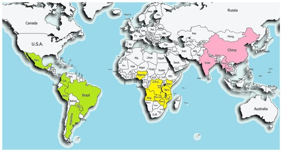
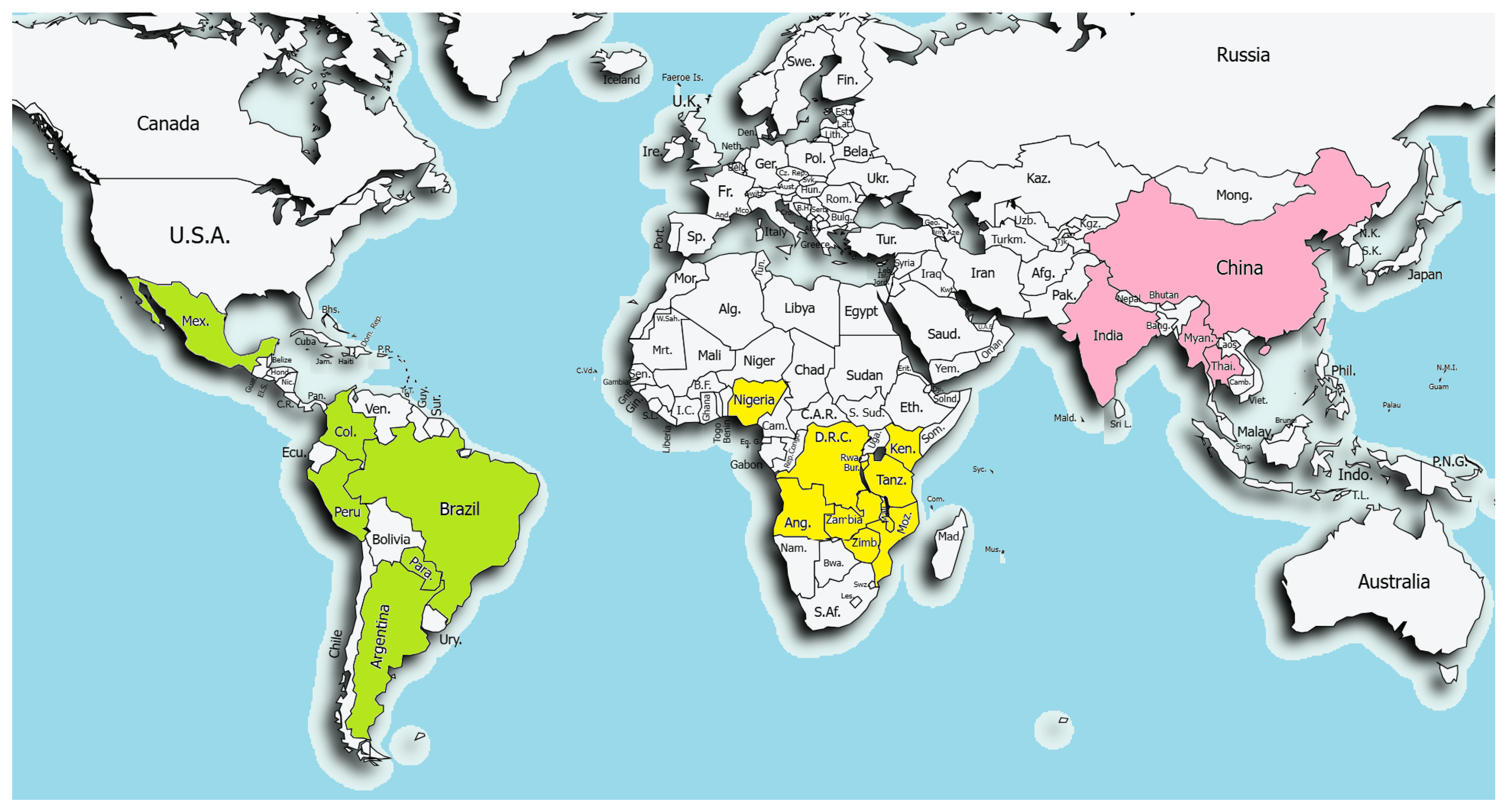
The chosen 20 countries account for 25.9% of global wheat area, 35.1% of wheat production, 73.2% of cassava area, and 64.6% of cassava production. They cover more than 89% of their respective regions, both in output and in harvested area. This substantial share ensures the global relevance and validity of the panel. The chosen countries provide a nearly balanced panel, i.e., 1961–2024 = 64 years of data for 2 crops =128 observations per country. The only exception is Thailand, a significant cassava producer with rather low wheat production, for which wheat data are unavailable from 1961 to 1985. However, it is included in the model because of its significance in cassava production within Asia. The only missing data are those of Thailand’s wheat yield and area from 1961 to 1985, and these cases were omitted from the analysis. Figure 1 shows the location of the 20 selected countries, with 6 in Latin-America, 10 in Africa, and 4 in Asia.
Figure 1.
Countries included in the analysis (authors’ own construction based on the blank map available at https://paintmaps.com/blank-maps/293/World-blank-map-maker) (accessed on 10 August 2026).
Table 3 lists the variable names, meanings, and sources. The dataset integrates temporal tracking (YEAR/YearC), geographic indicators (Region, ISO3, CountryName), quarterly climate anomalies (TMS1–S4 for temperature, PrecS1–S4 for precipitation), physical crop yields (including lags), and harvested areas. Seasonal temperature and precipitation values were computed from monthly values averaging the three months of the meteorological seasons (S1: March–April–May; S2: June–July–August; S3: Sept–Oct–Nov; S4: Dec–Jan–Feb). Although these fixed seasons introduce minor mismatches with local planting calendars (e.g., winter wheat in India) and cassava’s longer 12–24-month cycle, a standardized seasonal baseline was maintained to ensure a consistent, direct comparative analysis between the two crops across all studied macro-regions. Anomalies were computed by comparing the actual seasonal value to the 30-year average of the same season in the 1951–80 baseline period: temperature anomaly for a season was the actual seasonal value minus the 30-year baseline of the same season; relative precipitation anomaly of a season was the actual seasonal precipitation minus the 30-year baseline of the same season, divided by the 30-year baseline of the same season. The anomalies and the relative anomalies are therefore centred around zero, and their magnitudes vary between −1.95 and +2.69 for temperature, and −0.9 and +2.9 for precipitation, a comparable magnitude to the other variables in the model. These anomaly computations are widely used in climate analyses [1,2,3].
Table 3.
The variables used for the analysis.
2.3. Statistical Analyses
For the analysis, two approaches were used: machine learning random forest regression and the linear mixed-model panel regression. As previously mentioned, the two main analysis methods for crop–climate relationships are the process-based crop models based on causal relationships between crop yield and environmental inputs, and the statistical models, establishing econometric relationships, usually by regression, between historical crop yields and environmental data [63,64,65,66]. However, process-based crop models require intensive data and calibration, while statistical models establish simple but reasonable relationships that are limited only within the range of the historical data. Statistical modelling methods based on machine learning algorithms can provide alternatives to traditional regression approaches, overcoming some of their limitations [66]. These techniques assume the data mechanism as a ‘black box’ or ‘grey box’ and have been adopted widely, either for classification or for prediction [66,67,68,69,70]. They have outstanding predictive strengths, with high precision, handling automatically and efficiently the complex and non-linear interactions between variables and multicollinearity, as the explanatory variables, such as heat and drought, are strongly correlated [71,72].
2.3.1. Machine Learning Random Forest Regression
We take a set of predictor variables and a number of historical cases (rows) for these variables. To strictly prevent any data leakage due to the lagged variables in our panel structure, these cases are divided using a chronologically structured, time-based split. Using the training set, the algorithm creates a collection of individual decision trees (the random forest). Accordingly, the first year (1961) was omitted from the database to construct the lag, and the training set used the first 51 years (1962–2012) as the historical training period, and the remaining 12 years (2013–2024) were used as the out-of-time test set. As a tree grows, at every single split point, a small subset of the predictor variables (e.g., PrecS1, TMS1, TMS2, etc.) is randomly selected. The tree evaluates these chosen variables and creates a split based on a specific threshold (i.e., PrecS1 < 0.5 or not), evaluating the crop yield within each resulting subset. If the yield is still highly varied within a subset, further splits are made by newly selected random variables (e.g., taking WhAr for the next split, splitting by PrecS1 further). This splitting continues down the branches until a tree reaches its final predicted crop yield. This procedure is repeated independently to develop all the decision trees, creating the random forest. When a new case of predictor variables is received, the random forest runs those values down the relevant branches of every single decision tree. The final prediction is the mathematical average of the individual predictions of all the decision trees. Finally, taking the test set, not yet used in the model development, the same decision rules are applied to predict the crop yield. Comparing this prediction to the actual real-world values, the model’s true real-world accuracy score is computed. The relative importance of the predictor variables is assessed by computing several feature-importance indicators, such as the Mean Decrease in Accuracy, or the RMSE and R2 values on the test set. To interpret the model, Shapley Additive Explanations (SHAP) is used to measure the marginal contribution of each feature to the model output. To validate the reliability of the computations, the leave-one-country-out procedure is applied. During this iterative procedure, the model is developed on a training set, omitting a country, and then it is tested strictly on that omitted country. Therefore, the country identifier is excluded from the predictor set during this procedure, forcing the model to generate predictions based on the remaining variables. This is repeated for each of the 20 countries, and the final performance is evaluated by averaging the test RMSE and R2 values across the 20 countries.
ML-RF was applied to compare the weather dependence of wheat and cassava yields, ranking the importance of weather variables and other predictors, such as Year, Country, Region, and crop harvested area.
2.3.2. Panel Regression and Diagnostics for the LMM-FE and LMM-RE Model
Panel regression was applied to determine the direction and magnitude of the associations between weather and yield variables for the two crops separately, comparing them to see whether these relationships differ considerably between the two crops.
Since the database has a panel structure, with repeated, time-series observations of 20 countries over 64 years, the observations are not independent. To handle within-country autocorrelation and the nested structure, a Linear Mixed Model (LMM) was specified, which contains random effects in addition to fixed effects. The application of an LMM instead of a Generalized Linear Mixed Model (GLMM) is justified when the dependent variable is continuous (GLMM is applied with binary success/failure or count data with a Poisson distribution) and when the residuals of the LMM are close to the normal distribution [73] or, in the presence of heavy-tailed residuals, when the model employs the Satterthwaite degrees of freedom adjustment [74,75] to ensure robust statistical inference. To control for unobserved time-specific common shocks affecting all countries simultaneously (e.g., El Niño events or global crises), time fixed effects (year dummies) are explicitly included in the model. The application of the Satterthwaite [74] approximation can reliably safeguard statistical inference against small-cluster bias given our sample size (N = 20).
The statistical correctness of applying the LMM (Linear Mixed Model) can be best justified by the following steps.
The LMM, incorporating Country as a random grouping factor, can handle within-cluster correlation [73]. The ICC (Intraclass Correlation Coefficient) value for the clustering variable (country) substantially greater than 0 (e.g., above 0.15) means that a significant portion of the data’s variance stems from group membership, further supporting the LMM configuration [74,75]. The diagnostic procedures refer to autocorrelation, multicollinearity, heteroskedasticity, and the reliability of the FE (fixed effect) or RE (random effect) configuration. To account for autocorrelation, the one-lagged value of the dependent variable is added as a predictor in the model. Multicollinearity is checked by computing the Variance Inflation Factor (VIF) [76]. To account for other issues of model validity, a Mundlak specification was introduced [76,77].
To decide whether a Random Effects LMM (LMM-RE) or a Fixed Effects LMM (LMM-FE) is appropriate, the following diagnostics are applied. The FE model assigns a unique baseline value to every single group (e.g., every country). Because of this, important explanatory variables that are constant at the group level drop out of the FE model entirely, because FE “filters out” all between-group variance. The statistical tests for evaluating the appropriateness of these models are the Hausman test and the more robust Mundlak test [76,77]. The null hypothesis of these tests is that the random effects are uncorrelated with the explanatory variables, meaning that the RE model provides unbiased estimates. A small p-value (below 0.05) rejects this null hypothesis, indicating that the RE assumption fails and therefore the FE model must be used to ensure unbiased estimates. Conversely, a large p-value (above 0.05) fails to reject the null hypothesis, suggesting that the RE model is appropriate due to its higher efficiency.
The LMM for a panel with cross-sectional and longitudinal data allows for regulatory unobserved heterogeneity across cross-sectional units (e.g., country-specific fixed features, like persistent soil quality, institutional context, and management style) and for chronological trends affecting all countries. Our panel model is formulated as:
where i denotes countries, and t denotes time (years). LnCropYit denotes LnWhYit in the wheat model and LnCassYit in the cassava model.
LnCropYit = α + Xitβ + Zitγ + µi + vit i = 1, …, n, t = 1, …, T
The parameter α represents the overall grand mean for all countries and years, µi represents the i-th time-invariant country effect, while vit is the error component, assumed to have zero expected value. The matrix Xit contains the weather-related predictor vectors (TMS1it, …TMS4it, PrecS1it, …, PrecS4it), and the vector β contains the coefficients describing the effects of these predictor vectors on the dependent variable. The matrix Zit contains the control variables, namely WhArit, LnWhYLagit and YearCit in the wheat model and CassArit, LnCasYLagit and YearCit in the cassava model, and the vector γ contains the coefficients describing the effects of these predictor vectors on the dependent variable [77].
A fixed-effects model assumes that the µi intercepts are fixed values and do not vary by time, and that they can correlate with the Xit and Zit predictor matrices. A random effects model, however, assumes that the µi values are random values and are strictly uncorrelated with Xit, Zit, and the error term. In the fixed-effects model, it is common to take the overall intercept as the mean of the individual effects; therefore, the formula may contain this overall intercept, and the individual effects can represent deviations from this overall mean. However, in the random effects model, the individual deviations around the overall mean are not fixed but random values from a specific distribution.
The Hausman test is the usual tool to test whether the fixed effect model or the random effect model is appropriate. However, when the homoskedasticity of the variables cannot be assumed, the Mundlak test is a more robust version. The Mundlak test has a null hypothesis that the estimated coefficients of the panel-level means are jointly zero, implying no correlation between the time-invariant unobserved heterogeneity and the regressors. It is reliable even when errors exhibit heteroskedasticity or serial correlation. A significant test value, i.e., a small p-value, suggests that the null hypothesis is rejected, indicating that the random-effects assumption fails due to endogeneity, thereby necessitating the use of the fixed-effects model to obtain unbiased estimates.
Therefore, in addition to a simple LMM structure, the more refined Mundlak specification is applied, as it facilitates the explicit decomposition of the effects into within-country and between-country components, addressing concerns about time invariance and the potential correlation with country-level unobserved heterogeneity. The Mundlak specification includes country-level means of the key regressors alongside their within-country deviations and relaxes the strict exogeneity assumption of the standard random-effects model. It can assess whether the estimated effects are primarily driven by between-country differences or within-country variations. So, to separate these effects, a hybrid panel approach, proposed by Mundlak [77], was employed, as was applied, for example, by Wooldridge [76] and Bell & Jones [78]. The within-country variation captures temporal changes within a country, while the between-country variation reflects structural differences across countries. The model equation is:
where the notations are the same as in Equation (3), while matrix XMi denotes the 64-year averages of the weather variables for each country, and δ is the estimated parameter vector of these averages.
LnCropYit = α + Xitβ + XMiδ + Zitγ + µi + vit, i = 1, …, n, t = 1, …, T.
The Mundlak specification is applied in panel econometrics to control time-invariant heterogeneity, though time-varying omitted variables may still remain. The Mundlak approach eliminates time-invariant heterogeneity by decomposing the explanatory variables into between-group and within-group components. The group mean included in the model acts as a control variable, capturing and neutralizing the effects of unobserved, time-invariant individual characteristics (e.g., institutional culture), leaving the coefficient of the original variable free from biases stemming from time-invariant omitted variables, ensuring that group-level endogeneity is resolved.
The machine learning computations were performed by Orange V 3.40 [79], while the LMM computations were performed by Stata V16 [80] and JASP V0.98 [81].
3. Results
3.1. Descriptive Statistics
The main descriptive metrics (mean, standard deviation, skewness, kurtosis, and range) are computed across 1280 total observations (Table 4). A systematic warming trend is visible across all seasons, with mean temperature anomalies around +0.35 °C. The negative mean precipitation anomalies suggest drying across all seasons, especially in S1 and S4. The 25 missing values in the wheat yield variable (LnWhY) are exclusively due to historical data gaps for Thailand between 1961 and 1985.
Table 4.
Descriptive statistics of the variables (20 countries, 64 years).
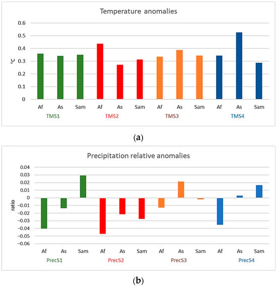
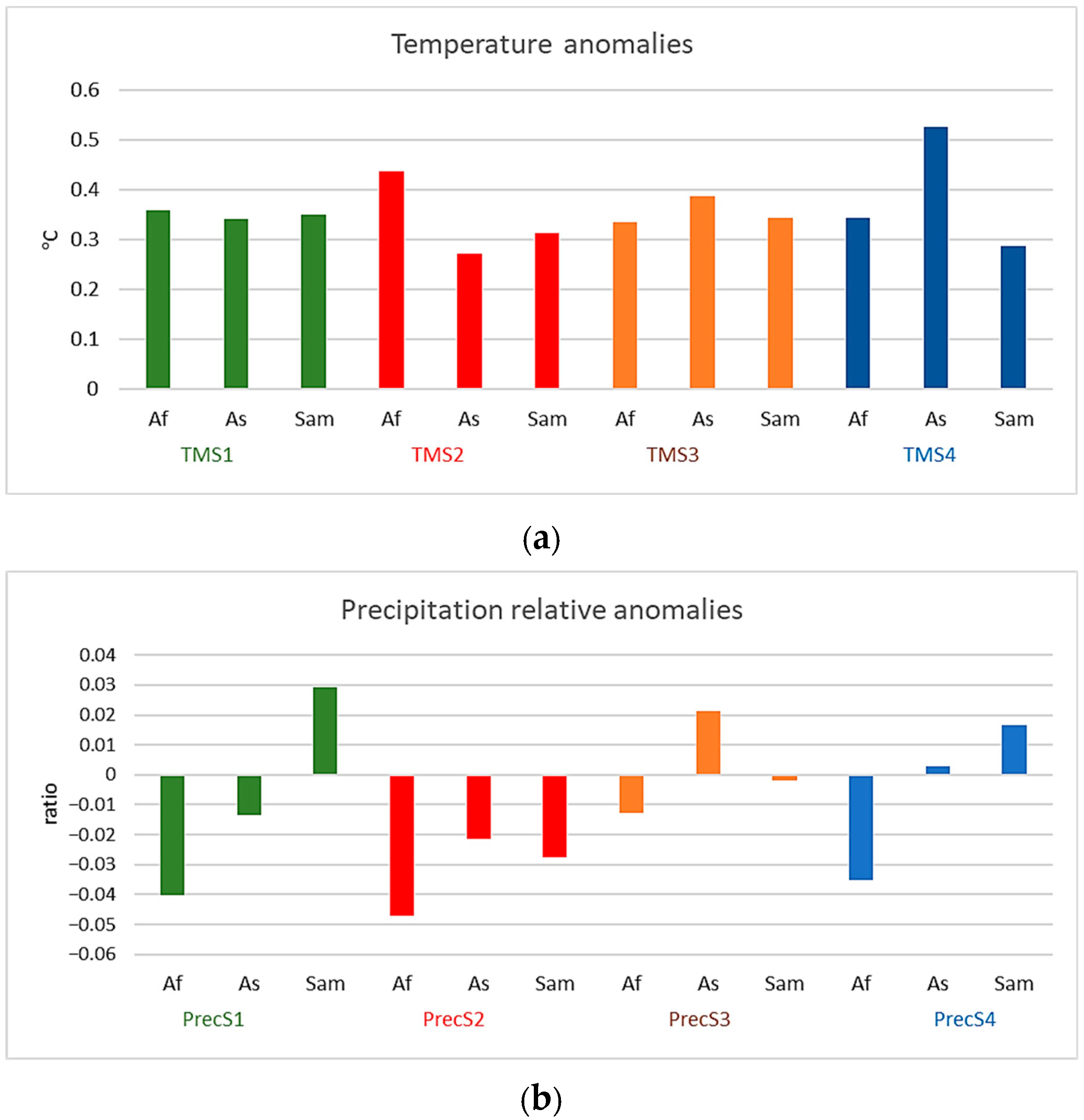
Table 5 and Figure 2 present the region-wise averages, with analysis of variance among the three geographic regions (Africa, Asia and Pacific, and Central and South America) by the Tukey post hoc test. Climate pressures differ significantly by geography. Africa exhibits the highest temperature anomalies in Season 2, and Asia experiences extreme warming in Season 4, while Central and South America shows uniquely higher, positive relative precipitation anomalies in Season 1. Africa has the most negative precipitation anomalies in every season, being the only continent with no positive values.
Table 5.
Comparison of regions by climate variables.
Figure 2.
64-year means of variables by region: (a) Seasonal mean temperature anomalies; (b) seasonal precipitation relative anomalies.
3.2. Machine Learning—Random Forest Estimation Results
The random forest regression was performed separately for cassava and wheat. Table 6 presents the results, listing the target variable and the predictor variables for the two crops.
Table 6.
Machine learning random forest feature importance table for cassava.
As Table 6 demonstrates, the highest feature importance scores are attributed to the lagged yield, followed by the country, the crop area, and the year. Region is also among the most important features for cassava, while its importance in wheat yield is considerably smaller. The weather variables show much less importance than the previous year’s yield, harvested area, or the year. The reliability of the prediction is quite strong, with R2 = 0.893 for cassava and R2 = 0.853 for wheat. The leave-one-country-out diagnostics show that these effects are fairly general, and the average R2 values are also quite high, 0.801 for cassava and 0.742 for wheat.
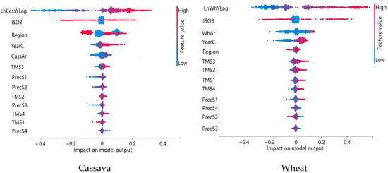
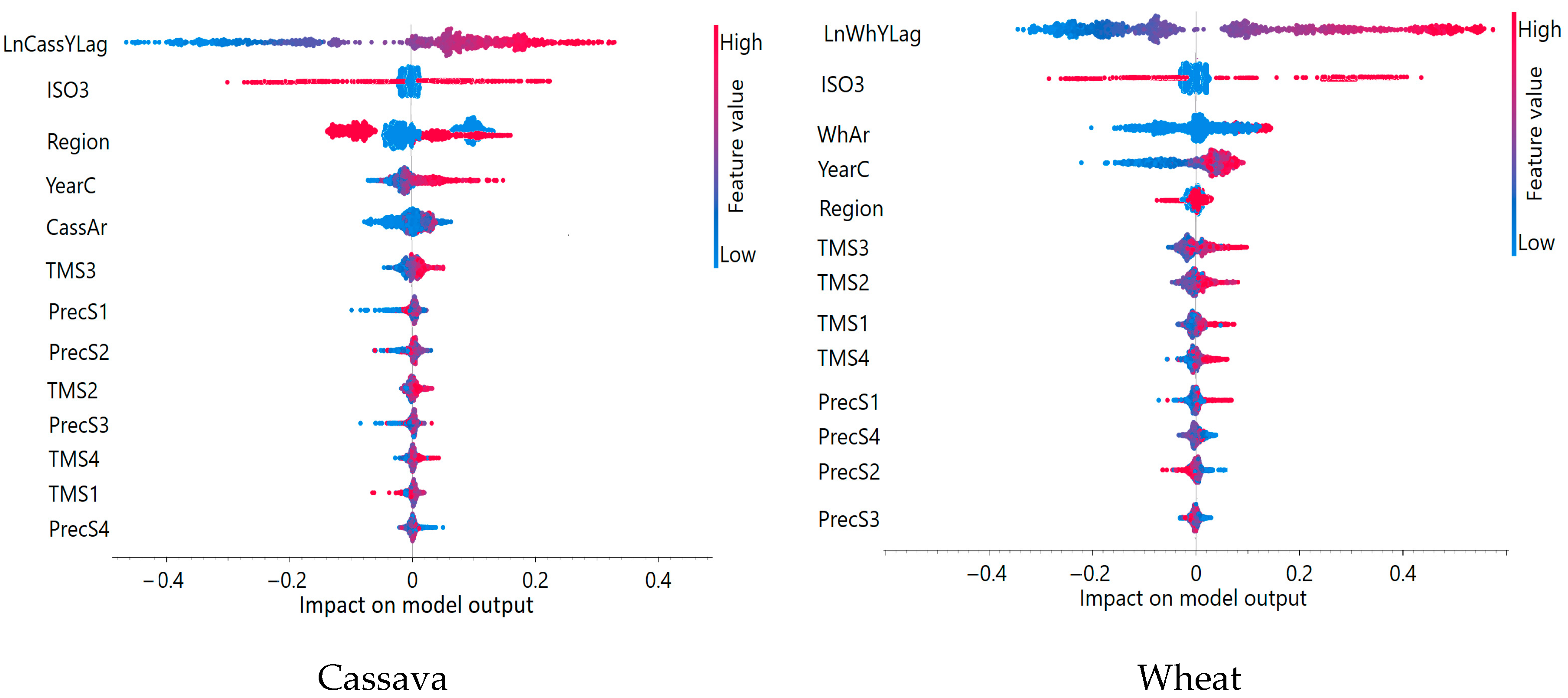
Similarly, the SHAP plots (Figure 3) also highlight the differences between cassava and wheat. While the lagged dependent variables (LnCassYLag and LnWhYLag) are the most dominant predictors, i.e., past yields fundamentally drive current yields for both crops, country differences are also important, while regional differences matter much more for cassava than for wheat.
Figure 3.
Shapley diagram for cassava (left panel) and wheat (right panel) prepared using Orange V3.40 [79].
For both crops, meteorological variables (temperature and precipitation anomalies) exhibit highly uniform patterns, clustering tightly around zero with narrow, symmetric distributions.
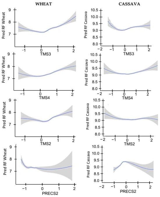
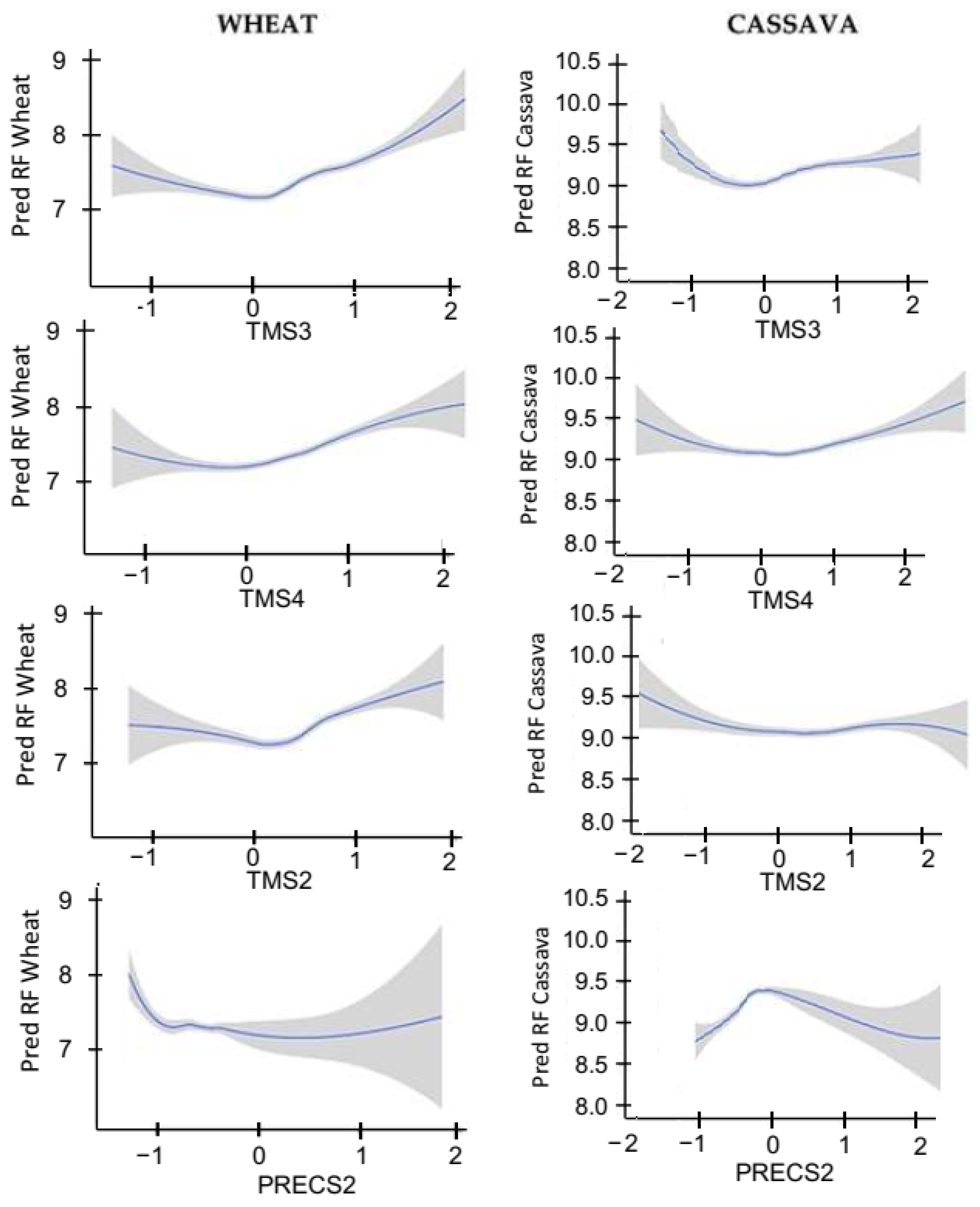
To capture the exact non-linear behaviour and threshold effects of the weather anomalies, Figure 4 plots the random forest predicted values (Pred RF Wheat and Pred RF Cassava) against the key quarterly climate anomalies (TMS2, TMS3, TMS4, and PrecS2) to reveal the non-linear dynamics of the model.
Figure 4.
The partial dependence plots for the main weather predictors for the wheat and cassava random forest models.
For wheat, both TMS3 and TMS4 graphs show a sharp upward trend, where extremely positive S4 temperature anomalies (TMS4) are linked to higher predicted yields. The only severe drop appears at the early phase of the PrecS2 curve. Cassava precipitation (PrecS2) exhibits a clear inverted U-shaped curve, peaking exactly at 0 (baseline precipitation) and dropping significantly during both drought and excessive rainfall. The temperature curves (TMS3 and TMS4) display a slightly U-shaped behaviour where extremely positive anomalies correspond to higher predicted yields. These curves include confidence bands (grey shaded areas) to illustrate prediction uncertainty.
3.3. Panel Regression Results
Table 7 presents the simple LMM panel model estimates. For wheat, Season 2 temperature (TMS2) is significantly negatively associated with yield (−0.0456, p = 0.0049), while YearC and yield lag are strongly positive. For cassava, weather anomalies show no significant associations (except for marginally positive PrecS1); yield lag (0.9285) dominates the model, YearC is significantly positive, and area (CassAr) is negative.
Table 7.
LMM summary for wheat and cassava.
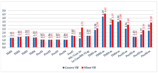
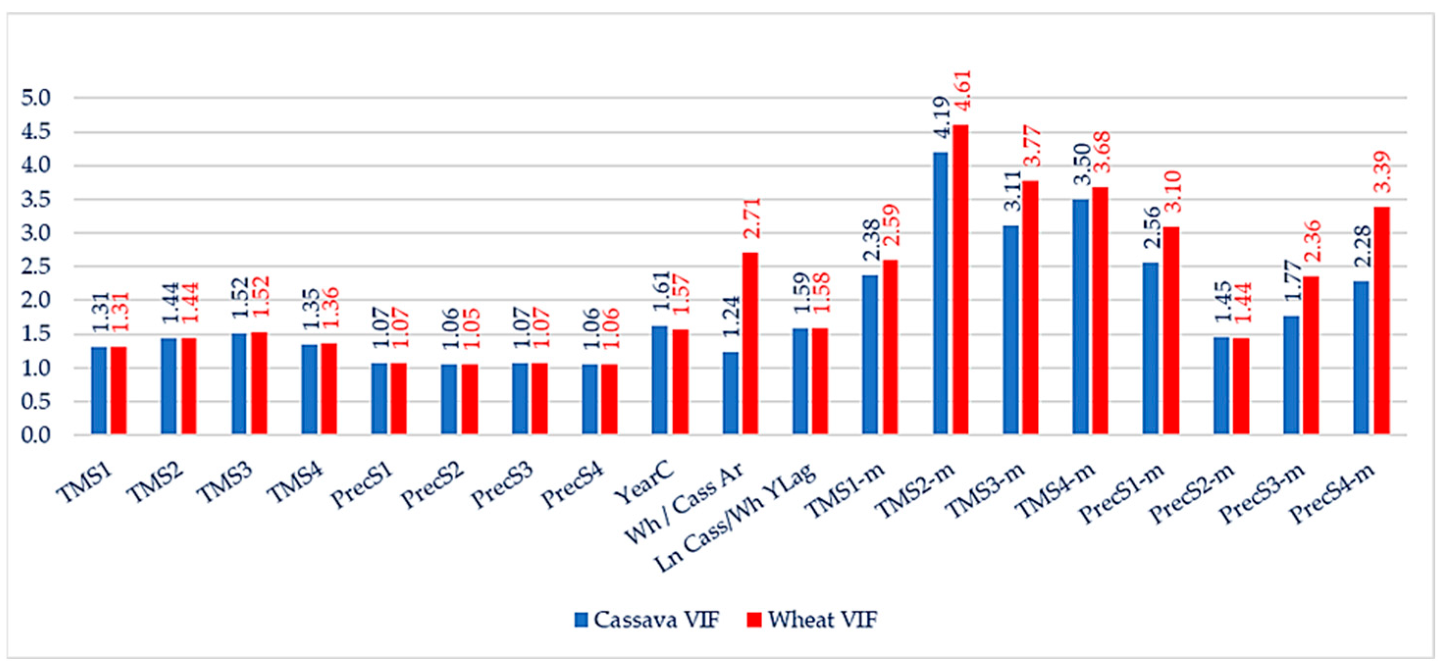
The multicollinearity test results (Figure 5) show all VIFs well below 5.0, and there is no issue of multicollinearity in the model.
Figure 5.
The VIF values for the LMM of the cassava and the wheat model.
The Mundlak-type model was also set up and run for both crops, adding the country-specific historical means (denoted by “-m” after the variable name) to the previous LMM specification to capture within- versus between-country variations (Table 8).
Table 8.
The Mundlak-type LMM for wheat and cassava.
For wheat, there are three Mundlak variables that are statistically significant (TMS2-m, PRecS1-m, and PrecS4-m); therefore, the RE model assumptions fail, so the Mundlak-type model is the only reliable model version to use. For cassava, there is one Mundlak variable that is statistically significant (TMS2-m), while TMS3-m is also at the border of 5% significance; therefore, the RE model assumptions fail.
The last two rows in Table 8 present the Mundlak test, a formal likelihood-ratio test comparing the simple LMMs against the Mundlak-type specifications. This test is superior to the usual Hausman test, as it is not sensitive to violations of distribution assumptions. The p-values for both crops are well below the critical 0.05 threshold (wheat: p = 0.000192, cassava: p = 0.026634), mathematically rejecting the standard random effects framework. Thus, the Mundlak-type model is the correct, statistically unbiased, reliable parametric specification to use for this panel.
The column ‘% effect’ translates the β coefficients to percentage changes: percentage change in yield = (eβ − 1) × 100%, for the significant predictors. Thus, a one-unit change in the predictor changes the yield by the percentage shown in the ‘% change’ column. Therefore, wheat exhibits a more than 4% yield decrease for any 1 °C warming in Season 2, while cassava yield is not related to it. A relative precipitation increase of one unit in Season 1 (i.e., a doubling of the seasonal precipitation) aligns with a 5.77% yield increase in wheat and a 3.32% increase in cassava, or a 0.1 unit increase in relative anomaly aligns with a 0.577% yield increase in wheat and a 0.332% yield increase in cassava (although it is significant only at the 10% level), and the relationship of precipitation decrease is just the opposite. Regions with historically 1 °C warmer Season 2 (June to August) enjoy 154.16% higher wheat yields, but 28.84% lower cassava yields. Historically warmer Season 3 (September to November) experiences 58.68% lower wheat yields per 1 °C, but 56.16% higher cassava yields (significant only at 10% level). Historically, a one-unit higher relative precipitation anomaly in Season 1 (March to May) shows 3.99% higher wheat yields, while a one-unit higher relative precipitation anomaly in Season 4 (December to February) shows mildly lower wheat yields (−2.0%), while cassava does not show any relationship to historical precipitation averages in any season. Harvested area shows a significant positive relationship with wheat, a unit (1 million ha) increase in harvested area being associated with a 0.90% yield increase, while a negative relationship is exhibited for cassava (a one-unit area increase aligning with a 1.33% yield decrease). A unit increase in the ln-transformed yield of the previous year is related to 116.85% higher wheat yield, or a 1% higher yield in the previous year aligns with a 0.77% yield increase in the current year. Similarly, a 1% higher cassava yield in the previous year is associated with a 0.90% higher cassava yield in the current year. Finally, the temporal trend (YearC) shows an annual yield increase of 0.30% for wheat, and by 0.10% for cassava. Therefore the following two equations hold (‘[ ]’ indicating significance only at 10%):
LnWhY = 1.4497 − 0.0459 × (TMS2) + [0.0561 × (PrecS1)] + 0.0029 × (YearC) + 0.0090 × (WhAr) + 0.7745 × (LnWhYLag) + 0.9328 × (TMS2 − m) − [0.8839 × (TMS3 − m)] + 0.0391 × (PrecS1 − m) − 0.2020 × (PrecS4 − m) + country intercept + error term
LnCassY = 0.8575 + [0.0327 (PrecS1)] × 0.0010 × (YearC) − 0.0134 × (CassAr) + 0.9032 × (LnCassYLag) − 0.3403 × (TMS2 − m) − [0.4451 × (TMS3 − m)] + country intercept + error term
4. Discussion
The random forest models show that farm management, history, and location set the basic yield level, while the final yearly harvest varies mostly by specific weather conditions during the season.
For both cassava and wheat, the previous year’s yield and country identity (LnCassYLag, LnWhYLag and ISO3) are the most powerful predictors, reflecting agricultural inertia. A country with high-input wheat systems (like China or India) maintains a structural advantage over low-input systems regardless of minor annual weather fluctuations. Table 7 and Table 8 show a clear positive tendency when wheat harvested areas expand (WhAr) and a clear negative tendency when cassava areas expand (CassAr). This may be related to the fact that wheat is often a commercial commodity backed by technological intensification, modern inputs, and irrigation, while cassava area expansion is more frequently driven by subsistence farming, pushing the crop onto inferior, nutrient-poor marginal lands, and thereby decreasing average productivity, although our model did not evaluate these factors.
The positive relationship between yield and year (YearC) represents a continuous, long-term temporal trend. While year is traditionally associated with technological advancement, like gradual adoption of high-yielding varieties, synthetic fertilizers, and expanded irrigation, it must be interpreted cautiously. Agronomically, this linear trend operates as a proxy for a bundle of time-varying factors, like mechanical and genetic progress, structural shifts in global agricultural policies, long-term changes in atmospheric carbon-dioxide fertilization effects, institutional improvements in extension services, and systematic changes in farm management practices over the 64-year timeline.
The Mundlak models that separate long-term regional climate baselines (between-country differences reflected by the ‘-m’ variables) from short-term annual shocks (within-country anomalies) reveal interesting differences between wheat and cassava.
Our statistical analysis indicates that S2 (Jun–Aug) temperature negatively impacts wheat yields (every 1 °C warming exhibiting a 4.49% decrease in yield), whereas S4 (Dec–Feb) precipitation exerts a marginally positive effect on both wheat (5.77% yield increase when precipitation anomaly increases by 1 unit compared to the baseline) and cassava (3.32% yield increase). Furthermore, the Mundlak-transformed country means differ considerably between the two crops. While for wheat the higher long-term temperatures in Season 2 align with much higher yields (every 1 °C warming exhibiting a 154.16% higher yields), the same warming for cassava is associated with lower yields (28.84% decrease for 1 °C warming). An opposite, though only marginally significant, relationship is shown for the long-term temperatures in Season 3 (Sept–Nov) for both crops. However, cassava yields are unrelated to long-term precipitation anomalies, while higher precipitation in Season 1 (March–May) aligns with higher yields (a unit increase in precipitation anomaly compared to the baseline is associated with 3.99% yield increase), and a unit increase in precipitation anomaly in Season 4 (Dec–Feb) aligns with 2% yield decrease. The physiological and agro-meteorological mechanisms diverge by hemisphere. In the Southern Hemisphere (e.g., Brazil and Argentina), S2 corresponds to the winter vegetative and tillering stages; anomalous warmth during this window accelerates crop development, restricting tiller formation and spike density. In the Northern Hemisphere (e.g., China, India), where winter wheat has already been harvested, high S2 summer heat induces severe soil moisture depletion through enhanced evapotranspiration and limits the baseline moisture available for the subsequent autumn planting cycle. Conversely, S4 precipitation is highly beneficial across regimes: it provides vital moisture for active winter crop growth in South Asia (e.g., India) and marks the peak of the tropical wet season in the Southern Hemisphere (e.g., Congo and Brazil), maximizing the cassava canopy development required for subsequent root bulking. The opposite signs in the Mundlak regression about Season 2 temperature for wheat highlight the distinction between short-term weather shocks and long-term climate adaptation. The negative within-country coefficient reveals that unexpected June–August heat anomalies above the historical baseline directly harm wheat yields, while the positive long-term group-mean coefficient suggests that countries with historically higher seasonal temperatures achieve higher yields due to structural and technological adaptation, such as heat-tolerant crop varieties.
These estimation results reveal basic differences in climate sensitivity between cassava and wheat. While wheat is considerably more sensitive to short-term temperature shocks in Season 2, it prefers regions where Season 2 is warmer in the long term and Season 1 is wetter, and it suffers in areas where Season 3 is warmer and Season 4 is wetter. Cassava, on the contrary, suffers in regions with higher long-term Season 2 temperatures, but does not seem to be sensitive to short-term shocks and precipitation differences. The positive coefficient of the lagged dependent variable (for both wheat and cassava) shows that a good harvest last year naturally boosts this year’s yield because it leaves the soil more fertile and gives farmers more money to buy better seeds and fertilizers.
Our empirical findings strongly support the established literature regarding the divergent climate vulnerabilities of these two C3 staples. For wheat, the highly significant within-country negative impact of short-term summer warming (TMS2 = −0.0459, p = 0.0048) reinforces the consensus that heat stress acts as a dominant constraint over seasonal precipitation anomalies. This severe sensitivity to short-term temperature shocks aligns closely with the foundational assessments by Asseng et al. [16], Liu et al. [82], and Lobell et al. [83], which demonstrated how terminal heat waves accelerate leaf senescence and restrict the critical grain-filling window in temperate cereals. Conversely, for cassava, the complete absence of statistically significant linear yield depressions from single-year seasonal weather shocks (TMS1–S4 and PrecS1–S4) empirically verifies the crop’s robust biological buffering capacity under contemporary weather transitions. This definite resilience under transient climate stress is consistent with the strategic role of cassava as an atmospheric buffer crop outlined by Jarvis et al. [15]. Furthermore, this short-term insensitivity supports the physiological mechanisms detailed by Leakey et al. [4] and Ruiz-Vera et al. [19], who observed that cassava possesses highly efficient adaptive mechanisms, such as optimized stomatal regulation, to maintain subterranean tuber development even during active moisture deficits. However, our Mundlak specification reveals an important nuance: while cassava effectively buffers against localized annual volatility, its long-run productivity remains rigidly bound to structural regional baseline climates, as evidenced by the high significance of the long-term temperature mean anomaly (TMS1-m = 0.3489, p = 0.0178) and relative precipitation anomaly (PrecS4-m = 0.9258, p < 0.0001). These structural parameters indicate that permanent shifts in regional temperature regimes fundamentally alter biomass growth over the long run, mirroring the long-term vegetative and respiratory trade-offs discussed by Rosenthal et al. [18] and Asseng et al. [16].
However, cassava’s response to climate change is not uniform; genotype significantly determines resilience. In a study [84], cassava, examined at 23 °C and 34 °C under well-watered conditions and after a one-month drought treatment, showed reduced growth and tuber yield due to drought, while its concentration of cyanogenic compounds increased. The combination of high temperature and drought exerted a stronger negative impact on tuber yield than drought alone. A 28-day water deficit was applied in an experiment in another study [85], with the result of 83% lower tuber yield, a 45% loss of leaves, and quadrupled concentration of cyanogenic compounds in the tubers, leading not only to less crop quantity but also deteriorating food safety and quality. Another recent study [86] compared 37 cassava genotypes under field conditions, finding that under drought, on average, yield decreased by 59%, the number of edible storage roots decreased by 43%, and leaf retention decreased by 50%. Moreover, there were massive differences among genotypes; the most drought-tolerant genotype yielded 7.1 t/ha under drought, while the most sensitive yielded only 3.3 t/ha. Heat stress can also affect cassava adversely, as was established in an experiment [87] testing the effects of 15 °C and 45 °C temperatures on the crop. At 45 °C, net photosynthesis decreased by approximately 50% compared to the 30 °C treatment. Although cassava is indeed a warmth-loving plant, it may not tolerate temperature increases indefinitely, and above an optimal range, its physiological performance deteriorates. In an experiment working with climate scenarios simulating conditions in southeast Brazil [88], the findings indicated that climate change could lead to a cassava yield loss of approximately 8.6 and 9.7 t/ha, respectively.
Limitations of the study: Our empirical research dealt with seasonal weather data, and although this treatment can reflect the most sensitive phenological stages of the two crops, more detailed (e.g., monthly) data may give more refined results. While fixed meteorological seasons do not perfectly align with every local crop calendar (e.g., wheat in India or cassava’s 12–24-month cycle), they provide a standardized, uniform baseline that is necessary for a direct cross-crop comparative analysis across macro-regions. The other limitation is that the countries are handled as homogeneous regions. This may be reasonable for small areas, but countries like China and India, with their vast territories, can experience diverse weather patterns across their regions. Further research may deal with crop-specific regions within countries and seasons more finely tuned to the crop growth stages in these areas. Another refinement could be to analyze yield data of different cassava and wheat varieties, adding other omitted agronomic variables (irrigation, fertilization, pest and disease management), to assess their different responses to changing weather factors. Further research can be developed in this direction depending on data availability. However, long-term cross-country institutional and structural differences (e.g., historical irrigation infrastructure, average soil degradation, and baseline policy regimes) were successfully captured by the Mundlak components (historical country means), and time-varying technological progress (e.g., fertilizer intensity, machinery adoption, and improved varieties) was captured by the lagged dependent variable, which reflects the cumulative agronomic and socio-economic trends of each nation up to the previous year. This structured framework ensures that our primary weather coefficients isolate the clean, contemporary meteorological shocks, uncorrupted by long-term non-climatic trends.
5. Conclusions
This study demonstrates the value of combining machine learning (random forest) with robust econometric specifications (Mundlak-type Linear Mixed Models) to untangle the complex effects of climate anomalies on global crop yields. The empirical evidence indicates a notable variation in climate vulnerability between wheat and cassava within the analyzed balanced panel. Long-term trends and stable country-specific factors tend to shape baseline productivity, while short-term seasonal climate anomalies potentially influence year-to-year variation in annual yields. Methodologically, the rejection of the standard random effects model via the Mundlak test highlights that analyzing climate impacts without accounting for unobserved country heterogeneity and structural variations in regional features leads to biased interpretations.
From an agronomic viewpoint, we may conclude that wheat exhibits severe sensitivity to contemporary climate volatility. It faces immediate threats from summer heat shocks (Season 2) above the long-term averages, while regions with generally warmer climates achieve higher wheat yields, which may be due to structural and technological adaptation, including yield varieties. Conversely, cassava demonstrates remarkable biological resilience against year-to-year weather shocks, showing no linear yield depression to single-year climate anomalies. However, cassava’s productivity remains tightly bound to long-term climate shifts, as structurally hotter baselines alter its growth dynamics. Therefore, while cassava serves as a vital buffer crop against immediate seasonal volatility, permanent shifts in regional climate baselines present a profound, long-term risk to both crops. Consequently, while cassava’s resilient root system could offer a strategic buffer against rising temperatures and drier summers in mid-latitude zones, its long-term success remains fundamentally constrained by permanent shifts in regional climate baselines.
Based on these findings, target-oriented policy interventions should focus primarily on mitigating seasonal climate constraints for wheat and on accounting for the opposing land-expansion dynamics observed between the two crops. For wheat production, investment should prioritize institutional support to manage thermal stress during sensitive seasons and enhance water management practices to buffer against rainfall deficits. For cassava, the significant negative relationship between harvested area and yield suggests that horizontal land expansion restrains average productivity, likely due to the cultivation of marginal, lower-quality soils. Therefore, regional agricultural planning should shift its focus away from extensive land expansion for cassava toward localized, climate-smart extension services that promote yield-improving management on existing plots.
Author Contributions
Conceptualization, Z.B., H.M.A., and D.D.J.; methodology, Z.B., H.M.A., and D.D.J.; software, Z.B., H.M.A., and D.D.J.; validation, Z.B., H.M.A., and D.D.J.; formal analysis, Z.B. and H.M.A.; investigation, Z.B. and D.D.J.; resources, Z.B.; data curation, H.M.A. and D.D.J.; writing—original draft preparation, Z.B. and D.D.J.; writing—review and editing, Z.B., H.M.A., and D.D.J.; visualization, Z.B.; supervision, Z.B.; project administration, Z.B.; All authors have read and agreed to the published version of the manuscript.
Funding
This research received no external funding.
Data Availability Statement
Data derived from public domain resources. The data presented in this study are available in: FAOSTAT-Crops and Livestock Products data: https://www.fao.org/faostat/en/#data/QCL (accessed on 28 January 2026); Climatic Research Unit, University of East Anglia, CRU-CY v4.10 tmp: Country-averaged monthly climate data, 1901–2025. University of East Anglia. 2026. https://crudata.uea.ac.uk/cru/data/hrg/cru_ts_4.10/crucy.2606161920.v4.10/countries/tmp/ (accessed on 22 August 2026); and Climatic Research Unit, University of East Anglia, CRU-CY v4.10 pre: Country-averaged monthly climate data, 1901–2025. University of East Anglia. UK. 2026. https://crudata.uea.ac.uk/cru/data/hrg/cru_ts_4.10/crucy.2606161920.v4.10/countries/pre/ (accessed on 22 August 2026).
Conflicts of Interest
The authors declare no conflicts of interest.
Appendix A
Table A1.
The 2021–2024 mean area and production for wheat and cassava as % of world average, including 36 countries.
References
- IPCC. Climate Change 2022: Impacts, Adaptation, and Vulnerability. Contribution of Working Group II to the Sixth Assessment Report of the Intergovernmental Panel on Climate Change; Cambridge University Press: Cambridge, UK; New York, NY, USA, 2022. [Google Scholar] [CrossRef] [Scilit]
- Yuan, X.; Li, S.; Chen, J.; Yu, H.; Yang, T.; Wang, C.; Huang, S.; Chen, H.; Ao, X. Impacts of global climate change on agricultural production: A comprehensive review. Agronomy 2024, 14, 1360. [Google Scholar] [CrossRef] [Scilit]
- Jägermeyr, J.; Müller, C.; Ruane, A.C.; Elliott, J.; Balkovic, J.; Castillo, O.; Faye, B.; Foster, I.; Folberth, C.; Franke, J.A.; et al. Climate impacts on global agriculture emerge earlier in new generation of climate and crop models. Nat. Food 2021, 2, 873–885. [Google Scholar] [CrossRef] [Scilit] [PubMed]
- Leakey, A.D.; Ainsworth, E.A.; Bernacchi, C.J.; Rogers, A.; Long, S.P.; Ort, D.R. Elevated CO2 effects on plant carbon, nitrogen, and water relations: Six important lessons from FACE. J. Exp. Bot. 2009, 60, 2859–2876. [Google Scholar] [CrossRef] [Scilit] [PubMed]
- Opoku, E.; Sahu, P.P.; Findurová, H.; Holub, P.; Urban, O.; Klem, K. Differential physiological and production responses of C3 and C4 crops to climate factor interactions. Front. Plant Sci. 2024, 15, 1345462. [Google Scholar] [CrossRef] [Scilit] [PubMed]
- Fahad, S.; Sonmez, O.; Saud, S.; Wang, D.; Wu, C.; Adnan, M.; Turan, V. (Eds.) Climate Change and Plants: Biodiversity, Growth and Interactions; CRC Press: Boca Raton, FL, USA, 2021. [Google Scholar] [CrossRef] [Scilit]
- Ziska, L.H.; Bunce, J.A.; Shimono, H. Food security and climate change: On the potential to adapt global crop production by active selection to rising atmospheric carbon dioxide. Proc. R. Soc. B Biol. Sci. 2012, 279, 4097–4105. [Google Scholar] [CrossRef] [Scilit] [PubMed]
- Mantewu, A.; Figlan, S.; Assefa, A.; Rauwane, M. Progress and impacts of “Omics” technologies in understanding the drought response in cassava: Adoption for food security in Africa. Plant-Environ. Interact. 2025, 6, e70100. [Google Scholar] [CrossRef] [Scilit] [PubMed]
- Long, S.P.; Ainsworth, E.A.; Leakey, A.D.; Nösberger, J.; Ort, D.R. Food for thought: Lower-than-expected crop yield stimulation with rising CO2 concentrations. Science 2006, 312, 1918–1921. [Google Scholar] [CrossRef] [Scilit] [PubMed]
- Raza, A.; Razzaq, A.; Mehmood, S.S.; Zou, X.; Zhang, X.; Lv, Y.; Xu, J. Impact of climate change on crops adaptation and strategies to tackle its outcome: A review. Plants 2019, 8, 34. [Google Scholar] [CrossRef] [Scilit] [PubMed]
- Hatfield, J.L.; Prueger, J.H. Temperature extremes: Effect on plant growth and development. Weather Clim. Extrem. 2015, 10, 4–10. [Google Scholar] [CrossRef] [Scilit]
- Malhi, G.S.; Kaur, Z.; Alsaleh, A. Impact of climate change on agriculture and its mitigation strategies: A review. Sustainability 2021, 13, 1318. [Google Scholar] [CrossRef] [Scilit]
- Myers, S.S.; Zanobetti, A.; Kloog, I.; Huybers, P.; Leakey, A.D.; Bloom, A.J.; Carlisle, E.; Dietterich, L.H.; Fitzgerald, G.; Hasegawa, T.; et al. Increasing CO2 threatens human nutrition. Nature 2014, 508, 139–142. [Google Scholar] [CrossRef] [Scilit] [PubMed]
- Zhang, Y.; Kang, C.; Lin, S.; Yang, Z.; Wu, Y.; Wei, S. Effects of elevated CO2 on grain yield and quality in different wheat cultivars. Agronomy 2025, 15, 1359. [Google Scholar] [CrossRef] [Scilit]
- Jarvis, A.; Ramirez-Villegas, J.; Campo, B.V.H.; Fisher, M. Is cassava the answer to African climate change adaptation? Trop. Plant Biol. 2012, 5, 9–29. [Google Scholar] [CrossRef] [Scilit]
- Asseng, S.; Ewert, F.; Martre, P.; Rötter, R.P.; Lobell, D.B.; Cammarano, D.; Kimball, B.A.; Ottman, M.J.; Wall, G.W.; White, J.W.; et al. Rising temperatures reduce global wheat production. Nat. Clim. Change 2014, 5, 143–147. [Google Scholar] [CrossRef] [Scilit]
- Asseng, S.; Martre, P.; Maiorano, A.; Rötter, R.P.; O’Leary, G.J.; Fitzgerald, G.J.; Girousse, C.; Allerru, R.; Basso, B.; Biernath, C.; et al. Climate change impact and adaptation for wheat protein. Glob. Change Biol. 2019, 25, 155–173. [Google Scholar] [CrossRef] [Scilit] [PubMed]
- Rosenthal, D.M.; Slattery, R.A.; Miller, R.E.; Grennan, A.K.; Cavagnaro, T.R.; Fauquet, C.M.; Gleadow, R.M.; Ort, D.R. Cassava about-FACE: Greater than expected yield stimulation of cassava (Manihot esculenta) by future CO2 levels. Glob. Change Biol. 2012, 18, 2661–2675. [Google Scholar] [CrossRef] [Scilit]
- Ruiz-Vera, U.M.; De Souza, A.P.; Ament, M.R.; Gleadow, R.M.; Ort, D.R. High sink strength prevents photosynthetic down-regulation in cassava grown at elevated CO2 concentration. J. Exp. Bot. 2021, 72, 542–560. [Google Scholar] [CrossRef] [Scilit] [PubMed]
- Mkamilo, G.; Kimata, B.; Masinde, E.A.; Masisila, F.F.; Menya, R.O.; Matondo, D.; Maruthi, M.N. Impact of viral diseases and whiteflies on the yield and quality of cassava. J. Plant Dis. Prot. 2024, 131, 959–970. [Google Scholar] [CrossRef] [Scilit]
- Chikoti, P.C.; Tembo, M. Expansion and impact of cassava brown streak and cassava mosaic diseases in Africa: A review. Front. Sustain. Food Syst. 2022, 6, 1076364. [Google Scholar] [CrossRef] [Scilit]
- Olaosebikan, O.; Bello, A.; Utoblo, O.; Okoye, B.; Olutegbe, N.; Garner, E.; Teeken, B.; Bryan, E.; Forsythe, L.; Cole, S.; et al. Stressors and resilience within the cassava value chain in Nigeria: Preferred cassava variety traits and response strategies of men and women to inform breeding. Sustainability 2023, 15, 7837. [Google Scholar] [CrossRef] [Scilit]
- Gbegbelegbe, S.; Chikoye, D.; Alene, A.; Kyei-Boahen, S.; Chigeza, G. Strategic Foresight analysis of droughts in southern Africa and implications for food security. Front. Sustain. Food Syst. 2024, 7, 1159901. [Google Scholar] [CrossRef] [Scilit]
- Ewa, F.; Asiwe, J.N.A.; Okogbenin, E.; Ogbonna, A.C.; Egesi, C. KASPar SNP genetic map of cassava for QTL discovery of productivity traits in moderate drought stress environment in Africa. Sci. Rep. 2021, 11, 11268. [Google Scholar] [CrossRef] [Scilit] [PubMed]
- Kamali, B.; Yang, H. Impact of historical droughts on crop yields in Sub-Saharan Africa. In Proceedings of the European Geosciences Union General Assembly 2014 (EGU General Assembly 2014), Vienna, Austria, 27 April–2 May 2014; Volume 16. EGU2014-1627. Available online: https://meetingorganizer.copernicus.org/EGU2014/EGU2014-1627.pdf (accessed on 10 July 2026).
- Lombe, P.; Carvalho, E.; Rosa-Santos, P. Drought dynamics in Sub-Saharan Africa: Impacts and adaptation strategies. Sustainability 2024, 16, 9902. [Google Scholar] [CrossRef] [Scilit]
- Zebalho, C.S.; Pilecco, I.B.; Streck, N.A.; Cardoso, P.S.; Freitas, C.P.d.O.d.; Vieira, E.A.; Soares, M.F.; Tagliapietra, B.L.; Ferigolo, A.A.; Swarowsky, A.; et al. Assessing management factors limiting yield and starch content of cassava in the western Brazilian Cerrado. Agron. J. 2024, 117, e21722. [Google Scholar] [CrossRef] [Scilit]
- Amelework, A.B.; Bairu, M.W.; Maema, O.; Venter, S.L.; Laing, M. Adoption and promotion of resilient crops for climate risk mitigation and import substitution: A case analysis of cassava for South African agriculture. Front. Sustain. Food Syst. 2021, 5, 617783. [Google Scholar] [CrossRef] [Scilit]
- Mutanda, M.; Amelework, A.B.; Ndou, N.; Figlan, S. Drought stress in Cassava (Manihot esculenta): Management strategies and breeding technologies. Int. J. Plant Biol. 2025, 16, 112. [Google Scholar] [CrossRef] [Scilit]
- Mutanda, M.; Shimelis, H.; Chaplot, V.; Figlan, S. Managing drought stress in wheat (Triticum aestivum L.) production: Strategies and impacts. S. Afr. J. Plant Soil 2025, 42, 1–12. [Google Scholar] [CrossRef] [Scilit]
- Bilal, M. Decoding drought: Physiological disruptions and plant survival strategies under water scarcity. Curr. Res. Agric. Farming 2024, 5, 60–67. [Google Scholar] [CrossRef] [Scilit]
- Temesgen, B.; Hayilu, G.; Temesgen, T. Impact of drought and genetic drought resistance in crop plants. Greener J. Plant Breed. Crop Sci. 2023, 11, 13–23. [Google Scholar] [CrossRef] [Scilit]
- Koundinya, A.V.V.; Nisha, A.; Ajeesh, B.R. Early vigour: A key to drought tolerance in cassava based on physiological and biochemical traits including inherent non-enzymatic antioxidant activity. Sci. Hortic. 2024, 331, 113110. [Google Scholar] [CrossRef] [Scilit]
- Zhu, Y.; Luo, X.; Nawaz, G.; Yin, J.; Yang, J. Physiological and biochemical responses of four cassava cultivars to drought stress. Sci. Rep. 2020, 10, 6968. [Google Scholar] [CrossRef] [Scilit] [PubMed]
- Ibrahim, S.M.; Ibrahim, M.S.; Khaled, R.; Elkot, A.F.; Ibrahim, S.D. Unlocking the genetic basis of abiotic stress tolerance in wheat: Insights from differential expression analysis and machine learning. Highlights Biosci. 2023, 6, bs202307. [Google Scholar] [CrossRef] [Scilit]
- Mao, H.; Jiang, C.; Tang, C.; Nie, X.; Du, L.; Liu, Y.; Cheng, P.; Wu, Y.; Liu, H.; Kang, Z.; et al. Wheat adaptation to environmental stresses under climate change: Molecular basis and genetic improvement. Mol. Plant 2023, 16, 1564–1589. [Google Scholar] [CrossRef] [Scilit] [PubMed]
- Zhang, T.; Zhang, Y.; Ding, Y.; Yang, Y.; Zhao, D.; Wang, H.; Ye, Y.; Shi, H.; Yuan, B.; Liang, Z.; et al. Research on the regulation mechanism of drought tolerance in wheat. Plant Cell Rep. 2025, 44, 77. [Google Scholar] [CrossRef] [Scilit] [PubMed]
- Kengkanna, J.; Jakaew, P.; Amawan, S.; Busener, N.; Bucksch, A.; Saengwilai, P. Phenotypic variation of cassava root traits and their responses to drought. Appl. Plant Sci. 2019, 7, e01238. [Google Scholar] [CrossRef] [Scilit] [PubMed]
- Zhao, P.; Guo, X.; Wang, B.; Zhang, X.; Sun, J.; Ruan, M.; Peng, M. Overexpression of MeH1.2 gene inhibited plant growth and increased branch root differentiation in transgenic cassava. Crop Sci. 2021, 61, 2639–2650. [Google Scholar] [CrossRef] [Scilit]
- Lutta, A.I.; Bößner, S.; Johnson, F.X.; Virgin, I.; Trujillo, M.; Osano, P. Transnational innovation systems for bioeconomy: Insights from cassava value chains in East Africa. Front. Sustain. Food Syst. 2024, 8, 1205795. [Google Scholar] [CrossRef] [Scilit]
- Pereira, J.F.; da Cunha, G.R.; Moresco, E.R. Improved drought tolerance in wheat is required to unlock the production potential of the Brazilian Cerrado. Crop Breed. Appl. Biotechnol. 2019, 19, 217–225. [Google Scholar] [CrossRef] [Scilit]
- Leng, G.; Hall, J. Crop yield sensitivity of global major agricultural countries to droughts and the projected changes in the future. Sci. Total Environ. 2019, 654, 811–821. [Google Scholar] [CrossRef] [Scilit] [PubMed]
- Zhang, Q.; Yu, H.; Li, J.; Clothier, B.; Singh, V.P.; Shen, Z. Divergent effectiveness of irrigation in enhancing food security in droughts under future climates with various emission scenarios. Clim. Atmos. Sci. 2023, 6, 40. [Google Scholar] [CrossRef] [Scilit]
- Foley, D.J.; Thenkabail, P.S.; Aneece, I.P.; Teluguntla, P.G.; Oliphant, A.J. A meta-analysis of global crop water productivity of three leading world crops (wheat, corn, and rice) in the irrigated areas over three decades. Int. J. Digit. Earth 2019, 13, 939–975. [Google Scholar] [CrossRef] [Scilit]
- Sakadzo, N.; Kugedera, A.T.; Ranganai, N.; Kokerai, L.K. Cassava: Practices and technologies to improve food security in sub-Saharan Africa. Cogent Food Agric. 2025, 11, 2518758. [Google Scholar] [CrossRef] [Scilit]
- Da Silva, P.F.; Cassa, N.; de Melo, A.S.; Dantas Neto, J.; Meneghetti, L.A.M.; Custódio, A.S.C.; de Oliveira, N.P.R.; da Silva, T.J.A.; Bonfim-Silva, E.M.; Andrade, S.P.; et al. Advances in crop genetic improvement to overcome drought stress: Bibliometric and meta-analysis. Agriculture 2023, 13, 1860. [Google Scholar] [CrossRef] [Scilit]
- Ozimati, A.A.; Esuma, W.; Manze, F.; Iragaba, P.; Kanaabi, M.; Ano, C.U.; Egesi, C.; Kawuki, R.S. Utility of Ugandan genomic selection cassava breeding populations for prediction of cassava viral disease resistance and yield in West African clones. Front. Plant Sci. 2022, 13, 1018156. [Google Scholar] [CrossRef] [Scilit] [PubMed]
- Canellas, L.P.; Canellas, N.O.A.; da Silva, R.M.; Spaccini, R.; Mota, G.P.; Olivares, F.L. Biostimulants using humic substances and plant-growth-promoting bacteria: Effects on cassava (Manihot esculentus) and okra (Abelmoschus esculentus) Yield. Agronomy 2022, 13, 80. [Google Scholar] [CrossRef] [Scilit]
- Otekunrin, O.A. Investigating food insecurity, health and environment-related factors, and agricultural commercialization in Southwestern Nigeria: Evidence from smallholder farming households. Environ. Sci. Pollut. Res. 2022, 29, 51469–51488. [Google Scholar] [CrossRef] [Scilit] [PubMed]
- Pérez-Uribe, M.A.; Palacios, P. Effects of weather shocks on multidimensional rural poverty: Evidence for Colombia. Clim. Dev. 2024, 17, 9–23. [Google Scholar] [CrossRef] [Scilit]
- Schlenker, W.; Roberts, M.J. Nonlinear temperature effects indicate severe damages to U.S. crop yields under climate change. Proc. Natl. Acad. Sci. USA 2009, 106, 15594–15598. [Google Scholar] [CrossRef] [Scilit] [PubMed]
- Lobell, D.B.; Burke, M.B. On the use of statistical models to predict crop yield responses to climate change. Agric. For. Meteorol. 2010, 150, 1443–1452. [Google Scholar] [CrossRef] [Scilit]
- Pipitpukdee, S.; Attavanich, W.; Bejranonda, S. Impact of climate change on cassava production in Thailand. Agriculture 2020, 10, 402. [Google Scholar] [CrossRef] [Scilit]
- Timlin, D.; Paff, K.; Han, E. The role of crop simulation modeling in assessing potential climate change impacts. Agrosyst. Geosci. Environ. 2024, 7, e20453. [Google Scholar] [CrossRef] [Scilit]
- Jones, J.; Hoogenboom, G.; Porter, C.H.; Boote, K.J.; Batchelor, W.D.; Hunt, L.A.; Wilkens, P.W.; Singh, U.; Gijsman, A.J.; Ritchie, J.T. The DSSAT cropping system model. Eur. J. Agron. 2003, 18, 235–265. [Google Scholar] [CrossRef] [Scilit]
- Sarker, M.A.R.; Alam, K.; Gow, J. Exploring the relationship between climate change and rice yield in Bangladesh: An analysis of time series data. Agric. Syst. 2012, 112, 11–16. [Google Scholar] [CrossRef] [Scilit]
- Paltasingh, K.R.; Goyari, P.; Bajaj, R. Measuring weather impact on crop yield using aridity index: Evidence from Odisha. Agric. Econ. Res. Rev. 2012, 25, 287–296. [Google Scholar] [CrossRef]
- Mendelsohn, R.; Nordhaus, W.D.; Shaw, D. The impact of global warming on agriculture: A Ricardian analysis. Am. Econ. Rev. 1997, 84, 753–771. (accessed on 22 August 2026). [Google Scholar]
- Chen, C.C.; McCarl, B.A.; Schimmelpfennig, D.E. Yield variability as influenced by climate: A statistical investigation. Clim. Change 2004, 66, 239–261. [Google Scholar] [CrossRef] [Scilit]
- FAOSTAT. Crops and Livestock Products Data; Food and Agriculture Organization of the United Nations: Rome, Italy, 2026; Available online: https://www.fao.org/faostat/en/#data/QCL (accessed on 28 January 2026).
- Climatic Research Unit, University of East Anglia. CRU-CY v4.10 tmp: Country-Averaged Monthly Climate Data, 1901–2025; University of East Anglia: Norwich, UK, 2026; Available online: https://crudata.uea.ac.uk/cru/data/hrg/cru_ts_4.10/crucy.2606161920.v4.10/countries/tmp/ (accessed on 22 August 2026).
- Climatic Research Unit, University of East Anglia. CRU-CYv410 pre: Country-Averaged Monthly Climate Data, 1901–2025; University of East Anglia: Norwich, UK, 2026; Available online: https://crudata.uea.ac.uk/cru/data/hrg/cru_ts_4.10/crucy.2606161920.v4.10/countries/pre/ (accessed on 22 August 2026).
- Vogel, E.; Donat, M.G.; Alexander, L.V.; Meinshausen, M.; Ray, D.K.; Karoly, D.; Stone, M.; Frieler, K. The effects of climate extremes on global agricultural yields. Environ. Res. Lett. 2019, 14, 054010. [Google Scholar] [CrossRef] [Scilit]
- Nagpal, M.; Heilemann, J.; Klassert, C.; Bevacqua, E.; Rakovec, O.; Samaniego, L.; Klauer, B.; Gawel, E. Attribution of extreme weather event impacts on crop yields and economic damages to climate change. Environ. Res. Clim. 2026, 5, 021001. [Google Scholar] [CrossRef] [Scilit]
- Heinicke, S.; Frieler, K.; Jägermeyr, J.; Mengel, M. Global gridded crop models underestimate yield responses to droughts and heatwaves. Environ. Res. Lett. 2022, 17, 044026. [Google Scholar] [CrossRef] [Scilit]
- Jeong, J.H.; Resop, J.P.; Mueller, N.D.; Fleisher, D.H.; Yun, K.; Butler, E.E.; Timlin, D.J.; Shim, K.-M.; Gerber, J.S.; Reddy, V.R.; et al. Random forests for global and regional crop yield predictions. PLoS ONE 2016, 11, e0156571. [Google Scholar] [CrossRef] [Scilit] [PubMed]
- Crane-Droesch, A. Machine learning methods for crop yield prediction and climate change impact assessment in agriculture. Environ. Res. Lett. 2018, 13, 114003. [Google Scholar] [CrossRef] [Scilit]
- Prasad, A.M.; Iverson, L.R.; Liaw, A. Newer classification and regression tree techniques: Bagging and random forests for ecological prediction. Ecosystems 2006, 9, 181–199. [Google Scholar] [CrossRef] [Scilit]
- Tan, J.; Jiang, L.; Wei, Y.; Yao, N.; Zhao, G.; Yu, Q. Optimized random forest framework for integrating cultivar, environmental, and phenological interactions in crop yield prediction. Agronomy 2025, 15, 2273. [Google Scholar] [CrossRef] [Scilit]
- Breiman, L. Random forests. Mach. Learn. 2001, 45, 5–32. [Google Scholar] [CrossRef] [Scilit]
- Filippi, P.; Jones, E.J.; Wimalathunge, N.S.; Somarathna, P.D.; Pozza, L.E.; Ugbaje, S.U.; Jephcott, T.G.; Paterson, S.E.; Whelan, B.M.; Bishop, T.F.A. An approach to forecast grain crop yield using multi-layered, multi-farm data sets and machine learning. Precis. Agric. 2019, 20, 1015–1029. [Google Scholar] [CrossRef] [Scilit]
- Filippi, P.; Han, S.Y.; Bishop, T.F. On crop yield modelling, predicting, and forecasting and addressing the common issues in published studies. Precis. Agric. 2025, 26, 8. [Google Scholar] [CrossRef] [Scilit]
- Zuur, A.F.; Ieno, E.N.; Walker, N.J.; Saveliev, A.A.; Smith, G.M. Mixed Effects Models and Extensions in Ecology with R; Springer: New York, NY, USA, 2009. [Google Scholar] [CrossRef] [Scilit]
- Hox, J.J.; Moerbeek, M.; Schoot, R. Multilevel Analysis: Techniques and Applications, 3rd ed.; Routledge: New York, NY, USA, 2017. [Google Scholar] [CrossRef] [Scilit]
- Luke, S.G. Evaluating significance in linear mixed-effects models in R. Behav. Res. Methods 2017, 49, 1494–1502. [Google Scholar] [CrossRef] [Scilit] [PubMed]
- Wooldridge, J.M. Econometric Analysis of Cross Section and Panel Data, 2nd ed.; MIT Press: Cambridge, MA, USA, 2010. [Google Scholar]
- Mundlak, Y. On the pooling of time series and cross section data. Econometrica 1978, 46, 69–85. [Google Scholar] [CrossRef] [Scilit]
- Bell, A.; Jones, K. Explaining fixed effects: Random effects modeling of time-series cross-sectionally nested data. Political Sci. Res. Methods 2015, 3, 133–153. [Google Scholar] [CrossRef] [Scilit]
- BioLab. Orange: Data Mining Toolbox for Exploratory Data Analysis Computer Software, Version 3.40; University of Ljubljana: Ljubljana, Slovenia, 2026; Available online: https://orangedatamining.com (accessed on 1 August 2026).
- StataCorp. Stata Statistical Software: Release 16; StataCorp, L.L.C.: College Station, TX, USA, 2019. [Google Scholar]
- JASP Team. JASP Computer Software, Version 0.98; University of Amsterdam: Amsterdam, The Netherlands, 2026; Available online: https://jasp-stats.org/download (accessed on 1 August 2026).
- Liu, B.; Liu, L.; Tian, L.; Cao, W.; Zhu, Y.; Asseng, S. Post-heading heat stress and yield impact in winter wheat of China. Glob. Change Biol. 2014, 20, 372–381. [Google Scholar] [CrossRef] [Scilit] [PubMed]
- Lobell, D.; Sibley, A.; Ivan Ortiz-Monasterio, J. Extreme heat effects on wheat senescence in India. Nat. Clim. Change 2012, 2, 186–189. [Google Scholar] [CrossRef] [Scilit]
- Brown, A.L.; Cavagnaro, T.R.; Gleadow, R.; Miller, R.E. Interactive effects of temperature and drought on cassava growth and toxicity: Implications for food security? Glob. Change Biol. 2016, 22, 3461–3473. [Google Scholar] [CrossRef] [Scilit] [PubMed]
- Vandegeer, R.; Miller, R.E.; Bain, M.; Gleadow, R.M.; Cavagnaro, T.R. Drought adversely affects tuber development and nutritional quality of the staple crop cassava (Manihot esculenta Crantz). Funct. Plant Biol. 2013, 40, 195–200. [Google Scholar] [CrossRef] [Scilit] [PubMed]
- Orek, C.; Gruissem, W.; Ferguson, M.; Vanderschuren, H. Morpho-physiological and molecular evaluation of drought tolerance in cassava (Manihot esculenta Crantz). Field Crops Res. 2020, 255, 107861. [Google Scholar] [CrossRef] [Scilit]
- Santanoo, S.; Vongcharoen, K.; Banterng, P.; Vorasoot, N.; Jogloy, S.; Roytrakul, S.; Theerakulpisut, P. Physiological and proteomic responses of cassava to short-term extreme cool and hot temperature. Plants 2022, 11, 2307. [Google Scholar] [CrossRef] [Scilit] [PubMed]
- Maciel Santos, C.A.; Lyra, G.B.; Rodriguez, D.A. Impact of climate change on cassava yield in Guapimirim, State of Rio de Janeiro, Southeast Brazil. Anuário Inst. Geociências 2022, 45, 40817. [Google Scholar] [CrossRef] [Scilit]

Disclaimer/Publisher’s Note: The statements, opinions and data contained in all publications are solely those of the individual author(s) and contributor(s) and not of MDPI and/or the editor(s). MDPI and/or the editor(s) disclaim responsibility for any injury to people or property resulting from any ideas, methods, instructions or products referred to in the content. |
© 2026 by the authors. Licensee MDPI, Basel, Switzerland. This article is an open access article distributed under the terms and conditions of the Creative Commons Attribution (CC BY) license.