Hyperspectral Grading of Rice Blast Severity (0–5) Using Regional Spectral-Angle Features and Heterogeneous Stacking (XGBSVMRF-SA)

Abstract

Rice blast caused by Pyricularia oryzae progresses from symptom-free leaves to extensive tissue death, while neighboring severity grades often show similar spectra. This study developed XGBSVMRF-SA to integrate regional spectral-angle (SA) features with heterogeneous stacking of XGBoost 3.1.2, support vector machine, and random forest class probabilities. The analysis included 833 spectra from 40 recorded pot groups covering six severity grades (0–5). The 2151-band spectra underwent Savitzky–Golay smoothing and second-derivative preprocessing. Twelve near-infrared and shortwave-infrared SA features and 18 class probabilities formed a 30-dimensional logistic-regression input. Group-balanced grade centers and grouped out-of-fold predictions were generated within training partitions, without resampling or threshold adjustment. In matched grouped five-fold validation, XGBoost achieved 90.88% accuracy and 90.31% macro F1. Heterogeneous stacking increased these values to 91.34% and 90.61%; adding SA further increased them to 92.07% and 91.46%. The complete framework gained 1.19 and 1.16 percentage points over XGBoost, including SA-specific increments of 0.72 and 0.85 percentage points over the matched stack. Local perturbations of spectral-region boundaries produced a macro F1 span of 0.14 percentage points. These results support regional SA as a supplementary spectral-geometric input alongside class probabilities in heterogeneous stacking for quantitative rice blast grading.

1. Introduction

Rice (Oryza sativa L.) is a major staple crop, and China is among its leading producers [1]. Rice blast is an important fungal disease caused by Pyricularia oryzae [2]. Disease-associated changes in pigments, tissue structure, and water status can affect leaf spectra [3,4]. Hyperspectral assessment may therefore support quantitative plant phenotyping and disease monitoring [5]. Here, grades 0–5 are treated as six ordered visual categories, not as a continuous measurement or a validated temporal sequence of infection.

Hyperspectral imaging records continuous bands at high spectral resolution. It can capture physiological and biochemical changes in plants, so it is widely used in crop-disease research. In rice, Shi et al. [6] combined hyperspectral data with SVM to identify leaf-roller damage. Huang et al. [7] graded panicle blast severity, and Zhang et al. [8,9] classified leaf-blast severity at individual and multiple growth stages. Similar studies have covered other crops. Mei et al. [10] estimated wheat stripe rust indices, Luo et al. [11] identified asymptomatic and early symptomatic potato late blight, and Nguyen et al. [12] examined fungal diseases of bok choy. UAV hyperspectral sensors have also been tested on diseased citrus and rice leaf blast [13,14]. Yuan et al. [15] and Lü et al. [16] focused on early or incubation-stage diagnosis.

Separating adjacent visual grades remains challenging because their spectral distributions may overlap. High-dimensional spectra and repeated observations call for evaluation designs that account for data structure. Class balancing through the synthetic minority over-sampling technique (SMOTE) [17] addresses class frequencies, whereas grouped validation accounts for dependence among spectra from the same experimental unit. Previous studies have investigated hyperspectral feature fusion and ensemble learning [18], as well as reflectance-based assessment of disease progression [19]. These studies motivate the task-specific integration of spectral geometry with heterogeneous prediction fusion.

We developed XGBSVMRF-SA to combine explicit spectral-shape information with predictions from different learning algorithms. Each spectrum was smoothed and transformed to its second derivative. XGBoost, SVM, and RF supplied six class probabilities each. Comparisons with training-derived grade centers in the NIR and SWIR regions supplied 12 SA features. The resulting 30-dimensional vector was classified by logistic regression. The final evaluation retained observed class frequencies and separated recorded pot groups between training and test folds.

The methodological contribution has two parts: heterogeneous probability fusion and the addition of compact regional spectral-angle descriptors to that fusion. We compared the complete model with individual learners and SA-free stacks under identical outer folds, evaluated alternative SA regions, repeated the grouped evaluation ten times, and tested local perturbations of the regional boundaries. These analyses distinguish the performance of the complete framework from the incremental contribution of SA. The grouped comparisons provide internal methodological evidence for combining spectral geometry with heterogeneous predictions under the recorded acquisition conditions.

2. Materials and Methods

2.1. Experimental Design and Data Collection

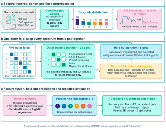
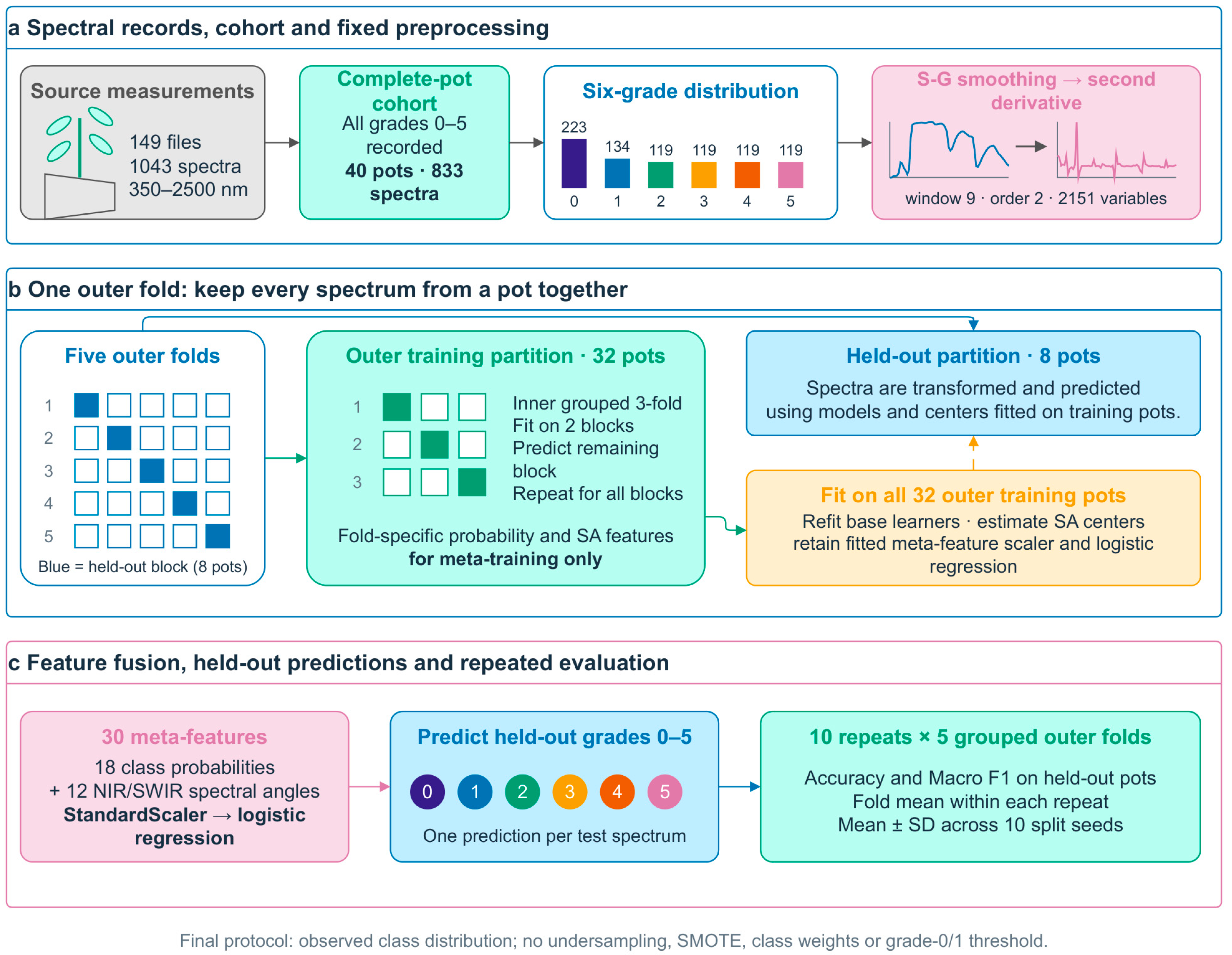
The workflow comprised data acquisition, spectrum-wise preprocessing, grouped model training, and internal evaluation (Figure 1). The primary cohort was defined from recorded pot identifiers before model fitting. Base-learner probabilities and SA features for meta-classifier training were generated within the outer training partition using inner grouped folds. The completed analyses included matched model comparisons, class-level errors, regional SA ablation, repeated evaluation, and local boundary sensitivity.

Figure 1. Workflow of the final no-resampling analysis. Recorded pot groups are separated in the outer five-fold evaluation; three inner grouped folds generate meta-training probabilities and spectral-angle features. The final fusion has 18 probability features and 12 NIR/SWIR spectral-angle features. (a) Spectral record, cohort and fixed preprocessing. (b) One outer fold: keep every spectrum from a pot together. (c) Feature fusion, held-out predictions and repeated evaluation.

2.1.1. Rice Materials and Pathogenicity Assay

Two rice cultivars were used: the blast-resistant near-isogenic line NIL-e1 and the susceptible check Lijiangxintuanheigu (LTH). The collaborating agronomy team confirmed that NIL-e1 is a Pi50-containing near-isogenic line in the LTH background developed by the Plant Protection Research Institute of the Guangdong Academy of Agricultural Sciences. Germinated seeds were sown in 50 pots, each 12.2 cm in diameter, with three planting holes and approximately ten seeds per hole. LTH occupied 40 pots, and NIL-e1 occupied 10 pots. Seedlings were raised under dry cultivation. Starting at the one-leaf-one-heart stage, each pot received 0.5 g of ammonium sulfate on three occasions before inoculation. Plants were spray-inoculated at the 3.5–4-leaf stage. The experiment was conducted at the institute’s experimental base in October 2024.

A well-sporulating isolate was used for inoculation. The collaborating agronomy team confirmed a resistant reaction in NIL-e1 and a susceptible reaction in LTH to this isolate. To activate the isolate and induce sporulation, we cultured it on yeast-solid medium at 25 °C for more than 7 days and then on corn medium for 13 days. Conidia were washed from the corn grains with sterile water. We placed the grains in a sterilized enamel tray under wet gauze and exposed them to fluorescent light for 3–4 days.

Before inoculation, the conidia were washed with sterile water and passed through a double-layer fine mesh to remove corn residue. We adjusted the suspension to approximately 1 × 10⁵ spores/mL and sprayed it evenly over the leaves. The plants stayed for 24 h in a closed, dark chamber at 25 °C and above 95% relative humidity. They were then moved to a glasshouse at 25–28 °C under natural light and maintained until disease symptoms developed. Disease grades and spectra were recorded on days 6–7, when the susceptible check was fully diseased. The collaborating team did not provide a day-by-day record of symptom onset.

2.1.2. Disease Severity Grading

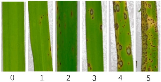
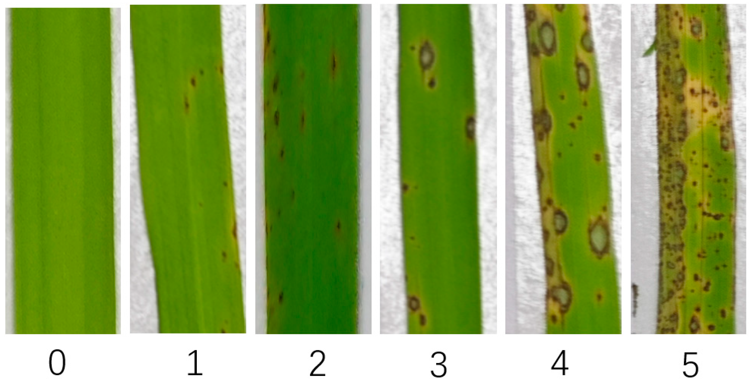
Disease severity was assessed using the grading procedure attributed to the International Rice Research Institute (IRRI) in the original experimental record [20]. The recorded labels comprised six categories, numbered 0–5. Grade 0 denoted no visible symptoms; grade 1, tiny brown specks; grade 2, brown circular spots approximately 1 mm in diameter; grade 3, circular or spindle-shaped lesions 2–3 mm long with gray centers and brown margins; grade 4, spindle-shaped lesions 1–3 mm long with gray centers and brown margins; and grade 5, large, broad, gray spindle-shaped lesions that could coalesce. For the present 0–5 record, grades 0–3 were treated as resistant reactions and grades 4–5 as susceptible reactions. These are visual labels used for classification, not measurements of pathogen load or temporal infection stages. Grade 0 denotes a symptom-free observation and is not, by itself, evidence of a pathogen-negative control. Figure 2 shows representative leaves.

Figure 2. Representative leaf photographs for the six recorded visual severity grades (0–5). These examples illustrate the classification labels; they do not establish pathogen-negative status for grade 0.

2.1.3. Spectral Measurement

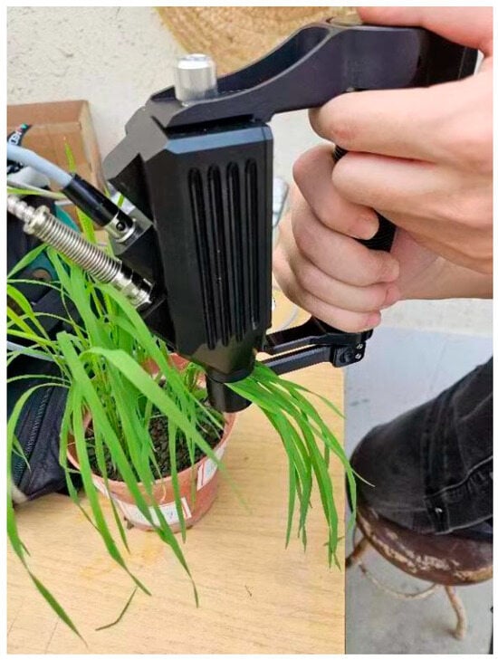
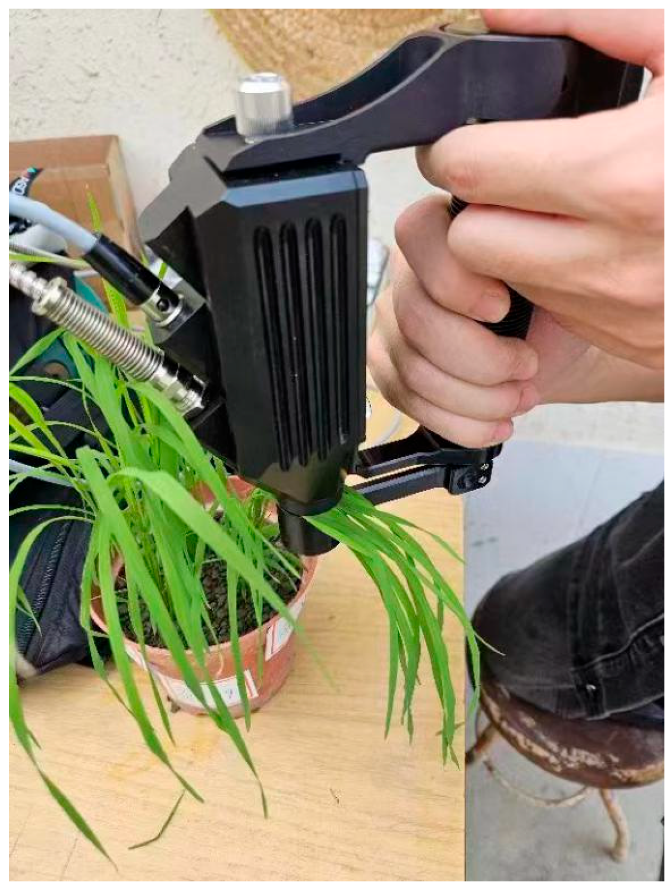
Leaf spectra were collected using an ASD FieldSpec 4 portable spectroradiometer (Analytical Spectral Devices, Inc., Boulder, CO, USA; 350–2500 nm) equipped with a leaf clip. The measurement setup is shown in Figure 3. A leaf clip held the measured leaf area, and a standard white panel was used for instrument calibration before each measurement. The collaborating agronomy team confirmed that the leaf base, middle, and tip were fixed anatomical sampling positions used to sample lesions and adjacent areas consistently, regardless of the exact lesion location. The original protocol describes repeated acquisition on successive days during a stable light window. Records affected by instrument errors or incomplete coverage of that window were excluded. The retained archive contained 1043 spectra across grades 0–5. Each spectrum was a prediction unit, but spectra sharing a recorded pot identifier were treated as dependent observations for data splitting. Figure 3 shows the measurement setup.

Figure 3. Leaf-level spectral acquisition using the ASD FieldSpec 4 spectroradiometer and leaf clip. The acquisition range was 350–2500 nm.

The archive contained 50 distinct recorded pot identifiers. Forty identifiers had observations at all six grades and formed the primary matched cohort of 833 spectra. The grade counts in this cohort were 223, 134, 119, 119, 119, and 119 for grades 0–5, respectively. The collaborating agronomy team confirmed that all six grades occurred in LTH and that the remaining ten grade-0-only pots corresponded to NIL-e1; these ten identifiers were not included in the primary comparison. The team reported no cultivar–grade confounding in the primary cohort. This restriction defines the analysis cohort; it is not random undersampling of grade 0. Table 1 distinguishes spectral counts from the number of recorded pot groups. Further record-level clarifications are included in the Supplementary Materials.

Table 1. Spectral counts and distinct recorded pot identifiers in the archive and primary analysis cohort. Per-grade group counts overlap; the total row gives the number of distinct identifiers, not their sum across grades.

Grade	Archive Spectra	Archive Groups	Primary Spectra	Primary Groups
0	433	50	223	40
1	134	40	134	40
2	119	40	119	40
3	119	40	119	40
4	119	40	119	40
5	119	40	119	40
Total	1043	50	833	40

2.2. Spectral Preprocessing and Analysis Cohort

2.2.1. Savitzky–Golay Smoothing and Second-Derivative Transformation

Each spectrum was first smoothed with a Savitzky–Golay (S–G) filter using a nine-band window and a second-order polynomial. A second S–G operation with the same window and polynomial order produced the second derivative (deriv = 2; delta = 1 band). These spectrum-wise operations do not estimate parameters from other observations. The configuration was retained from model development and applied identically to all models in the final comparison:

$$\overline{R}\left({\lambda }_i\right) = {\sum }_j{c}_{j}R\left({\lambda }_{i+j}\right)$$

(1)

where R(λ_i+j) is the raw reflectance at wavelength λ_i+j, $\overline{\mathrm{R}}\left({\mathsf{\lambda }}_{\mathrm{i}}\right)$ is the smoothed reflectance, and c_j is a smoothing coefficient. The nine-band window has a half-width of four bands.

$$R^{″}\left({\lambda }_i\right) = {\sum }_j{c}_j^{\left(2\right)}\overline{R}\left({\lambda }_{i+j}\right)$$

(2)

where R″(λ_i) is the second-derivative value and c_j⁽²⁾ is the derivative coefficient. The retained wavelength grid contains 2151 bands with a spacing of 1 nm.

2.2.2. Cohort Definition and Class Imbalance

The primary analysis retained every available spectrum from the 40 complete recorded pot groups. No random undersampling, synthetic minority over-sampling technique (SMOTE) [17], Gaussian augmentation, or class weighting was applied in the final protocol. The unequal observed class counts were retained in both training and evaluation.

All spectra associated with a recorded pot identifier were assigned to the same outer fold, including observations from different grades or acquisition dates. The same grouping rule was used in the inner folds for stacking. A pot identifier may occur at multiple grades; therefore, the six per-grade group counts in Table 1 must not be summed as independent biological replicates. The recorded pot identifier was used as the grouping unit for the computational evaluation.

2.3. Model Construction

The matched comparison comprised SVM, RF, XGBoost, XGB-SVM, XGB-SVM-RF, and XGBSVMRF-SA. All base learners used the same 2151-band second-derivative input. The two SA-free stacks supplied probability-fusion controls. Regional SA variants changed only the additional meta-features while sharing base predictions, folds, and meta-classifier settings.

2.3.1. Support Vector Machine (SVM)

SVM estimates a separating boundary by balancing margin width against classification errors [21,22]. We used a radial basis function (RBF) kernel for the nonlinear spectral input:

K(x, z) = exp(−γ‖x − z‖²)

(3)

where γ is the kernel parameter controlling the width of the Gaussian kernel.

2.3.2. Random Forest (RF)

RF fits decision trees to bootstrap samples and considers a random subset of features at each split [23]. In this implementation, class probabilities were averaged across trees. RF supplied a bagging-based probability block alongside the boosting and kernel-based learners. Its incremental predictive contribution was evaluated through matched comparisons.

2.3.3. XGBoost

XGBoost constructs an additive ensemble of decision trees using a regularized objective [24]. The loss term measures prediction error, and the regularization term penalizes model complexity:

$$L = {\sum }_{i}l\left(y_i,{\widehat{y}}_i\right) + {\sum }_k\Omega \left(f_k\right)$$

(4)

where l is the prediction loss and Ω is the regularization term for a tree f_k.

2.3.4. Regional Spectral-Angle (SA) Features

Spectral angle measures the directional similarity of two vectors and provides an explicit descriptor of their relative spectral shape. The ideal nonzero-vector formulation is invariant to positive multiplicative scaling. This property does not extend to additive noise; illumination variability requires separate robustness assessment. Hyperspectral descriptors have been used to characterize disease-associated spectral variation [3,25]. Here, SA was calculated from second-derivative vectors, not directly from raw reflectance. For a preprocessed sample vector x and a grade-center vector c, the angle is:

$$\mathrm{SA}\left(x,c\right) = \arccos \left({\displaystyle \frac{x^{\mathrm{T}}c}{‖x‖‖c‖}}\right)$$

(5)

Candidate regional features were calculated for visible wavelengths (VIS, 350–680 nm), the red edge (680–760 nm), NIR (760–1300 nm), and SWIR (1300–2500 nm). These ranges are conventional spectral partitions rather than experimentally validated physiological optima. The final configuration used NIR and SWIR only for the SA branch; the base learners still received all 2151 bands. The angle for region k is:

$${\mathrm{SA}}_k\left(x_k,c_k\right) = \arccos \left({\displaystyle \frac{{x_k}^{\mathrm{T}}{c}_k}{‖x_k‖‖c_k‖}}\right)$$

(6)

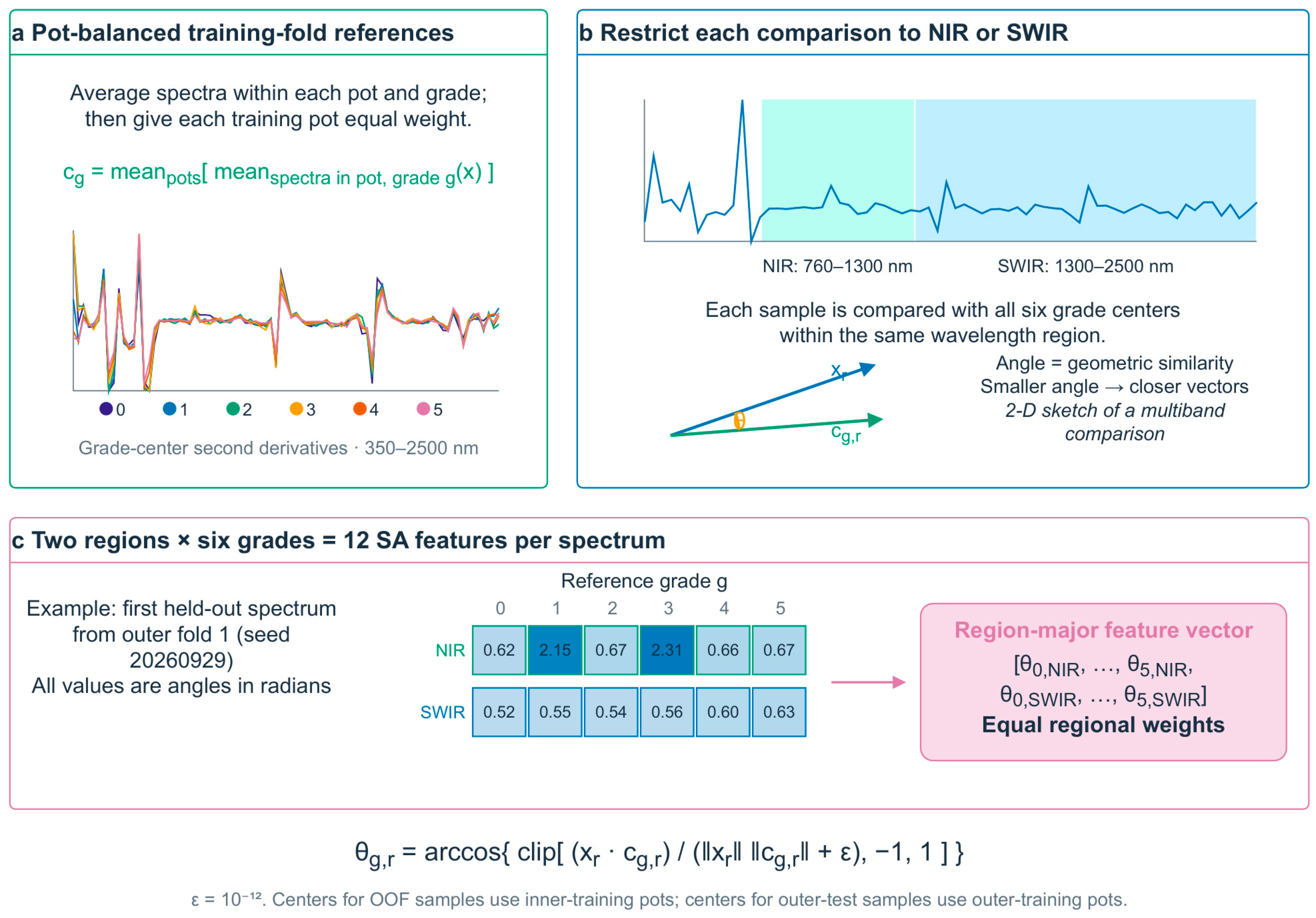
Grade centers were group-balanced: spectra were first averaged within each recorded pot and grade, and then the available pot means were averaged with equal weight. During inner out-of-fold generation, centers were estimated from the inner training groups only; centers for outer-test features were estimated from the complete outer training partition. The implementation adds 10⁻¹² to the norm product and clips the cosine to [−1, 1] before applying arccos. Inclusive wavelength masks are used, so the 1300 nm band is shared by the reference NIR and SWIR ranges. Six grades in two regions yield 12 SA features (Figure 4). No manual regional weights or additional attention layer were used.

Figure 4. Construction of regional spectral-angle features from preprocessed spectra. Group-balanced grade centers are estimated within the relevant training partition. Six comparisons in NIR and six in SWIR yield the 12-dimensional SA branch used by the final model.

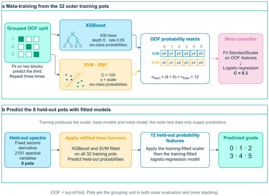
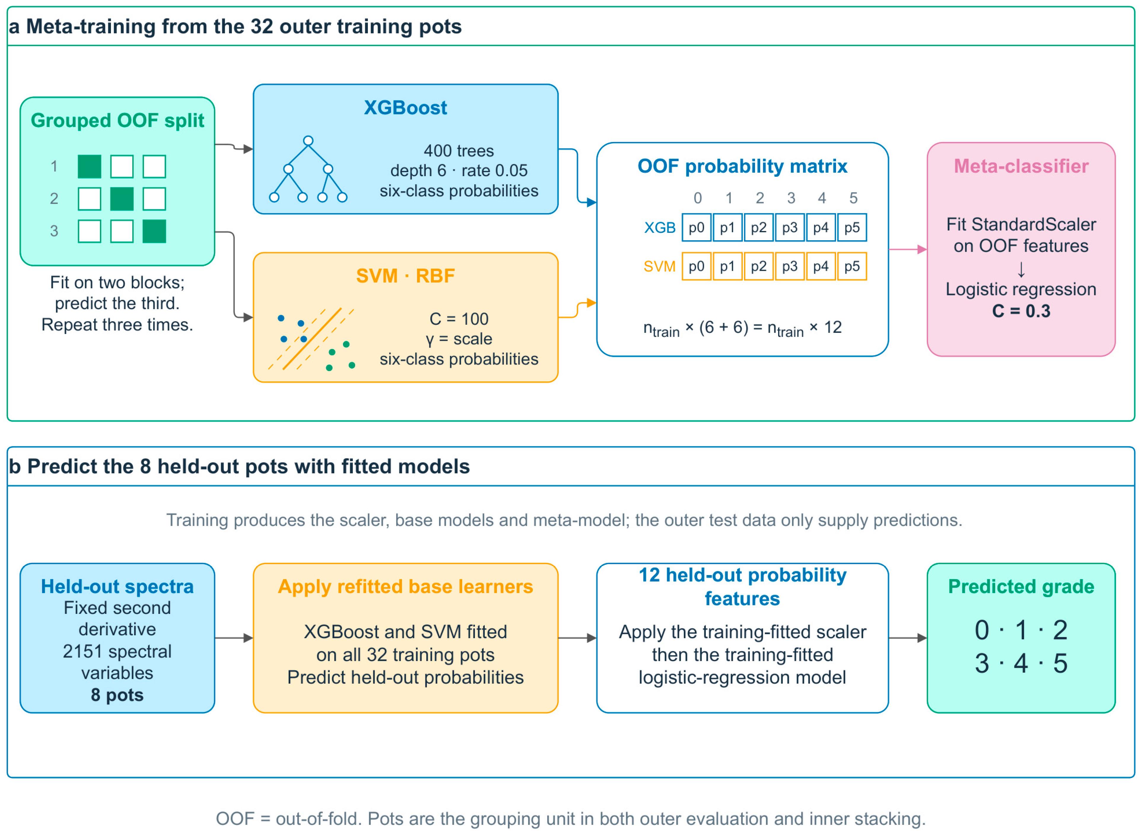
2.3.5. Two-Learner Stacking Model (XGB-SVM)

The XGB-SVM stack combines predictions from XGBoost and SVM through a second-level classifier (Figure 5). Heterogeneous ensemble and feature-fusion approaches provide the broader methodological context [18,26]. Each learner returns a six-class probability vector:

$$P_{\mathrm{XGB}} = \left[p_0^{\mathrm{XGB}}, \dots , p_5^{\mathrm{XGB}}\right], P_{\mathrm{SVM}} = \left[p_0^{\mathrm{SVM}}, \dots , p_5^{\mathrm{SVM}}\right]$$

(7)

Figure 5. Architecture of the SA-free XGB-SVM stack. Two six-class probability blocks form a 12-dimensional input to the standardized logistic-regression meta-classifier; meta-training probabilities are generated out of fold within the outer training data.

Concatenating the two vectors produces a 12-dimensional meta-feature vector z:

z = P_XGB ⊕ P_SVM ∈ ℝ¹²

(8)

Here, ⊕ denotes vector concatenation. Inner grouped out-of-fold predictions provide the meta-training features. After feature standardization, an L2-regularized logistic-regression classifier predicts the final grade:

$$\widehat{y} = {\mathrm{argmax}}_j{\left[\mathrm{LR}\left(z\right)\right]}_j$$

(9)

2.3.6. Heterogeneous Stacking with Regional SA (XGBSVMRF-SA)

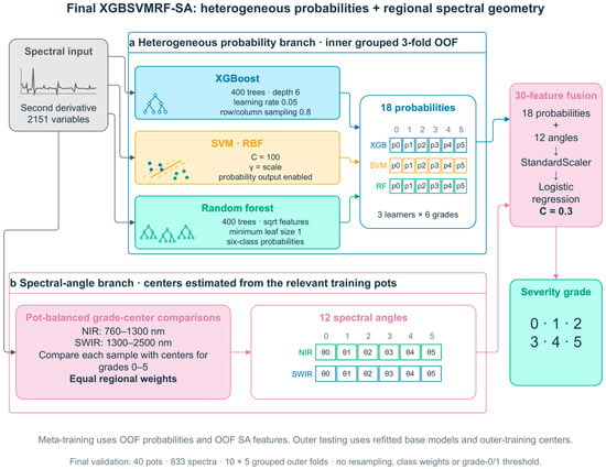
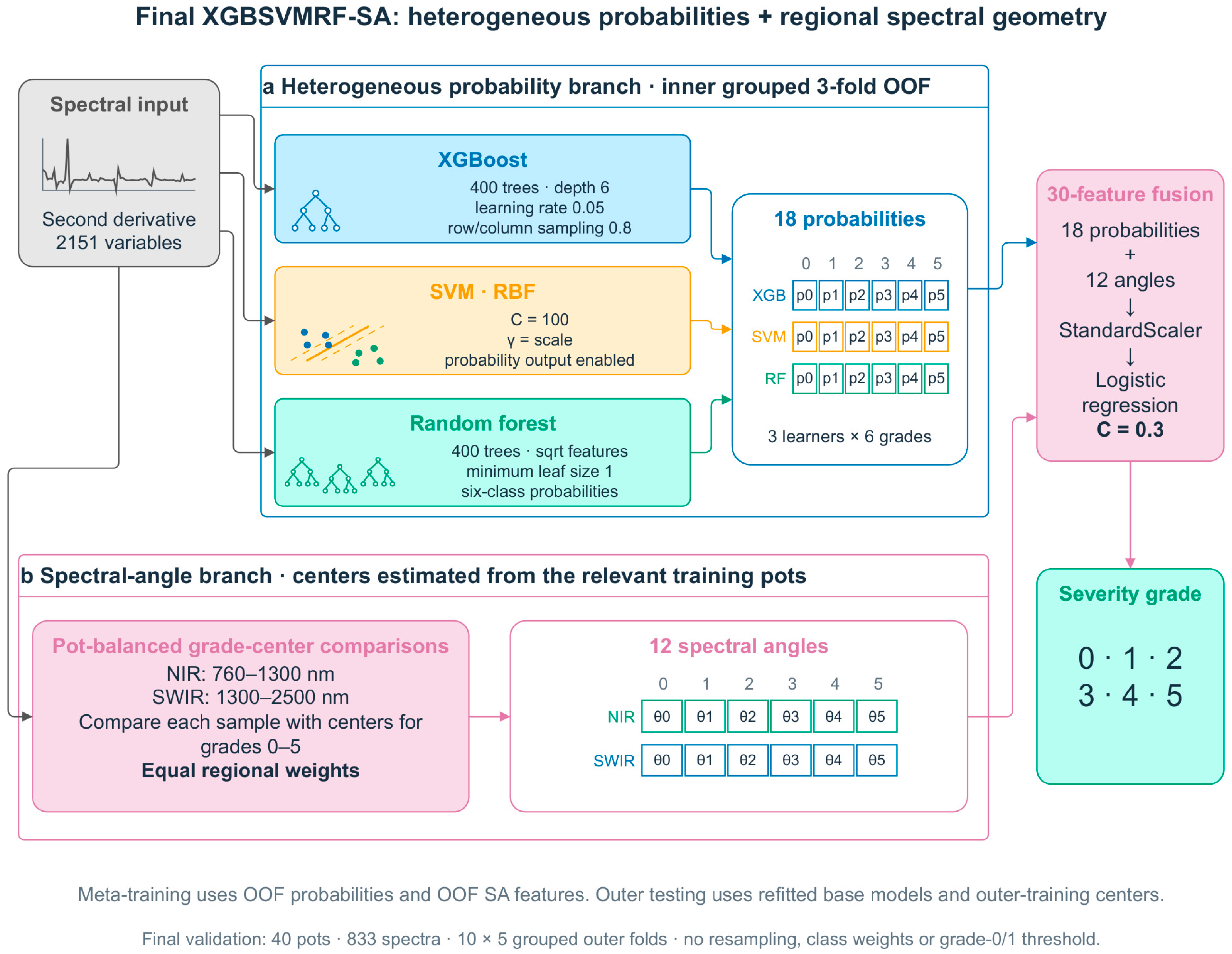
XGBSVMRF-SA extends the SA-free XGB-SVM-RF stack with a regional spectral-angle branch (Figure 6). Its architecture contains a base-learning layer, a geometric feature branch, and a meta-classification layer.

Figure 6. Architecture of XGBSVMRF-SA. The final meta-input concatenates 18 probabilities from XGBoost, SVM, and RF with 12 NIR/SWIR spectral-angle features. The 30-dimensional input is standardized and classified by logistic regression without grade-0/1 threshold adjustment.

The base-learning layer comprises XGBoost, SVM, and RF, representing boosting, kernel-based classification, and bagging, respectively. Each provides probabilities for the same six classes:

P_XGB, P_SVM, P_RF ∈ ℝ⁶

(10)

The SA branch uses Equation (6) to compare a sample with six training-derived grade centers in each of the two retained regions. Its 12 features supply geometric descriptors in addition to the base probabilities. The same inner grouped partitions are used for SA-center estimation and out-of-fold base predictions, so an inner validation group does not contribute to its own reference centers.

The meta-classification layer concatenates the three probability blocks (18 features) and the NIR/SWIR SA vector s (12 features):

F = P_XGB ⊕ P_SVM ⊕ P_RF ⊕ s ∈ ℝ³⁰

(11)

Thus, F is a 30-dimensional vector. Standardization is fitted to the meta-training data only. An L2-regularized logistic-regression classifier produces the class probabilities and assigns the grade with the largest probability:

$$\widehat{y}={\mathrm{argmax}}_j{\left[\mathrm{LR}\left(F\right)\right]}_j$$

(12)

The SA branch augments the meta-classifier with spectral-geometric descriptors while leaving the base-learner objectives unchanged. Its incremental contribution is evaluated against the matched SA-free stack using fold-level, repeated-run, and class-level comparisons.

2.3.7. Model Parameters and Validation Protocol

The principal model comparison used one five-fold StratifiedGroupKFold evaluation with shuffle enabled and random seed 20260929. Recorded pot identifiers defined groups; each outer test fold contained eight of the 40 groups. All analyses were conducted in Python 3.10.11 using scikit-learn 1.7.2, XGBoost 3.1.2, SciPy 1.15.3, NumPy 2.2.6, and pandas 2.3.3. The CUDA-enabled build of XGBoost 3.1.2 was used for XGBoost fitting. Stacking used three-fold StratifiedGroupKFold prediction within each outer training partition. Standardization and grade-center estimation were fitted only to the relevant training data. Base learners were refitted on the full outer training partition to predict its test fold. This grouped internal cross-validation evaluates performance on held-out recorded groups from the study cohort.

XGBoost used 400 trees, learning_rate = 0.05, max_depth = 6, subsample = 0.8, colsample_bytree = 0.8, tree_method = hist, device = cuda, and eval_metric = mlogloss (XGBoost 3.1.2). SVM used an RBF kernel, C = 100, gamma = scale, and probability = True. The base learners received the preprocessed spectra without an additional StandardScaler. RF used 400 trees, max_features = sqrt, and min_samples_leaf = 1. Every stacking comparison used a StandardScaler on its meta-features, followed by logistic regression with C = 0.3, max_iter = 3000, L2 regularization, and no class weights. SVM probability estimation used the internal calibration of SVC, not a custom grouped calibration procedure. The settings of a given base learner were identical across comparisons. No post-hoc decision threshold was used.

For split-stability assessment, the fixed SA-free, all-region SA, and NIR/SWIR SA stacks were evaluated in ten repeated grouped five-fold runs (seeds 20260929–20260938). Within each repeat, the five-fold scores were averaged; the reported mean and standard deviation (SD) were then calculated across the ten repeat means. These ten repeats assess split stability within the same cohort.

Regional comparisons retained the same base predictions and meta-classifier settings. Local sensitivity was evaluated by moving the NIR lower boundary and NIR/SWIR split together by −40, −20, +20, or +40 nm, while fixing the SWIR upper limit at 2500 nm. The reference boundaries were 760 and 1300 nm. Regional choices and model settings were developed using this cohort. These fixed-configuration comparisons therefore provide internal, exploratory evidence. The full selection process was not evaluated in a separate outer validation layer.

2.3.8. Evaluation Metrics

Accuracy is the proportion of correctly classified spectra. Macro F1 is the unweighted mean of the six class-specific F1 scores and gives each grade equal weight despite unequal spectral counts. Primary model and regional tables report the unweighted mean ± sample SD of the five outer fold scores. Class-level metrics and confusion matrices use one pooled out-of-fold prediction per spectrum; these pooled metrics need not equal the unweighted fold means. Precision (P), recall (R), and F1 are defined as:

$$P = {\displaystyle \frac{\mathrm{TP}}{\mathrm{TP} + \mathrm{FP}}}, R = {\displaystyle \frac{\mathrm{TP}}{\mathrm{TP} + \mathrm{FN}}}, {\mathrm{F}}_1 = {\displaystyle \frac{2\mathit{PR}}{P + R}}$$

(13)

TP, FP, and FN denote true positives, false positives, and false negatives for a given class. Percentage-point differences are obtained by subtracting the unrounded metric means before expressing the difference on a 0–100 scale. SD summarizes variability at the stated fold or repeat level. Uncertainty in a new population would require independent validation.

3. Results

3.1. Spectral Profiles and Regional Grade Differences

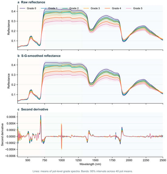
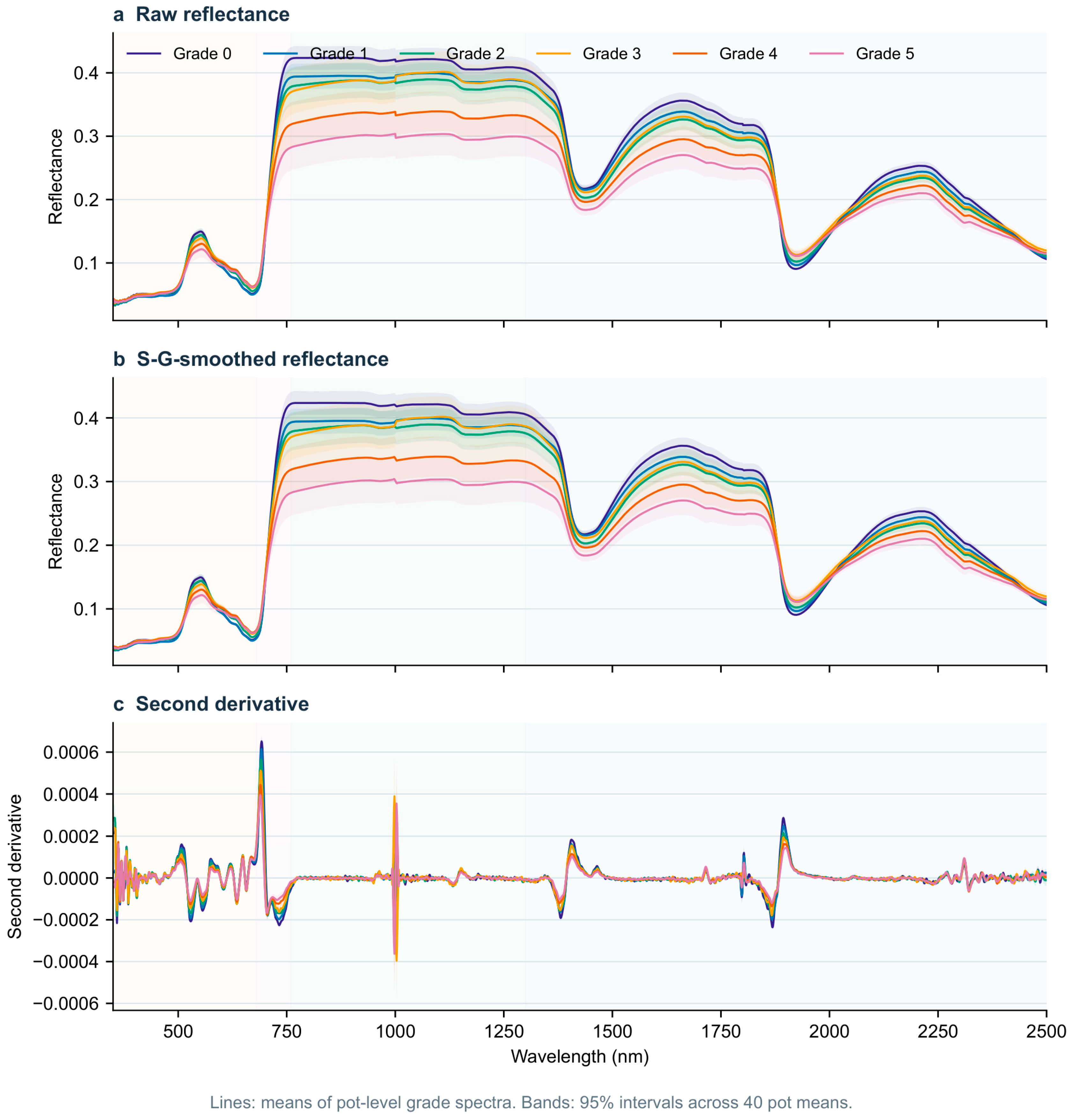
Figure 7 summarizes the grade-wise spectral profiles in the primary cohort. Spectra were averaged within each recorded pot and grade before calculating across-pot summaries. The profiles show overlapping distributions rather than complete grade separation. Friedman tests of pot-level regional mean raw reflectance identified differences among the six recorded grades in VIS (χ² = 17.071, p = 0.00437), the red edge (χ² = 52.114, p = 5.11 × 10⁻¹⁰), NIR (χ² = 70.043, p = 1.00 × 10⁻¹³), and SWIR (χ² = 65.914, p = 7.24 × 10⁻¹³). These are exploratory omnibus comparisons, not tests of SA classification improvement. Their effect sizes and multiplicity context are reported in Table 2.

Figure 7. Grade-wise spectra in the primary cohort: raw reflectance, Savitzky–Golay-smoothed reflectance, and second derivatives. Lines summarize 40 recorded pot means per grade; shaded bands are approximate 95% confidence intervals of the mean (mean ± 1.96 standard errors), not ranges of individual spectra. (a) Raw reflectance (b) S-G-smoothed reflectance (c) Second derivative.

Table 2. Local spectral-boundary sensitivity under the same primary five-fold split. Both the NIR lower limit and NIR/SWIR split move by the indicated amount; 2500 nm remains fixed. Values are five-fold mean ± SD in percent.

Shift (nm)	NIR Range (nm)	SWIR Range (nm)	Accuracy (%)	Macro F1 (%)
−40	720–1260	1260–2500	91.95 ± 2.52	91.33 ± 2.66
−20	740–1280	1280–2500	91.94 ± 2.58	91.32 ± 2.74
0 (ref.)	760–1300	1300–2500	92.07 ± 2.48	91.46 ± 2.63
20	780–1320	1320–2500	92.07 ± 2.48	91.46 ± 2.63
40	800–1340	1340–2500	92.07 ± 2.48	91.46 ± 2.63

3.2. Multi-Model Performance Comparison

Table 3 compares the six models on identical outer folds. Among the individual learners, XGBoost achieved the highest mean accuracy (90.88%) and macro F1 (90.31%), followed by RF (85.46% and 84.66%) and SVM (82.57% and 81.23%). The rankings describe the retained configurations evaluated on this cohort.

Table 3. Matched no-resampling model comparison on 833 spectra from 40 recorded pot groups. Values are percentages and represent the mean ± SD of the same five outer folds (seed 20260929).

Model	Accuracy (%)	Macro F1 (%)
SVM	82.57 ± 1.97	81.23 ± 2.25
RF	85.46 ± 1.85	84.66 ± 2.03
XGBoost	90.88 ± 2.34	90.31 ± 2.58
XGB-SVM	91.34 ± 3.14	90.66 ± 3.36
XGB-SVM-RF	91.34 ± 3.20	90.61 ± 3.45
XGBSVMRF-SA	92.07 ± 2.48	91.46 ± 2.63

The SA-free XGB-SVM stack reached 91.34% accuracy and 90.66% macro F1. XGB-SVM-RF reached 91.34% and 90.61%, respectively. Relative to XGBoost, the three-learner SA-free stack added 0.46 percentage points in accuracy and 0.30 in macro F1. Adding RF to XGB-SVM retained the same rounded accuracy, with a slightly lower mean macro F1 in this comparison.

XGBSVMRF-SA reached 92.07% ± 2.48% accuracy and 91.46% ± 2.63% macro F1. Relative to XGBoost, the complete framework added 1.19 and 1.16 percentage points, respectively. Relative to the matched SA-free XGB-SVM-RF stack, the SA increment was 0.72 percentage points in accuracy and 0.85 in macro F1. This matched evaluation separates the complete-framework gain from the SA-specific increment. Split-stability and paired descriptive analyses are reported separately in Section 3.3.

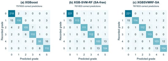
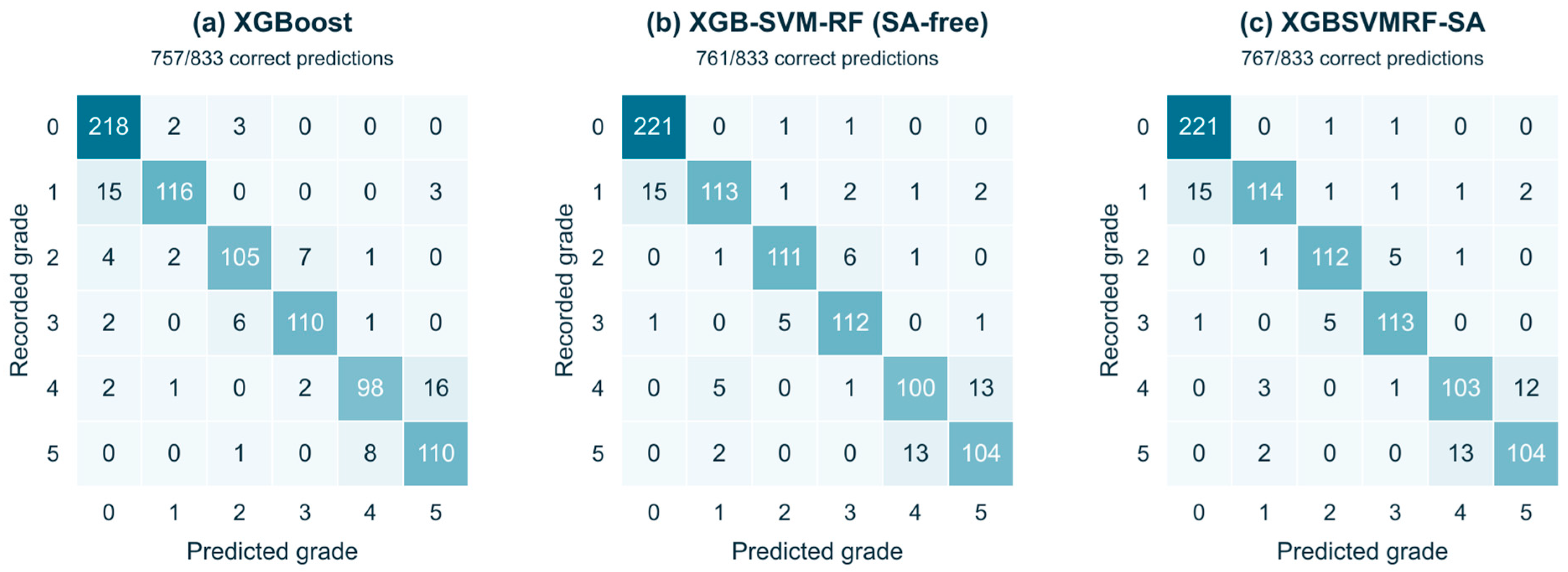
Figure 8 compares the pooled out-of-fold predictions of XGBoost, XGB-SVM-RF, and XGBSVMRF-SA. The numbers of correct predictions were 757, 761, and 767 out of 833, respectively. The SA model yielded six additional correct predictions, with class-specific changes summarized below. Relative to the SA-free stack, the number of correct grade-0 predictions remained 221/223; correct predictions increased from 113 to 114 for grade 1, 111 to 112 for grade 2, 112 to 113 for grade 3, and 100 to 103 for grade 4, while remaining 104 for grade 5. Table 4 reports the complete model’s pooled class metrics. These class-level counts describe the distribution of the observed gain. Detailed fold-by-grade metrics are provided in Supplementary Materials, Table S1.

Figure 8. Pooled confusion matrices for the same 833 spectra under common grouped five-fold evaluation: (a) XGBoost; (b) SA-free XGB-SVM-RF; (c) XGBSVMRF-SA with NIR/SWIR SA. Rows are recorded grades and columns are predictions; no threshold adjustment was used.

Table 4. Pooled out-of-fold class metrics for XGBSVMRF-SA under the common five-fold protocol. Precision, recall, and F1 are percentages. Support is the number of spectra, not the number of independent pots.

Grade	Precision (%)	Recall (%)	F1 (%)	Support
0	93.25	99.10	96.09	223
1	95.00	85.07	89.76	134
2	94.12	94.12	94.12	119
3	93.39	94.96	94.17	119
4	87.29	86.55	86.92	119
5	88.14	87.39	87.76	119
Macro average	91.86	91.20	91.47	833

Table 5 lists the five outer fold scores of the final model. Each test fold contained eight recorded pot groups, with unequal numbers of spectra per fold. The fold SDs were 2.48 percentage points for accuracy and 2.63 for macro F1. These SDs quantify variation across the held-out groups in this split; external generalization is a separate validation question. Table 5 and Table 3 use the same folds and therefore have identical final-model means. Results for the matched SA configurations in each fold are provided in Supplementary Materials Table S2.

Table 5. Fold-level performance of XGBSVMRF-SA in the primary grouped evaluation (seed 20260929). Metrics are percentages; each fold holds out eight recorded pot groups.

Fold	Test spectra	Accuracy (%)	Macro F1 (%)
1	161	90.68	90.06
2	168	89.29	88.44
3	168	91.67	91.27
4	168	95.83	95.50
5	168	92.86	92.04
Mean ± SD	—	92.07 ± 2.48	91.46 ± 2.63

3.3. Regional SA Ablation and Repeated Evaluation

Table 6 compares regional SA feature sets while holding base predictions and meta-classifier settings fixed. NIR/SWIR SA produced the highest numerical fold-mean macro F1 (91.46%), followed by SWIR-only SA (91.06%), VIS-only SA (90.97%), all-region SA (90.95%), red-edge-only SA (90.74%), and NIR-only SA (90.60%). The SA-free reference reached 90.61%. The combined NIR/SWIR descriptor offered the strongest numerical result among the tested regional configurations. This supports its use in the present model and motivates task-specific evaluation of alternative wavelength ranges.

Table 6. Regional SA comparisons with matched base predictions and meta-classifier settings. Values are five-fold mean ± SD in percent. All-region SA uses 24 angle features; the final NIR/SWIR branch uses 12, and each single-region branch uses six.

SA Feature Set	Accuracy (%)	Macro F1 (%)
SA-free	91.34 ± 3.20	90.61 ± 3.45
VIS	91.71 ± 2.36	90.97 ± 2.49
Red-edge	91.45 ± 3.36	90.74 ± 3.63
NIR	91.34 ± 3.14	90.60 ± 3.41
SWIR	91.71 ± 2.25	91.06 ± 2.36
All-region	91.58 ± 2.13	90.95 ± 2.34
NIR+SWIR	92.07 ± 2.48	91.46 ± 2.63

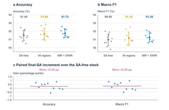
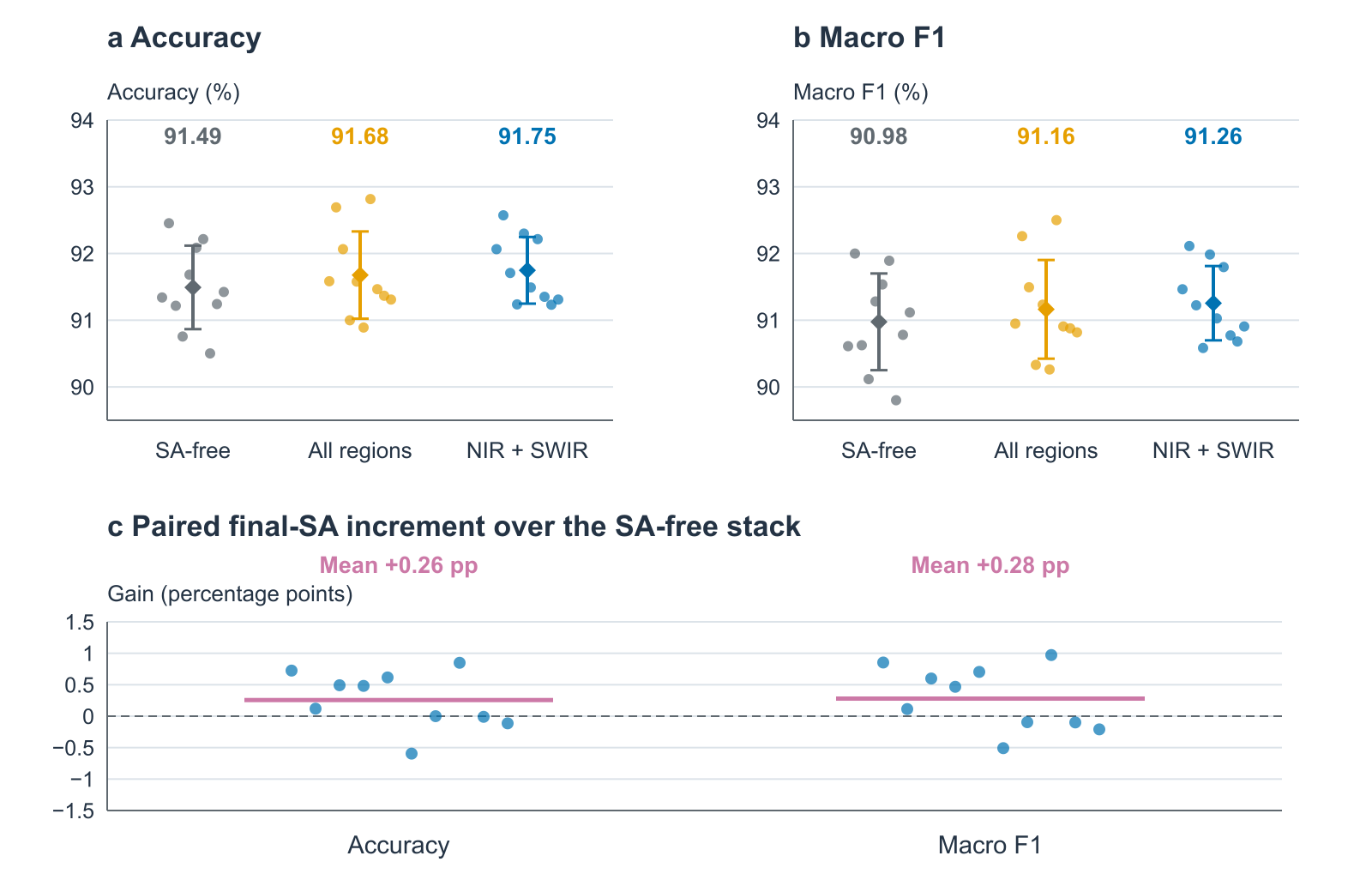
Table 7 and Figure 9 summarize ten repeated grouped five-fold runs. XGBSVMRF-SA achieved 91.75% ± 0.50% accuracy and 91.26% ± 0.56% macro F1, compared with 91.49% ± 0.63% and 90.98% ± 0.72% for the SA-free stack. The mean paired increments were 0.26 and 0.28 percentage points. SA gave higher accuracy in six repeats, tied in one, and was lower in three; macro F1 was higher in six and lower in four. The repeat-wise differences and SDs summarize split stability within the same cohort. Ten-repeat summaries for the SA configurations are provided in Supplementary Materials, Table S3; repeated class-specific results are given in Table S4.

Table 7. Fixed-configuration performance in ten repeated pot-grouped five-fold runs. Values are percentages and summarize the ten within-repeat fold means (mean ± SD across repeat means), not 50 independent fold experiments.

Fixed Configuration	Accuracy (%)	Macro F1 (%)
XGB-SVM-RF (SA-free)	91.49 ± 0.63	90.98 ± 0.72
All-region SA	91.68 ± 0.65	91.16 ± 0.74
XGBSVMRF-SA (NIR/SWIR)	91.75 ± 0.50	91.26 ± 0.56

Figure 9. Ten repeated grouped five-fold evaluations. In panels (a,b), dots are within-repeat fold means, diamonds are across-repeat means, and bars are SD across ten repeat means; scores are percentages. Panel (c) shows paired SA increments in percentage points.

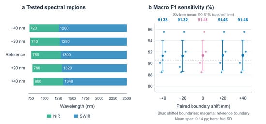
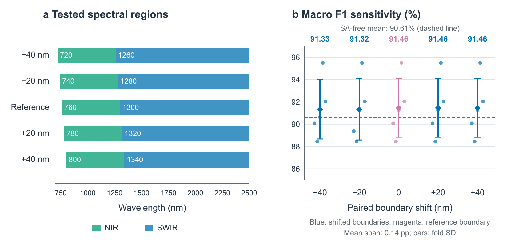
The boundary experiment (Table 2 and Figure 10) shifted the two NIR-related boundaries together while keeping the SWIR endpoint and model settings fixed. Across the five tested definitions, mean accuracy ranged from 91.94% to 92.07%, and mean macro F1 ranged from 91.32% to 91.46%. The macro F1 span was 0.14 percentage points. Positive shifts of 20 and 40 nm produced the same predicted-label scores as the reference. The narrow score range suggests limited sensitivity to these local boundary shifts within the tested configuration.

Figure 10. Local NIR/SWIR boundary sensitivity: (a) tested wavelength ranges and (b) macro F1 in percent. Dots are individual fold scores; diamonds and bars are the mean ± SD of the same five folds. The two NIR-related boundaries shift together, while the SWIR upper limit remains 2500 nm.

3.4. Exploratory Regional Reflectance Comparisons

Table 8 summarizes the exploratory Friedman tests of regional mean reflectance across grades.

Table 8. Exploratory Friedman comparisons of regional mean raw reflectance among grades, using 40 recorded pot identifiers as paired blocks. The p-values are unadjusted omnibus results for four regional tests; Kendall W is an effect-size measure, not a model-performance metric.

Region	Friedman χ2	df	Unadjusted p	Kendall W
VIS	17.071	5	0.00437	0.085
Red edge	52.114	5	5.11 × 10−10	0.261
NIR	70.043	5	1.00 × 10−13	0.350
SWIR	65.914	5	7.24 × 10−13	0.330

Each Friedman test used five degrees of freedom. NIR and SWIR had the largest regional Kendall W values (0.350 and 0.330). The omnibus tests characterize grade-associated regional differences. Pair-specific contrasts and model gains address separate questions. Separate exploratory wavelength comparisons used Benjamini–Hochberg adjustment across 2151 wavelengths, and adjacent-grade regional comparisons used Holm adjustment within the five contrasts of each region; these exploratory descriptions of spectral variation are distinct from the matched evaluation of the classification gain.

Table 8. Exploratory Friedman comparisons of regional mean raw reflectance among grades, using 40 recorded pot identifiers as paired blocks. The p-values are unadjusted omnibus results for four regional tests; Kendall W is an effect-size measure, not a model-performance metric.

Region	Friedman χ2	df	Unadjusted p	Kendall W
VIS	17.071	5	0.00437	0.085
Red edge	52.114	5	5.11 × 10−10	0.261
NIR	70.043	5	1.00 × 10−13	0.350
SWIR	65.914	5	7.24 × 10−13	0.330

Each Friedman test used five degrees of freedom. NIR and SWIR had the largest regional Kendall W values (0.350 and 0.330). The omnibus tests characterize grade-associated regional differences. Pair-specific contrasts and model gains address separate questions. Separate exploratory wavelength comparisons used Benjamini–Hochberg adjustment across 2151 wavelengths, and adjacent-grade regional comparisons used Holm adjustment within the five contrasts of each region; these exploratory descriptions of spectral variation are distinct from the matched evaluation of the classification gain.

4. Discussion

4.1. Heterogeneous Stacking and Regional Spectral Geometry

The matched comparison separates the gain of the complete framework from that of its individual components. The SA-free three-learner stack was slightly higher than XGBoost, and regional SA added a further numerical gain in the principal five-fold evaluation. Repeated evaluations yielded a smaller, positive mean increment, suggesting a supplementary predictive contribution from SA; the paired comparison is reported in Section 3. The methodological contribution is the use of spectral-geometric descriptors alongside heterogeneous class probabilities. Regional ablation favors a targeted descriptor rather than simply increasing the feature count. Feature selection remains task-dependent, as illustrated by prior spectral-band studies [27]. The base learners used all 2151 bands; reduced-band alternatives are a useful direction for matched evaluation.

4.2. Relationship to Prior Work

Heterogeneous ensemble learning and spectral-feature fusion are established approaches [18,26]. Our contribution is their specific integration with training-derived regional grade-center angles and a pot-grouped evaluation for six recorded visual grades. Related studies address rice leaf-blast detection using UAV measurements [28] and reflectance-based wheat disease assessment [19]. Cross-study comparisons are therefore organized by task, acquisition scale, cohort composition, and validation design, with published accuracies interpreted in their respective settings. A study-by-study comparison is provided in Supplementary Materials, Table S5.

Zou et al. [18] studied stacked ensemble learning and hyperspectral feature fusion for seed classification and mildew detection. The extension in XGBSVMRF-SA is an explicit regional spectral-geometric input to the probability-fusion stack. Rice reflectance and SPAD studies [29] provide context for spectral sensitivity to plant condition, but the present measurements do not establish causal links between particular SA features and pigments, water content, or tissue structure. The regional reflectance tests show association with recorded grades, not validation of an SA mechanism.

4.3. Sources of Confusion Between Adjacent Grades

In the pooled predictions of the complete model, 53 of 66 errors occurred between adjacent grades. The 4/5 pair accounted for 25 errors and the 0/1 pair for 15; these counts summarize the pooled prediction pattern. Grade 0 had a pooled F1 of 96.09%, whereas grades 4 and 5 had F1 values of 86.92% and 87.76%. The grade-0 true-positive count remained unchanged relative to the SA-free stack, so a specific grade-0/1 separation benefit requires further evidence.

Spectral overlap, uncertainty in visual labels, and dependence on acquisition date or plant identity are possible explanations for residual errors. Physiological saturation is a hypothesis, not a measured cause in this dataset. Temporal spectral measurements and image-based methods have been investigated in related work [30,31], but their added value was not tested in the final matched comparison. Future evaluation should distinguish adjacent-category prediction from presymptomatic diagnosis, which was not evaluated in the present analysis.

4.4. Study Scope and Future Validation

The grouped analyses define a methodological contribution under the recorded acquisition conditions. Further evaluation can build on this framework by clarifying experimental-unit metadata, assessing model selection, and testing transfer to independent settings.

First, the cohort comes from one controlled experiment. The collaborating agronomy team confirmed that all six grades occurred in LTH, that the ten grade-0-only pots belonged to NIL-e1, and that cultivar was not confounded with grade in the primary analysis cohort. The analysis uses the recorded identifiers available in the spectral archive as the grouping unit. Pot-grouped splitting reduces overlap associated with the recorded identifiers; it does not remove possible date–grade dependence or demonstrate transfer to another cultivar. Effects of location, season, growth stage, and field conditions remain untested [32].

Second, method development and internal evaluation used the same cohort, so the ten repeated runs assess split stability within those observations. The evaluation used neither an independent external cohort nor fully nested selection of all hyperparameter and regional choices. The positive mean SA increment is interpreted as a numerical contribution under the tested protocol. Third, local boundary perturbations characterize a specified neighborhood of the retained regions; evaluating a broader search requires a separate protocol.

Thirdly, the final SA branch includes SWIR, and the base learners still use the full 350–2500 nm spectrum. Replacing the instrument with a VIS/NIR-only or reduced-band sensor would therefore require a separate matched evaluation. Regional ablation provides an empirical view of the added SA inputs. SHAP, LIME, and independent physiological validation were not part of the completed analyses and are reserved for future interpretation. Independent field cohorts, verified experimental-unit metadata, and transparent access to data and code would extend the present methodological assessment toward practical deployment.

5. Conclusions

XGBSVMRF-SA integrates heterogeneous probability fusion with regional spectral-angle descriptors for six recorded severity grades. Its 30-dimensional meta-input combines 18 class probabilities with 12 NIR/SWIR angles, without resampling or threshold adjustment. In the common grouped five-fold evaluation, accuracy was 92.07% and macro F1 was 91.46%, exceeding XGBoost by 1.19 and 1.16 percentage points, respectively. SA added 0.72 and 0.85 percentage points over the matched SA-free stack in that split. Across ten repeated evaluations, the mean SA increments were positive at 0.26 and 0.28 percentage points. The tested local boundary shifts produced small score variations. Regional SA supplies a supplementary spectral-geometric input alongside class probabilities, offering a feature-integration approach for heterogeneous stacking. These findings provide a basis for independent validation and further model development in quantitative severity grading.

References

- Wang, X.; Li, J.; Li, J.; Chen, Y.; Shi, J.; Liu, J.; Sriboonchitta, S. Temporal and spatial evolution of rice productivity and its influencing factors in China. Agronomy 2023, 13, 1075. [Google Scholar] [CrossRef] [Scilit]
- Dean, R.; Van Kan, J.A.L.; Pretorius, Z.A.; Hammond-Kosack, K.E.; Di Pietro, A.; Spanu, P.D.; Rudd, J.J.; Dickman, M.; Kahmann, R.; Ellis, J.; et al. The top 10 fungal pathogens in molecular plant pathology. Mol. Plant Pathol. 2012, 13, 414–430. [Google Scholar] [CrossRef] [Scilit]
- Mandal, N.; Adak, S.; Das, D.K.; Sahoo, R.N.; Mukherjee, J.; Kumar, A.; Chinnusamy, V.; Das, B.; Mukhopadhyay, A.; Rajashekara, H.; et al. Spectral characterization and severity assessment of rice blast disease using univariate and multivariate models. Front. Plant Sci. 2023, 14, 1067189. [Google Scholar] [CrossRef] [Scilit]
- Maina, A.W.; Oerke, E.C. Characterization of rice–Magnaporthe oryzae interactions by hyperspectral imaging. Plant Dis. 2023, 107, 3412–3421. [Google Scholar] [CrossRef] [Scilit]
- Mahlein, A.K. Plant disease detection by imaging sensors—Parallels and specific demands for precision agriculture and plant phenotyping. Plant Dis. 2016, 100, 241–251. [Google Scholar] [CrossRef] [Scilit]
- Shi, J.J.; Liu, Z.Q.; Zhang, L.; Zhou, T.; Huang, J.F. Hyperspectral recognition of rice damaged by rice leaf roller based on support vector machine. Chin. J. Rice Sci. 2009, 23, 331–334. Available online: http://www.ricesci.cn/CN/Y2009/V23/I3/331 (accessed on 7 October 2026). (In Chinese)
- Huang, S.P.; Qi, L.; Ma, X.; Xue, K.; Wang, W. Grading method of rice panicle blast severity based on hyperspectral imaging. Trans. Chin. Soc. Agric. Eng. 2015, 31, 212–219. (In Chinese) [Google Scholar] [CrossRef]
- Zhang, G.S.; Xu, T.Y.; Tian, Y.W.; Feng, S.; Zhao, D.; Guo, Z. Classification of rice leaf blast severity using hyperspectral imaging. Sci. Rep. 2022, 12, 19757. [Google Scholar] [CrossRef] [Scilit]
- Zhang, G.S.; Xu, T.Y.; Tian, Y. Hyperspectral imaging-based classification of rice leaf blast severity over multiple growth stages. Plant Methods 2022, 18, 123. [Google Scholar] [CrossRef] [Scilit]
- Mei, G.Y.; Li, R.; Mei, X.; Chen, R.Q.; Fan, Y.G.; Cheng, J.P.; Feng, Z.; Tao, T.; Zhao, Q.; Zhao, P.; et al. Hyperspectral disease index estimation model for wheat stripe rust based on VSURF-CA. Sci. Agric. Sin. 2024, 57, 484–499. (In Chinese) [Google Scholar] [CrossRef]
- Luo, Z.S.; Liu, Y.C.; Wang, X.D.; Zhang, Q.J. Early identification of potato late blight using hyperspectral imaging combined with BiTCN-SA. J. Shandong Agric. Univ. (Nat. Sci. Ed.) 2026, 57, 56–65. (In Chinese) [Google Scholar] [CrossRef]
- Nguyen, D.H.D.; Tan, A.J.H.; Lee, S. Monitoring of plant diseases caused by Fusarium commune and Rhizoctonia solani in bok choy using hyperspectral remote sensing and machine learning. Pest Manag. Sci. 2024, 80, 4562–4571. [Google Scholar] [CrossRef] [Scilit]
- Deng, X.L.; Zeng, G.L.; Zhu, Z.H.; Huang, Z.X.; Yang, J.C.; Tong, Z.J.; Yin, X.B.; Wang, T.W.; Lan, Y.B. Classification of diseased citrus plants and characteristic band extraction based on UAV hyperspectral remote sensing. J. South China Agric. Univ. 2020, 41, 100–108. [Google Scholar] [CrossRef]
- Li, G.M.; Zhao, D.X.; Li, J.P.; Feng, S.; Chen, C. Unmanned aerial vehicle hierarchical detection of leaf blast in rice crops based on a specific spectral vegetation index. Front. Agric. Sci. Eng. 2025, 12, 211–222. [Google Scholar] [CrossRef] [Scilit]
- Yuan, J.Q.; Qiu, X.C.; Jia, Y.J.; Nan, Y.; Su, Z. Early identification of rice panicle blast in canopy based on hyperspectral imaging. J. Southwest Univ. (Nat. Sci. Ed.) 2023, 45, 57–65. (In Chinese) [Google Scholar] [CrossRef]
- Lü, G.Q.; Yilimunuer, W.; Shan, D.D.; Sun, W.H.; Mao, H.P.; Song, J.X. Spectral characteristics and incubation-period diagnosis technology of rice blast disease based on FTIR-PAS. Trans. Chin. Soc. Agric. Eng. 2025, 41, 163–172. (In Chinese) [Google Scholar] [CrossRef]
- Chawla, N.V.; Bowyer, K.W.; Hall, L.O.; Kegelmeyer, W.P. SMOTE: Synthetic minority over-sampling technique. J. Artif. Intell. Res. 2002, 16, 321–357. [Google Scholar] [CrossRef] [Scilit]
- Zou, Z.; Zhen, J.; Wang, Q.; Wu, Q.; Li, M.; Yuan, D.; Cui, Q.; Zhou, M.; Xu, L. Research on nondestructive detection of sweet-waxy corn seed varieties and mildew based on stacked ensemble learning and hyperspectral feature fusion technology. Spectrochim. Acta Part A Mol. Biomol. Spectrosc. 2024, 320, 124816. [Google Scholar] [CrossRef] [Scilit]
- Cross, J.F.; Cobo, N.; Drewry, D.T. Non-invasive diagnosis of wheat stripe rust progression using hyperspectral reflectance. Front. Plant Sci. 2024, 15, 1429879. [Google Scholar] [CrossRef] [Scilit]
- International Rice Research Institute (IRRI). Standard Evaluation System for Rice, 4th ed.; IRRI: Los Baños, Philippines, 1996. [Google Scholar]
- Vapnik, V.N. The Nature of Statistical Learning Theory; Springer: New York, NY, USA, 1995. [Google Scholar]
- Cortes, C.; Vapnik, V. Support vector networks. Mach. Learn. 1995, 20, 273–297. [Google Scholar] [CrossRef] [Scilit]
- Breiman, L. Random forests. Mach. Learn. 2001, 45, 5–32. [Google Scholar] [CrossRef] [Scilit]
- Chen, T.Q.; Guestrin, C. XGBoost: A scalable tree boosting system. In Proceedings of the 22nd ACM SIGKDD International Conference on Knowledge Discovery and Data Mining; ACM: New York, NY, USA, 2016; pp. 785–794. [Google Scholar]
- Mahlein, A.K.; Steiner, U.; Hillnhütter, C.; Dehne, H.W.; Oerke, E.C. Hyperspectral imaging for small-scale analysis of symptoms caused by different sugar beet diseases. Plant Methods 2012, 8, 3. [Google Scholar] [CrossRef] [Scilit]
- Huang, L.S.; Liu, Y.; Huang, W.J.; Dong, Y.; Ma, H.; Wu, K.; Guo, A. Combining random forest and XGBoost methods in detecting early and mid-term winter wheat stripe rust using canopy level hyperspectral measurements. Agriculture 2022, 12, 74. [Google Scholar] [CrossRef] [Scilit]
- Gu, L.X.; Fang, T.; Du, L.D.; Wu, X.F.; Li, C.C.; Lian, Z.Z.; Yue, Z. Feature band selection and construction of monitoring model of wheat stripe rust based on CA/SPA-CARS algorithm. Trans. Chin. Soc. Agric. Mach. 2025, 56, 487–498. (In Chinese) [Google Scholar] [CrossRef]
- Zhao, D.; Cao, Y.; Li, J.; Cao, Q.; Li, J.; Guo, F.; Feng, S.; Xu, T. Early detection of rice leaf blast disease using UAV remote sensing: A novel approach integrating a new spectral vegetation index and machine learning. Agronomy 2024, 14, 602. [Google Scholar] [CrossRef] [Scilit]
- Wang, A.; Song, Z.; Xie, Y.; Hu, J.; Zhang, L.; Zhu, Q. Detection of rice leaf SPAD and blast disease using integrated aerial and ground multiscale canopy reflectance spectroscopy. Agriculture 2024, 14, 1471. [Google Scholar] [CrossRef] [Scilit]
- Wang, W.; Zhang, Y.; Huang, H.; Liu, T.; Zeng, M.; Fu, Y.; Shu, H.; Yang, J.; Yu, L. Monitoring rice blast disease progression through the fusion of time-series hyperspectral imaging and deep learning. Agronomy 2026, 16, 136. [Google Scholar] [CrossRef] [Scilit]
- Fedotov, A.; Eremenko, D.; Kuznetsova, D.; Baranova, O.; Terentev, A. Advanced hyperspectral image processing and machine learning approaches for early detection of wheat stem rust. Front. Plant Sci. 2025, 16, 1725017. [Google Scholar] [CrossRef] [Scilit]
- Xue, B.; Kong, Y.Y.; Zarco-Tejada, P.J.; Tian, L.; Poblete, T.; Wang, X.; Zheng, H.; Jiang, C.; Yao, X.; Zhu, Y.; et al. Mitigating the phenological influence on spectroscopic quantification of rice blast disease severity with extended PROSAIL simulations. Remote Sens. Environ. 2026, 332, 115063. [Google Scholar] [CrossRef] [Scilit]
Disclaimer/Publisher’s Note: The statements, opinions and data contained in all publications are solely those of the individual author(s) and contributor(s) and not of MDPI and/or the editor(s). MDPI and/or the editor(s) disclaim responsibility for any injury to people or property resulting from any ideas, methods, instructions or products referred to in the content. |
© 2026 by the authors. Licensee MDPI, Basel, Switzerland. This article is an open access article distributed under the terms and conditions of the Creative Commons Attribution (CC BY) license.