


Abstract
Controlling the microclimate in pig housing is essential for ensuring animal welfare and optimizing production efficiency. However, the dynamic, non-linear interactions of environmental and animal variables make microclimate management a complex undertaking. To better understand these interactions and develop predictive models to improve microclimate conditions in swine housing, in this study we analyzed indoor and outdoor temperature, CO2 concentration, and animal activity in a naturally ventilated pig-fattening house using wavelet analysis, cosine models and coherence analysis. The wavelet analysis identified dominant periods of 24 and 12 h for temperatures, along with a relevant contribution from animal activity for the 8 h period. CO2 concentration showed no persistent oscillatory pattern during the production cycle. The three harmonic cosine models provided satisfactory results for outdoor temperature (RMSE = 0.09–0.10; R2 = 0.65–0.84), indoor temperature (RMSE = 0.08–0.10; R2 = 0.52–0.78) and animal activity (RMSE = 0.06–0.16; R2 = 0.43–0.61), but they were not suitable for CO2 modelling. The wavelet coherence analysis revealed temporal phase differences among variables, notably with outdoor temperature and animal activity leading indoor temperature.
1. Introduction
The intensification of livestock farming, added to increasing social and economic pressure to improve animal welfare and reduce environmental impact, is driving change in livestock farm management [1]. In this context, controlling the indoor microclimate is fundamental to animal welfare and production efficiency [2,3,4]. However, such control presents significant complexity as it involves multiple interacting animal and environmental variables such as indoor and outdoor temperature, carbon dioxide (CO2) concentration and animal activity in a dynamic, non-linear system with marked temporal variability. Because each variable is conditioned by numerous factors, precise regulation of indoor environmental conditions in livestock facilities has proven challenging [5]. Understanding how variables interact with each other is therefore essential to developing precision livestock farming (PLF) systems capable of optimizing indoor climate control and reducing greenhouse gas emissions [6,7].
Climate control system performance is equally crucial when it comes to safeguarding animal health and welfare in modern intensive pig production systems, where respiratory diseases constitute the main health problem [3]. These pathologies are closely linked to air quality, temperature and humidity, which directly influence animal welfare, health and productivity [8,9,10]. Restrictions on antibiotic use are also leading producers to adopt new strategies based on biosecurity, management and animal welfare [11,12].
Pigs are especially sensitive to the conditions of their housing environment, and maintaining a thermoneutral environment is essential to well-being. It prevents them from using energy to regulate their temperature, to the detriment of growth and productivity. Some authors have observed that, outside certain thermal thresholds, finishing pigs present physiological alterations and reduced feed and water consumption, which negatively affects production [2,13,14,15,16,17]. However, other authors [18] observed no impact on growth performance. Such research discrepancies point to a need for further study of how heat stress impacts finishing pigs [19].
Carbon dioxide levels are a primary indicator of air quality in intensive pig production facilities [20]. CO2 mainly derives from animal respiration [21] and varies according to physiological stage, body mass, feed intake, and activity level [22,23]. Degradation of organic matter in animal waste slurry also produces CO2, although to a lesser degree [24,25,26].
Activity is another important indicator of animal welfare, as it reveals behavioural changes associated with environmental issues or handling [27,28]. Several studies have identified the close relationship between animal activity and microclimatic variables such as temperature and CO2 concentration [29,30]. While some authors describe a negative correlation between CO2 emissions and activity [31], others have found that CO2 concentrations increased during periods of increased metabolic activity, such as feeding or stress [32]. High concentrations of gases and excessive temperatures also reduce animal activity, causing them to favour resting behaviours and implement strategies to dissipate heat, such as lying on the ground or avoiding contact with other individuals [2,5,29,33,34].
In northwestern Spain, pig-fattening buildings are predominantly naturally ventilated due to the prevailing Atlantic climatic conditions. However, natural ventilation may become insufficient under certain environmental conditions, leading to the accumulation of heat, humidity and gases that deteriorate indoor air quality [35], negatively affecting animal welfare and production. Animal activity, indoor and outdoor temperatures, and CO2 concentration are dynamically interrelated, jointly shaping the environmental conditions within livestock buildings. Besides their contribution as greenhouse gases, elevated CO2 concentrations have been associated with reduced animal welfare and growth performance, and are widely considered an indicator of ventilation effectiveness in livestock buildings. Variations in animal activity directly influence heat production and CO2 concentration [20,36]. In turn, inadequate environmental conditions, including elevated CO2 concentrations, may compromise animal welfare and, in extreme situations, animal survival [21,35,37,38]. Consequently, monitoring and modelling CO2 concentration is particularly relevant for improving environmental control in naturally ventilated pig houses. In this context, outdoor temperature acts as one of the main drivers of indoor environmental dynamics [5], conditioning both indoor temperature and CO2 concentration, which have been reported to be inversely related to animal activity [7].
Optimizing pig-housing microclimates requires an integrated approach that involves continuous monitoring of environmental and animal variables to account for air quality, physiological needs, animal welfare, management and housing characteristics. Various mathematical and computational approaches have been developed to predict the behaviour of these complex and dynamic systems, including machine-learning techniques [39,40,41,42], deep learning [9,10,43], neural networks [5,44,45,46], wavelet neural networks [25,30,47], hybrid models [6,17,48,49] and statistical regression or ARIMA models [50,51]. Other tools, such as the continuous wavelet transform and the coherence wavelet, have also facilitated the analysis of periodicities and temporal relationships among environmental variables [7].
By integrating sensors that monitor environmental and animal behaviour with automated control systems supported by accurate predictive models, it will be possible to anticipate and manage climate control with greater precision. Although advanced machine-learning and deep-learning techniques have substantially improved predictive performance, their computational complexity may limit their implementation in the environmental control systems currently used in many commercial pig farms. Consequently, there remains a need for simple predictive models that combine acceptable accuracy with practical applicability for on-farm environmental control [6,9,10].
Previous studies have demonstrated the usefulness of wavelet analysis for characterizing temporal dynamics in livestock buildings. However, the environmental dynamics of naturally ventilated pig-fattening buildings differ substantially from those reported for weaned piglet facilities because of differences in production cycle length, animal weight, metabolic heat production, housing characteristics and ventilation strategy. In contrast, the present study exploits the dominant periodicities identified through wavelet analysis to develop simplified harmonic predictive models intended for practical implementation in existing environmental control systems. Furthermore, the methodology is evaluated under commercial pig-fattening conditions, extending its application to a different production stage and housing scenario.
The general objective of this work is to model the temporal evolution of indoor temperature, CO2 concentration and animal activity throughout a pig-fattening cycle in order to develop simple predictive models that can be readily integrated into existing environmental control systems. Three associated objectives were formulated to achieve this. The first was to analyze the time-frequency behaviour of the variables in order to identify the dominant periodic components used subsequently to construct the harmonic predictive models. From the spectral analysis, the second objective involved implementing cosine models with autocorrelated residues, using time as the exclusive predictor variable. The third objective was to conduct a coherence analysis for detailed temporal assessment, to better understand how the variables interrelate throughout the fattening cycle.
2. Materials and Methods
2.1. Experimental Test
2.1.1. Housing and Animals
The study was conducted at a commercial swine finishing facility located in northwestern Spain, in an area characterized by an oceanic climate. The geographical coordinates of the pig house were 43°05′04.2″ N and 7°47′16.8″ W. The building measured 75.64 m in length and 16 m in width and was divided into two identical rooms. Each room housed 48 pens; each pen had a total surface area of 9.9 m2. The pens were arranged in four rows, two lateral and two central, separated by two handling corridors located between the lateral and central rows to facilitate animal management and routine farm operations. The side walls were 3 m high, and the roof reached a maximum height of 5.15 m.
The pens were equipped with prefabricated, fully slatted reinforced-concrete floors designed to provide a rigid, level, non-slip surface. Ventilation depended entirely on natural airflow through side windows and ceiling ridge openings. The building featured 52 sliding windows (1.19 m2 each) distributed evenly along the two long walls, and 26 ridge openings measuring 0.6 m2 each in the roof apex. The ridge openings remained closed during the first 10 days of the production cycle. Window opening was regulated automatically according to preset indoor temperature thresholds, ranging from 23 °C at the beginning of the cycle to 19 °C at the end.
The production system involved intensive rearing of Large White × Landrace crossbred pigs under controlled housing conditions, with multiphase ad libitum feeding based on two types of feed: pre-fattening (from entry to 35 kg body weight) and growth (from 35 kg until completion). The animals were distributed between the two rooms. The maximum number of animals in the test room was 676, and the animal density was in compliance with the current Spanish legislation contained in Royal Decree 809/2025 [52]. Piglets entered the test room over the period from 23 August to 8 September, with an initial average body weight of 23.20 kg. Similarly, the finishing stage started on 21 November and ended on 22 December, with the pigs having reached a mean live weight of 117.26 kg.
All routine management procedures were carried out by the farm personnel following the standard operational practices of the facility and without intervention from the research team. Animal selection and health supervision were performed by the farm veterinarians. Husbandry conditions complied with Council Directive 2008/120/EC concerning the protection of pigs. Directive 2010/63/EU on the protection of animals used for scientific purposes was not applicable, since the animals were raised solely for commercial production and no experimental manipulation beyond environmental monitoring was performed. Consequently, ethical approval was not required for the present study.
2.1.2. Measurements
Indoor and outdoor temperatures (TIND and TOUT, respectively), indoor CO2 concentration (CCO2) and animal activity (AANI) were measured at the pig house during one fattening cycle. Outdoor temperature was selected for its relationship to indoor temperature, carbon dioxide levels, and animal activity as well as its influence on building ventilation dynamics and predefined indoor temperature thresholds. In this naturally ventilated system, temperature conditions regulate air exchange through the opening and closing of the side windows. Indoor temperature and CO2 concentration were selected as variables due to their predominant effects on animal husbandry and well-being. Animal activity was also chosen as an indicator of welfare, as it allows us to evaluate animal responses to environmental conditions.
TIND and CCO2 were measured at 8 selected points inside the pig room to obtain values that characterize and represent the east room as a whole while remaining compatible with the distance limitations of the CCO2 measurement method. Sensors were placed at 4 points in each of the cross-sections, located at 7.44 m (between windows) and 8.89 m (along the line of the windows) from the east end of the pig house. Symmetrically positioned measuring points were located at a height of 1.4 m from the ground and 2 m from the wall above the lateral rows of pens and at a height of 2.2 m and 5.60 m from the wall above the centre rows. In this way, the edge effect was avoided, and two points with different influence from ventilation could be characterized. TOUT was measured on the same property as the pig house but outside its area of influence, at a distance of 60 m from the southwest corner of the building and a height of 1.5 m. Animal activity was monitored in a central pen using an infrared detector installed at a height of 1 m. The monitored area fully covered the selected pen (9.9 m2). This pen was also intersected by the measurement sections used for indoor temperature and CO2 concentration, ensuring that environmental and behavioural variables were recorded within the same representative area of the building. The selected central pen was considered representative of the room because all pens had the same dimensions, stocking density and management conditions. The sensors used for measurement are shown in Table 1.
Table 1.
Sensors used to measure the variables in the study.
TOUT and TIND data were collected with a HOBO Weather Station and a HOBO logger (HOBO, Bourne, MA, USA), respectively. Temperatures were measured every second and average values recorded every 30 min. CO2 concentrations were measured and recorded every 30 min, in consonance with the length of the tubes used to take air samples. Data were collected and downloaded using LumaSoft Gas Multipoint 7880 software. Animal activity AANI (s) was measured as the activation time of an infrared detector, following [53], and accumulated time was logged every 30 min in a CR-10X collector (Campbell Scientific Inc., Loughborough, UK).
Though the equipment inside the pig room was duly protected, power outages and sensor failure due to unforeseen animal interference made it impossible to obtain data for the full cycle. Therefore, to represent the whole fattening cycle, data from three 10-day intervals were analyzed, each separated by 18 days, as shown in Table 2. The selected intervals were equally distributed throughout the production cycle, covering its beginning, middle, and end, and exhibited sufficient environmental variability to characterize the dominant periodic behaviour of the studied variables. There were 676 animals in the room during each of the first two intervals. By the beginning of the third period, 140 animals had finished the fattening phase and been removed. During the third period, 39 animals were extracted on 1 December and another 62 were removed on 2 December. Mortality during the fattening phase was 2.22%.
Table 2.
Start and end date, days of the fattening cycle, and temperature setpoints.
2.2. Analysis
2.2.1. Wavelet Analysis and Coherence
A slight LOESS smoothing was applied to reduce high-frequency measurement noise while preserving the dominant oscillatory behaviour of the series. The span value (0.035) was selected after preliminary exploratory analyses because it removed random fluctuations without altering the main daily periodicities, as determined using the RStudio Loess (local regression) function. This rendered a slight smoothing that still captured noise and retained a lot of data in the series.
Wavelet analysis was used to study temporal and frequency variability in the series corresponding to the variables analyzed. This was done with the “WaveletComp” package in RStudio (version 4.3.1), using the methodology described by Rösch et al. [54] and previously applied by Fernandez et al. [7]. The Morlet Wavelet was selected for its high resolution in frequency and scale, which makes it possible to identify periodic patterns and analyze both the amplitude and phase differences in the time series, making it particularly suitable for analyzing non-stationary oscillatory signals [55].
From this mother wavelet, continuous wavelet transforms (CWT) were calculated. A cross-wavelet or wavelet coherence analysis was also performed to evaluate the relationship between pairs of variables, based on the theoretical and methodological work [54,55,56], as well as the methodology previously applied [7]. Cross-wavelet power was used as an indicator of local covariance between series. Wavelet coherence made it possible to quantify the degree of correlation in the time-frequency domain and interpret the phase differences between signals.
The statistical significance of the detected periods was assessed by Monte Carlo simulations. A 90% confidence level was adopted to maintain consistency with the wavelet methodology previously applied to environmental variables in livestock buildings [7]. A background ARIMA model (1, 0, 1) was used for the wavelet power spectrum, while white noise served as a reference for the wavelet coherence analysis. The series were smoothed by applying a Hamming window in both temporal and frequency dimensions.
2.2.2. Cosine Models
To identify the periodicity of each variable, each study interval underwent independent harmonic fitting using the GNLS (generalized nonlinear least squares) function in RStudio. Prior to the harmonic fit, the data were normalized in a range between 0 and 1 to facilitate the convergence of the nonlinear model. Three harmonics (24 h, 12 h and 8 h) were selected because they represented the dominant periodicities consistently identified in the wavelet spectra across the study variables. Including additional harmonics did not produce substantial improvements in model performance while increasing model complexity. Time was intentionally used as the only predictor to develop computationally simple models that could easily be implemented in existing farm control systems without requiring additional sensor inputs.
The fit was done using the cosine model proposed by Besteiro et al. [53] as a pattern for animal activity, defined in the expression:
where is the independent term corresponding to the average of all data analyzed (all measurements in the interval); is the time, expressed in hours, at which each measurement was made; , and are the amplitudes of the first, second and third harmonics, with periods of 24, 12 and 8 h, respectively; and , and represent the initial phase angles of each harmonic.
The cosine model was fitted considering an ARMA-type autoregressive correlation structure to account for the temporal autocorrelation of the observations. An ARMA model of the order and was used for the CCO2 and AANI variables, while an ARMA model of the order and was used for the temperature variables. The parameters were selected from a visual analysis of the Autocorrelation Function (ACF) and Partial Autocorrelation Function (PACF) graphs.
2.2.3. Cross-Validation
Cross-validation was performed to validate the prediction of the cosine model to which the time series had been fitted. In the process, the root mean square error (RMSE), the symmetric mean absolute percentage error (sMAPE) and the coefficient of determination with its deviation (R2) were obtained as metrics.
Purged K-fold cross-validation (PKCV) adapted approach, following the methodology described in [57], was used to validate each model. PKCV is a cross-validation technique specifically designed for financial time-series data that reduces lookahead bias and prevents data leakage by excluding observations that could create dependencies between the training and testing sets. This is achieved through two complementary procedures: purging, which removes training observations whose event periods overlap with those of the test fold, and embargoing, which introduces a buffer interval after each test fold to ensure that subsequent observations are not inadvertently used during feature construction. Together, these mechanisms preserve the temporal order of the data and provide a more reliable assessment of model performance. In this study, a model training period of three consecutive days (x, x + 1 and x + 2) was used. Then, no purging period was applied, but a one-day buffer period was introduced to prevent information leakage between the training and validation sets, so the PKCV used here is like a blocked time-series cross-validation with a temporal gap. The one-day interval was selected because the wavelet analysis identified a dominant 24 h periodicity, so separating the datasets by one complete cycle helped reduce temporal dependence between consecutive days. Finally, each model trained on days x, x + 1 and x + 2 was validated on day x + 4. This process was repeated in a looping way until the last day of the 10-day period interval (x + 9) was used to validate the model trained on x + 5, x + 6 and x + 7. Therefore, six folds were used in total.
As with the model fitting, validation was done in the RStudio environment. The root mean square error (RMSE) and the symmetric mean absolute percentage error (sMAPE) were calculated for each interval, along with the coefficient of determination (R2).
The sMAPE metric was used instead of MAPE because the data had been normalized, thus generating values near zero. MAPE can produce disproportionately high or even undefined errors under these conditions because it depends entirely on the real value in the denominator. However, sMAPE corrects this limitation by incorporating both the real and predicted values into the error calculation.
where is the prediction, the real value, and n the number of samples.
For each fold, R2 was calculated as the covariance between the square of the observed and predicted values. The mean and deviation were then determined for each interval to interpret model stability and sensitivity to changes within the same interval.
3. Results
To characterize the behaviour of the variables studied, Table 3 shows the minimum, maximum, mean, and standard deviation values obtained for each variable in the three time intervals considered.
Table 3.
Initial statistics of the four variables in the time intervals studied: TIND is indoor temperature, TOUT is outdoor temperature, CCO2 is carbon dioxide concentration, and AANI is animal activity.
As a general trend, temperatures and animal activity decreased significantly over the three intervals, while carbon dioxide concentrations increased.
3.1. Indoor Temperature
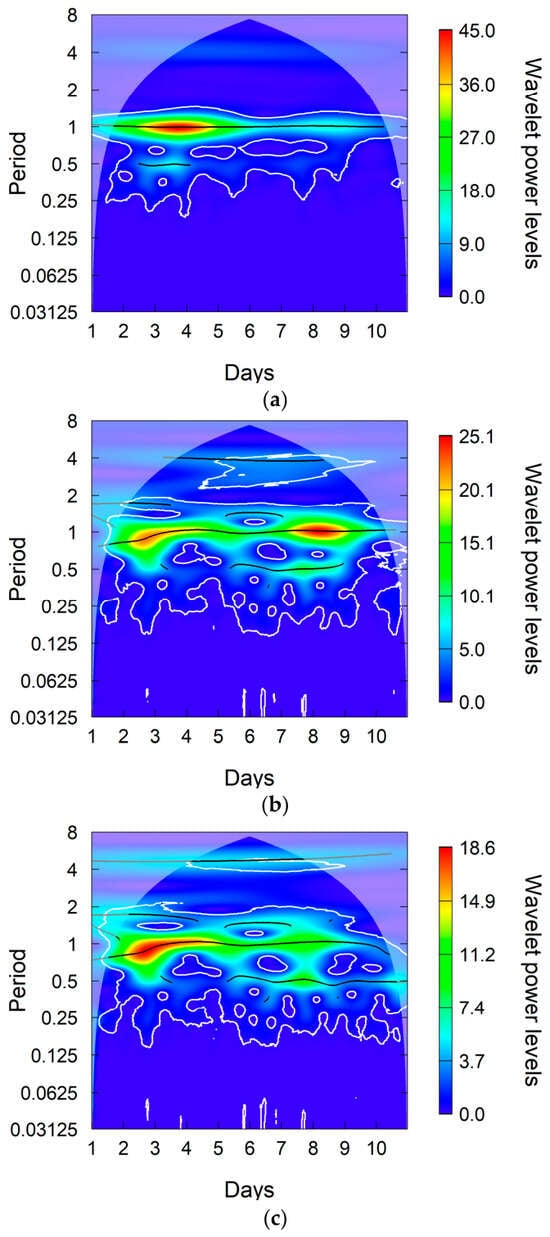
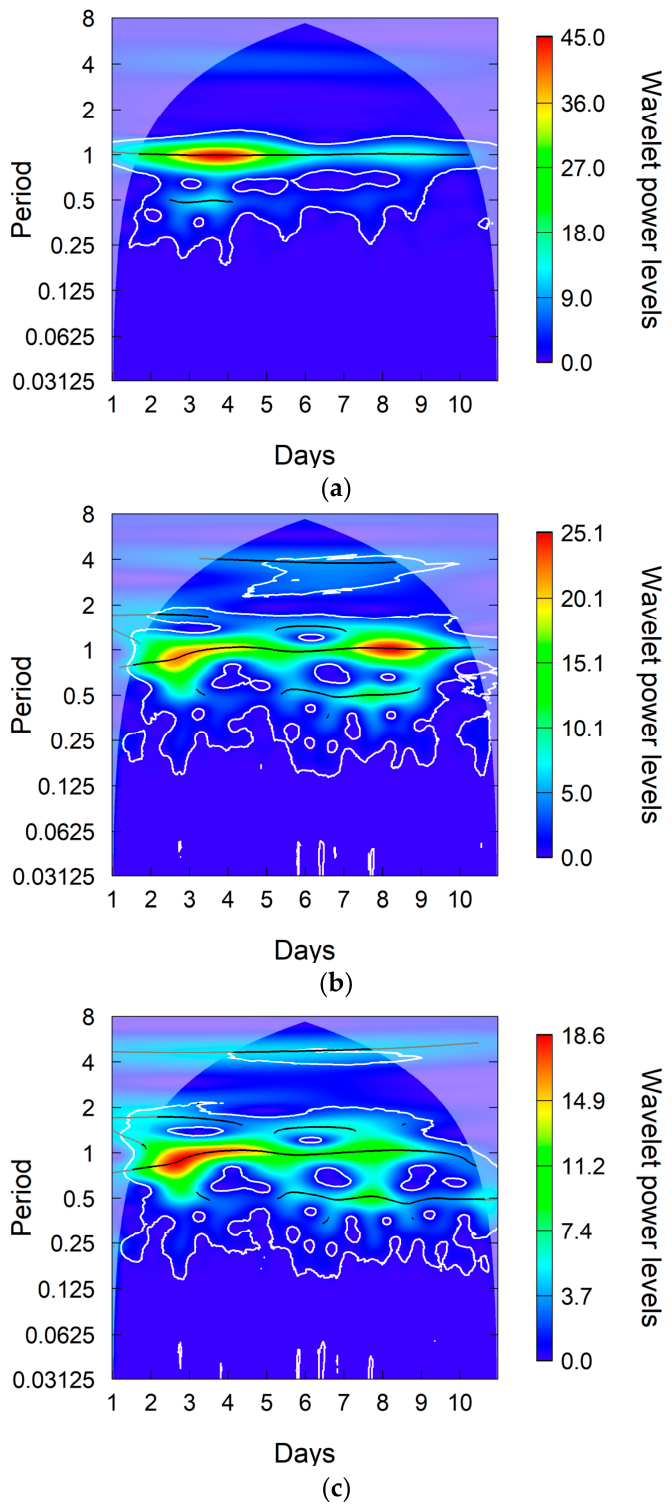
Figure 1 shows the wavelet analysis based on smoothed indoor temperature data from the three time intervals studied. As with outdoor temperature, 24 h periodicity appears clearly in all three intervals, and 12 h periodicity appears less intensely. Significant values were also obtained at various points in the 8 h periods and were more abundant in the last two intervals.
Figure 1.
Wavelet Power Spectra depicting the indoor temperature (TIND) series for each time interval: (a) 1; (b) 2; (c) 3.
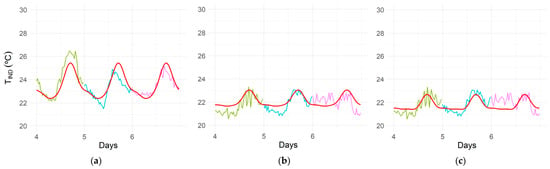
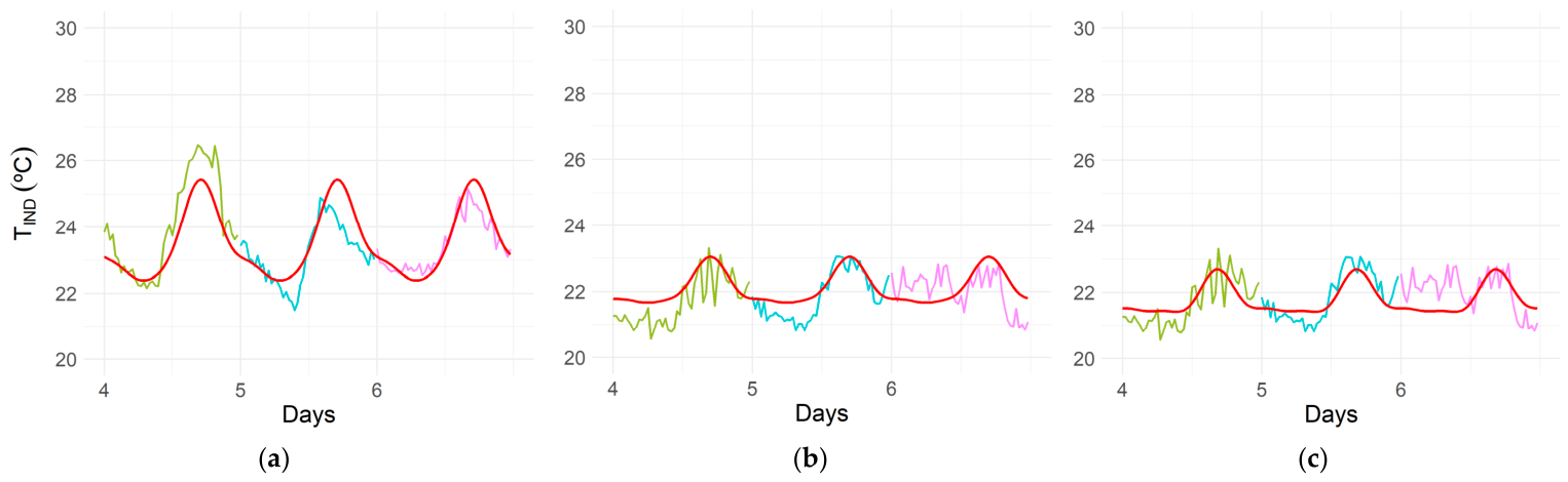
The three-harmonic cosine model fit (Table 4) shows a slight decrease in the average value (A0), reflecting lower target temperatures as animal weight increased. However, as a controlled variable inside the pig room, variation was much milder even though influenced by the outside. Accordingly, the amplitude values were smaller and decreased from the first harmonic (A1) to the second (A2) and third (A3), which was very reduced. As with outdoor temperature, the night/day thermal oscillation was represented well in the cosine model, but unlike outdoor temperature, no major differences appeared in the evolution of different days (Figure 2 and Table 5).
Table 4.
Cosine model fit to indoor temperature, TIND: A0, A1, A2, and A3 indicate the mean and amplitudes of the first, second, and third harmonic of the fit, respectively, and , , and represent the initial angles of each harmonic.
Figure 2.
Fit of the cosine model to the evolution of indoor temperature (TIND) in the pig room, measured on days 4—, 5— and 6—, and modelling days—, of each time interval studied: (a) 1; (b) 2; (c) 3.
Table 5.
Goodness-of-fit statistics for the cosine model of indoor temperature (TIND). Root Mean Square Error (RMSE), Symmetric Mean Absolute Percentage Error (sMAPE), and Determination coefficient (R2) were calculated using normalized values, whereas RMSED corresponds to the root mean square error calculated from the original (non-normalized) temperature values and is expressed in °C.
3.2. Outdoor Temperature
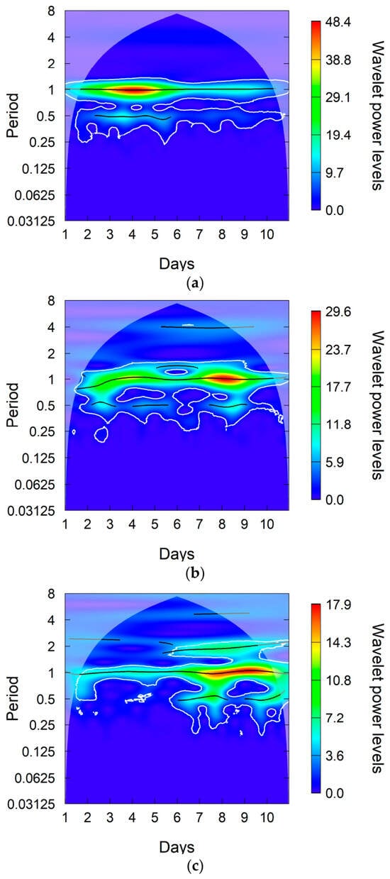
Figure 3 shows the wavelet analysis using the smoothed data corresponding to outdoor temperature in the three study intervals. The 24 h periodicity appears clearly in all three intervals, while the less intense 12 h periodicity is also detectable most of the time in each interval.
Figure 3.
Wavelet Power Spectra depicting the outdoor temperature (TOUT) series for each time interval studied: (a) 1; (b) 2; (c) 3.
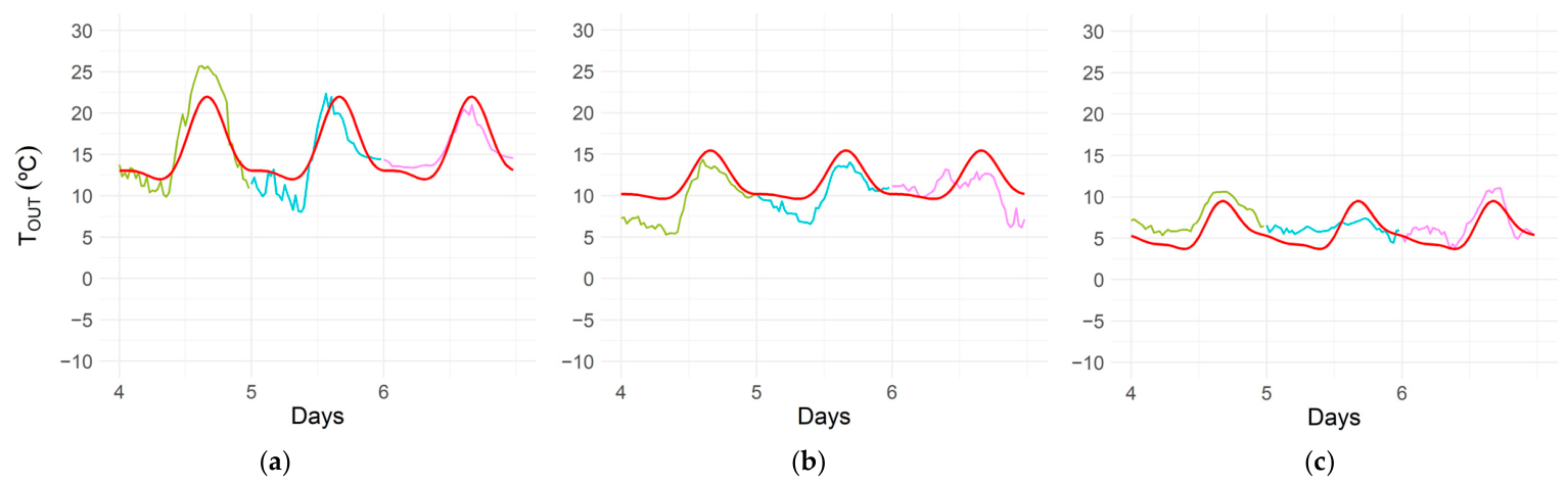
The fit to a three-harmonic cosine model (Table 6) revealed a decrease in average value (A0) over time as the production cycle advanced into winter. Amplitude also diminished, with the highest values for the first harmonic (A1), followed by the second (A2), and a clear decrease in the third (A3), which confirms the results of the wavelet analysis. In general, night/day thermal oscillation was represented well in the cosine model. The minimum temperatures that originally occurred from 8:00 a.m. to 10:00 a.m. occupied more of the day as the production cycle progressed, and maximum values were recorded at around 4:30 to 5:00 p.m. However, this oscillation did not occur on days 1, 4, 6, 8 and 10 of the second interval or days 2, 5 and 9 of the third interval. Those days either presented asymmetrical patterns due to rising or falling temperatures or were very flat, which detracts from the representativeness of the cosine model (Figure 4 and Table 7).
Table 6.
Fit of the cosine model to outdoor temperature, TOUT: A0, A1, A2 and A3 indicate the mean and amplitudes of the first, second, and third harmonic of the fit, respectively, and , , and represent the initial angles of each harmonic.
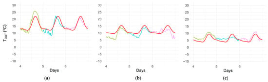
Figure 4.
Fit of the cosine model to the evolution of outdoor temperature (TOUT) on the pig farm, measured on days 4—, 5— and 6—, and modelling days—, of each time interval studied: (a) 1; (b) 2; (c) 3.
Table 7.
Goodness-of-fit statistics for the cosine model of indoor temperature (TOUT). Root Mean Square Error (RMSE), Symmetric Mean Absolute Percentage Error (sMAPE), and Determination coefficient (R2) were calculated using normalized values, whereas RMSED corresponds to the root mean square error calculated from the original (non-normalized) temperature values and is expressed in °C.
3.3. CO2 Concentration
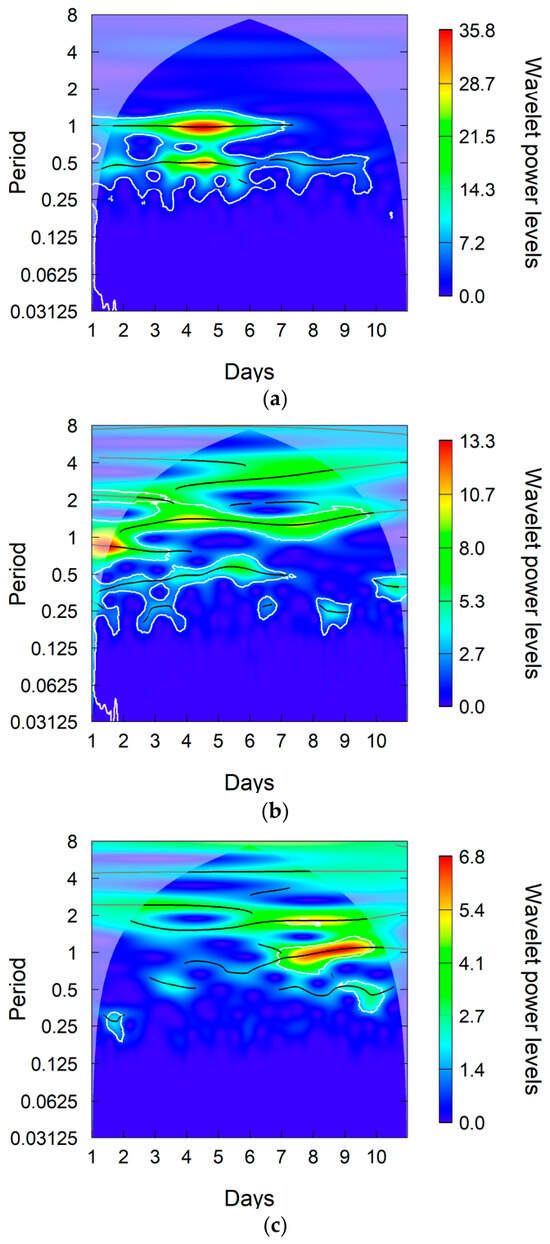
Figure 5 shows the wavelet analysis based on the smoothed data for CO2 concentration in the three time intervals studied.
Figure 5.
Wavelet Power Spectra depicting the CCO2 series for each time interval: (a) 1; (b) 2; (c) 3.
In the first interval, 24 h and 12 h periodicities were very clear, and the 8 h periodicity somewhat less so. In the second interval, the wavelet analysis showed no stable periodicity. The third interval presented intermediate behaviour with respect to the other two. CCO2 evolution did not display the three periodicities as plainly as in the first interval, but the 24 h period was clearly observed in the final half of the interval. The 12 h period was identified during days 3 and 4 and from day 7 on, while the 8 h period appeared only occasionally.
These results led to a three-harmonic sinusoidal model (Table 8), with a fit showing an increasing average value (A0) of CO2 concentration as the production cycle advanced. Amplitudes had greater weight in the first interval, with even values for the first (A1) and second (A2) harmonics, then a clear decrease in the third (A3). The loss of oscillation detected by the wavelet analysis in the second interval is reflected in low amplitude values. Though they expand again in the third interval, they remain clearly diminished compared to the first harmonic and of less relative importance than the second harmonic.
Table 8.
Fit of the cosine model to CO2 concentration, CCO2: A0, A1, A2 and A3 indicate the mean and amplitudes of the first, second, and third harmonic of the fit, respectively, and , , and represent the initial angles of each harmonic.
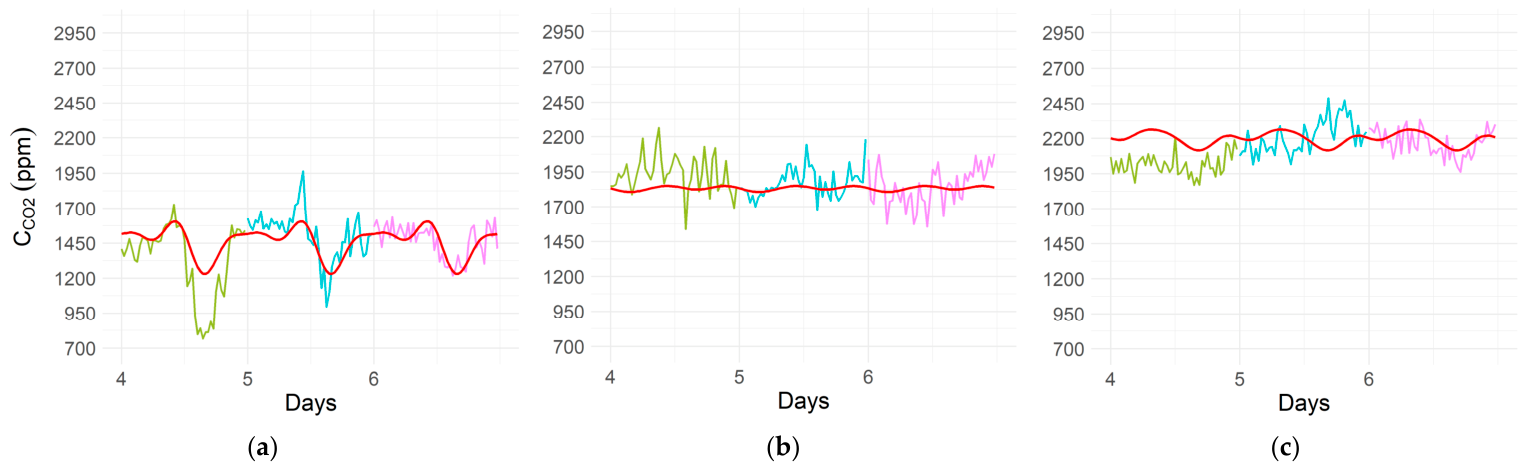
The overall fit in the first interval is good, as it adequately describes CCO2 evolution (Figure 6): high nighttime concentration and a morning peak followed by lower levels in the afternoon that increase again during the last hours of the day. The 12 h periodicity was very clearly detected, but the 8 h periodicity appeared more diffuse and intermittent. Normalized error values in this interval (Table 8) were acceptable and consistent with the wavelet analysis results. In the second interval, due to the loss of daily periodicity in CCO2 that was already observable at the end of the first interval, it was difficult to fit the evolution of the variable to the harmonic model. Therefore, the harmonic model cannot describe this erratic evolution. Although wavelet analysis showed three periodicities during the first days, this behaviour gave way to highly variable periodicities, none of which presented sufficient stability to define the wave behaviour. Although RMSE values showed a small increase and sMAPE even decreased, this behaviour is manifested as a clear decrease in the R2 value (Table 9). The model fit for the third interval revealed a similar but more subtle trend to that described for CCO2 evolution in the pig room during the first interval. The R2 value for the third interval falls between those of the prior two intervals (Table 9).
Figure 6.
Fit of the cosine model to the evolution of CCO2 measured in the pig room on days 4—, 5— and 6—, and modelling days—, of each time interval studied: (a) 1; (b) 2; (c) 3.
Table 9.
Goodness-of-fit statistics for the cosine model of CO2 concentration (CCO2). Root Mean Square Error (RMSE), Symmetric Mean Absolute Percentage Error (sMAPE), and Determination coefficient (R2) were calculated using normalized values, whereas RMSED corresponds to the root mean square error calculated from the original (non-normalized) concentration values and is expressed in ppm.
3.4. Animal Activity
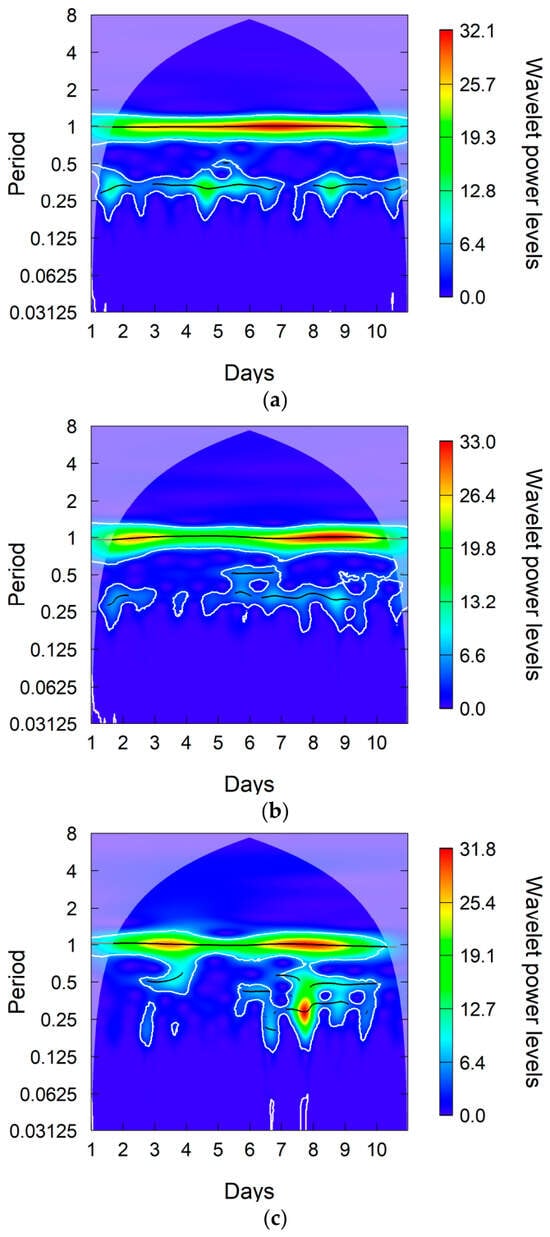
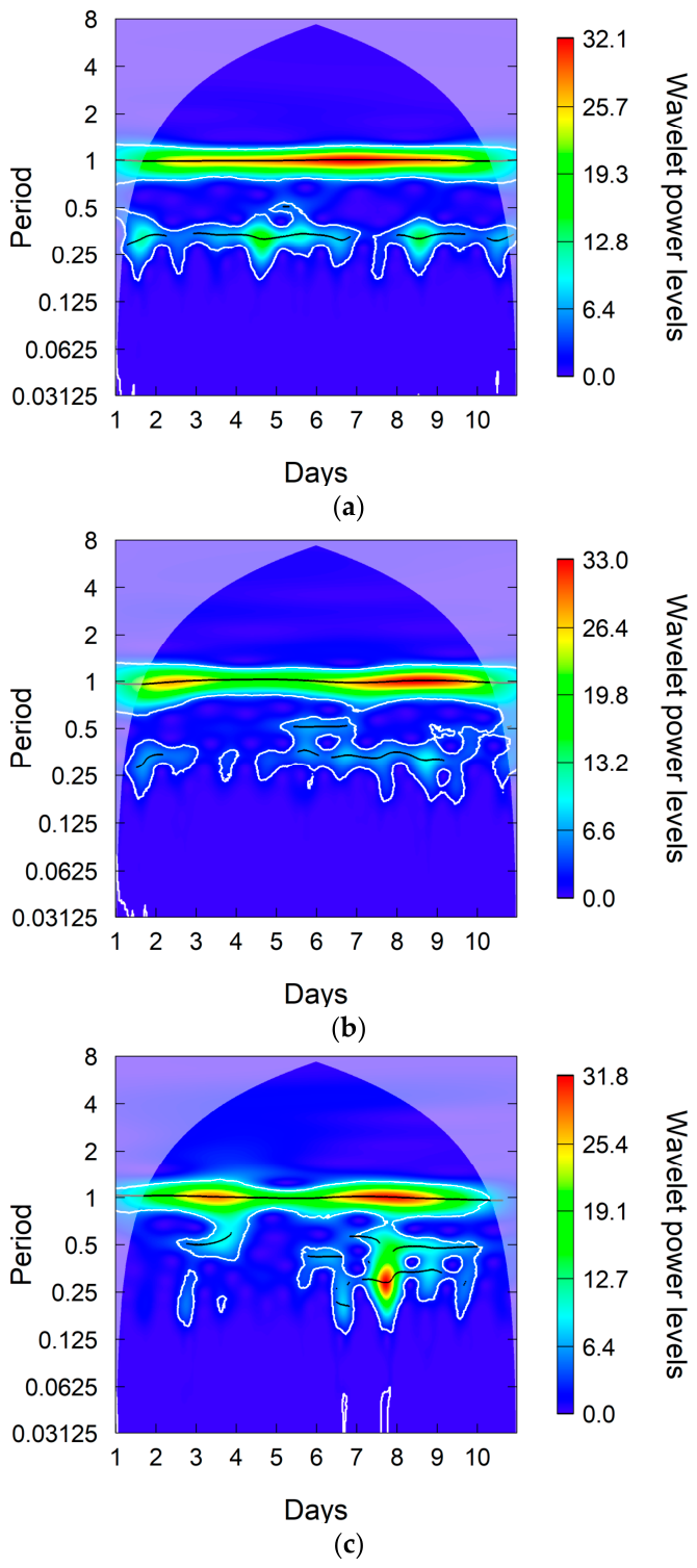
Figure 7 shows the wavelet analysis based on the smoothed data for animal activity in the three time intervals studied. In all of them, 24 h periodicity is abundantly clear. The 12 h period appears intermittently and less prominently than the 8 h period, which displays some discontinuity in most of the first two intervals and appears very clearly in the second half of the third interval.
Figure 7.
Wavelet Power Spectra depicting the animal activity (AANI) series for each of the three intervals: (a) 1; (b) 2; (c) 3.
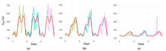
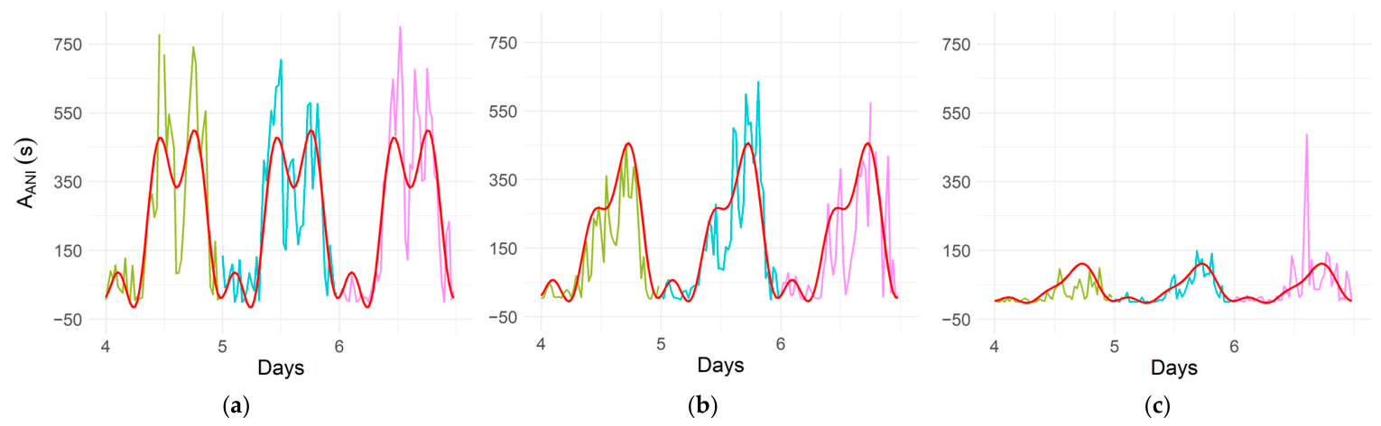
The results support the use of the cosine model of three harmonics (Table 10), which has conditioned all the other variables. Average animal activity values decreased dramatically over the production cycle, especially in the last interval, as indicated by the A0 term in the model. The highest amplitude was obtained for the first harmonic (A1, 24 h), followed by the third harmonic (A3, 8 h) in the first two intervals and the second harmonic (A2, 12 h) in the third interval. The cosine adjustment accurately represents the evolution of animal activity (Figure 8, Table 11), which, during the first interval, presented two daily peaks around noon and 7 p.m., with lower nighttime values. The second interval presented a smaller midday peak, and the absolute maximum occurred during the early evening, at around 6:30 p.m. In the third interval, activity declined drastically and was clearly concentrated in a single afternoon peak.
Table 10.
Fit of the cosine model to animal activity: Where A0, A1, A2 and A3 indicate the mean and amplitudes of the first, second, and third harmonic of the fit, respectively, and , , and are the initial angles of each harmonic.
Figure 8.
Fit of the cosine model to the evolution of mean animal activity, AANI, measured in the pig room on days 4—, 5— and 6—, and modelling days—, of each time interval studied: (a) 1; (b) 2; (c) 3.
Table 11.
Goodness-of-fit statistics for the cosine model animal activity (AANI Root Mean Square Error (RMSE), Symmetric Mean Absolute Percentage Error (sMAPE), and Determination coefficient (R2) were calculated using normalized values, whereas RMSED corresponds to the root mean square error calculated from the original (non-normalized) concentration values and is expressed in s.
3.5. Coherence Analysis
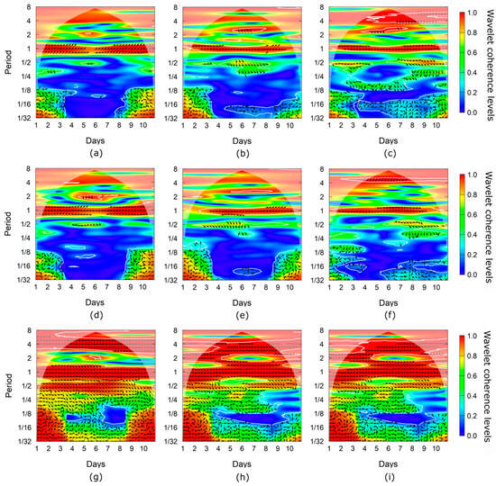
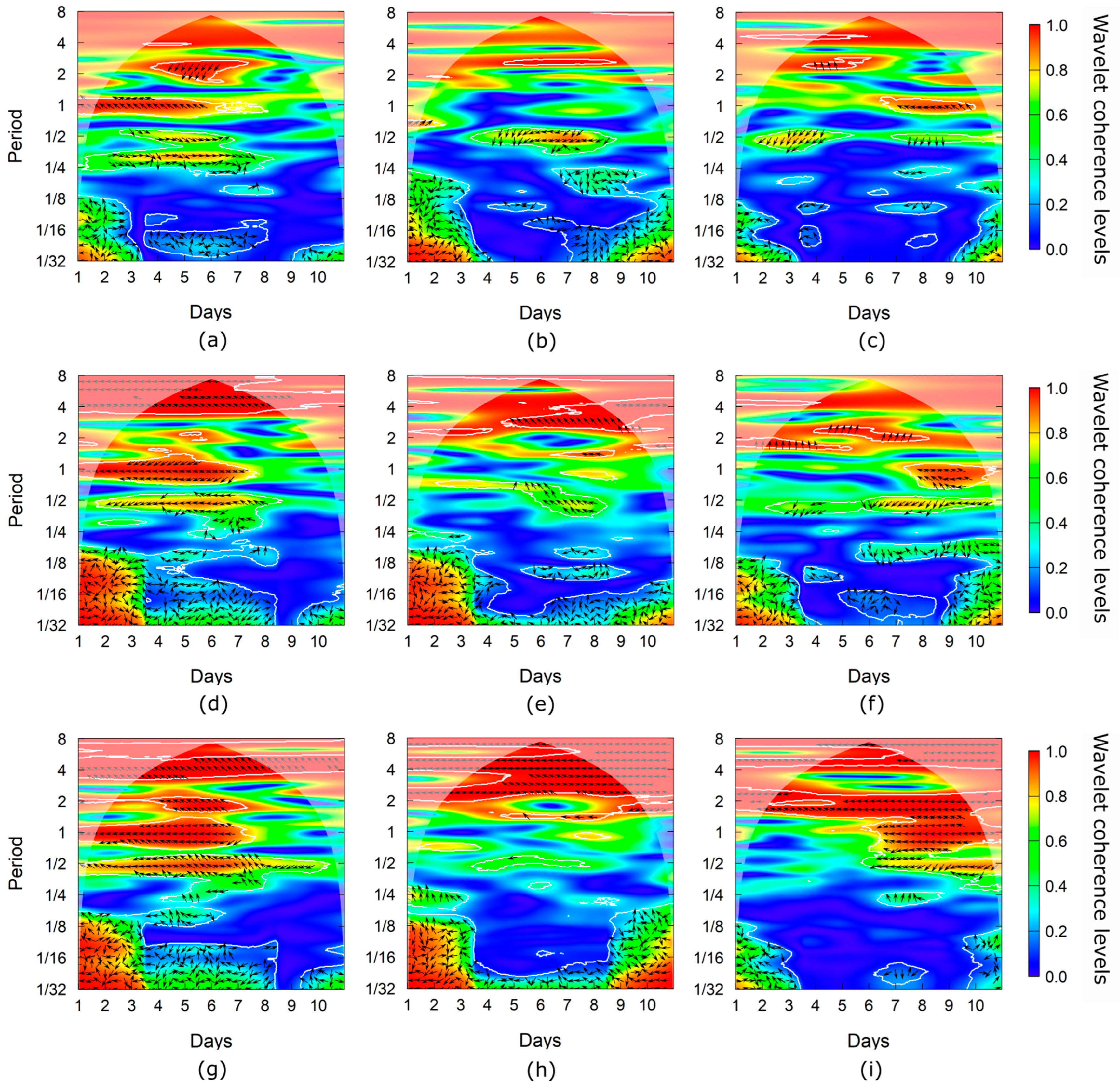
The coherence analysis results for all the variables studied are shown in Figure 9 and Figure 10. The ordinate axis (y) represents the period, with the value 1 corresponding to one day or the first harmonic in the cosine model, and the abscissa axis (x) displays the days of each time interval studied in the fattening cycle. Figure 9 and Figure 10 both show the consistency levels obtained for the different periods. When coherence is high, the relationship between the variables is also indicated with a vector representing the phase difference in the evolution of the variables: a concept similar to the initial phase angle presented by cosine models. An angle of 0 r means parallel evolution of the variables: they are in phase. An angle of π implies antiphase evolution: when one variable has high values, the other will have low values and vice versa. From this, phase differences are identified and expressed as leads or lags between variables, considering that the angle 2 π r corresponds to the time of the period analyzed.
Figure 9.
Wavelet Coherence Spectra depicting animal activity (AANI) in relation to outdoor and (TOUT) indoor temperatures (TIND) for each time interval: (a) AANI × TIND Interval 1; (b) AANI × TIND Interval 2; (c) AANI × TIND Interval 3; (d) AANI × TOUT Interval 1; (e) AANI × TOUT Interval 2; (f) AANI × TOUT Interval 3; (g) TIND × TOUT Interval 1; (h) TIND × TOUT Interval 2; (i) TIND × TOUT Interval 3. Colours represent the wavelet coherence level, with warmer colours indicating stronger coherence. White contours delimit statistically significant regions (90% confidence level). Within these regions, arrows indicate the phase relationship between the variables: arrows pointing to the right denote in-phase behaviour, arrows pointing to the left indicate antiphase behaviour, and intermediate directions represent phase leads or lags, considering the analyzed period as one complete cycle (2π).
Figure 10.
Wavelet Coherence Spectra depicting CO2 concentration (CCO2) in relation to animal activity (AANI) and outdoor (TOUT) and indoor (TIND) temperatures for each time interval: (a) CCO2 × AANI Interval 1; (b) CCO2 × AANI Interval 2; (c) CCO2 × AANI Interval 3; (d) CCO2 × TIND Interval 1; (e) CCO2 × TIND Interval 2; (f) CCO2 × TIND Interval 3; (g) CCO2 × TOUT Interval 1; (h) CCO2 × TOUT Interval 2; (i) CCO2 × TOUT Interval 3. Colours represent the wavelet coherence level, with warmer colours indicating stronger coherence. White contours delimit statistically significant regions (90% confidence level). Within these regions, arrows indicate the phase relationship between the variables: arrows pointing to the right denote in-phase behaviour, arrows pointing to the left indicate antiphase behaviour, and intermediate directions represent phase leads or lags, considering the analyzed period as one complete cycle (2π).
Figure 9 shows the high coherence between animal activity and indoor and outdoor temperatures in the fundamental period (1 day) and, to a lesser extent and less permanently, in the 1/2 (12 h) period. Significant levels of coherence were also observed, most intensely between animal activity and indoor temperature, when ventilation was limited by low outdoor temperatures (days 9–10 of the first interval, days 5–8 of the second interval, and days 7–10 of the third interval) or by high thermal requirements at the beginning of the cycle. This finding supports the contribution of animal activity to higher indoor temperatures.
In the fundamental period, a relationship between animal activity and temperatures was established around the antiphase. In the 1/2 period, the relationship evolved from antiphase in the first interval to 90° leads (equivalent to 3 h) in the second interval and to leads close to 30° (equivalent to 1 h) in the third interval, with animal activity lagging behind temperature in the latter two cases. Some significant coherence levels appeared in the 1/3 period at a phase difference of around 90°, indicating a 2 h lead of temperature with respect to animal activity.
High levels of coherence were found between animal activity and CO2 concentration inside the pig room in all the time intervals analyzed (Figure 10). Although somewhat less prominent in the second interval, the fundamental period (1 day) in the first and third intervals presents more permanence and coherence in a relation approaching antiphase to high coherences. While the ½ period (12 h) appears in all three intervals, the variables shift from being in phase with parallel variation in the first interval, to an antiphase relationship during much of the second interval, to presenting angles (0.58–0.75 π r) associated with a lag of 7–9 h in animal activity in the third interval. Additionally, high and persistent coherence was clearly seen in the 1/3 period (8 h) during the first interval, with both variables in phase. This corresponds to the results obtained for the cosine model, in which CO2 concentration and animal activity present a significant amplitude value for the third harmonic.
High levels of coherence with outdoor and indoor temperatures accompanied the evolution of CO2 concentration. In the first interval, the variables presented high coherence and antiphase in the fundamental period, with values decreasing at the end of the interval. In the second interval, average levels were detected for both temperatures at specific points at the end. In the third interval, coherence increased after the first 3 days in antiphase with outside and inside temperature. The 1/2 period had lower coherence values but was present in all three intervals and for outdoor and indoor temperatures. The relation of CO2 concentration to outdoor temperature was more intense and near antiphase in the first time interval and the second half of the third interval. Coherence levels with indoor temperature also remained high in the second interval.
4. Discussion
As the animals grew, CO2 concentration in the pig room steadily increased. From an average value of 1459 ppm in the first interval, CO2 levels rose by 26% and 52% in the consecutive intervals. This coincides with what Deb et al. [31] described in association with the increasing body mass of the animals [5]. Meanwhile, compared to the first interval, animal activity decreased to 75% and 15% in the second and third intervals. This highlights the strong influence of animal age and weight, which may be conditioned by higher animal density [20]. Decreased animal activity could also be related to higher CO2 concentration as the cycle progresses [34]. In naturally ventilated facilities, outdoor temperature was strongly associated with indoor climate dynamics, resulting in patterns characterized primarily by 24 h periods and to a lesser extent by 12 h periods, as seen in the wavelet analysis results. Indoor temperature also presented significant influence in the 8 h period, most notably during the latter intervals of the production cycle. These findings suggest that animal activity became more closely associated with indoor temperature variability, particularly as animal weight increased and ventilation became more limited due to low outdoor temperatures.
The behaviour of CCO2 did not settle into a consistent oscillatory pattern in all intervals. It was more stable in the 12 h period and presented high, dominant intensities during the 24 h period in the first part of the first interval and the second part of the third interval. This dynamic made it possible to obtain cosine models with a very good fit for the first interval and a good fit for the third interval, with well-defined variations featuring higher concentrations during the night, a morning peak, a decrease during the afternoon, then another increase. However, a good fit of the cosine model could not be obtained for the second interval due to low CCO2 variation. Unlike the mechanically ventilated weaned piglet facility studied by Fernández et al. [7], where CO2 exhibited a more stable temporal pattern, the naturally ventilated fattening pig house showed less persistent oscillatory behaviour. This difference is likely attributable to the greater influence of outdoor climatic conditions and natural ventilation on the indoor environment.
For animal activity, the 24 h period predominated, followed by the 8 h period and the more sporadic 12 h period. This gave rise to initial daily patterns characterized by two peaks of similar magnitude in daytime activity and a rest period during the hottest hours [2,7,33]. As the animals grew, the morning activity peak decreased steadily to near extinction in the third interval, when animal activity was mainly concentrated into a single daily peak during the afternoon. This may also have been influenced by the reduced daylight hours that accompany the onset of winter.
By applying cosine models of three harmonics selected from the wavelet analysis results, important differences among the variables came to light. For temperature, the RMSE over normalized values proved very adequate, with maximum values of 0.10. Similarly, the coefficient of determination (R2) ranged between 0.65 and 0.84 for outdoor temperature and had slightly lower values of 0.52 to 0.78 for indoor temperature. In both cases, predictive quality decreased as the production cycle progressed. These results were improved by machine-learning-based models, specifically random forest regression [39,40,42] or deep-learning techniques [43], which rendered R2 values greater than 0.9. In contrast, ARIMA statistical models ranged from 0.52 to 0.81, providing R2 values very similar to those of Ortega et al. [50].
Despite their lower predictive accuracy compared with advanced machine-learning and deep-learning approaches, the proposed harmonic models offer several practical advantages for implementation in current naturally ventilated pig houses. Environmental control systems are commonly based on programmable logic controllers (PLCs) that regulate ventilation using indoor temperature as the primary control variable. These controllers execute cyclic programmes with limited computational capacity, relying on real-time clocks and basic mathematical functions. Since the proposed models require only time as the input variable, they can be readily implemented within existing PLC-based control systems, without additional sensors, computing hardware or major modifications to the current control architecture. Furthermore, different harmonic models could be associated with the temperature setpoints routinely used throughout the production cycle, allowing the estimation of environmental and behavioural variables under different production stages.
Loss of the oscillatory character of CO2 concentration, as revealed by the wavelet analysis, explains the limited fit of the cosine model. Although acceptable RMSE values (0.14) were obtained, the maximum coefficient of determination (R2) remained low (0.39) in the first interval. These results are lower than others reported for piglets using machine-learning techniques, such as neural networks [44] or random forest regression [42], or deep-learning models [43]. The results are also lower than those obtained for fattening pigs using statistical models, namely multiple linear regression [5] and exponential regression [48]. This contrasts with the improved results from applying the cosine model to animal activity, with RMSE values ranging from 0.06 to 0.16 and R2 values between 0.43 and 0.71. These values are acceptable, considering the simplicity of the model and the inherent complexity of modelling animal behaviour. This different predictive performance reflects the temporal behaviour identified by the wavelet analysis. Variables exhibiting stable periodicities, such as indoor and outdoor temperature and, to a lesser extent, animal activity, were more accurately represented by harmonic models, whereas the irregular oscillatory behaviour of CO2 concentration limited the suitability of this approach.
Since the pig room was naturally ventilated, indoor and outdoor temperatures exhibited high wavelet coherence, especially in the 24 h and 12 h periods. In both cases, the outdoor temperature exhibited a phase lead of approximately 1 h relative to the indoor temperature. This temporal relationship is consistent with the thermal inertia of the pig room, although wavelet coherence does not by itself establish a causal relationship. The exception to this pattern occurred during the third interval: when outdoor temperatures fell below 0 °C, the phase difference reversed, and indoor temperature led outdoor temperature due to the drastic reduction in ventilation rates. A similar decrease in coherence was also detected in the 12 h period during the first four days of the third interval.
Carbon dioxide concentration presented a close relationship with outside and inside temperature, especially in the first and third intervals. The 24 h period showed the highest levels of coherence, reflecting the high daily outdoor thermal range, while the 12 h period presented a more persistent relation to indoor temperature. In both periods, CCO2 evolved in antiphase with temperatures. Higher CCO2 coincided with lower outdoor [7] and indoor temperatures, a temporal relationship consistent with reduced ventilation and the consequent accumulation of gas inside the building [21,44]. This was especially apparent in the increased coherence between CCO2 and indoor temperature during the 24 and 12 h periods.
Animal activity also displayed high coherence with temperatures in the 24 and 12 h periods, mainly, and presented a slight lead of 1 to 2 h with respect to temperatures for the 24 h period. Meanwhile, the relationship between animal activity and CO2 concentration showed stable phase differences of nearly 10 h in the 24 h period of the first interval but were less defined in the third. In the 12 h period, animal activity consistently lagged 7 to 9 h behind CCO2 throughout the cycle. A strong relationship only appeared in the first interval for the 8 h period, reflecting the high temporal instability of both variables. Although wavelet coherence analysis provides valuable information on localized time-frequency associations and phase relationships, these results should be interpreted as evidence of temporal synchronization rather than direct causal interactions between variables.
This study has several limitations that should be considered. Although continuous measurements throughout the entire production cycle would have been preferable, the selected intervals covered the beginning, middle and end of the fattening cycle and included sufficient temporal and environmental variability to achieve the objectives of the study. Nevertheless, unrecorded periods may have contained transient behaviours that were not captured in the present analysis. Furthermore, purged K-fold cross-validation provides a robust assessment of internal predictive performance and minimizes information leakage. However, the proposed models were developed and validated using data from a single production cycle in one commercial livestock facility operating under specific environmental and management conditions. Therefore, further validation using independent production cycles, different farms and climatic conditions is required before extending the applicability of the proposed models to other naturally ventilated pig-housing systems.
5. Conclusions
From this study of the environmental variables of indoor and outdoor temperatures along with CO2 concentration and the animal variable of activity in a naturally ventilated pig-fattening facility evaluated in this study, the following conclusions can be established:
The wavelet analysis made it possible to characterize the temporal evolution of the variables and identify dominant periods of 24 and 12 h for indoor and outdoor temperatures. Animal activity showed an additional relevant contribution from the 8 h period. In contrast, CO2 concentration did not present a stable daily oscillatory pattern throughout the fattening cycle.
The application of three harmonic cosine models (24 h, 12 h and 8 h) provided a satisfactory fit for outdoor temperatures (RMSE = 0.09–0.10, R2 = 0.65–0.84), indoor temperatures (RMSE = 0.08–0.10, R2 = 0.52–0.78) and animal activity (RMSE = 0.06–0.16, R2 = 0.43–0.61). This approach was not suitable for predicting CO2 concentration, as this variable did not present stable oscillatory behaviour over the production cycle. Nonetheless, the animal activity model remains especially relevant given the difficulty of integrating animal behaviour variables into similar livestock housing control systems.
The wavelet coherence analysis proved useful for characterizing time-frequency relationships and phase differences among complex temporal variables and made it possible to identify 1 h lags of indoor interior temperature with respect to outdoor temperature over the 24 h and 12 h periods. These phase relationships suggest that outdoor temperature may provide useful information for anticipating indoor temperature changes and could therefore contribute to predictive temperature-control strategies in naturally ventilated pig-fattening systems considered in this study. Though not persistent, CO2 concentration presented antiphase relationships with temperatures during some periods of the fattening cycle. Additionally, animal activity showed a lead of 1 to 2 h with respect to temperatures for the 24 h period.
While cosine models have lower predictive performance than advanced machine-learning or deep-learning techniques, their low computational requirements and compatibility with conventional PLC-based environmental controllers make them an attractive alternative for improving environmental control in naturally ventilated livestock buildings without additional sensing or computing infrastructure. Temporal relationships derived from the coherence analysis may provide valuable information for supporting the design and optimization of control strategies in livestock facilities with air conditioning systems characterized by heterogeneous thermal inertia and response dynamics based on the variable considered and the equipment used. The results suggest that these tools have the potential to improve the understanding of microclimate dynamics and to support the development of simplified control strategies for naturally ventilated pig housing.
Author Contributions
Conceptualization, M.D.F. and M.R.R.; methodology, S.H.-F. and R.B.; software, S.H.-F. and R.B.; validation, S.H.-F. and R.B.; formal analysis, S.H.-F. and R.B.; investigation, M.D.F. and M.R.R.; resources, M.D.F. and M.R.R.; data curation, M.D.F. and M.R.R.; writing—original draft preparation, M.D.F. and M.R.R.; writing—review and editing, S.H.-F. and R.B.; visualization, S.H.-F. All authors have read and agreed to the published version of the manuscript.
Funding
This research was funded by the Xunta de Galicia, grant number ED431B 2021/08 and grant number ED431B2024/13.
Institutional Review Board Statement
Directive 2010/63/EU on the protection of animals used for scientific purposes was not applicable, since the animals were raised solely for commercial production and no experimental manipulation beyond environmental monitoring was performed. Consequently, ethical approval was not required for the present study.
Data Availability Statement
Data will be made available on request.
Conflicts of Interest
The authors declare no conflicts of interest.
Abbreviations
The following abbreviations are used in this manuscript:
| A0 | Independent term in the cosine model |
| A1 | Amplitude of the first harmonic with a period of 24 h |
| A2 | Amplitude of the second harmonic with a period of 12 h |
| A3 | Amplitude of the third harmonic with a period of 8 h |
| AANI | Animal activity, s |
| CCO2 | CO2 concentration, ppm |
| CWT | Continuous Wavelet Transforms |
| p | autoregressive order |
| q | moving average order |
| R2 | Coefficient of determination |
| RMSE | Root Mean Square Error |
| sMAPE | Symmetric Mean Absolute Percentage Error |
| t | Time, h |
| TIND | Indoor temperature, °C |
| TOUT | Outdoor temperature, °C |
| φ1 | Initial phase angle for the first harmonic |
| φ2 | Initial phase angle for the second harmonic |
| φ3 | Initial phase angle for the third harmonic |
References
- Gibson, T.J.; Jackson, E.L. The economics of animal welfare. Rev. Sci. Tech. Int. Off. Epizoot. 2017, 36, 125–135. [Google Scholar] [CrossRef] [Scilit] [PubMed]
- Huynh, T.T.T.; Aarnink, A.J.A.; Gerrits, W.J.J.; Heetkamp, M.J.H.; Canh, T.T.; Spoolder, H.A.M.; Kemp, B.; Verstegen, M.W.A. Thermal behaviour of growing pigs in response to high temperature and humidity. Appl. Anim. Behav. Sci. 2005, 91, 1–16. [Google Scholar] [CrossRef] [Scilit]
- Chantziaras, I.; De Meyer, D.; Vrielinck, L.; Van Limbergen, T.; Pineiro, C.; Dewulf, J.; Kyriazakis, I.; Maes, D. Environment-, health-, performance-and welfare-related parameters in pig barns with natural and mechanical ventilation. Prev. Vet. Med. 2020, 183, 105150. [Google Scholar] [CrossRef] [Scilit] [PubMed]
- Ma, H.; Wang, S.; Gu, J.; Xie, Q.; Wang, W.; Dong, S.; Sun, C.; Li, J.; Ma c Dong, J.; Liu, H. IoT-based smart environmental control and air emission management in animal farming: A systematic review. Inf. Process. Agric. 2026; in press. [CrossRef] [Scilit]
- Sun, X.; Wang, S.; Xie, Q.; Sun, C.; Yu, H.; Wang, W. Variations of multiple environmental factors and multi-objective optimisation control in a pig house. Biosyst. Eng. 2025, 259, 104300. [Google Scholar] [CrossRef] [Scilit]
- Guo, Z.; Yin, Z.; Lyu, Y.; Wang, Y.; Chen, S.; Li, Y.; Zhang, W.; Gao, P. Research on indoor environment prediction of pig house based on OTDBO–TCN–GRU algorithm. Animals 2024, 14, 863. [Google Scholar] [CrossRef] [Scilit] [PubMed]
- Fernandez, M.D.; Rodriguez, M.R.; Fdez-Vidal, X.R.; Besteiro, R. Wavelet analysis and sinusoidal modelling of environmental variables in a weaned piglet farm. Build. Environ. 2025, 279, 113049. [Google Scholar] [CrossRef] [Scilit]
- Michiels, A.; Piepers, S.; Ulens, T.; Van Ransbeeck, N.; Del Pozo Sacristan, R.; Sierens, A.; Haesebrouck, F.; Demeyer, P.; Maes, D. Impact of particulate matter and ammonia on average daily weight gain, mortality and lung lesions in pigs. Prev. Vet. Med. 2015, 121, 99–107. [Google Scholar] [CrossRef] [Scilit] [PubMed]
- Zang, J.; Ye, S.; Xu, Z.; Wang, J.; Liu, W.; Bai, Y.; Yong, C.; Zou, X.; Zhang, W. Prediction model of carbon dioxide concentration in pig house based on deep learning. Atmosphere 2022, 13, 1130. [Google Scholar] [CrossRef] [Scilit]
- Li, X.; Shen, J.; Yang, X.; Nie, P.; Li, Y.; Li, Z.; Tan, Y.; Li, Z. Construction of time series prediction and dynamic evaluation model for environmental factors in pregnant sow houses in winter. Smart Agric. Technol. 2025, 12, 101125. [Google Scholar] [CrossRef] [Scilit]
- Rojo-Gimeno, C.; Postma, M.; Dewulf, J.; Hogeveen, H.; Lauwers, L.; Wauters, E. Farm-economic analysis of reducing antimicrobial use whilst adopting improved management strategies on farrow-to-finish pig farms. Prev. Vet. Med. 2016, 129, 74–87. [Google Scholar] [CrossRef] [Scilit] [PubMed]
- Raasch, S.; Collineau, L.; Postma, M.; Backhans, A.; Sjölund, M.; Belloc, C.; Emanuelson, U.; Beilage, E.G.; Stärk, K.; Dewulf, J.; et al. Effectiveness of alternative measures to reduce antimicrobial usage in pig production in four European countries. Porc. Health Manag. 2020, 6, 6. [Google Scholar] [CrossRef] [Scilit] [PubMed]
- Collin, A.; van Milgen, J.; Dubois, S.; Noblet, J. Effect of high temperature on feeding behaviour and heat production in group-housed young pigs. Br. J. Nutr. 2001, 86, 63–70. [Google Scholar] [CrossRef] [Scilit] [PubMed]
- Kouba, M.; Hermier, D.; Le Dividich, J. Influence of a high ambient temperature on lipid metabolism in the growing pig. J. Anim. Sci. 2001, 79, 81–87. [Google Scholar] [CrossRef] [Scilit] [PubMed]
- Boddicker, R.L.; Seibert, J.T.; Johnson, J.S.; Pearce, S.C.; Selsby, J.T.; Gabler, N.K.; Lucy, M.C.; Safranski, T.J.; Rhoads, R.P.; Baumgard, L.H.; et al. Gestational heat stress alters postnatal offspring body composition indices and metabolic parameters in pigs. PLoS ONE 2014, 9, e110859. [Google Scholar] [CrossRef] [Scilit] [PubMed]
- Cruzen, S.M.; Boddicker, R.L.; Graves, K.L.; Johnson, T.P.; Arkfeld, E.K.; Baumgard, L.H.; Ross, J.W.; Safranski, T.J.; Lucy, M.C.; Lonergan, S.M. Carcass composition of market weight pigs subjected to heat stress in utero and during finishing. J. Anim. Sci. 2015, 93, 2587–2596. [Google Scholar] [CrossRef] [Scilit] [PubMed]
- Chen, C.; Liu, X.; Liu, C.; Yu, C. Prediction and evaluation of environmental quality for nursing sow buildings via multisource sensor information fusion. Sci. Rep. 2025, 15, 14091. [Google Scholar] [CrossRef] [Scilit] [PubMed]
- Wu, X.; Li, Z.-Y.; Jia, A.-F.; Su, H.-G.; Hu, C.-H.; Zhang, M.-H.; Feng, J.-H. Effects of high ambient temperature on lipid metabolism in finishing pigs. J. Integr. Agric. 2016, 15, 391–396. [Google Scholar] [CrossRef] [Scilit]
- Liu, F.; Zhao, W.; Le, H.H.; Cottrell, J.J.; Green, M.P.; Leury, B.J.; Dunshea, F.R.; Bell, A.W. What have we learned about the effects of heat stress on the pig industry? Animal 2022, 16, 100349. [Google Scholar] [CrossRef] [Scilit] [PubMed]
- Zong, C.; Zhang, G.; Feng, Y.; Ni, J.Q. Carbon dioxide production from a fattening pig building with partial pit ventilation system. Biosyst. Eng. 2014, 126, 56–68. [Google Scholar] [CrossRef] [Scilit]
- Buoio, E.; Cialini, C.; Costa, A. Air quality assessment in pig farming: The Italian classyfarm. Animals 2023, 13, 2297. [Google Scholar] [CrossRef] [Scilit] [PubMed]
- Pedersen, S.; Blanes-Vidal, V.; Jørgensen, H.; Chwalibog, A.; Haeussermann, A.; Heetkamp, M.J.W.; Aarnink, A.J.A. Carbon dioxide production in animal houses: A literature review. Agric. Eng. Int. CIGR J. 2008, 10, 1–19. [Google Scholar]
- Philippe, F.X.; Nicks, B. Review on greenhouse gas emissions from pig houses: Production of carbon dioxide, methane and nitrous oxide by animals and manure. Agric. Ecosyst. Environ. 2015, 199, 10–25. [Google Scholar] [CrossRef] [Scilit]
- Blanes, V.; Pedersen, S. Ventilation flow in pig houses measured and calculated by carbon dioxide, moisture and heat balance equations. Biosyst. Eng. 2005, 92, 483–493. [Google Scholar] [CrossRef] [Scilit]
- Chmielowiec-Korzeniowska, A.; Tymczyna, L.; Wlazło, Ł.; Trawińska, B.; Ossowski, M. Emissions of gaseous pollutants from pig farms and methods for their reduction—A review. Ann. Anim. Sci. 2022, 22, 89–107. [Google Scholar] [CrossRef] [Scilit]
- Zhang, L.; Zhang, M.; Yu, Q.; Su, S.; Wang, Y.; Fang, Y.; Dong, W. Optimizing winter air quality in pig-fattening houses: A plasma deodorization approach. Sensors 2024, 24, 324. [Google Scholar] [CrossRef] [Scilit] [PubMed]
- Besteiro, R.; Rodríguez, M.R.; Fernández, M.D.; Ortega, J.A.; Velo, R. Agreement between passive infrared detector measurements and human observations of animal activity. Livest. Sci. 2018, 214, 219–224. [Google Scholar] [CrossRef] [Scilit]
- Drexl, V.; Dittrich, I.; Wilder, T.; Diers, S.; Janssen, H.; Krieter, J. Prediction of tail biting in pigs using partial least squares regression and artificial neural networks. Comput. Electron. Agric. 2024, 216, 108477. [Google Scholar] [CrossRef] [Scilit]
- Ngwabie, N.M.; Jeppsson, K.H.; Gustafsson, G.; Nimmermark, S. Effects of animal activity and air temperature on methane and ammonia emissions from a naturally ventilated building for dairy cows. Atmos. Environ. 2011, 45, 6760–6768. [Google Scholar] [CrossRef] [Scilit]
- Besteiro, R.; Arango, T.; Ortega, J.A.; Rodríguez, M.R.; Fernández, M.D.; Velo, R. Prediction of carbon dioxide concentration in weaned piglet buildings by wavelet neural network models. Comput. Electron. Agric. 2018, 143, 201–207. [Google Scholar] [CrossRef] [Scilit]
- Deb, N.C.; Basak, J.K.; Paudel, B.; Kim, N.E.; Moon, B.E.; Kim, H.T. Emission of CO2 in a livestock barn based on diurnal activities and various growing stages of pigs. Air Qual. Atmos. Health 2023, 16, 1443–1454. [Google Scholar] [CrossRef] [Scilit]
- Vitali, M.; Santolini, E.; Bovo, M.; Tassinari, P.; Torreggiani, D.; Trevisi, P. Behavior and welfare of undocked heavy pigs raised in buildings with different ventilation systems. Animals 2021, 11, 2338. [Google Scholar] [CrossRef] [Scilit] [PubMed]
- Olczak, K.; Nowicki, J.; Klocek, C. Pig behaviour in relation to weather conditions—A review. Ann. Anim. Sci. 2015, 15, 601–610. [Google Scholar] [CrossRef] [Scilit]
- Bhujel, A.; Arulmozhi, E.; Moon, B.E.; Kim, H.T. Deep-learning-based automatic monitoring of pigs’ physico-temporal activities at different greenhouse gas concentrations. Animals 2021, 11, 3089. [Google Scholar] [CrossRef] [Scilit] [PubMed]
- Khaowdang, S.; Suriyachai, N.; Imman, S.; Suwannahong, K.; Wongcharee, S.; Kreetachat, T. Application of Internet of Things Technology for Ventilation and Environmental Control in Conventional Open-Air Pig Housing Systems in Thailand. AgriEngineering 2025, 7, 165. [Google Scholar] [CrossRef] [Scilit]
- Pedersen, S.; Jørgensen, H.; Theil, P.K. Influence of Diurnal Variation in Animal Activity and Digestion on Animal Heat Production. Special Issue: 18th World Congress of CIGR. 2015. Available online: https://cigrjournal.org/index.php/Ejounral/article/view/3097/2043 (accessed on 1 May 2026).
- Lagua, E.; Mun, H.S.; Ampode, K.M.B.; Park, H.R.; Kim, Y.H.; Yang, C.J. Monitoring using artificial intelligence reveals critical links between housing conditions and respiratory health in pigs. J. Anim. Behav. Biometeorol. 2024, 12, 2024008. [Google Scholar] [CrossRef] [Scilit]
- Kang, H.J.; Bae, S.; Lee, H. Correlation of animal-based parameters with environment-based parameters in an on-farm welfare assessment of growing pigs. J. Anim. Sci. Technol. 2022, 64, 539–563. [Google Scholar] [CrossRef] [Scilit] [PubMed]
- Arulmozhi, E.; Basak, J.K.; Sihalath, T.; Park, J.; Kim, H.T.; Moon, B.E. Machine learning-based microclimate model for indoor air temperature and relative humidity prediction in a swine building. Animals 2021, 11, 222. [Google Scholar] [CrossRef] [Scilit] [PubMed]
- Gautam, K.R.; Zhang, G.; Landwehr, N.; Adolphs, J. Machine learning for improvement of thermal conditions inside a hybrid ventilated animal building. Comput. Electron. Agric. 2021, 187, 106259. [Google Scholar] [CrossRef] [Scilit]
- Peng, S.; Zhu, J.; Liu, Z.; Hu, B.; Wang, M.; Pu, S. Prediction of ammonia concentration in a pig house based on machine learning models and environmental parameters. Animals 2022, 13, 165. [Google Scholar] [CrossRef] [Scilit] [PubMed]
- Yeo, U.H.; Jo, S.K.; Kim, S.H.; Park, D.H.; Jeong, D.Y.; Park, S.J.; Shin, H.; Kim, R.W. Applicability of machine-learned regression models to estimate internal air temperature and CO2 concentration of a pig house. Agronomy 2023, 13, 328. [Google Scholar] [CrossRef] [Scilit]
- Wu, Z.; Xu, K.; Chen, Y.; Liu, Y.; Song, W. A new prediction model based on deep learning for pig house environment. Sci. Rep. 2024, 14, 31141. [Google Scholar] [CrossRef] [Scilit] [PubMed]
- Rodriguez, M.R.; Besteiro, R.; Ortega, J.A.; Fernandez, M.D.; Arango, T. Evolution and neural network prediction of CO2 emissions in weaned piglet farms. Sensors 2022, 22, 2910. [Google Scholar] [CrossRef] [Scilit] [PubMed]
- Park, J.; Jo, G.; Jung, M.; Oh, Y. Comparative Analysis of Neural Network Models for Predicting Ammonia Concentrations in a Mechanically Ventilated Sow Gestation Facility in Korea. Atmosphere 2023, 14, 1248. [Google Scholar] [CrossRef] [Scilit]
- Santoro, L.M.; D’Urso, P.R.; Arcidiacono, C.; Coco, S. Data-Driven Prediction of Ammonia and Methane Concentrations and Emissions in Dairy Barns Using Artificial Neural Networks. Animals 2026, 16, 824. [Google Scholar] [CrossRef] [Scilit] [PubMed]
- Wang, J.; Wang, Y. Wavelet neural network algorithm for hybrid GA in infrared CO2 gas sensor. Syst. Soft Comput. 2024, 6, 200145. [Google Scholar] [CrossRef] [Scilit]
- Basak, J.K.; Kim, N.E.; Shahriar, S.A.; Paudel, B.; Moon, B.E.; Kim, H.T. Applicability of statistical and machine learning–based regression algorithms in modeling of carbon dioxide emission in experimental pig barns. Air Qual. Atmos. Health 2022, 15, 1899–1912. [Google Scholar] [CrossRef] [Scilit]
- Musabimana, J.; Xie, Q.; Zhou, H.; Zheng, P.; Liu, H.; Ma, T.; Liu, J. A Lightweight Hybrid Model for Accurate Ammonia Prediction in Pig Houses. Smart Agric. Technol. 2025, 12, 101266. [Google Scholar] [CrossRef] [Scilit]
- Ortega, J.A.; Losada, E.; Besteiro, R.; Arango, T.; Ginzo-Villamayor, M.J.; Velo, R.; Fernandez, M.D.; Rodriguez, M.R. Validation of an AutoRegressive Integrated Moving Average model for the prediction of animal zone temperature in a weaned piglet building. Biosyst. Eng. 2018, 174, 231–238. [Google Scholar] [CrossRef] [Scilit]
- Xie, Q.; Ni, J.Q.; Bao, J.; Su, Z. Correlations, variations, and modelling of indoor environment in a mechanically-ventilated pig building. J. Clean. Prod. 2021, 282, 124441. [Google Scholar] [CrossRef] [Scilit]
- Real Decreto 809/2025, de 16 de Septiembre, por el que se Modifica el Real Decreto 1135/2002, de 31 de Octubre, Relativo a las Normas Mínimas Para la Protección de Cerdos. Available online: https://www.boe.es/diario_boe/txt.php?id=BOE-A-2025-20205 (accessed on 1 May 2026).
- Besteiro, R.; Arango, T.; Rodriguez, M.R.; Fernandez, M.D.; Velo, R. Estimation of patterns in weaned piglets’ activity using spectral analysis. Biosyst. Eng. 2018, 173, 85–92. [Google Scholar] [CrossRef] [Scilit]
- Rösch, A.; Schmidbauer, H. WaveletComp 1.1: A Guided Tour Through the R Package. 2018. Available online: https://www.researchgate.net/profile/Harald-Schmidbauer/publication/323836523_WaveletComp_11_A_guided_tour_through_the_R_package/links/5abbc0f0aca27222c7536677/WaveletComp-11-A-guided-tour-through-the-R-package.pdf (accessed on 1 May 2026).
- Torrence, C.; Compo, G.P. A practical guide to wavelet analysis. Bull. Am. Meteorol. Soc. 1998, 79, 61–78. [Google Scholar] [CrossRef]
- Maraun, D.; Kurths, J. Cross wavelet analysis: Significance testing and pitfalls. Nonlinear Process. Geophys. 2004, 11, 505–514. [Google Scholar] [CrossRef] [Scilit]
- De Prado, M.L. Financial machine learning as a distinct subject. In Advances in Financial Machine Learning, 1st ed.; De Prado, M.L., Ed.; John Wiley & Sons, Inc.: Hoboken, NJ, USA, 2018; pp. 3–20. [Google Scholar]

Disclaimer/Publisher’s Note: The statements, opinions and data contained in all publications are solely those of the individual author(s) and contributor(s) and not of MDPI and/or the editor(s). MDPI and/or the editor(s) disclaim responsibility for any injury to people or property resulting from any ideas, methods, instructions or products referred to in the content. |
© 2026 by the authors. Licensee MDPI, Basel, Switzerland. This article is an open access article distributed under the terms and conditions of the Creative Commons Attribution (CC BY) license.