


Abstract
To address yield uncertainties from contrasting hydrothermal events in black soil regions, this study developed a universal estimation framework integrating multi-dimensional features. The universal yield estimation framework leveraged data from contrasting flood (2024) and drought (2025) scenarios in Youyi Farm in the Northeast Black Soil Region. And we fused multi-dimensional environmental features, including remote sensing, soil, and micro-topography factors, to identify “Regime Shifts” in yield-driving mechanisms across contrasting years. We evaluated four ML algorithms (RF, XGBoost, MLP, and TabNet) using Recursive Feature Elimination with Cross-Validation (RFECV) for variable optimization. Results showed the following: (1) The Universal RF model achieved superior robustness (R2 = 0.80), overcoming inter-annual fluctuations. (2) Mechanistic analysis identified a “Regime Shift” in yield drivers, transitioning from micro-topography-governed “drainage limitation” during flooding to soil-texture-dominant (SAND) “linear limitation” during drought. (3) Dynamic growth-stage differential features successfully corrected asymmetric spectral responses, resolving slope inversion and overestimation driven by “non-productive greenness” during flooding. (4) Spatio-temporal yield mapping revealed a transition from topography-constrained linear distributions (2024) to soil-moisture-driven “patchy mosaic” structures (2025). Moran’s I increased from 0.21 to 0.45, reflecting intensified yield clustering and intensified spatial clustering under drought. This study provides a robust tool for food security monitoring and site-specific management in climate-vulnerable intensive agricultural zones.
1. Introduction
Against the backdrop of accelerating global climate change, the frequency and intensity of extreme summer weather events—such as flash droughts, persistent floods, and “rapid dry-wet alternations” (i.e., abrupt transition between drought and flood)—have exhibited a significant upward trend [1]. This extreme hydrothermal imbalance has become a major threat to regional and global food security. Empirical studies estimate that anthropogenic climate change has caused a cumulative reduction of approximately 21% in global agricultural total factor productivity since 1961, while recent global reviews highlight that crop yield risks driven by compound climate extremes are undergoing a nonlinear, accelerated transition [2]. Under these conditions, conducting precise and efficient crop yield forecasting has become increasingly urgent. It serves not only as a prerequisite for the meticulous management of agricultural production but also as the decision-making foundation for establishing agrometeorological disaster early-warning mechanisms and formulating national grain allocation policies [3]. The black soil region of Northeast China, a vital commercial grain hub, plays a strategic role in ensuring national food security. Especially within the context of the “New Round of Grain Production Capacity Enhancement Action,” the black soil’s status as a “Strategic Buffer for Food Security” (strategic stabilizer) has become more prominent, and its productivity resilience under climatic fluctuations has become a critical indicator for safeguarding national food sovereignty [4]. However, due to unique physicochemical properties and complex micro-topographic features, the productivity response of black soil to contrasting hydrothermal stress exhibits high nonlinearity and spatiotemporal heterogeneity [5].
Traditional process-based crop growth models (CGMs, e.g., WOFOST and DSSAT) provide a robust physiological foundation for elucidating stress-induced yield reduction mechanisms [6]; however, their regional scalability is severely bottlenecked by a high-dimensional “parameter localization” dilemma, making them struggle to capture the complex modulating effects of micro-topography and soil heterogeneity under varying hydrothermal conditions [7]. Although remote sensing data assimilation frameworks attempt to mitigate these limits by injecting satellite observations into mechanistic models, they frequently encounter optimization bottlenecks—such as missing observation windows and error propagation—when capturing abrupt, violent climatic disturbances like rapid drought-flood transitions [8]. Consequently, the yield prediction paradigm is rapidly shifting toward multi-source information fusion and “environment–physiology” dual-driven modeling [9,10]. By integrating a multi-dimensional feature pool (encompassing macro-meteorological drivers, topographic baselines, soil properties, and physiological vigor indicators), this paradigm leverages advanced machine learning to achieve high-fidelity nonlinear estimations [9,10], which effectively compensates for the spatial deficiencies of mechanistic models while introducing environmental constraints to enhance predictive robustness under extreme climatic events [11,12].
Driven by this paradigm, the dimension and depth of feature engineering are undergoing a fundamental transformation. Researchers have shifted from extracting single vegetation indices to mining derivative features with deep physiological significance. For instance, by extracting the coupling slope between Land Surface Temperature (LST) and Vegetation Indices (VI) during critical phenological stages, one can sensitively capture early physiological drought signals induced by hydrothermal imbalance [13]. Recent advances indicate that difference indices constructed from time-series data can quantitatively deconstruct the “disturbance-recovery” trajectory of growth processes caused by extreme weather; their robustness in quantifying yield loss significantly outperforms traditional static features [14]. Meanwhile, the “scale effect” of environmental factors has received increasing attention. Synergistically inputting static variables, such as topographic relief and soil texture, as spatial constraints alongside dynamic growth features can effectively reveal the redistribution role of micro-topography on extreme moisture distribution. This significantly enhances the model’s extrapolative robustness in spatially heterogeneous black soil regions [15,16]. Although multi-source information fusion has become mainstream, at the farm scale, how to integrate a “climate–topography–soil” trinity framework to overcome “observation window asymmetry” and scaling-up challenges during contrasting disasters remains a critical gap. Traditional frameworks often fail to reconcile the trade-offs between continuous macro-meteorological trends and discontinuous localized soil-topographic variants. Recent contemporary approaches have begun addressing this bottleneck by constructing multi-sensor cascading architectures—such as frameworks integrating unmanned aerial vehicle (UAV), satellite imagery, and high-frequency telemetry data—to achieve cross-scale crop yield mapping with explicit statistical uncertainty quantification. However, within the fragile and highly heterogeneous ecosystems of the Northeast Black Soil Region, a unified, non-parametric multi-scale coupling paradigm capable of automatically modulating its predictive logic to handle contrasting hydrological fluctuations (such as persistent flooding versus persistent drought) without annual re-calibration remains to be fully established [17,18].
The impact of contrasting hydrothermal stress on crops is not instantaneous but characterized by significant “physiological memory” and multi-stage lag effects. Li et al. pointed out that the unique topographic relief in black soil regions exerts a crucial “amplification effect” on yield differentiation in extreme years by redistributing surface runoff and topsoil moisture, further justifying the necessity of incorporating high-dimensional environmental variables [19,20]. Furthermore, the robustness of yield estimation methods directly determines the model’s transferability and generalization capability across extreme environment shifts. Although deep learning frameworks show great potential in capturing high-dimensional nonlinear features, and interpretable algorithms like SHAP provide new perspectives for deconstructing “environment–physiology” coupling, challenges remain in identifying the optimal variable combination from redundant feature pools and recognizing the key physical thresholds driving heterogeneity within the highly complex black soil ecosystem.
Based on the aforementioned scientific background, this study proposes the following hypothesis: By integrating multi-source remote sensing imagery during critical phenological stages with multi-dimensional environmental variables, and introducing differential feature indices that capture the dynamic evolution of growth processes, it is possible to construct a yield estimation framework more robust than single-dimension models. This framework can achieve precise crop yield estimation under contrasting drought and flood scenarios. Focusing on the maize cultivation areas of Youyi Farm—a typical large-scale intensive farm in the Northeast Black Soil Region—and utilizing the highly representative “Hydro-thermal disequilibrium” samples of 2024 (flooding) and 2025 (drought), this study systematically conducts the following research: (1) Constructing spatio-temporally coupled dynamic differential features: Multi-temporal remote sensing data is used to develop process-based differential indices reflecting growth anomalies and water stress levels, thereby quantitatively characterizing the sustained disturbances and physiological lag effects of contrasting drought and flood stress on crop development. (2) Establishing the optimal variable subset from a multi-dimensional environmental feature pool: The Recursive Feature Elimination with Cross-Validation (RFECV) algorithm is introduced to precisely select key feature combinations driving yield variation from a redundant pool of dynamic remote sensing indicators and static environmental variables (topography, soil), reducing model complexity and enhancing computational efficiency. (3) Constructing and validating a universal yield estimation framework for cross-year migration: Algorithms, including Random Forest (RF), eXtreme Gradient Boosting (XGBoost), Multi-Layer Perceptron (MLP), and Attentive Interpretable Tabular Learning (TabNet), are compared to develop year-independent models for separate anomalous years, as well as a cross-year universal model encompassing both drought and flooding scenarios. The focus is to evaluate the extrapolation accuracy and generalization capability of each algorithm under contrasting climate shifts, validating the robustness of the universal framework. (4) Deconstructing the dominant driving mechanisms and buffering effects of yield heterogeneity: The SHAP (SHapley Additive exPlanations) interpretability framework is combined to quantitatively identify the dominant environmental factors and their physical thresholds driving spatial heterogeneity in yield.
By systematically pursuing these four objectives, this study aims to fundamentally resolve the key scientific bottlenecks of agricultural remote sensing, which can be summarized across three core dimensions: (i) The Gap Not Addressed by the Literature: Traditional remote sensing yield frameworks are heavily constrained by “observation window asymmetry” and spectral signal saturation during abrupt weather shifts, lacking an inter-annual universal modeling paradigm that can eliminate the need for cost-intensive, long-sequence annual field sample re-calibration across contrasting flooding and drought hazards. (ii) How This Study Addresses It: Leveraging a rare natural experimental setup of representative “hydro-thermal disequilibrium” samples spanning the 2024 flood and 2025 drought scenarios in the typical Black Soil Region, this study establishes a non-parametric multi-scale cooperative learning framework that integrates a “climate–topography–soil” trinity database with dynamic process-based difference indicators, effectively capturing asymmetric vegetative trajectories and breaking single-sensor data gaps. (iii) The Main Novel Findings: This research quantitatively deconstructs the “soil-topography buffering effect” under “environment–physiology” coupling, revealing a significant “Regime Shift” where static geospatial characteristics (soil texture and micro-topography) interact with dynamic physiological signals across critical stages, thereby successfully bridging the gap between broad regional agrometeorological trends and localized sub-plot productivity responses.
2. Materials and Methods
2.1. Study Area
The study area is located at Youyi Farm (131°27′ E–132°15′ E, 46°28′ N–46°59′ N) in Shuangyashan City, Heilongjiang Province, Northeast China (Figure 1a). Situated in the heart of the Sanjiang Plain, Youyi Farm is one of China’s largest intensive state-owned farms, serving as a national modern agricultural demonstration zone and a vital commercial grain production base [21,22]. The topography of the study area exhibits distinct spatial differentiation, with an overall trend of “high in the southwest and low in the northeast.” Hilly and mountainous terrain is distributed along the southwestern fringe, reaching a maximum elevation of 376.22 m. In contrast, the main body of the farm lies upon a vast alluvial plain characterized by flat terrain, with a minimum elevation of 57.61 m (Figure 1b). Such micro-topographic relief (e.g., localized depressions and gentle slopes) plays a significant regulatory role in surface runoff and soil moisture redistribution during contrasting climatic years, serving as a key environmental driver of spatial heterogeneity in crop yield. The region features a typical temperate continental monsoon climate with high temperatures, abundant rainfall, and sufficient sunlight during summer. Soil types are predominantly typical black soil (Mollisols) and meadow soil, characterized by deep soil layers, high organic matter content, and superior physicochemical properties [23].
Figure 1.
Location of study area and comparison Comparison of hydro-thermal dynamics during the crop growing season in 2024 and 2025. (a), Youyi farm in Hei Longjiang province; (b), DEM and global samples; (c), intensive samples, (c-1–c-4) for 2024, (c-5–c-8) for 2025; (d), flooding photo; (e), drought photo; (f), temperature precipitation diagram; (g), hydro-thermal dynamics comparison.
During the growing seasons of 2024 and 2025, Youyi Farm exhibited a pronounced drought-flooding contrast in hydrothermal resources. To precisely analyze the actual impact of water surplus and deficit on maize yield, an effective precipitation event was defined as a single-day rainfall ≥ 5 mm, following the criteria established by Ali et al. [24]. The year 2024 was characterized as a typical flood year, with effective precipitation peaking in June and accumulated effective precipitation (Cum. AEP) reaching nearly 400 mm throughout the growing season (Figure 1f). In contrast, 2025 showed a significant precipitation deficit; notably, during the peak growing season in July, effective rainfall stagnated for an extended period. The cumulative precipitation for the entire growing season in 2025 was approximately 230 mm—a sharp reduction of nearly 40% compared to 2024—providing a representative natural experiment of persistent drought stress. The hydrothermal coupling mechanisms of these two years differed significantly. 2025 experienced drought accompanied by high temperatures, with cumulative Growing Degree Days (Cum. GDD) rising steadily toward 1600 °C·d (Figure 1g). Conversely, 2024 exhibited a marked “thermal deficiency” with its GDD curve consistently remaining below that of 2025, supporting the observation that flood disasters are often accompanied by cool, rainy conditions. This stark contrast in monthly hydrothermal combinations—namely, the “high precipitation-low temperature (flooding stress)” of 2024 and the “low precipitation-high temperature (drought stress)” of 2025—constituted bidirectional contrasting stresses for crop growth. Although meteorological differences tended to converge after August, the irreversible growth damage caused by earlier water imbalances provided an ideal empirical basis for evaluating the model’s ability to capture diverse climate stress signals.
2.2. Satellite Data Processing and Feature Engineering
2.2.1. Data Sources
This study retrieved Sentinel-2 MSI Level-2A surface reflectance (SR) products via the Google Earth Engine (GEE) platform. The data were processed using the Sen2Cor algorithm for atmospheric correction, effectively removing the influences of aerosols, water vapor, and topography. To ensure the spatial consistency of multi-source indicators, bands with different resolutions, such as B5 (Red Edge) and B11 (SWIR), were resampled to a uniform 10 m resolution. To address cloud contamination, a cloud-masking procedure was executed by combining the QA60 band with the cloud probability mask (MSK_CLDPRB). Missing localized pixel data resulting from minor cloud contamination on an individual time-series image (specifically 22 July 2024) was filled using linear interpolation. This process was restricted to the stable mid-summer vegetative phase characterized by a closed crop canopy, where biophysical growth curves exhibit homeostatic plateau signatures, thereby minimizing potential interpolation-driven error propagation in subsequent machine learning inferences. Ultimately, cloud-free image composites were generated based on critical crop phenological windows, providing a robust foundation for the extraction of vegetation growth and water stress indicators. To ensure maximum methodological transparency and reproducibility, the temporal windows of our remote sensing framework were strictly cross-referenced with the standard maize growth stages (Table 1). These lifecycle milestones encompass the Vegetative Stages (VE: Emergence, V1–Vn: Leaf Stages, and VT: Tasseling) and the critical Reproductive Stages (R1: Silking, R2: Blister, R3: Milk, R4: Dough, R5: Dent, and R6: Physiological Maturity). Ultimately, this synchronized multi-temporal imaging framework yielded five pristine thematic composites mapped directly to these rigorous phenological keys (from Bare Soil to Late Growth), establishing a high-fidelity dataset for quantifying crop growth and dynamic water stress signatures.
Table 1.
Main phenological stages of maize and corresponding satellite imagery acquisition dates.
2.2.2. Comprehensive Remote Sensing Indicators for Growth and Water Stress
This study constructed a remote sensing monitoring index system encompassing four dimensions: growth vigor, physiological structure, canopy water content, and physiological drought stress. This system aims to replace traditional coarse-resolution meteorological data with high-frequency, precise inversions of crop physiological status throughout the entire growing season.
Normalized Difference Vegetation Index (NDVI): As the most classic structural indicator of vegetation vigor, NDVI is highly sensitive to chlorophyll content and biomass [25,26]. In Stage 2 (Early Vegetative Stage) and Stage 5 (Late Growth Stage), it effectively captures subtle changes in crop coverage, while in Stage 4 (Grain Filling Stage), it serves as a core parameter for assessing biomass accumulation and potential yield [27].
Normalized Difference Red Edge Index (NDRE): Utilizing the unique red-edge bands of Sentinel-2, NDRE offers greater penetration depth than NDVI, effectively mitigating the saturation issues common during periods of high fractional cover. When the crop canopy is closed during Stage 3 (Summer Stress Period) and Stage 4 (Grain Filling Stage), NDRE more accurately reflects internal physiological activity and nutrient status [28,29].
Land Surface Water Index (LSWI): Combining near-infrared and short-wave infrared (SWIR) bands, LSWI directly responds to moisture variations in both the crop canopy and the background soil [30,31]. This index serves as an indicator of soil background moisture in Stage 1 (Bare Soil) and fulfills the demand for monitoring internal plant water deficits during Stage 3 when meteorological data are unavailable, reflecting water metabolic stress.
Vegetation Water Supply Index (VSWI): This study incorporates the ratio of NDVI to LSWI to construct the VSWI, characterizing the water supply capacity per unit of greenness [32]. As a composite physiological drought indicator specifically designed for Stage 3 (Summer Stress Period), VSWI sensitively captures physiological pressure caused by hydrothermal imbalances—such as extremely high temperatures or water deficits—effectively serving as a surrogate for traditional meteorological drought indices in this research.
2.2.3. Temporal Difference Feature Construction
To quantify the dynamic cumulative effects of environmental stress across different phenological stages and eliminate the interference of surface background noise on instantaneous remote sensing observations, this study developed a series of growth-stage dynamic differential indicators based on foundational remote sensing indices. These indicators capture the state evolution between critical developmental phases: Early Growth, Summer Stress, and Grain Filling.
The core logic of these indicators lies in utilizing temporal differencing to offset static errors arising from sensor observation angles and the surface environment, thereby enabling a purer extraction of signals representing physiological deviations from normal growth trajectories. The general calculation formula is as follows:
VI(SI) represents the indices described in Section 2.2.2, including NDVI, NDRE, LSWI, and VSWI.
2.2.4. Topographic and Soil Factor
The study utilized a 6 m resolution Digital Elevation Model (DEM) acquired from the publicly available 91-Bitmap platform. Based on the Digital Elevation Model (DEM), this study extracted topographic derivative factors, including elevation, slope, aspect, Topographic Wetness Index (TWI), Topographic Position Index (TPI), surface curvature, and convexity/concavity. By characterizing surface runoff trends and moisture redistribution effects, these factors serve as core environmental constraint variables. They are utilized to explore the modulating effects of micro-topography on the spatial heterogeneity of crop yield under the contrasting climatic conditions observed between 2024 and 2025. Furthermore, this study acquired soil physicochemical property datasets at a 10m spatial resolution, including soil organic matter (SOM) and soil texture (SAND, SILT, and CLAY content) [33,34].
2.2.5. Overall Research Framework and Technical Workflow
To systematically evaluate the yield estimation performance under contrasting hydrothermal stress, a comprehensive research framework was developed (Figure 2). This workflow integrates multi-source heterogeneous data, including high-resolution satellite imagery (Sentinel-2), topographic variables (DEM derivatives), and soil physicochemical properties. The methodology encompasses four critical stages: (1) dynamic feature engineering and multi-scale data synergy; (2) recursive feature elimination (RFECV) and universal model construction comparing tree-based ensembles and neural networks; (3) mechanistic attribution using the SHAP interpretability framework to deconstruct “environment–physiology” coupling; and (4) spatial heterogeneity analysis of crop yield patterns across different contrasting scenarios.
Figure 2.
Technical framework for cross-scenario crop yield estimation and multi-scale mechanism attribution under contrasting drought and flood stress.
2.3. Multi-Scale Data Synergy
2.3.1. Multi-Scale Sampling Design
To evaluate the model’s generalizability and robustness across different spatial granularities, this study established a scale-collaborative observation system integrating “Global Random Sampling” and “Intensive Plot Sampling” (Figure 1b,c).
Global Samples: Aim to capture yield gradients driven by regional macro-climatic fluctuations (such as field-wide hydro-thermal variations).
Intensive Samples: Focus on highly heterogeneous areas with high-density plots to detect the fine-grained regulatory effects of micro-topography and local soil texture differences on yield.
In 2024 (flood year) and 2025 (drought year), 361 (Global Random Sampling numbers: 293 and Intensive Plot Sampling numbers: 68) and 285 (Global Random Sampling numbers: 210 and Intensive Plot Sampling numbers: 75) representative yield-monitoring points were collected, respectively. This dual-scale strategy provides an ideal natural experimental setting to deconstruct yield response mechanisms under contrasting hydro-thermal stress.
The numerical variance in sample splits between the two seasons was a direct consequence of the contrasting hydrological backgrounds rather than an arbitrary design layout. During the excessive flooding of 2024, localized low-lying intensive field plots suffered severe, prolonged waterlogging that led to complete crop failure; these unharvestable points were physically excluded from the final regression matrix to avoid mathematical artifacts, naturally resulting in a lower intensive sample count than in the 2025 drought season. To secure strict cross-year model comparability despite these absolute sample fluctuations, two core methodological safeguards were implemented. First, both annual models ingest a standardized, identical environmental feature space, forcing the tree-based algorithms to optimize splitting criteria based on the relative physical sensitivity of predictors (e.g., how yield responds to moisture dynamics) rather than absolute row density. Second, a geographic block-level spatial cross-validation (Spatial K-Fold) was utilized instead of standard random partitions. By isolating validation cohorts into independent management blocks, this validation scheme decouples model performance metrics (RMSE, R2) from local sample-density biases, establishing a robust, unbiased foundation for cross-year comparative evaluations.
2.3.2. Spatial Alignment and Resampling for Multi-Source Heterogeneous Data
To eliminate prediction errors caused by pixel shifts, coordinate mismatches, or spatial scale inconsistencies, all multi-source environmental predictors were systematically harmonized to a uniform grid frame. All datasets were first projected onto the WGS 84/UTM Zone 52N coordinate system and strictly realigned with the Sentinel-2 MSI reference frame. To match the 10 m spatial resolution of the satellite imagery, continuous variables derived from the finer native 6 m DEM were upscaled to 10 m using bilinear interpolation to preserve topographic continuity. This grid resolution transition inherently introduces a minor spatial scale effect, slightly smoothing sub-meter topographic discrepancies and micro-relief features. However, within the highly regularized, large-scale intensive farming blocks of the Northeast Black Soil Region, a 10 m pixel size provides an optimal compromise: it effectively preserves field-scale geomorphological boundaries and hydrological flow paths while suppressing high-frequency topographic noise, thereby ensuring structural stability and spatial consistency for cross-scale yield modeling.
2.3.3. Point-to-Area Scale Transformation Logic
In the process of model construction, the implementation of scale coordination follows a logical chain of “point-based training, pixel-level inference, and regional validation.” First, ensemble learning models are trained using multi-scale fused sample features, enabling the algorithm to identify yield response functions under diverse environmental backgrounds. Subsequently, the trained non-parametric mapping relationships are applied to the region-wide raster feature database, achieving a transformation from discrete observation points to continuous spatial yield maps.
2.4. Modeling and Interpretability Analysis
2.4.1. Feature Selection Strategy Based on Recursive Feature Elimination with Cross-Validation
To enhance computational efficiency and eliminate multi-collinear redundancy, a Recursive Feature Elimination with Cross-Validation (RFECV) scheme was implemented, initialized with a comprehensive multi-dimensional pool of 35 environmental features. Utilizing a Random Forest estimator as the unified base learner, the statistical contribution and relative importance of each predictor were mathematically quantified via the Gini feature importance, also known as Mean Decrease in Impurity (MDI). Based on this relative evaluation score bounded strictly between 0 and 1 (where the cumulative sum of importances across all input features equals 1.0), the algorithm iteratively pruned low-contribution variables at a step size of one and evaluated feature combinations across sample partitions.
The optimal predictor subset was identified based on the objective criterion of maximizing the cross-validation Coefficient of Determination (R2) via a five-fold cross-validation scheme. Beyond assessing isolated feature impacts, this dynamic wrapper mechanism effectively captured complex non-linear interactions among heterogeneous datasets, thereby discarding noise-sensitive variables to isolate core robust features with high explanatory power. This mathematical selection ensures maximum model parsimony and spatial generalizability across contrasting annual hydrothermal backgrounds.
Crucially, the optimal predictor subset consisting of the core robust features isolated via the Random Forest-driven RFECV wrapper was consistently and identically ingested by all subsequent candidate estimation models. This standardized feature space guarantees a strictly controlled and uniform input baseline, isolating the comparative analysis to the structural and generalizable performance of the algorithmic architectures themselves across contrasting inter-annual hydrothermal backgrounds.
2.4.2. Multi-Algorithm Selection and Cross-Annual Comparative Learning Design
To evaluate algorithmic suitability for yield prediction, tree-based ensembles (RF, XGBoost) and neural networks (MLP, TabNet) were compared. A comparative framework was designed across two dimensions:
- (1)
- Annual Comparative Modeling: Separate models were developed for 2024 (flooding) and 2025 (drought) to disentangle meteorological drivers and assess model response limits under distinct adversities. A Universal Model integrating all data was also built to establish a unified benchmark for varying environmental stresses.
- (2)
- Multi-scale Synergistic Training: To ensure the scientific rigor and generalization of the models, the integrated dataset (comprising both Global and Intensive samples) was randomly partitioned into a training set (80%) and a validation set (20%). This split was applied consistently across the Independent Models for 2024 and 2025, as well as the Universal Model. Regional-scale heterogeneity (Global samples) and field-scale variability (Intensive samples) were incorporated into a joint training architecture. To balance macro-trends with micro-variations, a sample weighting strategy was implemented during the training of the Universal Model. Specifically, Intensive samples were assigned a full weight of 1.0 to ensure the model accurately captures intra-plot yield fluctuations driven by micro-topography, while Global samples were assigned a weight of 0.85 to provide a stable regional meteorological baseline without diluting the fine-grained spatial signals. The sample weighting ratio (1.00 vs. 0.85) was determined through a rigorous grid-search optimization process designed to minimize cross-validation errors while preserving fine-grained localized signals (Table S1 and Figure S1). This multi-scale data fusion enables the model to bridge the gap between broad hydro-thermal gradients and localized soil-topographic modulation.
- (3)
- Robustness and Consistency Validation: The stability of environmental regulators (topography, soil) was analyzed to verify if feature gains could compensate for meteorological volatility. This supports unbiased dynamic monitoring across long-term inter-annual sequences.
The final regression prediction is determined by the mean predicted values of K independent regression trees .
where is the input vector containing the multi-scale environmental features of the sample points. During the generation of each decision tree , the algorithm performs an exhaustive search for the optimal splitting feature and its corresponding split point by minimizing the total sum of squared errors (SSE) of the resulting left and right sub-regions:
represents the observed yield of the samples, while and denote the mean yield of the samples within the respective sub-regions after the split. Through this multi-level binary partitioning mechanism, the model effectively integrates macro-scale trend information with field-scale refined details, thereby facilitating the transformation from discrete observation points into a continuous spatial yield atlas.
2.4.3. Validation of Feature Response Direction and Distributional Robustness
To investigate yield-driving mechanisms, a Pearson correlation matrix was constructed to quantify linear relationships between core features and measured yield, ensuring the physiological consistency of feature engineering and identifying synergistic effects. It should be noted that Pearson’s correlation coefficient is primarily tailored to capture first-order linear dependencies and inherently lacks the capacity to quantify complex non-linear relationships or multi-variable threshold constraints. Consequently, within this study, Pearson’s correlation was utilized strictly as a preliminary data-mining tool to map foundational directional trends across the 35 environmental indicators. To overcome this linear limitation and secure complete mathematical compatibility with subsequent non-linear architectures (e.g., Random Forest, XGBoost, and TabNet), the definitive variable optimization and physical interpretation were delegated to the RFECV wrapper scheme and the SHAP interpretive framework, respectively. This tiered analytical pipeline guarantees that non-linear feature interactions and high-dimensional synergies are comprehensively accounted for in the universal yield estimation matrix.
Simultaneously, Kernel Density Estimation (KDE) was employed to evaluate distributional shifts in key indices across 2024 (flood), 2025 (drought), and global datasets. By analyzing these probability patterns under varying environmental heterogeneities, this study establishes a robust response benchmark, providing mathematical evidence for the generalization capability of the universal model across complex hydrological conditions.
2.4.4. SHAP-Based Mechanism Analysis
To mitigate the “black-box” effect of machine learning algorithms, this study introduced the SHAP (Shapley Additive Explanations) method, based on cooperative game theory, to provide post hoc explanations for the optimal model. This approach transforms complex statistical correlations into interpretable biophysical mechanisms. By calculating the marginal contribution of each input feature to the deviation of the predicted value from the baseline (the SHAP value), the method achieves an additive quantification of feature impacts. Its core mathematical form is defined as
represents the model’s predicted yield, is the base value (the mean prediction across all samples), and denotes the SHAP value for the i feature. Leveraging this method, this study conducted a multi-dimensional attribution analysis:
Using the SHAP matrix, a multi-dimensional attribution framework was developed to resolve yield-driving mechanisms under contrasting hydro-thermal stress.
Global Importance and Regime Shifts: Beeswarm and bar plots quantified the contributions of environmental and remote sensing indices. Comparing 2024 (flooding) and 2025 (drought) rankings revealed a mechanistic regime shift from topography-dominant to soil-moisture-dominant drivers.
Non-linear Thresholds and Asymmetry: SHAP dependence and partial dependence plots (PDP) visualized yield response curves. This identified physical thresholds (e.g., SAND “inflection points”) and asymmetric signal responses, such as “slope inversion” under flooding.
Multi-scale Coupled Validation: SHAP profiles for global and intensive samples validated the hypothesis that the “macro-environment sets the baseline, while micro-growth provides refinement.” This underscores the value of intensive sampling in capturing micro-topographic regulation and intra-plot physiological variability.
2.4.5. Analysis of Spatial Yield Heterogeneity and Association Patterns
To reveal the spatial distribution patterns and evolutionary characteristics of crop yields under contrasting hydro-thermal scenarios, this study employed Spatial Auto-correlation Analysis, including Global Moran’s I and Local Moran’s I, to diagnose regional spatial association patterns and local anomalous features, respectively.
- (1)
- Global Spatial Auto-correlation (Global Moran’s I)
First, Global Moran’s I was utilized to diagnose the spatial association patterns of yield anomalies across the entire study area. This analysis aims to determine whether the overall yield distribution exhibits statistically significant clustering, randomness, or dispersion. Crucially, a distance-based spatial weight matrix utilizing the inverse distance conceptualization and Euclidean distance metrics was constructed to define the spatial topology among the discrete field sampling points. This configuration ensures that closer neighboring observations exert a mathematically stronger spatial weight (1/d) on local variance than distant ones, effectively isolating localized neighborhood dependencies while suppressing far-field spatial noise.
- (2)
- Local Spatial Auto-correlation (Local Moran’s I/LISA)
As global indices may mask local non-stationarity and spatial heterogeneity, this study further introduced Local Indicators of Spatial Association (LISA) driven by the identical inverse distance spatial weight matrix. By generating LISA cluster maps, we effectively identified localized hot-spots, cold-spots, and spatial outliers (e.g., High–High, Low–Low, High–Low, and Low–High clusters) in crop yield.
Furthermore, to verify the completeness of the model specification and confirm that systematic spatial structural biases were completely accounted for by the input variables, a rigorous spatial autocorrelation analysis was performed on the prediction residuals of the finalized universal yield framework.
2.4.6. Model Performance Evaluation
To evaluate yield estimation accuracy and generalization under contrasting hydro-thermal conditions, a multi-level evaluation framework was established.
Statistical Metrics: Accuracy was quantified using R2, RMSE, MAE, and nRMSE [35]. R2 assessed trend capture, while RMSE and MAE evaluated physical precision. nRMSE enabled horizontal error comparisons across contrasting meteorological years.
Modeling Strategy Comparisons: To test robustness against 2024 and 2025 fluctuations, we compared Independent Models (single-year training) with a Universal Model (all-sample integration). This comparison identified parameter transferability and the “precision trade-off” effect during drastic environmental transitions.
3. Results
3.1. Spatio-Temporal Heterogeneity of Feature Importance and Crop Responses to Contrasting Hydrothermal Stress
Comparison of feature importance and key indicator distributions between 2024 (flooding year) and 2025 (drought year) (Figure 3), it is evident that the environmental drivers dominating yield exhibit significant inter-annual heterogeneity. Under excessive precipitation conditions in 2024 (Figure 1f), yield prediction relied heavily on steady-state geographic factors such as SAND and CLAY) and DEM (Figure 3a). This reflects that soil drainage capacity and topographic microclimate constitute the underlying logic of yield determination during flood years. Meanwhile, the growth-stage difference index DIFF_S_F_NDVI remained at a high level, indicating the steady accumulation of vegetation biomass under sufficient water supply. In the contrasting drought context of 2025 (Figure 1f), the model’s driving mechanism underwent a significant shift; the importance of SAND polarized to approximately 0.5, becoming an absolute limiting factor for yield (Figure 3a). Simultaneously, the importance of the differential indicator DIFF_E_S_LSWI, representing dynamic moisture loss, surged dramatically. SHAP analysis (Figure 4) further reveals that in 2025, high-value regions of stress indicators such as STRESS_NDVI and STRESS_LSWI significantly corresponded to negative contributions to yield, with their response intensity and magnitude far exceeding those of 2024. Furthermore, soil background indicators (e.g., SOIL_NDRE, SOIL_VSWI) and late-season moisture indicators (e.g., LATE_VSWI) exhibited starkly different median rankings and distribution abundances between the two years. This systematically reveals a logical restructuring and numerical variation in yield-driving mechanisms—shifting from “geographic environment dominance” to “hydraulic–physiological intervention dominance” under varying climatic stresses.
Figure 3.
(a) Feature importance evaluation of key environmental factor distributions in 2024 and 2025; (b) comparative analysis of key environmental factor distributions.
Figure 4.
SHAP summary plots of feature contributions to crop yield prediction ((a), 2024; (b), 2025).
3.2. Global Baseline Establishment and Cross-Scenario Universal Yield Estimation Framework
Integrating the entire dataset established a unified response benchmark across meteorological backgrounds. Feature importance evaluation (Figure 5a) showed that dynamic growth signals superseded the static factors dominant in individual years. DIFF_E_S_LSWI emerged as the primary global predictor (0.1182), indicating that temporal moisture-nutrient evolution provides more robust explanatory power than physical environment variables. In this framework, DEM and SAND maintained stable contributions as “geospatial backgrounds” while DIFF_S_F_NDVI captured post-disaster resilience. Correlation analysis (Figure 5b) confirmed logical response directions: DIFF_E_S_LSWI correlated positively with yield (r = 0.44), reflecting early-season moisture benefits, while DIFF_S_F_NDVI showed a negative correlation (r = −0.12), revealing late-season inhibitory effects. The high r (0.91) between LSWI and NDRE dynamic indices underscores the tight hydro-nutritional coupling. KDE analysis (Figure 5c) further verified the framework’s physical validity; the Universal Model’s curves accurately encapsulated the polarized probability intervals of both 2024 and 2025. This distributional convergence proves the model’s ability to automatically modulate stress responses, establishing a robust predictive baseline despite inter-annual fluctuations.
Figure 5.
Feature importance, correlation matrix, and probability density distributions of the unified yield prediction model across different hydrological scenarios. (a) Feature Importance Ranking, (b) Feature Correlation Heatmap (** represented significant correlation, p < 0.01, * represented significant correlation, p < 0.05), (c) KDE Distribution of Key Factors.
3.3. Model Estimation Performance and Multi-Scale Validation
We assessed RF, XGBoost, MLP, and TabNet using 17 RFECV-optimized features. Results (Table 2) indicate that R2 in 2025 significantly exceeded 2024, with tree-based ensembles (XGBoost R2 = 0.82; RF R2 = 0.84) leading in high-stress conditions. Although 2024 showed lower R2 (<0.80) due to low yield variance, its absolute errors (RMSE 1450.2~1850.15 kg·ha−1) and nRMSE (14.5~18.5%), confirming high physical precision. The Universal Model demonstrated exceptional generalization; while its precision was slightly lower than the 2025 independent model, it significantly outperformed the 2024 independent model and established a robust, year-independent benchmark. For the RF algorithm, the Universal R2 reached 0.80, while the Universal RF model’s precision did not exceed that of the 2025 independent model; it achieved a substantial improvement over the 2024 model and demonstrated superior overall generalization across contrasting hydrological scenarios. Notably, integrating inter-annual hydrothermal variabilities improved neural network performance, with TabNet and MLP R2 also jumping to 0.68 and 0.71, respectively. This suggests that the Universal framework effectively internalizes stress response intensities, providing a more robust yield estimation baseline across contrasting hydrological backgrounds. To provide a sound mathematical justification for algorithm verification, the model’s structural complexity, hyper-parameter scales, and prediction uncertainty boundaries were evaluated via repeated 10-fold cross-validations (Table S2). The tree-based ensembles (Random Forest and XGBoost) exhibit non-parametric properties, yielding infinite (∞) sample-to-parameter efficiency alongside tightly bounded prediction volatility (R2 Std < 0.0965). Conversely, deep learning architectures (TabNet and MLP) carry extensive trainable parameters (24,766 and 12,929, respectively). Given the intensive spatial constraints of regional soil-topographic points, their samples-per-parameter ratios fall drastically below 1.0 (0.0249 and 0.0477), inflating the structural over-fitting risk and resulting in significantly expanded performance standard deviations (R2 Std > 0.22). Consequently, these findings justify the selection of tree ensembles as a structurally stable predictive engine capable of absorbing catastrophic hydrothermal anomalies without annual model re-calibration.
Table 2.
Predictive performance of different algorithms and modeling strategies under contrasting hydrological conditions.
3.4. Spatial Yield Heterogeneity Mapping
The Universal RF model demonstrated exceptional cross-scenario generalization, effectively capturing non-linear crop-yield interactions to guarantee high-precision mapping under contrasting hydrological backgrounds (Figure 6). During the 2024 excessive flood season, the estimated maize yield exhibited an overall structural homogeneity interrupted only by localized linear collapses. This was statistically validated by a lower Global Moran’s I of 0.21, accompanied by a highly significant z-score of 158.61 (p < 0.001). The corresponding LISA cluster analysis confirmed that severe yield losses (Low-Low clusters) were strictly confined to micro-topographic drainage ditches and depression channels, highlighting a localized topographic waterlogging constraint. Conversely, the 2025 extreme drought scenario induced intense spatial heterogeneity across the landscape, with the Global Moran’s I jumping to 0.45 under a commanding z-score of 313.88 (p < 0.001). Under this severe moisture deficit, the yield configuration underwent a spatial restructuring, shifting from “point-and-line” micro-topographic damage to continuous “areal polarization” that manifested as high-contrast patchy mosaics of High–High and Low–Low clusters. This geographical transition from localized topographic control to macro-scale resource polarization demonstrates that extensive drought amplified inherent spatial variations in soil water-holding capacity, ultimately triggering a “strong-get-stronger” productivity divergence and heightened spatial non-stationarity across the farm blocks.
Figure 6.
Spatial distribution of crop yield and analysis of spatial heterogeneity((a), 2024 yield; (b), 2025 yield; (c), 2024 Local Moran’s I; (d), 2025 Local Moran’s I).
4. Discussion
4.1. Regulatory Effects of Soil-Topographic Factors Under Contrasting Hydro-Thermal Stresses
Under the impact of contrasting climatic events, the environmental drivers of yield exhibited significant annual heterogeneity. This variation is manifested not only in the reorganization of feature importance (Figure 3) but also in the differentiated regulatory mechanisms of soil physical properties and micro-topographic factors acting as “environmental regulators” of water stress. SHAP analysis further revealed the marginal contributions and polarization effects of these factors under contrasting years (Figure 4), confirming the inherent environmental constraints on yield fluctuations [36,37]. In the 2024 flood scenario, yield prediction relied heavily on steady-state factors such as DEM and CLAY. The USDA soil texture distribution map (Figure 7) indicates that areas with higher SILT content maintained numerous high-yield samples due to favorable topographic conditions. PDP quantified the topographic impact thresholds (Figure 8b); when combined with the SHAP summary plot (Figure 4a), it is evident that the SHAP value fluctuations of elevation and drainage-related factors determined the yield baseline. The feature interaction heatmap (Figure 8d) shows that low DEM values, coupled with moisture indices, collectively “locked in” yield-reduction zones. This strong spatial coupling suggests that topography-mediated moisture accumulation serves as a highly plausible physical constraint limiting yield, aligning closely with the conceptual frameworks of Li et al. (2025) [19]. They noted that under contrasting hydrological backgrounds with elevated moisture anomalies, lateral water redistribution driven by terrain features frequently causes low-lying depression areas to cross water-supersaturation thresholds, thereby creating unfavorable growing conditions and inhibiting vegetative development. While in situ subterranean and physiological metrics were not directly monitored, this high-resolution geospatial alignment provides a compelling macroscopic indication consistent with such topography-driven hydrological constraints. Entering the 2025 contrasting drought scenario, the importance of SAND polarized to approximately 0.5 (Figure 3a), elevating static geospatial factors from auxiliary variables to “decisive thresholds.” As shown in Figure 7b, sandy loam regions consistently exhibited low yields (red indicators). The SHAP distribution in Figure 4b reveals that high values of stress indices, such as STRESS_NDVI and STRESS_LSWI, corresponded significantly to negative yield contributions in 2025, with response intensities far exceeding those of 2024. This shift stems from the low water-holding capacity of sandy soils, which rapidly reach the wilting point in the absence of precipitation [38,39]. PDP analysis confirmed a sharp decline in predicted yield when SAND content exceeded ~22% (Figure 8a). These findings support the “climate-soil” coupled amplification theory [40], where high-SAND soils act as “stress amplifiers” during droughts due to lower field capacity and faster drying kinetics, accelerating the decline of physiological functions. Feature interaction analysis (Figure 8e) further confirms that exceeding the SAND threshold amplifies the negative effects of physiological signals. The physical structural defects of the soil profoundly established the spatial yield patterns and drought-resistance floors in 2025. Crucially, the strategic assignment of a higher training weight (1.0) to intensive samples was instrumental in the framework’s performance. By prioritizing these high-density clusters, the model was compelled to internalize the fine-grained regulatory effects of micro-topography on hydrological redistribution. This prevented the predictive logic from merely converging on regional meteorological trends, thereby enhancing the model’s sensitivity to localized environment–physiology coupling within the complex black soil landscape.
Figure 7.
Distribution of crop yield across different soil textures based on USDA-NRCS classification ((a), 2024; (b), 2025).
Figure 8.
Partial Dependence Plots (PDP) and interaction analysis of crop yield responses to key environmental variables. (a–c) Comparison of the annual impact trends of (a) SAND, (b) DEM, and (c) STRESS_LSWI on yield for 2024 and 2025. (d,e) Interactive coupling mechanisms of environmental factors under different precipitation scenarios: (d) joint driving effects of DEM and LSWI on yield in 2024; (e) combined influence of SAND content and LSWI on yield in 2025.
4.2. Asymmetric Mechanisms of Remote Sensing Moisture Indices and Dynamic Differences in Response to Contrasting Drought and Flood
This study reveals a distinct asymmetry in signal response for remote sensing indices and their derived dynamic differences under contrasting drought and flood conditions, a characteristic quantitatively validated through SHAP dependence trendlines. In the feature importance assessment (Figure 3), DIFF_E_S_LSWI showed a significant surge in importance in 2025, becoming the critical signal for identifying drought-induced yield loss. Under the 2025 drought scenario, crop yield exhibited extremely high linear sensitivity to moisture dynamics. To unravel the localized feature driving mechanisms underlying this macro-scale sensitivity, we performed a SHAP dependence analysis to capture the marginal effects of key parameters. As illustrated in Figure 9c,d, STRESS_LSWI (reflecting real-time moisture deficit) and its dynamic difference DIFF_E_S_LSWI displayed exceptionally steep positive fitting slopes. This indicates that under drought adversity, moisture supply is the absolute limiting factor for yield. The LSWI, which directly detects spectral feedback from leaf intercellular spaces, captures physiological dehydration signals earlier and more accurately than NDVI, which focuses on greenness. This observation aligns with cutting-edge research suggesting that Short-Wave Infrared (SWIR)-based moisture indices more directly reflect the severity of crop stress under arid conditions [41,42,43]. In contrast, the signal response in 2024 presented a unique “slope inversion” and physiological lag logic. We found that the NDVI difference index (DIFF_S_F_NDVI), reflecting cumulative damage throughout the growth period, played a central role in explaining yield variation (Figure 3). However, its SHAP dependence plots (Figure 9a,b) revealed a counter-intuitive phenomenon: although the 2024 index values were significantly positive in the raw physical dimension—reflecting a recovery in greenness during the late flood stage—the SHAP trendline exhibited a clear negative marginal effect. Once the index value exceeded 0.15, its SHAP contribution rapidly shifted from positive to negative, with the inhibitory effect intensifying as the value increased. This quantitative evidence reveals the “apparent luxuriance” phenomenon under flooding. It supports the viewpoint proposed by Wu et al. (2015) that while flooding stress hinders photosynthetic accumulation and leads to yield reduction, leaf greenness maintains strong homeostatic stability in moisture-surplus environments [44]. Furthermore, moisture indices demonstrated significant sensitivity differentiation across years. The SHAP contribution of DIFF_E_S_LSWI grew linearly and explosively with increasing values in 2025, whereas it reached a saturation plateau in 2024 once values hit 0.2. This reflects the saturation effect, where moisture is no longer a limiting factor in surplus environments. This heterogeneity in signal response is unified within the Universal Model’s feature importance rankings (Figure 5a) and KDE distributions (Figure 5c), demonstrating the robust explanatory power of dynamic physiological signals in multi-year modeling. In summary, contrasting drought and flood alter the response functions between features and yield. The growth-stage dynamic difference features constructed in this study successfully correct for the lag or saturation biases in remote sensing monitoring by identifying “linear limitation” in drought years and “nonlinear inhibition” in flood years, providing critical mechanistic support for cross-year yield estimation models.
Figure 9.
Comparative SHAP dependence analysis of key dynamic difference indices (LSWI and NDVI) under contrasting hydrological backgrounds. (a,b) show the response trends of DIFF_S_F_NDVI in 2024 and 2025, respectively; (c,d) illustrate the response trends of DIFF_E_S_LSWI in 2024 and 2025, respectively.
4.3. Robustness of Universal Models
The universal yield estimation framework developed in this study demonstrated exceptional generalization ability and predictive robustness under the context of severe hydrothermal fluctuations, spanning the flood conditions of 2024 and the contrasting drought of 2025. Experimental results (Table 2) indicate that this framework effectively overcomes the heavy reliance of previous independent models on year-specific training data. However, the superior performance of tree-based ensembles (RF and XGBoost) over deep learning models (TabNet and MLP) likely stems from their higher parameter efficiency when dealing with farm-scale datasets (Table 2). The inclusion of TabNet serves as a crucial validation of the framework’s structural universality, proving that our integrated feature pool provides stable growth signals across divergent algorithmic paradigms. These findings demonstrate that by integrating multi-dimensional environmental variables, the universal framework successfully achieves “feature gain” to effectively compensate for “environmental fluctuations”. This enables a “one-model-fits-all” application without the need for annual re-calibration, significantly reducing sampling costs and computational loads in large-scale production. This stability stems from the deep deconstruction of a hierarchical mechanism: “macro-environment setting the baseline, micro-growth determining the correction.” Through multi-scale SHAP attribution analysis (Figure 5a and Figure 10), this study further analyzed the sources of the framework’s robustness from a mechanistic perspective. Static features, such as topography and soil properties, established the spatial baseline for regional yields (Figure 3), explaining the foundational spatial patterns of yield across different regions [45,46]. Conversely, the cross-annual robustness of the universal model relied heavily on capturing dynamic features during critical growth stages. In addition, Figure 10 intuitively illustrates the “feature refocusing” mechanism of the model at different scales: at the intensive scale, the model automatically reduces its dependence on macro-seasonal difference indicators and shifts focus toward signals from key yield-formation periods. Specifically, the contribution of FILLING_NDRE surged by 45.4%, while the LATE_VSWI was strengthened by 13.4%. This physically meaningful feedback mechanism allows the model to not only encompass the extreme probability distributions of both years but also effectively decouple the signal saturation issues caused by water surplus or deficit. In summary, by employing hierarchical feature coupling, this framework significantly enhances generalization capabilities amidst inter-annual hydrothermal variability, providing a reliable technical path for long-term, high-precision, and unbiased dynamic yield monitoring in the black soil region and global intensive agricultural zones.
Figure 10.
Feature sensitivity analysis of the universal model via SHAP interpreter: A comparison between global and intensive sampling scales.
4.4. Limitations and Future Perspectives
While the universal yield estimation framework developed in this study demonstrates excellent robustness and cross-annual applicability under contrasting hydrothermal scenario fluctuations (the 2024 flood and 2025 drought), certain inherent limitations remain due to the geographical scope of sampling and existing observation methods.
First, from a spatio-temporal boundary and generalization perspective, the current training database is heavily anchored in two consecutive years characterized by highly contrasting hydrological scenarios. Although this binary layout successfully validates the model’s “enveloping capability” under contrasting fluctuations, it lacks independent cross-validation for normal or mildly stressed years. This centralized calibration may introduce an optimization bias, where the parameterized matrices exhibit subtle overfitting to edge-case climate anomalies, potentially compromising the framework’s sensitivity and estimation precision during climatologically normal seasons characterized by moderate, transient moisture conditions. Furthermore, because the empirical sampling grid is restricted to a single representative modern state farm (Youyi Farm), its unified agronomic practices, mechanized block-scale management, and localized black soil fertility baseline inherently restrict direct regional extrapolation. When transferring this universal model to other agricultural zones, its performance remains unverified against highly fragmented smallholder farming layouts, sharp soil organic matter gradients, or multi-scale topographic non-stationarities. To precisely define the framework’s generalization boundaries, it is imperative to construct standardized datasets covering longer time series and broader climatic gradients across the Black Soil Region, while introducing Transfer Learning or Domain Adaptation paradigms to systematically decouple the precision decay patterns when transitioning from controlled experimental blocks to macro-regional scales.
Second, in terms of satellite sensor bottlenecks and signal acquisition, the platform currently relies heavily on optical remote sensing time series. Under the 2024 excessive rainfall background, persistent cloud and rain cover caused severe physical interruptions in cloud-free optical signals during critical phenological phases, such as tasseling and grain-filling. Although our feature engineering pipeline minimized this cloud-induced data fragmentation using phenology-driven macro-windows and inter-stage temporal differential features, the structural saturation effect of traditional spectral indices during high-biomass stages remains a primary obstacle for predicting upper-yield limits and capturing immediate, hyper-acute moisture stress cascades. Therefore, the next technical iteration must break through single-channel limitations by deeply integrating cloud-penetrating active microwave remote sensing (e.g., Sentinel-1 SAR backscatter parameters) and thermal infrared data to construct an “Optical-Radar-Thermal Collaborative Inversion Framework.” Leveraging the canopy structural sensitivity of microwaves and the early diagnostic capabilities of thermal infrared for stomatal water status will eliminate atmospheric observation blind spots and multidimensionally enhance the real-time perception of crop physiological conditions.
Furthermore, although this study successfully decodes the redistribution mechanisms of feature importance across contrasting seasons, the underlying framework essentially follows a data-driven statistical paradigm and lacks rigid constraints from actual crop growth processes. This empirical “black-box” nature increases vulnerability to optimization convergence traps and limits its capability for causal inference with physical interpretability. To bridge this mechanistic gap, a core future breakthrough lies in developing “Knowledge-Guided Machine Learning (KGML)” frameworks. This will involve deeply coupling the non-linear fitting advantages of machine learning with the deterministic processes of crop growth models such as WOFOST or DSSAT. By explicitly embedding biological and physical rules—such as the conservation of photosynthesis, leaf area index dynamics, and subterranean water balance principles—directly into the algorithmic loss functions, the network can evolve from simple statistical correlation prediction to physics-informed causal inference. Lastly, while our multi-dimensional environmental feature pool proved highly efficient in buffering meteorological disturbances, the increasing frequency of “compound contrasting events” (such as coupled heat and drought cascades) in future global climate evolution introduces unconventional threshold dynamics. Exploring the model’s response boundaries under these cascading disaster contexts will be critical for enhancing the framework’s diagnostic resilience and securing its capacity to provide precise early warnings for global food security.
5. Conclusions
This study investigated the patterns of yield-response variation and implemented scale-synergetic estimation. The performance of a universal modelling framework was systematically evaluated based on contrasting flooding (2024) and drought (2025) scenarios. The main conclusions are as follows:
- (1)
- The universal Random Forest model (R2 = 0.80) exhibited superior cross-scale synergy. By maintaining stable performance across contrasting hydrothermal conditions, the universal framework overcame the generalization bottleneck of year-specific models.
- (2)
- Mechanistic analysis reveals a regime shift in yield-driving logic between contrasting years. The dominant factor shifted from topography-mediated (DEM) “drainage limitation and hypoxic stress” in the 2024 flood to SAND and moisture-deficit-led “linear limitation” during the 2025 drought. The universal model successfully captured this dynamic evolution from geospatial environmental dominance to hydraulic–physiological control.
- (3)
- The introduction of dynamic differential features (e.g., DIFF_E_S_NDVI) effectively resolved the challenge of asymmetric response in remote sensing signals. This strategy not only corrected the “slope inversion” and lag bias caused by “non-productive greenness” during flooding but also mitigated signal saturation in high-yield plots. Consequently, it enhanced the model’s sensitivity in capturing physiological loss and compensation effects from the peak growing season to the onset of stress.
- (4)
- Spatial mapping visually confirms the contrasting patterns of yield heterogeneity. The distribution transitioned from “localized linear collapse” (Moran’s I = 0.21) under topographic constraints in 2024, to “global planar polarization” (Moran’s I = 0.45) driven by variations in soil water-holding capacity in 2025, ultimately exhibiting a high-contrast patchy mosaic structure. This study establishes a synergistic mechanism driven by “Macro-Baseline, Micro-Correction.” This multi-scale coupling effectively addresses the limitations of static environmental factors in responding to dynamic stress.
The universal yield estimation framework developed in this study demonstrates robustness in both algorithmic accuracy and physical mechanisms under contrasting environments. It provides reliable technical support for regional food security monitoring within the context of climate change.
Supplementary Materials
The following supporting information can be downloaded at: https://www.mdpi.com/article/10.3390/agriculture16131412/s1. Figure S1: Sensitivity response curves of Mean R2 and Mean RMSE during grid-search optimization for cross-scale sample weighting. Table S1: Sensitivity analysis of model validation performance under varying global sample weights. Table S2: Cross-validation predictive performance, structural complexity, and sample efficiency of different modeling algorithms.
Author Contributions
Conceptualization, L.M. and H.L.; methodology, L.M.; software, L.M. and Y.W.; validation, L.M., H.L. and S.M.; formal analysis, L.M. and Y.W.; investigation, H.L.; resources, H.L.; data curation, L.M.; writing—original draft preparation, L.M.; writing—review and editing, L.M. and H.L.; visualization, Y.W.; supervision, H.L.; project administration, H.L.; funding acquisition, H.L. All authors have read and agreed to the published version of the manuscript.
Funding
This research was supported by International Partnership Program of Chinese Academy of Sciences (131323KYSB20210004).
Data Availability Statement
Data are subject to privacy restrictions. Please contact the corresponding author.
Conflicts of Interest
The authors declare no conflicts of interest.
References
- Diffenbaugh, N.S.; Singh, D.; Mankin, J.S.; Horton, D.E.; Swain, D.L.; Touma, D.; Charland, A.; Liu, Y.; Haugen, M.; Tsiang, M.; et al. Quantifying the influence of global warming on unprecedented extreme climate events. Proc. Natl. Acad. Sci. USA 2017, 114, 4881–4886. [Google Scholar] [CrossRef] [Scilit] [PubMed]
- Lesk, C.; Anderson, W.; Rigden, A.; Coast, O.; Jägermeyr, J.; McDermid, S.; Davis, K.F.; Konar, M. Compound heat and moisture extreme impacts on global crop yields under climate change. Nat. Rev. Earth Environ. 2022, 3, 872–889. [Google Scholar] [CrossRef] [Scilit]
- Liu, Y.; Li, N.; Zhang, Z.; Huang, C.; Chen, X.; Wang, F. The central trend in crop yields under climate change in China: A systematic review. Sci. Total Environ. 2020, 704, 135355. [Google Scholar] [CrossRef] [Scilit] [PubMed]
- Gao, J.; Liu, L.; Guo, L.; Sun, D.; Liu, W.; Hou, W.; Wu, S. The effects of climate change and phenological variation on agricultural production and its risk pattern in the black soil area of northeast China. J. Geogr. Sci. 2023, 33, 37–58. [Google Scholar] [CrossRef] [Scilit]
- Lin, Y.; Feng, Z.; Wu, W.; Yang, Y.; Zhou, Y.; Xu, C. Potential impacts of climate change and adaptation on maize in northeast China. Agron. J. 2017, 109, 1476–1490. [Google Scholar] [CrossRef] [Scilit]
- De Wit, A.; Boogaard, H.; Fumagalli, D.; Janssen, S.; Knapen, R.; van Kraalingen, D.; Supit, I.; van der Wijngaart, R.; van Diepen, K. 25 years of the WOFOST cropping systems model. Agric. Syst. 2019, 168, 154–167. [Google Scholar] [CrossRef] [Scilit]
- Aggarwal, P.K. Uncertainties in crop, soil and weather inputs used in growth models: Implications for simulated outputs and their applications. Agric. Syst. 1995, 48, 361–384. [Google Scholar] [CrossRef] [Scilit]
- Huang, J.; Gómez-Dans, J.L.; Huang, H.; Ma, H.; Wu, Q.; Lewis, P.E.; Liang, S.; Chen, Z.; Xue, J.H.; Wu, Y.; et al. Assimilation of remote sensing into crop growth models: Current status and perspectives. Agric. For. Meteorol. 2019, 276, 107609. [Google Scholar] [CrossRef] [Scilit]
- Ghazaryan, G.; Skakun, S.; König, S.; Rezaei, E.E.; Siebert, S.; Dubovyk, O. Crop Yield Estimation Using Multi-Source Satellite Image Series and Deep Learning. In Proceedings of the IGARSS 2020—2020 IEEE International Geoscience and Remote Sensing Symposium, Waikoloa, HI, USA, 26 September–2 October 2020; IEEE: Piscataway, NJ, USA, 2020; pp. 5163–5166. [Google Scholar]
- Benos, L.; Tagarakis, A.C.; Dolias, G.; Berruto, R.; Kateris, D.; Bochtis, D. Machine learning in agriculture: A comprehensive updated review. Sensors 2021, 21, 3758. [Google Scholar] [CrossRef] [Scilit] [PubMed]
- Cao, J.; Zhang, Z.; Luo, Y.; Zhang, L.; Zhang, J.; Li, Z.; Tao, F. Wheat yield predictions at a county and field scale with deep learning, machine learning, and google earth engine. Eur. J. Agron. 2021, 123, 126204. [Google Scholar] [CrossRef] [Scilit]
- Ishaq, R.A.F.; Zhou, G.; Jing, G.; Shah, S.R.A.; Ali, A.; Imran, M.; Jiang, H. Geospatial Robust Wheat Yield Prediction Using Machine Learning and Integrated Crop Growth Model and Time-Series Satellite Data. Remote Sens. 2025, 17, 1140. [Google Scholar] [CrossRef] [Scilit]
- Hu, X.; Ren, H.; Tansey, K.; Zheng, Y.; Ghent, D.; Liu, X.; Yan, L. Agricultural drought monitoring using European Space Agency Sentinel 3A land surface temperature and normalized difference vegetation index imageries. Agric. For. Meteorol. 2019, 279, 107707. [Google Scholar] [CrossRef] [Scilit]
- Li, Y.; Yan, W.; An, S.; Gao, W.; Jia, J.; Tao, S.; Wang, W. A spatio-temporal fusion framework of UAV and satellite imagery for winter wheat growth monitoring. Drones 2022, 7, 23. [Google Scholar] [CrossRef] [Scilit]
- Kumhálová, J.; Kumhála, F.; Kroulík, M.; Matějková, Š. The impact of topography on soil properties and yield and the effects of weather conditions. Precis. Agric. 2011, 12, 813–830. [Google Scholar] [CrossRef] [Scilit]
- Heil, K.; Heinemann, P.; Schmidhalter, U. Modeling the effects of soil variability, topography, and management on the yield of barley. Front. Environ. Sci. 2018, 6, 146. [Google Scholar] [CrossRef] [Scilit]
- Han, H.; Liu, Z.; Li, J.; Zeng, Z. Challenges in remote sensing based climate and crop monitoring: Navigating the complexities using AI. J. Cloud Comput. 2024, 13, 34. [Google Scholar] [CrossRef] [Scilit]
- Canicattì, M.; Ferro, M.V.; Vallone, M.; Orlando, S.; Catania, P. Bayesian yield mapping and uncertainty analysis in vineyards using remote sensing data and grape harvester tracking. Precis. Agric. 2025, 26, 63. [Google Scholar] [CrossRef] [Scilit]
- Li, X.; Lyu, Y.; Zhu, B.; Liu, L.; Song, K. Maize yield estimation in Northeast China’s black soil region using a deep learning model with attention mechanism and remote sensing. Sci. Rep. 2025, 15, 12927. [Google Scholar] [CrossRef] [Scilit] [PubMed]
- David Raj, A.; Kumar, S.; Sooryamol, K.R.; Sankar, M.; George K, J. Quantifying soil redistribution across Himalayan hillslope under the influence of topography and terrace abandonment using fallout-137Cs. Discov. Geosci. 2025, 3, 233. [Google Scholar] [CrossRef] [Scilit]
- Dou, W.; Zhang, W.; He, S.; Li, X.; Luo, C. Research on Spatiotemporal Combination Optimization of Remote Sensing Mapping of Farmland Soil Organic Matter Considering Annual Variability. Agronomy 2025, 15, 2714. [Google Scholar] [CrossRef] [Scilit]
- Yu, J.; Li, J.; Lo, K.; Huang, S.; Li, Y.; Zhao, Z. Farmers’ adoption of smart agricultural technologies for black soil conservation and utilization in China: The driving factors and its mechanism. Front. Sustain. Food Syst. 2025, 9, 1561633. [Google Scholar] [CrossRef] [Scilit]
- Zhang, G.; Yang, Y.; Liu, Y.; Wang, Z.Q. Advances and prospects of soil erosion research in the black soil region of Northeast China. J. Soil Water Conserv. 2022, 36, 1–12. [Google Scholar]
- Ali, M.H.; Mubarak, S. Effective rainfall calculation methods for field crops: An overview, analysis and new formulation. Asian Res. J. Agric. 2017, 7, 1–12. [Google Scholar] [CrossRef] [Scilit]
- Tucker, C.J. Red and photographic infrared linear combinations for monitoring vegetation. Remote Sens. Environ. 1979, 8, 127–150. [Google Scholar] [CrossRef] [Scilit]
- Wang, Q.; Moreno-Martínez, Á.; Muñoz-Marí, J.; Campos-Taberner, M.; Camps-Valls, G. Estimation of vegetation traits with kernel NDVI. ISPRS J. Photogramm. Remote Sens. 2023, 195, 408–417. [Google Scholar]
- Babashli, B.; Badalova, A.; Shukurov, R.; Ahmadov, A. Cotton yield estimation using several vegetation indices. Turk. J. Eng. 2024, 8, 139–151. [Google Scholar] [CrossRef] [Scilit]
- Miller, J.J.; Schepers, J.S.; Shapiro, C.A.; Arneson, N.J.; Eskridge, K.M.; Oliveira, M.C.; Giesler, L.J. Characterizing soybean vigor and productivity using multiple crop canopy sensor readings. Field Crops Res. 2018, 216, 22–31. [Google Scholar] [CrossRef] [Scilit]
- Baumann, E.; Beierkuhnlein, C.; Preitauer, A.; Schmid, K.; Rudner, M. Evaluating remote sensing data as a tool to minimize spatial autocorrelation in in-situ vegetation sampling. Erdkunde 2025, 79, 25–40. [Google Scholar] [CrossRef] [Scilit]
- Chandrasekar, K.; Sesha Sai, M.V.R.; Roy, P.S.; Dwevedi, R.S. Land Surface Water Index (LSWI) response to rainfall and NDVI using the MODIS Vegetation Index product. Int. J. Remote Sens. 2010, 31, 3987–4005. [Google Scholar] [CrossRef] [Scilit]
- Chandrasekar, K.; Srikanth, P.; Chakraborty, A.; Choudhary, K.; Ramana, K.V. Response of crop water indices to soil wetness and vegetation water content. Adv. Space Res. 2024, 73, 1316–1330. [Google Scholar]
- Zhang, Y.; Xie, Y. Vegetation water content estimation using NDVI and LSWI from MODIS images. Sci. Geogr. Sin. 2008, 28, 76. [Google Scholar]
- Luo, C.; Zhang, W.; Zhang, X.; Liu, H. Mapping the soil organic matter content in a typical black-soil area using optical data, radar data and environmental covariates. Soil Tillage Res. 2024, 235, 105912. [Google Scholar]
- Gao, L.; Zhang, Y.; Zang, D.; Yang, Q.; Liu, H.; Luo, C. Using Satellites to Monitor Soil Texture in Typical Black Soil Areas and Assess Its Impact on Crop Growth. Agriculture 2025, 15, 912. [Google Scholar] [CrossRef] [Scilit]
- Asseng, S.; Ewert, F.; Rosenzweig, C.; Jones, J.W.; Hatfield, J.L.; Ruane, A.C.; Boote, K.J.; Thorburn, P.J.; Rötter, R.P.; Cammarano, D.; et al. Uncertainty in simulating wheat yields under climate change. Nat. Clim. Change 2013, 3, 827–832. [Google Scholar] [CrossRef] [Scilit]
- Chaney, N.W.; Van Huijgevoort, M.H.; Shevliakova, E.; Malyshev, S.; Milly, P.C.; Gauthier, P.P.; Sulman, B.N. Harnessing big data to rethink land heterogeneity in Earth system models. Hydrol. Earth Syst. Sci. 2018, 22, 3311–3330. [Google Scholar] [CrossRef] [Scilit]
- Xia, C.; Ren, C.; Wang, Y.; Wang, Z.; Jia, M.; Xi, Y.; Liu, P.; Ren, H.; Hou, Q.; Ruan, X. Decoding soil-topography buffering of maize yield spatial heterogeneity in extreme precipitation year using Sentinel-2 data and SHAP interpretability. Field Crops Res. 2026, 337, 110263. [Google Scholar]
- Ibrahimi, K.; Alghamdi, A.G. Available water capacity of sandy soils as affected by biochar application: A meta-analysis. Catena 2022, 214, 106281. [Google Scholar] [CrossRef] [Scilit]
- Yang, Y.; Zhong, M.; Bian, X.; You, Y.; Li, F. Preparation of carbon-based material with high water absorption capacity and its effect on the water retention characteristics of sandy soil. Biochar 2023, 5, 61. [Google Scholar] [CrossRef] [Scilit]
- Orth, R.; Destouni, G.; Jung, M.; Reichstein, M. Large-scale biospheric drought response intensifies linearly with drought duration in arid regions. Biogeosciences 2020, 17, 2647–2656. [Google Scholar] [CrossRef] [Scilit]
- Fensholt, R.; Sandholt, I. Derivation of a shortwave infrared water stress index from MODIS near-and shortwave infrared data in a semiarid environment. Remote Sens. Environ. 2003, 87, 111–121. [Google Scholar] [CrossRef] [Scilit]
- Swathandran, S.; Aslam, M.A.M. Assessing the role of SWIR band in detecting agricultural crop stress: A case study of Raichur district, Karnataka, India. Environ. Monit. Assess. 2019, 191, 442. [Google Scholar] [CrossRef] [Scilit] [PubMed]
- Poornima, S.; Edward, A.S. MLVI-CNN: A hyperspectral stress detection framework using machine learning-optimized indices and deep learning for precision agriculture. Front. Plant Sci. 2025, 16, 1631928. [Google Scholar] [CrossRef] [Scilit]
- Wu, X.; Tang, Y.; Li, C.; Wu, C.; Huang, G. Chlorophyll fluorescence and yield responses of winter wheat to waterlogging at different growth stages. Plant Prod. Sci. 2015, 18, 284–294. [Google Scholar] [CrossRef] [Scilit]
- Kravchenko, A.N.; Bullock, D.G. Correlation of corn and soybean grain yield with topography and soil properties. Agron. J. 2000, 92, 75–83. [Google Scholar] [CrossRef] [Scilit]
- Ray, D.K.; Gerber, J.S.; MacDonald, G.K.; West, P.C. Climate variation explains a third of global crop yield variability. Nat. Commun. 2015, 6, 5989. [Google Scholar] [CrossRef] [Scilit] [PubMed]
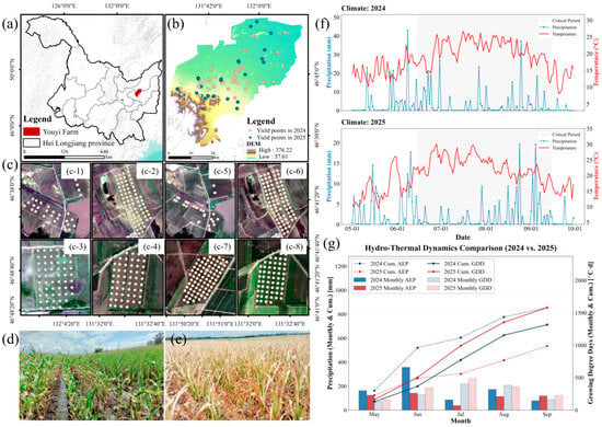
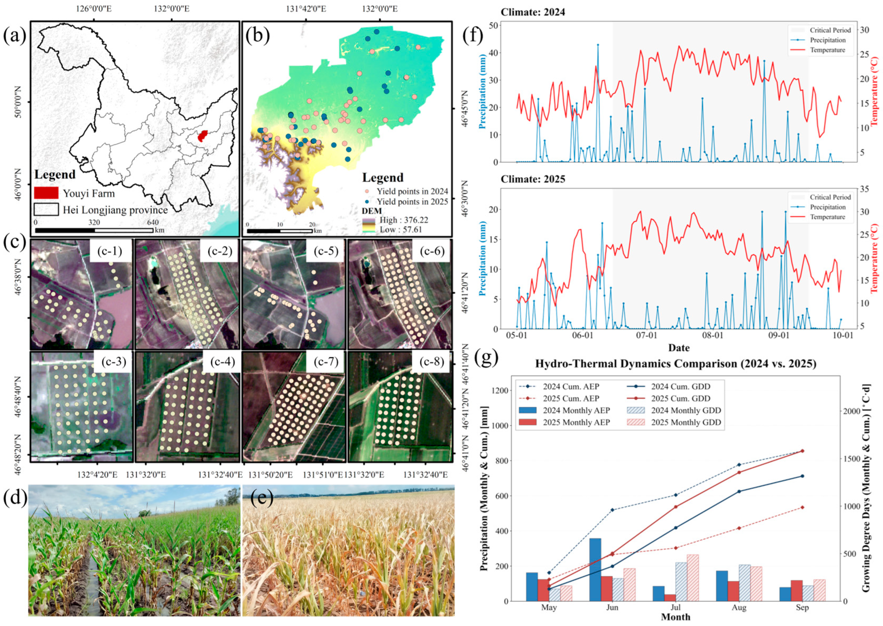
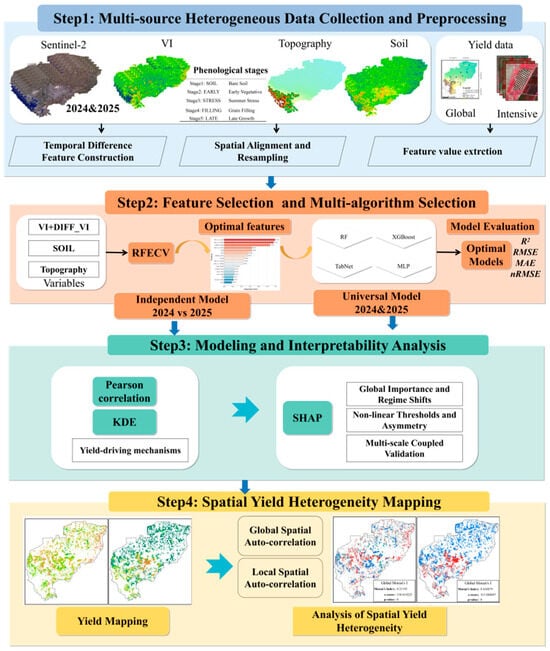
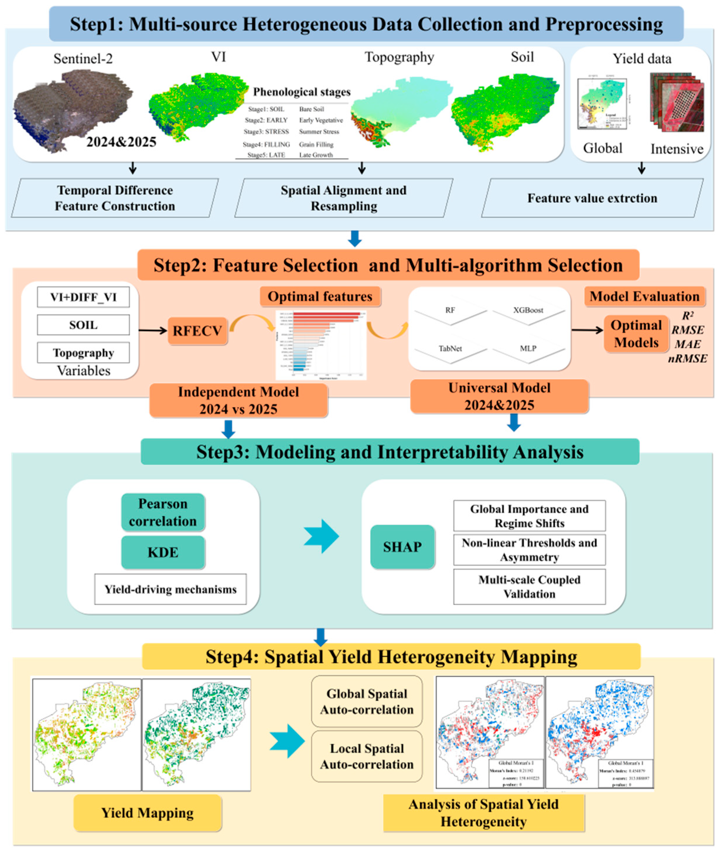
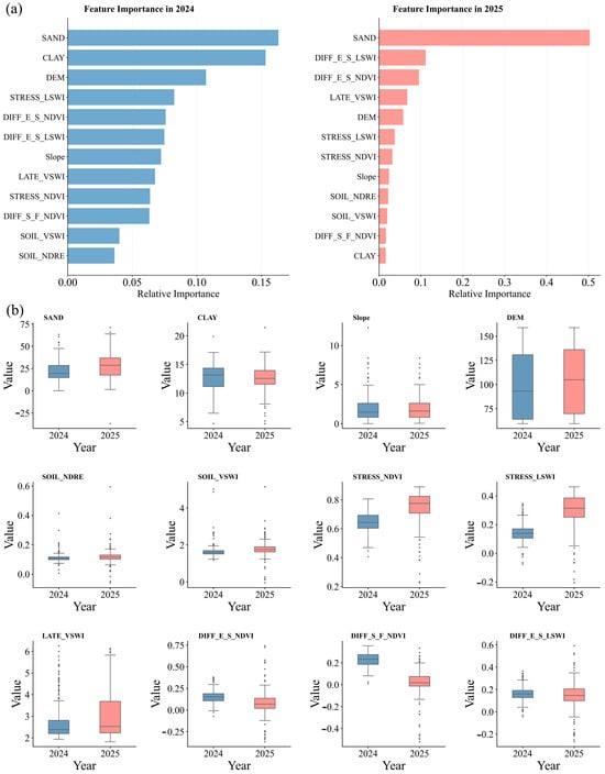
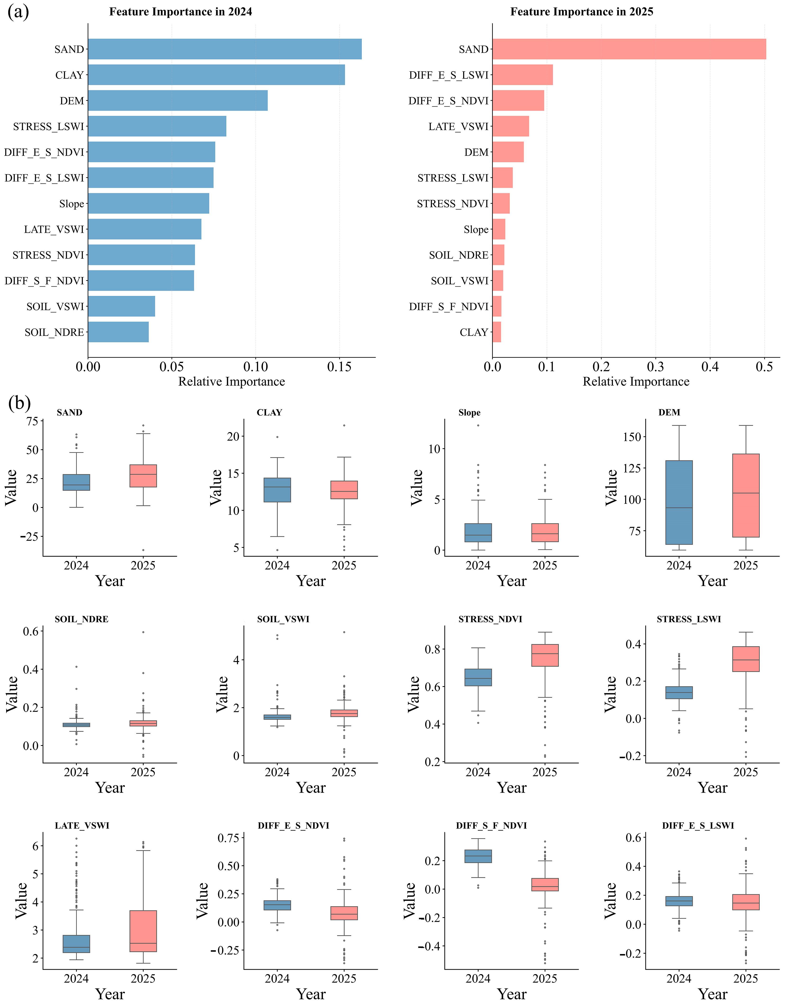
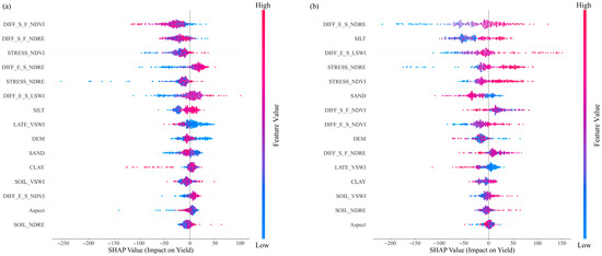
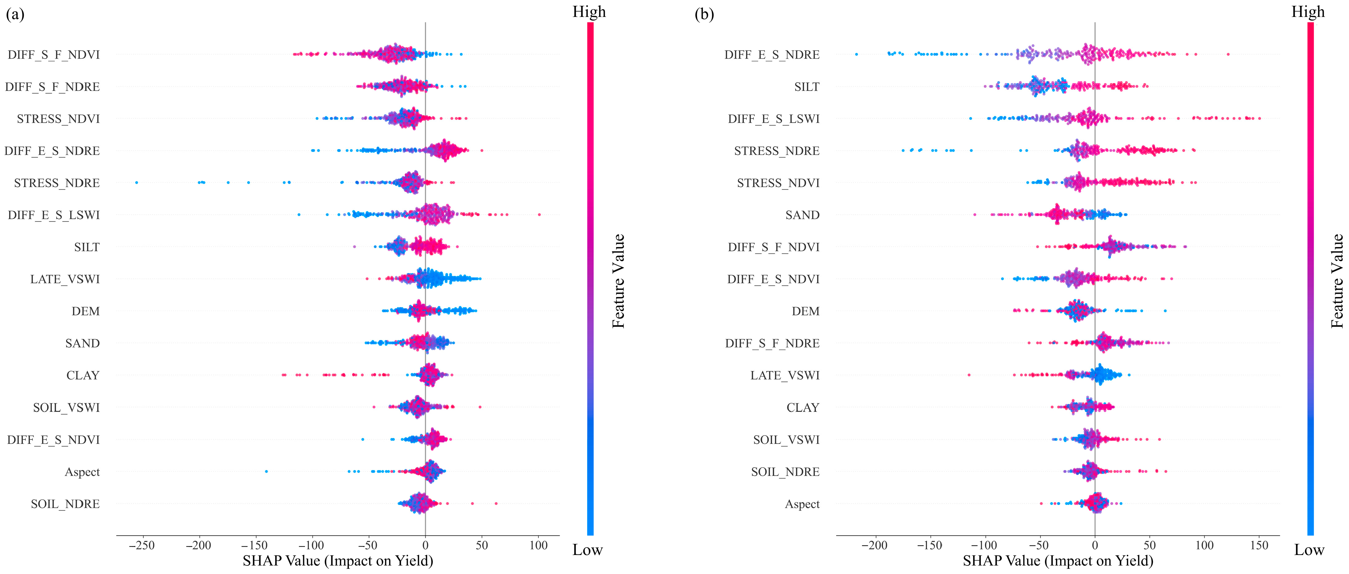
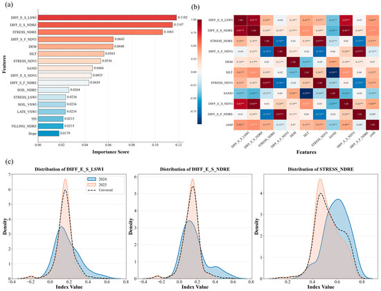
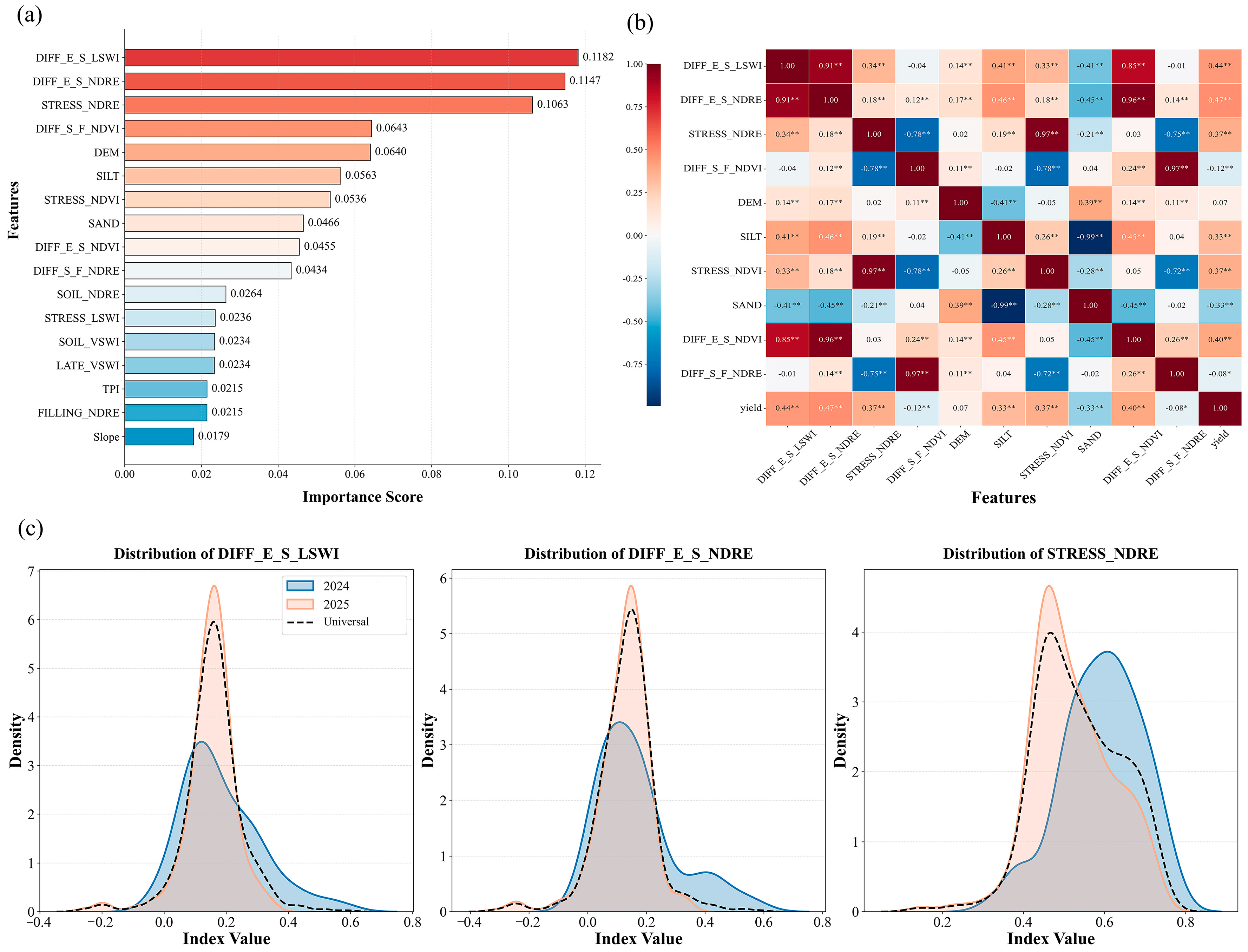
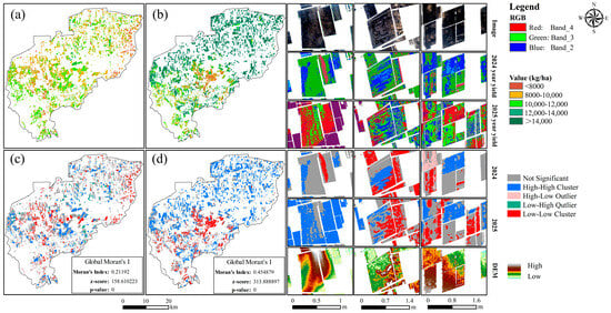
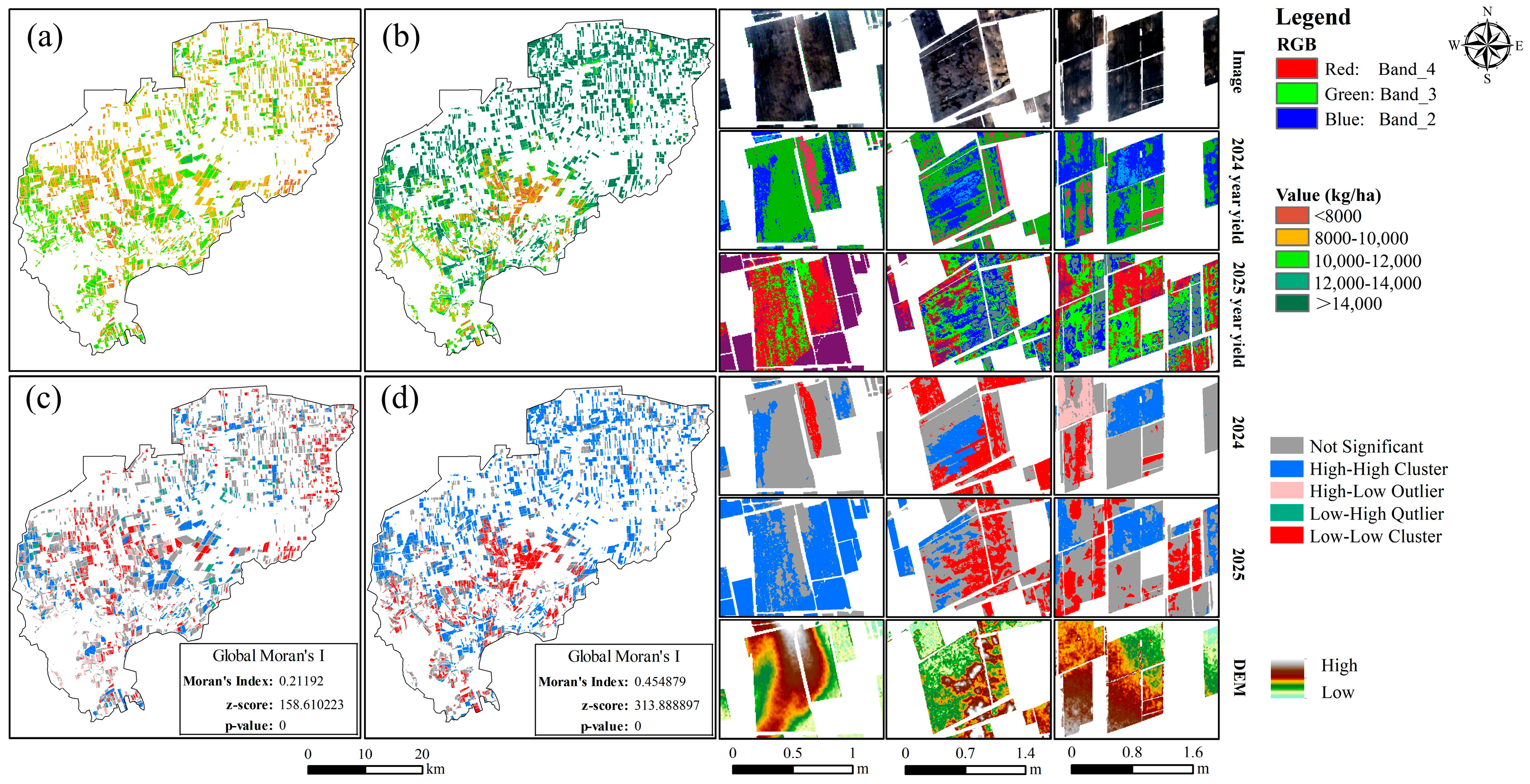
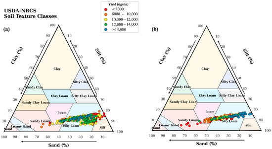
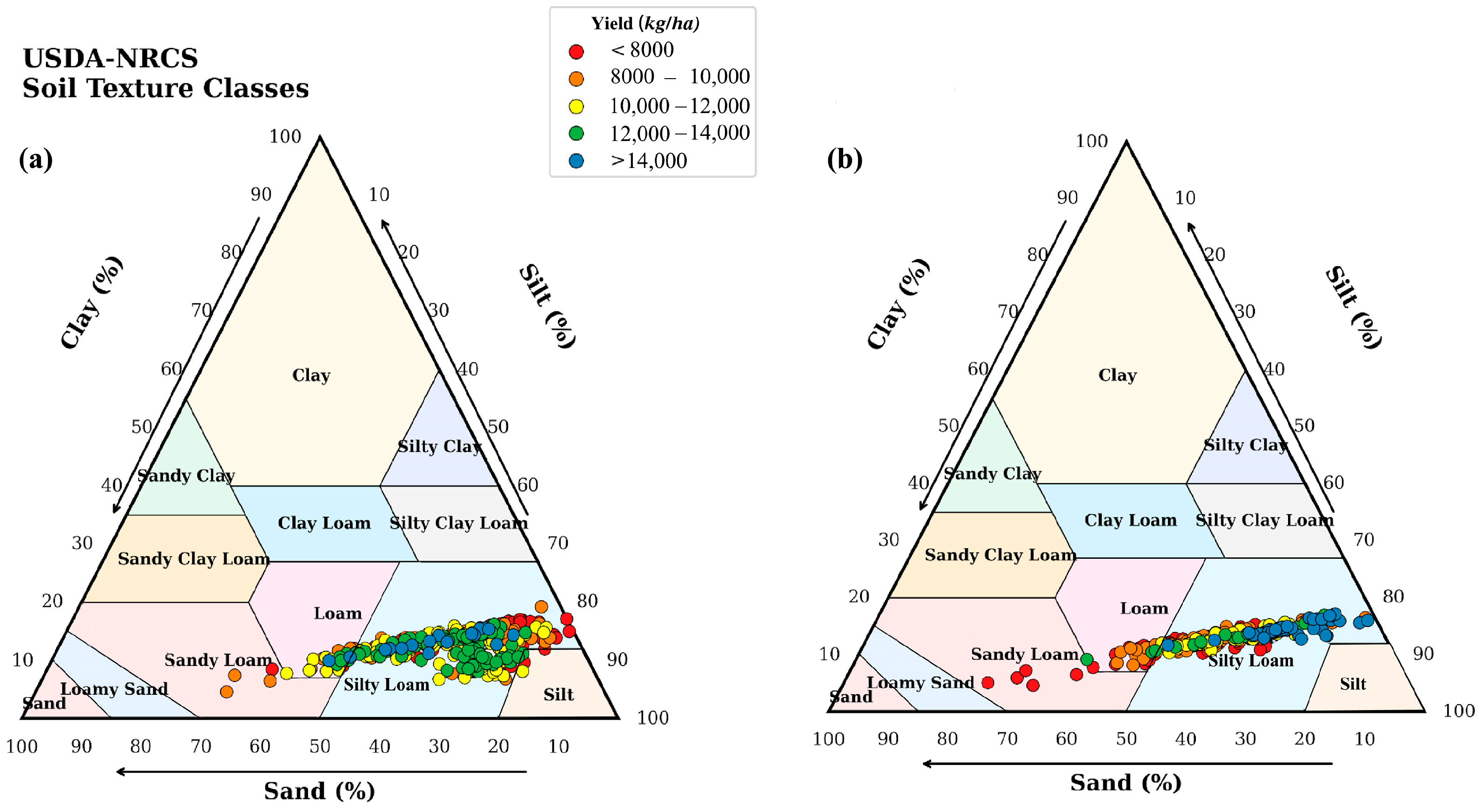
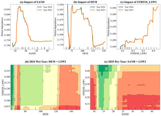
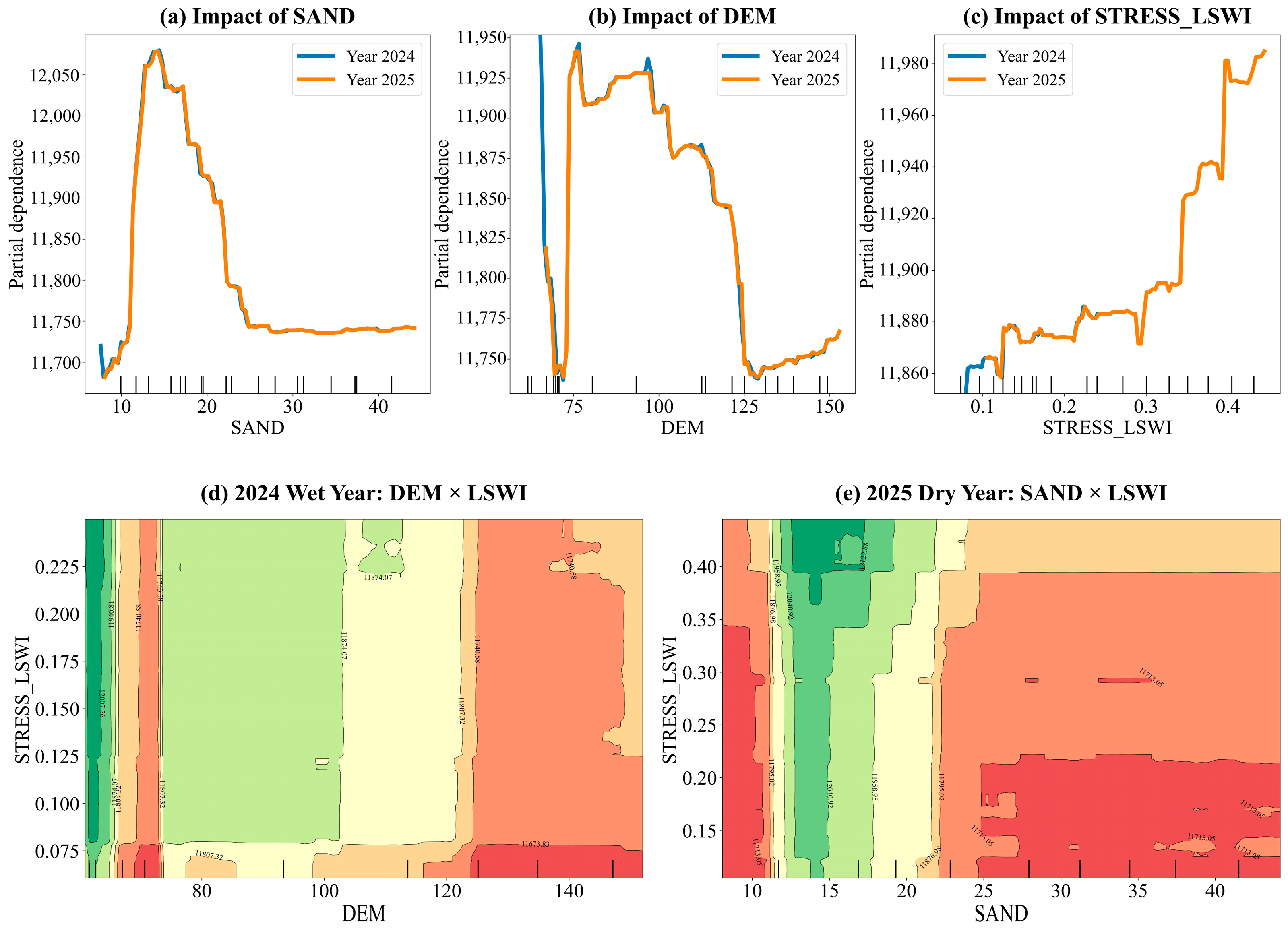
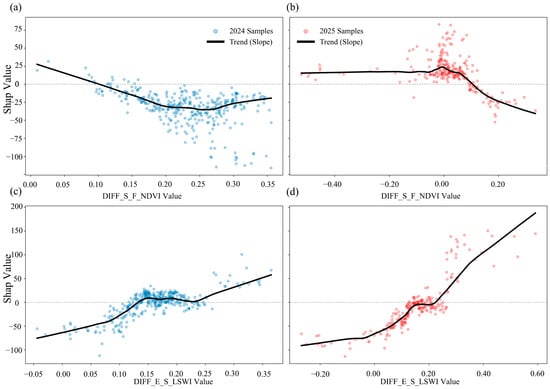
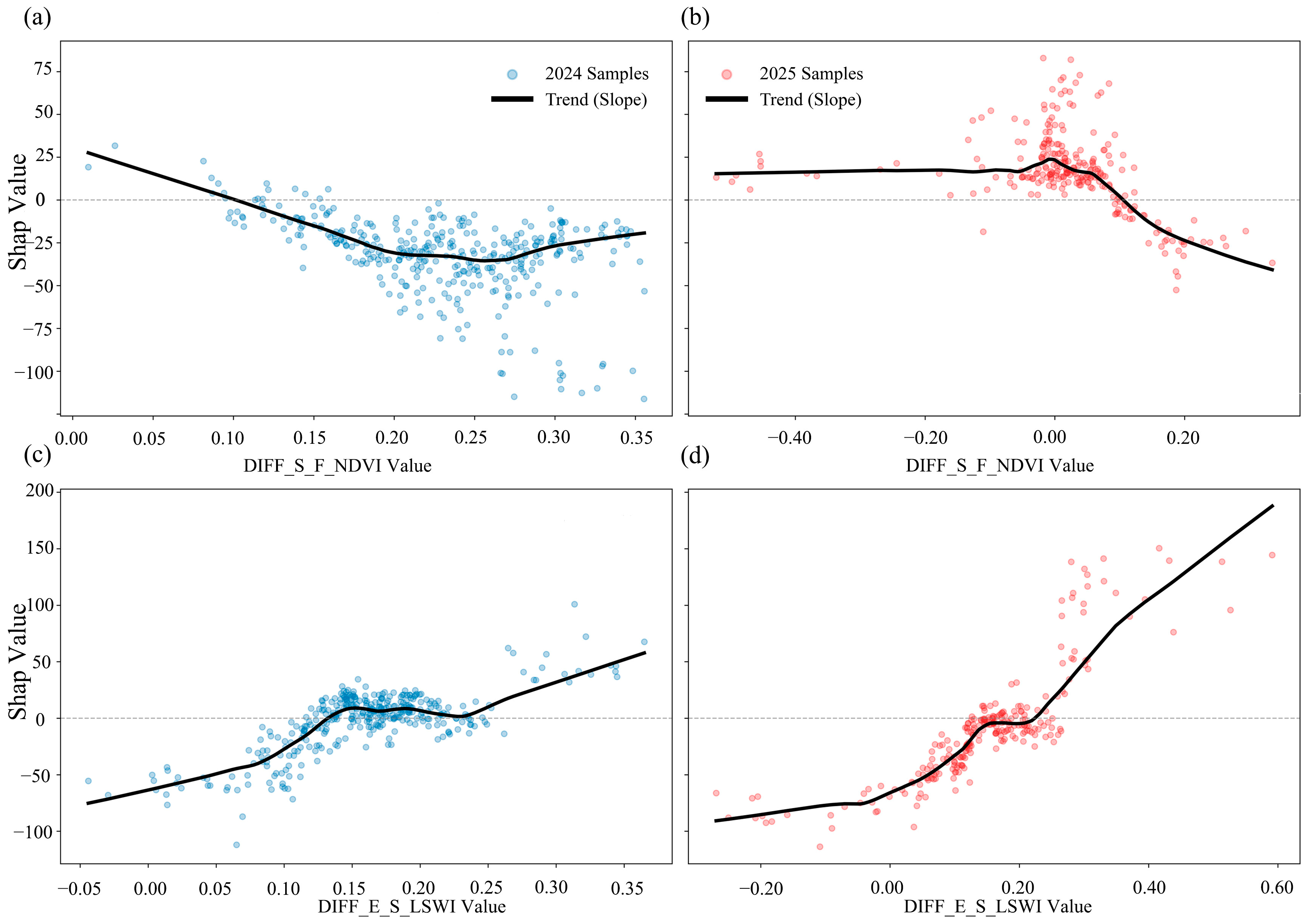
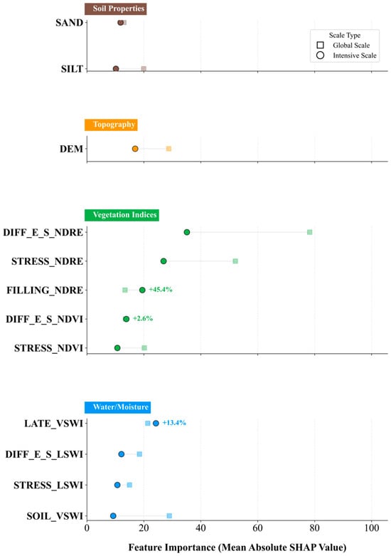
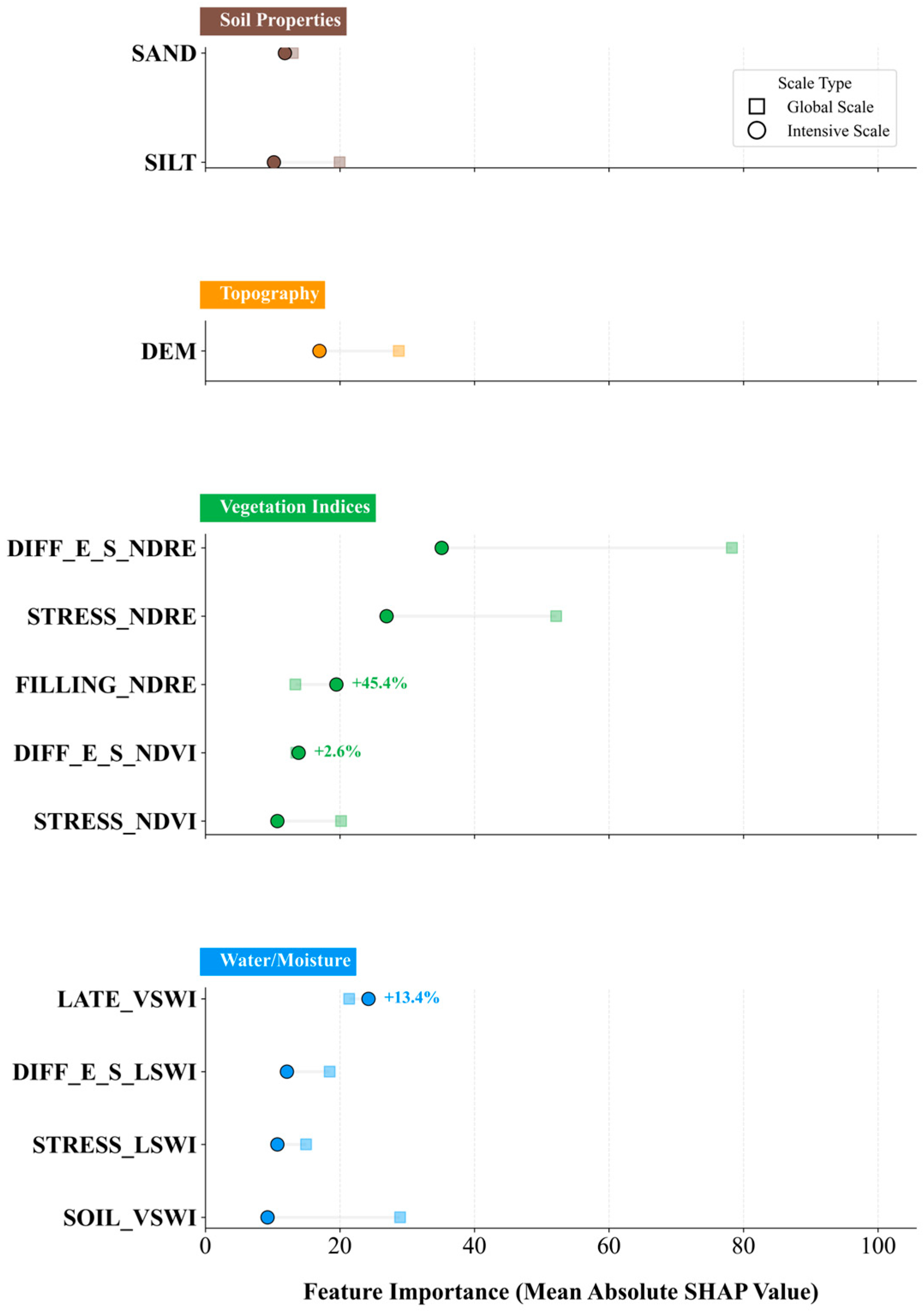

Disclaimer/Publisher’s Note: The statements, opinions and data contained in all publications are solely those of the individual author(s) and contributor(s) and not of MDPI and/or the editor(s). MDPI and/or the editor(s) disclaim responsibility for any injury to people or property resulting from any ideas, methods, instructions or products referred to in the content. |
© 2026 by the authors. Licensee MDPI, Basel, Switzerland. This article is an open access article distributed under the terms and conditions of the Creative Commons Attribution (CC BY) license.