


Abstract
To address escalating natural and market risks in agriculture, integrated crop–livestock systems (ICLS) are increasingly recognized as a production mode combining resilience and sustainability. Using survey data from 372 farm households in Inner Mongolia, China, this study first constructs a directional income volatility indicator and applies the Kruskal–Wallis test together with robust tests for equality of variances to compare the short-term risk-buffering performance of specialized cropping, specialized livestock production, and ICLS. The analysis then focuses on 190 ICLS households and employs Hansen’s threshold model to identify nonlinear constraints on achieving higher income and examine potential equipment misallocation. The results show a stronger short-term risk-buffering advantage of ICLS over the two specialized modes. Livestock inventory scale exhibits a threshold effect: at a lower livestock inventory scale, livestock expansion is significantly associated with lower income, whereas beyond this threshold the marginal effect becomes significantly positive. Crop–livestock structural matching, measured by the livestock–land ratio, constrains the income effect of livestock expansion: once the ratio reaches a certain level, livestock expansion no longer shows a significant negative association with income. In addition, mismatches between machinery investment and production orientation weaken the income performance. These results imply that policy should promote ICLS in a context-specific and moderate manner, guide farmers toward better crop–livestock alignment, and expand agricultural service provision to reduce risks associated with misaligned mechanization.
1. Introduction
In an increasingly complex global economic and ecological context, farmers face dual exposure to natural and market risks. On the one hand, uncertainties such as climate variability, extreme weather events, and animal disease outbreaks are intensifying [1]. On the other hand, fluctuations in agricultural commodity prices and rising input costs have led to greater volatility in farm income [2]. Long-term cross-country evidence shows that agricultural households are often more exposed to income fluctuations than other types of households; such volatility not only undermines household financial resilience [3], but also affects production decisions and long-term welfare [4,5]. Accordingly, in the pursuit of green transformation and high-quality agricultural development, identifying production systems that may buffer risks while supporting income improvement has become a critical issue.
Historically, modern agricultural development has largely followed a trajectory of specialization, scale expansion, and input intensification. While this pathway has substantially improved labor productivity and output in certain sectors, it has also led to the decoupling of crop and livestock production, the disruption of nutrient cycling, increased dependence on external inputs, and the accumulation of environmental pressures [6,7,8]. Against this backdrop, integrated crop–livestock systems (ICLS), characterized by ecological recycling and production diversification, have been widely regarded as a key pathway for sustainable agricultural transformation. In terms of resource use, ICLS can enhance efficiency through material recycling and functional complementarities between crops and livestock, while reducing dependence on imported protein feed [9,10]. From an environmental perspective, ICLS reconnect soil–crop–livestock linkages, thereby potentially improving system resilience and helping mitigate trade-offs between agricultural production and environmental protection [7,11,12,13]. From a risk management perspective, even without accounting for deeper biophysical synergies, ICLS maintain a crop–livestock production portfolio that can improve the farm-level risk–return trade-off and potentially reduce downside risk [14,15,16].
However, the economic performance of integrated crop–livestock systems is subject to clear conditional constraints. First, the realization of scale economies is often constrained by high transaction costs and managerial complexity [17,18]. When integration extends beyond individual farms, the processes of partner search, contract negotiation, and enforcement generate substantial information and coordination costs [19]. At small scales, such implicit costs may substantially offset the ecological premium associated with integration. Second, the economic performance of ICLS is constrained by the degree of crop–livestock structural alignment. For diversified crop–livestock systems, higher nitrogen cycling efficiency and self-sufficiency do not necessarily correspond to higher output. If the allocation between cropping and livestock production is imbalanced, excessive emphasis on internal supply may compress absolute output, leading to a pronounced trade-off between resource-use efficiency and absolute output [12,20]. Third, mismatches between machinery investment and production structure represent a key constraint on the economic performance of ICLS [21]. Evidence from France and Brazil suggests that successful transitions—whether through input reduction or moderate intensification—depend on achieving an optimal balance between livestock demand and farm resource availability, rather than increasing machinery or chemical inputs indiscriminately [9]. Overinvestment may reduce farm-level technical efficiency, whereas appropriately scaled investments that simultaneously enhance labor productivity can improve efficiency [22,23].
In response to the widespread decoupling of crop and livestock systems in many countries [24], recoupling crop and livestock production through ICLS is regarded as an important pathway for improving resource-cycling efficiency [25]. However, whether the environmental mitigation benefits of ICLS can be translated into economic gains for farmers, and under what conditions such gains may emerge as income advantages, remains insufficiently supported by micro-level empirical evidence [26]. Specifically, three research gaps remain. First, existing studies have focused mainly on resource cycling, eco-efficiency, or environmental performance, while empirical evidence on whether ICLS can generate short-term income stability at the household level remains limited. Second, studies on the income effects of ICLS have mostly examined average income differences, with less attention to whether livestock inventory scale and crop–livestock structural matching impose nonlinear constraints on income improvement. Third, machinery asset allocation has rarely been incorporated into analyses of the economic performance of ICLS, leaving insufficient understanding of whether a mismatch between equipment investment and production focus may weaken household income effects.
Against this background, this study places the economic performance of ICLS within an integrated framework of income stability and income improvement. First, a directional income volatility indicator is constructed using net operating income from two adjacent periods to examine the short-term resilience of ICLS, namely income stability. Second, threshold effects in livestock scale and crop–livestock structure matching are identified to examine the conditions under which ICLS households may achieve higher income, namely income improvement. Building on this threshold analysis, the study further examines whether equipment mismatch is associated with income performance. This study makes three contributions. First, household-level data provide direct empirical evidence on the short-term risk-buffering advantage of ICLS. Second, the study identifies constraints on achieving higher income from the perspectives of livestock inventory scale and crop–livestock structural matching. Third, the study identifies equipment mismatch and finds that misalignment between machinery investment and production orientation is negatively associated with economic performance. Overall, this study offers a new perspective on the differentiated performance of ICLS under varying scale and structural conditions, and provides household-level evidence on income stability and income performance under increasing risk and green transition pressures.
The paper has been organized in the following way: Section 2 develops the theoretical framework and research hypotheses. Section 3 describes the study area, data sources, variable definitions, and empirical methods. Section 4 reports income-volatility comparisons across production modes, threshold regression results, and tests of equipment-allocation mismatch. Section 5 discusses the main findings in relation to the existing literature. Section 6 summarizes the main conclusions and policy implications, and outlines the originality, limitations, and future research directions of this study.
2. Theoretical Framework and Research Hypotheses
2.1. Conceptual Definitions
In this study, specialized cropping systems refer to production modes in which farm households engage exclusively in crop cultivation without undertaking livestock rearing. Production activities in such systems can be supported by well-developed agricultural service provision, whereby key operations—such as land preparation, sowing, and harvesting—are outsourced to specialized service providers [27,28].
By contrast, specialized livestock systems refer to production modes in which farm households engage exclusively in animal husbandry without undertaking crop cultivation. Production activities in such systems are carried out in relatively independent facilities and are supported by specialized equipment. Income in these systems is primarily derived from the sale of live animals or livestock products [29,30].
Integrated crop–livestock systems (ICLS) refer to production systems in which farm households simultaneously engage in crop cultivation and livestock rearing, while maintaining stable linkages of material cycling and functional complementarities between the two subsystems. Specifically, crops are primarily cultivated for human consumption, while a portion of grain and crop residues is used as livestock feed [31]. In turn, livestock manure is recycled back to cropland as a substitute for chemical fertilizers, thereby forming an internal crop–feed–livestock–manure–cropland cycle [9,32,33].
2.2. Risk-Buffering Advantages of Integrated Crop–Livestock Systems
Portfolio theory suggests that, when returns from different assets are not perfectly positively correlated, a portfolio can diversify risk through asynchronous fluctuations among income streams [34]. This logic has been introduced into agricultural diversification research to explain how diversified operations reduce farm income volatility through low-correlated income sources [35], and has been further examined in crop diversification systems and crop–livestock portfolios [36,37]. However, traditional portfolio logic mainly emphasizes risk diversification across income sources and often assumes that total portfolio income equals the simple sum of individual incomes. ICLS differ from general diversification because crop and livestock activities are connected through bioeconomic interactions, such as manure return, straw feeding, and input substitution. These interactions may generate system income beyond the simple sum of crop and livestock income, namely super-additive synergistic income. Therefore, building on the mean–variance framework of portfolio theory proposed by Markowitz (1952) [34], this study takes risk diversification as the theoretical basis for analyzing the risk-buffering advantage of ICLS. Drawing on Franzluebbers et al. (2014) [6], Bonaudo et al. (2014) [9], and Han et al. (2023) [25] on material cycling, input substitution, and circular-economy effects in ICLS, this study further introduces a synergistic income term and decomposes total household net operating income into crop net income, livestock net income, and system-level synergistic income. To provide a unified analytical framework, the total farm net income of household is defined as:
where denotes crop net income, denotes livestock net income, and denotes the contribution of internal system synergies, such as material cycling, input substitution, and functional complementarity, to net operating income. It captures the part of the portfolio benefit beyond simple income addition.
Given that agricultural production is exposed to price volatility, yield uncertainty, and natural risks, farmers do not simply maximize income; rather, they trade off expected income against income volatility. The farmer’s utility function can therefore be written as:
where denotes the coefficient of risk aversion, denotes expected net operating income, and denotes the volatility of net operating income.
On this basis, for specialized cropping households, total net operating income is , with , where denotes the variance in crop net income. For specialized livestock households, total net operating income is , with , where denotes the variance of livestock net income. For ICLS, total net operating income is , and . Thus, income volatility in ICLS is not merely the sum of crop-income and livestock-income volatility, but also depends on the correlation between the two direct income sources and the volatility of the synergistic income term . denotes the correlation coefficient between crop net income and livestock net income. When , the two income sources move perfectly together, making risk diversification difficult. When , income changes from crop and livestock activities do not fully overlap, so their combination may reduce overall income volatility. This risk-buffering effect is stronger when the correlation is close to zero or negative, as fluctuations in one activity may partially offset fluctuations in the other. This logic is consistent with the mean–variance framework of portfolio theory, in which portfolio volatility depends not only on the variance of each income source, but also on the correlation among income sources [35,36,38]. This theoretical expectation is further examined through distributional-location comparisons and robust tests for equality of variances.
Unlike the standard portfolio model, the income-stabilizing logic of ICLS also lies in the way internal resource cycling may weaken the transmission of external input-price shocks to farm profits. Let the synergistic income term be:
where denotes the intensity of manure substitution for chemical fertilizers, denotes the intensity of internal feed and crop residue use, and . Equation (3) implies that higher fertilizer prices increase the substitution value of manure, while higher feed prices enhance the benefits of internal feed and residue utilization. Therefore, through , integrated systems establish a hedging mechanism at the input level, reducing dependence on external markets and stabilizing farm income [7,39,40].
Based on this analysis, the following hypothesis is proposed:
Hypothesis 1.
Compared with specialized cropping and specialized livestock systems, ICLS are expected to exhibit lower net-income volatility.
2.3. Constraints on Income Improvement
The transition from income stability to income improvement is essentially a process in which the risk-buffering advantage of ICLS is further translated into income-generating capacity. The preceding section suggests that ICLS may reduce operational volatility through income diversification and internal resource cycling. However, stability does not automatically lead to higher income. Existing studies indicate that crop–livestock integration can improve system efficiency through input substitution, resource cycling, and production complementarity, but its implementation is also constrained by labor, capital investment, managerial attention, and organizational capacity [17]. Evidence from beef cattle farms further shows that ICLS can increase net livestock profits, but its economic effects vary across integration modes and integration intensity [41]. This implies that whether ICLS can improve income depends on whether internal net synergistic gains can be effectively released. Following the decomposition of total net operating income in Equation (1), the basic condition for income improvement in ICLS can be expressed as: . When , the synergistic gains generated by manure substitution, straw feeding, and crop–livestock complementarity are sufficient to offset the additional costs arising from integrating crop and livestock activities. Drawing on Fanchone et al. (2022) [17] on labor organization constraints in crop–livestock integration, Asai et al. (2018) [19] on coordination costs beyond farm boundaries, and Bell and Moore (2012) [37] on the development conditions of ICLS, this study summarizes the additional costs of integration as labor-organization costs, scale-related investment costs, and transaction-coordination costs:
where denotes labor organization complexity, represents livestock inventory scale, and captures transaction-coordination complexity. The parameters are the corresponding cost coefficients. In practice, both and exhibit nonlinear relationships with scale: at small scales, fixed costs and learning costs cannot be effectively spread, resulting in persistently high unit costs [42]; as scale expands, fixed costs are diluted and organizational efficiency improves through experience accumulation, leading to declining unit costs [43,44]. To further capture this nonlinearity, this study constructs a conceptual profit-increment function to describe the additional income of ICLS relative to specialized production:
where represents fixed costs associated with initial expansion, denotes the degree of crop–livestock structural matching (measured by the livestock–land ratio), captures baseline returns to scale expansion, and reflects additional synergistic gains that increase with structural matching. The term represents increasing marginal management costs as scale expands, with indicating convex cost growth. Taking the first derivative with respect to :
Equation (6) indicates that marginal returns consist of two components: (i) , capturing positive gains from scale expansion and structural matching; and (ii) , representing increasing management costs and risk pressures as scale expands. At small scales, high fixed costs, limited managerial experience, and incomplete internal cycles may result in negative incremental profits. Only when livestock scale surpasses a critical threshold does cost dilution occur and synergy effects from resource cycling begin to materialize. Setting yields the threshold scale , at which profits shift from negative to positive. This study does not directly estimate the structural parameters and , but translates this mechanism into a testable threshold-regression proposition: if the income effect of livestock inventory scale changes significantly after crossing a critical level, then scale expansion may involve a nonlinear transition from cost constraints to income realization.
However, scale expansion is not the only condition for income improvement. Existing studies show that the overall efficiency of ICLS also depends on the match between livestock inventory and land area. When this relationship is unbalanced, the overall efficiency of ICLS may fall into a “1 + 1 < 2” outcome, and an inverted U-shaped relationship may exist between the livestock–cropland ratio and overall green technical efficiency [45]. This means that if livestock scale is not matched with land carrying capacity, fodder supply, and manure-return capacity, farmers may still find it difficult to achieve synergistic gains from resource cycling and factor complementarity, even when livestock scale reaches a certain level. Based on this nonlinear logic of structural matching, this study uses a concave function to describe structural synergy:
where represents the positive synergy coefficient associated with improved structural matching, and captures the marginal constraints arising from excessive livestock density. The term reflects increasing benefits from resource cycling, while represents rising costs associated with transport, application, management, and environmental constraints when livestock density becomes excessive. Taking the derivative:
The optimal structural level is , which implies that only when structural matching reaches a sufficient level does the relationship between crop and livestock systems evolve from nominal coexistence to effective integration, thereby significantly reducing dependence on external inputs such as fertilizers and feed [15,26]. More importantly, structural matching also alters the marginal returns to scale expansion:
indicating that higher levels of structural matching amplify the marginal returns to livestock scale expansion.
In summary, this study conceptualizes the constraints on the transition from income stability to income improvement at two levels. The first is whether livestock-scale expansion can cross the scale threshold formed by fixed investment, learning costs, and management costs. The second is whether livestock scale is effectively matched with land resources, fodder supply, and manure-absorption capacity. Accordingly, the following hypotheses are proposed:
Hypothesis 2.
Livestock scale has a threshold effect on farm income under ICLS; once the threshold is crossed, the marginal effect shifts from negative to positive.
Hypothesis 3.
Crop–livestock structural matching exerts a moderating threshold effect on the income impact of livestock scale; when structural matching is below a critical level, livestock-scale expansion is less likely to translate into income improvement.
2.4. Equipment Mismatch and Income Performance
Given fixed scale and structural conditions, the income level of farm households engaged in ICLS further depends on the allocation efficiency of production factors across different production activities. Aragón et al. (2024) [46] and Adamopoulos et al. (2022) [47] show that when production factors such as capital, land, and labor fail to flow to uses with higher marginal returns, overall production efficiency and income are suppressed. Zmyślona et al. (2024) [22] further notes that more agricultural capital investment is not always better; when investment does not match farm scale, labor allocation, or production structure, overinvestment may reduce technical efficiency. Based on this logic, this study decomposes total household capital into crop machinery capital and livestock-specific capital:
where denotes capital invested in cropping machinery, and denotes livestock-specific capital. This decomposition is a theoretical treatment based on the capital allocation characteristics of ICLS households, aiming to distinguish the two types of machinery capital in terms of production use, asset attributes, and substitutability. Further, let represent the household’s production orientation. When the household’s production focus is oriented toward cropping, a higher share of crop machinery capital may be reasonable. When the production focus shifts toward livestock, capital allocation should also shift toward livestock facilities, forage processing, manure treatment, and housing equipment. Therefore, this study assumes an optimal capital ratio consistent with production orientation:
Drawing on the resource misallocation literature, which characterizes efficiency losses through deviations of factor allocation from efficient states [46,47], the degree of resource misallocation is defined as:
where indicates perfect alignment, and larger values of imply more severe deviations between capital allocation and production orientation. To capture the profit erosion caused by resource misallocation, is incorporated into the profit function:
where denotes potential profit after accounting for scale and structural effects, captures efficiency losses induced by resource misallocation, and represents depreciation and sunk costs arising from underutilized cropping machinery, with denoting the utilization rate. Livestock-related capital typically exhibits strong asset specificity and is closely tied to livestock production, making it less likely to become idle as long as livestock activities continue. In contrast, cropping machinery tends to be more general-purpose and more easily substitutable through external agricultural service provision [27]. When production orientation shifts toward livestock while substantial cropping machinery is still retained, low utilization rates and high depreciation costs can directly offset the gains from livestock expansion. From the perspective of resource misallocation, capital that fails to flow toward higher marginal-return uses leads to a reduction in overall efficiency [46,47]. From the perspective of asset specificity, capital with lower specificity and higher substitutability is more likely to become sunk when production orientation shifts [48,49].
Based on the analysis, the following hypothesis is proposed:
Hypothesis 4.
Misalignment between machinery investment and production orientation significantly weakens income performance.
3. Materials and Methods
3.1. Study Area
This study selects two prefecture-level cities in central and western Inner Mongolia as the survey areas, taking into account regional resource endowments and agricultural production characteristics (Figure 1). The first is Bayannur, located in the “Golden Crop Belt,” where favorable combinations of soil, water, light, and thermal conditions support high agricultural productivity. It represents a resource-endowed agro-pastoral transitional zone [50]. The second is Ulanqab, characterized by complex terrain and a continental monsoon climate, with concentrated precipitation and relatively fragile ecological conditions. It represents an agro-pastoral transitional zone constrained by ecological limitations and climate sensitivity [51]. Both areas are typical agro-pastoral transition zones where cropping and livestock production coexist and farming modes are diverse, thereby meeting the sample requirements for comparing risk performance across production modes and further examining the income mechanisms of ICLS households. In addition, the joint inclusion of Bayannur and Ulanqab allows the analysis to cover two representative production contexts: irrigated high-yield farming and hilly dryland farming. Such a two-site design improves the explanatory relevance of the findings for regions with different resource endowments and production conditions.
Figure 1.
Study areas in Inner Mongolia, China. (a) Geographic location of Inner Mongolia within China; (b) Location of Bayannur and Ulanqab within Inner Mongolia; (c) Spatial distribution and elevation of sampled county in Ulanqab; (d) Spatial distribution and elevation of sampled counties in Bayannur. The figure was created using QGIS 3.44.7-Solothurn.
Field data were collected between August and November 2024 using a multi-stage stratified random sampling approach. In the sampling process, three counties (Hangjinhou Banner, Urad Front Banner, and Wuyuan County) were selected in Bayannur, and Huade County was selected in Ulanqab. Within these counties, townships and administrative villages were further sampled, and farmers were surveyed through face-to-face structured interviews (see Figure 1).
A total of 400 questionnaires were distributed, including 320 in Bayannur (123 in Hangjinhou Banner, 100 in Urad Front Banner, and 97 in Wuyuan County) and 80 in Huade County, Ulanqab. After excluding observations with missing key information, logical inconsistencies, or extreme outliers, 372 valid samples were retained, yielding an effective response rate of 93.0%. Based on actual production modes, the final sample consists of 190 households adopting integrated crop–livestock systems, 170 households engaged in specialized cropping, and 12 households engaged in specialized livestock production.
3.2. Variable Measurement and Definition
3.2.1. Explained Variables
In line with the study objectives, two core explained variables are constructed. The first captures the risk-buffering capacity of different production modes using a directional income volatility indicator. The second is the inverse hyperbolic sine (IHS) transformation of two-year average net farm income, which is used to examine the constraints on achieving higher income among ICLS households. It should be noted that all variable calculations and statistical analyses were performed using Stata 18.0.
- Directional Income Volatility
To accurately assess the risk-buffering capacity of specialized cropping, specialized livestock, and integrated crop–livestock systems, this study constructs a directional income volatility indicator as the primary explained variable. It is defined as the difference in inverse hyperbolic sine (IHS)-transformed net farm income between 2023 and 2022:
where and denote the net farm income of household in 2023 and 2022, respectively. The inverse hyperbolic sine transformation is defined as:
where represents the original income variable.
Compared with commonly used risk measures, the directional income volatility indicator developed in this study has three main advantages. First, variance, standard deviation, and the coefficient of variation describe the dispersion of income around the mean, but cannot distinguish the direction of income change. The focus of this study is to identify which production mode is less likely to experience income decline under external shocks. By retaining positive and negative signs, the directional income volatility indicator directly distinguishes upward income improvement from downward income deterioration. Second, the conventional income growth rate contains directional information, but becomes undefined when baseline income is zero or negative and remains sensitive to extreme values. The IHS transformation, by contrast, is defined over the entire real domain, applies to variables with positive, zero, and negative values, and reduces the influence of extreme observations [52]. Moreover, when variable values are large, the IHS transformation approximates the logarithmic transformation. Therefore, the IHS difference in two-period net income is economically close to a log difference and reflects the relative magnitude of income change [53]. Third, compared with downside-risk measures such as semivariance, the directional income volatility indicator places greater emphasis on identifying the direction of income change. Semivariance mainly captures downward deviations below a given benchmark [54]. By contrast, the IHS difference retains the sign of income changes between two adjacent periods and directly distinguishes income increases from income declines. Therefore, the IHS-based directional indicator is more consistent with the analytical focus on short-term operational stability and downside-risk exposure.
- 2.
- IHS-Transformed Average Net Operating Income
To examine the constraints on achieving higher income in ICLS, the average net operating income over two periods is used as the core explained variable and transformed using the inverse hyperbolic sine (IHS) function. The specific formulation is given by:
The explained variable is measured as two-year average net income because averaging income over two years helps smooth short-term fluctuations and better reflects the household’s regular operating income level.
Regarding functional form, the IHS transformation is adopted for three reasons. First, using untransformed net operating income may make model estimates sensitive to right-skewed income distributions and extreme observations, allowing a small number of high-income or loss-making households to exert disproportionate influence on the results. Second, the natural logarithmic transformation, , can compress right-skewed distributions and extreme values, but requires y > 0 and cannot handle zero or negative net operating income. The shifted logarithmic transformation, extends the variable domain, but the choice of the constant is partly arbitrary and may affect variable scaling and estimation results. Third, the Box–Cox transformation provides a more flexible functional form, but the standard Box–Cox transformation also requires positive values. When a shift parameter is used to handle non-positive values, additional parameter selection or estimation remains necessary, and coefficient interpretation becomes more dependent on the chosen transformation parameters [53]. By comparison, the IHS transformation retains positive, zero, and negative income observations, requires no artificially specified shift constant, and reduces the influence of extreme values through a log-like compression feature [52]. Therefore, given the right-skewed distribution, extreme observations, and zero and negative values in household net operating income, IHS-transformed average net operating income provides an appropriate dependent-variable specification.
3.2.2. Explanatory Variables
Existing studies suggest that farm household income and production decisions are jointly influenced by five capitals, including natural, physical, financial, social, and human capital [14,16,55]. Accordingly, core explanatory variables and control variables are selected from these five dimensions, including livestock inventory scale, operated land area, machinery asset value, household debt, cooperation participation, and the household head’s age, education, and health status. In addition, the livestock–land ratio is introduced to capture the degree of crop–livestock structural matching and to examine whether structural matching affects the income effect of livestock inventory expansion. Definitions and measurements of all variables are reported in Table 1.
Table 1.
Definition and measurement of explanatory variables.
When incorporating livestock inventory scale into the analysis, differences across livestock species in body size, metabolic rate, feed consumption, and manure emissions need to be accounted for. To ensure comparability, this study adopts a pig-equivalent conversion approach to standardize livestock units across species [56]. The pig-equivalent unit is widely used in the measurement of livestock-related pollution and production scale in agricultural studies. One pig is defined as one pig-equivalent unit. Following official guidelines issued by the Ministry of Agriculture and Rural Affairs of China [57], and local livestock conversion standards [58], the pig-equivalent coefficients for adult animals are set as follows: pigs = 1; cattle = 3.33; sheep = 0.40; poultry = 0.04; and donkeys = 3.00.
The above official conversion standards primarily apply to adult livestock. However, farmers typically raise both adult and young animals simultaneously. To account for differences in resource use and emissions across growth stages, this study further adjusts pig-equivalent coefficients for young livestock based on biological scaling principles. Specifically, following Kleiber’s law [59,60], which states that an animal’s basal metabolic rate scales with body mass to the power of 3/4, the pig-equivalent coefficient for young livestock is defined as:
where denotes the pig-equivalent coefficient for adult livestock of species , and and represent the average body weights of young and adult animals, respectively.
Based on the above adjustments, the composite livestock inventory scale indicator is constructed as:
where and denote the numbers of adult and young livestock of species raised by household , respectively. Finally, the livestock inventory scale variable is defined as the average pig-equivalent value over 2022 and 2023, which helps reduce the influence of short-term fluctuations in scale measurement.
3.3. Methods
3.3.1. Kruskal–Wallis Nonparametric Test
To identify differences in the overall distribution of the directional income volatility indicator across production modes, this study employs the Kruskal–Wallis nonparametric test for an overall comparison. Because the directional income volatility indicator constructed in this study may exhibit substantial skewness or contain extreme values, it does not necessarily satisfy the strict assumptions of normality and homoscedasticity required by parametric tests. To address this limitation, we adopt the rank-based Kruskal–Wallis procedure [61]. The basic idea of this method is to pool and rank all observations across groups, replace the original values with their ranks, and then test whether the rank sums differ systematically across groups. This procedure requires that samples be mutually independent and that the population distributions have broadly similar shapes, but it does not require the data to follow a normal distribution, making it suitable for the directional income volatility indicator constructed in this study.
Formally, suppose the full sample is divided into independent groups, with group containing observations, and total sample size . After ranking all observations jointly, let denote the sum of ranks in group . The Kruskal–Wallis statistic is then given by:
When tied observations are present, average ranks are assigned and a tie correction is applied. The corrected statistic is:
where , and denotes the number of observations sharing the same value within a given tie group. is the sum of tie-correction terms across all tie groups. Under the null hypothesis and for sufficiently large sample sizes, the corrected statistic approximately follows a chi-square distribution with degrees of freedom, that is, .
3.3.2. Tests for Equality of Variances
Given the unequal sample sizes across the three production modes, this study adopts robust tests for equality of variances to compare the dispersion of income volatility indicators across groups [62]. Formally, let denote the -th observation in group , where correspond to specialized cropping, integrated crop–livestock systems, and specialized livestock, respectively. Let denote a measure of central tendency for group . The absolute deviation is defined as:
where can be specified as the group mean, group median, or trimmed mean [63]. Subsequently, a test for equality of variances is conducted based on . If the mean absolute deviations differ significantly across groups, this indicates that the variances of the original variable are not equal. The null hypothesis is , while the alternative hypothesis is that at least one group differs.
3.3.3. Regression Models
To examine the determinants and mechanisms of average net operating income among ICLS households, this study specifies an OLS model, two threshold regression models, and a moderation model. To ensure consistency with the model numbering in the empirical results, the models are specified as follows.
Let denote the IHS−transformed two-year average net operating income of ICLS household , denote livestock inventory scale, denote the livestock–land ratio, denote a vector of control variables, denote the error term, denote the constant term, and denote the vector of coefficients for the control variables.
Model 1 examines the overall linear effect of livestock inventory scale on average net operating income and serves as the baseline for the subsequent threshold and mechanism models:
In Equation (22), captures the overall marginal effect of livestock inventory scale on average net operating income.
Model 2 tests whether the income effect of livestock inventory scale differs across scale regimes. Taking as the threshold variable, the livestock-scale threshold model is specified as:
where is an indicator function equal to 1 when the condition holds and 0 otherwise. and denote the marginal effects of livestock inventory scale below and above the threshold value , respectively. The threshold value is endogenously estimated from the sample data [64]. Specifically, households are first sorted by the threshold variable, and the extreme observations at both tails are trimmed at 10% to ensure sufficient observations on both sides of the threshold. The remaining values of are then used as candidate thresholds. For each candidate threshold, a segmented regression is estimated and the residual sum of squares is calculated. The candidate value that minimizes the residual sum of squares is selected as the estimated threshold . Finally, a Wald test is used to examine whether the coefficients of livestock inventory scale differ across threshold regimes. Rejection of the null hypothesis indicates a significant difference in the income effect of livestock inventory scale before and after the threshold [65].
Model 3 examines whether the marginal effect of livestock inventory scale differs across livestock–land ratio regimes. Taking as the threshold variable, the structural-matching threshold model is specified as:
where is the endogenously estimated threshold value of the livestock–land ratio, and and denote the marginal effects of livestock inventory scale in the low- and high-ratio regimes, respectively.
To identify the income effect of mismatch between equipment allocation and production structure, machinery assets are divided into crop machinery and livestock machinery . The livestock–land ratio is introduced as a moderator reflecting production structure. Model 4 includes only the main effects:
where , , and capture the direct effects of crop machinery, livestock machinery, and the livestock–land ratio on average net operating income, respectively.
Model 5 adds interaction terms between machinery assets and the livestock–land ratio to test whether production structure moderates the income effects of machinery assets:
In Equation (26), captures the moderating effect of the livestock–land ratio on the income effect of crop machinery, while captures the corresponding moderating effect on the income effect of livestock machinery.
4. Results
4.1. Comparison of Risk-Buffering Capacity Across Production Modes
4.1.1. Distributional Characteristics of Directional Income Volatility
Before conducting formal statistical inference, this study provides a preliminary assessment of the distributional characteristics of income volatility across production modes by combining descriptive statistics (Table 2) with kernel density estimates (Figure 2). Two main findings can be identified. First, in terms of dispersion, integrated crop–livestock systems (ICLS) exhibit greater income stability. As shown in Table 2, the standard deviation is lowest for ICLS, followed by specialized cropping systems, while specialized livestock systems display the highest variability. The kernel density plots in Figure 2 further support this finding: the distribution for ICLS is more concentrated and peaks more sharply around zero, indicating relatively stable intertemporal income changes. In contrast, the distribution for specialized livestock systems is flatter and more dispersed, with more pronounced tails, suggesting greater income fluctuations and weaker overall stability. Second, regarding distributional shape, the income volatility indicators for all three production modes exhibit clear non-normal characteristics. As reported in Table 2, kurtosis values substantially exceed the benchmark value of 3 for a normal distribution, and skewness deviates from zero. Figure 2 also visually confirms the presence of leptokurtic distributions with heavy tails. These distributional features provide empirical support for the use of nonparametric methods in subsequent analysis.
Table 2.
Descriptive statistics of directional income volatility across production modes.
Figure 2.
Kernel density estimates of directional income volatility across production modes.
4.1.2. Distributional Location Comparison Across Production Modes
Given that the directional income volatility indicator does not satisfy the normality assumption, the Kruskal–Wallis test is used to compare distributional locations across the three production modes. Table 3 reports a Kruskal–Wallis overall test statistic of 8.504, with a p-value of 0.0142 (<0.05), indicating significant overall differences in directional income volatility across production modes. To further identify the source of these differences, pairwise Wilcoxon rank-sum tests are conducted. Since three pairwise comparisons are performed, the Bonferroni correction is applied to control for multiple testing [66], with the adjusted significance threshold set at 0.0167 (0.05/3). Under this threshold, the difference between specialized cropping and ICLS remains significant. By contrast, the comparison between specialized cropping and specialized livestock production yields a p-value of 0.1874, while the comparison between ICLS and specialized livestock production yields a p-value of 0.4405; neither comparison reaches statistical significance.
Table 3.
Kruskal–Wallis test and pairwise comparisons of directional income volatility.
Because the directional income volatility indicator retains positive and negative signs, differences in distributional location across production modes can also indicate whether income changes are more likely to be positive or negative. Given the comparison order in Table 3, the negative Wilcoxon statistic for specialized cropping versus ICLS (z = −2.760) indicates that specialized cropping has lower ranks and a more left-shifted distribution than ICLS. This finding is consistent with the kernel density pattern in Figure 2, suggesting that, compared with specialized cropping, ICLS shows a lower tendency toward negative income changes.
4.1.3. Tests for Equality of Variances Across Production Modes
To examine whether the dispersion of directional income volatility differs significantly across production modes, this study employs robust tests for equality of variances, implemented using the robvar command in Stata [67]. Specifically, the test statistics include W0, corresponding to Levene’s test, as well as two robust Brown-Forsythe variants, namely W50 and W10. The latter two adopt more robust measures of central tendency—based on the median and the 10% trimmed mean, respectively—making them less sensitive to skewed distributions and extreme values, and therefore more suitable for the distributional characteristics of the directional income volatility indicator used in this study.
The overall test results in Table 4 indicate that the variances of directional income volatility differ significantly across production modes. Further pairwise robust comparisons show that the dispersion differs significantly between specialized cropping and ICLS, as well as between ICLS and specialized livestock systems, whereas the difference between specialized cropping and specialized livestock systems is not statistically significant. Combined with the descriptive statistics reported in Table 2, it can be observed that integrated crop–livestock households exhibit the lowest standard deviation of directional income volatility (SD = 8.081), followed by specialized cropping (SD = 9.337), while specialized livestock systems display the highest variability (SD = 14.187). These findings indicate that the dispersion of income volatility under integrated crop–livestock systems is significantly lower than that of specialized livestock systems and, to some extent, lower than that of specialized cropping systems. Given that values of directional income volatility closer to zero imply more stable intertemporal income changes, a lower dispersion indicates that observations are more concentrated around zero, reflecting smoother income fluctuations. Taken together, the distributional location comparisons and robust variance tests suggest that ICLS have a stronger risk-buffering advantage in both the direction and stability of income changes. Therefore, H1 is supported.
Table 4.
Robust tests for equality of variance in directional income volatility by production modes.
4.1.4. Robustness Test for the Risk-Buffering Performance of ICLS
To address potential self-selection bias arising from differences in farmers’ initial conditions, this study applies inverse probability weighting (IPW) as a robustness test [68]. IPW requires sufficient common support and stable propensity-score estimation. Because the specialized livestock group includes only 12 households, using this group as a weighted control group may generate unstable propensity scores, extreme weights, and poor covariate balance. Therefore, the IPW robustness test focuses on the more balanced comparison between 190 ICLS households and 170 specialized cropping households.
Covariates in the propensity-score model are selected based on the household livelihood capital framework and remain consistent with the variable definitions in Table 1. To reduce the influence of extreme values and skewed distributions, skewed continuous variables, such as operated land area, are winsorized at the 1st and 99th percentiles and transformed using . The household head’s age, education, health status, and cooperative participation retain their original forms. Livestock inventory scale is excluded from the propensity-score model because it is a defining production feature distinguishing ICLS from specialized cropping. Including this variable would treat the production-mode difference itself as a control condition and weaken the interpretation of self-selection adjustment.
For outcome variables, the IPW analysis does not replace the directional income volatility indicator used above. Instead, two alternative risk measures are constructed: an income-decline dummy variable and a symmetric relative income volatility indicator. The former captures whether households experience negative income changes, while the latter captures the relative magnitude of income fluctuations [69]. Variable definitions and calculations are reported in Panel A of Table 5.
Table 5.
Robustness test for the short time risk-buffering performance of ICLS.
4.2. Constraints on Income Improvement in Integrated Crop–Livestock Systems
4.2.1. Sample Characteristics of Integrated Crop–Livestock Households
Based on Table 6, the individual characteristics of household heads reveal that males account for an overwhelming majority of the sample. This pronounced gender imbalance is closely associated with traditional divisions of labor in rural China, where the norm of “men managing external affairs and women managing internal affairs” remains deeply rooted. As a result, men are typically regarded as the primary decision-makers in household production and economic activities. In addition, due to long-standing institutional practices in the rural household registration system, the household head is often officially registered as the eldest male. In terms of age structure, the main operators of ICLS are predominantly middle-aged and older farmers. On the one hand, those older farmers generally possess extensive farming experience and are more familiar with the coordination between crop cultivation and livestock production, including seasonal arrangements and resource recycling. On the other hand, this pattern reflects broader demographic trends in rural China, particularly labor aging and rural depopulation. With respect to education, most household heads have completed only compulsory education, indicating a relatively low overall level of formal schooling. In terms of health status, the sample households are generally in good physical condition.
Table 6.
Sample characteristics of integrated crop–livestock households (N = 190).
With regard to household production characteristics, the sample exhibits clear stratification in both livestock inventory scale and operated land area. Most households maintain a livestock inventory below 30 pig equivalents, and 54.74% operate less than 5 hectares of land. This indicates that integrated crop–livestock households in the study area are still predominantly small- to medium-scale operators, with substantial heterogeneity in livestock investment intensity across households. As shown in Table 5, there is also considerable variation in the total value of machinery, suggesting heterogeneity in fixed asset endowment. It should be noted that the total value of machinery does not necessarily reflect the actual level of access to mechanized services; rather, it primarily captures differences in capital investment and asset accumulation. In terms of household debt, most households have relatively low debt levels, with the majority owing less than CNY 10,000, while 25.79% report debts exceeding CNY 100,000. This suggests that the sample includes both relatively conservative households with limited capital investment and those relying on external financing to support larger-scale operations. Overall, most households operate on a relatively dispersed and small-scale basis, with a limited degree of organizational integration. In terms of economic outcomes, the majority of households fall within the CNY 0–100,000 income range, while 18.42% report non-positive average net operating income over the two-year period, and only 11.58% exceed CNY 200,000. Taken together, these results indicate that the income distribution of sample households is characterized by a predominance of low-income groups and a relatively small proportion of high-income households.
4.2.2. Baseline Regression Analysis
Table 7 reports the baseline regression results. To examine potential multicollinearity, variance inflation factors (VIFs) are calculated for all explanatory variables in the model (Appendix A Table A1). The VIF values range from 1.03 to 1.44, indicating no serious multicollinearity in the baseline specification.
Table 7.
Baseline regression results for integrated crop–livestock households.
Model 1 shows several positive associations with household net operating income. Operated land area is positive and significant at the 1% level, suggesting scale-related income gains from larger cultivated area. Cooperation participation is also significantly positive, indicating higher average net operating income among households involved in external cooperation. The household head’s health status shows a significant positive association with income, highlighting the role of physical capacity in labor-intensive agricultural production.
Livestock inventory scale shows a significant negative association with household net operating income at the 1% level. In the full-sample linear specification, livestock expansion is associated with lower net income among ICLS households. This average linear effect does not imply income suppression across all scale ranges. Combined with the theoretical analysis, the negative coefficient may reflect high fixed investment and supporting constraints during the early stage of expansion, when costs may increase faster than synergistic gains. After initial sunk costs are absorbed and standardized management is established, livestock expansion may generate positive scale effects.
To address potential reverse causality between livestock inventory scale and household net operating income, an instrumental-variable approach is further applied. IV-2SLS reports the first-stage results and endogeneity diagnostics [70], and IV-GMM provides robustness estimates after endogeneity adjustment [71]. The average livestock inventory scale of other surveyed households in the same township is used as the instrument. The instrument reflects the local livestock production base, production environment, and technology diffusion conditions, and should be correlated with household livestock inventory scale. Township-level average livestock scale is unlikely to directly determine individual household income, but may affect income indirectly through household livestock scale. The endogeneity test uses the same variable setting as Model 1 in Table 7, with all explanatory variables except livestock inventory scale included as controls.
Table 8 reports the endogeneity test results. The first-stage regression shows a significant positive effect of the instrument on household livestock inventory scale. The first-stage F-statistic is 11.032 (>10), suggesting no obvious weak-instrument problem. The endogeneity test is significant at the 10% level, indicating potential endogeneity between livestock inventory scale and household income. Because the model includes one endogenous variable and one instrument, the specification is exactly identified; therefore, IV-GMM and IV-2SLS produce identical estimates. The IV-GMM results show that livestock inventory scale remains significantly negatively associated with income after endogeneity adjustment, consistent with the baseline OLS results.
Table 8.
Endogeneity Test for Livestock Inventory Scale.
4.2.3. Threshold Effect Estimation
To identify whether the effect of livestock scale on net operating income has regime-specific characteristics, Hansen’s threshold regression model is applied to examine the marginal income effect of livestock scale from both absolute and relative scale dimensions (Table 9). Two single-threshold models are specified. The first uses livestock inventory scale as the threshold variable to identify the absolute scale threshold (Model 2, Table 9). The second uses the livestock–land ratio, measured as pig equivalents per hectare of land, as the threshold variable to examine whether the income effect of livestock inventory scale varies under different structural conditions (Model 3, Table 9).
Table 9.
Threshold regression results for scale and structural threshold effects.
From the scale dimension, Model 2 identifies a threshold value of 4.750, corresponding to approximately 115 pig equivalents. Below this threshold, livestock inventory scale is significantly negatively associated with net income; above this threshold, the association becomes significantly positive. The Wald test rejects coefficient equality across the two regimes (χ2 = 14.23, p = 0.0002), indicating a significant difference in the income association of livestock scale before and after the threshold. The additional threshold-regime diagnostic in Appendix A Table A2 identifies a lower candidate threshold of 3.257, corresponding to approximately 25 pig equivalents. However, the coefficient difference between the middle and high regimes is insignificant (χ2 = 0.12, p = 0.7318), suggesting that the three-regime specification provides no additional information beyond the two-regime model. Therefore, the more parsimonious single-threshold specification is retained.
From the structural dimension, Model 3 identifies a livestock–land ratio threshold of 18.182. Below this threshold, livestock inventory scale is significantly negatively associated with household net income; above this threshold, the negative association becomes insignificant. The regime coefficient test confirms a significant difference across regimes (χ2 = 5.02, p = 0.0251). The result suggests that livestock–land matching may shape the income association of livestock expansion. A higher livestock–land ratio may strengthen resource cycling and factor complementarity between cropping and livestock production, thereby weakening the negative income association of livestock expansion. Appendix A Table A2, however, does not further support the livestock–land ratio as an independent and stable core threshold variable. Therefore, the livestock–land ratio threshold is interpreted as supplementary evidence from the structural-matching dimension rather than core evidence comparable to the livestock-scale threshold.
Control-variable estimates are generally consistent with the baseline regression. Operated land area and household head health remain significantly positive in both threshold models. Cooperative participation also shows a positive income association, with a coefficient of 2.973 in Model 2 (p < 0.10) and 3.853 in Model 3 (p < 0.05). The stronger coefficient in Model 3 may reflect the organizational role of cooperatives in coordinating feed supply, manure return, and technical services under better crop–livestock structural matching. Machinery asset value is significantly negative in the baseline regression, but the negative coefficient becomes less significant in the two threshold models. The pattern suggests that part of the average negative association of machinery assets is absorbed after allowing livestock-scale associations to vary across regimes. Machinery-related income performance may therefore depend on the scale regime and crop–livestock matching status. The following analysis further distinguishes crop machinery from livestock machinery and examines interactions with the livestock–land ratio to identify a possible equipment-mismatch mechanism in ICLS.
For robustness, the single-threshold models are re-estimated using alternative trimming proportions. Because threshold search cannot be completed under the 5% trimming proportion due to within-regime sample size constraints, the 10% trimming proportion is used as the baseline, and the 6–14% range is used for sensitivity checks. Table 10 shows stable thresholds of 4.750 for livestock inventory scale and 18.182 for the livestock–land ratio across alternative trimming proportions. In the livestock-scale threshold model, below-threshold and above-threshold associations remain significantly negative and significantly positive, respectively, with regime differences significant at the 1% level. In the livestock–land ratio threshold model, the below-threshold association remains significantly negative, the above-threshold association remains insignificant, and regime differences remain significant at the 5% level. The main conclusions of the single-threshold models are therefore robust to alternative trimming proportions.
Table 10.
Robustness check of threshold estimates under alternative trimming proportions.
4.2.4. Identification of Equipment Misallocation
Given the scale and structural conditions identified above, mismatches between equipment configuration and production orientation may weaken income performance by reducing factor allocation efficiency. To further examine whether equipment allocation is mismatched with production structure within ICLS households, a moderation model is employed. Machinery investment is divided into crop machinery investment and livestock machinery investment, and both variables are included in the regression together with the livestock–land ratio (Model 4, Table 11). After mean-centering the core variables, interaction terms are constructed in Model 5 to identify whether the income effects of machinery investment vary across different production orientation.
Table 11.
Moderating effect results for equipment mismatch identification.
Model 4 shows that crop machinery investment is negatively associated with farm household net income at the 10% significance level. Compared with Model 4, Model 5 reports that the interaction term between Crop machinery and the livestock–land ratio is significantly negative, suggesting that a higher livestock–land ratio strengthens the negative association between crop machinery investment and household net income. Economically, crop machinery mainly serves cropping activities, whereas a higher livestock–land ratio indicates a stronger livestock-oriented production structure. Under such conditions, high-value crop machinery assets may be associated with lower utilization, higher depreciation, and greater capital occupation costs. When machinery services are partly available through agricultural socialized services, redundant crop machinery investment may more easily become idle capacity and weaken net operating income. The observed mismatch is mainly reflected in the deviation between crop machinery allocation and actual production focus. This pattern is consistent with farm realities. Livestock equipment is usually highly asset-specific and closely tied to actual livestock production needs, whereas crop machinery is more substitutable under relatively accessible agricultural service provision and therefore more likely to involve redundant allocation or overinvestment.
Because equipment-mismatch identification depends on the interaction between machinery investment and the livestock–land ratio, extreme values of the livestock–land ratio may affect estimation. Descriptive statistics show a strongly right-skewed distribution of the livestock–land ratio, with a mean of 18.074, a median of 4.085, a maximum of 343.420, skewness of 4.460, and kurtosis of 24.557. To exclude the potential influence of extreme values, two robustness checks are conducted in Table 12. Robustness check 1 removes observations with livestock–land ratio below the 1st percentile and above the 99th percentile. Robustness check 2 winsorizes the livestock–land ratio at the 1st and 99th percentiles. The first approach tests whether the results depend on a small number of extreme observations, whereas the second approach reduces the influence of outliers while retaining the full sample. Table 12 shows that the interaction between crop machinery investment and the livestock–land ratio remains significantly negative under both treatments, while the interaction between livestock machinery investment and the livestock–land ratio remains insignificant. These results indicate that the conclusion on crop machinery mismatch is not driven by extreme observations and remains robust.
Table 12.
Robustness checks for the equipment mismatch identification.
5. Discussion
The results support the view that ICLS show stronger short-term risk-buffering performance than specialized production modes. As summarized in Table 13, H1 is empirically supported: both the distributional-location test and the robust tests for equality of variances indicate stronger risk-buffering characteristics of ICLS in short-term income fluctuations. This finding is consistent with the traditional argument that diversified operations can reduce risk [35,36,38], and further highlights the system-level sources of risk buffering. Agricultural ecosystem studies emphasize that system stability can arise from heterogeneous responses of different production components to external shocks [37,72]. In ICLS, manure return and straw utilization may also reduce dependence on external inputs such as chemical fertilizers and feed, thereby weakening the transmission of input-cost fluctuations to household income [13,25,31,32,73]. This finding also echoes broader discussions on mixed farming systems, sustainable agriculture, and rural development. Franzluebbers et al. (2014) [74] emphasized that the value of ICLS lies not only in combining cropping and livestock activities, but also in nutrient recycling, soil fertility maintenance, and reduced dependence on external inputs through crop–livestock–soil linkages. Baker et al. (2023) [8] further noted that mixed farming systems can improve farmers’ adaptive capacity to climate and market shocks through production diversification, resource recycling, and ecosystem services. From the perspective of household income volatility, the present study provides micro-level evidence for these arguments. ICLS may generate environmental benefits through ecological recycling while also improving operational stability through internal resource circulation and diversified income sources. This dual function makes ICLS a feasible pathway for balancing ecological protection and farmer livelihoods during agricultural green transformation.
Table 13.
Summary of hypothesis testing and empirical support.
The directional income volatility indicator used in this study differs from conventional variance-based risk measures. Existing studies often evaluate risk based on the magnitude of income fluctuations, with less attention to the distributional structure of volatility [2,4,8]. The results show that the advantage of ICLS is reflected not only in lower dispersion of income fluctuations, but also in fewer negative income changes. This pattern provides an additional perspective for measuring farm income risk. However, the small number of specialized livestock households requires caution when interpreting comparisons involving this group. The core evidence mainly comes from the difference between ICLS and specialized cropping. Moreover, the sample is drawn from typical agro-pastoral transition zones in central–western Inner Mongolia. The findings are therefore more applicable to regions with similar resource endowments and production structures. For regions with different irrigation conditions, livestock specialization levels, market environments, or agricultural service provision, the short-term risk-buffering performance of ICLS requires further examination using broader samples.
The results suggest that both livestock inventory scale and crop–livestock structural matching are important factors associated with the income performance of ICLS households. The negative-before-threshold and positive-after-threshold pattern for livestock inventory scale indicates clear regime-specific differences in the income association of scale expansion under ICLS, supporting H2. The negative coefficient before the threshold may be understood in light of existing evidence. Fanchone et al. (2022) [17], based on a case study of crop–livestock systems in Guadeloupe, showed that labor organization in ICLS is more complex than in specialized systems, with daily tasks such as collecting and transporting fodder and manure becoming major implementation barriers. Asai et al. (2018) [19] further emphasized that coordination costs beyond farm boundaries can constrain the economic performance of ICLS. These studies provide empirical support from different agricultural systems for the early-stage cost explanation, suggesting that the negative coefficient reflects operational constraints during the initial integration stage rather than a statistical artifact. Unlike the livestock-scale threshold, the livestock–land ratio coefficient becomes positive but insignificant after crossing the threshold. The role of the livestock–land ratio is therefore better interpreted as weakening a negative constraint rather than generating a clear positive income association. The regime diagnostic also does not support a three-regime structure. Accordingly, H3 receives only partial support (Table 13), with weaker evidence than H2, and should be viewed as supplementary evidence from the structural-matching dimension. The findings also add evidence to the debate between specialization and diversification pathways. Existing studies suggest that specialization may improve single-sector efficiency but increase system vulnerability, whereas diversification may enhance overall efficiency through economies of scope [75,76]. The present results indicate that diversification alone may not automatically improve income performance. Complementarity between cropping and livestock activities is more likely to be translated into income gains when structural matching reaches a certain level. Thus, the analysis moves beyond whether farms should expand scale or diversify, and further highlights how structural matching can be achieved during scale expansion.
The results also show no clear income-improving association for crop machinery investment, while the negative association becomes stronger when crop machinery is mismatched with a livestock-oriented production structure, supporting H4. This finding is consistent with studies on agricultural investment efficiency, which suggest that excessive capital investment may reduce technical efficiency, especially when limited scale and low utilization allow depreciation and maintenance costs to erode returns [6,22,39]. The observed idle use of crop machinery under livestock-oriented operations can be explained by asset-specificity differences. Livestock equipment is usually more specific and closely tied to livestock production, whereas crop machinery is more substitutable under the development of agricultural socialized services. After a shift in production focus, crop machinery is therefore more likely to involve redundant allocation and inefficient use [24,48,49]. Compared with studies focusing mainly on investment scale, the present analysis further indicates that the match between machinery allocation and production orientation is an important dimension for explaining differences in the economic performance of machinery investment.
6. Conclusions
6.1. Main Findings
- (1)
- ICLS show a significant short-term risk-buffering advantage. Compared with specialized cropping, ICLS are less likely to exhibit negative income changes. Compared with the two specialized modes, ICLS show lower dispersion in income volatility and stronger convergence toward stability.
- (2)
- Higher net operating income among ICLS households is associated with a clear livestock-scale threshold. At a lower livestock scale, livestock expansion shows a negative marginal association with net operating income. After crossing the threshold, resource-cycling and synergistic effects appear to be released, and livestock expansion becomes significantly positively associated with income.
- (3)
- Crop–livestock structural matching is an important factor associated with household income performance. When the livestock–land ratio is low, livestock scale is significantly negatively associated with net income. After crop–livestock structural matching reaches a certain level, this significant negative association disappears.
- (4)
- Equipment misallocation is associated with income improvement among ICLS households. When crop machinery allocation is mismatched with a livestock-oriented production structure, the negative association becomes stronger.
6.2. Policy Implications
Based on these findings, several policy implications can be drawn.
First, under increasing climate and market risks, ICLS may serve as one possible pathway for improving operational stability during agricultural green transformation. In agro-pastoral transition zones with suitable crop–livestock foundations and resource-carrying capacity, technical training and demonstration programs can be provided to help farmers develop moderately diversified operations.
Second, policy support may focus on farmers with a certain production foundation but facing financial constraints and risk pressure. On the basis of land resources, fodder supply, manure absorption capacity, and household management capacity, moderate fiscal subsidies, agricultural insurance, and technical services can be used to guide farmers toward appropriate-scale operations.
Third, policy attention can shift from whether crop and livestock activities are integrated to how integration can be made more effective. Technical guidance, demonstration programs, and regional planning can help farmers allocate crop and livestock proportions according to local resource endowments and improve factor matching and coordinated use between cropping and livestock production.
Fourth, agricultural socialized services, such as machinery leasing and custom plowing and harvesting, should be further improved. Through these services, farmers’ one-time fixed-asset investment pressure can be reduced, machinery idleness and capital lock-in can be lowered, and the match between asset allocation and production structure can be improved.
6.3. Originality and Contributions
The originality of the study lies in three aspects.
First, in terms of indicator construction, this study develops a directional income volatility indicator that retains both the direction and magnitude of income changes between two adjacent periods. This provides a refined measure for assessing the short-term risk-buffering performance of different production modes.
Second, in terms of variable measurement, different livestock types are converted into a standardized livestock inventory scale, and an allometric scaling model is used to adjust pig-equivalent coefficients for young animals, thereby improving the comparability of livestock scale measures.
Third, the threshold analysis identifies regime-specific income associations from the dimensions of livestock inventory scale and crop–livestock structural matching. The equipment-mismatch analysis further shows that misalignment between equipment allocation and production focus is associated with weaker income performance, offering an asset-allocation perspective on machinery investment.
6.4. Limitations and Future Research
Although this study develops a relatively complete theoretical and empirical framework, several limitations remain.
First, the use of two-period survey data limits the identification of dynamic processes. The data are based on two cross-sectional periods rather than a continuous multi-year panel. Therefore, the analysis of income stability across production modes should be interpreted as short-term risk-buffering performance based on adjacent-period income changes. The threshold results reveal regime-specific nonlinear associations among livestock scale, crop–livestock structural matching, and income. However, the lack of longer dynamic observations limits the ability to trace the full process through which households enter ICLS, cross scale thresholds, and achieve more stable income improvement. The data structure also weakens the empirical linkage between income stability and income improvement, because the two analyses rely on different dependent variables and cannot directly test the transmission path from improved income stability to higher income within a single econometric framework. Future studies could address this limitation using longer household panel data and dynamic models.
Second, the sample structure limits the external validity of the findings. The empirical analysis is based on survey data from central–western Inner Mongolia, a typical agro-pastoral transition zone. However, resource endowments and market environments vary substantially across agricultural regions in China. Caution is therefore needed when extending the findings to other regions. In addition, the sample includes only 12 specialized livestock households. This distribution reflects certain realities in the agro-pastoral transition zone, but the small sample size limits the reliability of statistical inference for the pure livestock mode. Comparisons between ICLS and specialized livestock production should therefore be regarded as exploratory evidence.
Third, variable control remains limited. Given the limited number of ICLS households, variable selection focuses on core production inputs and operating characteristics. Subsidies, market access, climate shocks, and technology adoption are not fully incorporated, which may affect estimation precision.
Future research can proceed in three directions. First, broader survey regions, more diverse household types, and longer household panel data are needed to examine the relationship between income stability and subsequent income improvement within the same econometric framework and to capture the full development process of ICLS households. Second, future studies can use policy shocks and quasi-experimental methods, such as difference-in-differences or regression discontinuity designs, to identify the effects of ICLS more rigorously. Third, future research should incorporate information on subsidies, market access, climate conditions, and technology adoption to better control for potential influencing factors.
Author Contributions
Conceptualization, X.Z., G.Q. and L.J.; methodology, X.Z.; software, X.Z.; validation, X.Z., P.L.; formal analysis, X.Z.; investigation, X.Z., L.J. and P.L.; resources, G.Q.; data curation, X.Z.; writing—original draft preparation, X.Z.; writing—review and editing, G.Q.; visualization, X.Z.; supervision, G.Q.; project administration, G.Q.; funding acquisition, G.Q. All authors have read and agreed to the published version of the manuscript.
Funding
This research was supported by the Philosophy and Social Science Planning Project of Inner Mongolia Autonomous Region, “Research on the Impacts and Policy of Newly Added Cultivated Land Registration and Confirmation of Rights in Rural Areas” (grant number 2024NDA201).
Institutional Review Board Statement
Not applicable.
Data Availability Statement
The raw data supporting the conclusions of this article will be made available by the authors on request.
Conflicts of Interest
The authors declare no conflicts of interest.
Abbreviations
The following abbreviations are used in this manuscript:
| ICLS | Integrated Crop–Livestock Systems |
| IPW | Inverse Probability Weighting |
Appendix A
Table A1.
Multicollinearity diagnosis for the baseline income model.
Table A2.
Supplementary threshold-regime checks.
References
- Wossen, T.; Berger, T.; Haile, M.G.; Troost, C. Impacts of climate variability and food price volatility on household income and food security of farm households in East and West Africa. Agric. Syst. 2018, 163, 7–15. [Google Scholar] [CrossRef] [Scilit]
- Harkness, C.; Areal, F.J.; Semenov, M.A.; Senapati, N.; Shield, I.F.; Bishop, J. Stability of farm income: The role of agricultural diversity and agri-environment scheme payments. Agric. Syst. 2021, 187, 103009. [Google Scholar] [CrossRef] [Scilit]
- Brück, T.; d’Errico, M.; Pietrelli, R. The effects of violent conflict on household resilience and food security: Evidence from the 2014 Gaza conflict. World Dev. 2019, 119, 203–223. [Google Scholar] [CrossRef] [Scilit]
- Kata, R.; Wosiek, M. Income variability of agricultural households in Poland: A descriptive study. Agriculture 2024, 14, 357. [Google Scholar] [CrossRef] [Scilit]
- Singhal, S.; Tarp, F. Commodity price volatility and the psychological well-being of farmers. Am. J. Agric. Econ. 2025, 107, 269–289. [Google Scholar] [CrossRef] [Scilit]
- Franzluebbers, A.J.; Lemaire, G.; de Faccio Carvalho, P.C.; Sulc, R.M.; Dedieu, B. Toward agricultural sustainability through integrated crop-livestock systems: Environmental outcomes. Agric. Ecosyst. Environ. 2014, 190, 1–3. [Google Scholar] [CrossRef] [Scilit]
- Moraine, M.; Grimaldi, J.; Murgue, C.; Duru, M.; Therond, O. Co-design and assessment of cropping systems for developing crop-livestock integration at the territory level. Agric. Syst. 2016, 147, 87–97. [Google Scholar] [CrossRef] [Scilit]
- Baker, E.; Kerr, R.B.; Deryng, D.; Farrell, A.; Gurney-Smith, H.; Thornton, P. Mixed farming systems: Potentials and barriers for climate change adaptation in food systems. Curr. Opin. Environ. Sustain. 2023, 62, 101270. [Google Scholar] [CrossRef] [Scilit]
- Bonaudo, T.; Bendahan, A.B.; Sabatier, R.; Ryschawy, J.; Bellon, S.; Leger, F.; Magda, D.; Tichit, M. Agroecological principles for the redesign of integrated crop–livestock systems. Eur. J. Agron. 2014, 57, 43–51. [Google Scholar] [CrossRef] [Scilit]
- Wang, X.; Wu, X.; Yan, P.; Gao, W.; Chen, Y.; Sui, P. Integrated analysis on economic and environmental consequences of livestock husbandry on different scale in China. J. Clean. Prod. 2016, 119, 1–12. [Google Scholar] [CrossRef] [Scilit]
- Catarino, R.; Therond, O.; Berthomier, J.; Miara, M.; Mérot, E.; Misslin, R.; Vanhove, P.; Villerd, J.; Angevin, F. Fostering local crop-livestock integration via legume exchanges using an innovative integrated assessment and modelling approach based on the MAELIA platform. Agric. Syst. 2021, 189, 103066. [Google Scholar] [CrossRef] [Scilit]
- Dardonville, M.; Catarino, R.; Therond, O. Sustainability and resilience against climate change provided by a territorial crop-livestock system. J. Clean. Prod. 2023, 432, 139646. [Google Scholar] [CrossRef] [Scilit]
- Weindl, I.; Popp, A.; Bodirsky, B.L.; Rolinski, S.; Lotze-Campen, H.; Biewald, A.; Humpenöder, F.; Dietrich, J.P.; Stevanović, M. Livestock and human use of land: Productivity trends and dietary choices as drivers of future land and carbon dynamics. Glob. Planet. Change 2017, 159, 1–10. [Google Scholar] [CrossRef] [Scilit]
- Bell, L.W.; Moore, A.D.; Thomas, D.T. Diversified crop-livestock farms are risk-efficient in the face of price and production variability. Agric. Syst. 2021, 189, 103050. [Google Scholar] [CrossRef] [Scilit]
- Tang, K. Agricultural adaptation to the environmental and social consequences of climate change in mixed farming systems: Evidence from North Xinjiang, China. Agric. Syst. 2024, 217, 103913. [Google Scholar] [CrossRef] [Scilit]
- Kuchimanchi, B.R.; van Paassen, A.; Oosting, S.J. Understanding the vulnerability, farming strategies and development pathways of smallholder farming systems in Telangana, India. Clim. Risk Manag. 2021, 31, 100275. [Google Scholar] [CrossRef] [Scilit]
- Fanchone, A.; Alexandre, G.; Hostiou, N. Work organization as a barrier to crop–livestock integration practices: A case study in Guadeloupe. Agron. Sustain. Dev. 2022, 42, 54. [Google Scholar] [CrossRef] [Scilit]
- Kong, R.; Castella, J.-C. Farmers’ resource endowment and risk management affect agricultural practices and innovation capacity in the Northwestern uplands of Cambodia. Agric. Syst. 2021, 190, 103067. [Google Scholar] [CrossRef] [Scilit]
- Asai, M.; Moraine, M.; Ryschawy, J.; De Wit, J.; Hoshide, A.K.; Martin, G. Critical factors for crop-livestock integration beyond the farm level: A cross-analysis of worldwide case studies. Land Use Policy 2018, 73, 184–194. [Google Scholar] [CrossRef] [Scilit]
- Puech, T.; Stark, F. Diversification of an integrated crop-livestock system: Agroecological and food production assessment at farm scale. Agric. Ecosyst. Environ. 2023, 344, 108300. [Google Scholar] [CrossRef] [Scilit]
- Moraine, M.; Mélac, P.; Ryschawy, J.; Duru, M.; Therond, O. A participatory method for the design and integrated assessment of crop-livestock systems in farmers’ groups. Ecol. Indic. 2017, 72, 340–351. [Google Scholar] [CrossRef] [Scilit]
- Zmyślona, J.; Sadowski, A.; Pawłowski, K.P. How Can Overinvestment in Farms Affect Their Technical Efficiency? A Case Study from Poland. Agriculture 2024, 14, 1799. [Google Scholar] [CrossRef] [Scilit]
- An, N.; Zhang, Z. Fast Machines, Big Losses: The Hidden Costs of Agricultural Machinery Socialization Services. Agric. Econ. 2026, 57, e70085. [Google Scholar] [CrossRef] [Scilit]
- Alderkamp, L.; van Zandbrink, R.; Meulman, F.; van Middelaar, C.; de Olde, E.; Hoes, A.; de Roo, N. Social aspects of integrated crop-livestock systems: Key for future policy. Animal 2025, 19, 101564. [Google Scholar] [CrossRef] [Scilit] [PubMed]
- Han, Z.; Han, C.; Shi, Z.; Li, J.; Luo, E. Rebuilding the crop-livestock integration system in China: Based on the perspective of circular economy. J. Clean. Prod. 2023, 393, 136347. [Google Scholar] [CrossRef] [Scilit]
- Xing, J.; Song, J.; Liu, C.; Yang, W.; Duan, H.; Yabar, H.; Ren, J. Integrated crop–livestock–bioenergy system brings co-benefits and trade-offs in mitigating the environmental impacts of Chinese agriculture. Nat. Food 2022, 3, 1052–1064. [Google Scholar] [CrossRef] [Scilit] [PubMed]
- Zhou, Y.; He, L.; Ke, X.; Zhang, E.; Zhu, J.; Lin, A. Impact of agricultural machinery purchase subsidies on the sustainable and intensive utilization of cultivated land: A perspective on agricultural machinery socialization services. J. Rural Stud. 2025, 119, 103798. [Google Scholar] [CrossRef] [Scilit]
- Hua, J.; Tian, M.; Zhao, Y.; Zhou, K.; Mei, F. Study on the mitigation effect and promotion mechanism of agricultural digitalization on the agricultural land resource mismatch. Agriculture 2024, 14, 913. [Google Scholar] [CrossRef] [Scilit]
- Meltzer, M.I. Livestock in Africa: The economics of ownership and production, and the potential for improvement. Agric. Hum. Values 1995, 12, 4–18. [Google Scholar] [CrossRef] [Scilit]
- Oosting, S.; Udo, H.; Viets, T. Development of livestock production in the tropics: Farm and farmers’ perspectives. Animal 2014, 8, 1238–1248. [Google Scholar] [CrossRef] [Scilit] [PubMed]
- Zhang, C.; Liu, S.; Wu, S.; Jin, S.; Reis, S.; Liu, H.; Gu, B. Rebuilding the linkage between livestock and cropland to mitigate agricultural pollution in China. Resour. Conserv. Recycl. 2019, 144, 65–73. [Google Scholar] [CrossRef] [Scilit]
- Ryschawy, J.; Choisis, N.; Choisis, J.; Joannon, A.; Gibon, A. Mixed crop-livestock systems: An economic and environmental-friendly way of farming? Animal 2012, 6, 1722–1730. [Google Scholar] [CrossRef] [Scilit] [PubMed]
- Lemaire, G.; Garnier, J.; da Silveira Pontes, L.; de Faccio Carvalho, P.C.; Billen, G.; Simioni Assmann, T. Domestic herbivores, the crucial trophic level for sustainable agriculture: Avenues for reconnecting livestock to cropping systems. Agronomy 2023, 13, 982. [Google Scholar] [CrossRef] [Scilit]
- Markowitz, H. Portfolio selection. J. Financ. 1952, 7, 77–91. [Google Scholar] [CrossRef] [Scilit] [PubMed]
- Robison, L.J.; Brake, J.R. Application of portfolio theory to farmer and lender behavior. Am. J. Agric. Econ. 1979, 61, 158–164. [Google Scholar] [CrossRef] [Scilit]
- Paut, R.; Sabatier, R.; Tchamitchian, M. Reducing risk through crop diversification: An application of portfolio theory to diversified horticultural systems. Agric. Syst. 2019, 168, 123–130. [Google Scholar] [CrossRef] [Scilit]
- Bell, L.W.; Moore, A.D. Integrated crop–livestock systems in Australian agriculture: Trends, drivers and implications. Agric. Syst. 2012, 111, 1–12. [Google Scholar] [CrossRef] [Scilit]
- Burbano-Figueroa, O.; Sierra-Monroy, A.; David-Hinestroza, A.; Whitney, C.; Borgemeister, C.; Luedeling, E. Farm-planning under risk: An application of decision analysis and portfolio theory for the assessment of crop diversification strategies in horticultural systems. Agric. Syst. 2022, 199, 103409. [Google Scholar] [CrossRef] [Scilit]
- Czubak, W.; Pawłowski, K.P. The impact of agricultural investments on the economic efficiency of production factors: An empirical study of the Wielkopolska Voivodeship. Agriculture 2024, 14, 2217. [Google Scholar] [CrossRef] [Scilit]
- Burkitbayeva, S.; Swinnen, J. Smallholder agriculture in transition economies. J. Agrar. Change 2018, 18, 882–892. [Google Scholar] [CrossRef] [Scilit]
- Jing, Y.; Wang, M. The economic effects of crop–livestock integrated system in beef cattle farms in China—Based on multinomial endogenous switching regression model. Chin. J. Agric. Resour. Reg. Plan. 2025, 46, 88–101. [Google Scholar]
- Ayalew, W.; King, J.M.; Bruns, E.; Rischkowsky, B. Economic evaluation of smallholder subsistence livestock production: Lessons from an Ethiopian goat development program. Ecol. Econ. 2003, 45, 473–485. [Google Scholar] [CrossRef] [Scilit]
- Macchi, L.; Grau, H.R.; Zelaya, P.V.; Marinaro, S. Trade-offs between land use intensity and avian biodiversity in the dry Chaco of Argentina: A tale of two gradients. Agric. Ecosyst. Environ. 2013, 174, 11–20. [Google Scholar] [CrossRef] [Scilit]
- Comerford, D.; Rodríguez Mora, J.V. The gains from economic integration. Econ. Policy 2019, 34, 201–266. [Google Scholar] [CrossRef] [Scilit]
- Wang, S.; Yu, Y.; Tian, X.; Ying, R. Measurement and Analysis of the Overall Green Technology Efficiency of the Combination of Planting and Breeding. Chin. J. Agric. Resour. Reg. Plan. 2025, 46, 11–26. [Google Scholar]
- Aragón, F.M.; Restuccia, D.; Rud, J.P. Assessing misallocation in agriculture: Plots versus farms. Food Policy 2024, 128, 102678. [Google Scholar] [CrossRef] [Scilit]
- Adamopoulos, T.; Brandt, L.; Leight, J.; Restuccia, D. Misallocation, selection, and productivity: A quantitative analysis with panel data from China. Econometrica 2022, 90, 1261–1282. [Google Scholar] [CrossRef] [Scilit]
- Santos, E.C.; Storm, H.; Rasch, S. The cost-effectiveness of conservation auctions in the presence of asset specificity: An agent-based model. Land Use Policy 2021, 102, 104907. [Google Scholar] [CrossRef] [Scilit]
- Zhang, Q.-Q.; Abdullahi, N.M. Asset specificity and farmers’ intergenerational succession willingness of apple management. J. Integr. Agric. 2023, 22, 2553–2566. [Google Scholar] [CrossRef] [Scilit]
- Bayannur Municipal People’s Government. Physical Geography of Bayannur. Available online: https://www.bynr.gov.cn/zjbs/zrdl/202504/t20250409_5574.html (accessed on 21 March 2026).
- Ulanqab Municipal People’s Government. Physical Geography of Ulanqab. Available online: https://www.wulanchabu.gov.cn/zrdl/index.html (accessed on 21 March 2026).
- Friedline, T.; Masa, R.D.; Chowa, G.A. Transforming wealth: Using the inverse hyperbolic sine (IHS) and splines to predict youth’s math achievement. Soc. Sci. Res. 2015, 49, 264–287. [Google Scholar] [CrossRef] [Scilit] [PubMed]
- Burbidge, J.B.; Magee, L.; Robb, A.L. Alternative transformations to handle extreme values of the dependent variable. J. Am. Stat. Assoc. 1988, 83, 123–127. [Google Scholar] [CrossRef]
- Hogan, W.W.; Warren, J.M. Toward the development of an equilibrium capital-market model based on semivariance. J. Financ. Quant. Anal. 1974, 9, 1–11. [Google Scholar] [CrossRef] [Scilit]
- Ji, C.; Zhuo, N.; Jin, S. Does cooperative membership stabilize farm income volatility? Evidence from the pig sector in China. China Agric. Econ. Rev. 2023, 15, 623–641. [Google Scholar] [CrossRef] [Scilit]
- Sun, J.; Mao, X.; Shaghaleh, H.; Chang, T.; Wang, R.; Zhai, S.; Hamoud, Y.A. Analytic method for optimizing the allocation of manure nutrients based on the assessment of land carrying capacity: A case study from a typical agricultural region in China. Agronomy 2023, 13, 1064. [Google Scholar] [CrossRef] [Scilit]
- Ministry of Agriculture and Rural Affairs of the People’s Republic of China. Notice on Issuing the Technical Guidelines for Calculating the Land Carrying Capacity of Livestock and Poultry Manure. Available online: https://www.moa.gov.cn/gk/tzgg_1/tfw/201801/t20180122_6135486.htm (accessed on 25 March 2026).
- Ningcheng County Bureau of Agriculture and Animal Husbandry. Ningcheng County Strengthens the Comprehensive Utilization of Livestock and Poultry Manure to Promote the Stable and Healthy Development of Animal Husbandry. Available online: http://nmj.chifeng.gov.cn/zwxx/sndt/qxdt/202311/t20231115_2187946.html (accessed on 25 March 2026).
- Kleiber, M. Body size and metabolism. Hilgardia 1932, 6, 315–353. [Google Scholar] [CrossRef] [Scilit]
- West, G.B.; Brown, J.H.; Enquist, B.J. A general model for the origin of allometric scaling laws in biology. Science 1997, 276, 122–126. [Google Scholar] [CrossRef] [Scilit] [PubMed]
- Kruskal, W.H.; Wallis, W.A. Use of ranks in one-criterion variance analysis. J. Am. Stat. Assoc. 1952, 47, 583–621. [Google Scholar] [CrossRef]
- Glass, G.V. Testing homogeneity of variances. Am. Educ. Res. J. 1966, 3, 187–190. [Google Scholar] [CrossRef]
- Brown, M.B.; Forsythe, A.B. Robust tests for the equality of variances. J. Am. Stat. Assoc. 1974, 69, 364–367. [Google Scholar] [CrossRef]
- Wang, X.; Chu, B.; Ding, H.; Chiu, A.S. Impacts of heterogeneous environmental regulation on green transformation of China’s iron and steel industry: Evidence from dynamic panel threshold regression. J. Clean. Prod. 2023, 382, 135214. [Google Scholar] [CrossRef] [Scilit]
- Hansen, B.E. Sample splitting and threshold estimation. Econometrica 2000, 68, 575–603. [Google Scholar] [CrossRef] [Scilit]
- Elliott, A.C.; Hynan, L.S. A SAS® macro implementation of a multiple comparison post hoc test for a Kruskal–Wallis analysis. Comput. Methods Programs Biomed. 2011, 102, 75–80. [Google Scholar] [CrossRef] [Scilit] [PubMed]
- Baum, C.F. Stata tip 38: Testing for groupwise heteroskedasticity. Stata J. 2006, 6, 590–592. [Google Scholar] [CrossRef] [Scilit]
- Nath, T.D.; Biswas, A.; Ahmed, S.F. Livestock farming adoption in rural Bangladesh: Determinants and impacts on household income and women’s dietary diversity. Food Energy Secur. 2025, 14, e70074. [Google Scholar] [CrossRef] [Scilit]
- Törnqvist, L.; Vartia, P.; Vartia, Y.O. How should relative changes be measured? Am. Stat. 1985, 39, 43–46. [Google Scholar] [CrossRef] [Scilit]
- James, L.R.; Singh, B.K. An introduction to the logic, assumptions, and basic analytic procedures of two-stage least squares. Psychol. Bull. 1978, 85, 1104–1122. [Google Scholar] [CrossRef]
- Chen, H.; Dai, Y.; Guo, D. Financial literacy as a determinant of market participation: New evidence from China using IV-GMM. Int. Rev. Econ. Financ. 2023, 84, 611–623. [Google Scholar] [CrossRef] [Scilit]
- Vernooy, R. Does crop diversification lead to climate-related resilience? Improving the theory through insights on practice. Agroecol. Sustain. Food Syst. 2022, 46, 877–901. [Google Scholar] [CrossRef] [Scilit]
- Zeng, L.; Zhang, Q.; Ding, J.; Feng, Q.; Wu, F. Re-coupling crop and livestock through spatial analysis and site selection of manure transfer hubs for sustainable agriculture. Agron. Sustain. Dev. 2023, 43, 68. [Google Scholar] [CrossRef] [Scilit]
- Sulc, R.M.; Franzluebbers, A.J. Exploring integrated crop–livestock systems in different ecoregions of the United States. Eur. J. Agron. 2014, 57, 21–30. [Google Scholar] [CrossRef] [Scilit]
- Yang, L.; Liu, M.; Min, Q.; Li, W. Specialization or diversification? The situation and transition of households’ livelihood in agricultural heritage systems. Int. J. Agric. Sustain. 2018, 16, 455–471. [Google Scholar] [CrossRef] [Scilit]
- Ang, F.; Kerstens, P.J. To mix or specialise? A coordination productivity indicator for English and Welsh farms. J. Agric. Econ. 2016, 67, 779–798. [Google Scholar] [CrossRef] [Scilit]
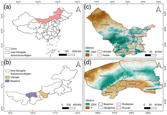
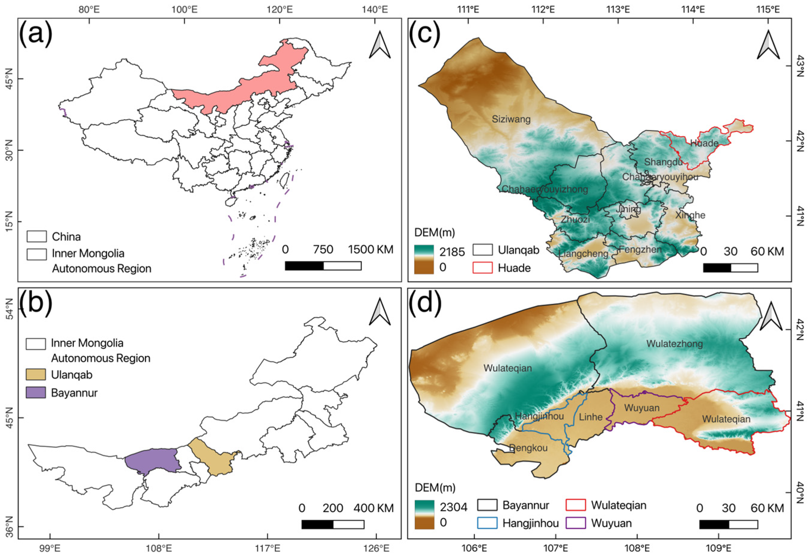
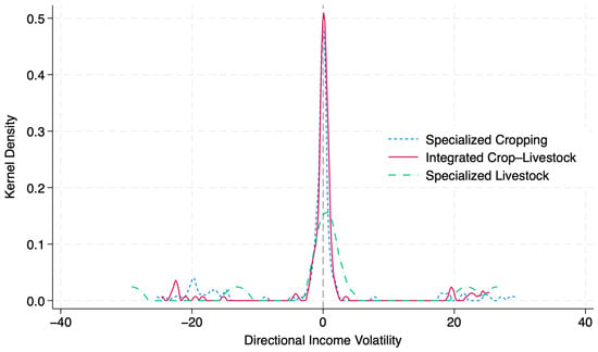
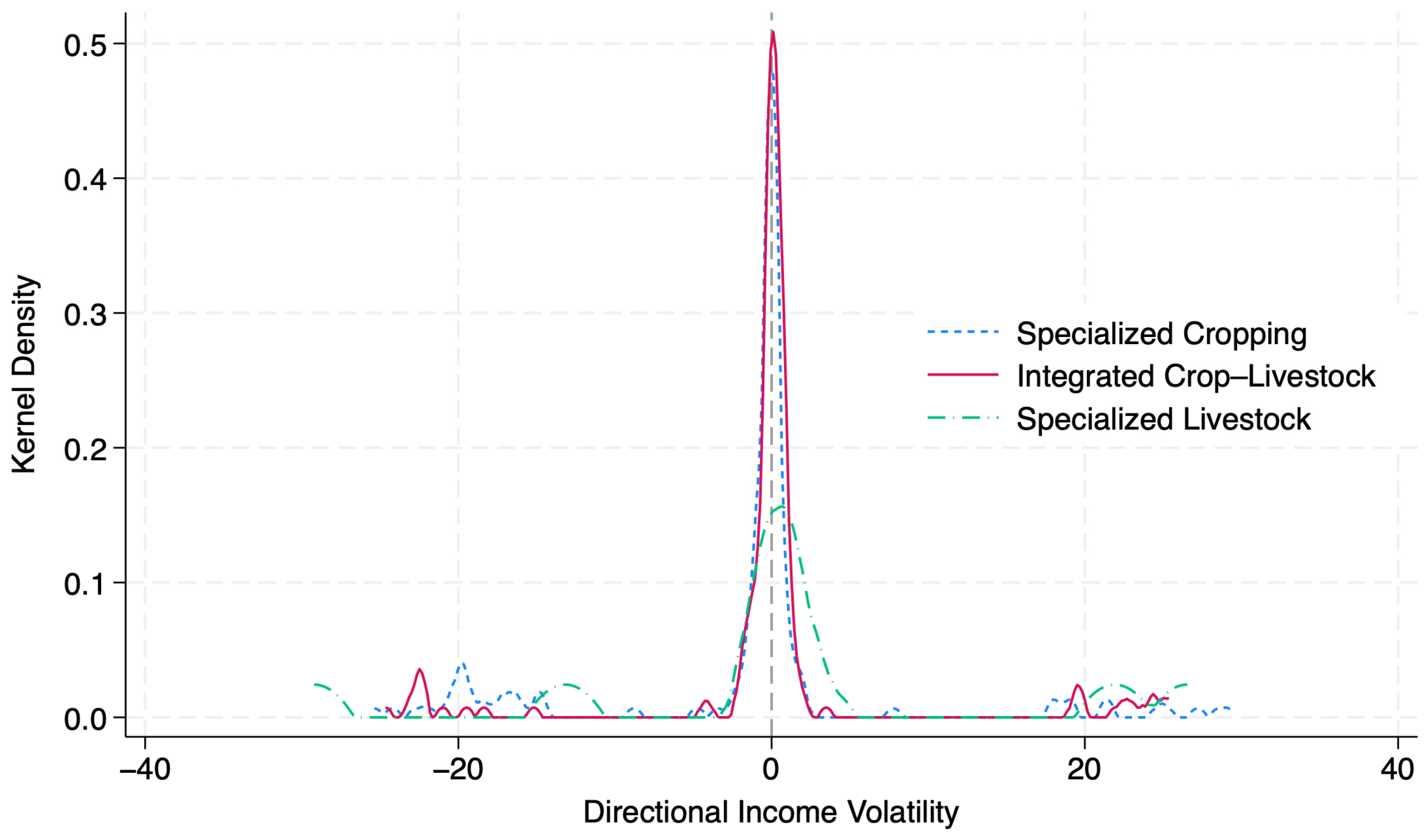

Disclaimer/Publisher’s Note: The statements, opinions and data contained in all publications are solely those of the individual author(s) and contributor(s) and not of MDPI and/or the editor(s). MDPI and/or the editor(s) disclaim responsibility for any injury to people or property resulting from any ideas, methods, instructions or products referred to in the content. |
© 2026 by the authors. Licensee MDPI, Basel, Switzerland. This article is an open access article distributed under the terms and conditions of the Creative Commons Attribution (CC BY) license.